A Strategy for Mouing a Mass from One Point to Another

by BR~~EH.KARNOPP,FRANCI~E.FISHER and BYUNOOK~~~N

Department of Mechanical Erujineering, University of Michigan, Ann Arbor, MI 48109-2125. U.S.A.

ABSTRACT : In many circumstances, it is desired to move a mass from one position to another without initiating a vibration in the mass being moved. Two such problems are considered here : the motion of a mass initiated by another mass, and the motion of a pendulum initiated by the spectfied motion of its support. In each case, it is desired that the system start at rest and come to rest in the second position. A simple strategy for the spect$ed motion is given here. The method is motivated by engine cam-follower design. The force required to move the system in question is determined as well as the maximum value of the force required (and the times at which these forces take place) is determined.

I. Introduction

In several circumstances, it is desired to move a mass from one position to another without inducing any vibration in the mass being moved. Examples include cam-follower systems in engines, recording heads on computer disk drives and the motion of robot arms. In fact, the general design of a typical engine cam gives the motivation for the specified motion we attempt below. There are several approaches to the problem posed here, see, for example (1,2).

II. Moving a Mass from One Point to Another

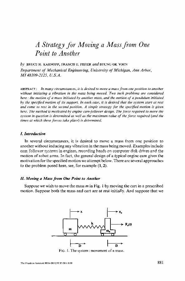
Suppose we wish to move the mass m in Fig. 1 by moving the cart in a prescribed motion. Suppose both the mass and cart are at rest initially. And suppose that we

l-77 l-77 FIG. 1. The system : movement of a mass.

TheFranklin lnstitute00lf4H32/92 $5.oO+O.Ml 881

B. H. Kurnopp et al.

wish to move the cart so that the mass m comes to rest again after a displacement D.

The differential equation of motion of the mass m is

F, = ma, : k[x,(t) - x] = m.2

or

.;t_tC$X = co;.&(t),

where

(1)

(1’)

co,, = Jkjm.

Since we want m to move a distance D with no overshoot, it is important that the cart move a distance D as well. This means the spring which is unstressed initially will be unstressed in the final position as well. Thus each of the two masses will end up with a displacement D.

In order to accomplish this, let us suppose that the specified displacement has the form :

x,(t) = iD[l -cos(cu,/r)t)], 0 < t < (c(Tc/w,~)

= D, t > (WC/o,). (2)

The motivation for the (1 - cos 0) in (2) comes from typical shapes used in engine cam-follower systems (2). A plot of (2) is shown in Fig. 2. Notice that the shape of the curve gives hope that the strategy might work. Notice also that the speed with which we can make the move is determined by c( since n/w, is fixed.

We will see that the values of a which will work are

c( = 3,5,7,. . .

That is, the frequencies of the prescribed motion x,(t) can be

x,(t)

D,&.- -- - _

882

FIG. 2. Prescribed motion .v,,(t).

Moving a Mass without Vibration

u,/3, w,/5, 0447,. . . , o,/(2n+ I), n = 1,2,3,. . .

We construct the solution to (1’) with the specified displacement x,(t) given by

(2) :

z+fo,2x = $Doi[l -cos (On/CI)t]. (3)

The right-hand side of (3) consists of a constant term plus a cosine term. As such, we guess a particular (forced) solution of the form

XP = P+ Q cos (o,/cc)t, (44

where P and Q are constants to be determined so that (3) is satisfied. Inserting (4a) into (3) and cancelling the common term (w,)‘, gives

P=$D,

The homogeneous solution to (3) has the form

xh = Asin(o,t)+Bcos(o,t)

Adding (4a) and (4b), we get

1 +Asin(o,)+Bcos(w,t).

We determine the constants A and B from the initial conditions :

x(0) = i(0) = 0.

These conditions yield

A = 0, B = $D[~/(u’- I)].

Thus, we have the complete solution :

2

l- 2, cos(o,/a)t+ &, cos(u,t) 1

(4b)

There are two conditions which we must now impose on (5). First, we want x(t,) = D, where t,, = (~rc/w,,). And finally, we want the velocity of m to vanish at t, (i.e. _t(t,) = 0). Note that:

(w,/c() t, = n rad and o,, t, = cm rad. (6)

Thus from (5), we get

The terms inside the [ ] must add to 2 if x(tf) = D. This will happen when cos (an) = - 1 if CX- 1 # 0. Thus, this condition requires

Vol. 329. No. 5, pp. 8X1-892. 1992 Printed in Great Britain 883

B. H. Karnopp et al.

a=3,5,7 ,..., (2n+l).

Now we require that .~?(t,) = 0. From (5) and (6), we get

(a)

a(+) = @o, [

&sin (MC) 1 . @I This expression vanishes if CI = 2, 3, 4,

The terms which are common to (a) and (b) are then the odd integer values of CI from 3 on. Thus the solution for the motion of the mass m is

[

7 x = $D 1 - ;-~~icos(~,/~)If &os(~J) 1 , O<t<t,

= D, tt < t, (7)

where

t, = (an/w,) and LX = 3,5,7,. . . , (2n+ 1).

A plot of x,(t) and x(t), the specified motion of the cart and the resulting motion of m, is shown in Fig. 3. Notice that at tr the distance between m and the cart is the same as it was initially. Thus the spring is unstressed. And since the velocity of m

is zero and the prescribed motion of the cart remains at x, = D, the mass m will remain at rest at the point x = D.

Equation (7) gives the design equation for the motion shown in Fig. 3. As noted, a can take the values 3, 5, 7,. . . . Thus the time required to move the mass m a

distance D is

r, = (cUr/o,). (8)

In order to minimize the time tl, we should select a = 3 and select a large value of

D/2 -* s(t)... cart motion I

I

I

I I

884

FIG. 3. The motion x,(t) and the mass motion .x(t).

Journal of the Franklin Institute Pcrgamon Press Ltd

Moving a Mass without Vibration

the spring constant k (to increase the natural frequency w, = Jkim). The solution is not unique since we can take CI = 3,.5,7,. . . and adjust o, accordingly.

The design equations for the strategy are contained in Eqs (2) and (7). One final consideration is the force F,(t) required to move the cart. Writing F, = m,a,, where a, is the second (time) derivative of the motion (2), we obtain

2FJDk = [(m,/ma’) + 1/(a2 - l)] cos (ant/a) - [l/(a’- l)] cos (co,t), (9)

where

The maximum amplitude of 2FJDk depends on CI and the mass ratio m,/m. Suppose we take CI = 3 (the case for the fastest transit from A to B). Then we can determine the positions and heights of the maximum amplitudes as shown in Table I.

TABLE I

Time and values qf the maximum ,force-mass movement, a = 3

R,, = m,lm

0.0 0.1

0.2

0.3 0.4 0.5 0.6 0.7 0.8 0.9 1.0 1.1 1.2 1.3 1.4 1.5 1.6 1.7 1.8 1.9 2.0 2.5 3.0 3.5 4.0 4.5 5.0

Vol. 329, No. 5, ,,p. 8X1-892. 1992 Pnnted in Great Britain

t I * %/an t z * w,/ax Amp.

W,lW

0.304 0.696 0.192 0.302 0.698 0.199 0.299 0.701 0.205 0.297 0.703 0.212 0.294 0.706 0.219 0.292 0.708 0.225 0.289 0.711 0.232 0.287 0.713 0.239 0.284 0.716 0.246 0.282 0.718 0.253 0.280 0.720 0.260 0.277 0.723 0.267 0.275 0.725 0.274 0.272 0.728 0.282 0.270 0.730 0.289 0.268 0.732 0.296 0.265 0.735 0.304 0.263 0.737 0.311 0.261 0.739 0.319 0.258 0.742 0.326 0.256 0.744 0.334 0.244 0.756 0.373 0.232 0.768 0.414 0.220 0.780 0.456 0.208 0.792 0.500 0.196 0.804 0.544 0.183 0.817 0.590

885

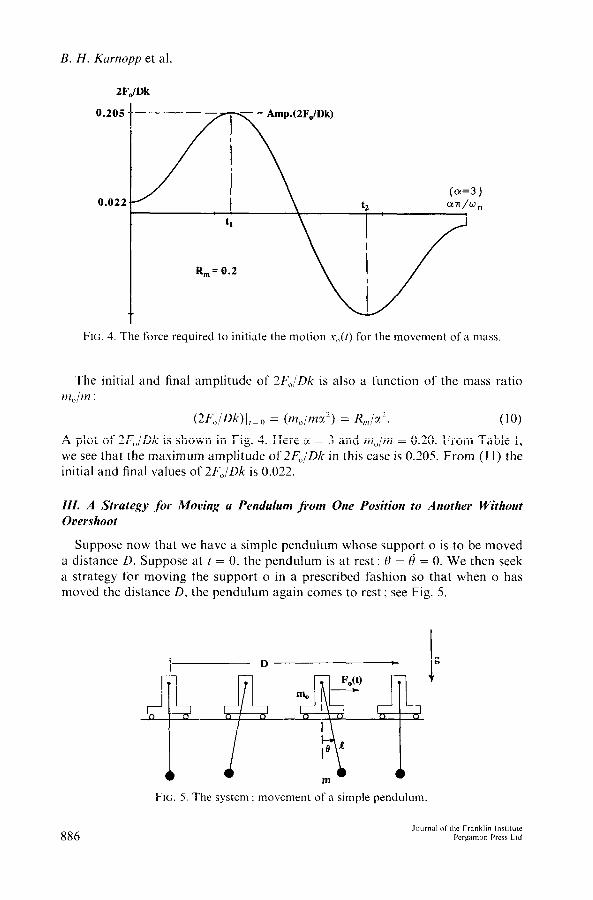
B. H. Karnopp et al

ZF,IDk

0.205

(a=3 ) 0.022

FE. 4. The force required to initiate the motion r,,(t) for the movement of a mass

The initial and final amplitude of 2F,,/Dk is also a function of the mass ratio

m,,/m :

(2F,,/Dk)I,=,, = (m,,/ma’) = R,,,lcc’. (10)

A plot of 2FJDk is shown in Fig. 4. Here x = 3 and m,/m = 0.20. From Table I, we see that the maximum amplitude of 2FJDk in this case is 0.205. From (1 1) the initial and final values of 2FJDk is 0.022.

III. A Strategy for Moving a Pendulum from One Position to Another Without Overshoot

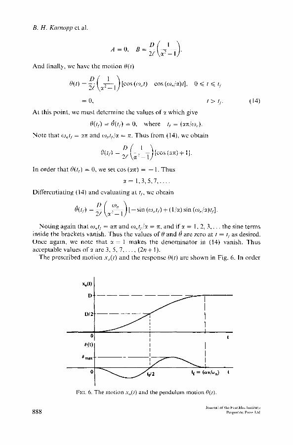
Suppose now that we have a simple pendulum whose support o is to be moved a distance D. Suppose at t = 0, the pendulum is at rest : 0 = 4 = 0. We then seek a strategy for moving the support o in a prescribed fashion so that when o has moved the distance D, the pendulum again comes to rest; see Fig. 5.

FIG. 5. The system : movement of a simple pendulum.

886

Moving a Mass without Vibration

The above situation could be a model for a crane system designed to move material from one point to another. The amount of material moved is unimportant since the design parameter w, = ,&p does not depend upon the mass of the pendulum.

We denote the prescribed motion of o by x,(t). Writing F = ma in the direction perpendicular to the pendulum string. we have

- mg sin 8 mfS’+m.& cos 0.

Suppose the angle 0 remains small so that we can make the approximations

sinO=G and COS~ZZ 1.

Thus we have the differential equation for the pendulum

e+o,:e = -a,//, (11)

where

W” = me.

Suppose that we take the same displacement function as we chose for the problem in Fig. 1 (i.e. Eq. 2):

x,(t) = {D[l -cos (w&t], 0 d t < (a7c/o,)

= D, t > (cut/o,). (2)

From (9), we need the second (time) derivative of x,(t). Thus (11) becomes

@+w,20 = - (Dw,2/2c~~P) cos (o,/a)t, 0 < t < (cur/w,). (12)

The initial conditions are

G(O) = &O) = 0. (12a)

For a particular solution to (12), we try

Q, = Q cos (w,/a)t.

Inserting this in (12) and cancelling the common cosine terms, we get

(1 - l/cr2)Qo,? = -Dw,2/2a2d

or

Q=-; ,2&. ,( > Adding the particular solution to the homogeneous solution, we get

cos (o,/cc)t+A sin (w,t) +Bcos (o,t).

(13)

Imposing the conditions (12a), we determine

Vol. 329, No. 5, pp. X81-892. 1992 Printed in Great Britain 887

B. H. Karnopp et al.

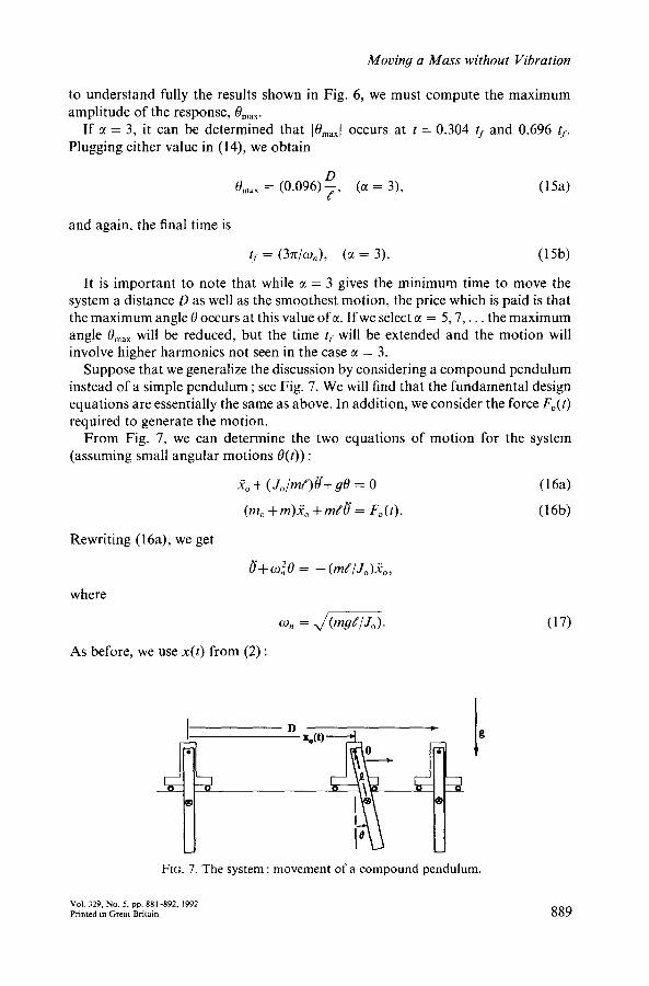
And finally, we have the motion 0(t)

e(t) = ;j A, ( 1 [cos (OJ) -cos (a,,/!+], 0 < t d f,

= 0, t > t,.

At this point, we must determine the values of x which give

tI(t,) = &t,) = 0, where t, = (wx/w,~).

Note that ~,,t, = art and w,,r,/rx = rr. Thus from (14), we obtain

(14)

In order that e(t,) = 0, we set cos (WC) = - 1. Thus

CL= 1,3,5,7 ,....

Differentiating (14) and evaluating at t,, we obtain

f&r,) = p/ & ( > [-sin(o,t,)+(l/cr)sin(w,/x)tll

Noting again that w,t, = cuc and o,,t,/x = rr, and if E = 1, 2, 3,. . the sine terms inside the brackets vanish. Thus the values of 0 and 6 are zero at t = tf as desired. Once again, we note that cx = 1 makes the denominator in (14) vanish. Thus acceptable values of c( are 3, 5, 7,. , (2n+ I).

The prescribed motion x,(t) and the response 0(t) are shown in Fig. 6. In order

FIG. 6. The motion x,(t) and the pendulum motion O(t).

888 Journal or the Frankhn lnst~tutc

Pergamon Prcsr Ltd

Moving a Mass without Vibration

to understand fully the results shown in Fig. 6, we must compute the maximum amplitude of the response, fJmax.

If tl = 3, it can be determined that I@,,,( occurs at t = 0.304 tf and 0.696 tf. Plugging either value in (14), we obtain

Q,,, = (0.096);, (a = 3) UW

and again, the final time is

tf = (37c/oJ, (LX = 3). (15b)

It is important to note that while CI = 3 gives the minimum time to move the system a distance D as well as the smoothest motion, the price which is paid is that the maximum angle 9 occurs at this value of a. If we select tl = 5,7,. . . the maximum angle 8,,, will be reduced, but the time tf will be extended and the motion will involve higher harmonics not seen in the case CI = 3.

Suppose that we generalize the discussion by considering a compound pendulum instead of a simple pendulum ; see Fig. 7. We will find that the fundamental design equations are essentially the same as above. In addition, we consider the force F,,(t) required to generate the motion.

From Fig. 7, we can determine the two equations of motion for the system (assuming small angular motions e(t)) :

R, + (Jojme)8’+ge = 0 (164 (m, +m)R, +md = F,(t). (16b)

Rewriting (16a), we get

8’+o,2e = - (mepo)jt,,

where

0, = J(Gzi.

As before, we use x(t) from (2) :

(17)

FIG. 7. The system : movement of a compound pendulum.

Vol. 329, No. 5, pp. 881-892, 1992 Pnnted ID Great Britain 889

B. H. Kumopp et al.

x,(t) = $D[l -cos (w,/cx)t], 0 < t < (m/o,)

= D, t > (m/w,).

Thus (17a) becomes

ri’+o,;‘e = - (Dw;m//2~‘J,) cos (o,/a)r.

(2)

Comparing this to (12) shows that we can replace (D/2!) in (12) and (13) by (Dm//ZJ,) to get the results for the present case

e(t) = [cos (U&t) -cos (W,,/CL)t], 0 d t G t/

= 0,

Similarly, we can determine Q,,, (here for u = 3) :

o,,,, = 0.096 D;L rad (a = 3) 0

t > t,. (18)

(19a)

and again, the final time is :

t, = (an/to,,), CI = 3,5,7,. . (19b)

To determine the force required to give the motion (IQ, we note the equation (16b):

(m,+m).;t,+m/~= F”(t). (16b)

Inserting -u(t) from (2) and 0(t) from (18), we get

1 (R,,, + 1) + jj@ _1>

I cos (%/~)t?

(20)

where

R,,, = m,/rn and fl = J,lm/ ‘.

Notice that (20) is a function of both the mass ratio R,,, and the moment of inertia ratio /I. In the case of the simple pendulum, J, = nzP’. Thus fl = 1.

In Fig. 8, we plot (20) for the case R,,, = 0.25, a = 3 and fl = 4/3. This is the value of /I for a thin homogeneous bar of length 2rO suspended from one end.

The equation for the force required to move the compound pendulum (21) is a function of the mass ratio R,,, and the inertia ratio fl. The minimum value of fl is 1.0 (for a simple pendulum of length /). Thus R,,, >, 0 and p 3 1. From (20), the initial and final values of (ZF,/Dmo~) are :

Initial and Final (2F,/Dmo,j) = [- l//Y+ 1 + R,,]/cx’. (21)

Clearly if fi > 1 and R,, 3 0, this quantity is greater than or equal to zero. Table II gives the location and maximum values of the required force. Each cell

Mooing a Mass without Vibration

0.056

-0.178

FIG. 8. The required to initiate the motion x,(t) for the movement of a compound pendulum.

TABLE II

Times and value of’ maximum .fovce-pendulum mot’ement, r = 3

&

0.0

0.1

0.2

0.3

0.4

0.5

1.0

2.0

3.0

1 .oo 1.25 1.50 1.75 2.00

0.192t 0.167 0.150 0.139 0.130 0.304, 0.6961 0.298, 0.702 0.292, 0.708 0.286, 0.714 0.280, 0.720

0.199 0.174 0.157 0.146 0.137 0.302, 0.698 0.295, 0.705 0.288, 0.712 0.281,0.719 0.275, 0.725

0.205 0.180 0.164 0.153 0.144 0.299, 0.701 0.292, 0.708 0.284, 0.716 0.277, 0.723 0.270, 0.730

0.212 0.187 0.171 0.160 0.152 0.297, 0.703 0.289, 0.711 0.281, 0.719 0.273, 0.727 0.265, 0.735

0.219 0.194 0.178 0.167 0.159 0.294, 0.706 0.286, 0.714 0.277, 0.723 0.269, 0.73 1 0.261, 0.739

0.225 0.201 0.185 0.175 0.167 0.292, 0.708 0.283, 0.717 0.274, 0.726 0.265, 0.735 0.256, 0.744

0.260 0.237 0.223 0.213 0.207 0.280, 0.720 0.268, 0.732 0.256, 0.744 0.244, 0.756 0.232, 0.768

0.334 0.315 0.304 0.298 0.295 0.256, 0.744 0.238, 0.762 0.220, 0.780 0.202, 0.798 0.183, 0.817

0.414 0.400 0.394 0.392 0.393 0.232, 0.768 0.208, 0.792 0.183, 0.817 0.156, 0.844 0.126, 0.874

t Upper value = Amp. (2FJDmw,f). $ Lower values = t, * w,/m, t, * on/cm.

Vol. 329, No. 5, pp. 881-892, 1992 Printed m Great Britam 891

B. H. Kurnopp et al.

lists the value of the maximum amplitude of (2F,/Dm4 on the top line and the positions of these maxima t , * O,/GYI and t2 * o,/m on the second line.

IV. Conclusions

Simply stated, a mass can be moved from point A to point B without inducing vibration if we use a [l -cos (cot)] specified motion, where w is one third (or one fifth. .) of the natural frequency o, of the system which is being moved. Clearly, the [ 1 -cos (wt)] term must be applied from 0 < t < tl = (c~n/w,,). Taking a = 3 gives the smoothest transition from A to B in the minimum time. In the case of the pendulum, the cost of using (x = 3 is that the amplitude of the pendulum is highest at that value of TY.

A number of questions remain unanswered at this point. For example, we have considered only undamped single degree of freedom systems here. Can the ideas here be expanded to include systems with damping or systems with several degrees of freedom?

If there is damping in a single degree of freedom system, we will not be able to bring 1 to zero at the end of the cycle with the open-loop procedure outlined in this paper. However, the procedure given here could be used in conjunction with a mechanical capture system or a closed-loop control to achieve the desired goal.

Multiple degree of freedom systems can be investigated by using modal analysis, as is done in (4). While this study is outside the scope of the present work, this might prove productive.

References

(I) P. H. Meckl and W. P. Seering, “Minimizing residual vibration for point-to-point motion”, ASME J. Vib. Acoust. Stress Reliubil. Des., Vol. 107, pp. 378-382, 1985.

(2) D. M. Aspinwall, “Acceleration profiles for minimizing residual response”, ASME J. Dyn. Syst. Meas. Control, Vol. 102, pp. 3-6, 1980.

(3) H. A. Rothbart, “Cams-Design, Dynamics, and Accuracy”, p. 238, Wiley, New York, 1956.

(4) J. L. Wiederrich, “Residual vibration criteria applied to multiple degree of freedom cam followers”, ASME J. Med. Des., Vol. 103, pp. 702-705, 1981.

892 Journal of the Franklin lnst,tute

Pergamon Press Ltd