A Structural Model of Entry and Location Choice: The Differentiation–Agglomeration Trade-Off†

Sumon Datta

K. Sudhir

Debabrata Talukdar

August 2007

† Sumon Datta is a doctoral student and K. Sudhir is Professor of Marketing at the Yale School of Management. Debabrata Talukdar is Associate Professor of Marketing at SUNY, Buffalo. The authors thank the participants at the Yale SOM Doctoral Workshop and the 2007 Marketing Science Conference in Singapore for helpful comments on this article.

A Structural Model of Entry and Location Choice: The Differentiation–Agglomeration Trade-Off

Abstract

Extant models of entry and location choices by competing retailers focus on the benefits of differentiation, derived from locating far apart, and therefore cannot explain high degrees of store agglomeration. Unlike extant models that treat firm profits in reduced form, this paper decomposes firm profit as a function of customer choice (to allow for consumer utility from agglomeration) and competition; thus, the authors disentangle the differentiation–agglomeration trade-off that firms face. The findings reveal that (1) consumers value both format and store agglomeration; (2) consumers have high travel costs, and competition among stores decreases dramatically with distance, but ignoring agglomeration benefits biases these estimates substantially; and (3) intraformat competition reduces profitability at roughly twice the rate as interformat competition. Policy simulations demonstrate the importance of modeling the differentiation–agglomeration trade-off to arrive at correct entry and location decisions. Keywords: Retailing, Entry, Grocery, Empirical Industrial Organization

As retailers gain market share, they seek to open new stores to achieve their growth

objectives. For example, Wal-Mart has added approximately 350 new stores each year for the

past five years, and Walgreens expects to increase its stores from 5,580 to 7,000 by 2010.

Perhaps the most famous store expansions are those of Starbucks, which currently operates

12,000 stores worldwide and has a long-term goal of 20,000 stores in the United States and

another 20,000 abroad. On a larger scale, open-air shopping centers, which currently number

around 40,000, are increasing by at least 2% per year on average (Merrill Lynch, 2007). In Table

1, we provide a list of store openings during the period 2001–06, as well as the projected store

openings for 2007, for a cross-section of retail categories.

A growing retailer thus faces two key questions as it embarks on a store expansion

strategy: (1) Should it enter a particular market at all (entry decision), and if so, (2) where should

it locate the new store (location decision)? To arrive at the optimal entry location, the retailer

might analyze detailed consumer-level data regarding how consumers shop across stores in

different markets that vary in terms of population, spending power, and number of stores of

different formats, which vary in their distances from one another. However, this approach is

difficult to implement in practice on a large scale, because such detailed consumer-level data

across markets from multiple retailers are difficult to obtain, and a household-level analysis

across markets can be onerous.

Researchers therefore have adopted an alternative strategy with which they infer the

trade-offs firms face by endogenously modeling entry and location decisions (e.g., Bresnahan

and Reiss 1991; Mazzeo 2002; Seim 2006; Zhu and Singh 2007).1 These models assume that

firm entry and location decisions are an equilibrium outcome, such that firms make their

1 Related literature models consumer choice of spatial locations but treats outlet locations as exogenous (Duan and Mela 2007; Thomadsen 2007). Chan, Padmanabhan, and Seetharaman (2006) also model consumer choice of gasoline outlets when a social planner determines the locations of those outlets.

2

decisions on the basis of the profitability of their choices while accounting for conjectures about

competitors’ decisions. With this approach, decision makers can use readily available data about

entry and location decisions and the demographic characteristics of markets at the reasonably

disaggregate census block level and thus make the necessary empirical inferences.

These studies implicitly assume that spatial differentiation always benefits firms, because

it helps reduce competitive intensity and increase profits. Accordingly, when two firms locate

close to each other in a market, they must do so either because the potential in the market is

extremely large, which enables both firms to be profitable, or because the transportation costs of

customers in the market are high enough that customers are unlikely to price search across firms.

However, this implicit assumption may not be consistent with the data. To explore this

issue, we compare locations in which supermarkets exist less than 0.5 miles apart and locations

in which they are more than 2 miles apart. According to the average characteristics of the

locations in Table 2, the average populations and incomes (total and per capita) actually are not

higher in areas where stores are closer together; rather, they tend to be somewhat lower than

those of areas where firms locate farther apart. Thus, it appears extant models may be missing

features that allow for positive benefits to firms that locate close together.

Why might firms choose to agglomerate? A commonly cited reason is that doing so takes

advantage of customers’ need for “economies of scope” during multipurpose shopping trips (e.g.,

Arentze, Oppewal, and Timmermans 2005). That is, different types of firms may colocate to

facilitate customers’ ability to shop for different types of products at different stores within a

single trip. If consumers value such economies of scope, they should find it more attractive to

shop in locations with greater business density. In this sense, extant research considers the

3

potential benefits of agglomeration around other retail business (exogenous to the model) (e.g.,

Seim 2006; Zhu and Singh 2007).

But do consumers value agglomeration of stores within the same category selling similar

products (e.g., grocery stores)—and should we expect an endogenous agglomeration of stores

belonging to the same category? Because different grocery formats (e.g., supermarkets,

superstores) may provide different types of products at different prices, scope economies of

shopping may make it more attractive for customers to shop in locations that host stores of

different formats. Consumers thus may value “format agglomeration.” Even within stores of

similar formats, consumers may prefer some subset of products at one store. For example, a

shopper may prefer the bread at one store and the vegetables and meat at another store with a

similar format. In this case, the consumer also values “store agglomeration” within the format.

Bester (1998) and Fischer and Harrington (1996) provide such arguments based on the product

heterogeneity across stores.

Finally, another benefit of colocation for consumers involves resolving the hold-up

problem (Wernerfelt, 1994), which can lead to higher prices. When a competitor is close by, a

store is unlikely to raise its prices too much for fear that customers will simply switch to the

competitor. However, when the competitor is farther away, stores have an incentive to “hold-up”

consumers and charge a higher price, because customers in the store will find it costly to visit a

competitor relative to purchasing at the store. A customer fearing higher prices due to hold-up

likely frequents locations with multiple colocated stores, so store or format agglomeration may

represent a means to avoid the hold-up problem.2 Generally, we expect greater benefits of hold-

2 The arguments underlying Wernerfelt (1994) were also made by Stahl (1982), who notes that consumers value the reduction in search costs due to store co-location and Dudley (1990) who notes that customers’ expectations of lower prices in clustered stores can serve as an incentive for stores to colocate.

4

up avoidance associated with store agglomeration than with format agglomeration, because

stores of the same format are closer substitutes than stores of different formats.

To model these theories, we follow Seim (2006) and assume idiosyncratic differences in

profitability among firms, which competitors know only in distribution. The asymmetric

information specification offers the practical advantage of allowing the model to accommodate a

large dimensional set of product types (in our case, locations and formats) because it simplifies

the computation of equilibrium strategies.

The key modeling issue thus becomes how to disentangle the differentiation–

agglomeration trade-off. We decompose the reduced form profit model into separate components

that account for consumer and competitive effects and thus offer an innovative approach to this

problem. By explicitly modeling how transportation costs due to the distance between stores and

the agglomeration of different stores and formats affect consumer utility (and thus location

choice), we clarify the differentiation–agglomeration trade-off. Furthermore, we aggregate the

probabilities that consumers will shop at a particular location, on the basis of the utility model,

by appropriately weighing both the number of these consumers and their spending potential, as

represented by their per capita income, to arrive at the total profit potential of that location.

On the supply side, unlike existing entry literature that assumes firms are symmetric (cf.

Zhu and Singh 2007), we allow for the observable profitability of firms to differ according to

format (i.e., cost or efficiency differences). Thus, entry and location decisions are functions of

the format of the store. For example, a Wal-Mart supercenter may have a cost advantage over

other grocery formats. Furthermore, we model the effects of competition in a flexible,

semiparametric manner by allowing profit potential to split differentially across firms as a

function of the format and distance. Thus, two stores of the same format within a one-mile radius

5

may compete much more than do two stores of the same format that are two miles apart.

Similarly, two stores of different formats may compete less than do two stores of the same

format at the same distance. For example, consider the grocery market in Southern Connecticut,

in which two major supermarkets, Stop and Shop and Shaw’s, compete against Wal-Mart

supercenters and a variety of smaller stores. Using symmetric models, Stop and Shop would

simply consider the number of competitors in the market; in our model, the extent of competition

depends on which competitor. For example, when controlling for distance, Stop and Shop could

engage in greater competition with Shaw’s because of its similar format than it does with Wal-

Mart.

When estimating multi-agent, discrete, strategic games, an important challenge relates to

the possibility of multiple equilibria. Specifically, with an incomplete information set-up, for a

given vector of model parameters θ, if there exists more than one set of equilibrium probabilities

of firms’ actions, the likelihood function cannot be well defined. In general, the probabilistic

nature of firms’ conjectures in the incomplete information set-up makes uniqueness easier to

attain than it would be in a complete information set-up, because the necessary conditions for

uniqueness are weaker in the former (Aradillas-Lopez 2005). To deal with this problem, one

approach provides sufficient conditions for uniqueness of equilibria that the model parameters θ

must satisfy. For example, Siem (2006) and Zhu and Singh (2007) discuss sufficient conditions

for uniqueness for special cases of payoff functions they use in their estimations. In this article,

we check ex-post whether conditions for the uniqueness of equilibrium are satisfied at the

estimated parameter values. Alternatively, we could circumvent the requirement that there be

unique equilibria, as do Ciliberto and Tamer (2006) and Bajari and colleagues (2006), as well as

Ellickson and Misra (2007), who extend Bajari and colleagues’ approach in their study of choice

6

of pricing format (e.g., everyday low price versus high–low pricing). Recently, Su and Judd

(2007) have developed mathematical programming with equilibrium constraints approaches that

are both efficient and avoid the multiple equilibria problem.

Although several stores in our data set are chain stores, we assume that entry and location

choices in different markets are independent. This assumption appears in all extant literature,

except Jia (2007), who allows for interdependencies across markets for chain stores. Jia (2007)

also allows for the scale economies that Wal-Mart enjoys by operating multiple stores in nearby

regions. However, with the data we were able to obtain, this issue is beyond the scope of this

article.

Our subsequent analysis leads to several interesting insights. First, consumers value both

format and store agglomeration. Second, consumers experience high travel costs, and

competition between stores decreases dramatically as the distance between them increases.

However, if we ignore the agglomeration benefits, as does extant research, the estimates of travel

cost and the relationship between competition and distance are substantially downward biased.

Third, as we expected, intraformat competition reduces profitability roughly twice as much as

does interformat competition; that is, similar store formats compete more intensely than do

differentiated formats. Fourth and finally, we use counterfactual simulations to show that failing

to account for the differentiation–agglomeration trade-off in consumer utility can lead to

erroneous entry and location decisions. That is, biases in estimates adversely affect managerial

decision making.

The rest of this article is organized as follows: In the next section, we present the model

for joint entry, format and location choices of firms and describe the estimation approach. After

7

we describe the data, we detail the results and their implications. We conclude with a discussion

and some directions for further research.

Model Set-Up

We develop a model of simultaneous entry and location choices that can disentangle the

agglomeration–differentiation trade-off. Most research in entry and location literature models

profit potential at a location as a reduced form that subsumes consumer and competitive effects.

However, because we want to distinguish agglomeration benefits that arise from consumer

shopping behavior and the differentiation benefits that result from competition moderation, we

decompose the profit potential into consumer and competition components.

Consumers’ Location Choice

Each geographic market m (m = 1, …, M) consists of a set of smaller locations (l = 1, …,

Lm). Consumers in these locations may shop at any of the grocery stores in the market. Let 0α be

the base utility a consumer obtains from shopping at a grocery store and 1α be the travel cost per

unit of distance. Thus, the intrinsic utility of shopping at a grocery store at location l for a

customer at location i equals ild10 αα − , where dil is the distance the customer must travel.

If economies of scope result from multipurpose shopping areas, a location becomes more

favorable if it has a greater business density in connection with retail stores that cater to the

consumers’ nongrocery needs (e.g., electronics, clothing). To capture such scope economies of

shopping, we consider the number of retail stores in location l; to capture scope economies of

shopping within the grocery sector specifically, we also integrate the effect of the presence of

grocery stores of different formats in that location (i.e., format agglomeration effect) on

consumers’ utility. Furthermore, because a customer who fears hold-up likely frequents locations

8

where stores colocate, we include the number of other grocery stores within 1 mile of location l

(i.e., store agglomeration effect).

Formally, for a consumer in location i, the utility of shopping at location l is specified as:

ilMFlllilil INretdU ωααααα ++++−= 43210 , (1)

where

α0 base utility of shopping at a grocery store;

dil linear distance between locations i and l;

α1 dil disutility of traveling to location l;

retl number of retail businesses in location l;

2α retl utility of shopping at a location l with retl businesses;

Nl number of grocery stores within 1 mile of location l;

α3 Nl store agglomeration utility of shopping in a cluster at location l;

IlMF indicator of the presence of multiple formats within 1 mile of location l;

α4 IlMF format agglomeration utility from shopping at a location with multiple formats;

and

ilω unobserved characteristics of locations (e.g., traffic patterns, longer travel times

due to geographic characteristics)

We cannot infer the actual value of ilU but can determine the difference in utilities of

two options. Specifically, for the consumer at location i, we consider the difference in the utility

associated with shopping at location l and the utility derived from shopping at location i,

il iiU U− . Assuming i.i.d. Type 1 extreme value distribution for the unobserved errors, the

probability that a consumer at location i will visit location l is

9

1 2 3 4

1 2 3 4

exp( ( ) ( ) ( )1 exp( ( ) ( ) ( ))

MF MFc il l i l i l iil MF MF

ij j i j i j ij i

d ret ret N N I Ipd ret ret N N I I

α α α αα α α α

≠

+ − + − + −=

+ + − + − + −∑. (2)

This equation indicates the share of consumers living in location i who will shop at location l.

Linking Consumer Location Choice to Location Profit Potential

To arrive at the profit potential of location l, we aggregate the contribution of consumers

of each location who will shop at location l. We first specify the total income that consumers

from location i have available for spending in location l, ( ilInc ). In particular, we weigh the

location choice probabilities of consumers, derived from the utility model, by the number of such

consumers and their spending potential, as represented by their per capita income:

cil il i iInc p Pop PCI= , (3)

where

Popi population of location i;

cil ip Pop number of consumers of location i who visit location l; and

PCIi per capita income of consumers at location i.

To obtain the total income available for spending in location l, we sum the contributions from all

locations in the market:

1

mL

l ili

Inc Inc=

=∑ . (4)

If we denote the market characteristics of retail businesses, population, and per capita

income by Xm, the profit potential of location l, which we denote as ( , , ; )m m MFl lf X N I α , then can

be specified as

5( , , ; )m m MFl l lf X N I Inc αα = . (5)

10

Competitive Effect

If a firm f with format k (k = 1, …, K) chooses to enter location l, it must share the profit

potential at location l with its rivals in the market because of the competitive effect. We model

this effect in a flexible, semi-parametric manner so that we can split the profit potential

differentially across firms as a function of their format and distance. For distance, we follow

Seim (2006) and model competition in terms of discrete circular distance bands (b = 1, …, B)

from the location l. However, unlike existing entry literature, we allow for asymmetric

competitive effects between store formats, such that the intraformat competitive effect may be

different than the interformat competitive effect. Thus, two stores of different formats may

compete less with each other than would two stores of the same format. Furthermore, the

intraformat competitive effect may differ for different formats.

Let bmtlN denote the number of rivals of format or type t (t = 1, …, K) in distance band b

around location l within market m. If we denote the competitive effect as

'( ,..., ,..., ; )m m mk k Kh N N N β , where m

tN is the number of rivals of format t in the market, the

competitive effect for firm f can be specified as:

'' '

'

( ,..., ,..., ; ) (1 ) (1 )kb k bm m m bm bmk k K kl k l

b b k k

h N N N N Nβ ββ≠

= + +∏ ∏∏ . (6)

The first component on the right-hand side of Equation 6 is the intraformat competitive

effect; the second component is the interformat competitive effect. We use this multiplicative

specification to demonstrate that the competitive effect of an additional rival should decrease

with the number of rivals. Adding 1 to the number of rivals captures the idea that in the absence

of rivals within a particular distance band b, there is no competitive effect for firm f in that

distance band.

Firm Profits

11

Firms make entry and location decisions on the basis of the profitability of their choices,

consumers’ shopping behavior, and their conjectures about competitors’ entry and location

decisions. They also choose whether to colocate with a rival of the same format or a different

format depending on the resulting total profit potential, f(.), of a location and the effect of

competition, h(.), on profits. Whereas the benefits of agglomeration occur through increased

profit potential, the benefits of differentiation emerge from acquiring a greater share of that

potential as a result of decreased competition.

Formally, a firm f from an exogenous potential pool of F entrants (f = 1, …, F) decides

whether to enter market m with format k, and if it decides to enter, it decides whether to choose

location l. Upon entry into location l, firm f’s profit is

'( , , ; ) ( ,..., ,..., ; )m m m MF m m m mfkl l l k k K k flf X N I h N N Nα β τ η ξΠ = , (7)

where τk is a format-specific scaling factor, flη is an idiosyncratic firm- and location-specific

scaling factor, and mξ is a market-specific scaling factor. We assume that flη is idiosyncratic and

known only to the firm, and rivals know it only in distribution. Therefore, we introduce

information asymmetry into the model, which we exploit for computing the equilibrium. The

market-specific scaling factor mξ controls for the unobserved attractiveness of the entire market

and thus partly determines the number of firms a market can support. Unlike existing entry

literature, which assumes that firms are symmetric (cf. Zhu and Singh 2007), we allow for

asymmetric competitive effects. Further, we allow the intrinsic profitability of firms to differ in

their format (i.e., due to either cost or efficiency differences) according to a format-specific

parameter τk. We normalize this parameter to 1 for one of the formats for identification.

The proposed model nests simpler models with no agglomeration effects or those with

homogeneous stores. Without agglomeration effects, the profit potential of a location is driven

12

completely by exogenous characteristics mX , as has been assumed in previous literature. Thus,

the effect of the number of neighboring stores mlN and the presence of multiple formats MF

lI

would not be needed in the potential function f(.). The resulting specification for mfklΠ would be

'( ; ) ( ,..., ,..., ; )m m m m m mfkl k k K k flf X h N N Nα β τ η ξΠ = . (8)

If stores cannot be distinguished by formats, all stores are homogenous, and the

competitive effect h(.) is due only to the total number of rivals that enter the market Nm, and the

format-specific scaling factor (τk) is not needed. The resulting specification for mfklΠ would be

( ; ) ( ; )m m m mfkl flf X h Nα β η ξΠ = . (9)

Thus, the simpler models are embedded in our model.

Equilibrium Choice Probabilities of Firms

Because we consider a joint entry and location choice model, when the decision makers

make that choice, the profitability of a store operating in a location is a function of the expected

number of rivals of various formats that might enter the market and choose a certain location. A

firm cannot observe its rival’s idiosyncratic component of profitability but can recognize its

distribution, so it can form a conjecture or assign a probability to a rival’s choice of a location.

The expected competitive effect of different rivals in different distance bands is given by:

''

'

(.) (1 [ ]) (1 [ ])kb k bbm bmkl k l

b b k k

h E N E Nβ β

≠

= + +∏ ∏∏ , (10)

where

[ ] *bm

bm m mkl kj

j L

E N N p∈

= ∑ (11)

13

is the expected number of rivals of format k that choose a location in distance band b when Nm

rivals enter the market, and mkjp is the probability of a choice of location j (which lies in distance

band b) in market m by a firm of format k.

Similarly, on the basis of its conjectures about rivals’ and its own actions, the firm

calculates an expected potential of the location using expected consumer behavior. Hence,

Equation 1 transforms into:

ilMFlllilil IENEretdU ωααααα ++++−= ][][ 43210 . (12)

In equilibrium, when a firm makes its optimal choices, the resulting strategy, in terms of

choice probabilities, matches the strategy of rivals of the same type in each format. Therefore, in

equilibrium, the conjectures of each firm about the strategies of all rival firms matches those

rival firms’ actual equilibrium strategies. This matching demands a nested fixed-point problem in

the form of a mapping of the firm’s strategy (which is a function of the competitors’ strategies)

onto competitors’ strategies (which is a function of the firm’s strategy).

To illustrate the fixed point problem, we take the log transformation of the firms’ profit

function (Equation 7):

5 ' ''

ln( ) ln( ) ln(1 ) ln(1 ) ln( ) ln( ) ln( )m bm bm mfkl l kb kl k b k l k fl

b b k kInc N Nα β β τ η ξ

≠

Π = + + + + + + +∑ ∑∑ .

(13a)

For ease of exposition, we denote the left-hand side as mfklΠ~ and group the potential and

competitive effects together, denoted as mklΠ

~, such that

5 ' ''

ln( ) ln(1 ) ln(1 ) ln( )m bm bmkl l kb kl k b k l k

b b k kInc N Nα β β τ

≠

Π = + + + + +∑ ∑∑ . (13b)

14

Also, by denoting the idiosyncratic component as flυ and the market-specific component as mξ ,

we can rewrite Equation 13a as

mfl

mkl

mfkl ξυ ++Π=Π

~~ . (13c)

We assume that the idiosyncratic component follows a Type 1 extreme value distribution

and is independent across firm-location combinations.3 Moreover, we normalize the profitability

of not entering the market to 1 (i.e., log transformation equals 0).4 Let the vector of the

equilibrium location choice probabilities [ mkL

mk

mk mppp ,...,, 21 ]’ of rivals of type k (k’) be denoted by

*mkP ( *

'm

kP ). Because the market-level unobserved effect mξ is common to all locations, it does

not influence the choice of locations after the firm has decided to enter the market. The

probability of the choice of a location l by a firm entering as type k thus is given by the logit

form:

KkLlp m

mkg

L

g

K

k

mklm

kl m ,...,1,,...,1)

~exp(

)~

exp(

11

=∀=∀

⎟⎟⎟⎟⎟

⎠

⎞

⎜⎜⎜⎜⎜

⎝

⎛

Π

Π=

∑∑==

. (14)

This system of (K*Lm) equations define the equilibrium location choice probabilities as a

fixed point problem. The probabilities of choosing a format and location, conditional on entry,

must add up to , we essentially have a system of K*Lm 1 equations in K*Lm 1 unknowns. firm’s

strategies are continuous in its rivals’ strategies, by Brouwer’s fixed point theorem, at least one

solution exists for this system of equations. Note that since the market-level unobserved

3 This assumption does not allow for correlations in profitability across firms for the same location or across locations for the same firm. Such considerations are beyond the scope of this research. 4 This normalization may be rationalized as a fixed-entry cost that is symmetric across all firms.

15

effect, mξ , is common for all locations, it does not influence the choice of locations once the firm

has decided to enter the market.

The total number of firms from the pool of F potential entrants that enter the market is

determined by the attractiveness of the locations in the market for all firms and the unobserved

market-level term mξ . Because the profitability of not entering the market is normalized to 1

(log transformation equals 0), the probability that a firm enters the market is given by:

Pr(Entry) =

⎟⎟⎟⎟⎟

⎠

⎞

⎜⎜⎜⎜⎜

⎝

⎛

Π+

Π

∑∑

∑∑

==

==

)~

exp(*)exp(1

)~

exp(*)exp(

11

11

mkl

L

l

K

k

m

mkl

L

l

K

k

m

m

m

ξ

ξ. (15)

Hence, the total expected number of entrants in the market, (Nm + 1), is given by:

( mN +1) = F * Pr(Entry). (16)

By fixing the potential number of entrants F and observing the actual number of entrants (Nm+1),

mξ can be estimated as

1 1

ln( 1) ln( 1) ln( exp( ))mK L

m m m mkl

k lN F Nξ

= =

= + − − − − Π∑∑ . (17)

We assume that mξ follows a normal distribution, ),( σμN , whose parameters can be

estimated on the basis of the vector of mξ across the set of markets. Although the pool of

potential entrants F is not observed, varying the size of this pool should have only a miniscule

effect on the location choices, because mξ adjusts accordingly, relative to the outside option’s

fixed effect (i.e., choosing not to enter). Hence, we fix the pool size exogenously as twice the

actual number of observed entrants. Alternatively, F could be fixed as a large number for all

markets (e.g., F = 30).

16

Because the probability of entry is a function of the firms’ equilibrium conjectures, which

in turn is a function of the number of firms that enter the market, a simultaneous solution for this

set of equations provides the joint equilibrium predictions for the location choice probabilities

and the number of entrants.

Estimation

We identify three store formats in the markets that we analyze and thus tailor our model

to three formats (K = 3). If we drop the band subscript and denote the competitive effect between

format k and format k’ as βkk’, intraformat competition is given by βkk. We estimate the model by

maximum likelihood with a nested fixed-point function to estimate the equilibrium location

choice probability vectors, * *1 2,m mP P , and *

3mP , of the firms in each market.

Starting with an initial guess for the parameter vector θ (= [α, τ, β, μ , σ]), we first set the

probability vectors to 0 in each market. For every market, we can predict consumers’ shopping

behavior to find the expected potential of each location in the market; then we calculate the

elements of the probability vectors as given by Equation 14. We repeat this process for each

market until we reach the fixed-points, * *1 2( ), ( )m mP Pθ θ , and *

3 ( )mP θ . Finally, we estimate mξ as

in Equation 17.

The equilibrium probabilities of the observed location choices, stacked across firm types

and markets, enters the conditional likelihood function:

L( σμθ ,1 ) = ∏∏∏=

=ΙM

m k

llmmmlk

l

mkNXp

1

)(1 )),,(( θ , (18)

where θ1 =[α, τ, β]), and I(l = lkm) = 1 if location l is chosen by a firm of type k and is 0

otherwise. The unconditional likelihood function is:

L(θ) = ),,(*(.))(1

)( σμξφ mM

m k

llmlk

l

mkp∏∏∏

=

=Ι , (19)

17

where φ (.) is the pdf of the normal density.

As we discussed previously, a challenge of this estimation approach is the possibility of

multiple equilibria. The system of equations for the conditional location choice probabilities is:

(p, X, N) p - F(p, X, N) = 0Ψ = . (20)

A solution is ensured by Brouwer’s fixed-point theorem. The sufficient condition for uniqueness

is that the matrix of partial derivatives of Ψ with respect to p is a positive dominant diagonal

matrix, or that

(21)

We verify ex post that the unique equilibrium criteria are satisfied at the estimated parameter

values.

Identification

To identify our model with agglomeration–differentiation effects, (1) the model must

make different predictions for where firms will agglomerate or differentiate as a function of the

market characteristics and (2) there should be sufficient variation in the market characteristics

that would predict agglomeration in some markets and differentiation in others. According to the

model, when concentrations of consumers with high incomes that can sustain stores on their own

exist, firms choose to differentiate and avoid competitive effects. But when the concentration of

local market potential cannot support a store and consumers and incomes are more dispersed,

firms choose to agglomerate through colocation. Colocation also should be greater when

business density is disproportionately high in certain areas, which increases that location’s

market potential because of its ability to attract new customers from outside the location.

We determine whether the data are consistent with this identification argument and report

the coefficients of variation (standard deviation/mean) for population, income, and business

density in Table 3. Agglomeration is greater in areas where populations and income are more

0l

l

l l

k ll k

p

p p≠

∂Ψ>

∂

∂Ψ ∂Ψ≥

∂ ∂∑

18

spread out, that is, where the coefficient of variation is greater. Agglomeration also is greater in

locations with higher business density (see Table 2) and a lower coefficient of variation in

business density. The coefficient of variation varies considerably across locations (in most cases,

the standard deviations are comparable to the means). Thus the two characteristics above are

satisfied, which enables us to identify the model.

Data

Description of Data

For our analysis, we use a data set obtained from a traditional supermarket chain, which

we henceforth call Chain A. The chain operates in several states in the United States, and we

possess data from 146 markets in which this chain’s stores are located. We use the same

definition for a market as that used by Chain A, based on a trade radius that it considers

appropriate, given the competitive structure of grocery markets. The trade radius is smaller for

urban markets and larger for rural markets (average = 4.44 miles for urban markets and 7.16

miles for rural markets). We also gather data on the coordinates (latitude and longitude) of all

major grocery stores in these 146 markets. Each market consists of several hundred census

blocks, for which we have data about the coordinates and demographics. To simplify our

analysis, we define a location as a collection of some number of census blocks, identified by 12-

digit codes: SS-CCC-BBBBBBB. The first two digits represent the state, the next three represent

the county, and the last seven digits stand for the specific census block. We group census blocks

with the same first nine digits to define a location.5 This approach divides each market into a

reasonable number of locations. We assume the coordinates of each location are the averages of

5 Some applications (Seim 2006; Watson 2007; Zhu and Singh 2007) that work with census tracts group several tracts (e.g., those within a county with the same first three digits) to define a location.

19

the coordinates of the census blocks within that location; consistent with existing literature, we

assume all consumers and stores within a location appear at these coordinates.

We supplement the demographic data with data pertaining to the number of retail

establishments at the zip code level, obtained from the U.S. census. Therefore, we assume that a

location belongs to the zip code that is nearest to it (the U.S. census also provides coordinates of

the zip codes) and that the retail establishments are distributed uniformly across the locations

within a zip code. We take this approach because retail establishment data are available only at

the zip code level, not at the census block level, and we do not expect any systematic errors as a

result. In Table 4, we present the summary statistics for our data.

Identification of Store Formats

Data on store interaction ratings identify the different formats of grocery stores operating

in these markets. Chain A rates its competitors in each market according to the extent of their

interaction. These interaction ratings are based on the similarity in store formats and the overlap

between their trade areas. In Table 5, column A, we provide the mean interaction ratings of

different store chains across all markets. Over all markets, we ran regressions of interaction

ratings across different store chains and their distances from the focal Chain A store. In Table 5,

Column B, we provide estimates of the individual regressions and interaction ratings for each

store chain after we control for distance.

On the basis of the estimates in Table 5, we cluster store chains B and C as closest to

Chain A in terms of store format, followed by store chains D and E, and then the remainder. Our

knowledge of the grocery market indicates that store chains A, B, and C actually employ a

supermarket format (SMF),6 whereas chain D follows a superstore format (SSF), and store chain

6 Articles from the popular press suggest that in the markets we analyze, these three store chains were very close competitors for the period that we analyze.

20

E is similar to a SSF. We group the other store chains, which include food stores, dollar stores,

limited assortment grocery stores, warehouse clubs, and others, into a third type, which we call

the “Other” store format (OSF).

Results

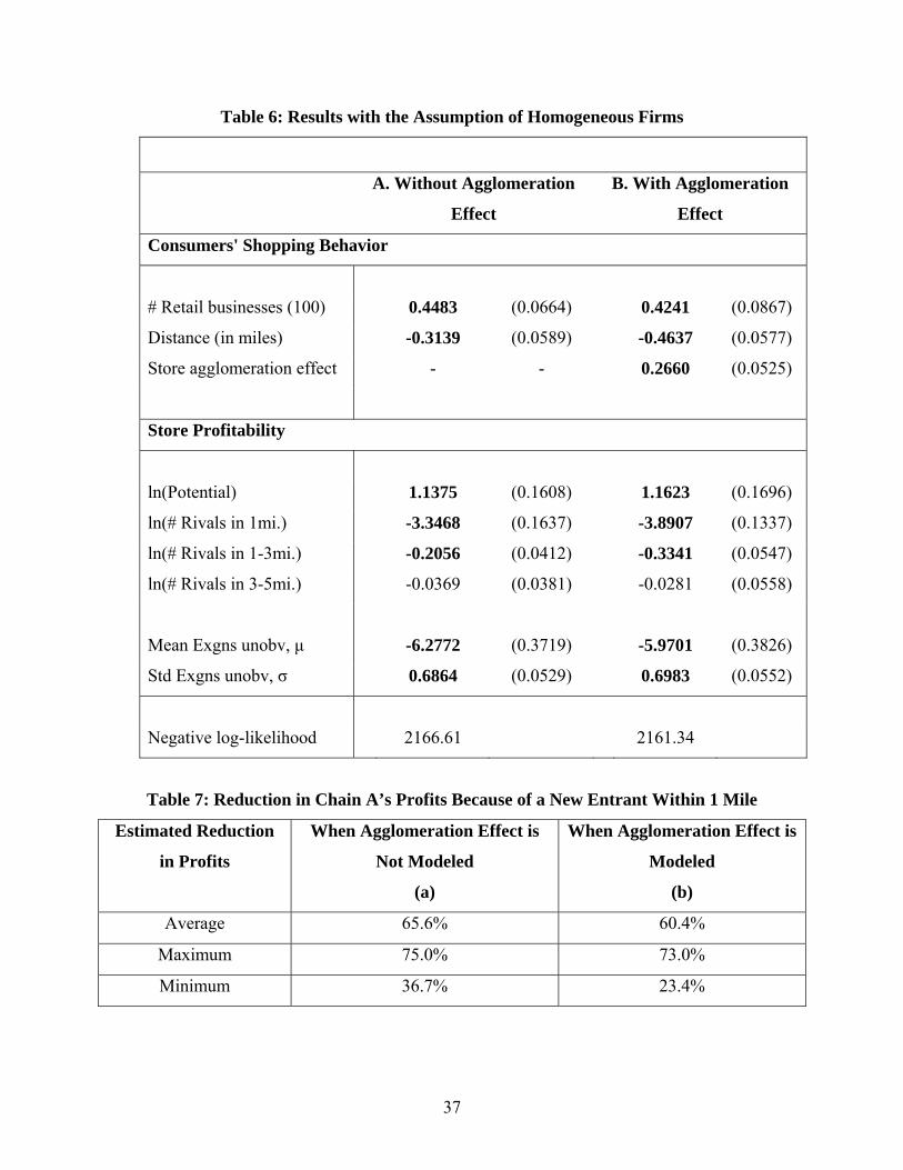
Homogeneous Firms

We present the results for a benchmark model with only homogeneous firms in Table 6.

Here we compare estimates with and without modeling the agglomeration effect. Because of the

homogeneity assumption in this benchmark model, we account only for the store agglomeration

effect, not the format agglomeration effect.

We consider three distance bands of less than 1 mile (b0), 1–3 miles (b1), and 3–5 miles

(b2). The log-likelihoods demonstrate that accounting for agglomeration effects significantly

improves the fit (p < .001). Both model estimates have the expected signs. Consumers

experience disutility from traveling to stores; they value a location with more retail businesses (#

Retail Business), consistent with the economies of scope hypothesis. The coefficient for potential

is not significantly different from 1, which suggests that stores choose locations under the

premise that grocery spending for consumers is proportional to their income. In both cases,

competitive effects decrease dramatically with distance. Rivals that are more than 3 miles away

have negligible impacts on each other, which is not surprising in grocery markets, because

consumers tend to shop at nearby supermarkets7. In our subsequent analysis, in which we

distinguish formats, we consider only the first two distance bands to reduce the estimation costs.

We find clear evidence for a store agglomeration effect. Not only does the model with

store agglomeration effects fit the data better but ignoring it biases estimates of both consumer

7 As per the International Council of Shopping Centers’ classification of shopping centers (DeLisle, 2005), a Neighborhood Center with a supermarket as its anchor store has a primary trade radius of 3 miles.

21

utility and competitive effects. The estimates that fail to model store agglomeration

underestimate both the consumer’s disutility from travel for shopping and the competitive effect.

This is expected because in the data when consumers and incomes are more dispersed and stores

collocate, the simpler models incorrectly predict that consumers must be willing to travel greater

distances (i.e., they have a lower disutility from travel), and that the competitive effect must be

low, which allows stores to collocate. Specifically, the model without store agglomeration

estimates disutility per mile for shopping as –.3139, whereas the corresponding estimate for the

model with store agglomeration is –.4637, a 47% difference. Similarly, failing to account for the

store agglomeration effect underestimates the competitive effect.

To understand how the competitive effect affects profits, we compute how profits of

Chain A stores change with the addition of a new competitor in the different distance bands.

New entry affects both customer choice and competitive effects. If a competitor agglomerates

with an existing store at a distance of 0–1 miles, the change in profits results from the increased

potential of the location because of the agglomeration and also from the increased competition

because of colocation.

If the store agglomeration effect is not modeled (Table 7, column a), when a new

competitor decides to enter within 1 mile of Chain A stores in all markets, the store’s profits are

estimated to decrease by an average of 65.6% (maximum = 75%; minimum = 36.7%). However,

the competitive effect decreases dramatically with distance, such that for a new competitor

entering within 1–3 miles of Chain A stores, the profits are estimated to decrease by only 8.35%

on average (maximum = 13.3%; minimum = 1.8%). When we also model the store

agglomeration effect, as in Table 7, column b, we find that when a new competitor enters within

1 mile of Chain A stores, the potential of the location increases by approximately 20%

22

(maximum = 23.6%; minimum = 17.1%). Overall, the profits of Chain A are estimated to

decrease by an average of 60.4% (maximum = 73%; minimum = 23.4%). Thus, omitting the

agglomeration effect gives biased results.

Previous research often assumes an additive profit function in terms of the number of

competitors, so that the incremental effect of each additional competitor is the same. Our

multiplicative functional form for profits realistically allows for proportional effects of

competition on profits as a function of the potential of the location and the location of already

existing competitors in the market.

Three Different Store Formats

We present the results for the complete model, which allows for format-specific effects,

in Table 8. Because we distinguish among stores of three formats—SMF, SSF, and OSF—we

allow for a format agglomeration effect. That is, the consumer may gain additional utility from a

cluster if it consists of multiple formats. Competition between two firms with the same format A

in distance band b equals (A – A)b, whereas competition between firms of different formats A

and B in a distance band b is denoted (A – B)b.

The estimates again display the expected signs. Consumers benefit if the location has

more retail businesses, and they receive a disutility from travel. We again find evidence of both

store and format agglomeration benefits; that is, consumers benefit from the colocation of stores

and the colocation of formats. This finding is in line with previous theoretical research, which

suggests that in a cluster of heterogeneous firms (different formats), consumers anticipate better

chance of finding a product–price match. The grocery spending of consumers (potential) is

roughly proportional to their income. Finally, the negative intercepts for SSF and OSF suggest

23

that these formats tend to have a higher threshold for profit than does the SMF. This result

matches our observation in the data that these formats do not enter in some markets.

When we compare the different kinds of competition faced by firms, we find that, not

surprisingly, intraformat competition affects profitability roughly twice as much as does

interformat competition, which is critical because for the homogeneous case, we assumed that

the competitive effect of a rival is the same, irrespective of its format. The competitive effects of

SSF and OSF on the SMF not only support our assumption of three different formats in the

market but also fall in line with our analysis of store interaction ratings, in which we showed that

on the store format dimension, SSF are closer to SMF than are OSF. The within-type

competition at greater distances (1–3 miles) is greatest for SSF. In addition, the high uncertainty

surrounding the estimate of (SSF – SSF)0 reflects that very few markets in our data contain two

SSF within a radius of 1 mile.

The differences in intraformat versus interformat competition can be illustrated by a

simulation in which we imagine a new entrant that locates within 1 mile of Chain A stores but

belongs to any of the three formats. When the new entrant is either a SSF or OSF, in addition to

the store agglomeration effect, the SMF Chain A experiences a format agglomeration effect that

affects its profits positively. Also, because the interformat competitive effect is smaller than that

of intraformat competition, the net effect on profits should be lower than if the entrant uses SMF.

As we suggest in Table 9, a new SMF entrant in the 0–1 mile range decreases Chain A’s profits

by an average of 77.2% (maximum = 82.6%; minimum = 44.1%). However, if the entrant were a

SSF, profits decrease by only 54.1% on average (maximum = 64.5%; minimum = 16.5%).

Finally, an OSF entrant means the positive externalities dominate, and net profits could increase

(average increase = 17%). Similar detailed type-specific results emerge for firms with the other

24

two formats as well. These asymmetric effects would not occur if we assumed that all firms have

similar competitive effects, as previous research has done. We next illustrate the implications of

our results for firms’ entry and location choice strategies through counterfactual simulations.

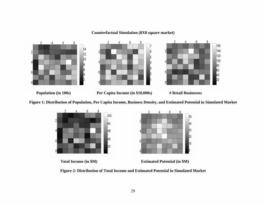
Counterfactual Simulations

To illustrate our results using counterfactual simulations, we generate a hypothetical 8 ×

8 square market with 64 locations, with a randomly generated distribution of population, per

capita income, and retail business in these locations. In Figure 1, we depict the distribution of

these variables in the market. We use our estimation results to determine the location choice

probabilities of different store formats for the case in which four firms can enter the market. In

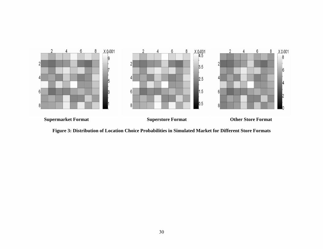
Figure 2, we portray how firms’ optimal strategies transform the distribution of total income of

consumers (Pop × PCI) into the potential across locations, and in Figure 3, we depict these

strategies (i.e., probability distributions of location choices for different formats). The four firms

that enter the market include one SMF, one SSF, and two OSF. The firms choose their locations

according to the predictions of the static entry model. In Figure 4, we show the characteristics of

the market locations and the locations chosen by these stores.

The model estimates enable us to predict the location choice strategy of a new entrant

that can observe the chosen locations of the existing firms. In our hypothetical market, after the

four stores have entered, we assume a previously unexpected increase in the unobserved

exogenous demand ( mξ ), so that a fifth firm can enter the market. If that fifth firm is a SMF

entrant, we can compare the predicted location choice when the agglomeration effects are

modeled versus when the model ignores them and find that the entrant chooses to colocate with

the SSF so it can reap the benefits of format agglomeration at that location while still

maintaining a comfortable distance from the SMF incumbent (Figure 5, Panel a). Ignoring the

25

benefits of agglomeration would cause an erroneous prediction for the entrant’s location choice

(Figure 5, Panel b). Thus, modeling the differentiation–agglomeration trade-off is critical for

firms to arrive at accurate predictions about their location choice strategies for given market

conditions.

Conclusion

Retail store chains looking for growth opportunities must make crucial entry and location

decisions. We estimate a structural model of entry and location choice to investigate the nature of

competition among different grocery store formats as a function of their locations. As we show,

previous research in this area, which focuses only on the differentiation benefit of locating far

apart, fails to capture the agglomeration benefits of colocation and therefore cannot explain

observed colocations. By decomposing firm profits, typically modeled in a reduced form in

structural entry and location literature, into the constituent elements of customer location choice

and competitive effects, we disentangle the differentiation–agglomeration trade-off.

In particular, we find support for agglomeration benefits from both format and store

agglomeration, in support of both the economies of scope and hold-up avoidance arguments

behind agglomeration. Furthermore, consumers suffer high travel costs, and the extant of

competition decreases dramatically with distance. Ignoring agglomeration effects significantly

biases estimates of travel costs and the extent of competition. Intraformat competition reduces

profits at twice the rate of interformat competition, and our policy simulations show that

disentangling the agglomeration–differentiation trade-off is critical if firms want to arrive at the

correct entry and location decisions.

We conclude with a discussion of some of the limitations of our research and some

suggestions for further work. Although our focus is on the choice of a geographic location,

26

researchers could apply a similar approach to choice of location in product spaces. Therefore, our

approach can be extended to the development of new products or new services.

We use Seim’s (2006) approach, which requires a unique equilibrium and shows

parametric conditions where the uniqueness condition is satisfied. Research using two-step

approaches (Bajari et al. 2006; Ellickson and Misra 2007) sidesteps the multiple equilibria issue,

but they are not efficient. Recently, Su and Judd (2007) developed mathematical programming

with equilibrium constraints approaches that are both efficient and avoid the multiple equilibria

problem; it therefore would be worthwhile to try this alternative approach to the problem

discussed herein.

Finally, we treat entry and location decisions within a static equilibrium framework, even

though these decisions are made over time and therefore might be better modeled in a dynamic

framework. This modeling approach would require richer data (i.e., timing of entry), as well as

richer modeling frameworks to solve the dynamic game. These interesting issues await

additional research.

References

Aradillas-Lopoez, A. (2005), “Semiparametric Estimation of a Simultaneous Game with

Incomplete Information,” Working paper.

Arentze, T.A., O. H. Oppewal, and H.J.P. Timmermans (2005), “A Multipurpose Shopping Trip

model to Assess Retail Agglomeration Effects,” Journal of Marketing Research, 42

(February), 109-115.

Bajari, P., H. Hong, J. Krainer, and D. Nekipelov (2006), “Estimating Static Models of Strategic

Interactions,” National Bureau of Economic Research, Working Paper Series.

Bester, H (1998), “Quality Uncertainty Mitigates Product Differentiation,” RAND Journal of

Economics, 29 (Winter), 828-844.

27

Bresnahan, T., and P. Reiss (1991), “Entry and Competition in Concentrated Markets,” Journal

of Political Economy, 99, 977-1009.

Chan, T. Y., V. Padmanabhan, and P. B. Seetharaman (2006), “An Econometric Model of

Location and Pricing in the Gasoline Market,” Journal of Marketing Research,

Forthcoming.

Ciliberto, F. and E. Tamer (2006), “Market Structure and Multiple Equilibria in Airline

Markets,” Working Paper.

DeLisle, J.R. (2005), “Shopping Center Classifications: Challenges and Oppurtunities,” ICSC

Working Paper Series.

Duan, A.J. and C. F. Mela (2007), “The Role of Spatial Demand on Outlet Location and

Pricing,” Working paper.

Dudey, M. (1990), “Competition by Choice: The Effect of Consumer Search on Firm Location

Decisions,” The American Economic Review, 80 (5), 1092-1104.

Ellickson, P.B., and S. Misra (2007), “Supermarket Pricing Strategies,” Working paper.

Fischer, J.H., and J.E. Harington (1996), “Product Variety and Firm Agglomeration,” RAND

Journal of Economics, 27, 281-309.

Jia, P. (2007), “What Happens When Wal-Mart Comes to Town: An Empirical Analysis of the

Discount Retailing Industry,” Working paper.

Mazzeo, M. (2002), “Product Choice and Oligopoly Market Structure,” RAND Journal of

Economics, 33, 221-242.

Merrill Lynch, company reports, 2007.

Seim, K. (2006), “An Empirical Model of Firm Entry with Endogenous Product-Type Choices,”

RAND Journal of Economics, 37 (3), 619-640.

Stahl, K. (1982), “Differentiated Products, Consumer Search, and Locational Oligopoly,” The

Journal of Industrial Economics, 31 (1-2), 97-113.

Su, C., and K. L. Judd (2007), “Constrained Optimization Approaches to Estimation of

Structural Models,” Working paper

Thomadsen, R. (2007), “Product Positioning and Competition: The Role of Location in the Fast

Food Industry,” Marketing Science, Forthcoming.

Watson, R. (2007), “Product Variety and Competition in the Retail Market for Eyeglass,”

Working paper.

28

Wernerfelt, B. (1994), “Selling Formats for Search Goods,” Marketing Science, 13 (3), 298-309.

Wolinsky, A. (1983), “Retail Trade Concentration Due to Consumers’ Imperfect Information,”

The Bell Journal of Economics, 14 (1), 275-282.

Zhu, T. and V. Singh (2007), “Spatial Competition with Endogenous Location Choices: An

Application to Discount Retailing,” Working paper.

29

Counterfactual Simulation (8X8 square market)

Population (in 100s) Per Capita Income (in $10,000s) # Retail Businesses

Figure 1: Distribution of Population, Per Capita Income, Business Density, and Estimated Potential in Simulated Market

Total Income (in $M) Estimated Potential (in $M)

Figure 2: Distribution of Total Income and Estimated Potential in Simulated Market

30

Supermarket Format Superstore Format Other Store Format

Figure 3: Distribution of Location Choice Probabilities in Simulated Market for Different Store Formats

31

SSF Location 1 P = 756, R = 84, I = $49,000

Location 2 P = 350, R = 64, I = $,40,800

Location 3 P = 274, R = 77, I = $31,000

Location 4 P = 620, R = 65, I = $31,000

P = 599, R = 95, I = $42,300

Location 6 P = 841, R = 68 I = $64,800

Location 7 P = 920, R = 89 I = $64,800

Location 8 P = 723, R = 66 I = $54,400

Location 9 P = 838, R = 45, I = $34,000

P = 499, R = 70, I = $18,600

P = 383, R = 93, I = $73,400

P = 590, R = 108, I = $48,000

P = 547, R = 170, I = $42,900

P = 490, R = 83, I = $39,400

P = 419, R = 55 I = $22,700

P = 399, R = 87 I = $66,600

OSF Location 17 P = 689, R = 91, I = $54,000

P = 1,305, R = 76 I = $18,700

P = 916, R = 131 I = $26,200 P = 667, R = 148,

I = $68,000

P = 367, R = 119 I = $55,700

P = 988, R = 124 I = $21,900

P = 825, R = 66 I = $67,700

P = 944, R = 69 I = $58,500

Location 25 P = 206, R = 69, I = $44,000

P = 1,030, R=121 I = $50,000

P = 1,165, R= 64, I = $54,900

P = 920, R = 141, I = $48,800

P = 839, R = 98, I = $66,000

P= 1,083, R = 38 I = $32,800

P = 1,589, R = 63 I = $68,500

P = 799, R = 103, I = $52,000

SMF OSF Location 33 P = 221, R = 138, I = $23,700

P = 1,478, R = 88 I = $38,100

P = 914, R = 119 I = $61,800

P = 927, R = 82, I = $41,300

P = 1,079, R=140 I = $46,000

P = 388, R = 43, I = $19,100

P = 1,103, R = 58 I = $49,800

P = 1,128, R = 75 I = $56,000

Location 41 P = 450, R = 78 I = $29,800

P = 1,087, R = 33 I = $62,500

P = 661, R = 44, I = $20,600

P = 1,349, R = 33 I = $63,100

P = 1,120, R = 71 I = $64,200

P = 662, R = 92 PCI = $37,300

P = 675, R = 78 I = $51,000

P = 1,250, R = 83 I = $36,000

Location 49 P = 879, R = 58 I = $41,000

P = 579, R = 109, I = $65,000

P = 953, R = 73 I = $54,100

P = 420, R = 134, I = $39,200

P = 1,037, R = 40 I = $25,200

P = 915, R = 43 I = $52,300

P = 1,330, R=144 I = $66,300

P = 1,194, R = 58 I = $21,200

Location 57 P = 340, R = 48 I = $31,000

P = 890, R = 74 I = $41,000

P = 870, R = 81 I = $54,500

P = 604, R = 118, I = $51,500

P = 845, R = 48, I = $55,900

P = 810, R = 109 I = $22,100

P = 620, R = 63 I = $48,600

P = 1,030, R = 90 I = $41,000

Notes: P, population; R, # retail businesses, I, per capita income, SMF, supermarket, SSF, superstore, OSF, other store format.

Figure 4: Equilibrium Store Locations in the Simulated Market

32

Super-store

Entrant Super-market

Other

Super-market Other

Figure 5(a): Entrant’s Location when Model Includes Agglomeration Effects

Super-store

Other

Super-market

Entrant Super-market

Other

Figure 5(b): Entrant’s Location when Model Does Not Include Agglomeration Effects

33

Table 1: New Store Openings for Retailers

SPECIALITY 2001 2002 2003 2004 2005 2006 2007 (proj.)Abercrombie 137 106 103 88 63 104 95 American Eagle 62 28 52 41 23 56 40 Ann Taylor 60 46 64 90 86 76 70 Bombay Company 11 3 49 31 -4 -46 -42 Buckle 21 9 12 11 11 16 16 Claire's Stores -144 48 28 31 66 90 85 Coach 19 23 20 18 25 29 40 GAP 249 20 -95 -28 59 -3 0 Pacific Sunwear 129 73 86 113 115 100 95 Sharper Image 12 18 22 26 15 0 0 Talbot’s 78 86 91 72 34 67 50 Total 634 460 432 493 493 489 449 ANCHOR Dillard's 1 -5 -5 1 1 5 5 Federated 18 -3 4 0 486 -80 5 JCPenney -36 -14 17 1 -60 21 40 May’s 18 4 1 57 -501 0 0 Nordstrom 15 11 13 2 7 2 5 Total 16 -7 30 61 -67 -52 55 COMMUNITY Cost Plus 48 0 29 33 33 17 23 Dollar General 540 573 587 620 609 525 -175 Dress Barn 31 34 18 4 -65 67 44 Family Dollar 452 475 411 439 432 275 335 Men's Wearhouse 29 9 41 4 18 25 5 Office Depot -29 8 33 69 78 108 125 Pier 1 75 100 105 79 42 -25 -10 Ross Stores 43 55 61 81 71 75 90 TJX 172 178 219 162 161 101 104 Total 1,361 1,432 1,467 1,501 1,379 1,168 541 COMMUNITY/POWER ANCHORS Target 74 94 78 -245 89 98 115 Wal-Mart 315 364 372 349 352 349 260 Total 389 458 450 104 441 447 375 POWER ANCHORS BJ’s 12 10 10 7 8 10 13 Bed Bath & Beyond 80 130 103 92 88 81 90 Circuit City -5 2 -22 13 18 20 0 Costco 52 9 23 20 16 22 30 Home Depot 203 195 175 183 152 118 90 Lowe's 94 110 98 135 147 155 151 Total 436 456 387 450 429 406 374 Source: Company Reports, Merrill Lynch

34

Table 2: Average Demographics by Location With and Without Agglomeration

Store Locations

Where Nearest Rival

Is More than 2 Miles

Away

Store Locations

Where Nearest Rival

Is Within Half Mile

0–1 mile 31.47 22.52

1–3 miles 158.87 95.39 Population (× 103)

> 3 miles 209.8 259.69

0–1 mile 19.4 20.8

1–3 miles 18.9 20.0 Per capita income

(× 103) > 3 miles 20.5 19.8

0–1 mile 57.39 45.00

1–3 miles 280.12 185.73 Cumulative income

(× 106) > 3 miles 430.80 513.83

# Retail businesses 0–1 mile 97.4 121.15

1–3 miles 90.88 111.58

> 3 miles 87.57 74.44

35

Table 3: Coefficients of Variation by Markets

With and Without Agglomeration

Store Locations Where

Nearest Rival Is More

than 2 Miles Away

Average (Std. Dev.)

Store Locations

Where Nearest Rival

Is Within Half Mile

Average (Std. Dev.)

0–1 mile 0.1067 (0.1841) 0.2011 (0.1972)

1–3 miles 0.3756 (0.1999) 0.4189 (0.1688) Population (× 103)

> 3 miles 0.4977 (0.1941) 0.5133 (0.2620)

0–1 mile 0.0673 (0.1239) 0.1516 (0.1860)

1–3 miles 0.2686 (0.1391) 0.3137 (0.1733) Per capita income

(× 103) > 3 miles 0.3423 (0.1669) 0.3851 (0.1938)

0–1 mile 0.1163 (0.1989) 0.2498 (0.2587)

1–3 miles 0.5013 (0.2544) 0.5604 (0.2091) Cumulative income

(× 107) > 3 miles 0.7168 (0.2946) 0.7338 (0.3583)

# Retail businesses 0–1 mile 0.1537 (0.2899) 0.0780 (0.2200)

1–3 miles 0.5664 (0.4478) 0.6027 (0.4207)

> 3 miles 0.6684 (0.4042) 0.7690 (0.3684)

Table 4: Summary Statistics of Data

Total Number of Markets 146

Mean Std. Dev. Number of stores in a market 4.6 2.5

Market radius (miles) 5.85 1.89 Number of locations in a market 29.74 27.66

Population in a location 951.3 618.4 Per capita income in a location 17,859 9,537

Retail establishments in a zip code 81.23 69.98

36

Table 5: Store Interaction Ratings for Different Store Chains

Store chain

A.

Average Rating

B.

Rating after Controlling

for Distance

B 7.75 15.23

C 7.31 9.78

D 5.60 8.23

E 5.16 8.12

F 3.68 5.71

G 4.82 5.20

H 4.24 4.94

I 3.49 4.60

J 3.41 4.34

K 2.48 3.46

L 1.94 2.12

37

Table 6: Results with the Assumption of Homogeneous Firms

A. Without Agglomeration

Effect

B. With Agglomeration

Effect

Consumers' Shopping Behavior

# Retail businesses (100) 0.4483 (0.0664) 0.4241 (0.0867)

Distance (in miles) -0.3139 (0.0589) -0.4637 (0.0577)

Store agglomeration effect - - 0.2660 (0.0525)

Store Profitability

ln(Potential) 1.1375 (0.1608) 1.1623 (0.1696)

ln(# Rivals in 1mi.) -3.3468 (0.1637) -3.8907 (0.1337)

ln(# Rivals in 1-3mi.) -0.2056 (0.0412) -0.3341 (0.0547)

ln(# Rivals in 3-5mi.) -0.0369 (0.0381) -0.0281 (0.0558)

Mean Exgns unobv, μ -6.2772 (0.3719) -5.9701 (0.3826)

Std Exgns unobv, σ 0.6864 (0.0529) 0.6983 (0.0552)

Negative log-likelihood 2166.61 2161.34

Table 7: Reduction in Chain A’s Profits Because of a New Entrant Within 1 Mile

Estimated Reduction

in Profits

When Agglomeration Effect is

Not Modeled

(a)

When Agglomeration Effect is

Modeled

(b)

Average 65.6% 60.4%

Maximum 75.0% 73.0%

Minimum 36.7% 23.4%

38

Table 8: Asymmetric Competition Among Three Store Formats

SMF –

Notes: Supermarket format; SSF – Superstore format; NSF – Niche store format; (SMF-SMF)0 – Competition between two

supermarket stores that are within 1 mile of each other; (SMF-SMF)1 - Competition between two supermarket stores that are 1-3 miles

from each other; Similarly others.

*For SMF, we normalize the intercept to 0 for identification.

Consumers' shopping behavior # Retail Businesses (100) 0.4410 (0.0623) Distance in miles -0.4181 (0.0715) Store agglomeration effect 0.2151 (0.0743) Format agglomeration effect 0.0765 (0.0218) Store profitability Ln(Potential) 1.1325 (0.0741) Intra-format competition (SMF-SMF)0 -5.1874 (0.2480) (SSF-SSF)0 -4.6672 (1.4621) (OSF-OSF)0 -3.4253 (0.3891) (SMF-SMF)1 -0.3579 (0.0937) (SSF-SSF)1 -0.5191 (0.1932) (OSF-OSF)1 -0.2845 (0.0923) Inter-format competition (SMF-SSF)0 -2.3126 (0.2841) (SMF-OSF)0 -0.7733 (0.1482) (SSF-OSF)0 -2.3966 (0.2891) (SMF-SSF)1 0.0060 (0.0475) (SMF-OSF)1 0.1057 (0.1215) (SSF-OSF)1 -0.2743 (0.0389) SSF intercept* -0.7033 (0.0681) μ -3.5248 (0.2984) OSF intercept -0.5689 (0.0314) σ 0.6810 (0..0571) Negative log-likelihood 2769.70

39

Table 9: Reduction in Chain A’s Profits Because of a New Entrant Within 1 Mile

Reduction in Profits SMF Entrant SSF Entrant OSF Entrant

Average 77.2% 54.1% -17.0% Maximum 82.6% 64.5% 1.8% Minimum 44.1% 16.5% -41.2%