a study of elliptical vibration cutting in … study of elliptical vibration cutting in ultra...

A STUDY OF ELLIPTICAL VIBRATION CUTTING IN

ULTRA PRECISION MACHINING

ZHANG XINQUAN

(B. Eng., Harbin Institute of Technology)

A THESIS SUBMITTED

FOR THE DEGREE OF DOCTOR OF PHILOSOPHY

DEPARTMENT OF MECHANICAL ENGINEERING

NATIONAL UNIVERSITY OF SINGAPORE

2012

Acknowledgement

i

Acknowledgement

Firstly, I would like to express my deepest and earnest appreciation to my

supervisor, Associate Professor A. Senthil Kumar, for his continuous strong support,

untiring efforts, excellent supervision and patient guidance. He does not only provide

me plenty of knowledge regarding my research, but also share with me his wisdom,

insight and life attitude in the past few years. It is really my honor to achieve the

guidance from him during my PhD career.

Also, I would like to show my sincere gratitude to my co-supervisor, Professor

Mustafizur Rahman for his uninterrupted guidance, unwavering support and

encouragement throughout my study. He has constantly provided me with valuable

assistance and advice to improve both my academic research and daily life.

Special thanks to Dr. Liu Kui and Dr. Nath Chandra from Singapore Institute of

Manufacturing Technology for his continuous financial and scholastic support for my

research project. I would like to express my deep appreciation to my fiancée, my

family, and my friends for their unselfish love, encouragement, and sacrifices

throughout my life.

Last but not least, thanks to the staffs of AML: Mr. Nelson Yeo Eng Huat, Mr.

Neo Ken Soon, Mr. Tan Choon Huat, Mr. Lim Soon Cheong and Mr. Wong Chian

Loong for their time and support in operating the machines and instruments for my

experiments. Also thanks to my labmates and friends: Dr. Yu Deping, Dr. Arif, Dr.

Asma and Dr. Wang Jingjing for their academic help and inspiration.

Table of Contents

ii

Table of Contents

Acknowledgement ......................................................................................................... i

Table of Contents .......................................................................................................... ii

Summary ...................................................................................................................... vi

List of Tables ............................................................................................................. viii

List of Figure s .............................................................................................................. ix

Abbreviations ............................................................................................................. xvi

Nomenclature ............................................................................................................ xvii

Chapter 1: Introduction ..........................................................................................1

1.1 Vibration-assisted machining (VAM) ................................................................. 1

1.2 Elliptical vibration cutting (EVC) ....................................................................... 2

1.3 Main objectives of this study ............................................................................... 3

1.4 Organization of this dissertation .......................................................................... 4

Chapter 2: Literature review ..................................................................................6

2.1 Principle of VAM ................................................................................................ 6

2.1.1 Principle of CVC ........................................................................................ 6

2.1.2 Principle of EVC ........................................................................................ 8

2.2 EVC systems ..................................................................................................... 13

2.2.1 Resonant EVC systems ............................................................................ 13

2.2.2 Non-resonant EVC systems ...................................................................... 16

2.3 Benefits of the EVC method ............................................................................. 18

2.3.1 Smaller cutting force values ..................................................................... 18

2.3.2 Improved surface finish ............................................................................ 20

2.3.3 Extended tool life ..................................................................................... 23

Table of Contents

iii

2.3.4 Improved form accuracy and burr suppression ........................................ 25

2.4 Analytical studies of EVC ................................................................................. 27

2.4.1 Force models ............................................................................................ 27

2.4.2 Surface generation and critical speed ratio ............................................... 29

2.4.3 FEM and MD analysis .............................................................................. 30

2.5 Concluding remarks .......................................................................................... 32

Chapter 3: Experimental investigation of transient cutting force in EVC ...........34

3.1 Characteristics of the EVC process ................................................................... 35

3.1.1 Transient thickness of cut ......................................................................... 35

3.1.2 Friction reversal process in the EVC process ........................................... 38

3.2 Experimental details .......................................................................................... 42

3.3 Results and analysis ........................................................................................... 46

3.3.1 Effect of speed ratio ................................................................................. 46

3.3.2 Effect of tangential amplitude .................................................................. 49

3.3.3 Effect of thrust amplitude ......................................................................... 51


Chapter 4: Modeling of transient cutting force for the EVC method ..................55

4.1 Development of the force model ....................................................................... 56

4.1.1 Transient thickness of cut ......................................................................... 56

4.1.2 Transient shear angle and transition characteristic of friction reversal .... 56

4.1.3 Transient cutting force components ......................................................... 65

4.2 Verification for the proposed model ................................................................. 67

4.2.1 Calibration for the parameters .................................................................. 67

4.2.2 Validation for the developed model ......................................................... 70

4.3 Concluding Remarks ......................................................................................... 73

Chapter 5: Experimental and analytical studies of surface generation in EVC ...75

Table of Contents

iv

5.1 Experimental study using the SCD tool ............................................................ 76

5.1.1 Experimental setup ................................................................................... 76

5.1.2 Results and analysis .................................................................................. 77

5.2 Development of the surface generation model considering tool edge radius .... 81

5.3 Experimental verification .................................................................................. 88

5.3.1 Experimental design ................................................................................. 88

5.3.2 Experimental results ................................................................................. 90


Chapter 6: Ultrasonic EVC of hardened stainless steel using PCD tools ............94

6.1 Experimental setup and procedures ................................................................... 95

6.2 Results and analysis ........................................................................................... 99

6.2.1 Effects of cutting parameters on force components ................................. 99

6.2.2 Effects of cutting parameters on tool wear ............................................. 101

6.2.3 Effects of cutting parameters on chip formation .................................... 103

6.2.4 Effects of cutting parameters on surface roughness ............................... 105

6.2.5 Evaluation test for obtaining mirror quality surface .............................. 109

6.3 Concluding remarks ........................................................................................ 112

Chapter 7: Tool wear suppression mechanism for machining steel using diamond

with the VAM method ...............................................................................................114

7.1 Modeling of cutting energy consumption in VAM ......................................... 115

7.2 Measurement of the workpiece temperature ................................................... 123

7.3 Tool wear suppression mechanism in VAM ................................................... 128

7.3.1 Experimental investigation ..................................................................... 128

7.3.2 Contamination of the tool-workpiece interface ...................................... 132

7.3.3 Generation of iron oxide on the freshly machined surface .................... 134

7.4 Concluding remarks ........................................................................................ 138

Table of Contents

v

Chapter 8: Main conclusions and recommendations .........................................140

8.1 Main contributions .......................................................................................... 140

8.2 Recommendations for future work .................................................................. 143

References ..................................................................................................................146

Publication list ...........................................................................................................153

Summary

vi

Summary

In the field of precision manufacturing industry, vibration-assisted machining

(VAM) has already been demonstrated as a well-known cost-effective method for

machining various materials with superior cutting performance compared with

conventional cutting (CC) method. As a novel 2D VAM method, elliptical vibration

cutting (EVC) has received a lot of attention for its better machining performance

especially in machining brittle and hard materials. However, compared to the

conventional vibration cutting (CVC) method, very few in-depth experimental and

analytical studies have been conducted on transient cutting force, surface generation

and tool wear mechanism for the more advanced EVC method.

This study has been carried out in three phases. In the first phase, as cutting

force is considered as the most important indicator of machining state and quality, in

order to investigate the transient cutting force, a novel method is proposed to realize

the low-frequency EVC motion by G-code programming and axis motion control of

an ultraprecision machine tool. Based on this method, the transient cutting force in the

EVC process is experimentally investigated under different cutting and vibration

parameters. Then, an analytical force model is developed for in-depth understanding

of the transient cutting mechanics and for accurate prediction of the transient cutting

force. In this model, transient thickness of cut and transient shear angle are considered

and calculated, and each EVC cycle is divided into three consecutive zones (i.e. CC-

like kinetic-friction zone, static-friction zone and reverse kinetic-friction zone) based

on the variation of friction modes. Experimental verification is also carried out to

justify the validity of the developed cutting force model.

Summary

vii

In the second phase, surface generation along nominal cutting direction in EVC is

experimentally investigated by conducting a series of grooving tests using a single

crystal diamond tool. Then, in order to better understand the surface generation

process, a more comprehensive calculation method is developed for determining the

theoretical roughness considering the edge radius. The comparison between

experimental and predicted roughness shows that the proposed model could predict

much more accurate surface roughness than the prevailing model, in which the tool

edge radius is not considered.

In the third phase, commercial PCD tools are used to machine hardened stainless

steel with the ultrasonic EVC method, and the effects of conventional machining

parameters on different output parameters (including cutting force, tool wear, chip

formation, and surface roughness) are experimentally investigated. It is found that

wear of diamond tools is significantly reduced by applying VAM, and nominal

cutting speed has the strongest influence on the tool wear and the surface roughness.

Then, an in-depth study is conducted by modeling the cutting energy consumption

based on the obtained transient cutting force and measuring the workpiece

temperature to find out the reason for the phenomenon. Both the theoretical and

experimental results show that the reduced diamond tool wear in VAM of steel is not

caused by the reduced heat generation and tool/workpiece temperature which is

claimed by previous researchers. Finally, based on investigation and understandings

of graphitization mechanism of diamond, two main reasons are suggested to be

responsible for the significantly reduced wear rate of diamond tools in VAM of steel:

i) contamination of the tool/workpiece interface, and ii) generation of iron oxide.

List of Tables

viii

List of Tables

Table 3.1. Cutting and vibration conditions of the orthogonal EVC tests. .................. 45

Table 4.1. Cutting and vibration conditions for the orthogonal CC test. ..................... 68

Table 5.1. Conditions of the grooving test ................................................................... 77

Table 5.2. Conditions of the grooving test using the EVC method. ............................ 89

Table 6.1 Workpiece material composition ................................................................. 96

Table 6.2 The EVC test conditions used during face turning ...................................... 98

Table 7.1. Conditions for measurement of the workpiece temperature. .................... 126

Table 7.2. Conditions for machining steel using PCD tools with CC and VAM

methods. ..................................................................................................................... 129

Table 7.3. Wear rates of diamond tools for turning mild steel using CC method (10-6

mm2mm-2) (Thornton and Wilks, 1979). ................................................................... 132

List of Figures

ix

List of Figures

Figure 2.1. Schematic illustration of the CVC process. ................................................. 7

Figure 2.2. Schematic illustration of the EVC process: (a) 2D view, (b) 3D view. ...... 9

Figure 2.3. Ideal surface generation process in EVC................................................... 12

Figure

2.4. Two generations of ultrasonic resonant EVC systems and their vibration

modes: (a) 20 kHz (Shamoto et al., 2002), (b) 40 kHz (Suzuki et al., 2007a)............. 15

Figure

2.5. 3D ultrasonic resonant EVC system and its vibration modes (Suzuki et al.,

2007b). ......................................................................................................................... 16

Figure

2.6. Non-resonant EVC system developed at Pusan University (Ahn et al.,

1999). ........................................................................................................................... 17

Figure

2.7. Non-resonant EVC system developed at North Carolina State University

(Brehl and Dow, 2008). ............................................................................................... 17

Figure

2.8. Principal and thrust components of the measured cutting force for: (a) CC,

(b) CVC , (c) EVC (0.4 Hz), (d) EVC (6 Hz) (Shamoto and Moriwaki, 1994). ......... 19

Figure

2.9. Comparison of average cutting forces for: (a) ultrasonic CVC and

ultrasonic EVC methods (Shamoto and Moriwaki, 1999), (b) CC (“ordinary cutting”),

ultrasonic CVC and ultrasonic EVC methods (Ma et al., 2004). ................................. 20

Figure

2.10. Comparison of surface roughness against cutting distance for CVC and

EVC (Shamoto et al., 1999a). ...................................................................................... 21

Figure

2.11. Comparison of the surfaces finished by two cutting methods (CC and

EVC) for different brittle materials: (a) sintered tungsten carbide, (b) zirconia

ceramics, (c) calcium fluoride, and (d) glass (Suzuki et al., 2004). ............................. 23

List of Figures

x

Figure

2.12. SEM photographs of cutting edges of worn diamond tools: (a) after CVC

of steel for 1000m, and (b) after EVC of steel for 2800m (Shamoto and Moriwaki,

1999). ........................................................................................................................... 24

Figure

2.13. Comparison of cutting performance between the CC and EVC methods

(Nath et al., 2009c)....................................................................................................... 25

Figure

2.14. Cutting edges of diamond tools used for planing tungsten alloys with: (a)

after CC of 1.08 m, and (b) after EVC of 1.35 m (Suzuki et al., 2007a). .................... 25

Figure

2.15. Influence of the three cutting methods (CC, CVC and EVC) on the shape

error (Ma et al., 2004). ................................................................................................. 26

Figure 2.16. Height of burrs for the CC, CVC and EVC methods (Ma et al., 2005). . 27

Figure

2.17. (a) Redrawn sketch of the EVC force model, (b) Simulated and

experimental transient cutting forces (Shamoto et al., 2008). ..................................... 28

Figure

2.18. Photographs of the machined surfaces of sintered tungsten carbide for

different values of speed ratios: (a) 0.075 (Rs < 0.12837), (b) 0.131 (Rs > 0.12837)

(Nath et al., 2011). ....................................................................................................... 30

Figure

2.19. Chip formation and stress distribution simulated in one vibration cycle in

EVC (Amini et al., 2010). ............................................................................................ 31

Figure

3.1. 2D view of the EVC process at different time instants: (a) before the tool

edge passes the (TOCt)m point, (b) after the tool edge passes the (TOCt)m point. ....... 36

Figure 3.2. Schematic illustration of the CC process................................................... 39

Figure

3.3. Force and velocity relationships after the tool passes the friction reversal

point in the EVC process. ............................................................................................ 40

Figure

3.4. Schematic illustration of (a) transient kinetic-friction angle, and (b)

transient shear angle in an EVC cycle. ........................................................................ 41

List of Figures

xi

Figure

3.5. Illustration of the procedures for generating the low-frequency EVC

motion. ......................................................................................................................... 43

Figure 3.6. Illustration of the experimental set-up for the low-frequency EVC tests. . 44

Figure 3.7. Microscope photograph (X50) of the flat nose diamond tool. .................. 44

Figure 3.8. Experimental set-up for the orthogonal EVC tests. ................................... 45

Figure

3.9. The effect of speed ratio on (a) the transient cutting force components, (b)

the maximum resultant cutting force. .......................................................................... 47

Figure 3.10. The effect of speed ratio on the values of (a) TOCt, (b) (TOCt)m. ........... 48

Figure 3.11. The effect of speed ratio on the value of friction reversal time. .............. 49

Figure

3.12. The effect of tangential amplitude on (a) the transient cutting force

components, (b) the maximum resultant cutting force. ............................................... 50

Figure

3.13. The effect of tangential amplitude on the values of (a) TOCt, (b) (TOCt)m,

(c) friction reversal time............................................................................................... 51

Figure

3.14. The effect of thrust amplitude on (a) the transient cutting force

components, (b) the maximum resultant cutting force. ............................................... 52

Figure

3.15. The effects of thrust amplitude in the EVC process on the values of (a)

TOCt, (b) (TOCt)m, (c) friction reversal time. .............................................................. 53

Figure

4.1. Slip-line fields and force relationships for a single EVC cycle in: (a) CC-

like kinetic-friction zone, (b) Reverse kinetic-friction zone. ....................................... 59

Figure

4.2. Velocity diagrams for a single EVC cycle in: (a) CC-like kinetic-friction

zone, (b) Static-friction zone, (c) Reverse kinetic-friction zone. ................................. 60

Figure

4.3. Schematic sketch of the three consecutive friction zones in an EVC cycle

versus: (a) tool velocity direction, (b) tool location. .................................................... 63

List of Figures

xii

Figure

4.4. Example of transient shear angle for a cutting cycle in orthogonal EVC

process at the conditions: 0o tool rake angle, 0.094 mm/min nominal cutting speed,

vibration amplitude (a=20 µm, b=5 µm), 0.25 Hz frequency, 90o phase shift. ........... 64

Figure

4.5. Flow chart of the calculation procedures for the analytical EVC force

model............................................................................................................................ 67

Figure

4.6. Experimental results for the CC process: (a) Cutting force components, (b)

Microscope photograph (X450) of the formed chip. ................................................... 69

Figure

4.7. Experimental and predicted maximum transient resultant cutting force

with different speed ratios. ........................................................................................... 71

Figure

4.8. Experimental and predicted transient cutting force components for an

EVC cycle. ................................................................................................................... 73

Figure

5.1. Microscope photographs (×1000) of the grooves with different nominal

cutting speeds under the EVC method. Condition: b= 2 µm. ...................................... 78

Figure

5.2. Example of surface analysis by a white light interferometer. (a) Contour

image of the groove bottom, (b) Surface profile along the nominal cutting direction.

Conditions: vc= 6 m/min, b= 2 µm............................................................................... 79

Figure

5.3. Experimental and predicted roughness values along nominal cutting

direction with different nominal cutting speeds. Conditions: (a) b= 2 µm, (b) b= 1 µm.

...................................................................................................................................... 80

Figure 5.4. Schematic cross-section view of tool geometry. ....................................... 82

Figure

5.5. Illustration of the surface generation for the EVC process considering the

round tool edge. ........................................................................................................... 83

Figure

5.6. Flow chart for calculating the analytical surface considering tool edge

radius. ........................................................................................................................... 86

List of Figures

xiii

Figure

5.7. (a) Simulated surface profiles along the nominal cutting direction

considering tool edge radius for the EVC process, (b) Theoretical roughness versus

tool edge radius. Conditions: 3 m/min nominal cutting speed; circular vibration with 2

µm amplitude; 38.87 kHz vibration frequency. ........................................................... 87

Figure 5.8. Experimental setup with the elliptical vibrator. ........................................ 88

Figure 5.9. AFM analysis of the PCD tool edge indentation. ...................................... 90

Figure

5.10. Microscope photographs (×1000) of the machined grooves under the

EVC method on the workpieces made of: (a) Aluminum alloy, (b) Hardened steel. .. 90

Figure

5.11. Surface roughness measurement using the white light interferometer.

Condition: 6 m/min nominal cutting speed. ................................................................. 91

Figure

5.12. Experimental and predicted roughness along nominal cutting direction

with different nominal cutting speeds. ......................................................................... 92

Figure

6.1. Experimental setup with the elliptical vibrator on the ultraprecision

machine for the EVC test. ............................................................................................ 96

Figure

6.2. Schematic illustration of: (a) machining area, (b) 3D view of the turning

process.......................................................................................................................... 98

Figure

6.3. Effects of machining parameters on cutting force components: (a) nominal

DOC (nr = 15 rpm, fr = 10 µm/rev), (b) feed rate (nr = 15 rpm, DOC = 10 µm), (c)

nominal cutting speed (fr = 5 µm/rev, DOC = 10 µm). .............................................. 100

Figure

6.4. Microscope (100× and 500 ×) photographs of the flank wear of PCD tools:

(a) DOC = 10 µm, fr = 5 µm/rev, nr = 45 rpm, Lc= 110 m, (b) DOC = 10 µm, fr = 5

µm/rev, nr = 30 rpm, Lc= 110 m, (c) DOC = 4 µm, fr = 10 µm/rev, nr = 15 rpm, Lc= 55

m, (d) DOC = 10 µm, fr = 10 µm/rev, nr = 15 rpm, Lc= 55 m, (e) DOC = 10 µm, fr =

7.5 µm/rev, nr = 15 rpm, Lc= 73 m. ............................................................................ 103

List of Figures

xiv

Figure

6.5. SEM (250×) photographs of the curled chips with four different cutting

conditions in the EVC test (DOC=10 µm): (a) nr = 45 rpm, fr = 5 µm/rev, (b) nr = 30

rpm, fr = 5 µm/rev, (c) nr = 15 rpm, fr = 5 µm/rev, (d) nr = 15 rpm, fr = 7.5 µm/rev. . 104

Figure

6.6. Effects of machining parameters on surface roughness values: (a) nominal


spindle speed (fr = 5 µm/rev, DOC = 10 µm). ........................................................... 106

Figure

6.7. Microscope photographs (500×) of the machined surfaces at three

different spindle speeds (DOC = 10 µm, fr = 5 µm/rev): (a) nr = 15 rpm, (b) nr = 30

rpm, (c) nr = 45 rpm. .................................................................................................. 108

Figure

6.8. AFM scan of the machined surface in the EVC test (DOC = 10 µm, fr = 5

µm/rev, nr = 45 rpm): (a) overview surface profile (90 µm × 90 µm), (b) measured in

the feed direction, (c) measured in the nominal cutting direction. ............................ 109

Figure

6.9. Machined surface on hardened stainless steel using a PCD tool with the

EVC technology (DOC = 10 µm, fr = 2.5 µm/rev, nr = 15 rpm). ............................... 110

Figure

6.10. Measurement results of surface roughness for the machinined surface.

.................................................................................................................................... 111

Figure

6.11. Microscope photographs (100× and 500 ×) of the worn PCD tool after

the evaluation EVC test on the hardened steel (DOC = 10 µm, fr = 2.5 µm/rev, nr = 15

rpm). ........................................................................................................................... 112

Figure 7.1. Maximum resultant cutting force in the CC and VAM processes. .......... 117

Figure

7.2. Experimental transient cutting force components in: (a) CC, (b) CVC, (c)

EVC............................................................................................................................ 118

Figure

7.3. Schematic illustration of the CVC process considering elastic deformation

and recovery. .............................................................................................................. 120

List of Figures

xv

Figure 7.4. Calculated cutting energy consumption in the CC and VAM processes. 122

Figure

7.5. Illustration of the experimental setup for measuring the workpiece

temperature: (a) schematic view, (b) physical view. ................................................. 125

Figure

7.6. Temperature variation of the workpiece under different cutting methods.

.................................................................................................................................... 127

Figure 7.7. Experimental setup for machining steel using PCD tools. ...................... 129

Figure

7.8. Microscope photographs of the tool flank faces in the three machining

processes: (a) CC, (b) CVC, (c) EVC. ....................................................................... 131

Figure

7.9. Illustration of the CC and VAM processes considering the contamination

of tool/workpiece interface. ....................................................................................... 134

Figure

7.10. Illustration of the VAM process considering the generation of iron oxide:

(a) before tool/workpiece engagement, (b) after tool/workpiece engagement. ......... 136

Figure

7.11. EDS analysis of the tool flank faces for the used PCD tools: (a) EDS

spectrums for the tool used in EVC, (b) Comparison of oxygen mass for the three

cutting methods. ......................................................................................................... 137

Abbreviations

xvi

Abbreviations

AFM Atomic force microscope

BUE Built-up edge

CC Conventional cutting

CNC Computer numerical control

CVC Conventional vibration cutting

DOC Depth of cut

EDS Energy-dispersive X-ray spectroscopy

EVC Elliptical vibration cutting

FEM Finite element method

ID Inner diameter

MD Molecular dynamics

OD Outer diameter

PCD Polycrystalline diamond

PZT Piezoelectric Transducer

SCD Single crystal diamond

SEM Scanning electron microscope

TOC Thickness of cut

VAM Vibration-assisted machining

Nomenclature

xvii

Nomenclature

Symbol Unit Description

a µm Tangential amplitude

b µm Thrust amplitude

x m x-axis coordinate

y m y-axis coordinate

t s Time

φ deg Phase shift

ω rad/s Angular frequency

cv m/min Nominal cutting speed

Rs -- Speed ratio

f Hz Vibration frequency

γ deg Tool rake angle

θ deg Transient tool velocity angle

ap µm Nominal uncut chip thickness

At s Time instant when the tool edge passes point A

Bt s Time instant when the tool edge passes point B

Ct s Time instant when the tool edge passes point C

Dt s Time instant when the tool edge passes point D

Et s Time instant when the tool edge passes point E

Ft s Time instant when the tool edge passes point F

Nomenclature

xviii

Gt s Time instant when the tool edge passes point G

Ht s Time instant when the tool edge passes point H

Pt s Time instant when the tool edge passes point P

tv -- Transient tool velocity vector

ctv -- Transient chip velocity vector relative to the tool

sv -- Transient shear velocity vector

TOCt µm Transient thickness of cut

(TOCt)m µm Maximum transient thickness of cut

τ N/m2 Shear stress

δ deg Constant angle between shear plane and resultant force

R N Resultant force

Rmax N Maximum resultant force

0t µm Uncut chip thickness in CC

ct µm Measured chip thickness in CC

w µm Width of cut

βk deg Kinetic-friction angle

βs deg Static-friction angle

Fp N Principal force along nominal cutting direction

Ft N Thrust force perpendicular to nominal cutting direction

Fs N Shear force along the shear direction

Ff N Friction force along the tool rake face

Fn N Normal force perpendicular to the tool rake face

Fns N Normal force perpendicular to the shear direction

Nomenclature

xix

cϕ deg Constant shear angle

kcϕ deg Shear angle in CC-like kinetic-friction zone

krϕ deg Shear angle in reverse kinetic-friction zone

tϕ deg Transient shear angle in EVC

sϕ deg Transient shear angle in static-friction zone

λ deg Tool clearance angle

re µm Tool edge radius

ex m x-axis coordinate of transient surface generation point

ey m y-axis coordinate of transient surface generation point

theR µm Theoretical roughness considering tool edge radius

thR µm Theoretical roughness without considering edge radius

exR µm Experimental roughness

Aet s Time instant when the tool edge passes point Ae

Cet s Time instant when the tool edge passes point Ce

Lc m Cutting length

fr mm/rev Feed rate

nr rpm Rotational speed

r mm radial distance of tool position from workpiece center

D mm Diameter at OD

d mm Diameter at ID

(vc)max m/min Maximum nominal cutting speed at OD

(vc)min m/min Minimum nominal cutting speed at ID

Nomenclature

xx

rn mm Tool nose radius

fthR µm Theoretical roughness caused by feed marks in turning

WCC J Cutting energy consumption in CC

WCVC J Cutting energy consumption in CVC

WEVC J Cutting energy consumption in EVC

CCT∆ oC Temperature rise in CC

CVCT∆ oC Temperature rise in CVC

EVCT∆ oC Temperature rise in EVC

Chapter 1

1

Chapter 1: Introduction

This chapter starts with an introduction of the vibration-assisted machining (VAM)

method and its wide application. The next section presents a brief review of the

elliptical vibration cutting (EVC) method, and the following section provides the

motivation, scope and main objectives of this study. Finally, an organizational outline

of the whole thesis is presented.

1.1 Vibration-assisted machining (VAM)

The VAM method was first introduced in 1960s and has been progressively

applied in the manufacturing industry (Kumabe et al., 1989; Skelton, 1969).

Meanwhile, a lot of experimental work for the VAM method has shown that better

cutting performance can be achieved in machining various materials compared to the

conventional cutting (CC) method. Such superior cutting performance includes

smaller cutting force (Zhou et al., 2003), better surface quality (Moriwaki and

Shamoto, 1991), longer tool life (Zhou et al., 2006) and suppression of chatter

vibration (Xiao et al., 2002), etc. It has also been demonstrated that, by employing the

VAM method, diamond tools can be applied to directly machine steel sustainably,

which is not realistic by using the CC method due to the chemical affinity between

iron and carbon atoms (Casstevens, 1983; Moriwaki and Shamoto, 1991; Paul et al.,

1996; Shamoto et al., 1999a). Moreover, the VAM method can save both

manufacturing time and cost and in turn improve the productivity compared to other

nonconventional machining methods such as electron discharge machining, laser

Chapter 1

2

technology, ELID grinding, electrochemical machining and chemical-mechanical

polishing.

Based on the number of vibration modes, two main types of VAM method can be

identified: 1D VAM (also named as CVC, i.e. conventional vibration cutting), and 2D

VAM (also named as EVC). Nowadays, CVC has been widely studied and is being

used in a broad range of machining roles, such as turning , drilling, grinding and

milling (Brehl and Dow, 2008). Compared to the CVC method, the EVC method still

belongs to the cutting edge technology, which is attracting more and more attention

recently because of its even better machining performances.

1.2 Elliptical vibration cutting (EVC)

The EVC (i.e. 2D VAM) method was first introduced in 1993 (Shamoto and

Moriwaki, 1993). During machining with the EVC method, the workpiece is fed

against the vibrating tool along the nominal cutting direction, and some piezoelectric

transducers (PZT) are arranged in a metal block to drive the tool tip to vibrate

elliptically in the EVC process. The pulling action applied by the cutting tool can

assist to pull chips away from the workpiece and lead to a reversed friction during

each cutting cycle (Shamoto and Moriwaki, 1994), and the contacting time between

the tool flank face and the workpiece is significantly reduced. Through constant

development in almost two decades, this novel method has been proved to be a

promising method in terms of almost all cutting performances compared to the CC

and CVC methods in cutting various materials, especially difficult-to-cut materials,

such as hardened steel (Shamoto and Moriwaki, 1999), glass (Shamoto et al., 1999a),

sintered tungsten carbide (Nath et al., 2009a; Suzuki et al., 2004), tungsten alloy

(Suzuki et al., 2007a), etc.

Chapter 1

3

Compared to the CVC method, studies on the novel and more advanced EVC

method are still relatively superficial, and very few experimental and analytical

studies on transient cutting force, surface generation and tool wear mechanism in the

EVC process have been conducted.

1.3 Main objectives of this study

This study aims to fulfill the following main objectives:

• To better understand the material removal mechanism in the EVC process, and

to accurately predict the transient cutting force, which is tightly correlated to

other important output machining aspects such as tool life and surface finish

quality.

• To understand the unique surface generation process, and to accurately predict

the surface roughness along the nominal cutting direction in the EVC process.

• To investigate the tool wear conditions and find out the inherent reasons for

the tool wear suppression in VAM of steel using diamond tools.

In order to achieve the above targets, the following steps have been taken in this

study:

• Developing a novel method to generate a low-frequency EVC method to make

it feasible to measure the transient cutting force.

• Experimentally investigating the variation of transient cutting force in EVC

under different cutting and vibration conditions.

• Developing and verifying an analytical force model considering three

important factors: i) the transient thickness of cut (TOC), ii) the transient shear

angle, and iii) the transition characteristic of friction reversal.

Chapter 1

4

• Developing and verifying a surface generation calculation method along the

nominal cutting direction considering tool edge radius.

• To study the feasibility of polycrystalline diamond (PCD) tools to obtain

mirror quality surface on hardened steel for die and mold applications with the

ultrasonic EVC method.

• Based on in-depth theoretical and experimental investigation, analyzing and

comparing the cutting energy consumptions and workpiece temperatures in

CC and VAM, and proposing reasonable reasons for the reduced diamond tool

wear in VAM of steel.

1.4 Organization of this dissertation

This dissertation is composed of eight chapters. Chapter 2 first introduces the

main principles of CVC and EVC, the benefits of the EVC method and the existing

relevant analytical studies. Chapter 3 presents the experimental investigation to study

the effects of various machining and vibration parameters on the transient cutting

force, in order to understand the fundamental material removal mechanism in the

EVC process. In Chapter 4, an analytical force model for the orthogonal EVC process

is developed. Then, the predicted force values calculated based on the proposed model

are compared with the experimental cutting force values at different cutting and

vibration conditions, and relevant issues observed from the results are discussed.

In Chapter 5, an experimental study comprising a series of grooving tests with a

single crystal diamond (SCD) tool using the EVC method is firstly presented. Then,

an analytical model for the surface generation along the nominal cutting direction is

developed. Chapter 6 justifies the feasibility of applying PCD tools, instead of SCD

tools, under the EVC method to obtain mirror quality surface on hardened steel for die

Chapter 1

5

and mold applications in near future. Face turning experiments are conducted on

hardened steel workpiece under different conventional machining parameters.

In Chapter 7, firstly, cutting energy consumption for VAM is quantitatively

modeled and calculated by investigating the transient cutting force and the

corresponding tool motion position. Then, the workpiece temperatures are measured

in CC and VAM of steel by using a thermocouple, and the obtained results are

analyzed and compared. Finally, based on the theoretical and experimental

investigation and previous researchers’ relevant studies, two main reasons, instead of

the reduced temperature claimed by previous researchers, are proposed and discussed

to explain the reason for the reduced wear rate of diamond tools in VAM of steel.

Chapter 8 concludes the thesis with a summary of main contributions, and future

recommendations are also made in this research area.

Chapter 2

6

Chapter 2: Literature review

In this chapter, the main principles of VAM (including CVC and EVC) are first

introduced in Section 2.1. Then, Section 2.2 covers the main structure and the

development history of the EVC systems. Section 2.3 discusses the benefits of the

EVC method in terms of cutting force, surface finish, tool life, and form accuracy.

Then, Section 2.4 reviews the analytical studies conducted by previous researchers

regarding the EVC process. Finally, concluding remarks are presented in Section 2.5

that leads to the reported study.

2.1 Principle of VAM

2.1.1 Principle of CVC

As mentioned in Section 1.1, the two main types of vibration-assisted machining

are CVC (i.e. 1D VAM) and EVC (i.e. 2D VAM). The CVC method started showing

up in the late 1950s for assisting traditional metal-cutting (Isaev and Anokhin, 1961;

Kumbabe, 1979; Skelton, 1969).

Figure 2.1 shows a schematic view of the CVC process, where the tool vibrates

harmonically along the x-axis in a frequency, f, and the workpiece is fed against the

tool with a nominal cutting speed of vc. The points G and H represent the theoretical

cutting-start and cutting-end points, respectively, and ap is the uncut chip thickness.

The tool position relative to the workpiece can be given in the following equation:

Chapter 2

7

tvtatx c−= )cos()( ω (2.1)

where a is the vibration amplitude along the x-axis, t is the time, and ω is the angular

frequency calculated from f:

fπω 2= (2.2)

Therefore, the upfeed increment per cycle can be calculated as vc/f, which is equal to

the distance travelled by the tool in each cutting cycle. The transient tool velocity

relative to the workpiece can also be found as the time-derivative of the tool position:

cvtatx −−= )sin()(' ωω (2.3)

Chip Tool

Workpiece

ap x

y

a

vc/f

vc

H

G

Figure 2.1. Schematic illustration of the CVC process.

The maximum tool vibration speed (vt)max can be derived as follows:

avt ω=max)( (2.4)

In fact, (vt)max also acts as a critical nominal cutting speed, above which the tool

rake face never separates from the uncut work material. Speed ratio is considered as

one of the most essential parameters in both CVC and EVC methods (Brehl and Dow,

Chapter 2

8

2008; Nath et al., 2011), which is defined as the ratio of the nominal cutting speed to

the maximum vibration speed:

max)/( tcs vvR = (2.5)

In the CVC process, intermittent cutting occurs when 1<sR :

avc ω< (2.6)

The intermittent contact between the tool and the chip, indicated in Figure 2.1, can

be defined by two time variables: Gt when the tool starts contacting the uncut

material and Ht when the tool disengages with it. The values of these two variables

can be calculated from the following equations:

ωω )/(sin 1 avt c

H−

=−

(2.7)

0)1()cos()cos( =−−+− fttvtata GHcHG ωω (2.8)

2.1.2 Principle of EVC

EVC adds vertical harmonic motion to the horizontal motion of CVC, and an

elliptical vibration locus is generated by the 2D vibration of tool tip during machining

process. Figure 2.2(a) and (b) show the 2D and 3D views of the orthogonal EVC

process. The orthogonal EVC is defined as a type of EVC process where the vibration

modes, the cutting forces and the nominal cutting velocity are all perpendicular to the

tool edge (Shamoto et al., 2008). In Figure 2.2, w represents the width of cut, ap

represents the nominal uncut chip thickness, and the workpiece is fed along the

nominal cutting direction (x- axis) against the cutting tool.

Chapter 2

9

A

F

Chip

Tool

Workpiece B

O

ap

x

D

-b

y

T

E

x a

b

y

vc/f

(a)

tv

x a

b

y

w

ap

Workpiece

Tool

θ(t)

(b)

Figure 2.2. Schematic illustration of the EVC process: (a) 2D view, (b) 3D view.

During each cutting cycle, the tool edge starts cutting at point A on the machined

surface left by the previous cycle, reaches bottom point B, passes point D and friction-

Chapter 2

10

reversal point E, and finally ends this cutting cycle at point F. The point D

corresponds to the location where the maximum transient thickness of cut

(symbolized as (TOCt)m) is calculated. At point E, the friction between the tool rake

face and the chip becomes zero, and thereafter the friction starts reversing in direction.

The point T represents the transient contacting point of the tool edge on the workpiece

material. The moments when the tool edge passes the points A, B, T, D and F are

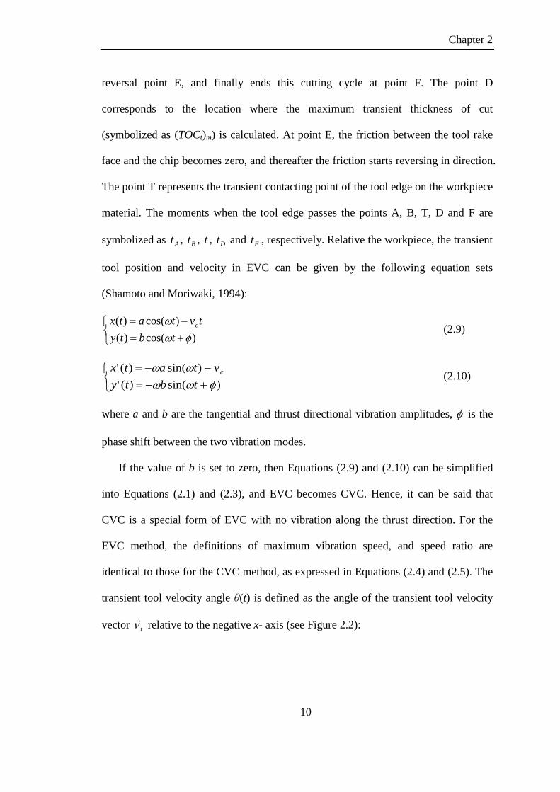
symbolized as At , Bt , t , Dt and Ft , respectively. Relative the workpiece, the transient

tool position and velocity in EVC can be given by the following equation sets

(Shamoto and Moriwaki, 1994):

+=−=

)cos()()cos()(φω

ωtbty

tvtatx c

(2.9)

+−=−−=

)sin()(')sin()('φωω

ωωtbty

vtatx c (2.10)

where a and b are the tangential and thrust directional vibration amplitudes, φ is the

phase shift between the two vibration modes.

If the value of b is set to zero, then Equations (2.9) and (2.10) can be simplified

into Equations (2.1) and (2.3), and EVC becomes CVC. Hence, it can be said that

CVC is a special form of EVC with no vibration along the thrust direction. For the

EVC method, the definitions of maximum vibration speed, and speed ratio are

identical to those for the CVC method, as expressed in Equations (2.4) and (2.5). The

transient tool velocity angle θ(t) is defined as the angle of the transient tool velocity

vector tν relative to the negative x- axis (see Figure 2.2):

Chapter 2

11

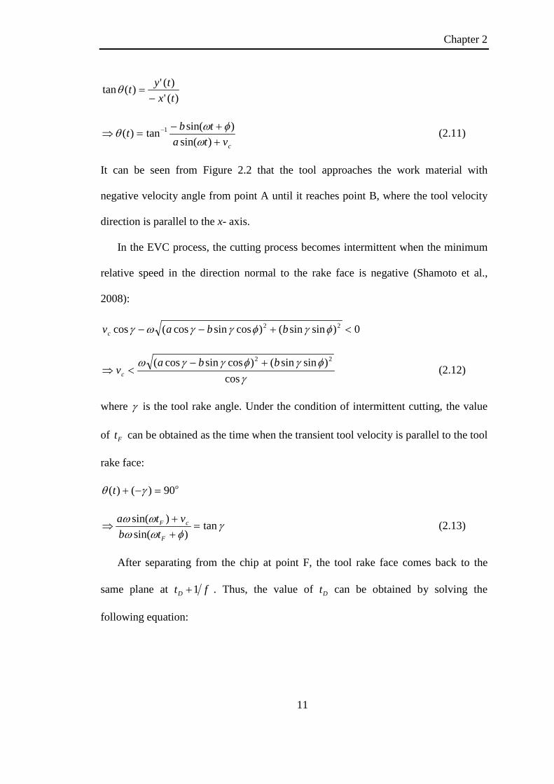
)(')(')(tantx

tyt−

=θ

cvtatbt++−

=⇒ −

)sin()sin(tan)( 1

ωφωθ (2.11)

It can be seen from Figure 2.2 that the tool approaches the work material with

negative velocity angle from point A until it reaches point B, where the tool velocity

direction is parallel to the x- axis.

In the EVC process, the cutting process becomes intermittent when the minimum

relative speed in the direction normal to the rake face is negative (Shamoto et al.,

2008):

0)sinsin()cossincos(cos 22 <+−− φγφγγωγ bbavc

γφγφγγω

cos)sinsin()cossincos( 22 bba

vc+−

<⇒ (2.12)

where γ is the tool rake angle. Under the condition of intermittent cutting, the value

of Ft can be obtained as the time when the transient tool velocity is parallel to the tool

rake face:

ot 90)()( =−+ γθ

γφωω

ωω tan)sin(

)sin(=

++

⇒F

cF

tbvta (2.13)

After separating from the chip at point F, the tool rake face comes back to the

same plane at ftD 1+ . Thus, the value of Dt can be obtained by solving the

following equation:

Chapter 2

12

γtan)()1()()1(=

−+−+

FD

FD

tyftytxftx (2.14)

If the rake angle of the cutting tool is zero (i.e. 0=γ ), which is the common case

in most EVC tests, Equations (2.12), (2.13) and (2.14) can be simplified into the

forms which are similar to Equations (2.6) (2.7) and (2.8).

Figure 2.3 illustrates the theoretical surface generation profile in the EVC process,

during which the cusps left on the finished surface perfectly reflect the vibration

marks generated by the elliptical vibration locus. The point C represents the cross-

over point, and the time when the tool edge passes this point is symbolized as Ct .

Figure 2.3. Ideal surface generation process in EVC.

According to the geometrical relationship in the EVC process, the values of At

and Ct can be determined by solving the following equation set (Shamoto and

Moriwaki, 1994):

( ) ( ) 2 /( ) ( ) 0

A C c

A C

x t x t vy t y t

π ω− = − =

-b C

x

y

B

A

Rth

T (Tb)

Tb

Tool x

a b

y

Nominal cutting direction

Chapter 2

13

cos( ) cos( ) ( ) 2 /cos( ) cos( ) 0

A C c C A c

A C

a t a t v t t vb t b t

ω ω π ωω φ ω φ

− + − =⇒ + − + =

(2.15)

The value of Bt can be obtained by solving the following equation:

bty B −=)(

0)cos( =++⇒ btb B φω (2.16)

Then, given the vibration parameters (a, b, ω and φ ) and the nominal cutting speed vc,

the theoretical roughness Rth (see Figure 2.3) along the nominal cutting direction

without considering the tool edge dimension can be calculated as follows:

( ) ( )cos( )

th A B

A

R y t y tb t bω φ

= −= + +

(2.17)

2.2 EVC systems

Based on the vibration dimension and the mechanical structure, the EVC systems

can be classified into two categories (Brehl and Dow, 2008): i) resonant EVC system

– the tool supporting structure is made to vibrate at its resonant frequency in two

dimensions, and ii) non-resonant EVC system – a mechanical linkage is used to

convert the linear expansion and contraction of piezoelectric actuator stacks into an

elliptical tool path. In the following part of this section, the resonant and non-resonant

EVC systems are reviewed.

2.2.1 Resonant EVC systems

Resonant EVC systems are the most common type of EVC systems, in which

piezoelectric actuators are used to create reciprocating harmonic motion of high-

frequency (20 kHz or above) elliptical tool motion with low amplitudes (<10 µm). A

Chapter 2

14

cutting tool is attached at the end of the vibrating horn, which is fabricated in a

delicate structure to realize desired vibration parameters. Some researchers create the

resonant EVC systems by slightly modifying the structure of resonant CVC systems,

e.g. changing the mounting position of the cutting tool (Brinksmeier and Glabe, 1999),

or mounting the tool on a specially shaped beam, instead of the original horn (Li and

Zhang, 2006). However, due to the simplicity and roughness of their design, those

EVC systems have limited advantages in terms of cutting performance compared to

CVC systems.

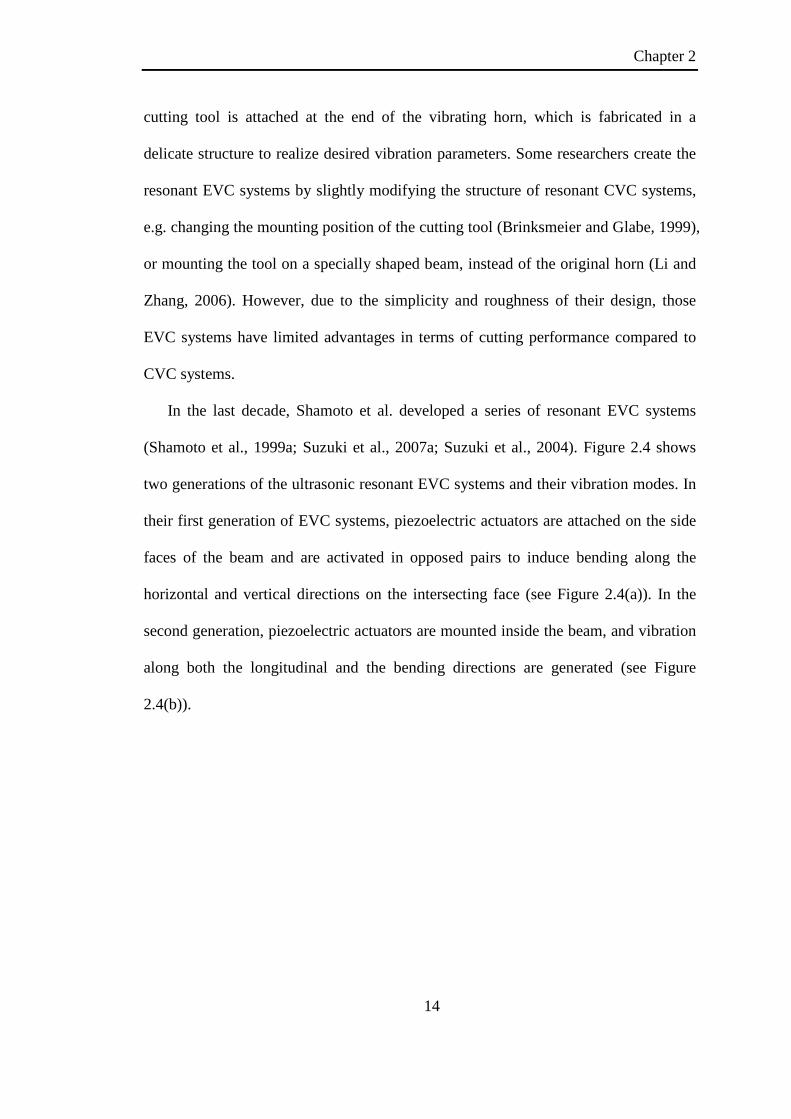
In the last decade, Shamoto et al. developed a series of resonant EVC systems

(Shamoto et al., 1999a; Suzuki et al., 2007a; Suzuki et al., 2004). Figure 2.4 shows

two generations of the ultrasonic resonant EVC systems and their vibration modes. In

their first generation of EVC systems, piezoelectric actuators are attached on the side

faces of the beam and are activated in opposed pairs to induce bending along the

horizontal and vertical directions on the intersecting face (see Figure 2.4(a)). In the

second generation, piezoelectric actuators are mounted inside the beam, and vibration

along both the longitudinal and the bending directions are generated (see Figure

2.4(b)).

Chapter 2

15

(a)

Tool position Elliptical vibration PZT actuators

5th resonant mode of bending vibration

Supporting points (nodes) 2nd resonant mode of longitudinal vibration

(b)

Figure 2.4. Two generations of ultrasonic resonant EVC systems and their vibration

modes: (a) 20 kHz (Shamoto et al., 2002), (b) 40 kHz (Suzuki et al., 2007a).

Later on, by combining the two types of ultrasonic EVC systems, Shamoto et al.

developed a new generation of 3D ultrasonic resonant EVC system. Figure 2.5 shows

the developed 3D EVC system and its vibration modes simulated by FEM software.

In order to reduce the cross talks between the longitudinal mode and the two bending

modes, a cross-talk remover was developed based on the conventional cross-talk for

the 2D EVC system (Shamoto et al., 2002).

Chapter 2

16

Figure 2.5. 3D ultrasonic resonant EVC system and its vibration modes (Suzuki et al.,

2007b).

2.2.2 Non-resonant EVC systems

Compared to resonant EVC systems, non-resonant EVC systems usually have a

relatively simpler design and a shorter development cycle, and their vibration

parameters (amplitudes, frequency and phase shift) can be adjusted in a larger range.

However, they also have a lower vibration frequency and a lower mechanical stiffness.

In non-resonant EVC systems, sinusoidal voltage signals are applied to piezoelectric

actuators, and the linear motion of the piezo stacks is converted into elliptical tool

motion by a mechanical linkage. Shamoto et al. developed the earliest non-resonant

EVC system, which has a maximum vibration frequency of 6 Hz (Shamoto and

Moriwaki, 1994). Then, Ahn et al. (1999) developed another non-resonant EVC

system based on a similar design. Figure 2.6 shows the schematic structure of the

system, where piezoelectric actuators are placed at right angles to each other and

aligned along the upfeed and vertical directions, and the flexure has an internal cross-

shaped cut-out to limit crosstalk between the two motion directions. Later on, in 2001,

a new operating design of non-resonant EVC system was developed at North Carolina

State University (Brehl and Dow, 2008). Figure 2.7 shows a schematic view of its

Chapter 2

17

operation concept. Advantages of this system are its abilities to operate over a large

range of frequencies (200~4000 Hz), tool sizes and varying orientations.

Figure 2.6. Non-resonant EVC system developed at Pusan University (Ahn et al.,

1999).

Figure 2.7. Non-resonant EVC system developed at North Carolina State University

(Brehl and Dow, 2008).

Chapter 2

18

2.3 Benefits of the EVC method

2.3.1 Smaller cutting force values

Since the CVC method is introduced, researchers have demonstrated that the

cutting force values in CVC are smaller than those measured during the CC process

for a large range of operation conditions (Astashev and Babitsky, 1998; Babitsky et

al., 2004a; Brehl and Dow, 2008; Nath and Rahman, 2008; Weber et al., 1984; Zhou

et al., 2003; Zhou et al., 2002). For the EVC method, experimental data shows that it

can provide smaller cutting force than the CVC method for the same tool geometry

and cutting conditions (Ma et al., 2004; Moriwaki and Shamoto, 1995; Nath et al.,

2009c; Shamoto et al., 1999b; Shamoto and Moriwaki, 1994, 1999). The force

reduction has been found for a large range of operating parameters and tool-

workpiece combinations in both low-frequency and ultrasonic EVC processes.

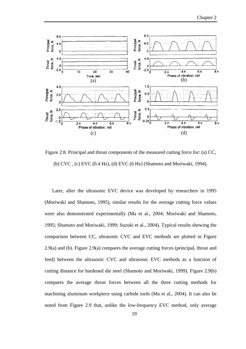
For low-frequency EVC, it was first observed experimentally in 1994 (Shamoto

and Moriwaki, 1994) that the transient cutting forces for machining oxygen free

copper are significantly reduced by applying EVC as compared with the CC and CVC

methods, as shown in Figure 2.8. From the experimental results, it can be found that

long periods of negative cutting forces exist in the EVC cycles. Such negative forces

are considered to be caused by the reversed friction force on the tool rake face.

Moreover, as the frequency is increased with the other operating parameters unvaried,

the peak cutting force decreases accordingly (see Figure 2.8(c) and (d)).

Chapter 2

19

Figure 2.8. Principal and thrust components of the measured cutting force for: (a) CC,

(b) CVC , (c) EVC (0.4 Hz), (d) EVC (6 Hz) (Shamoto and Moriwaki, 1994).

Later, after the ultrasonic EVC device was developed by researchers in 1995

(Moriwaki and Shamoto, 1995), similar results for the average cutting force values

were also demonstrated experimentally (Ma et al., 2004; Moriwaki and Shamoto,

1995; Shamoto and Moriwaki, 1999; Suzuki et al., 2004). Typical results showing the

comparison between CC, ultrasonic CVC and EVC methods are plotted in Figure

2.9(a) and (b). Figure 2.9(a) compares the average cutting forces (principal, thrust and

feed) between the ultrasonic CVC and ultrasonic EVC methods as a function of

cutting distance for hardened die steel (Shamoto and Moriwaki, 1999). Figure 2.9(b)

compares the average thrust forces between all the three cutting methods for

machining aluminum workpiece using carbide tools (Ma et al., 2004). It can also be

noted from Figure 2.9 that, unlike the low-frequency EVC method, only average

(a) (b)

(c) (d)

Chapter 2

20

cutting force can be measured by the force dynamometer for the ultrasonic EVC

process. It is because the cutting forces need to be transmitted to the piezoelectric

force sensor through intermediate elements, including VAM system itself. Such

intermediate elements work as a mass-spring-damper system with a relative low

natural frequency. Hence, the whole force measurement system acts as a low-pass

filter and can only measure the average cutting forces, instead of the high-frequency

transient cutting force.

Figure 2.9. Comparison of average cutting forces for: (a) ultrasonic CVC and

ultrasonic EVC methods (Shamoto and Moriwaki, 1999), (b) CC (“ordinary cutting”),

ultrasonic CVC and ultrasonic EVC methods (Ma et al., 2004).

2.3.2 Improved surface finish

For the CVC method, it has been known that the surface finish is better than that

obtained in the CC process for similar cutting conditions (Moriwaki et al., 1991, 1992;

Nath et al., 2007, 2008). For the EVC method, the surface finish can be further

improved compared with that achieved with the CVC and CC methods, especially in

machining difficult-to-cut materials, such as hardened steel and brittle ceramics

(b) (a)

Chapter 2

21

(Shamoto et al., 1999a; Shamoto and Moriwaki, 1999; Suzuki et al., 2007a; Suzuki et

al., 2004; Suzuki et al., 2003).

In 1999, Shamoto et al. applied ultrasonic EVC in turning of the hardened steel

using diamond tools and compared the surface roughness with that obtained with the

ultrasonic CVC method. The results plotted in Figure 2.10 show that EVC can

provide better and more sustainable surface quality than CVC. Optical quality

surfaces with maximum roughness of less than 0.05 µm can be achieved up to a

cutting distance of 2250 m with the EVC method, while the roughness obtained by the

CVC method increases rapidly at a cutting distance of about 300 m.

Figure 2.10. Comparison of surface roughness against cutting distance for CVC and

EVC (Shamoto et al., 1999a).

In 2005, Suzuki et al. have also applied the EVC method to machine brittle

materials, such as sintered tungsten carbide, zirconia ceramics, calcium fluoride and

glass. Figure 2.11 shows captured photographs for the finished surfaces of the four

brittle materials with the CC and EVC methods. It can be seen that all the comparison

results have shown that EVC performs significantly better in achieving better surface

quality than CC does. Researchers attribute such superior surface quality to the

Cutting distance, m

Surf

ace

roug

hnes

s, µm

Chapter 2

22

capability of EVC in increasing the critical depth of cut (DOC), which is an essential

parameter in machining brittle materials. Below the critical DOC, ductile-mode

machining can be achieved, and hence the smooth surface quality can be obtained,

and vice versa.

CC EVC

(a)

(b)

(c)

Chapter 2

23

(d)

Figure 2.11. Comparison of the surfaces finished by two cutting methods (CC and

EVC) for different brittle materials: (a) sintered tungsten carbide, (b) zirconia

ceramics, (c) calcium fluoride, and (d) glass (Suzuki et al., 2004).

2.3.3 Extended tool life

It has already been known that, when cutting ferrous materials with the CC

method, chemical wear rather than nonchemical abrasive wear dominates the wear of

the cutting tools made of diamond due to the iron-catalyzed graphitization of diamond

(Casstevens, 1983; Evans and Bryan, 1991; Ikawa and Tanaka, 1971; Komanduri and

Shaw, 1976; Paul et al., 1996; Shimada et al., 2004; Thornton and Wilks, 1978, 1979).

Although it is known that CVC can significantly improve the tool life compared to

CC (Nath et al., 2007; Zhou et al., 2003; Zhou et al., 2002), the EVC method can

further extend the tool life, especially when machining difficult-to-cut materials,

including hardened steel and brittle materials (Nath et al., 2009a, c; Shamoto and

Moriwaki, 1999; Suzuki et al., 2007a). By applying the EVC method, Shamoto et al.

can extend the tool life of diamond when machining steel by more than seven times

compared to the CVC method (see Figure 2.10). Figure 2.12 shows the cutting edges

Chapter 2

24

after machining hardened steel using the CVC and EVC methods. It can be seen that

the tool used in CVC is chipped, while the one used in EVC is just slightly worn

without chipping.

(a) (b)

Figure 2.12. SEM photographs of cutting edges of worn diamond tools: (a) after CVC

of steel for 1000m, and (b) after EVC of steel for 2800m (Shamoto and Moriwaki,

1999).

Not only in machining hardened steel with diamond tools, but in machining brittle

materials, the EVC method also performs well in extending the tool life. Figure 2.13

shows the comparison results of cutting performance in CC and EVC of sintered

tungsten carbide. It can be seen that the flank wear width for CC is larger than that for

EVC. Figure 2.14 shows SEM images of the cutting edges used in planing of tungsten

alloys with the CC and EVC methods. Considerable rake and flank wear and adhesion

of machined material can be observed for the tool used in CC, while there is no tool

wear or adhesion for EVC.

Chapter 2

25

Figure 2.13. Comparison of cutting performance between the CC and EVC methods

(Nath et al., 2009c).

(a) (b)

Figure 2.14. Cutting edges of diamond tools used for planing tungsten alloys with: (a)

after CC of 1.08 m, and (b) after EVC of 1.35 m (Suzuki et al., 2007a).

2.3.4 Improved form accuracy and burr suppression

Ma et al. investigated the form accuracy in CC, CVC and EVC and compared the

experimental results, as shown in Figure 2.15 (Ma et al., 2004). It can be observed

that the shape error is reduced by 79% from 28 µm to 6 µm using the CVC method,

while the EVC method can improve the form accuracy by about 98% compared to the

1) Cutting force (N), 2) Flank wear width (µm) x10, 3) Ra (µm) x10, and 4) Rz (µm) x10.

EVC CC

Chapter 2

26

CC method. Furthermore, Ma et al. have also experimentally and theoretically proved

that regenerative chatter occurring in ordinary cutting process can be suppressed

effectively by adding elliptical vibration on the cutting tool (Ma et al., 2011). The

authors attribute this fact to the separating characteristic and the characteristic of

reversed frictional direction between the tool rake face and the chip.

Figure 2.15. Influence of the three cutting methods (CC, CVC and EVC) on the shape

error (Ma et al., 2004).

In 2005, Ma et al. have also investigated the suppression of burrs in EVC of

aluminum (52S). Figure 2.16 shows heights of the feed-direction burrs measured in

the CC, CVC and EVC processes. Compared to CC and CVC, the height of burrs in

EVC can be reduced significantly. Such fact is considered to be caused by the reduced

average pushing stress and the reduced average bending stress of deformation zone on

the workpiece edge in burr formation.

Measured position from end, mm

Prof

iles o

f fin

ishe

d su

rfac

es, µ

m

Chapter 2

27

Figure 2.16. Height of burrs for the CC, CVC and EVC methods (Ma et al., 2005).

2.4 Analytical studies of EVC

2.4.1 Force models

In order to investigate the reason for the smaller cutting forces obtained by the

EVC method, Shamoto et al. developed the first generation of force model in 1999

(Shamoto et al., 1999b), in which an average friction angle β defined in the EVC

process is calculated based on the kinetic-friction angle β . Then the average shear

plane angle φ can be obtained by applying the famous maximum shear stress

principle (Lee and Shaffer, 1951). However, the transient cutting force in EVC was

not predicted by the authors in their study.

Later on, in 2008, Shamoto et al. developed a 3D analytical EVC force model, in

which they attributed the thrust force reversal to the friction force reversal on the tool

rake face (Shamoto et al., 2008). Moreover, they explained that, during each EVC

cycle, the friction force reverses at the position where the speed component of

transient tool velocity along the tool rake face exceeds the real chip velocity (point E

1/Rs

Hei

ght o

f bur

rs, µ

m

Chapter 2

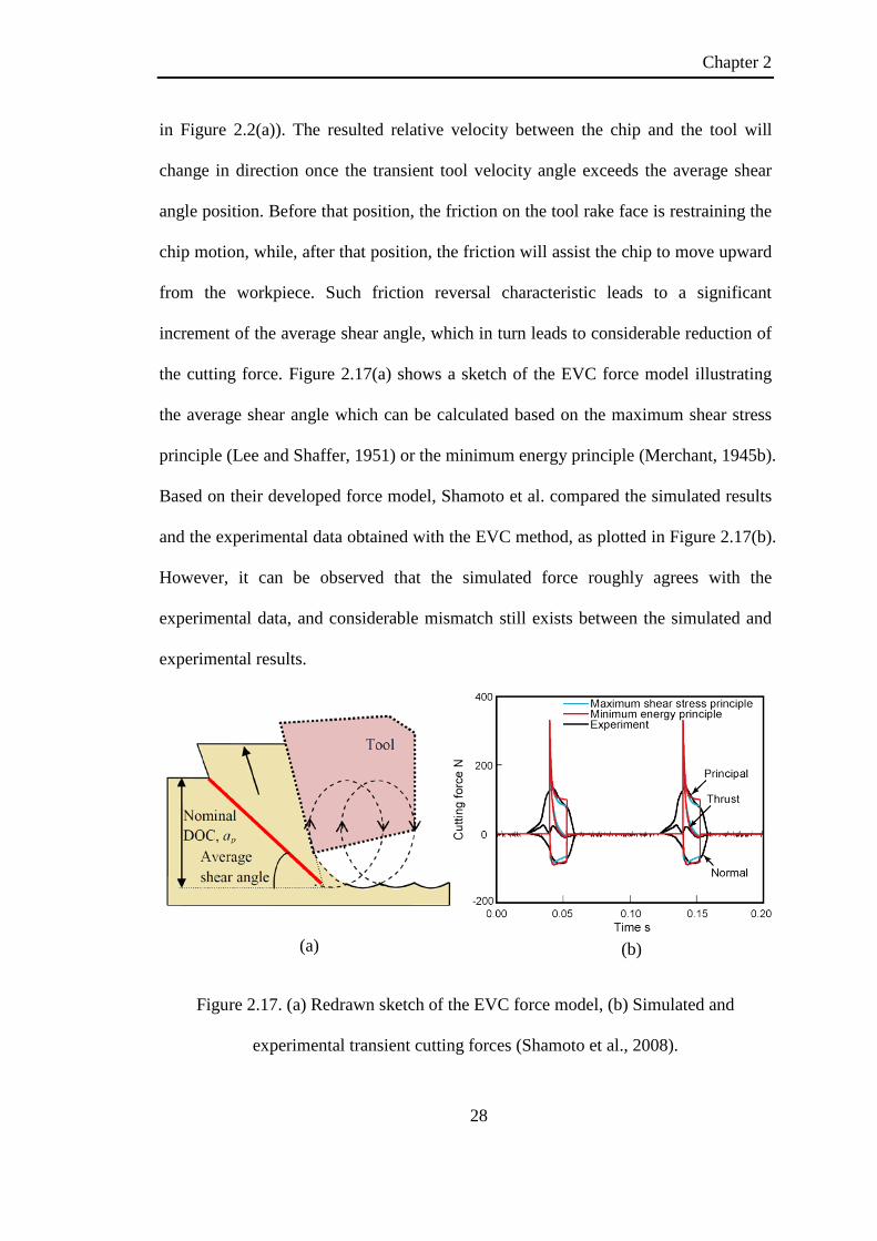
28

in Figure 2.2(a)). The resulted relative velocity between the chip and the tool will

change in direction once the transient tool velocity angle exceeds the average shear

angle position. Before that position, the friction on the tool rake face is restraining the

chip motion, while, after that position, the friction will assist the chip to move upward

from the workpiece. Such friction reversal characteristic leads to a significant

increment of the average shear angle, which in turn leads to considerable reduction of

the cutting force. Figure 2.17(a) shows a sketch of the EVC force model illustrating

the average shear angle which can be calculated based on the maximum shear stress

principle (Lee and Shaffer, 1951) or the minimum energy principle (Merchant, 1945b).

Based on their developed force model, Shamoto et al. compared the simulated results

and the experimental data obtained with the EVC method, as plotted in Figure 2.17(b).

However, it can be observed that the simulated force roughly agrees with the

experimental data, and considerable mismatch still exists between the simulated and

experimental results.

Figure 2.17. (a) Redrawn sketch of the EVC force model, (b) Simulated and

experimental transient cutting forces (Shamoto et al., 2008).

(a) (b)

Chapter 2

29

2.4.2 Surface generation and critical speed ratio

Shamoto et al., based on their proposed purely geometrical model for EVC process

(Shamoto and Moriwaki, 1994), developed a calculation method for the height of the

generated cusps, and also investigated the effects of vibration frequency on the

surface generation. The theoretical surface generation profile without considering the

tool edge radius is shown in Figure 2.3, where the cusps left on the finished surface

perfectly reflect the vibration marks generated by the elliptical vibration locus.

For ductile machining of hard and brittle materials, the DOC should be selected

carefully to make its value lower than the critical DOC, which is extremely low (1 µm

or less) for common brittle materials such as sintered tungsten carbide, glass and

ceramics (Liu et al., 2004; Liu and Li, 2001). In order to maintain the ductile-mode

machining in EVC of brittle materials, Nath et al. obtained a critical speed ratio of

0.12837 based on an analytical investigation of the geometrical EVC process (Nath,

2008). Figure 2.18 shows the Nomraski photographs of machined surfaces of sintered

tungsten carbide at different speed ratios, which are smaller or larger than the critical

speed ratio. It can be seen that, below the critical value of 0.12837, ductile-mode

machining of the brittle materials can be obtained, which is considered by Nath et al.

to be caused by a reduced maximum thickness of cut under such condition.

Chapter 2

30

(a)

(b)

Figure 2.18. Photographs of the machined surfaces of sintered tungsten carbide for

different values of speed ratios: (a) 0.075 (Rs < 0.12837), (b) 0.131 (Rs > 0.12837) (Nath

et al., 2011).

2.4.3 FEM and MD analysis

For the CVC process, Babitsky et al. conducted a series of finite element method

(FEM) studies on its cutting mechanics and studied the chip deformation and stress

distribution in detail (Ahmed et al., 2006, 2007a, b; Babitsky et al., 2004b;

Mitrofanov et al., 2005a; Mitrofanov et al., 2004, 2005b). For the EVC process, very

few FEM studies have been conducted on its unique cutting mechanism. Amini et al.

simulated the EVC process using FEM software and compared the results with those

of CC and CVC in their study (Amini et al., 2010). Deformation and stress

distribution of the workpiece material and the cutting mechanics are analyzed and

discussed for the three cutting methods. Figure 2.19 shows the chip formation and

Chapter 2

31

stress distribution in the EVC process for one cutting cycle. Their simulation results

indicate that the initial contacting part in EVC (point A to point D in Figure 2.2(a)) is

not formed into a chip but pushed into the workpiece. Such process leads to an

extremely high equivalent Von Mises stress at this stage, as shown in Figure 2.19(c).

Amini et al. have also compared simulated cutting force values with the experimental

ones obtained by Shamoto et al. (1994), and they are found in a good agreement with

each other.

Figure 2.19. Chip formation and stress distribution simulated in one vibration cycle in

EVC (Amini et al., 2010).

Chapter 2

32

Liang et al. studied the nano-metric behavior of EVC of single crystal silicon with

SCD tools by employing molecular dynamics (MD) analysis (2006). The cutting force

and stress distribution in the EVC process have been analyzed. Unfortunately, no

experimental studies have been conducted in their study, and the given vibration

parameters (amplitudes and frequency) in the simulation are either too small or too

large.

2.5 Concluding remarks

As mentioned above, although extensive experimental research has been

conducted on the average cutting force in EVC, very few studies have been found on

the transient cutting force, which is strongly correlated with the inherent cutting

mechanism of the EVC process. Researchers studied the transient cutting force in

EVC at different frequencies, and proposed a simple analytical force model for the

transient cutting force. However, besides the frequency, the effects of other cutting

and vibration conditions on the transient cutting force have not been studied yet.

Moreover, the predicted cutting force based on the existing proposed model does not

match well with the experimental one, which might be caused by the overlook of

some transient characteristics, such as transient thickness of cut, transient shear angle,

and the reversal of friction direction.

Shamoto et al. developed a calculation method for the height of the generated

vibration cusps along the nominal cutting direction, which will eventually increase the

roughness of machined surface and are considered detrimental for achieving high-

quality mirror surface. Such drawback of the EVC method may become an important

reason which can limit its wider application. However, until now, very little research

has been conducted to study the effects of machining parameters on the surface

Chapter 2

33

generation. Moreover, in the proposed calculation model, a critical assumption is that

the tool edge is assumed to be perfectly sharp, which may not be reasonable for the

situation when the edge radius of non-SCD tools is comparable to the vibration

amplitudes.

Although researchers have used SCD tools to machine hardened steel with the

EVC method, and observed significantly longer tool life compared to the CC and

CVC methods, the application feasibility of inexpensive PCD tools, instead of SCD

tools, under the EVC method to obtain mirror quality surface on hardened steel for die

and mold applications has not been justified yet. Moreover, the reason claimed by

most previous researchers for the reduced diamond tool wear in VAM of steel was

found to be ambiguous and not reasonable, and its correctness has not been confirmed

experimentally and theoretically.

Chapter 3

34

Chapter 3: Experimental investigation of

transient cutting force in EVC

Cutting force is considered as the most important indicator of machining state and

quality. Analysis of the cutting force plays an important role in the determination of

characteristics of machining performances like tool wear, surface quality, cutting

energy, and machining accuracy. As mentioned in Chapter 2, in order to investigate

the fundamental cutting mechanics of the EVC process, researchers (Shamoto and

Moriwaki, 1994) have studied the transient cutting force at different vibration

frequencies, and found that higher vibration frequency can reduce the transient cutting

force. However, besides the vibration frequency, the effects of other cutting and

vibration conditions (including tangential amplitude, thrust amplitude and speed ratio)

on the transient cutting force have not been studied yet.

Speed ratio is considered as one of the most essential parameters in the EVC

method (Nath et al., 2011; Shamoto et al., 2008). It was found that the speed ratio has

significant effects on cutting performances (e.g. time-averaged cutting force, tool

wear and surface roughness). Tangential and thrust amplitudes are two key parameters

in vibration-assisted machining technology (Brehl and Dow, 2008). Tangential

amplitude is used to discriminate the CVC method from the CC method, and thrust

amplitude is used to discriminate the EVC method and the CVC method. For the EVC

method, both the tangential and thrust amplitudes are larger than zero, and the tool tip

vibrates in two dimension, whereas in the CVC method, the thrust amplitude is equal

Chapter 3

35

to zero, and the tool tip vibrates in only one dimension, while for the CC method, both

the tangential and thrust amplitudes are equal to zero, and the tool tip does not vibrate.

Unfortunately, the above three essential parameters’ effects (speed ratio, tangential

and thrust amplitudes) on the transient cutting force in the EVC process have not been

studied yet. Therefore, an intensive experimental investigation to study their effects is

necessary to enhance the understanding of fundamental material removal mechanism

in the EVC process and to explain and predict the cutting performance under various

cutting and vibration conditions.

In this chapter, the characteristics of the EVC process are investigated analytically

by studying the transient thickness of cut (TOCt) and the friction reversal process in

each EVC cycle. Then, a series of low-frequency orthogonal EVC tests are conducted

to study the effects of three essential parameters on the transient cutting force. By

analyzing the values of TOCt and the friction reversal time for each EVC test, results

of the transient cutting force at different conditions are interpreted analytically.

3.1 Characteristics of the EVC process

3.1.1 Transient thickness of cut

It is understood the variation of transient TOC (TOCt) is a key characteristic in the

EVC process (Nath et al., 2011). Figure 3.1(a) and (b) show the 2D view of the EVC

process before and after the tool edge passes the maximum TOCt (symbolized as

(TOCt)m) point D, respectively. The value of TOCt gets continuously varied and is

always smaller than the nominal depth of cut ap due to the overlapping cutting cycles.

During each EVC cycle, the tool edge starts cutting from point A on the machined

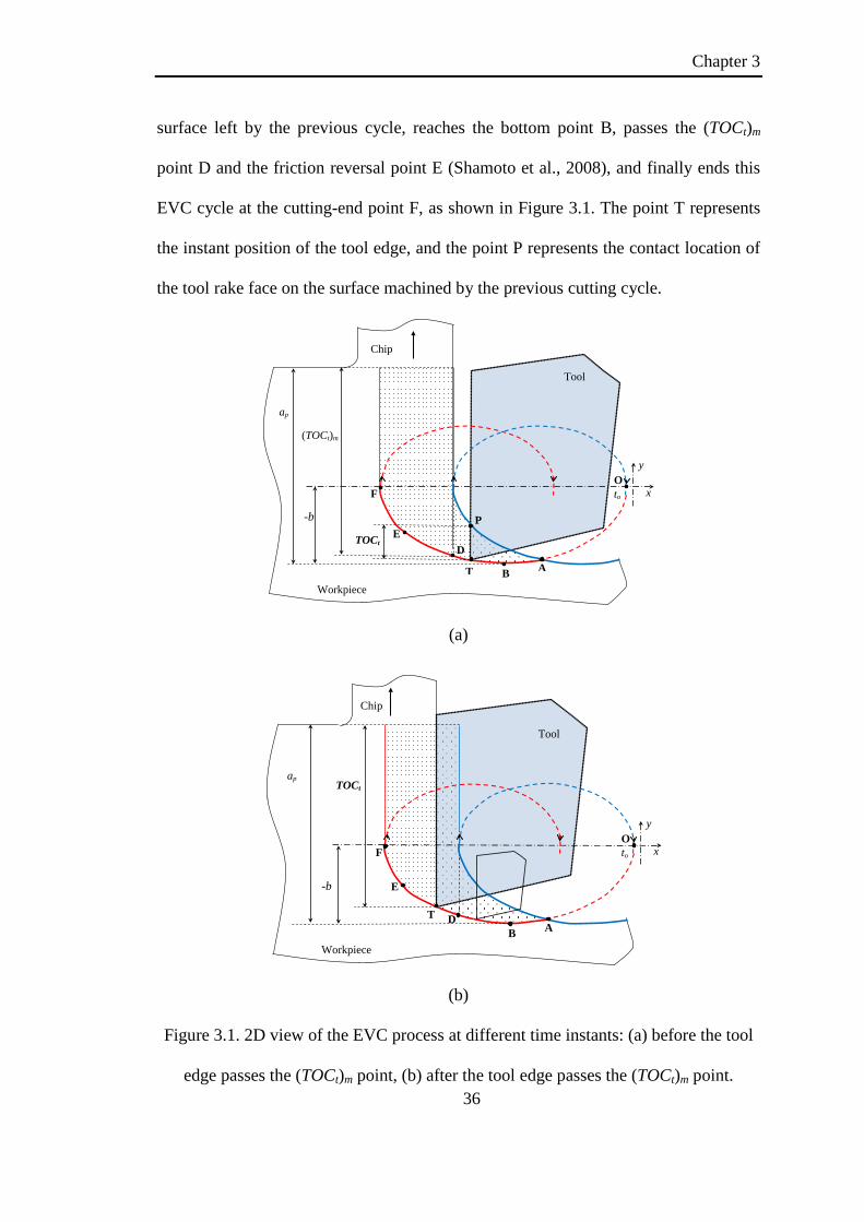
Chapter 3

36

surface left by the previous cycle, reaches the bottom point B, passes the (TOCt)m

point D and the friction reversal point E (Shamoto et al., 2008), and finally ends this

EVC cycle at the cutting-end point F, as shown in Figure 3.1. The point T represents

the instant position of the tool edge, and the point P represents the contact location of

the tool rake face on the surface machined by the previous cutting cycle.

A

F

Chip

Tool

Workpiece B

O

TOCt

(TOCt)m

ap

x to

D

-b

y

P

T

E

(a)

A

F

Chip

Tool

Workpiece B

O

TOCt ap

x to

D

-b

y

E

T

(b)

Figure 3.1. 2D view of the EVC process at different time instants: (a) before the tool

edge passes the (TOCt)m point, (b) after the tool edge passes the (TOCt)m point.

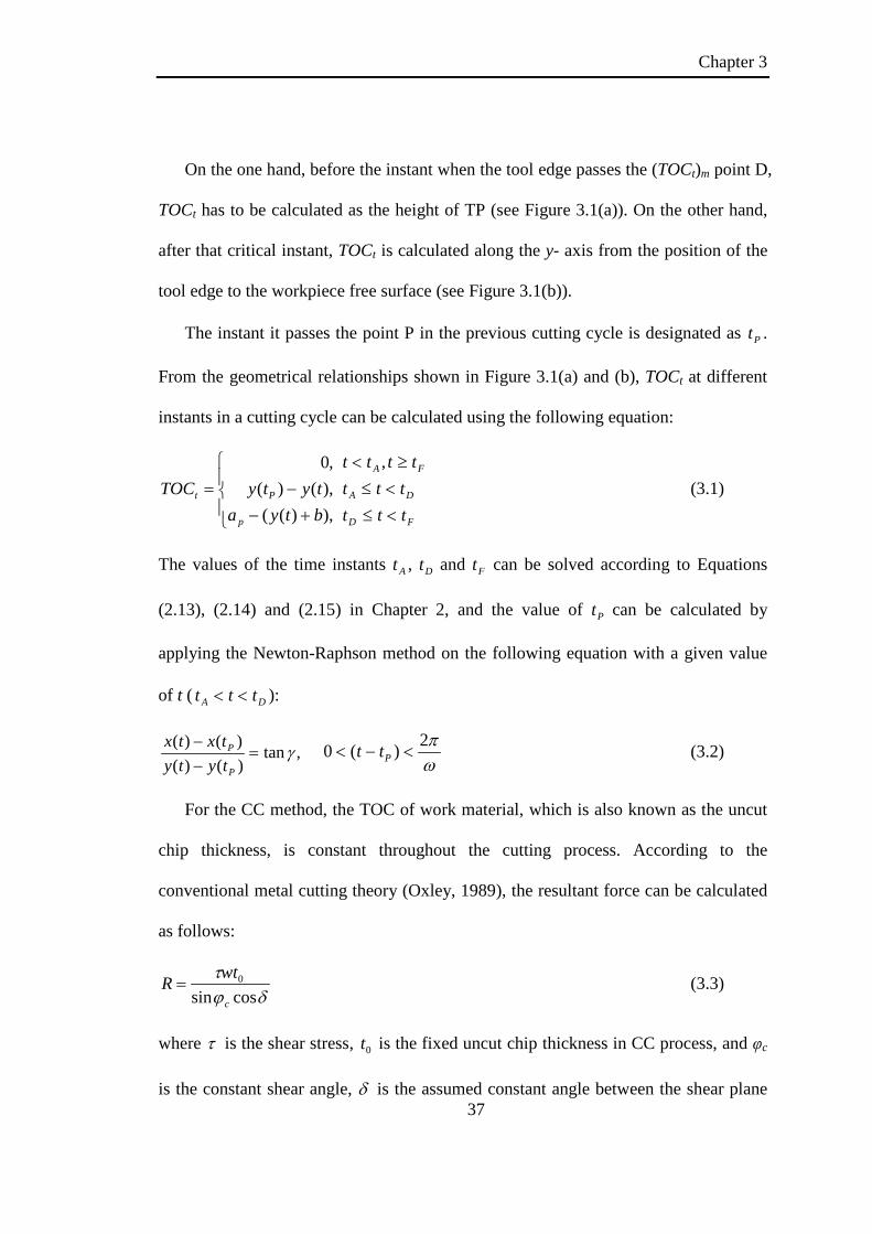
Chapter 3

37

On the one hand, before the instant when the tool edge passes the (TOCt)m point D,

TOCt has to be calculated as the height of TP (see Figure 3.1(a)). On the other hand,

after that critical instant, TOCt is calculated along the y- axis from the position of the

tool edge to the workpiece free surface (see Figure 3.1(b)).

The instant it passes the point P in the previous cutting cycle is designated as Pt .

From the geometrical relationships shown in Figure 3.1(a) and (b), TOCt at different

instants in a cutting cycle can be calculated using the following equation:

+−−=

),)((),()(,0

btyatytyTOC

p

Pt

FD

DA

FA

tttttt

tttt

<≤<≤≥< ,

(3.1)

The values of the time instants At , Dt and Ft can be solved according to Equations

(2.13), (2.14) and (2.15) in Chapter 2, and the value of Pt can be calculated by

applying the Newton-Raphson method on the following equation with a given value

of t ( DA ttt << ):

,tan)()()()(

γ=−−

P

P

tytytxtx

ωπ2)(0 <−< Ptt (3.2)

For the CC method, the TOC of work material, which is also known as the uncut

chip thickness, is constant throughout the cutting process. According to the

conventional metal cutting theory (Oxley, 1989), the resultant force can be calculated

as follows:

δϕτ

cossin0

c

wtR = (3.3)

where τ is the shear stress, 0t is the fixed uncut chip thickness in CC process, and φc

is the constant shear angle, δ is the assumed constant angle between the shear plane

Chapter 3

38

and the resultant force, as shown in Figure 3.2. It can be seen that the value of R is in

direct proportion to 0t :

0tR ∝ (3.4)

Although the EVC process is different from the CC process in the material

removal process, the fundamental cutting mechanism should be the same, and hence

the thin shear plane theory will still be applicable to the EVC process. Therefore,

keeping the other parameters (e.g. shear angle, shear stress, etc) unvaried, the

transient resultant cutting force R(t) applied on the cutting tool should be in direct

proportion to the value of TOCt in the EVC process:

tTOCtR ∝)( (3.5)

3.1.2 Friction reversal process in the EVC process

For the CC method, a schematic illustration of the CC process is shown in Figure

3.2, where the symbols, R, Fns, Fn, Fp and Ft represent the resultant force, the normal

force perpendicular to the shear direction, the normal force perpendicular to the rake

face, the principal force along the nominal cutting direction, and the thrust force

perpendicular to the nominal cutting direction, respectively. βk represents the kinetic-

friction angle between the tool rake face and the work material. sv , tv and ctv

represent the transient shear velocity, the transient tool velocity relative to the

workpiece, and the transient chip velocity relative to the tool. It can be seen from

Figure 3.2 that the tool velocity tv always stays invariant in direction, the shear

velocity sv and the chip velocity ctv also remain constant in direction. Due to the

sliding movement of the chip on the tool rake face throughout the CC process, kinetic

friction is induced and tends to push the chip material down toward the workpiece.

Chapter 3

39

γ

S

O cϕ

Tool

Fp Ft

R Fns δ Fs

Ff Fn

R kβ

Chip

Workpiece

γβ −k

tv

ctv sv

δ t0

Figure 3.2. Schematic illustration of the CC process.

By analyzing the recorded data of the transient cutting force in the EVC process,

researchers have proven the existence of friction force with reversed direction

(Shamoto and Moriwaki, 1994). Such friction reversal process is considered to be

another essential characteristic of the EVC method, besides the variation of TOCt.

Later on, researchers (Shamoto et al., 2008) proposed that there exists a critical

friction reversal point E (see Figure 3.1), at which the friction on the tool rake face is

about to reverse in direction, meaning that the friction force is zero at this critical

point.

Before the tool edge passes the point E (i.e. Ett < , Et represents the time when

the tool edge passes point E), the tool is pushing the chip downward to the workpiece,

which is similar to the CC process (see Figure 3.2). After the tool edge has passed this

critical friction reversal point E in the EVC process (i.e. Ett > ), the tool will pull the

chip upward from the workpiece. Figure 3.3 shows the force and velocity

relationships at an instant where the friction is reversed in direction.

Chapter 3

40

E

Tool

tϕ

γ

tv ctv

sv

S′

kβ

R Ff

Fn

δ Fs

Fns

R

Fp Ft

Figure 3.3. Force and velocity relationships after the tool passes the friction reversal

point in the EVC process.

In order to clearly analyze the transient friction angle and the transient shear angle,

a schematic illustration of the transient friction angle and the induced transient shear

angle in an EVC cycle is drawn in Figure 3.4(a) and (b). The negative value of the

kinetic-friction angle -βk is used to represent the reversed friction in direction, and the

kinetic-friction angle is assumed to be constant throughout the cutting process. The

points E1 and E2 in Figure 3.4 represent two friction reversal points, and 1Et and 2Et

represent the corresponding friction time instants ( 21 EE tt < ). Once the friction force

is reversed in direction, the pulling motion away from the workpiece after the point E

will lead to an increased transient shear angle, as shown in Figure 3.4(b). kcϕ and

krϕ are used to represent the transient shear angles before and after the tool edge

passes the friction reversal point ( krkc ϕϕ < ), and the value of kcϕ and krϕ are

assumed to be constant in the EVC process.

Chapter 3

41

0 π/2 π

0

Phase of vibration, rad

Tran

sien

t fric

tion

angl

e

3π/2

kβ

kβ−

ωtA ωtF

A

E2

F

ωtE2

E1

ωtE1

(a)

0 π/2 π


Tran

sien

t she

ar a

ngle

3π/2

krϕ

kcϕ

ωtA ωtF

A

E2

F

ωtE2

E1

ωtE1 0

(b)

Figure 3.4. Schematic illustration of (a) transient kinetic-friction angle, and (b)

transient shear angle in an EVC cycle.

Therefore, according to Figure 3.4, it can be predicted that, the smaller the value

of Et , the earlier the friction starts reversing, the earlier transient shear angle starts

increasing, and hence the larger portion ( FE tt ~ ) of the increased shear angle krϕ .

Considering the inverse proportion relationship between the resultant force and the

shear angle (see Equation (3.3)), it is reasonable to derive the following relationship

between the friction reversal time and the transient resultant force:

↓→↓ )(tRtE (3.6)

Chapter 3

42

3.2 Experimental details

As mentioned in Chapter 2, it is known that researchers usually apply high-

frequency vibration (at ultrasonic level of about 20 kHz or more) to enhance the

productivity and cutting performances in practical metal cutting with the EVC method

(Nath et al., 2009a; Shamoto and Moriwaki, 1999). However, it is impossible to

measure the transient force values with ultrasonic frequency using the state-of-the-art

measurement technology, due to the low natural frequency (about 5 kHz or less) of

common dynamometers. It is because the measurement system may act as a low pass

filter (Brehl and Dow, 2008), which is only able to measure the filtered time-averaged

cutting force, but not the original transient force. Therefore, in order to study the

transient cutting force in the EVC process, it is necessary to employ a low-frequency

EVC method, instead of the ultrasonic EVC method.

The low-frequency elliptical vibration motion of the cutting tool relative to the

workpiece is generated by a combined movement of the X- and Y- axes of a CNC

ultraprecision machine tool (Toshiba ULG-100H3). The machine tool has a 10 nm

linear resolution along the X-, Y- and Z- axes, which makes it reasonable to

accurately drive the low-frequency EVC motion. In order to generate the elliptical

vibration motion of tool tip, first, some ideal elliptical vibration loci are created by

employing Equation (2.9) with preset cutting and vibration conditions. Then, the

elliptical loci are fitted by sampling 360 points for each cutting cycle (i.e. every 2π

phase), and G-codes are generated based on coordinates of the derived points. Figure

3.5 shows the schematic procedures for generating the low-frequency EVC motion.

Chapter 3

43

Tool

Sampling and G-code generation

Ultraprecision CNC machine G90G01

X0.02Y-0.003F200.0

X0.01998Y-0.00309F0.48

......

......

G Code

Axis control

EVC locus

Y

X

Figure 3.5. Illustration of the procedures for generating the low-frequency EVC

motion.

In this study, a series of orthogonal EVC tests are conducted on 6061 aluminum

alloy workpiece. Figure 3.6 shows a schematic illustration of the experimental setup

for the cutting tests. The force signals are measured by a 3-component mini-

dynamometer with 1 mN resolution mounted on the tool post and recorded with a

real-time digitized recorder. In order to avoid the effect of tool edge geometry in this

orthogonal EVC test, a flat-nose SCD tool is used, with 0o rake angle and 7o flank

angle. Figure 3.7 shows a microscope photograph of the flat nose diamond tool, which

has a 760 µm nose width. Its tool edge radius is measured to be about 0.15 µm by

applying an indentation method proposed by previous researchers (Li et al., 2003).

Chapter 3

44

Figure 3.6. Illustration of the experimental set-up for the low-frequency EVC tests.

760 μm

7o

Front view Section view

Cutting edge

Rake face Flank face Section view

Side view

500 μm

Figure 3.7. Microscope photograph (X50) of the flat nose diamond tool.

Chapter 3

45

Table 3.1 shows the cutting and vibration conditions for the orthogonal EVC tests.

The speed ratio in this table is changed by varying the value of vc. Four different

speed ratios, five principal amplitudes and five thrust amplitudes were selected to

study their effects on the transient cutting force, while keeping the other cutting and

vibration conditions unvaried. Figure 3.8 shows the experimental set-up for the

cutting tests.

Table 3.1. Cutting and vibration conditions of the orthogonal EVC tests.

Tool Flat nose diamond tool Workpiece 6061 aluminum alloy Width of cut, w [µm] 400 Nominal uncut chip thickness, ap [µm] 15 Lubrication condition Dry cutting Vibration frequency, f [Hz] 0.25 Phase shift, φ [deg] 90 Speed ratio, Rs (Nominal cutting speed, vc [mm/min])

0.025 (0.047)

0.05 (0.094)

0.075 (0.141)

0.1 (0.188)

Tangential amplitude, a [µm] 8 11 14 17 20 Thrust amplitude, b [µm] 2 5 8 11 14

Vacuum chuck

Workpiece

Flat-nose diamond tool

Force dynamometer

Fixture

Figure 3.8. Experimental set-up for the orthogonal EVC tests.

Chapter 3

46

3.3 Results and analysis

In this section, results of the transient cutting force at different speed ratios,

tangential and thrust amplitudes are presented, and then the results are carefully

analyzed and explained by comparing the values of TOCt and friction reversal time

for the specific cutting and vibration conditions.

3.3.1 Effect of speed ratio

Figure 3.9(a) shows the recorded experimental values of the transient force

components (the principal and thrust force) in an EVC cycle at two speed ratios

(0.025 and 0.1) with 20 µm tangential amplitude and 5 µm thrust amplitude. Figure

3.9(b) shows the values of the maximum resultant force Rmax against different speed

ratios.

From Figure 3.9(a), it can be seen that the transient principal force starts

increasing from zero, reaches the maximum value at some point, then decreases

slightly, and finally drops to zero after the disengagement of tool and chip. The

transient thrust force starts from zero and increases gradually, which is similar to the

trend of transient principal force in the beginning portion. However, after reaching its

maximum positive value, it starts decreasing and becomes negative. Then, as time

goes on, the thrust force remains negative in the following portion of the EVC cycle

until the tool is fully disengaged with the formed chip. It means that the thrust force is

reversed in direction, and such reversal process is considered to be caused by the

reversed direction of friction between the tool rake face and the formed chip,

indicating that the tool is pulling the chip upward from the workpiece. From Figure

3.9(b) It can be observed that the value of Rmax increases gradually with the increment

Chapter 3

47

of Rs. The value of Rmax is increased by more than 45% when the speed ratio is

increased from 0.025 to 0.1.

0 π/2 π 3π/2 2π-1

0

1

2

3

4

5

Phase angle, rad

Cut

ting

forc

e, N

Rs=0.1Rs=0.025

Principal force

Thrust force

0

1

2

3

4

5

6

0.025 0.05 0.075 0.1

Max

imum

resu

ltant

forc

e, R

max

, (N

)

Speed ratio, Rs

(a) (b)

Figure 3.9. The effect of speed ratio on (a) the transient cutting force components, (b)

the maximum resultant cutting force.

In order to find the inherent reasons for the effects of speed ratio on transient

cutting force, the values of TOCt and (TOCt)m against different speed ratios are

calculated using Equation (3.1), as presented in Figure 3.10(a) and (b). The cutting

and vibration conditions of Figure 3.10 are same with those of Figure 3.9. It can be

observed that both the values of TOCt and (TOCt)m increase with the increment of the

speed ratio, similar to the phenomenon shown in Figure 3.9. Considering the direct

proportion relationship between TOCt and the transient cutting force (see Equation

(3.5)), the variation of TOCt can be treated as a major reason for the variation

tendency found in Figure 3.9.

Chapter 3

48

0 π π/2 3π/2 2π0

5

10

15

20


TOC

t, μm

Rs=0.1Rs=0.025

ap

0

3

6

9

12

15

0.025 0.05 0.075 0.1

(TO

Ct) m

, µm

Speed ratio, Rs

(a) (b)

Figure 3.10. The effect of speed ratio on the values of (a) TOCt, (b) (TOCt)m.

As the tool rake angle is zero in the cutting tests, it can be derived that the

transient friction force should be equal to the transient thrust force. Hence, the friction

reversal time Et can be calculated as the time when the thrust force is about to

become negative. Figure 3.11 shows the values of Et at different speed ratios. It can

be seen that the value of Et increases slightly with the increment of Rs, but the effect

of speed ratio on the value of Et is not significant. Hence, considering the direct

proportion relationship between the transient cutting force and Et (see Equation (3.6)),

it can be concluded that the variation of friction reversal time may contribute as a

minor reason for the variation tendency observed in Figure 3.9.

Chapter 3

49

0

0.5

1

1.5

2

0.025 0.05 0.075 0.1

Fric

tion

reve

rsio

n tim

e, t E

, (s)

Speed ratio, Rs

Figure 3.11. The effect of speed ratio on the value of friction reversal time.

3.3.2 Effect of tangential amplitude

In order to investigate the effect of tangential amplitude, the speed ratio is kept

constant at 0.1 by changing the value of vc accordingly, and the thrust amplitude is

kept constant at 5 µm. Figure 3.12(a) and (b) show the effect of different tangential

amplitudes on the transient cutting force and Rmax. It can be seen from Figure 3.12 that

the value of transient cutting force increases gradually with the increment of

tangential amplitude, and the value of Rmax is increased by 35% when the tangential

amplitude is increased from 8 to 20.

Chapter 3

50

0 π/2 π 3π/2 2π-1

0

1

2

3

4

5

Phrase angle, rad

Cut

ting

forc

e, N

a =20 µma =8 µm

Principal force

Thrust force

0

1

2

3

4

5

6

8 11 14 17 20Max

imum

resu

ltant

forc

e, R

max

, (N

)

Tangential amplitude, a, (µm)

(a) (b)

Figure 3.12. The effect of tangential amplitude on (a) the transient cutting force

components, (b) the maximum resultant cutting force.

Figure 3.13(a) and (b) show the value of TOCt and (TOCt)m at different tangential

amplitudes. It can be observed from Figure 3.13(a) that the value of TOCt is identical

at different tangential amplitudes. Accordingly, the value of (TOCt)m does not change

against the tangential amplitude. Hence, it can be concluded that the variation of TOCt

is not a reason for the variation tendency found in Figure 3.12. Figure 3.13(c) shows

that the value of Et increases gradually with the increment of tangential amplitude.

Considering the direct proportion relationship between Et and the transient cutting

force described in the above section, it is reasonable to derive that the increment of

transient cutting force with the increment of tangential amplitude is caused by the

increment of the friction reversal time. The larger value of Et will postpone the

occurrence of friction reversal, and hence reduce the portion of increased transient

shear angle in the EVC process.

Chapter 3

51

0 π/2 π 3π/2 2π0

5

10

15

20


TOC

t, µm

ap

a =8, 20 μm

0

3

6

9

12

15

8 11 14 17 20

(TO

Ct) m

, µm


(a) (b)

0

0.5

1

1.5

2

8 11 14 17 20

Fric

tion

reve

rsio

n tim

e, t E

, (s)


(c)

Figure 3.13. The effect of tangential amplitude on the values of (a) TOCt, (b) (TOCt)m,

(c) friction reversal time.

3.3.3 Effect of thrust amplitude

Figure 3.14(a) and (b) show the effect of different thrust amplitudes on the

transient cutting force and Rmax with 20 µm tangential amplitude and 0.1 speed ratio.

Unlike the case for the tangential amplitude, it can be observed that the value of Rmax

decreases with the increment of thrust amplitude, and the value of Rmax is decreased

by about 40% when the thrust amplitude is increased from 2 to 14.

Chapter 3

52

0 π/2 π 3π/2 2π-1

0

1

2

3

4

5

6

Phase angle, rad

Cut

ting

forc

e, N

b =14 µmb = 2 µm

Principal force

Thrust force

0

1

2

3

4

5

6

2 5 8 11 14Max

imum

resu

ltant

forc

e, R

max

, (N

)

Thrust amplitude, b, (µm)

(a) (b)

Figure 3.14. The effect of thrust amplitude on (a) the transient cutting force

components, (b) the maximum resultant cutting force.

Figure 3.15(a) and (b) show the values of TOCt, (TOCt)m and Et at different thrust

amplitudes. It can be seen that TOCt and (TOCt)m gradually decreases with the

increment of thrust amplitude. Figure 3.15(c) shows that the value of Et also

decreases with the increment of thrust amplitude. Considering the direct proportion

relationship between the transient cutting force and the values of both TOCt and Et , it

can be concluded that the decrement of TOCt and Et contribute as two major reasons

for the variation tendency of transient cutting force.

Chapter 3

53

0 π/2 π 3π/2 2π0

5

10

15

20


TOC

t, μm

b =14 μmb =2 μm

ap

0

3

6

9

12

15

2 5 8 11 14

(TO

Ct) m

, µm

Thrust amplitude, b, µm

(a) (b)

0

0.5

1

1.5

2

2 5 8 11 14

Fric

tion

reve

rsio

n tim

e, t E

, (s)

Thrust amplitude, b, (µm)

(c)

Figure 3.15. The effects of thrust amplitude in the EVC process on the values of (a)

TOCt, (b) (TOCt)m, (c) friction reversal time.


In this chapter, the effects of three essential cutting and vibration parameters

(speed ratio, tangential and thrust amplitudes) on the transient cutting force in EVC

are experimentally investigated by conducting a series of low-frequency EVC tests. A

calculation method for the value of transient thickness of cut is proposed based on the

Chapter 3

54

geometrical relationship in the EVC process. By analyzing the transient TOC and

friction reversal time, the experimental results are analytically explained. Based on

the results and analysis, the following conclusions can be drawn:

• The transient cutting force increases with the increment of speed ratio, and such

variation tendency is considered to be caused mainly by the increment of

transient TOC due to the variation of the elliptical vibration loci.

• The transient force increases with the increment of tangential amplitude. Such

phenomenon is considered to be caused by the increment of friction reversal time;

and the transient TOC for different tangential amplitudes is identical when the

speed ratio and the thrust amplitude are kept constant.

• Larger thrust amplitude leads to smaller transient cutting force, which is

considered to be caused by both the smaller transient TOC and the smaller

friction reversal time.

Chapter 4

55

Chapter 4: Modeling of transient cutting

force for the EVC method

Very few studies have been done to investigate the basic cutting mechanics and

predict the cutting performance in the EVC process (Brehl and Dow, 2008). In the

previously developed analytical models (Shamoto et al., 2008), Shamoto et al.

proposed a calculation method for determining transient cutting force values in the

EVC process. However, two important inherent characteristics (the transient TOC and

the transient shear angle) were not considered in their model. Although the

characteristic of friction reversal in the EVC process was analyzed in their study, the

transition characteristic of such reversal process was overlooked. Because of these,

their models may not express the actual cutting mechanics of the EVC process and

thus can not accurately predict the cutting force values.

In this chapter, an analytical force model for the orthogonal EVC process is

developed to fully understand the material removal mechanism and accurately predict

the transient cutting force values. Three important factors were investigated and

considered in this model, including i) transient TOC, ii) transient shear angle, and iii)

transition characteristic of friction reversal. In order to validate the proposed force

model, an orthogonal CC test with the same tool/workpiece combination is conducted

to calibrate the values of shear stress and tool-chip kinetic-friction angle for the model

validation. Finally, the predicted force values calculated based on the proposed model

Chapter 4

56

are compared with the experimental cutting force values at different cutting

conditions, and some relevant issues observed from the results are discussed.

4.1 Development of the force model

4.1.1 Transient thickness of cut

For the CC method, the TOC of work material, which is also known as the uncut

chip thickness ap, is constant throughout the cutting process (see Figure 3.2).

According to the conventional metal cutting theory (Oxley, 1989), the resultant force

should be in direct proportion with t0 (see Equation (3.3)). Although EVC is different

from CC in the material removal process, the fundamental cutting mechanism should

be identical, and hence the transient resultant cutting force R(t) in the EVC process

applied on the cutting tool should also be in direct proportion to the value of TOCt.

As presented in Chapter 3, the transient TOC in EVC continuously varies in each

cutting cycle (see Figure 3.1) and its value is determined by various machining and

vibration parameters in the EVC process (see Equation (3.1)). For example, the value

of (TOCt)m increases with the increment of speed ratio Rs, stays constant with the

variation of tangential amplitude a, and decreases with the increment of thrust

amplitude b.

4.1.2 Transient shear angle and transition characteristic of friction

reversal

According to the famous thin shear plane theory (Merchant, 1945a, b; Oxley,

1989), the velocity relationship in metal cutting process can be expressed as follows:

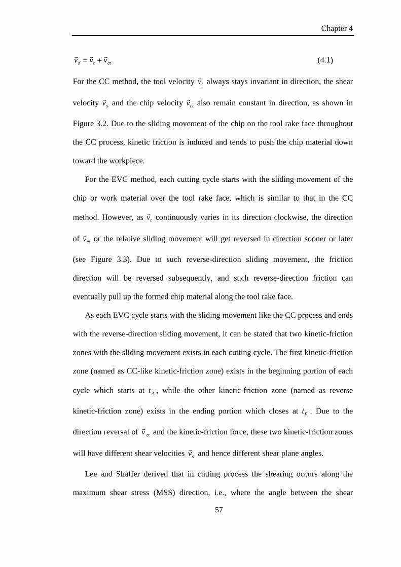
Chapter 4

57

ctts vvv += (4.1)

For the CC method, the tool velocity tv always stays invariant in direction, the shear

velocity sv and the chip velocity ctv also remain constant in direction, as shown in

Figure 3.2. Due to the sliding movement of the chip on the tool rake face throughout

the CC process, kinetic friction is induced and tends to push the chip material down

toward the workpiece.

For the EVC method, each cutting cycle starts with the sliding movement of the

chip or work material over the tool rake face, which is similar to that in the CC

method. However, as tv continuously varies in its direction clockwise, the direction

of ctv or the relative sliding movement will get reversed in direction sooner or later

(see Figure 3.3). Due to such reverse-direction sliding movement, the friction

direction will be reversed subsequently, and such reverse-direction friction can

eventually pull up the formed chip material along the tool rake face.

As each EVC cycle starts with the sliding movement like the CC process and ends

with the reverse-direction sliding movement, it can be stated that two kinetic-friction

zones with the sliding movement exists in each cutting cycle. The first kinetic-friction

zone (named as CC-like kinetic-friction zone) exists in the beginning portion of each

cycle which starts at At , while the other kinetic-friction zone (named as reverse

kinetic-friction zone) exists in the ending portion which closes at Ft . Due to the

direction reversal of ctv and the kinetic-friction force, these two kinetic-friction zones

will have different shear velocities sv and hence different shear plane angles.

Lee and Shaffer derived that in cutting process the shearing occurs along the

maximum shear stress (MSS) direction, i.e., where the angle between the shear

Chapter 4

58

velocity and the direction of resultant force is 45o ( o45=δ ) (Lee and Shaffer, 1951).

Although their model is based on an assumption of rigid-perfectly plastic work

material and neglects effects of built-up edge (BUE) and thick shear zone on the rake

face, it still gives a comprehensive physical understanding of metal cutting mechanics.

Hence, in the present study, in order to determine the shear plane angles and

boundaries of the two kinetic-friction zones, Lee and Shaffer’s slip-line solution is

extended and applied.

Based on Lee and Shaffer’s model, both the slip-line field and force relationships

for CC-like kinetic-friction zone are plotted in Figure 4.1(a). A triangular plastic

region OMN above the shear direction with the slip lines parallel or perpendicular to

OM is assumed, and the resultant force R makes 45o with the direction of the shear

force Fs. The other symbols, Fns, Fn, Fp and Ft represent the normal force

perpendicular to the shear direction, the normal force perpendicular to the rake face,

the principal force along the nominal cutting direction, and the thrust force

perpendicular to the nominal cutting direction, respectively. βk represents the kinetic-

friction angle between the tool rake face and the work material, and its value is

assumed to remain constant throughout the cutting process. According to the force

relationships in CC process (Merchant, 1945a), βk can be derived from the following

equation:

)]sincos/()sincos[(tan)/(tan 11 γγγγβ tpptnfk FFFFFF −+== −− (4.2)

Although Lee and Shaffer’s model was developed for the CC process, the same

fundamental laws of plasticity and MSS principle can also be applied to obtain the

slip-line filed for the reverse kinetic-friction zone as well. Figure 4.1(b) shows the

derived slip-line filed and the force relationships for reverse kinetic-friction zone. Due

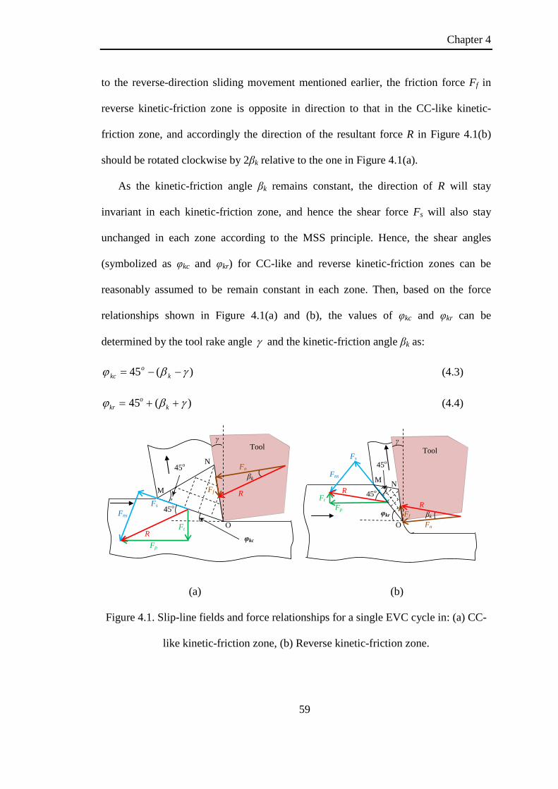
Chapter 4

59

to the reverse-direction sliding movement mentioned earlier, the friction force Ff in

reverse kinetic-friction zone is opposite in direction to that in the CC-like kinetic-

friction zone, and accordingly the direction of the resultant force R in Figure 4.1(b)

should be rotated clockwise by 2βk relative to the one in Figure 4.1(a).

As the kinetic-friction angle βk remains constant, the direction of R will stay

invariant in each kinetic-friction zone, and hence the shear force Fs will also stay

unchanged in each zone according to the MSS principle. Hence, the shear angles

(symbolized as φkc and φkr) for CC-like and reverse kinetic-friction zones can be

reasonably assumed to be remain constant in each zone. Then, based on the force

relationships shown in Figure 4.1(a) and (b), the values of φkc and φkr can be

determined by the tool rake angle γ and the kinetic-friction angle βk as:

)(45 γβϕ −−= ko

kc (4.3)

)(45 γβϕ ++= ko

kr (4.4)

45o

45o

Fs

Fns

M

O

R

Ff

βk

Tool

Fn

φkc

N

γ

Ft

Fp

R

45o

45o

R

Fs

Fns

M

N

O

Ff

Fn

βk

Tool

φkr

γ

Ft

Fp

R

(a) (b)

Figure 4.1. Slip-line fields and force relationships for a single EVC cycle in: (a) CC-

like kinetic-friction zone, (b) Reverse kinetic-friction zone.

Chapter 4

60

S

O

φkc

tv

ctv sv

Tool γ

θ

S

S′

O φs (θ)

2βk Tool

0=ctv

ts vv =

γ

(a) (b)

S′

O

θ ctv

sv φkr

Tool γ

tv

(c)

Figure 4.2. Velocity diagrams for a single EVC cycle in: (a) CC-like kinetic-friction

zone, (b) Static-friction zone, (c) Reverse kinetic-friction zone.

Given the determined shear angles, the velocity diagrams based on Equation (4.1)

for the two kinetic-friction zones can be plotted in Figure 4.2(a) and (c), where the

two dashed lines OS and OS′ represent the two constant directions of sv . In Figure

4.2(a), ctv will get close to zero when tv is approaching sv in direction. Since kinetic

friction only exists when the sliding movement occurs (i.e., ctv is not zero), in CC-

like kinetic-friction zone, the direction of tv should not rotate over OS. Otherwise, the

relative sliding movement and the chip velocity ctv may change in direction or in

Chapter 4

61

nature, and such variation could lead to the occurrence of a reverse friction direction

or another friction mode. Similar analysis can also be applied to reverse kinetic-

friction zone, where tv should not stay below OS′ in order to allow the existence of

the reverse-direction sliding movement, as shown in Figure 4.2(c). Thus, the two

shear directions OS and OS′ can be treated as the upper or lower boundaries of the

two kinetic-friction zones, respectively.

In mechanics, friction behavior can be divided into two main regimes: gross

sliding and pre-sliding, where kinetic friction and static friction dominate the process,

respectively. It is known that the kinetic friction does not immediately reverse in

direction from one gross sliding movement to the reverse-direction gross sliding

movement, and pre-sliding regime should exist as a transition zone during the reversal

process. In the EVC process, such transition zone (named as static-friction zone) acts

as an intermediate zone connecting the two kinetic-friction zones. Figure 4.2(b) shows

the velocity diagram for this transition zone, where its lower and the upper boundaries

are assumed to be determined by the obtained two shear directions in the two kinetic-

friction zones, OS and OS′. Once tv passes over OS′, the static friction will then get

converted back to kinetic friction due to the nonzero ctv and the induced gross sliding

movement. Since no gross sliding movement occurs in this pre-sliding transition

regime (i.e. 0=ctv ), according to the velocity relationship described in Equation ),

the shear velocity sv will be identical to tv in both direction and magnitude. Based on

such equivalence relation, it can be derived that the transient shear angle φs for this

transition zone is equal to the transient tool velocity angle:

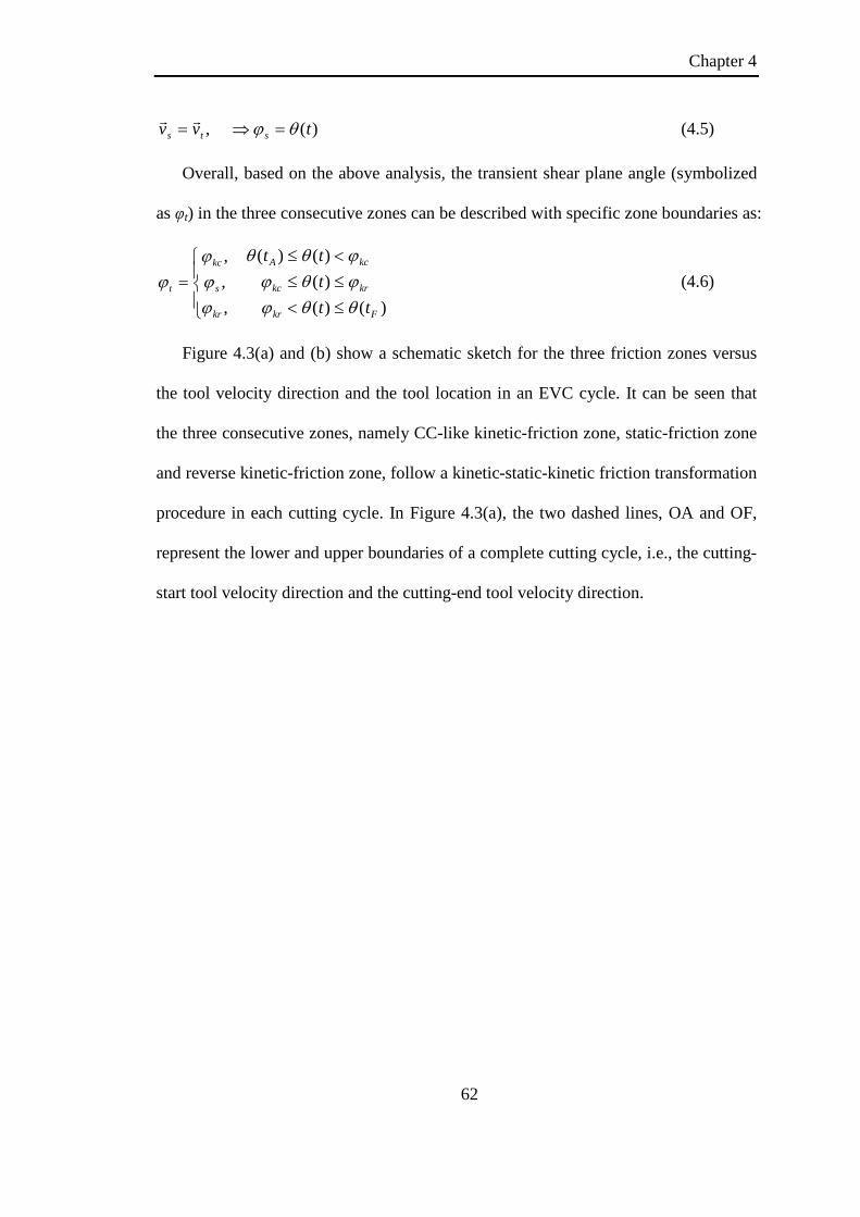
Chapter 4

62

,ts vv = )(ts θϕ =⇒ (4.5)

Overall, based on the above analysis, the transient shear plane angle (symbolized

as φt) in the three consecutive zones can be described with specific zone boundaries as:

=

,,,

kr

s

kc

t

ϕϕϕ

ϕ )()(

)()()(

Fkr

krkc

kcA

ttttt

θθϕϕθϕϕθθ

≤<≤≤<≤

(4.6)

Figure 4.3(a) and (b) show a schematic sketch for the three friction zones versus

the tool velocity direction and the tool location in an EVC cycle. It can be seen that

the three consecutive zones, namely CC-like kinetic-friction zone, static-friction zone

and reverse kinetic-friction zone, follow a kinetic-static-kinetic friction transformation

procedure in each cutting cycle. In Figure 4.3(a), the two dashed lines, OA and OF,

represent the lower and upper boundaries of a complete cutting cycle, i.e., the cutting-

start tool velocity direction and the cutting-end tool velocity direction.

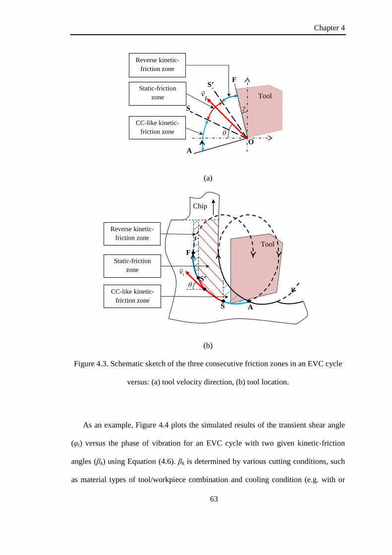
Chapter 4

63

A

tv S′

O

F

θ

S γ

Tool

CC-like kinetic-friction zone

Static-friction zone

Reverse kinetic-friction zone

(a)

A

F

tv

Tool

S′

θ

S

Chip




(b)

Figure 4.3. Schematic sketch of the three consecutive friction zones in an EVC cycle

versus: (a) tool velocity direction, (b) tool location.

As an example, Figure 4.4 plots the simulated results of the transient shear angle

(φt) versus the phase of vibration for an EVC cycle with two given kinetic-friction

angles (βk) using Equation (4.6). βk is determined by various cutting conditions, such

as material types of tool/workpiece combination and cooling condition (e.g. with or

Chapter 4

64

without coolant). The two friction angles (15o and 30o) in this figure are identified

from the friction coefficients of tungsten carbide vs tungsten carbide (0.25) and

tungsten carbide vs steel (0.6). The points A, F, S and S′ represent the cutting -start

point, the cutting-end point, and the lower and upper limits of static-friction zone,

respectively. From this figure, it can be remarked that static-friction zone plays a

significant role in the whole cutting cycle. Moreover, it can also be followed that a

smaller kinetic-friction angle can lead to comparatively i) a larger conventional shear

angle (φkc) in the CC-like kinetic-friction zone, ii) a shorter phase length in the static-

friction zone, and iii) a smaller shear angle (φkr) in the reverse kinetic-friction zone.

Such characteristic of the cutting mechanics with the EVC method looks completely

different from that with the CC method, where the latter is characterized by an

invariant shear angle through the CC process.

0

20

40

60

80

90


Tran

sien

t she

ar a

ngle

, deg


0 ... π/4 π/2

π 5π/4...2π


A S

S' F βk = 15o

βk = 30o


0 ...1/8f 1/4f 3/8f 1/2f

5/8f...1/f Time, s

3π/4

Figure 4.4. Example of transient shear angle for a cutting cycle in orthogonal EVC

process at the conditions: 0o tool rake angle, 0.094 mm/min nominal cutting speed,

vibration amplitude (a=20 µm, b=5 µm), 0.25 Hz frequency, 90o phase shift.

Chapter 4

65

4.1.3 Transient cutting force components

It is understood that the output cutting force during mechanical cutting process

highly depends on material load on the tool rake face. The higher the TOC, the higher

the material load is. Due to the variation of TOC and the variation of shear angle in

the EVC process, the cutting force gets continuously varied in each cutting cycle. In

fact, according to the illustration of TOCt in Figure 3.1, the transient force value may

start from zero at the cutting-start point A, reaches the maximum at elsewhere in the

loci and ends with zero again at the cutting-end point F. In order to derive such

transient cutting force, the famous thin shear plane model (Merchant, 1945a) is

applied and slightly modified here, and βk and τ in the EVC process are assumed to be

constant and equal to those found with the CC method.

It is known that, in the CC process, the shear force along the fixed shear plane is

calculated as:

0sintwF

cs ϕ

τ= (4.7)

where t0 is the fixed uncut chip thickness, and φc is the constant shear angle. For the

EVC process, if t0 and φc in Equation (4.7) are replaced with TOCt and φt, the

transient shear force Fs(t) can be obtained as:

tt

s TOCwtFϕ

τsin

)( = (4.8)

The value of Fs(t) can be calculated with given values of TOCt and φt, which are

determined by Equations (3.1) and (4.6), respectively.

According to Lee and Shaffer’s MSS principle (Lee and Shaffer, 1951), the angle

between the shear direction and the resultant force direction is 45o. Therefore, the

transient resultant force R(t) during cutting in each cycle can be obtained as:

Chapter 4

66

os tFtR45cos

)()( = (4.9)

Then according to the force relationships shown in Figure 4.1, the transient

principal force Fp(t) and the transient thrust force Ft(t) along the x- and y- axes, can be

derived as follows:

)45cos()()( to

p tRtF ϕ−= (4.10)

)45sin()()( to

t tRtF ϕ−= (4.11)

In order to calculate the values of these two transient cutting force components

using Equations (4.10) and (4.11), βk and τ need to be determined from the

experimental results of the orthogonal CC test. Under the CC condition, the kinetic-

friction angle, βk can be calculated from Equation (4.2) with given values of Fp and Ft,

and the shear stress τ can be derived according to the conventional thin shear plane

model (Merchant, 1945a):

)sin/())/(tancos(

0

1

c

ptc

twFFR

ϕϕ

τ−+

= , where 22pt FFR += (4.12)

where φc can be derived from the following equation (Merchant, 1945a):

γγϕ

sincostan

0

01

ttt

cc −= − (4.13)

where tc is the measured chip thickness.

With the values of βk and τ calibrated through CC tests, the transient cutting force

components for the EVC process can be subsequently calculated. Figure 4.5 shows a

flow chart of the whole calculation procedures of the transient force components

based on the proposed model.

Chapter 4

67

Give EVC conditions:cutting cond. (vc, ap, γ), and vibration cond. (a, b, f, φ)

Calculate transient thickness of cut, TOCt Calculate transient shear angle, ϕt

Calculate kinetic-friction angle, βk

Calculate shear stress, τ

Calculate transient EVC force components, R(t), Fp(t), Ft(t)

Give CC conditions and results:t0, Ft, Fp, tc, γ

Calculate constant shear angle, ϕc

Figure 4.5. Flow chart of the calculation procedures for the analytical EVC force

model.

4.2 Verification for the proposed model

In this section, the proposed analytical force model for the orthogonal EVC

process is experimentally validated. Using the calibrated parameters, the proposed

force model is employed to predict values of the transient cutting force components,

and these values are compared with the experimental force values obtained from the

EVC test.

4.2.1 Calibration for the parameters

An orthogonal CC test (i.e., without the tool vibration) is conducted to calibrate

the two important parameters (τ and βk). Table 4.1 shows detailed conditions for the

orthogonal CC test, and the experimental set-up can be seen in Figure 3.8.

Chapter 4

68

Table 4.1. Cutting and vibration conditions for the orthogonal CC test.

Uncut chip thickness, t0 [µm] 15 Width of cut, w [µm] 400 Cutting speed, [mm/min] 0.188 Lubrication condition Dry cutting

For the orthogonal CC test, Figure 4.6(a) shows the recorded values of the cutting

force components, and Figure 4.6(b) shows the microscope photograph of the formed

chip in the CC process. Based on the experimental results, the average thrust force Ft

and the average principal force Fp were calculated to be 0.4 N and 6.6 N, respectively.

The average thickness of the generated chip, tc is measured to be about 41 µm.

Therefore, by substituting the values of Ft, Fp, tc, w and t0 into Equations (4.2), (4.12)

and (4.13), the constant shear angle φc is calculated to be 20o, and the values of βk and

τ for the CC condition are found to be 3.46o and 347 MPa, respectively.

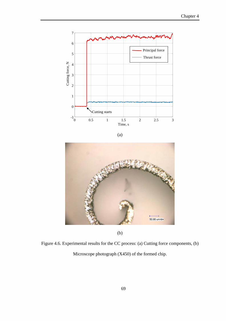
Chapter 4

69

0 0.5 1 1.5 2 2.5 3

-1

0

1

2

3

4

5

6

7

Time, s

Cut

ting

forc

e, N

Principal force

Thrust force

Cutting starts

(a)

(b)

Figure 4.6. Experimental results for the CC process: (a) Cutting force components, (b)

Microscope photograph (X450) of the formed chip.

Chapter 4

70

4.2.2 Validation for the developed model

By following the calculation method shown in Figure 4.5, the transient cutting

forces are calculated given the cutting and vibration conditions listed in Table 4.1 and

the calibrated two parameters βk and τ. As stated in Chapter 3, according to the

existing studies (Nath et al., 2011; Shamoto et al., 2008), speed ratio is considered as

one of the most essential parameters in the EVC method (Nath et al., 2011; Shamoto

et al., 2008). Therefore, in the orthogonal EVC tests, different speed ratios are

employed to study the applicability of the proposed model. The experimental transient

cutting force values can be obtained from Chapter 3.

Figure 4.7 shows the comparison between the predicted and experimental

maximum transient resultant forces, Rmax, at the four different speed ratios. It can be

seen that both the predicted and experimental values of Rmax increase with the

increment of speed ratio. The comparison results in Figure 4.7 shows that the

predicted values of Rmax correspond well with the experimental values, indicating that

the effect of different speed ratios on transient cutting force can be effectively

predicted by the proposed force model.

Chapter 4

71

0

1

2

3

4

5

6

0.025 0.05 0.75 0.1Speed ratio, R s

Max

imum

resu

ltant

forc

e, R

max

, N

Expe. ValuePred. value

Figure 4.7. Experimental and predicted maximum transient resultant cutting force

with different speed ratios.

As an example, Figure 4.8 shows the predicted transient principal and thrust force

(i.e. Fp(t) and Ft(t)) with the four speed ratios (0.025, 0.05, 0.075 and 0.1), and the

retrieved experimental force values are superimposed in the same figure for

comparison. It can be seen from Figure 4.8 that the transient principle force first

increases due to the increasing TOCt (see Figure 3.1), then decreases slightly due to

both the increasing φt (see Figure 4.4) and the decreasing TOCt, and finally drops to

zero after the disengagement of tool and chip. For the predicted principal force, it can

be noticed that its variation trend and zero-to-peak value correspond well with those

of the experimental one.

It can also be noticed from Figure 4.8 that the transient thrust force first starts

increasing from zero to a maximum positive value, but then gradually decreases to

negative values, indicating that the tool is pulling the chip or work material upward

Chapter 4

72

from the workpiece. Such unique phenomenon which is completely different from the

CC process is caused by the friction reversal in each cutting cycle of the EVC process.

From Figure 4.8, it can also be observed that the predicted cutting-end point (the

point where the principal or the thrust force becomes zero) does not agree with the

experimental one, indicating that the tool still stays engaged with the work or chip

material after passing over the theoretical cutting-end point. This kind of disaccord is

considered to be caused by elastic recovery of either the work or the chip material at

this stage. That means when the tool edge passes the theoretical cutting-end, the work

or chip material will gradually rebound elastically with the receding movement of the

tool, until its elastic energy is completely released and it is truly disengaged from the

tool rake face.

Chapter 4

73


0

1

2

3

4

5

-1

Forc

e, N

Pred. force

Expt. force

0 π/2 π 3π/2 2π

Principal force

Thrust force

0 -1

0

1

2

3

4

5


Forc

e, N

Thrust force

Principal force

π/2 π 3π/2 2π

Pred. force

Expt. force

(a) Rs= 0.025 (b) Rs= 0.05

Phase of vibration, rad 0 π/2

π

3π/2

2π

Forc

e, N

0

1

2

3

4

5

-1

Pred. force

Expt. force

Principal force

Thrust force

0 π/2 π 3π/2 2π


Forc

e, N

0

1

2

3

4

5

-1

Pred. force

Expt. force

Principal force

Thrust force

(c) Rs= 0.075 (d) Rs= 0.1

Figure 4.8. Experimental and predicted transient cutting force components for an

EVC cycle.

4.3 Concluding Remarks

In this chapter, an analytical force model for orthogonal EVC process has been

developed for in-depth understanding of the transient cutting mechanics and for

accurate prediction of the transient cutting force components. Based on this study, the

following conclusions can be drawn:

Chapter 4

74

• By analyzing transition characteristic of friction reversal in the EVC process,

static friction is considered to exist in the transition zone between the two kinetic-

friction zones. Based on variation of the friction modes, each cutting cycle is

divided into three consecutive zones: CC-like kinetic-friction zone, static-friction

zone and reverse kinetic-friction zone.

• Transient shear angles for the three friction zones are derived by investigating

the velocity relationship and employing the Lee and Shaffer’s slip-line solution in

the EVC process. Mathematical simulation shows that the static-friction zone

plays an important role in the transient shear angle and the cutting force values in

each cutting cycle.

• The predicted transient cutting force values are found to be in good agreement

with the recorded experimental data in the orthogonal EVC tests conducted on

6061 aluminum alloy at four different speed ratios.

• The proposed analytical force model can express the EVC mechanism more

finely, and assist to predict more accurate cutting force values, and is supposed to

be helpful for researchers to proceed with further study on the EVC technique.

Chapter 5

75

Chapter 5: Experimental and analytical

studies of surface generation in EVC

As discussed in Chapter 2, it is already known that some of the characteristics of

the EVC method are fundamentally different from the CC and CVC methods, which

are considered to be main reasons for the superior performance of the EVC method.

However, during the EVC process, vibration marks or cusps are formed on the

machined surface profile along the nominal cutting direction. Such cusps, which are

generated by the elliptical vibration trajectory and will increase the overall roughness

of machined surface, are considered to be detrimental for achieving high-quality

surface and a major disadvantage for EVC. In order to suppress the vibration marks

and decrease the surface roughness, a very low nominal cutting speed needs to be

employed to enhance the overlapping of the elliptical vibration locus, which can result

in longer machining time and lower production efficiency.

Regarding the surface generation in the EVC process, Shamoto et al. proposed a

method to predict the height of the vibration marks assuming a perfectly sharp tool

edge, as described in Chapter 2. However, until now, very little research has been

conducted to study the effects of machining and vibration parameters on surface

generation. Furthermore, it is well known that the tool edge can never be perfectly

sharp, and the tool edge radius usually ranges from tens of nanometers (e.g. SCD tool)

to several microns (e.g. PCD tool, high-speed steel tool). As the vibration amplitudes

of the EVC method are usually at micron-level, the effect of tool edge radius is

Chapter 5

76

probably significant, especially for those non-SCD tools of which the edge radius is

comparable to the vibration amplitudes.

Hence, in this chapter, in order to understand the surface generation process along

nominal cutting direction, an experimental study comprising a series of grooving tests

using a SCD tool with the EVC method is carried out firstly. The effects of nominal

cutting speed on the surface generation at two different thrust-directional vibration

amplitudes are investigated. Secondly, an analytical model for the surface generation

along the nominal cutting direction is developed. Considering the geometrical

relationship, the effect of tool edge radius on the surface generation is mathematically

investigated. Finally, the proposed surface generation model is experimentally

verified by conducting a series of grooving tests on soft and hard work materials using

a PCD tool with the EVC method.

5.1 Experimental study using the SCD tool

5.1.1 Experimental setup

According to the theoretical analysis in Section 2.1.2, it can be noted that the

theoretical roughness Rth is determined by the vibration parameters (a, b, ω and φ )

and the nominal cutting speed (vc). However, during a practical cutting test, the

vibration parameters are preset before machining starts, and all these vibration

parameters are usually kept constant during an individual machining test. Thus, in this

study, the surface generation at different nominal cutting speeds is studied.

Furthermore, as the thrust-directional amplitude b is directly proportional to Rth and

plays an important factor (see Equation (2.17)), two different values of b are applied

in the tests.

Chapter 5

77

A series of grooving tests were conducted using an elliptical vibration device,

which is attached to the tool-post of the 4-axis CNC ultraprecision machine. The

vibrator vibrates at a frequency f of 38.87 kHz, with a phase difference ϕ of 90o. All

the grooving test conditions under the EVC method are shown in Table 5.1. Six

nominal cutting speeds ranging from 1 m/min to 6 m/min are applied, with the

corresponding speed ratio ranging from 0.03 to 0.24. The workpiece is made of 6061

aluminum alloy, and a fresh SCD tool is set at the specific tool position of the vibrator

with the nose radius of 0.6 mm and the rake, flank and approach angles of 0o, 7o and

30o.

Table 5.1. Conditions of the grooving test

Vibration amplitude, [µm] a 2

b 2 1

Depth of cut, [µm] 5 Nominal cutting speed, vc, [m/min] 1 2 3 4 5 6 Speed ratio, Rs 0.03 0.07 0.10 0.13 0.17 0.24

5.1.2 Results and analysis

Figure 5.1 shows microscope photographs of the machined grooves at the six

different nominal cutting speeds. It can be observed that, when the nominal cutting

speed is less than or equal to 2 m/min, the vibration marks are insignificant and

difficult to notice, and they become more and more obvious with the increase in the

nominal cutting speed. The reason for such phenomenon lies in that the height of

vibration marks gets increased with the increase in vc, according to Equations (2.15)

and (2.17).

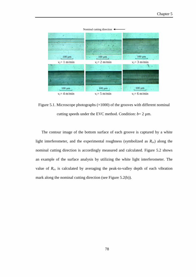
Chapter 5

78

100 µm 100 µm 100 µm

vc= 1 m/min vc= 2 m/min vc= 3 m/min

100 µm 100 µm 100 µm

vc= 4 m/min vc= 5 m/min vc= 6 m/min


Figure 5.1. Microscope photographs (×1000) of the grooves with different nominal

cutting speeds under the EVC method. Condition: b= 2 µm.

The contour image of the bottom surface of each groove is captured by a white

light interferometer, and the experimental roughness (symbolized as Rex) along the

nominal cutting direction is accordingly measured and calculated. Figure 5.2 shows

an example of the surface analysis by utilizing the white light interferometer. The

value of Rex is calculated by averaging the peak-to-valley depth of each vibration

mark along the nominal cutting direction (see Figure 5.2(b)).

Chapter 5

79

(a) (b) Figure 5.2. Example of surface analysis by a white light interferometer. (a) Contour

image of the groove bottom, (b) Surface profile along the nominal cutting direction.

Conditions: vc= 6 m/min, b= 2 µm.

With the known vibration and machining parameters (a, b, ω, φ , and vc), the

theoretical roughness value at the six different nominal cutting speeds can be

calculated based on Equations (2.15) and (2.17). Figure 5.3 shows the comparison

results between Rex and Rth at the two different thrust-directional amplitudes. It should

be noted that the vertical scale of Figure 5.3(a) is two times that of Figure 5.3(b), due

to the proportional relationship between b and Rth (see Equation (2.17)). From Figure

5.3(a), it can be seen that Rex starts to be detectable and becomes a significant value,

as vc is set larger than 2 m/min at 2 µm thrust-directional amplitude. In Figure 5.3(b),

a similar critical vc is found to be 3 m/min at 1 µm thrust-directional amplitude. As vc

is smaller than or equal to 2 m/min or 3 m/min, the value of Rex is quite small,

typically less than 10 nm. The reason for such phenomenon may lie in the non-zero

edge radius of the SCD tool, which has not been considered in the roughness model

stated earlier. Although an SCD tool usually has an edge radius of submicron level

(ranging from tens to hundreds of nanometers), it is still relatively large when

considering the feature generation of submicron or even nanometer level. Due to the

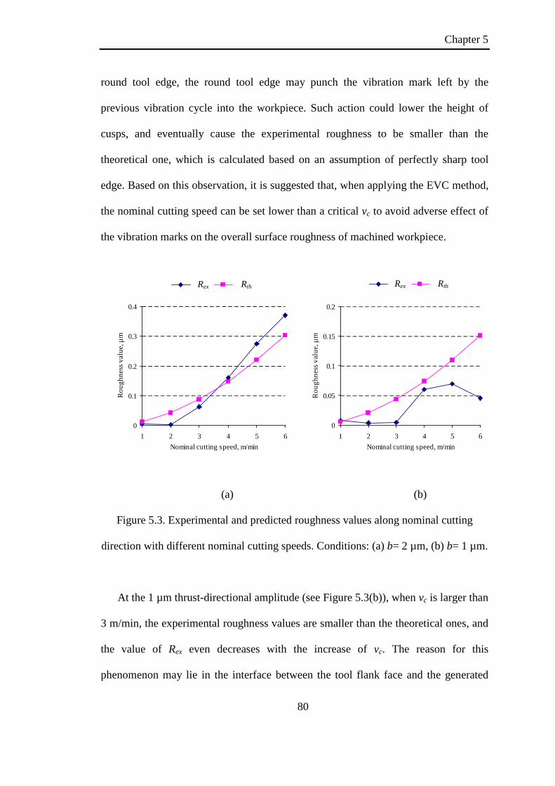
Chapter 5

80

round tool edge, the round tool edge may punch the vibration mark left by the

previous vibration cycle into the workpiece. Such action could lower the height of

cusps, and eventually cause the experimental roughness to be smaller than the

theoretical one, which is calculated based on an assumption of perfectly sharp tool

edge. Based on this observation, it is suggested that, when applying the EVC method,

the nominal cutting speed can be set lower than a critical vc to avoid adverse effect of

the vibration marks on the overall surface roughness of machined workpiece.

(a) (b)

Figure 5.3. Experimental and predicted roughness values along nominal cutting

direction with different nominal cutting speeds. Conditions: (a) b= 2 µm, (b) b= 1 µm.

At the 1 µm thrust-directional amplitude (see Figure 5.3(b)), when vc is larger than

3 m/min, the experimental roughness values are smaller than the theoretical ones, and

the value of Rex even decreases with the increase of vc. The reason for this

phenomenon may lie in the interface between the tool flank face and the generated

0

0.05

0.1

0.15

0.2

1 2 3 4 5 6Nominal cutting speed, m/min

Rou

ghne

ss v

alue

, µm

Expt. Pred.

0

0.1

0.2

0.3

0.4

1 2 3 4 5 6Nominal cutting speed, m/min

Rou

ghne

ss v

alue

, µm

Expe. Pred. Rth Rex Rth Rex

Chapter 5

81

vibration marks, which has not been considered in the roughness model as stated in

Section 2.1.2.

5.2 Development of the surface generation model considering tool edge

radius

It is well known that, during precision or micro machining process, the surface

generation mechanism is considered to be significantly affected by the tool

microgeometry parameters (Liu et al., 2007) (e.g. the tool edge radius). During the

EVC process, since the vibration amplitudes of the EVC method are usually at

micron-level (Brehl and Dow, 2008), the tool edge dimension of most kinds of tools

(except the SCD tool) is usually comparable to the vibration amplitudes and hence has

significant effect on the surface generation mechanism. Therefore, the tool edge

dimension must be considered while predicting the surface roughness for the EVC

process.

The geometry of a cutting tool is defined by several tool parameters, such as nose

radius, rake angle, clearance angle λ and edge radius re. In this study, the tool edge is

assumed to be round, and the cross-section of the cutting tool can be schematically

illustrated with a basic geometry as shown in Figure 5.4. The points To and Tb

represent the center of the tool edge circle and the bottom point of tool edge,

respectively.

Chapter 5

82


Rake face

re

λ

Flank face

Tb

To

Figure 5.4. Schematic cross-section view of tool geometry.

For a tool with a round tool edge, the surface generation point T (i.e. the point

where the tool edge contacts the finished surface profile) continuously varies along

the round tool edge during each EVC cycle. Figure 5.5 shows the surface generation

process using the round edge tool applying the EVC method. The dash line curve A-

B-C in Figure 5.5 represents the vibration trajectory of the bottom point Tb of the

round tool edge (see Figure 5.4). According to the nature of surface generation

mechanism, it can be found that at any location where the machined surface is

generated, the tool edge circle will be always tangent to the generated surface profile.

It means that the finished surface profile is actually generated by an envelope line of

the round tool edge, which eventually results in a solid curve Ae-Be-Ce, as shown in

Figure 5.5. The points Ae and Ce represent cross-over points for the two consecutive

envelope lines of the round tool edge. The point Be represents the bottom point of the

theoretically machined surface considering the round tool edge and has the same

coordinate value with the bottom point B of the elliptical vibration trajectory (see

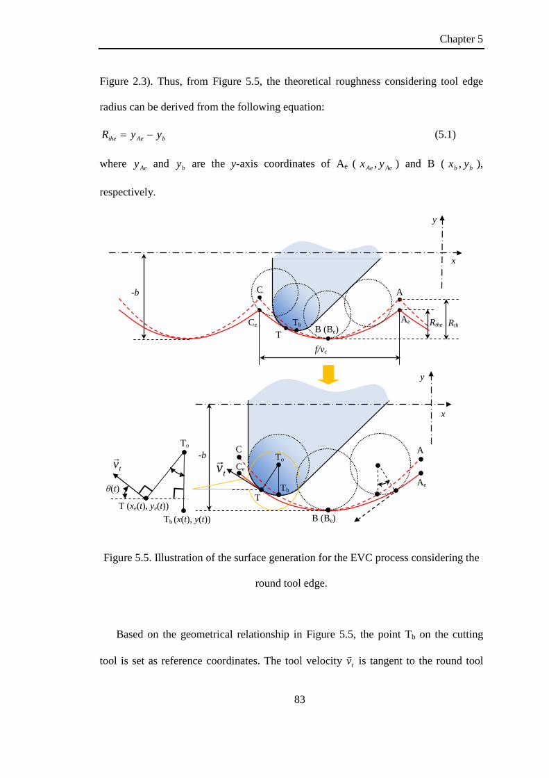
Chapter 5

83

Figure 2.3). Thus, from Figure 5.5, the theoretical roughness considering tool edge

radius can be derived from the following equation:

bAethe yyR −= (5.1)

where Aey and by are the y-axis coordinates of Ae ( AeAe yx , ) and B ( bb yx , ),

respectively.

-b C

x

y

B (Be)

A

Rth Rthe Ce Ae T

Tb

f/vc

C

B (Be)

A

Ce

Ae T

Tb

To

tv

x

y

-b

To

Tb (x(t), y(t)) T (xe(t), ye(t))

tv

θ(t)

Figure 5.5. Illustration of the surface generation for the EVC process considering the

round tool edge.

Based on the geometrical relationship in Figure 5.5, the point Tb on the cutting

tool is set as reference coordinates. The tool velocity tv is tangent to the round tool

Chapter 5

84

edge, which is perpendicular to the radial line ToT of the edge circle, as shown in

Figure 5.5. Then, it can be derived that the angle boTTT∠ is equal to the transient tool

velocity angle )(tθ . Hence, the coordinates of the transient surface generation point T

( )(),( tytx ee ) on the curve Ae-Be-Ce can be calculated based on the relative position

between T and Tb:

−+=−=

))(cos1()()()(sin)()(

trtytytrtxtx

ee

ee

θθ

−++=−−=

⇒))(cos1()cos()(

)(sin)cos()(trtbty

trtvtatx

ee

ece

θφωθω

(5.2)

If Aet and Cet are used to represent the time instants when the surface generation

point T passes the cross-over points Ae ( )(),( AeeAee tytx ) and Ce ( )(),( CeeCee tytx ), by

substituting Equation (5.2) into Equation (5.1), the following equation can be derived:

)()( btyR Aeethe −−=

btrtbR AeeAethe +−++=⇒ ))(cos1()cos( θφω (5.3)

It can be noticed from the Equation (5.3) that the theoretical roughness value can

be determined, if the value of Aet is obtained. As the pitch of the regular wave is

equal to the distance which is given by the total relative movement of the tool and the

workpiece in the cutting direction from Aet to Cet , the following equation can be

derived:

ωπ cCeeAee vtxtx 2)()( =− (5.4)

In addition, it is also understood that the vertical positions of the crossover points

Ae and Ce are equal. Hence,

Chapter 5

85

0)()( =− CeeAee tyty (5.5)

By substituting Equation (5.2) into Equations (5.4) and (5.5), the following

equation set can be derived:

=−++−−++=−−−−−

0))(cos1()cos())(cos1()cos(2)(sin)cos()(sin)cos(

CeeCeAeeAe

cCeeCecCeAeeAecAe

trtbtrtbvtrtvtatrtvta

θφωθφωωπθωθω

(5.6)

In order to solve the above equation set, Equation (5.6) needs to be refined into an

equation set with two variables Aet and Cet . According to Equations (2.10) and (2.11),

)(sin tθ and )(cos tθ can be derived from the following equations:

+

−=

+

′=

22

22

)(')('

)(')(cos

)(')('

)()(sin

tytxtxt

tytxtyt

θ

θ

+++

+=

+++

+−=

⇒

22

22

))sin(())sin((

)sin()(cos

))sin(())sin((

)sin()(sin

φωωωω

ωωθ

φωωωω

φωωθ

tbvta

vtat

tbvtatbt

c

c

c

(5.7)

Finally, by substituting Equation (5.7) into Equation (5.6), a nonlinear equation

set can be derived as follows:

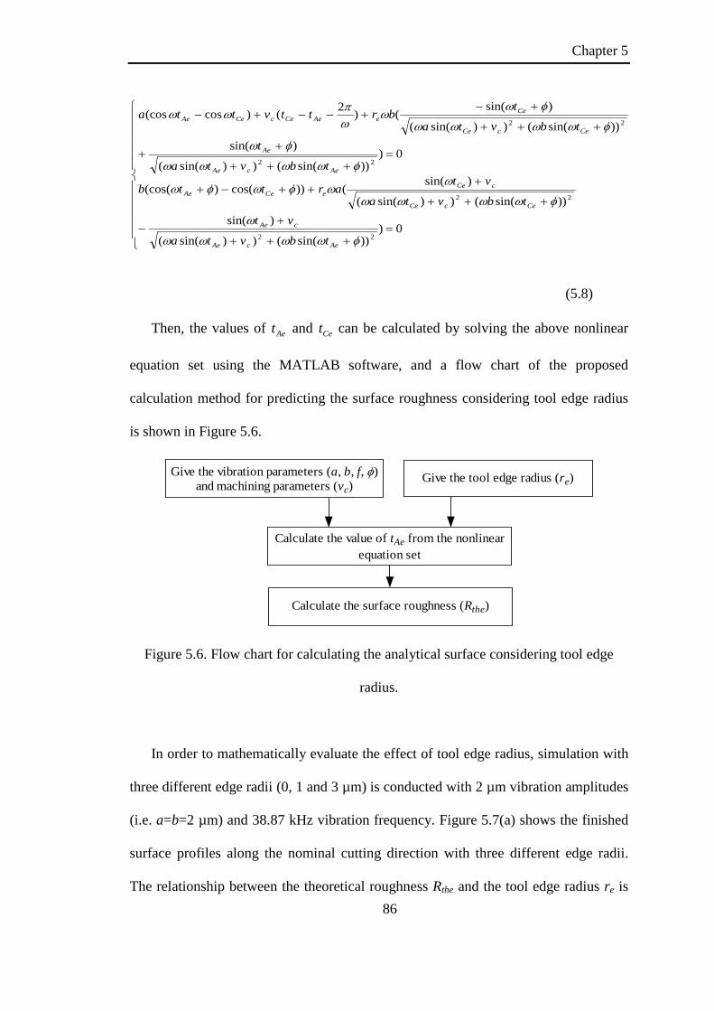
Chapter 5

86

=+++

+−

+++

+++−+

=+++

++

+++

+−+−−+−

0)))sin(())sin((

)sin())sin(())sin((

)sin(())cos()(cos(

0)))sin(())sin((

)sin())sin(())sin((

)sin(()2()cos(cos

22

22

22

22

φωωωω

ωφωωωω

ωωφωφω

φωωωω

φωφωωωω

φωω

ωπωω

AecAe

cAe

CecCe

cCeeCeAe

AecAe

Ae

CecCe

CeeAeCecCeAe

tbvta

vttbvta

vtarttb

tbvta

ttbvta

tbrttvtta

(5.8)

Then, the values of Aet and Cet can be calculated by solving the above nonlinear

equation set using the MATLAB software, and a flow chart of the proposed

calculation method for predicting the surface roughness considering tool edge radius

is shown in Figure 5.6.

Give the vibration parameters (a, b, f, φ)and machining parameters (vc)

Calculate the value of tAe from the nonlinearequation set

Give the tool edge radius (re)

Calculate the surface roughness (Rthe)

Figure 5.6. Flow chart for calculating the analytical surface considering tool edge

radius.

In order to mathematically evaluate the effect of tool edge radius, simulation with

three different edge radii (0, 1 and 3 µm) is conducted with 2 µm vibration amplitudes

(i.e. a=b=2 µm) and 38.87 kHz vibration frequency. Figure 5.7(a) shows the finished

surface profiles along the nominal cutting direction with three different edge radii.

The relationship between the theoretical roughness Rthe and the tool edge radius re is

Chapter 5

87

shown in Figure 5.7(b). It can be observed that Rthe decreases gradually with the

increase of re. The theoretically rough finished surface profile is generated by the

perfectly-sharp tool. It can also be foreseen that, without considering the effect of

elastic recovery and material side flow, if the tool edge radius becomes infinitely large,

the theoretical roughness Rthe will approach to be zero.

-3.5 -3 -2.5 -2 -1.5 -1 -0.5 0 0.5

-2.1

-2

-1.9

-1.8

-1.7

-1.6

x, µm

y, µ

m

re = 0 µm re = 1 µm re = 3 µm

(a)

0 1 2 3 4 5 6 7 8 9 10

0

0.02

0.04

0.06

0.08

0.1

Tool edge radius re, µm

Theo

retic

al ro

ughn

ess R

the,

µm

(b)

Figure 5.7. (a) Simulated surface profiles along the nominal cutting direction

considering tool edge radius for the EVC process, (b) Theoretical roughness versus

tool edge radius. Conditions: 3 m/min nominal cutting speed; circular vibration with 2

µm amplitude; 38.87 kHz vibration frequency.

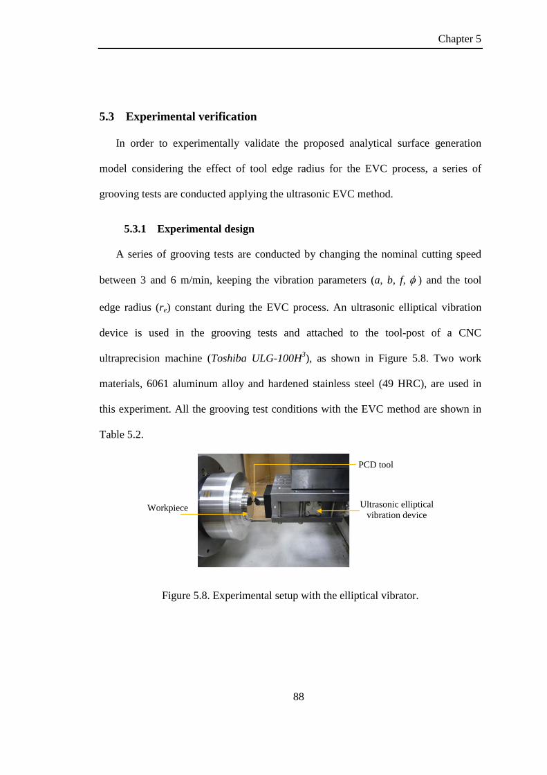
Chapter 5

88

5.3 Experimental verification

In order to experimentally validate the proposed analytical surface generation

model considering the effect of tool edge radius for the EVC process, a series of

grooving tests are conducted applying the ultrasonic EVC method.

5.3.1 Experimental design

A series of grooving tests are conducted by changing the nominal cutting speed

between 3 and 6 m/min, keeping the vibration parameters (a, b, f, φ ) and the tool

edge radius (re) constant during the EVC process. An ultrasonic elliptical vibration

device is used in the grooving tests and attached to the tool-post of a CNC

ultraprecision machine (Toshiba ULG-100H3), as shown in Figure 5.8. Two work

materials, 6061 aluminum alloy and hardened stainless steel (49 HRC), are used in

this experiment. All the grooving test conditions with the EVC method are shown in

Table 5.2.

Workpiece Ultrasonic elliptical vibration device

PCD tool

Figure 5.8. Experimental setup with the elliptical vibrator.

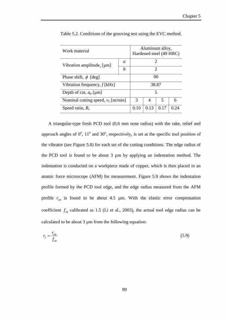
Chapter 5

89

Table 5.2. Conditions of the grooving test using the EVC method.

Work material Aluminum alloy, Hardened steel (49 HRC)

Vibration amplitude, [µm] a 2

b 2

Phase shift, φ [deg] 90

Vibration frequency, f [kHz] 38.87

Depth of cut, ap [µm] 5

Nominal cutting speed, vc [m/min] 3 4 5 6

Speed ratio, Rs 0.10 0.13 0.17 0.24

A triangular-type fresh PCD tool (0.6 mm nose radius) with the rake, relief and

approach angles of 0o, 11o and 30o, respectively, is set at the specific tool position of

the vibrator (see Figure 5.8) for each set of the cutting conditions. The edge radius of

the PCD tool is found to be about 3 µm by applying an indentation method. The

indentation is conducted on a workpiece made of copper, which is then placed in an

atomic force microscope (AFM) for measurement. Figure 5.9 shows the indentation

profile formed by the PCD tool edge, and the edge radius measured from the AFM

profile emr is found to be about 4.5 µm. With the elastic error compensation

coefficient sbf calibrated as 1.5 (Li et al., 2003), the actual tool edge radius can be

calculated to be about 3 µm from the following equation:

sb

eme f

rr = (5.9)

Chapter 5

90

0 3164 [nm] 0

158

[nm]

Figure 5.9. AFM analysis of the PCD tool edge indentation.

5.3.2 Experimental results

Figure 5.10(a) and (b) show the microscope photographs of the machined grooves

at 6 m/min nominal cutting speed on the workpieces made of aluminum alloy and

hardened steel.

100 µm 100 µm


(a) (b)

Figure 5.10. Microscope photographs (×1000) of the machined grooves under the

EVC method on the workpieces made of: (a) Aluminum alloy, (b) Hardened steel.

The experimental roughness Rex under the test conditions is measured using a

white light interferometer, and the value is calculated by averaging the peak-to-valley

depth of each vibration mark along the nominal cutting direction. Figure 5.11 shows

Chapter 5

91

the surface roughness measurement of the aluminum alloy groove using the white

light interferometer at 6 m/min nominal cutting speed.



x, µm

y,µm

36 38 40 42

-0.8

-0.7

-0.6

-0.5

-0.4

-0.3

Figure 5.11. Surface roughness measurement using the white light interferometer.

Condition: 6 m/min nominal cutting speed.

Given the vibration and machining parameters (a, b, f, φ and vc), the theoretical

roughness considering the edge radius can be calculated using Equations (5.3) and

(5.8). Figure 5.12 shows a comparison between the predicted roughness along the

nominal cutting direction and the experimentally measured roughness (Rex) on the

aluminum alloy and hardened steel workpieces. As shown in Figure 5.12, both the

predicted and experimental roughness increases gradually with the increment of

nominal cutting speed. It is because that, with the increase of cutting speed, the

elliptical vibration locus becomes less overlapping along the nominal cutting direction,

and the height of vibration marks will increase.

Chapter 5

92

It can be seen from Figure 5.12 that Rthe considering the edge radius (re=3 µm)

corresponds well with the experimentally measured roughness Rex, which

demonstrates that the proposed surface generation model performs well in predicting

the roughness along the nominal cutting direction in the EVC process. Meanwhile, it

can also be seen that the predicted roughness Rth without considering the edge radius

(re=0 µm) is significantly larger than Rex of both materials at all the nominal cutting

speeds. Such discrepancy is caused by the overlook of the round tool edge, which can

lower the height of the vibration marks compared to a perfectly-sharp cutting tool.

0

0.1

0.2

0.3

0.4

3 4 5 6Nominal cutting speed, m/min

Rou

ghne

ss v

alue

, µm

Rth

Re

Expe. (Fe)

Expe. (Al)

Rth (re= 0 µm)

Rthe (re= 3 µm)

Rex (re≈ 3 µm, Hardened steel) Rex (re≈ 3 µm, Aluminum alloy)

Figure 5.12. Experimental and predicted roughness along nominal cutting direction

with different nominal cutting speeds.

It is known that, in conventional micromachining, minimum uncut chip thickness

is important when predicting the surface roughness due to the size effect (Liu et al.,

2007). However, in elliptical-vibration-assisted micromachining, periodic motion of

the tool exists along the thrust direction in each EVC cycle (see Figure 2.2). Such

unique movement will help the uncut material to realize plastic deformation and assist

the chip to flow away from the workpiece surface. This fact will mitigate the effect of

Chapter 5

93

minimum chip thickness and make it insignificant and negligible in the EVC process.

Therefore, the pure geometrical model can evaluate the surface roughness well, even

without considering the minimum chip thickness.


An experimental study comprising a series of grooving tests using an SCD tool is

carried out to deeply understand the surface generation process along nominal cutting

direction under the EVC method, and a comprehensive surface generation model for

the EVC method has been developed for in-depth understanding of the effect of tool

edge radius on predicting the surface roughness along nominal cutting direction. The

following conclusions can be drawn based on this study:

• There exists a critical nominal cutting speed for different thrust amplitudes,

below which the experimental roughness is quite small and the vibration marks

are almost undetectable.

• Mathematical evaluation reveals that the tool edge radius should not be

overlooked for more accurate roughness prediction along the nominal cutting

direction. The simulation results show that the theoretical roughness decreases

with the increase of the tool edge radius. It is because that the height of the

vibration marks generated by a tool with a larger edge radius is smaller than that

generated by a tool with a smaller edge radius.

• The predicted roughness along the nominal cutting direction based on the

proposed model is found to be in significantly better agreement with the

measured experimental roughness of both materials than the predicted values

without considering tool edge radius.

Chapter 6

94

Chapter 6: Ultrasonic EVC of hardened

stainless steel using PCD tools

Hardened steel has been widely used in die and mold parts for producing mainly

plastic lenses. Hence, direct machining of the hardened steel, which is cost-effective,

to obtain high-quality surface is always a concern of industries. Instead of grinding

and polishing, direct ultraprecision machining of this material would save

considerable machining time and cost. However, steel becomes more brittle and less

ductile after it is hardened, making the workpiece difficult to cut using the CC method.

It is known that SCD tools have been widely used to cut non-ferrous materials to

achieve high-quality mirror surface in ultraprecision engineering due to their high

hardness, long tool life and low thermal conductivity. However, directly machining of

steel using the CC method is impossible, due to the excessive tool wear caused by the

strong chemical affinity between carbon and iron atoms.

As described in Chapter 2, Moriwaki et al. have justified the feasibility of

achieving optical quality mirror surface by applying the CVC method using SCD

tools (Moriwaki and Shamoto, 1991). EVC has been proved to be a promising method

in terms of almost all cutting performances compared to the CC and CVC methods in

cutting and grooving of hardened steel. Shamoto et al. have used SCD tools to

machine hardened steel by applying the EVC method, and found extremely smaller

cutting force and much longer tool life compared to the CC and CVC methods. As an

inexpensive artificial diamond tool compared to SCD, PCD has been proved as a

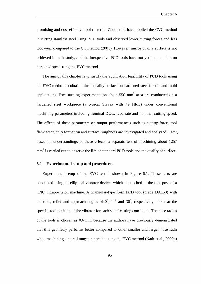
Chapter 6

95

promising and cost-effective tool material. Zhou et al. have applied the CVC method

in cutting stainless steel using PCD tools and observed lower cutting forces and less

tool wear compared to the CC method (2003). However, mirror quality surface is not

achieved in their study, and the inexpensive PCD tools have not yet been applied on

hardened steel using the EVC method.

The aim of this chapter is to justify the application feasibility of PCD tools using

the EVC method to obtain mirror quality surface on hardened steel for die and mold

applications. Face turning experiments on about 550 mm2 area are conducted on a

hardened steel workpiece (a typical Stavax with 49 HRC) under conventional

machining parameters including nominal DOC, feed rate and nominal cutting speed.

The effects of these parameters on output performances such as cutting force, tool

flank wear, chip formation and surface roughness are investigated and analyzed. Later,

based on understandings of these effects, a separate test of machining about 1257

mm2 is carried out to observe the life of standard PCD tools and the quality of surface.

6.1 Experimental setup and procedures

Experimental setup of the EVC test is shown in Figure 6.1. These tests are

conducted using an elliptical vibrator device, which is attached to the tool-post of a

CNC ultraprecision machine. A triangular-type fresh PCD tool (grade DA150) with

the rake, relief and approach angles of 0o, 11o and 30o, respectively, is set at the

specific tool position of the vibrator for each set of cutting conditions. The nose radius

of the tools is chosen as 0.6 mm because the authors have previously demonstrated

that this geometry performs better compared to other smaller and larger nose radii

while machining sintered tungsten carbide using the EVC method (Nath et al., 2009b).

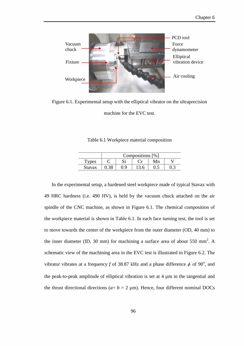
Chapter 6

96

Vacuum chuck Fixture

Workpiece

PCD tool Force dynamometer Elliptical vibration device

Air cooling

Figure 6.1. Experimental setup with the elliptical vibrator on the ultraprecision

machine for the EVC test.

Table 6.1 Workpiece material composition

Compositions [%] Types C Si Cr Mn V Stavax 0.38 0.9 13.6 0.5 0.3

In the experimental setup, a hardened steel workpiece made of typical Stavax with

49 HRC hardness (i.e. 490 HV), is held by the vacuum chuck attached on the air

spindle of the CNC machine, as shown in Figure 6.1. The chemical composition of

the workpiece material is shown in Table 6.1. In each face turning test, the tool is set

to move towards the center of the workpiece from the outer diameter (OD, 40 mm) to

the inner diameter (ID, 30 mm) for machining a surface area of about 550 mm2. A

schematic view of the machining area in the EVC test is illustrated in Figure 6.2. The

vibrator vibrates at a frequency f of 38.87 kHz and a phase difference φ of 90o, and

the peak-to-peak amplitude of elliptical vibration is set at 4 µm in the tangential and

the thrust directional directions (a= b = 2 µm). Hence, four different nominal DOCs

Chapter 6

97

of 2, 4, 6 and 10 µm are chosen. During the face turning, the nominal cutting speed

decreases while the tool moves towards the centre due to the traverse feed:

vc=2πrnr/60 (6.1)

where nr is the spindle rotational speed, r is the radial distance from the workpiece

center. Earlier, Nath et al. have theoretically and experimentally demonstrated that a

significantly reduced value of the maximum thickness of cut could be achieved when

the speed ratio is set lower than the critical speed ratio of 0.12837 (Nath et al., 2011).

Hence three different speed ratios, where two values are smaller and larger than

0.12837 and the other value is approximately equal to 0.12837, are chosen by varying

the spindle speed. Then at a fixed nominal DOC and a fixed spindle speed, four

different feed rates of 10, 7.5, 5 and 2.5 µm/rev are chosen to observe their effects on

the cutting performance of hardened stainless steel using PCD tools. The

corresponding cutting lengths at various feed rates (Lc=π(D2-d2)/(4fr), where D and d

represent the outer and inner diameters, respectively) are also shown in Table 6.2.

Finally, to evaluate the capability of commercial PCD tools for machining mirror

quality surface on hardened steel using the EVC method, a face turning test with 10

µm nominal DOC, 2.5 µm/rev feed rate and 15 rpm spindle speed is conducted on the

entire workpiece surface. All the EVC test conditions in this study, exclusive of the

separate evaluation test condition, are shown in Table 6.2.

Chapter 6

98

(a)

(b)

Figure 6.2. Schematic illustration of: (a) machining area, (b) 3D view of the turning

process.

Table 6.2 The EVC test conditions used during face turning

DOC, [µm] 2, 4, 6, 10 Feed rate, fr [µm/rev] 2.5 5 7.5 10 Cutting length, Lc [m] 220 110 73 55 Cutting area, [mm2] 550 Spindle speed, nr [rpm] 15 30 45 Nominal cutting speed, [m/min]

(vc)max at OD 1.885 3.634 5.655 (vc)min at ID 1.414 2.827 4.241

Speed ratio at OD, (vc)max/(vt)max 0.0643 0.1286 0.1930 Coolant Air

Tool Chip

Feed direction

Cutting direction Feed rate, fr

Workpiece

Front view

40 m

m

PCD tool

Workpiece

Machining area

5 mm

Elliptical vibration

Spindle rotation

Chapter 6

99

In order to measure the cutting force components in the experimental tests, a 3-

component mini-dynamometer which has a 1 mN resolution is attached to the

elliptical vibrator, as shown in Figure 6.1. Amplified force signal is captured using a

real-time recorder. Furthermore, a Nomarski microscope is used to capture all the

photographs of the flank faces of PCD tools and the machined surfaces. The surface

roughness is measured along the feed or traverse direction of the workpiece with a 4.5

mm scan length and a 0.25 mm cut-off value using a stylus profilometer (Mitutoyo

CS-5000), of which the stylus tip radius is 5 µm. Finally, the chip formation are

analyzed by a scanning electron microscope (SEM), while an atomic force

microscope (AFM) and a white light interferometer (Zygo NewView 5000) are also

employed to analyze the surface profile of the finished surface.

6.2 Results and analysis

6.2.1 Effects of cutting parameters on force components

Figure 6.3(a)-(c) sequentially shows the effects of three machining parameters on

two major force components, namely, tangential force and thrust force. The value of

feed force along the feed direction is relatively negligible compared to the other two

force components, and hence is not included in Figure 6.3. It can be observed that the

thrust force is always larger than the tangential force in all the cases. It may be due to

two following reasons. The first reason is that the uncut chip thickness is very small in

comparison with the edge radius (about 3 µm) of PCD tools. Such size of edge radius

can cause highly negative effective rake angle, which eventually results in high

ploughing force. The other reason is that the tool edge punches the vibration marks

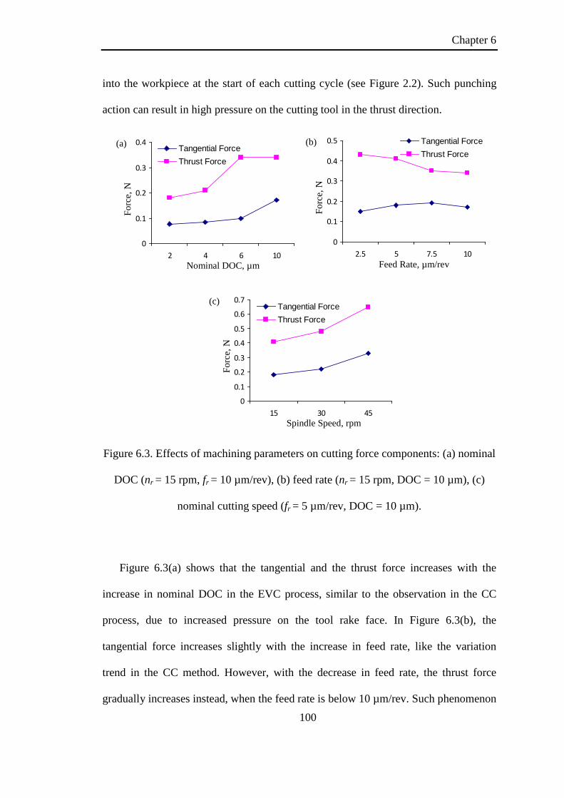
Chapter 6

100

into the workpiece at the start of each cutting cycle (see Figure 2.2). Such punching

action can result in high pressure on the cutting tool in the thrust direction.

Figure 6.3. Effects of machining parameters on cutting force components: (a) nominal


nominal cutting speed (fr = 5 µm/rev, DOC = 10 µm).

Figure 6.3(a) shows that the tangential and the thrust force increases with the

increase in nominal DOC in the EVC process, similar to the observation in the CC

process, due to increased pressure on the tool rake face. In Figure 6.3(b), the

tangential force increases slightly with the increase in feed rate, like the variation

trend in the CC method. However, with the decrease in feed rate, the thrust force

gradually increases instead, when the feed rate is below 10 µm/rev. Such phenomenon

(b)

0

0.1

0.2

0.3

0.4

0.5

2.5 5 7.5 10

Tangential ForceThrust Force

Feed Rate, µm/rev

Forc

e, N

(a)

0

0.1

0.2

0.3

0.4

2 4 6 10


Nominal DOC, µm

Forc

e, N

(c)

0

0.1

0.2

0.3

0.4

0.5

0.6

0.7

15 30 45


Spindle Speed, rpm

Forc

e, N

Chapter 6

101

is deemed to be caused by the decrease in uncut chip thickness induced by the

decrement in feed rate. Due to the small uncut chip thickness, the highly negative

effective rake angle, rather than the nominal rake angle tends to determine the

resulting force at these smaller feed rates. Hence, more significant ploughing action

can be caused by the highly negative effective rake angle which is induced by smaller

uncut chip thickness, as demonstrated by previous researchers (Lucca et al., 1993). It

can also be noticed in Figure 6.3(c) that both the tangential and the thrust force

components decrease with the decrease in spindle speed (or nominal cutting speed).

Such results correspond well with those found in the low-frequency EVC tests, as

shown in Figure 3.9.

6.2.2 Effects of cutting parameters on tool wear

Tool wear has strong influence on surface finish and dimensional accuracy of a

machined workpiece, and is also directly related to the machining cost and efficiency.

The photographs of flank faces of the PCD tools, and their close-up views were

captured by the Nomarski microscope. Figure 6.4 shows five selected photographs to

observe the effects of different nominal rotational speeds (see Figure 6.4(a)-(c)),

nominal DOCs (see Figure 6.4(c)-(d)) and feed rates (see Figure 6.4(d)-(e)). The

cutting length which varies with different feed rates for the five conditions can be

found in Table 6.2. It can be observed that the flank wear of almost all the used PCD

tools against the machining parameters is insignificant (less than 8 µm), except the

one with the higher spindle speed (45 rpm), as shown in Figure 6.4(a). Its flank wear

width is found to be about 14 µm at 110 m cutting length. Figure 6.4(b)-(e) show the

flank faces of two PCD tools under four different cutting conditions with two

relatively lower spindle speeds (30 rpm and 15 rpm), and their tool flank wear is

Chapter 6

102

much smaller than that in Figure 6.4(a). Hence it can be remarked that different

machining parameters, except the nominal cutting speed, do not have strong influence

on tool wear when machining hardened steel using PCD tools, and the PCD tool life

will become shorter with the increase in nominal cutting speed or speed ratio. The

main reason lies in that the higher speed ratio induces relatively larger portion where

the tool is in contact with the workpiece in each cutting cycle. The higher the speed

ratio, the more similar the EVC process is to the CC process, making the degree of

tool wear suppression in EVC weakened.

(a)

(b)

(c)

100 µm 20 µm

100 µm 20 µm

Feed direction

100 µm 20 µm

Chapter 6

103

(d)

(e)

Figure 6.4. Microscope (100× and 500 ×) photographs of the flank wear of PCD tools:

(a) DOC = 10 µm, fr = 5 µm/rev, nr = 45 rpm, Lc= 110 m, (b) DOC = 10 µm, fr = 5

µm/rev, nr = 30 rpm, Lc= 110 m, (c) DOC = 4 µm, fr = 10 µm/rev, nr = 15 rpm, Lc= 55

m, (d) DOC = 10 µm, fr = 10 µm/rev, nr = 15 rpm, Lc= 55 m, (e) DOC = 10 µm, fr =

7.5 µm/rev, nr = 15 rpm, Lc= 73 m.

6.2.3 Effects of cutting parameters on chip formation

The chips generated with the EVC method using PCD tools are collected and

analyzed by using the SEM. Four photographs of these chips observed at various

cutting conditions are shown in Figure 6.5. It can be seen that the chip thickness is

observed to be constant in each cutting condition. Furthermore, the formed chips are

found to be continuous in most of the cases (see Figure 6.5(b)-(d)), meaning that

continuous chip formation process is achieved with the spindle speed of 15 rpm and

30 rpm, while the chips with the 45 rpm spindle speed are non-continuous. The reason

for this phenomenon may lie in that the higher nominal cutting speed or speed ratio in

100 µm 20 µm

20 µm 100 µm

Chapter 6

104

the EVC method results in the larger cutting force (see Figure 6.3(c)) and the faster

tool wear (see Figure 6.4(a)), which can consequently induce less stable cutting

process and hence more breakable chips.

It is also interesting to find from Figure 6.5(a)-(c) that the chip width increases

with the increase in nominal cutting speed or speed ratio. Two reasons can be realized

with this observation. One reason is that the chip formation process may be affected

by the larger cutting force (see Figure 6.3(c)) resulting from the higher nominal

cutting speed. The larger cutting force may cause more significant lateral side flow of

material, which can consequently increase the width of chip. Another reason is that, as

stated in Chapter 3, transient TOC is increased with the increment of speed ratio (see

Figure 3.10), which may lead to a comparatively larger chip size.

(a) (b)

(c) (d)

Figure 6.5. SEM (250×) photographs of the curled chips with four different cutting

conditions in the EVC test (DOC=10 µm): (a) nr = 45 rpm, fr = 5 µm/rev, (b) nr = 30

rpm, fr = 5 µm/rev, (c) nr = 15 rpm, fr = 5 µm/rev, (d) nr = 15 rpm, fr = 7.5 µm/rev.

Chapter 6

105

6.2.4 Effects of cutting parameters on surface roughness

The surface roughness has a very important role in the production of precision

molds, and the fatigue and corrosion resistance of a mold can be significantly

enhanced by improving the surface quality. In this experimental test, the surface

profile is generated by feed marks along the feed direction due to the round tool nose,

and vibration marks along the nominal cutting direction due to the elliptical vibration

locus. The theoretical surface roughness caused by the feed marks is determined by

the tool nose radius rn and the feed rate fr. As the total theoretical surface roughness of

the machined surface with the EVC method is a superposition of the roughness caused

by the vibration marks and the roughness caused by the feed marks, its value is

determined not only by rn and fr, but also by the vibration parameters (a, b, ω and φ ),

the nominal cutting speed (vc) and the tool edge radius (re).

Figure 6.6 shows effects of different nominal DOCs, feed rates and spindle speeds,

on the average and maximum surface roughness values, Ra and Rz, respectively. In

examining Figure 6.6(a), it is observed that both Ra and Rz at 6 µm nominal DOC are

found to be lower than those at the higher nominal DOC of 10 µm. However, at the

nominal DOCs of 4 and 2 µm, which are equal to and less than the peak-to-peak

vibration amplitude, respectively, the surface roughness values are relatively larger

than the nominal DOC of 6 µm. It may be because that a smaller nominal DOC leads

to a smaller uncut chip thickness, which can cause more significant ploughing and

rubbing actions between the round tool edge and the material. Such actions can

consequently deteriorate the stable plastic deformation of material, which may

eventually increase the surface roughness.

Chapter 6

106

Figure 6.6. Effects of machining parameters on surface roughness values: (a) nominal


spindle speed (fr = 5 µm/rev, DOC = 10 µm).

In Figure 6.6(b), it is observed that Ra increases with the increase in feed rate, due

to that a smaller feed rate leads to a smaller surface roughness caused by the feed

marks. Though, Shamoto et al. have observed that the maximum surface roughness

converges to a certain value as the feed rate is reduced to less than 10 µm/rev when

applying the EVC method on hardened steel using SCD tools (Shamoto and Moriwaki,

1999). With ultraprecision machine tool used in the current test, the results in Figure

6.6(b) reveal that the surface finish can still be significantly improved using the PCD

tools at the feed rates less than 10 µm/rev.

(b)

0

0.05

0.1

0.15

0.2

0.25

2.5 5 7.5 10

RaRz

Feed Rate, µm/rev

Rou

ghne

ss, µ

m

(a)

0

0.05

0.1

0.15

0.2

0.25

0.3

2 4 6 10

RaRz

Nominal DOC, µm

Rou

ghne

ss, µ

m

(c)

0

0.05

0.1

0.15

0.2

0.25

15 30 45

RaRz

Spindle Speed, rpm

Rou

ghne

ss, µ

m

Chapter 6

107

Figure 6.6(c) shows the surface roughness values versus three different spindle

speeds. It can be observed that the surface roughness value at 45 rpm spindle speed is

much higher than those values at the other two relatively lower spindle speeds. One

reason for such phenomenon lie in the quick tool wear observed at a higher spindle

speed. In the previous section, on the analysis of tool wear, it has been stated that the

tool wear of PCD tools when machining hardened steel with the EVC method is

highly affected by nominal cutting speed, and the experimental results have shown

that the tool wear at 45 rpm spindle speed is much more significant than that at

smaller spindle speeds (see Figure 6.4). Such faster tool wear may significantly

increase the surface roughness value by inducing more ploughing mechanism in the

cutting process. Another reason lies in the increased height of vibration marks with

the increment of speed ratio, as shown in Figure 5.3 and Figure 5.12. Photographs of

the machined surfaces obtained with these spindle speeds are also captured by the

microscope, which are shown in Figure 6.7. It can be observed that with the increase

in spindle speed or nominal cutting speed, the vibration marks along the nominal

cutting direction are found to be more obvious.

Chapter 6

108

Figure 6.7. Microscope photographs (500×) of the machined surfaces at three

different spindle speeds (DOC = 10 µm, fr = 5 µm/rev): (a) nr = 15 rpm, (b) nr = 30

rpm, (c) nr = 45 rpm.

Figure 6.8(a) shows AFM scan of a square area of the machined surface with 45

rpm spindle speed and Figure 6.8(b)-(c) highlight the surface profiles along the feed

and the nominal cutting direction, respectively. As it can be observed from Figure

6.8(a) and (c), the vibration marks along the nominal cutting direction are obvious and

hence responsible as an important part for the surface roughness. It can also be seen

that the feature height in Figure 6.8(b) caused by the round nose is much larger than

the cusp height in Figure 6.8(c) resulting from the vibration marks. It means that the

feed marks contribute a larger part to the overall surface roughness of the machined

surface compared with the vibration marks. Furthermore, small chips and protrusions

are found to get adhered to the machined surface, which are difficult to clean up, as

seen in Figure 6.8(a). It might be caused by the high cutting force values (see Figure

6.3(c)), the fastest tool wear (see Figure 6.4(a)) and the non-continuous chips (see

Figure 6.5(a)) at the higher spindle speed (45 rpm) and accordingly the higher

nominal cutting speed.

Cutting direction Feed direction

(a) (b) (c)

Vibration marks

Chapter 6

109

Figure 6.8. AFM scan of the machined surface in the EVC test (DOC = 10 µm, fr = 5

µm/rev, nr = 45 rpm): (a) overview surface profile (90 µm × 90 µm), (b) measured in

the feed direction, (c) measured in the nominal cutting direction.

6.2.5 Evaluation test for obtaining mirror quality surface

Obtaining a mirror surface on hardened steel for die and using inexpensive PCD

tools instead of SCD tools is the ultimate concern of this study. In order to evaluate

the capability of PCD tools for this with the EVC method, an evaluation test is

conducted on the entire workpiece face area (40 mm diameter, 1257 mm2 area ) with

10 µm nominal DOC, 2.5 µm/rev feed rate and 15 rpm spindle speed. Such cutting

process with the combination of EVC and face turning results in a continually varying

nominal cutting speed varies from a higher value at a larger radius to a smaller value

towards the center of the workpiece. Figure 6.9 shows the picture of the machined

workpiece surface which is reflecting the word “NUS” representing “National

University of Singapore”. It can be observed that the inner circular zone

(approximately 806 mm2) can clearly reflect “NUS” and is considered as a mirror-like

surface, while the outer annular surface is a little blurred and cannot give a clear

reflection of “NUS”.

(c)

(b)

Feed Direction

Cutting Direction

(a)

9

Chapter 6

110

Figure 6.9. Machined surface on hardened stainless steel using a PCD tool with the

EVC technology (DOC = 10 µm, fr = 2.5 µm/rev, nr = 15 rpm).

The average surface roughness of the machined surface Ra measured by the stylus

profilometer is about 8 nm. The surface roughness at different radial locations is also

measured by the Zygo white light interferometer, as shown in Figure 6.10. The results

show that the whole machined surface can be apparently divided into two zones, the

inner circular zone and the outer annular zone, in terms of surface roughness values.

For the outer annular zone, where the radial distance is larger than 16 mm, the mean

value of measured Ra was found to be about 30 nm. However, when the radial

distance is less than 16 mm, Ra starts showing little variation with the change of radial

distance, and the Ra value in the inner circular area (about 804 mm2, obtained from

π×162) is measured to be about 11 nm. The reason for this phenomenon may line in

that the variation of tool-workpiece stiffness when the tool edge gets worn

progressively. When the fresh tool with a very sharp tool edge is used to machine the

workpiece, the contact area between tool edge and workpiece is too small to resist

chatter vibration, resulting in higher surface roughness and worse surface quality.

Chapter 6

111

After the tool edge is worn a little, the strength of the tool edge becomes higher, and

the contact area between tool edge and workpiece is larger. Then, chatter vibration

will be suppressed and better and stable surface quality can be obtained in a long

period until the tool is significantly worn.

Figure 6.10. Measurement results of surface roughness for the machinined surface.

Figure 6.11 shows the photographs of the tool flank face captured by the

microscope. It can be seen that the tool flank wear width is still not significant after

machining such hardened stainless steel for a surface area of 1257 mm2 with a cutting

length of 533.3 m. Such machining area is considered enough for die and molding

applications in the manufacturing industry. Therefore, it can be said that the PCD tool

with the EVC technology is capable for long-distance machining to achieve mirror-

like surface on hardened steel, if the cutting parameters are carefully controlled.

OD=40 mm

Ra=30 nm Ra=11 nm

Measurement windows

4 mm

Chapter 6

112

100 µm 20 µm

Figure 6.11. Microscope photographs (100× and 500 ×) of the worn PCD tool after

the evaluation EVC test on the hardened steel (DOC = 10 µm, fr = 2.5 µm/rev, nr = 15

rpm).


In this chapter, an experimental study on machining a hardened stainless steel

(Stavax, 49 HRC) using commercial PCD tools under the EVC method is carried out

to understand the effects of conventional machining parameters on different output

performance such as cutting force, tool flank wear, chip formation, and surface

roughness. Then, a separate test of machining about 1257 mm2 surface area on the

hardened steel is also carried out to investigate the capability of PCD tools for

obtaining mirror quality surface, as a demand of mold manufacturing industries.

Based on the experimental findings, conclusions can be compiled as follows:

• The two cutting force components (tangential and thrust force) increase with the

increment in nominal cutting speed. It is deemed to be caused by the decrement of

shear angle and the increment in transient TOC that are both induced by the

decrease in speed ratio.

• With the EVC method, the PCD tools used in cutting the hardened steel are able to

achieve better surface roughness at the nominal DOC of 6 µm as compared to

both the other higher and lower nominal DOCs.

Chapter 6

113

• The tool wear at lower spindle speeds (30 rpm and 15 rpm), after cutting the 550

mm2 surface area with the EVC method, is insignificant, while the tool wear at the

higher spindle speed (45 rpm) is found to be much larger (14 µm tool flank width).

• The higher spindle speed (45 rpm) results in more breakable chips than the other

tests with lower spindle speeds, most of which produce continuous chips with

constant chip thickness. The chip width increases with the increment of nominal

cutting speed.

• The experimental results show that nominal cutting speed (or spindle speed) has

strong influence on the surface roughness under the EVC method. The surface

roughness decreases with the decrement of feed rate and nominal cutting speed.

• The results of the separate evaluation test show that, for fabrication of die and

mold parts from hardened steels, mirror-like surface can be obtained by applying

the EVC method using the inexpensive PCD tools instead of the expensive SCD

tools.

Chapter 7

114

Chapter 7: Tool wear suppression mechanism

for machining steel using diamond with the

VAM method

As stated in Chapters 2 and 6, by employing VAM (i.e. CVC and EVC), diamond

tools can be used to cut steel sustainably, with significantly improved tool life

compared to CC (Moriwaki and Shamoto, 1991; Shamoto et al., 1999a). For the

reason of the reduced tool wear in VAM, most researchers attributed it to the

experimentally measured reduced cutting force, which they believe will lead to

smaller heat generation and reduced temperature in the VAM process (Brehl and Dow,

2008; Zhou et al., 2003). Such explanation seems to be reasonable because an

increased temperature usually leads to a higher chemical reaction rate and hence a

higher wear rate of diamond tools. However, in 2005, Mitrofanov et al. (Mitrofanov et

al., 2005b) found that the tool tip temperature in VAM is 15% higher than in CC by

monitoring the cutting process of machining Inconel 718 using carbide tools with the

infrared thermography. This experimental result is surprising and adverse to the other

researchers’ traditional speculation that VAM is supposed to produce smaller heat

generation and lower tool/workpiece temperature. Unfortunately, researchers did not

provide theoretical explanation and quantitative analysis for the observed

phenomenon, and no follow-up studies have been found to further verify and explain

their experimental results. Therefore, researchers are still confused about the extent of

Chapter 7

115

cutting energy consumption and tool/workpiece temperature in VAM, let alone their

role in slowing the tool wear. Moreover, as no theoretical and systematic explanations

have been made on the tool wear suppression of diamond in VAM of steel by

previous researchers, the inherent reasons are still unclear and needs in-depth studies

on this issue.

In this chapter, firstly, cutting energy consumption for VAM is quantitatively

modeled and calculated by investigating the transient cutting force and the

corresponding tool motion position. Secondly, workpiece temperatures are measured

in CC and VAM of steel by using a contacting thermocouple, and the obtained results

are compared and explained carefully. Finally, experimental tests are conducted to

investigate and compare the tool wear condition of PCD tools in CC and VAM of

carbon steel. Based on the comparison results and previous researchers’ relevant

studies, two main reasons, instead of the speculated reduced temperature, are

proposed and discussed for the reduced wear rate of diamond tools in VAM of steel.

7.1 Modeling of cutting energy consumption in VAM

Cutting energy is defined as the work done by the cutting tool in order to remove

workpiece materials, and is mainly spent in elastic and plastic deformation of

materials, and the friction on the tool rake and flank faces. Such mechanical energy

will be converted irreversibly into heat, which is eventually dissipated into the

ambient environments (e.g. tool, workpiece, air, etc.) and then leads to a higher

tool/workpiece temperature. It can be said that, under otherwise identical conditions,

the cutting energy is in direct proportion to the tool/workpiece temperature. Hence, in

the following part of this section, the cutting energy consumption in VAM is modeled

and calculated based on the transient cutting force for each cutting cycle.

Chapter 7

116

In order to obtain the transient cutting force in VAM, a series of low-frequency

orthogonal CVC and EVC (i.e. 1D and 2D VAM) tests with four different speed ratios

(0.025, 0.05, 0.075 and 0.1) are conducted on 6061 aluminum alloy workpiece. The

vibration loci can be generated according to Equations (2.1) and (2.9), and the

procedure for generating the vibration motion can be found in Chapter 3. The

transient cutting force for CC and EVC can be obtained from Chapters 3 and 4, and

the orthogonal CVC tests are conducted under the same cutting and vibration

conditions with the EVC tests as shown Table 3.1, except that the thrust amplitude b

is set zero.

Figure 7.1 shows the maximum resultant force Rmax against different speed ratios

for the three cutting methods (CC, CVC and EVC). As found by previous researchers,

it can be seen from Figure 7.1 that the maximum resultant force in VAM is smaller

than that in CC, and EVC produces even smaller force compared to CVC. In both the

CVC and EVC processes, the value of Rmax will decrease with the decrement of the

speed ratio Rs. Such phenomenon may be caused by the reduced value of transient

thickness of cut and the increased value of transient shear angle in each cutting cycle.

As an example, the recorded transient cutting force components (principal and thrust

force) for the three cutting methods (CC, CVC and EVC) at the cutting speed of 0.188

mm/min (i.e. Rs=0.1) are shown in Figure 7.2(a)-(c).

Chapter 7

117

0

2

4

6

8

0.025 0.05 0.075 0.1 CC

Speed ratio, R s

Max

imum

resu

ltant

forc

e, R

max

, (N

)

CC CVC EVC

Figure 7.1. Maximum resultant cutting force in the CC and VAM processes.

0 0.5 1 1.5 2 2.5 3

-1

0

1

2

3

4

5

6

7

Time, s

Cut

ting

forc

e, N

Principal force Thrust force

(a)

Chapter 7

118

Cut

ting

forc

e, N

0

-1

2

1

3

4

5 Thrust force Principal force

Phase of vibration, rad π/2 0 π 3π/2 2π

6

D'

F D

F'

(b)

Cut

ting

forc

e, N

0

-1

2

1

3

4

5

Phase of vibration, rad π/2 0 π 3π/2 2π

Principal force Thrust force

A B E

F

(c)

Figure 7.2. Experimental transient cutting force components in: (a) CC, (b) CVC, (c)

EVC.

Chapter 7

119

In the CC process (see Figure 7.2(a)), the principal force Fp is stable and can be

assumed to be constant, and the thrust force does not do work due to no relative

movement along the thrust direction. Hence, given a cutting distance of Lc, the total

work done by the cutting tool (i.e. cutting energy consumption) can be calculated as

follows:

pcCC FLW = (7.1)

Figure 7.2(b) shows the transient cutting force components in the CVC process,

where the points G and H correspond with the theoretical cutting-start and cutting-end

points, as shown in Figure 2.1. It can be seen that, before the tool edge arrives at point

G, the tool rake face has already contacted with the workpiece material. During the

elastic deformation process from the actual tool/workpiece engagement point G' to

point G, material stress is progressively increased and elastic energy is accumulated.

Then the workpiece material from point G to point H will be removed from the

workpiece by the cutting tool through plastic deformation. After that, the material will

experience an unloading and elastic recovery process, during which the material stress

will be released gradually until the elastic energy is fully dissipated at the actual

tool/workpiece disengagement point H'. Figure 7.3 schematically shows the CVC

process considering elastic deformation and recovery in a cutting cycle.

In the CVC process, the transient principal force Fp(t) varies over time in each

cutting cycle, while in the CC process, the transient thrust force Ft(t) does not do work

due to no thrust directional relative movement. Hence, it is not applicable to use

Equation (7.1) to calculate the cutting energy consumption in CVC. In such case, it is

necessary to divide the tool motion locus into small steps, and the work done by the

tool in a cutting cycle can be calculated as the sum over these small steps. Meanwhile,

Chapter 7

120

as the number of cutting cycles experienced for a given cutting distance of Lc can be

calculated as cc vfL / , the cutting energy consumption in CVC can be given by the

following equation:

∫=Ht

pc

cCVC dttxtFvfLW

0)(')( (7.2)

where ∫Ht

p dttxtF0

)(')( represents the work done by the cutting tool in a cutting cycle.

The value of Ht and )(' tx can be derived from Equations (2.3) and (2.7) in Chapter 2.

The upper limit of the integration is set as Ht , due to the fact that, after passing point

H, the tool will recede from the workpiece and stop doing positive work. In fact, in

the period from point H to point H', the elastic energy accumulated in the workpiece

material is dissipated gradually into the ambience, and no cutting energy is consumed

by the tool.

Chip Tool

Workpiece vc/f

H

G

H'

G'

Elastic deformation

Elastic recovery

x'(t)

Figure 7.3. Schematic illustration of the CVC process considering elastic deformation

and recovery.

Chapter 7

121

Figure 7.2(c) shows the transient cutting force components in the EVC process.

The points A, B, E and F correspond with the relevant points in Figure 2.2(a). Like

the CVC process, in EVC, elastic deformation and recovery will also happen due to

the periodical vibration along the nominal cutting direction. However, the work in

EVC is not only done by the principal force, but also by the thrust force, due to the

existence of relative movement along the thrust direction (see Figure 2.2(a)).

Furthermore, as the transient thrust force is not reversed in direction until arriving at

point E, its direction should be opposite to the thrust directional tool velocity during

the interval from point B to point E, where the transient thrust force does not do

positive work. Therefore, based on analyses of the motion locus and the variation of

transient cutting force, the cutting energy consumption in EVC can be calculated as

follows:

++= ∫∫∫

π2

00)(')()(')()(')(

E

BF

t t

t

t

t

pc

cEVC dttytFdttytFdttxtFvfLW (7.3)

where ∫Ft

p dttxtF0

)(')( is the work done by the transient principal force, and

∫∫ +π2

0)(')()(')(

E

B

t t

t

t dttytFdttytF represents the work done by the transient thrust

force. )(' tx and )(' ty represent the transient tool velocities along the x- and y- axes

(see Equation (2.10)), and Bt , Et and Ft represent the time when the tool passes the

points B, E and F, respectively. The values of Bt and Ft can be calculated from

Equations (2.16) and (2.13), and the value of Et can be found directly from the

experimental value of transient thrust force (see Figure 7.2(c)).

Based on the obtained values of transient cutting force, the cutting energy

consumption for the three cutting methods by the cutting tool can be calculated by

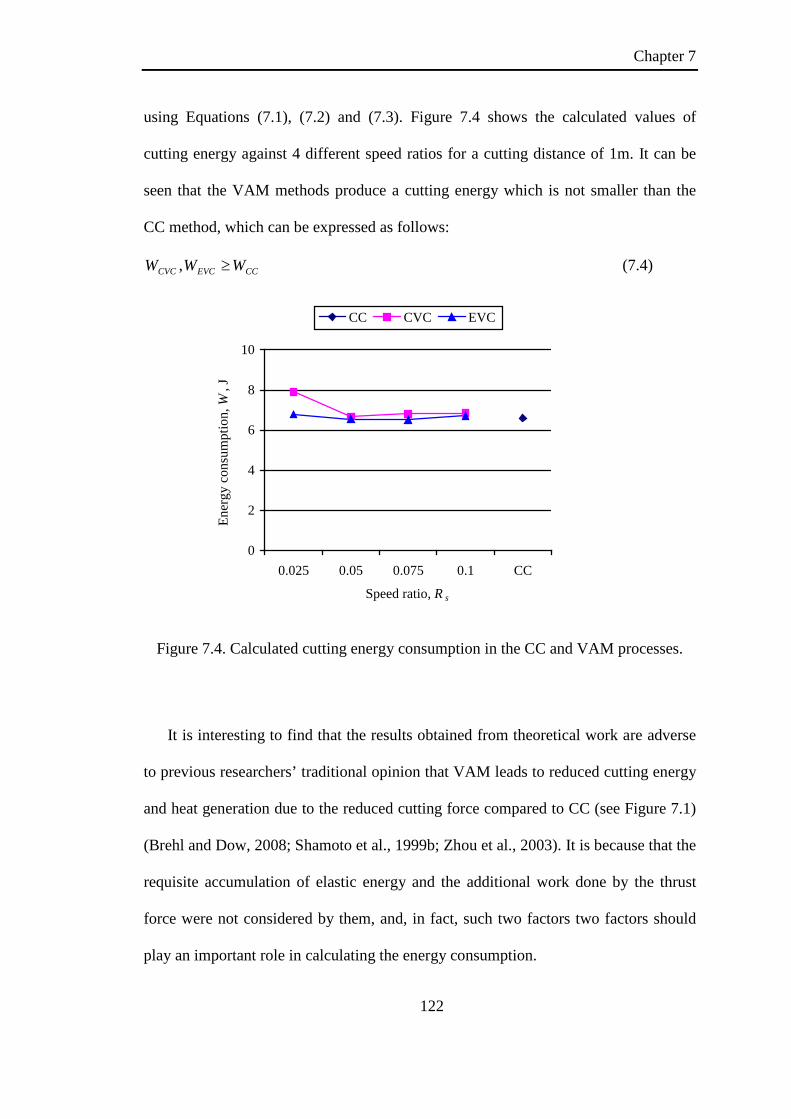
Chapter 7

122

using Equations (7.1), (7.2) and (7.3). Figure 7.4 shows the calculated values of

cutting energy against 4 different speed ratios for a cutting distance of 1m. It can be

seen that the VAM methods produce a cutting energy which is not smaller than the

CC method, which can be expressed as follows:

CCEVCCVC WWW ≥, (7.4)

0

2

4

6

8

10

0.025 0.05 0.075 0.1 CC

Speed ratio, R s

Ener

gy c

onsu

mpt

ion,

W, J

CC CVC EVC

Figure 7.4. Calculated cutting energy consumption in the CC and VAM processes.

It is interesting to find that the results obtained from theoretical work are adverse

to previous researchers’ traditional opinion that VAM leads to reduced cutting energy

and heat generation due to the reduced cutting force compared to CC (see Figure 7.1)

(Brehl and Dow, 2008; Shamoto et al., 1999b; Zhou et al., 2003). It is because that the

requisite accumulation of elastic energy and the additional work done by the thrust

force were not considered by them, and, in fact, such two factors two factors should

play an important role in calculating the energy consumption.

Chapter 7

123

From Figure 7.1, it can be observed that a smaller speed ratio leads to a smaller

cutting force. However, the value of cutting energy consumption for VAM varies in a

different way, which should be caused by the increased number of cutting cycles (i.e.

cc vfL / ) for a unit of cutting length resulted from a smaller speed ratio. In that case,

the material needs to experience more times of elastic deformation and hence

accumulate more elastic energy during the VAM process.

According to the directly proportional relationship between cutting energy

consumption and tool/workpiece temperature, it is highly possible that VAM may also

produce a workpiece temperature which is not smaller than CC. Therefore, in order to

verify the above theoretical proposal experimentally, the workpiece temperatures in

CC and VAM are measured in the next section.

7.2 Measurement of the workpiece temperature

The workpiece temperatures in the CC, CVC and EVC processes are measured by

a contacting thermocouple, which is placed close to the machined area. Figure 7.5(a)

and (b) show the schematic and physical illustration of the experimental setup, where

the workpiece is kept fixed on the vacuum chuck, and the cutting tool is moved by

driving the Y-axis of the ultraprecision machine tool. Three fresh PCD tools are used

to groove 6 times uninterruptedly on a workpiece made of carbon steel for the three

cutting methods, and the nominal depth of cut for every grooving is set at 10 µm. Due

to the gradually increasing groove width, the volume of removed material becomes

larger and larger with the increase of groove number (see Figure 7.5(a)). The

machined grooves are located 0.1 mm away from the center hole of the workpiece,

where the thermocouple junction is fixed. Meanwhile, a temperature data logger is

connected with the thermocouple to measure the junction temperature, which is then

Chapter 7

124

recorded in the computer. In the VAM process, the vibration of tool tip is generated

by several piezoelectric actuators stacked in a metal block. The vibrator vibrates at a

frequency of 38.87 kHz with a phase difference of 90o, and the tangential and thrust

vibration amplitudes (i.e. a and b) can be set by adjusting the controller of the VAM

device. Table 7.1 lists the detailed cutting and vibration conditions for measuring the

workpiece temperature.

Chapter 7

125

Groove

Insulation material

Workpiece

Thermocouple junction

Data logger

Computer

0.1 mm

6×10 µm

Heat

Groove No. 1

No. 6

(a)

VAM deviceThermocouple

Workpiece

PCD tool

GrooveThermocouple junction

Cutting direction

Y-axis

(b)

Figure 7.5. Illustration of the experimental setup for measuring the workpiece

temperature: (a) schematic view, (b) physical view.

Chapter 7

126

Table 7.1. Conditions for measurement of the workpiece temperature.

Workpiece material Carbon steel (ASSAB 760) Tool PCD tool (0.6 nose radius) Lubrication condition Dry cutting Nominal depth of cut, [µm] 6×10 Nominal cutting speed, vc [mm/min] 450

Vibration amplitudes, [µm] a=0, b=0 (CC)

a=2, b=0 (CVC)

a=2, b=2 (EVC)

Figure 7.6 shows results for the temperature variation measured in the

experimental tests. During the machining process, mechanical work is done by the

cutting tool as the workpiece material is removed. Meanwhile, the consumed cutting

energy is eventually converted into heat, which will be partially dissipated into the

workpiece material and raise the workpiece temperature. The workpiece temperature

will rise to a peak value once the tool passes the thermocouple junction. Then, due to

the dissipation of heat into the ambient environment, the workpiece temperature will

fall gradually. From Figure 7.6, it can be observed that the peak values of temperature

rise for both CVC and EVC are not smaller than that for CC, as expressed in the

following equation:

CCEVCCVC TTT ∆≥∆∆ , (7.5)

Hence, it is reasonable to expect that, for the same material removal rate, more heat is

transmitted from the tool/workpiece interface to the thermocouple junction, due to

more consumed cutting energy in the VAM process compared to CC. Such

experimental findings, together with the results obtained by Mitrofanov et al.

(Mitrofanov et al., 2005b), can verify that the proposed theory in the previous section

is reasonable and reliable.

Chapter 7

127

Figure 7.6. Temperature variation of the workpiece under different cutting methods.

Furthermore, from Figure 7.6, it is interesting to observe that the EVC produces

much larger temperature rise compared to the CVC, which does not comply well with

the theoretical analysis on cutting energy consumption (see Figure 7.4). The main

reason for this phenomenon may lie in that the edge radius of the PCD tool used in

grooving workpiece is significantly larger than that of the SCD tool used in obtaining

the transient cutting force. Due to the micron-level edge radius of the PCD tool, when

the tool edge moves from the cutting-start point A to the bottom point B (see Figure

2.2(a)), the tool edge will punch some material into the workpiece surface, and then

induce a much larger transient thrust force than expected. Hence, more cutting energy

will be consumed, and the workpiece temperature can be raised higher due to the

increased heat generation.

0 1 2 3 4 5 6 -0.2

+0

+0.2

+0.4

+0.6

+0.8

+1

Groove number

Tem

pera

ture

rise

, ΔT,

o C

CC CVC EVC

Chapter 7

128

In the previous two sections, the theoretical analysis and the experimental

investigation have demonstrated that VAM do not produce smaller cutting energy and

lower tool/workpiece temperature compared to CC. Furthermore, it has been found

that the wear rate of diamond tool in machining steel is not affected as the workpiece

temperature is artificially heated to 220 oC from 20 oC (Thornton and Wilks, 1979),

which implies that the graphitization rate is not thermally activated in such

temperature interval. Considering the extremely low cutting speed in VAM (Brehl and

Dow, 2008; Zhang et al., 2011), even based on a conservative estimate (Thornton and

Wilks, 1979), the flash temperature in the tool/workpiece interface should be less than

220 oC. Hence, it can be concluded that the reduced wear rate of diamond tools in

machining steel using VAM should not be caused by the reduced temperature claimed

by previous researchers.

7.3 Tool wear suppression mechanism in VAM

7.3.1 Experimental investigation

Before proposing reasons for the tool wear suppression mechanism in VAM, the

tool wear conditions for the CC, CVC and EVC methods are experimentally

investigated when machining steel using PCD tools. In the cutting tests, face turning

is conducted on a circular flat surface with a diameter of 18 mm by using a fresh PCD

tool, which is mounted on the VAM device, as shown Figure 7.7. The cutting tool is

fed from the outer edge of the workpiece to the center, and the cutting distance is

calculated to be about 102 m. Meanwhile, the wear conditions of the three PCD tools

with the three cutting methods (CC, CVC and EVC) are experimentally investigated

by using a microscope (OLYMPUS STM 6) to capture photographs of the tool flank

Chapter 7

129

faces. Table 7.2 shows the detailed cutting and vibration conditions for the

experimental tests.

Figure 7.7. Experimental setup for machining steel using PCD tools.

Table 7.2. Conditions for machining steel using PCD tools with CC and VAM

methods.

Workpiece material Carbon steel (ASSAB 760) Tool PCD tool (0.6 nose radius) Lubrication condition Air cooling Depth of cut, [µm] 10 Feed rate, [µm/rev] 2.5 Rotational speed, [rpm] 20 Nominal cutting speed, [mm/min] 0 ~ 1.131×103

Vibration amplitudes, [µm] a=0, b=0 (CC)

a=2, b=0 (CVC)

a=2, b=2 (EVC)

Figure 7.8 shows the microscope photographs of the tool flank faces for the three

PCD tools after the face turning tests. It can be observed that the VAM methods

produce significantly smaller tool wear compared to the CC method. For CVC (see

Figure 7.8(b)), only slight tool flank wear exists around the tool edge, while for EVC

(see Figure 7.8(c)), the tool wear is hardly able to detect. Such comparison results also

correspond well with previous researchers’ experimental studies on tool wear in

machining steel using diamond tools (Moriwaki and Shamoto, 1991; Shamoto and

Chapter 7

130

Moriwaki, 1999; Zhou et al., 2003). Since it has been verified that the claimed

reduced temperature does not contribute as a reason for such phenomenon, it is

necessary to find other reasonable explanations for the reduced wear rate. Hence, in

the following part of this section, based on previous researchers’ studies and the

experimental results in this study, two reasons are proposed for the reduced wear rate

of diamond in VAM of steel.

Chapter 7

131

X450 X1000

(a)

(b)

(c)

Figure 7.8. Microscope photographs of the tool flank faces in the three machining

processes: (a) CC, (b) CVC, (c) EVC.

100 µm 50 µm

50 µm 100 µm

100 µm 50 µm

Feed direction

Chapter 7

132

7.3.2 Contamination of the tool-workpiece interface

In order to understand the inherent reason for the high chemical wear rate of

diamond in machining steel, Thornton and Wilks conducted an extensive number of

experiments to investigate the effects of air pressure, cutting speed and temperature

on the tool wear condition of diamond in machining steel (Thornton and Wilks, 1979).

Based on the obtained experimental results, they have concluded that the quick wear

of diamond tool should be caused by the freshly machined steel surfaces generated

during machining, which have an enhanced chemical activity and strong chemical

affinity with diamond. Table 7.3 shows the wear rates of diamond tools in machining

mild steel at a cutting speed of 0.16 m/s under different atmosphere. The wear rate is

defined as the ratio between the area of wear flat on tool flank face and the machined

area of metal material, which is quoted in the unit of 10-6 (mm2mm-2). It can be seen

from Table 7.3 that the wear rates in near-vacuum condition (10-4 atm) are

significantly larger than those in Argon with normal pressure (1 atm). As Argon is

inert and forms no confirmed stable compounds under most conditions, Thornton and

Wilks attributed the reduced tool wear in Argon to the contamination of

tool/workpiece interface by the gaseous atmosphere, which can penetrate into the

interface and block off the chemical reaction and the catalyzed graphitization of

diamond.

Table 7.3. Wear rates of diamond tools for turning mild steel using CC method (10-6

mm2mm-2) (Thornton and Wilks, 1979).

Diamond Tool 10-4 atm 1 atm (Argon) 1 atm (Air) DS11R 14 2 0 DS13R 12 5 3 DS14R 8 0 0

Chapter 7

133

In the VAM process, the tool rake face contacts and separates from the workpiece

material regularly, and the tool/workpiece interface is exposed to the ambient

atmosphere periodically, as shown in Figure 7.9(a), while in the CC process, the tool

edge is pressed into contact with the freshly machined steel surface, and the wear flat

on the tool flank face is almost sealed off from the surrounding atmosphere by the

presence of freshly machined surface, as shown in Figure 7.9(b). Only limited

gaseous atmosphere can penetrate into the tool/workpiece interface to block the

chemical reaction in CC, but the intermittent cutting process in VAM will allow much

more air to penetrate into the tool/workpiece interface, and strongly enhance the

extent of contamination. Hence, the chemical reaction between diamond tool and the

freshly machined steel surface can be blocked off more effectively compared to CC.

Compared to CVC, in EVC process, both the rake face and the flank face will

separate from the workpiece periodically (see Figure 2.2). Such characteristics will

allow more gaseous atmosphere to penetrate into the tool/workpiece interface, which

may further enhance the degree of contamination and block off the graphitization.

Moreover, the contacting time between the tool flank face and the workpiece is

reduced in EVC, which can decrease the chemical reaction time and hence the tool

wear rate.

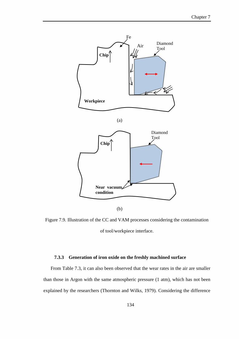
Chapter 7

134

(a)

(b)

Figure 7.9. Illustration of the CC and VAM processes considering the contamination

of tool/workpiece interface.

7.3.3 Generation of iron oxide on the freshly machined surface

From Table 7.3, it can also been observed that the wear rates in the air are smaller

than those in Argon with the same atmospheric pressure (1 atm), which has not been

explained by the researchers (Thornton and Wilks, 1979). Considering the difference

Chip

Workpiece

Fe Diamond Tool Air

Chip

Diamond Tool

Near vacuum condition

Chapter 7

135

between air and Argon, this phenomenon is probably caused by the existence of active

oxygen in the air, which may react with the freshly machined steel surface to form a

very thin (in nanoscale) layer of iron oxide (FexO) (Komanduri and Shaw, 1976).

However, it is the free iron atoms that act as a metal catalyst in both graphitization

and diamond nucleation. The iron oxide, which is relatively inert, does not act as a

metal catalyst in the transformation between diamond and graphite. Moreover, the

physical layer of iron oxide will even block the chemical reaction between free iron

and carbon atoms (Qin et al., 2006), and hence suppress the graphitization.

Figure 7.10 shows a schematic view of the VAM process considering the

generation of iron oxide. In CC process, as the tool/workpiece interface is not exposed

to the air atmosphere periodically (see Figure 7.9(b)), the generation of iron oxide on

the freshly cut surface is limited, while in VAM process, the air with oxygen will

penetrate into the tool/workpiece interface and react with the freshly machined steel

surface to form a thin layer of iron oxide. Due to the inertness of the iron oxide (Qin

et al., 2006), the graphitization process of diamond will be blocked until the tool edge

breaks the oxide layer (see Figure 7.10(b)).

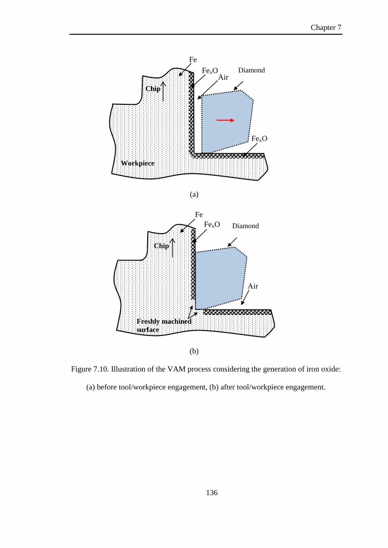
Chapter 7

136

(a)

(b)

Figure 7.10. Illustration of the VAM process considering the generation of iron oxide:

(a) before tool/workpiece engagement, (b) after tool/workpiece engagement.

Chip

Workpiece

Fe Diamond

FexO Air

FexO

Fe

Chip

FexO

Air

Diamond

Freshly machined surface

Chapter 7

137

(a)

0

0.5

1

1.5

2

2.5

3

3.5

CC CVC EVC

Cutting method

Oxy

gen

mas

s, %

(b)

Figure 7.11. EDS analysis of the tool flank faces for the used PCD tools: (a) EDS spectrums

for the tool used in EVC, (b) Comparison of oxygen mass for the three cutting

methods.

KeV

Cou

nts

Chapter 7

138

Energy-dispersive X-ray spectroscopy (EDS) analysis is also conducted on the

worn area on the tool flank faces of the three used PCD tools (see Figure 7.8) after

machining steel, and the mass of oxygen is analyzed during the analysis. Figure 7.11

shows results of the EDS analysis for the used PCD tools. It can be seen that the mass

of oxygen is almost zero for the CC process, and the VAM methods produces much

higher oxygen mass. It can be speculated that the oxygen exists as a form of iron

oxide, and such iron oxide on the tool flank face is accumulated gradually when the

tool edge is cutting or rubbing on the workpiece material. Hence, it is reasonable to

conclude that little iron oxide is generated during the CC process, and much more iron

oxide is formed in the VAM process. Such observation complies well with the above

proposed reason that VAM can strengthen the generation of iron oxide to block the

chemical reaction between the diamond and the freshly cut steel surface.


In this chapter, in order to strengthen the understanding of tool wear mechanism

of diamond in machining steel using VAM methods, both theoretical and

experimental investigation has been conducted. Based on the results, conclusions can

be compiled as follows:

• Based on the obtained transient cutting force in VAM, the cutting energy

consumption is theoretically modeled, and the results show that VAM does not

produce smaller cutting energy or heat generation compared to CC.

Chapter 7

139

• It is found that the workpiece temperature in VAM is not smaller than that in the

CC process, corresponding with the theoretical work about the cutting energy

consumption.

• Both 1D and 2D VAM do not produce lower cutting energy or lower workpiece

temperature than CC. Hence, the reduced tool wear of diamond in machining

steel with VAM is not caused by the speculatively lower tool/workpiece

temperature and heat generation which is claimed by the prevailing theory.

• CC produces significantly larger tool wear than VAM, and EVC produces the

smallest tool wear among the three methods.

• Based on the understandings of previous researchers’ studies on the chemical

wear of diamond tool, two main reasons are proposed for the significantly

reduced wear rate of diamond in VAM of steel: i) contamination of the

tool/workpiece interface, and ii) generation of iron oxide.

Chapter 8

140

Chapter 8: Main conclusions and

recommendations

8.1 Main contributions

In this study, cutting force, surface generation and tool wear mechanism for the

EVC method are studied experimentally and analytically. The main contributions of

this study are summarized as follows:

1. Experimental investigation and modeling of transient cutting force in the

EVC process

• In order to investigate the transient cutting force in EVC, a novel method is

proposed to realize the low-frequency EVC motion by conducting G-code

programming and axis motion control of an ultraprecision machine tool. The

effects of three essential cutting and vibration parameters (speed ratio, tangential

and thrust amplitude) are experimentally investigated and explained through

analyzing the transient TOC and the friction reversal time. Mathematical

evaluation of the transient TOC reveals that its value varies significantly in each

EVC cycle and hence is necessary to be considered in the force model.

• An analytical force model for orthogonal EVC process is developed for in-depth

understanding of the transient cutting mechanism and for accurate prediction of

the transient cutting force components. Based on the variation of friction modes,

each cutting cycle is divided into three consecutive zones: CC-like kinetic-friction

zone, static-friction zone and reverse kinetic-friction zone. A calculation method

Chapter 8

141

of the transient shear angles for the three zones is derived by investigating the

transient tool/chip velocities and employing Lee and Shaffer’s slip-line solution.

• The predicted transient force values based on the proposed analytical force model

are found to be in good agreement with the experimental results of the orthogonal

EVC tests. Hence, the proposed model can finely express the EVC mechanism

and assist to predict more accurate cutting force values compared to the earlier

model.

2. Modeling the effect of tool edge radius on surface generation in the EVC

process.

• An experimental study comprising a series of grooving tests using an SCD tool is

firstly carried out to clearly understand the surface generation along nominal

cutting direction in the EVC process, and the experimental roughness values are

compared with the theoretical ones based on previous researchers’ calculation

method.

• Based on the geometrical analysis for EVC surface generation process, effects of

the round tool edge on material removal mechanism are investigated, and a

comprehensive calculation method for determining the theoretical surface

roughness considering the edge radius is developed. Simulation results based on

the proposed model show that the theoretical roughness decreases with the

increment of tool edge radius.

• According to experimental results of a series of grooving tests using a PCD tool

with the EVC method, it is shown that the proposed model could predict much

more accurate surface roughness than the prevailing model, in which the tool edge

Chapter 8

142

radius is not considered. This analytical surface generation model should be

helpful for the performance evaluation and further application of the EVC method.

3. Experimental study on hardened steel using PCD tools with the EVC method.

• An experimental study on machining hardened stainless steel (Stavax, 49 HRC)

using commercial PCD tools under the ultrasonic EVC method is carried out to

understand the effects of conventional machining parameters on different output

parameters such as cutting force, tool flank wear, chip formation, and surface

roughness.

• The experimental results also show that nominal cutting speed has strong

influence on the surface roughness with the ultrasonic EVC method. It is also

found that the wear of the PCD tools at lower spindle speeds is insignificant and

not easy to detect, and the tool wear at the higher spindle speed is much larger.

• A separate test of machining about 1257 mm2 surface area on the hardened steel is

carried out to realize the capability of PCD tools for obtaining mirror quality

surface, as a demand for die and mold manufacturing industries. The results of the

separate evaluation test show that, for the fabrication of die and mold parts from

hardened steels, mirror-like surface can be obtained using inexpensive PCD tools

instead of highly-expensive SCD tools. This study may help industry increase the

efficiency and lower the manufacturing cost with the EVC method.

4. In-depth study on the tool wear suppression mechanism for machining steel

using diamond with the VAM method.

• Based on the obtained transient cutting force in VAM, cutting energy

consumption in the VAM process is theoretically modeled, and workpiece

Chapter 8

143

temperatures in the CC and VAM processes are experimentally measured by a

contacting thermocouple.

• Both the theoretical and experimental comparison results lead to a fact that VAM

does not produce smaller cutting energy and heat generation compared to CC. It

can be concluded that the reduced tool wear of diamond in VAM of steel is not

caused by the reduced heat generation and tool/workpiece temperature claimed by

previous researchers.

• Finally, two main reasons are proposed for the significantly reduced wear rate of

diamond in VAM of steel: i) contamination of the tool/workpiece interface, and ii)

generation of iron oxide. This study could provide better understandings of

diamond tool wear mechanism and hence is useful for researchers to develop other

new effective methods to suppress the fast chemical wear rate.

8.2 Recommendations for future work

1. Although the proposed analytical force model has provided a quick method to

calculate the transient cutting force, it still can be further improved. For example,

the elastic deformation of workpiece or chip material in a vibration cutting cycle

can be considered to understand the material deformation process. More important,

the shear stress is assumed to be constant in the proposed model, but its actual

value may change with the variation of cutting parameters. Furthermore, in order

to apply the force model in predicting the cutting force in VAM of brittle

materials, more factors need to be considered, such as tool edge radius and

specific cutting energy.

Chapter 8

144

2. The surface profile generated by elliptical-vibration assisted turning includes feed

marks along the feed direction and the vibration marks along the nominal cutting

direction. In this study, the proposed surface generation model only predicts the

roughness along the nominal cutting direction. In order to better understand micro

structures of the whole surface profile and predict its surface roughness values, a

more comprehensive model needs to develop to provide more guidance and

broaden the application of EVC method.

3. Researchers have already demonstrated that diamond tools with the (1 1 0) plane

as the rake face perform better than the conventional diamond tools with the (1 0 0)

plane as the rake face, in terms of tool wear and surface roughness. It is suggested

that these specialized tools can be applied in ultrasonic vibration cutting of hard

and brittle materials (such as hardened steel tungsten carbide, glass and ceramics)

to further suppress the tool wear.

4. Although the two reasonable reasons are proposed for diamond tool wear

suppression mechanism in VAM of steel in this study, they still need to be proven

by further experimental and theoretical investigation. Moreover, based on the

proposed theory, other novel methods can be proposed to effectively suppress the

chemical wear of diamond tools in machining steel. For example, to prevent the

chemical reaction between diamond and active iron atoms, iron oxide can be

generated on the steel surface by chemical treatment before cutting with diamond

tools; air cooling with more oxygen than normal air can be applied to assist to

Chapter 8

145

accelerate the generation of iron oxide to further suppress iron-catalyzed diamond

tool wear.

References

146

References

Ahmed, N., Mitrofanov, A.V., Babitsky, V.I., Silberschmidt, V.V., 2006. Analysis of

material response to ultrasonic vibration loading in turning Inconel 718. Mater. Sci.

Eng., A 424, 318-325.

Ahmed, N., Mitrofanov, A.V., Babitsky, V.I., Silberschmidt, V.V., 2007a. 3D finite

element analysis of ultrasonically assisted turning. Comput. Mater. Sci. 39, 149-154.

Ahmed, N., Mitrofanov, A.V., Babitsky, V.I., Silberschmidt, V.V., 2007b. Analysis of

forces in ultrasonically assisted turning. J. Sound Vib. 308, 845-854.

Ahn, J.H., Lim, H.S., Son, S.M., 1999. Improvement of micro-machining accuracy by

two-dimensional vibration cutting, ASPE, pp. 150-153.

Amini, S., Shamoto, E., Suzuki, N., Nategh, M.J., 2010. FE analysis of one-

directional and elliptical vibration cutting processes. Int. J. Aut. Technol. 4, 252-258.

Astashev, V.K., Babitsky, V.I., 1998. Ultrasonic cutting as a nonlinear (vibro-impact)

process. Ultrason. 36, 89-96.

Babitsky, V.I., Astashev, V.K., Kalashnikov, A.N., 2004a. Autoresonant control of

nonlinear mode in ultrasonic transducer for machining applications. Ultrason. 42, 29-

35.

Babitsky, V.I., Mitrofanov, A.V., Silberschmidt, V.V., 2004b. Ultrasonically assisted

turning of aviation materials: Simulations and experimental study. Ultrason. 42, 81-86.

Brehl, D.E., Dow, T.A., 2008. Review of vibration-assisted machining. Precis. Eng.

32, 153-172.

References

147

Brinksmeier, E., Glabe, R., 1999. Elliptical vibration cutting of steel with diamond

tools, ASPE, USA, pp. 163-166.

Casstevens, J.M., 1983. Diamond turning of steel in carbon-saturated atmospheres.

Precis. Eng. 5, 9-15.

Evans, C., Bryan, J.B., 1991. Cryogenic diamond turning of stainless steel. CIRP Ann.

40, 571-575.

Ikawa, N., Tanaka, T., 1971. Thermal aspects of wear of diamond grain in grinding.

CIRP Ann. 19, 153-157.

Isaev, A., Anokhin, V., 1961. Ultrasonic vibration of a metal cutting tool. Vest

Mashinos 41.

Komanduri, R., Shaw, M.C., 1976. On the diffusion wear of diamond in grinding pure

iron. Philosophical Magazine 34, 195-204.

Kumabe, J., Fuchizawa, K., Soutome, T., Nishimoto, Y., 1989. Ultrasonic

superposition vibration cutting of ceramics. Precis. Eng. 11, 71-77.

Kumbabe, J., 1979. Vibratory cutting. Jikkyou Publishing Co., tokyo.

Lee, E.H., Shaffer, B.W., 1951. The theory of plasticity applied to a problem of

machining. J. Appl. Mech. 18, 405-413.

Li, X., Zhang, D., 2006. Ultrasonic elliptical vibration transducer driven by single

actuator and its application in precision cutting. J. Mater. Process. Technol. 180, 91-

95.

Li, X.P., Rahman, M., Liu, K., Neo, K.S., Chan, C.C., 2003. Nano-precision

measurement of diamond tool edge radius for wafer fabrication. J. Mater. Process.

Technol. 140, 358-362.

References

148

Liang, Y., Li, D., Bai, Q., Wang, S., Chen, M., 2006. Molecular Dynamics Simulation

of Elliptical Vibration Cutting, Nano/Micro Engineered and Molecular Systems, 2006.

NEMS '06. 1st IEEE International Conference on, pp. 635-638.

Liu, K., Li, X., Liang, S.Y., 2004. Nanometer-Scale Ductile Cutting of Tungsten

Carbide. J. Manuf. Process. 6, 187-195.

Liu, K., Li, X.P., 2001. Ductile cutting of tungsten carbide. J. Mater. Process. Technol.

113, 348-354.

Liu, X., DeVor, R.E., Kapoor, S.G., 2007. Model-based analysis of the surface

generation in microendmilling - Part I: Model development. ASME J. Manuf. Sci.

Eng. 129, 453-460.

Lucca, D.A., Seo, Y.W., Komanduri, R., 1993. Effect of tool edge geometry on

energy dissipation in ultraprecision machining. CIRP Ann. 42, 83-86.

Ma, C., Ma, J., Shamoto, E., Moriwaki, T., 2011. Analysis of regenerative chatter

suppression with adding the ultrasonic elliptical vibration on the cutting tool. Precis.

Eng. 35, 329-338.

Ma, C., Shamoto, E., Moriwaki, T., Wang, L., 2004. Study of machining accuracy in

ultrasonic elliptical vibration cutting. Int. J. Mach. Tools Manuf. 44, 1305-1310.

Ma, C., Shamoto, E., Moriwaki, T., Zhang, Y., Wang, L., 2005. Suppression of burrs

in turning with ultrasonic elliptical vibration cutting. Int. J. Mach. Tools Manuf. 45,

1295-1300.

Merchant, M.E., 1945a. Mechanics of the metal cutting process. I. Orthogonal cutting

and a type 2 chip. J. Appl. Phys. 16, 267-275.

Merchant, M.E., 1945b. Mechanics of the metal cutting process. II. Plasticity

conditions in orthogonal cutting. J. Appl. Phys. 16, 318-324.

References

149

Mitrofanov, A.V., Ahmed, N., Babitsky, V.I., Silberschmidt, V.V., 2005a. Effect of

lubrication and cutting parameters on ultrasonically assisted turning of Inconel 718. J.

Mater. Process. Technol. 162-163, 649-654.

Mitrofanov, A.V., Babitsky, V.I., Silberschmidt, V.V., 2004. Finite element analysis

of ultrasonically assisted turning of Inconel 718. J. Mater. Process. Technol. 153-154,

233-239.

Mitrofanov, A.V., Babitsky, V.I., Silberschmidt, V.V., 2005b. Thermomechanical

finite element simulations of ultrasonically assisted turning. Comput. Mater. Sci. 32,

463-471.

Moriwaki, T., Shamoto, E., 1991. Ultraprecision Diamond Turning of Stainless Steel

by Applying Ultrasonic Vibration. CIRP Ann. 40, 559-562.

Moriwaki, T., Shamoto, E., 1995. Ultrasonic elliptical vibration cutting. CIRP Ann.

44, 31-34.

Moriwaki, T., Shamoto, E., Inoue, K., 1992. Ultraprecision ductile cutting of glass by

applying ultrasonic vibration. CIRP Ann. 41, 141-144.

Nath, C., 2008. A study on ultrasonic vibration cutting of difficult-to-cut materials,

Mechanical Department. National University of Singapore, Singapore.

Nath, C., Rahman, M., 2008. Effect of machining parameters in ultrasonic vibration

cutting. Int. J. Mach. Tools Manuf. 48, 965-974.

Nath, C., Rahman, M., Andrew, S.S., 2007. A study on ultrasonic vibration cutting of

low alloy steel. J. Mater. Process. Technol. 192-193, 159-165.

Nath, C., Rahman, M., Neo, K.S., 2009a. Machinability study of tungsten carbide

using PCD tools under ultrasonic elliptical vibration cutting. Int. J. Mach. Tools

Manuf. 49, 1089-1095.

References

150

Nath, C., Rahman, M., Neo, K.S., 2009b. A study on the effect of tool nose radius in

ultrasonic elliptical vibration cutting of tungsten carbide. J. Mater. Process. Technol.

209, 5830-5836.

Nath, C., Rahman, M., Neo, K.S., 2009c. A study on ultrasonic elliptical vibration

cutting of tungsten carbide. J. Mater. Process. Technol. 209, 4459-4464.

Nath, C., Rahman, M., Neo, K.S., 2011. Modeling of the effect of machining

parameters on maximum thickness of cut in ultrasonic elliptical vibration cutting.

ASME J. Manuf. Sci. Eng. 133, 011007.

Oxley, P.L.B., 1989. The mechanics of machining: an analytical approach to

assessing machinability. E. Horwood.

Paul, E., Evans, C.J., Mangamelli, A., McGlauflin, M.L., Polvani, R.S., 1996.

Chemical aspects of tool wear in single point diamond turning. Precis. Eng. 18, 4-19.

Qin, J.M., Ma, H.A., Chen, L.X., Tian, Y., Zang, C.Y., Ren, G.Z., Guan, Q.F., Jia, X.,

2006. The effect of an iron powder catalyst clad with a Fe2O3 layer on the nucleation

of diamonds. Diam. Relat. Mater. 15, 1369-1373.

Shamoto, E., Ma, C., Moriwaki, T., 1999a. Ultraprecision ductile cutting of glass by

applying ultrasonic elliptical vibration cutting, 1st International Conference of the

European Society for Precision Engineering and Nanotechnology, pp. 408-411.

Shamoto, E., Morimoto, Y., Moriwaki, T., 1999b. Elliptical vibration cutting (2nd

report, study on effects of vibration conditions). Journal of JSPE 65, 411-417.

Shamoto, E., Moriwaki, T., 1993. Fundamental study on elliptical vibration cutting,

American Society for Precision Engineering (ASPE) Annual Meeting, pp. 162-165.

Shamoto, E., Moriwaki, T., 1994. Study on elliptical vibration cutting. CIRP Ann. 43,

35-38.

References

151

Shamoto, E., Moriwaki, T., 1999. Ultraprecision diamond cutting of hardened steel by

applying elliptical vibration cutting. CIRP Ann. 48, 441-444.

Shamoto, E., Suzuki, N., Hino, R., 2008. Analysis of 3D elliptical vibration cutting

with thin shear plane model. CIRP Ann. 57, 57-60.

Shamoto, E., Suzuki, N., Moriwaki, T., Naoi, Y., 2002. Development of ultrasonic

elliptical vibration controller for elliptical vibration cutting. CIRP Ann. 51, 327-330.

Shimada, S., Tanaka, H., Higuchi, M., Yamaguchi, T., Honda, S., Obata, K., 2004.

Thermo-chemical wear mechanism of diamond tool in machining of ferrous metals.

CIRP Ann. 53, 57-60.

Skelton, R.C., 1969. Effect of ultrasonic vibration on the turning process. Int. J. Mach.

Tool Des. Res. 9, 363-374.

Suzuki, N., Haritani, M., Yang, J., Hino, R., Shamoto, E., 2007a. Elliptical vibration

cutting of tungsten alloy molds for optical glass parts. CIRP Ann. 56, 127-130.

Suzuki, N., Hino, R., Shamoto, E., 2007b. Development of 3 DOF Ultrasonic

Elliptical Vibration System for Elliptical Vibration Cutting, 2007 ASPE annual

meeting.

Suzuki, N., Masuda, S., Haritani, M., Shamoto, E., 2004. Ultraprecision

micromachining of brittle materials by applying ultrasonic elliptical vibration cutting,

International Symposium on Micro-NanoMechatronics and Human Science, Nagoya,

Japan, pp. 133- 138.

Suzuki, N., Nakamura, A., Shamoto, E., Harada, K., Matsuo, M., Osada, M., 2003.

Ultraprecision micromachining of hardened steel by applying ultrasonic elliptical

vibration cutting, International Symposium on Micromechatronics and Human

Science. IEEE, Piscataway, NJ, USA, pp. 221-226.

References

152

Thornton, A.G., Wilks, J., 1978. Clean surface reactions between diamond and steel.

Nature 274, 792-793.

Thornton, A.G., Wilks, J., 1979. Tool wear and solid state reactions during machining.

Wear 53, 165-187.

Weber, H., Herberger, J., Pilz, R., 1984. Turning of Machinable Glass Ceramics with

an Ultrasonically Vibrated Tool. CIRP Ann. 33, 85-87.

Xiao, M., Karube, S., Soutome, T., Sato, K., 2002. Analysis of chatter suppression in

vibration cutting. Int. J. Mach. Tools Manuf. 42, 1677-1685.

Zhang, X., Senthil Kumar, A., Rahman, M., Nath, C., Liu, K., 2011. Experimental

study on ultrasonic elliptical vibration cutting of hardened steel using PCD tools. J.

Mater. Process. Technol. 211, 1701-1709.

Zhou, M., Eow, Y.T., Ngoi, B.K., Lim, E.N., 2003. Vibration-assisted precision

machining of steel with PCD tools. Mater. Manuf. Process. 18, 825-834.

Zhou, M., Ngoi, B.K.A., Yusoff, M.N., Wang, X.J., 2006. Tool wear and surface

finish in diamond cutting of optical glass. J. Mater. Process. Technol. 174, 29-33.

Zhou, M., Wang, X.J., Ngoi, B.K.A., Gan, J.G.K., 2002. Brittle-ductile transition in

the diamond cutting of glasses with the aid of ultrasonic vibration. J. Mater. Process.

Technol. 121, 243-251.

Publication list

153

Publication list

Journal papers

[1] X. Zhang, A. Senthil Kumar, M. Rahman, C. Nath, K. Liu. Experimental study on

ultrasonic elliptical vibration cutting of hardened steel using PCD tools, J. Mater.

Process. Technol., 211 (2011) 1701-1709.

[2] X. Zhang, A. Senthil Kumar, M. Rahman. A study on surface generation along

nominal cutting direction in elliptical vibration cutting, Adv. Mater. Res., 314-316

(2011) 1851-1856.

[3] X. Zhang, A. Senthil Kumar, M. Rahman, K. Liu. Modeling of the effect of tool

edge radius on surface generation in elliptical vibration cutting, Int. J. Adv. Manuf.

Technol., (2012).

[4] X. Zhang, A. Senthil Kumar, M. Rahman, C. Nath, K. Liu. An analytical force

model for orthogonal elliptical vibration cutting technique, J. Manuf. Process.

14(2012) 378-387.

[5] M. Arif, X. Zhang, M. Rahman, A. Senthil Kumar. A predictive model of the

critical undeformed chip thickness for ductile–brittle transition in nano-machining

of brittle materials, Int. J. Mach. Tools Manuf. 64(2013) 114-122.

Publication list

154

Conference papers

[1] X. Zhang, C. Nath, A. Senthil Kumar, M. Rahman, K. Liu. A study on ultrasonic

elliptical vibration cutting of hardened steel using PCD tools, in: ASME

International Manufacturing Science and Engineering Conference, Erie, PA, USA,

2010.

[2] X. Zhang, A. Senthil Kumar, M. Rahman. Modeling cutting force in elliptical

vibration cutting considering the transient characteristics, in: 15th International

Conference on Machine Design and Production, Pamukkale, Denizli, Turkey,

2012.

[3] X. Zhang, A. Senthil Kumar, M. Rahman. Effects of cutting and vibration

conditions on the transient cutting force in elliptical vibration cutting, in the First

International Conference on Intelligent Robotics, Automation and Manufacturing,

Kuala Lumpur, Malaysia, 2012.

a study of elliptical vibration cutting in … study of elliptical vibration cutting in ultra...

Documents