a study of interaction effects due to bored tunnels in …

A STUDY OF INTERACTION EFFECTS DUE TO BOREDTUNNELS IN CLAY

by

Paul Sweeney

B.A.I. Civil EngineeringUniversity of Dublin, Trinity College

Submitted to the department ofCivil and Environmental Engineering in

Partial Fulfillment of the Requirements for the Degree of

Master in Engineering inCivil and Environmental Engineering

at theMassachusetts Institute of Technology

June 2006

C 2006 Paul Sweeney. All rights reserved

The author hereby grants to MIT permission to reproduceand to distribute publicly paper and electronic

copies of this thesis document in whole or in partin any medium now known or hereafter created.

MASSACHUSETTS IN

JUN 0 7 2006

LIBRARIES

BARKER

Signature of Author:Department of Civ and Envir ental Engineering

May 26, 2006

Certified by:

Professor of CivilAndrew Whittle

Evironipental EngineeringA 700i Theis Supervisor

Accepted by:Andred ittle

Professor of Civil and Environmental EngineeringChairman, Departmental Committee for Graduate Students

A STUDY OF INTERACTION EFFECTS DUE TO BOREDTUNNELS IN CLAY

by

Paul Sweeney

Submitted to the Department of Civil andEnvironmental Engineering on May 26, 2006 in

Partial Fulfillment of the Degree Requirements forMaster of Engineering in Civil and Environmental Engineering

ABSTRACT

As more and more tunnels are being bored in urban environments it is essential tounderstand the effects that this will have on adjacent structures, for example, the state ofSingapore, which has been expanding its underground transit system extensively. Theeffects of tunneling twin tunnels in Singapore marine clay are outlined, analyzed anddiscussed. Three different configurations are taken into account, side-by-side tunnels,piggyback tunnels and angular-offset tunnels, located at a typical depth for Singapore.Empirical correlations, derived from extensive field data, are used to calculate groundmovements caused by twin bored tunnel constructions using superposition. Non-linearfinite element analysis is used for the same situations, as well as for analyzing the stressesin the tunnel lining. The use of superposition was tested using the non-linear analysis tocheck whether or not its use with empirical methods is appropriate. Although thenumerical solutions suggest that superposition is a good approximation for twin tunnelbores, there is a clear discrepancy in the magnitude and distribution of groundmovements calculated by empirical and numerical solutions.

Thesis Supervisor: Andrew WhittleTitle: Professor of Civil and Environmental Engineering

2

ACKNOWLEDGEMENTS

I would like to thank my family for their continuing support, Professor Whittle for hisexpert guidance, the MFISH team for humor in the face of adversity, the rest of theM.Eng class for humor without adversity, and finally, my girlfriend Sindad for putting upwith all my flip.

3

TABLE OF CONTENTS

ACKNOWLEDGMENTS................................................................. 3

TABLE OF CONTENTS................................................................. 4

LIST OF FIGURES........................................................................ 5

LIST OF TABLES..........................................................................7

1.0 INTRODUCTION..................................................................... 8

2.0 TUNNEL CONSTRUCTION....................................................... 9

3.0 EMPIRICAL METHODS............................................................11

3.1 SINGLE TUNNEL..................................................................... 113.1.1 SURFACE EFFECTS 113.1.2 SUBSURFACE EFFECTS 13

3.2 TWIN TUNNELS........................................................................183.2.1 SURFACE EFFECTS 203.2.2 SUBSURFACE EFFECTS 27

4.0 FINITE ELEMENT ANALYSISOF TWIN TUNNELS......................... 31

4.1 GROUND MOVEMENTS..............................................................314.1.1 SURFACE EFFECTS 334.1.2 SUBSURFACE EFFECTS 39

4.2 LINING4.2.14.2.24.2.3

STR ESSES...................................................................44SIDE-BY-SIDE TUNNELS 45PIGGYBACK TUNNELS 48ANGULAR-OFFSET TUNNELS 50

5.0 COMPARISON OF NUMERICAL AND EMPIRICAL METHODS............52

5.1 COMPARISON OF GROUND MOVEMENTS.....................................525.1.1 SIDE-BY-SIDE TUNNELS 525.1.2 PIGGYBACK TUNNELS 555.1.3 ANGULAR-OFFSET TUNNELS 56

6.0 CON CLU SION S ..................................................................... 58

REFER EN C ES............................................................................. 59

4

LIST OF FIGURES Page

Figure 1 - Surface settlement troughs from various empirical methods 13

Figure 2 - Subsurface settlement troughs from various empirical methods 15

Figure 3 - Settlement profile with depth 16

Figure 4 - Lateral deflections from tunnel construction 17

Figure 5 - Various types of twin tunnel construction 18

Figure 6 - Effect of distance between side-by-side tunnels on Smax 20

Figure 7 - Empirical settlement trough for twin bored tunnels (Xt = 15m) 21

Figure 8 - Empirical settlement trough for twin bored tunnels (Xt = 35m) 22

Figure 9 - Effect of distance between piggyback tunnels on Smax 23

Figure 10 - Empirical settlement trough for twin piggyback tunnels 24

Figure 11 - Effect of distance between angular tunnels on Smax 25

Figure 12 - Empirical settlement trough for angular tunnel (450) 26

Figure 13 - Lateral Movements with depth for side-by-side tunnels 27

Figure 14 - Lateral movements estimated between side-by-side tunnels 28

Figure 15 - Lateral deformations for piggyback tunnels (x=I Om) 29

Figure 16 - Lateral deformations for angular tunnels 30

Figure 17 - Soil Properties with depth 32

Figure 18 - Effect of distance between tunnels on Smax 33

Figure 19 - FE settlement troughs for side-by-side tunnels (Xt = 15m) 34

Figure 20 - FE settlement troughs for side-by-side tunnels (Xt = 35m) 34

Figure 21 - FE Settlement troughs for piggyback tunnels (Xt = 15m) 35

Figure 22 - Effect of distance between angular tunnels on Smax 37

Figure 23 - FE settlement troughs for Angular Tunnels (Xt= I5m) 38

Figure 24 - FE Lateral movements with depth for side-by-side tunnels 39

Figure 25 - FE Lateral movements estimated between lateral tunnels 40

Figure 26 - FE Lateral deformations for piggyback tunnels (x = 1 m) 41

Figure 27 - FE Lateral deformations for angular tunnels 42

Figure 28 - Plastic Zone Surround Side-By-Side Tunnels 43

Figure 29 - Effect of distance on bending moments in side-by-side tunnels 45

5

Figure 30 - Bending Moment in first tunnel only

Figure 31 - Bending moment in first due to second

Figure 32 - Bending moment in second tunnel

46

46

47

Figure 33 - Effect of distance on bending moments in piggyback tunnels 48

Figure 34 - Effect of distance on bending moments in piggyback tunnels 49

Figure 35 - Effect of distance on bending moments in angular-offset tunnels 50

Figure 36 - Effect of distance on bending moments in angular-offset tunnels 51

Figure 37 - FE vs. Empirical surface settlement for side-by-side tunnels 52

Figure 38 - FE vs. Empirical lateral movements for side-by-side tunnels 53

Figure 39 - FE vs. Empirical lateral movements between side-by-side tunnels 54

Figure 40 - FE vs. Empirical surface settlement troughs for piggyback tunnels 55

Figure 41 - FE vs. Empirical lateral movements for piggyback tunnels 55

Figure 42 - FE vs. Empirical surface settlement troughs for angular-offset tunnels 56

Figure 43 - FE vs. Empirical lateral movements for angular-offset tunnels 57

6

LIST OF TABLES Pae

Table 1 - Inflection dimension proposed by various researchers 10

Table 2 - Properties of Singapore marine clay 31

Table 3 - Properties of tunnel lining 31

7

1.0 INTRODUCTION

Tunnel construction inevitably causes movements in the surrounding soil. This is an

important factor during the design phase and the selection of the appropriate method of

construction, especially in urban environments, where there are numerous subsurface

structures, including foundations, basements and other pre-existing tunnels. Therefore,

the alignment of the new tunnel must be carefully chosen to minimize the negative effects

caused by ground movement. Apart from the existing structures, there may also be

unwanted effects during construction of twin tunnels (commonly selected in transit

projects). Although this situation is easier to control, there is little information on the

interactions between twin tunnel bores and their combined effects on surface and

subsurface ground movements.

The objective of this thesis is to examine the interaction effects caused by construction of

twin tunnels bored in clay. There are two methods for analyzing the ground movements

surrounding bored tunnels:

" Empirical Correlations

" Numerical Methods (mainly non-linear, finite element methods)

The thesis gives an overview of these methods and then presents results of analyses using

Singapore Marine Clay (MFISH, 2006). The analysis will examine the surface and

subsurface movements as well as the stresses in the tunnel lining, for different

configurations of twin tunnels, side-by-side, piggyback and relative angular-offset.

8

2.0 TUNNEL CONSTRUCTION

When planning a tunnel one of the more important decisions to be made involves the

choice of construction method to be used. In soft clay, such as the Singapore marine clay

used in later analyses, it is important to use a closed-face shield with controlled earth

pressures to ensure stability of the tunnel face and minimize ground movements.

In practice, there are two types of closed-face shield tunnel boring machines that can be

used in unstable soft ground conditions. 1) Earth Pressure Balance (EPB) shields use the

excavated soil with additives within a pressurized chamber at the face. The face pressure

is controlled by the rate of advance and the speed of the screw conveyor, which is used to

remove the soil from the face. 2) Slurry support shields use pressurized bentonite slurry

at the cutting face to create a near impermeable layer, which seals the face. This can be

used in nearly all soil conditions but is best used in more permeable sandy soils. The EPB

is the most suitable shield method for the soil conditions assumed in this thesis, (a deep

clay layer beneath the water table).

One of the key parameters in calculating the ground loss is the volume loss parameter

(VL). This is defined as the ratio of the volume of the observed settlement trough to the

volume occupied by the tunnel lining. Volume losses occur due to a variety of factors

including overrating of the minimal tunnel diameter (tail void), methodology of grouting,

control of face pressures, local ground conditions etc. It is generally expressed as:

VsVL =VLVt

Where: VL = Volume loss parameter (%)V,= Volume of surface settlement troughV= Volume occupied by the tunnel

9

In practice VL is usually quantified by empirical methods. For EPB tunnel construction in

soft clay the volume loss parameter is often linked to the face stability parameter (Mair &

Taylor, 1997)

N = -'' t (2)Su

Where, a, is the overburden pressure, at is the pressure inside the tunnel face and Su is

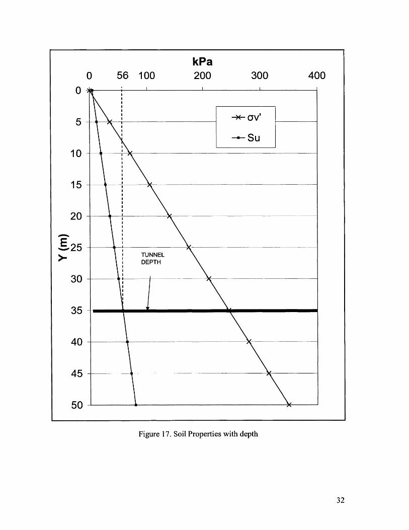
the undrained shear strength. For bored tunnels in Singapore the springline is typically

located at Z = 20-35m such that a,= 350-600kPa, Su= 30-5OkPa, hence the stability of

the face and the volume loss depends on the face pressure, at. For a deep clay situation

typical values of VL are 1-2%. The analyses in this thesis assume a constant value, VL

2%.

10

3.0 EMPIRICAL METHODS

These methods, derived from observed field measurements, are well-established and are

primarily used for estimating surface settlement, though there are some results available

for calculating subsurface movements. The following section will outline the empirical

methods available for a single tunnel, twin tunnels, for both surface and subsurface

ground movements.

3.1 SINGLE TUNNEL

Before the effects caused by twin tunnels are investigated it is important to understand

the effects of a single tunnel. Once this is done, the effects of two tunnels can be

calculated using the principle of superposition for surface settlement by analyzing

bending moments caused by the subsurface movements of one tunnel on another.

3.1.1 SURFACE EFFECTS

The most commonly used empirical method is that put forward by Shmidt (1966) who,

proposed that the settlement trough could be represented by a Gaussian distribution curve

(Figure 1).

S = S .ax. exp j (3)2i 2

Where: S= surface settlement at distance x from tunnel centerlineSmax = maximum settlement at x=Ox = distance from tunnel centre linei = the location of point of inflexion

11

Here, Smax can be calculated using the following equation:

Where:

0.313VLD 2 (4)

D is the diameter of the tunnel, and i is the lateral distance to the point ofinflection in the settlement trough.

Table 1: Inflection dimension proposed by various researchersAdditional

Name i-value Comments

Peck(1969) -= n 0.8 to 1.0R 2R)

i = 0.25(Z + R) :loose sand

Atkinson & Potts (1979) i = 0.25(1.5ZO +0.5R):dense _sand and over consolidated

clay

i = 0.43ZO +1.1 :Cohesive SoilO'Reilly & New (1982) -.~ 0 -. :rnlrSi

i = 0.28ZO - 0. 1:Granular Soil

Mair (1983) i = 0.5ZO

i (Z0 )Attewell et al (1977) -= a. a = I andn =1

R 2R

Clough & Schmidt i (Z 0 "-= a. n a= l and n =0.8(1981) R 2R

Where: Zo = Depth of the tunnel springline below ground surfaceR = Tunnel Radius

Using this table, equations 3 and 4 and assuming constant values for R, Zo and VL the

different i-values can be directly compared. For this the following values are assumed,

and resulting surface settlement trough plotted in Figure 1.

12

X (M)

0 5 10 15 20 25 30 350

VL= 2.0%R =3.5m .7-

5 - Zo =35m

10 -

3.12SBURAEEFET

o i-)-- Atkinson & Potts (1979)

-- O'Reilly & New (1982)

20 .,, -e -Peck (1969), M air (1983) andX.X Attewel et al (1977)

- X X- -X- -Clough & Schmidt (198 1)25 - --

30-

Figure 1. Surface settlement troughs from various empirical methods.

The values Of Smax, range from 17mm to 24mm and the location of the point of inflexion

ranges from 13.5m to 17.5m.

3.1.2 SUBSURFACE EFFECTS

Compared to surface settlement methods, there are few empirical methods to predict the

subsurface settlements and even fewer to predict lateral deformations. It is often assumed

that the subsurface settlement profiles developed during tunnel construction are also

characterized by a Gaussian distribution (Mair, 1993). Three of the most widely-used

methods are: Mair (1993), Atkinson & Potts (1979) and Vermeer et al. (199 1).

13

Mair (1993) proposed the following method:

S =S exp _X2

iz =k(Z 0 - Z)

0.175+0.325 1- Z

k= Z )

z

Szm =

(5)

(6)

(7)

0

1.2 5VL

0.175 + 0.325(

Sz,max = maximum settlement at depth, z, S, = Settlement at depth, z at

distance x from centerline

These equations can be used to find the settlement trough at any depth and can also be

used to find the settlement profile at any distance from the tunnel centerline.

Atkinson & Potts (1979) proposed the following method:

Sz = S 1.0 - a(Z--R)2R)

a = 0.57 for dense sanda = 0.40 for loose sanda = 0.13 for over consolidated clay

14

(8)

(9)

Where:

and,

Where:

R 2

Zo)

exp )(2i,

The final empirical method for estimating subsurface settlement was proposed by

Vermeer et al (1991):

0.8 /IZ - x2S , = O 0 Sz,aex p( .2

Z0 - R 2iz

In order to compare these three methods, two comparisons are required, one for a

constant Z and one for a constant x which can be seen in Figures 2 and 3 respectively.

Distance from Centreline (m)

0 5 10 15 20 25 30 350

5-

10

EE

15E

20-U- Mair (1993)

-X- Atkinson & Potts VL = 2.0%25 (1979) R = 3.5m

-A- Vermeer (1991) Zo 35m

30

Figure 2. Subsurface settlement troughs from various empirical methods (Z/Zo=0.5).

As with the surface troughs it can be seen that there is some variability in these methods

as the settlement values vary by about 9mm. However, all the methods are based on a

single iz value so the farther from the centre line the estimates are taken the closer the

results from each method become.

15

(10)

Settlement (mm)

0 5 10 15 20 250

5-1---U- Mair (1993)

10 - -X- Atkinson & Potts (1979)

- -- Vermeer (1991)

15

VL =2.0%f 20-- R =3.5m

- Zo 35m

25 x=Om

x=10m

30

35

40

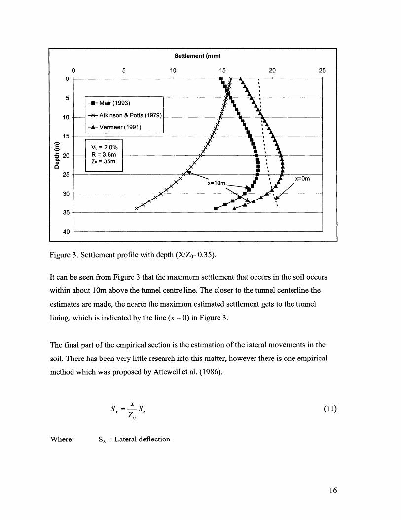
Figure 3. Settlement profile with depth (X/Zo=0.35).

It can be seen from Figure 3 that the maximum settlement that occurs in the soil occurs

within about 1 Om above the tunnel centre line. The closer to the tunnel centerline the

estimates are made, the nearer the maximum estimated settlement gets to the tunnel

lining, which is indicated by the line (x = 0) in Figure 3.

The final part of the empirical section is the estimation of the lateral movements in the

soil. There has been very little research into this matter, however there is one empirical

method which was proposed by Attewell et al. (1986).

SX = XS (1Zo

Where: S, = Lateral deflection

16

The lateral deflection is a function of the vertical settlement at a depth Z, and a distance x

from the centerline. Using the values for Sz from the previous methods Figure 4 is

plotted.

Lateral Deflection (mm)

0 -1 -2 -3 -4 -5 -6 -70

-a- Mair (1993), Norgorve (1979)

5-*- Atkinson & Potts (1979),

Norgrove (1979)10 -A- Vermeer (1991), Norgrove

(1979)

__15

E VL = 2.0%R = 3.5m

C20 ---- ZO = 35m

25

30

Z0=35m,

35

40

Figure 4. Lateral deflections from tunnel construction (X/ZO = 0.35).

This estimation doesn't take into account the volume loss that would be caused by lateral

deformation, as it takes a value of VL based only on the volume lost due to vertical

settlement. However, it does give a good indication of the profile of lateral deflection that

can be expected when constructing a tunnel in clay.

17

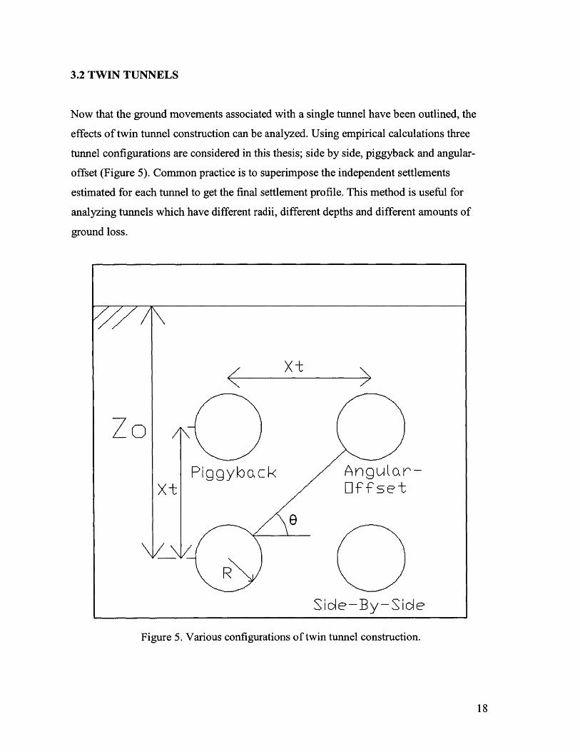
3.2 TWIN TUNNELS

Now that the ground movements associated with a single tunnel have been outlined, the

effects of twin tunnel construction can be analyzed. Using empirical calculations three

tunnel configurations are considered in this thesis; side by side, piggyback and angular-

offset (Figure 5). Common practice is to superimpose the independent settlements

estimated for each tunnel to get the final settlement profile. This method is useful for

analyzing tunnels which have different radii, different depths and different amounts of

ground loss.

/

xt

7A

Piggyback Angutar-Offset

R 0

Side-By-Side

Figure 5. Various configurations of twin tunnel construction.

18

Zo

/7 \

While this is very useful for quick analysis of the effects of twin tunnels it does not take

into account many aspects of tunnel construction which could have a significant effect on

the magnitude of settlement, such as:

" Length of time between driving tunnels

* Consolidation movement

" Assumes first tunnel has no effect on ground displacements caused by second

tunnel

For the comparison of the effects of twin tunnel construction the distance and position of

the tunnels will be varied, while the same values used for the comparison of the single

tunnel ground movement will be used. This will be done for a side-by-side tunnel, a

piggyback tunnel and a tunnel at a relative angular position of 450, each at a distance of

15m.

19

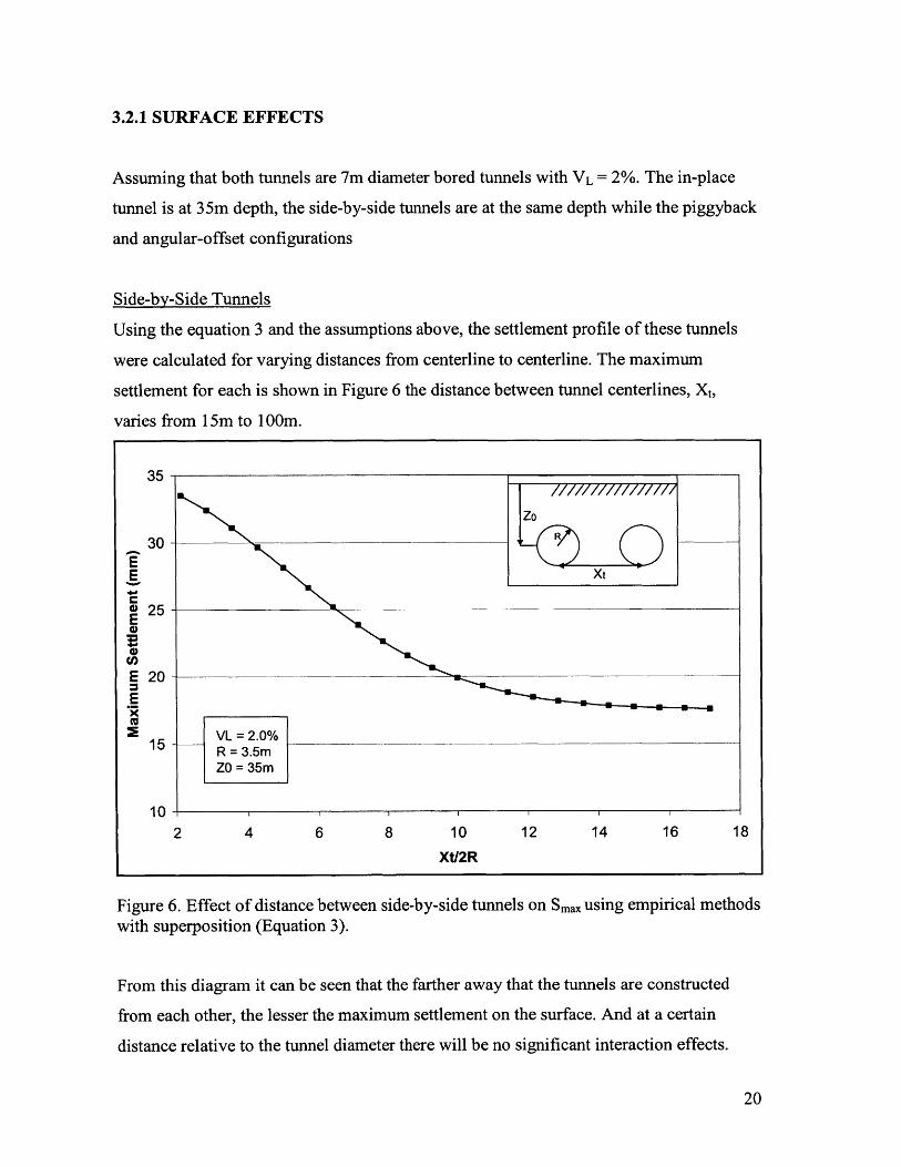
3.2.1 SURFACE EFFECTS

Assuming that both tunnels are 7m diameter bored tunnels with VL = 2%. The in-place

tunnel is at 35m depth, the side-by-side tunnels are at the same depth while the piggyback

and angular-offset configurations

Side-by-Side Tunnels

Using the equation 3 and the assumptions above, the settlement profile of these tunnels

were calculated for varying distances from centerline to centerline. The maximum

settlement for each is shown in Figure 6 the distance between tunnel centerlines, Xt,

varies from 15m to l00m.

35-

Zo

30 -____1111111111111777

E Xt

S25-E

U)

E 20E

15 -- VL =2.0%R = 3.5mZO = 35m

10

2 4 6 8 10 12 14 16 18XtI2R

Figure 6. Effect of distance betweenwith superposition (Equation 3).

side-by-side tunnels on Smax using empirical methods

From this diagram it can be seen that the farther away that the tunnels are constructed

from each other, the lesser the maximum settlement on the surface. And at a certain

distance relative to the tunnel diameter there will be no significant interaction effects.

20

Settlement increases as the tunnels get closer due to the combined effect of the volume

loss parameters. In general practice, tunnels will not be built within 2 diameters of each

other's center line. In figure 7, the settlement profile can be seen for Xt ~ 4R. The effect

of the second tunnel clearly creates a much deeper trough (32mm as opposed to 18mm).

X(m)

-35 -25 -15 -5 5 15 25 35

-20-E

E

U)

40 N//Zo 15m

--- First Tunnel Only VL = 2.0% 50 R-i- Second Tunnel Only R = 3.5m R

- Superimposed ZO = 35m

60

Figure 7. Empirical settlement trough for side-by-side tunnels at Xt/R = 4 bysuperposition of empirical equations (Equation 3).

The increased gradient on the surface can cause difficulties if building in a sensitive area,

such as beneath an urban area so therefore this analysis of the settlement could be used to

find the optimum distance between the tunnels in order to optimize cost vs. risk.

21

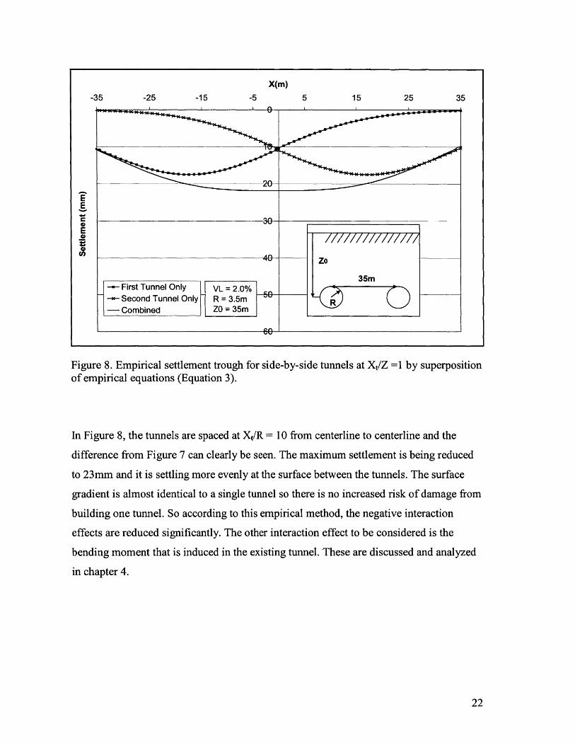
X(m)-35 -25 -15 -5 5 15 25 35

0

E

30E

35m--First Tunnel Only VL =2.0% -5

--- Second Tunnel Only R = 3.5m R-Combined ZO = 35m

60

Figure 8. Empirical settlement trough for side-by-side tunnels at Xt/Z =1 by superpositionof empirical equations (Equation 3).

In Figure 8, the tunnels are spaced at Xt/R = 10 from centerline to centerline and the

difference from Figure 7 can clearly be seen. The maximum settlement is being reduced

to 23mm and it is settling more evenly at the surface between the tunnels. The surface

gradient is almost identical to a single tunnel so there is no increased risk of damage from

building one tunnel. So according to this empirical method, the negative interaction

effects are reduced significantly. The other interaction effect to be considered is the

bending moment that is induced in the existing tunnel. These are discussed and analyzed

in chapter 4.

22

Piggyback Tunnels

The interaction of the piggyback configuration introduces a new issue relating to the

order of construction. For side-by-side tunnels it is assumed that there is no difference if

one is built before the other. However, with piggyback tunnels there can be an increased

interaction as a result of constructing one tunnel above or below the other. This is not

considered in the empirical analyses which are based on superposition, but can

considered using numerical analyses, chapter 4. In Figure 9, the effect that the distance

between the two tunnels has on the maximum settlement can be seen.

80 -

75

70

65 -

60 t-

55

50

45

402 2.2 3.82.4 2.6 2.8 3 3.2 3.4 3.6

Xt/2R

Figure 9. Effect of distance between piggy back tunnelsof empirical solutions (Equation 3)

on Smax based on superposition

In the analysis for Figure 9, the first tunnel was taken to be the same as previous

examples and the upper tunnel's location varied from 20m to Im. As can be seen from

Figure 9, the closer the tunnel is constructed to the surface the larger the maximum

settlement is estimated to be. This is due to the subsurface settlements increasing as

measurements are taken nearer to the tunnel. An empirical piggyback trough can be seen

in Figure 10 for tunnels at 3 5m and 20m depth.

23

Zo

Xt

R

E,E

E

0)

EE.R

VL = 2.0%R = 3.5mZO = 35m

85

X(m)

-35 -25 -15 -5 5 15 25 35

-+0-

E40 Zo

a)

50

15m

-U- Lower Tunnel Only VL = 2.0% _0

-)- Upper Tunnel Only R = 3.5m


70

Figure 10. Settlement trough for piggyback tunnels by superposition of empiricalequations (Equation 3).

Since the upper tunnel is the one that causes more settlement and therefore the most

damage, it is more logical to place the upper tunnel as low as possible. This will create a

problem of changing the bending moment in the existing tunnel. Therefore a solution will

be looked at in the finite element section (chapter 4) for optimizing the design based on

the induced bending moment and the distance between the tunnels.

It is not easy to reduce the settlement in piggyback tunnels because depth is a limiting

factor. In side by side tunnels this poses less of a problem as you can move the tunnels

farther and farther away from each other without having to go deeper, hence the

interaction effects can be significantly reduced with relatively low increase in cost.

24

Angular-offset Tunnels

If there was inadequate space for a side-by-side or piggyback tunnel, a third option would

be to locate the second tunnel at an angular-offset position. The current example assumes

the two tunnels are aligned at 450 to each other, and varies the spacing, Xt. As with

piggyback tunnels, the issue arises of which tunnel should be constructed first, which will

not be addressed in empirical superposition. Figure 11 shows the effects of distance

between the tunnels on Smax, assessed with the first tunnel located at Zo = 35 and the

second at depths ranging from 24m to 1 Om.

70 -

65 -Zo

xt60 -- 45*

60-E

d 55

E

50 -U)

40

40 VL =2.0%R = 3.5m

35 - ZO = 35m

302 2.5 3 3.5 4 4.5 5 5.5

Xt/D

Figure 11. Effect of distance between angular tunnels onempirical equations (Equation 3)

Smax using superposition of

This creates a similar graph to the piggyback tunnels but with some key differences. The

combined settlement is much lower in this method (e.g. for Xt/2R ~2, Smax = 75mm and

45mm for piggyback and angular-offset configurations, respectively). It is possible to

construct the tunnel much farther away (Xt/2R < 5) here at an angular-offset of 45*.

25

-40 -30

E

E

U)

-20 -10X(m)

0

Figure 12. Empirical settlement trough for angular-offset tunnel using superposition ofempirical equations (Equation 3).

Figure 12 shows the empirical settlement trough for angular-offset tunnels at 450 with the

first tunnel at 35m depth and the second at 24m depth. The settlement above the lower

tunnel is much less than the settlement above the upper tunnel, therefore when the

superimposed curve is created the maximum settlement is almost directly above the upper

tunnel. During design angular tunnels the upper tunnel should be positioned where the

resulting settlement would cause the least damage.

26

10

30

Zo15.5m

45-*- Lower Tunnel Only VL = 2.0% ,,--- Upper Tunnel Only R = 3.5m


10 20 30 40


The vertical settlement troughs for the subsurface are very similar to the settlement

troughs for the surface, therefore there is no need to plot the data again as we can assume

that the same patterns will be seen in the subsurface. However, it is still important to

consider the lateral movement throughout the soil for the same three situations used in

section 3.2.1: 1) a side-by-side tunnel 2) a piggyback tunnel and 3) a 450 angular-offset

tunnels. For this section equation 11 (Attewell et al, 1986) is used to superimpose lateral

movements in soil.

Side-By-Side Tunnels

In this situation, due to the principal of superposition it is assumed that for values of x

directly in the centre of the two tunnels the lateral movements will be zero. Therefore the

values will be found only for directly above each tunnel. Figure 13 shows the lateral

movement with depth, estimated above each tunnel.

Lateral Movement (mm)

-10 -8 -6 -4 -2 0 2 4 6 8 10

---

10

-01

25 Sx>O

-eAbove First Tunnel /--x- Above Second Tunnel iZ Zo

VL = 2.0% 35 -R = 35m15m

40

Figure 13. Lateral Movements with depth for side-by-side tunnelsempirical equations (Equation 11).

using superposition of

27

From Figure 13 it can be seen that the estimated deflections above each tunnel are equal

in magnitude and opposite in direction. At the center of the first tunnel there is no

movement caused the construction of the first tunnel, so the movements which will occur

are caused solely by the construction of the second tunnel, and similarly the movements

above the second are caused solely by the construction of the first tunnel. Figure 14

shows the lateral movement between the tunnels at 35m depth.

8VL = 2.0%R = 3.5m

-ZO= 35m 6

E

02

-- First Tunnel Only---Second Tunnel Only -

- Superimposed

-8

X (M)

Figure 14. Lateral movements estimated between side-by-side tunnels usingsuperimposition of empirical equations (Equation 11).

Using this method the maximum lateral movements are estimated to occur at one quarter

of the distance between the tunnels, in each direction. The final movements that occur as

a combination of both tunnels are smaller than the movements which occur for each

tunnel separately. Although this appears satisfactory, the soil is in fact moving for one

tunnel and then back as the second tunnel is constructed.

28

Piggyback Tunnels

Since lateral movement above the centerline of each tunnel is zero there will be only

vertical deformations between these tunnels. The effect seen in the side-by-side tunnels

where the lateral movements 'cancel out' will not be seen here, which means that the net

lateral movements will be accumulative. In Figure 15 the lateral deformation is plotted

with depth at x = I Om.

-.E)

Horizontal Movements (mm)

.10-20 -15

V1V

-U- Lower Tunnel Only--- Upper Tunnel Only

-Superimposed

K

VL = 2.0%R = 3.5mZO = 35m k

-5 0 5

V15

Figure 15. Lateral deformations for piggyback tunnels atof empirical solutions (Equation 11)

X=IOm using superimposition

The maximum lateral movement for piggyback tunnels is -0mm which occurs quite

close to the surface in this example. The lateral movement increases with distance until it

peaks then begins to decrease.

29

X=10m

Zo

15m

R

10 20

- -

-1

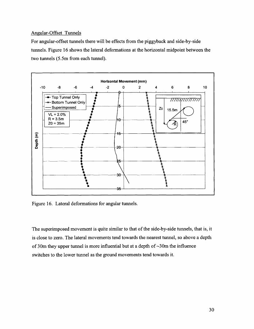
Angular-Offset Tunnels

For angular-offset tunnels there will be effects from the piggyback and side-by-side

tunnels. Figure 16 shows the lateral deformations at the horizontal midpoint between the

two tunnels (5.5m from each tunnel).

-8 -6 -4

Horizontal Movement (mm)

-2 0 2

--- Top Tunnel Only-u- Bottom Tunnel Only

- Superimposed Zo 15.5mVL = 2.0%R = 3.5m 0

20

54

35

Figure 16. Lateral deformations for angular tunnels.

The superimposed movement is quite similar to that of the side-by-side tunnels, that is, it

is close to zero. The lateral movements tend towards the nearest tunnel, so above a depth

of 30m they upper tunnel is more influential but at a depth of-30m the influence

switches to the lower tunnel as the ground movements tend towards it.

30

-10

E.

CL4)

4 6 8 10

4.0 FINITE ELEMENT ANALYSIS OF TWIN TUNNELS IN SINGAPORE

MARINE CLAY

Plaxis is a finite element program used for soil and rock analyses, it is used in this section

to analyze the same situations as outlined in the empirical methods. This section breaks

down into the analysis of ground movement and the analysis of the stresses in the tunnel

lining.

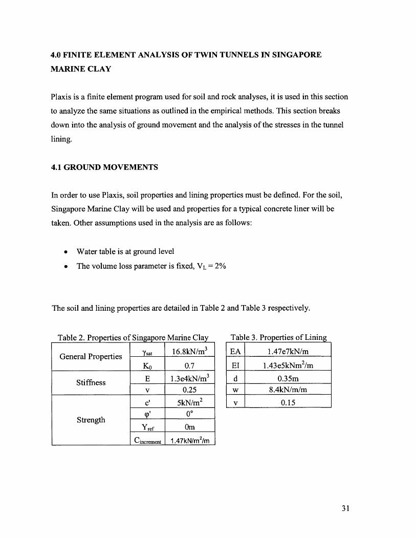
4.1 GROUND MOVEMENTS

In order to use Plaxis, soil properties and lining properties must be defined. For the soil,

Singapore Marine Clay will be used and properties for a typical concrete liner will be

taken. Other assumptions used in the analysis are as follows:

" Water table is at ground level

" The volume loss parameter is fixed, VL =2%

The soil and lining properties are detailed in Table 2 and Table 3 respectively.

Table 2. Properties of Singapore Marine Clay

General Properties Ysat 16.8kN/m'Ko 0.7

Stiffness E 1.3e4kN/m 3

v 0.25

c' 5kN/m 2

Strength 00Yref Om

Cincrement 1.47kN/m2/m

Table 3. Properties of Lining

EA 1.47e7kN/m

El 1.43e5kNm 2/m

d 0.35mw 8.4kN/m/m

v 0.15

31

kPa0 56 100 200 300

0

5

10

15

20

E,25

30

35

40

45

50

400

Figure 17. Soil Properties with depth

32

TUNNELI DEPTH

4.1.1. SURFACE EFFECTS

In order to check that superposition is applicable in tunnel design the settlement troughs

for each tunnel are found separately and then superimposed. An analysis will then be run

for both tunnels and the resulting trough will be compared to the superimposed trough.


Figure 18 shows the effect of distance on the maximum settlement. The nearer the

tunnels are the larger the settlement is, but at a certain distance the maximum settlement

will not decrease further, which corresponds to Smax for a single tunnel.

24

Singapore Marine ClayVL = 2.0%

22 R = 3.5m ZoZO =35m Xt

R20

E 18

E 16

14 - _ _ _ _ _ _ _ _ _ _ _ _

12-

10-3 4 5 6 7 8 9 10

Xt/2R

Figure 18. Effect of distance between tunnels on Smax.

33

E,E

E

X(m)

-100 -80 -60 -40 -20 0 20 40 60 80 100

Figure 19. FE Settlement troughs for side by side tunnels (Xt=15m)

X (m)

-100 -80 -60 -40 -20 0 20 40 60 80 100

X

25

ie 20.gaprseMmrenE frth TunnelsZ

25

Figure 20. FE settlement troughs for side-by-side tunnels (Xt = 35m)

34

\ 4 ''' '

Singapore Marine Clay

VL = 2.0%R = 3.5mZO = 35m

__--First Tunnel Only A Zo 15m --A- Second Tunnel Only-Superimposedx-FIE for Both Tunnels

Figure 19 and 20 show side-by-side tunnels for tunnels spaced at 15m and 35m,

respectively. For the closely spaced tunnels (Xt = 15m) the superimposed curve almost

exactly matches the numerical results. Superimposition over-estimates Smax by 2mm.

Even if there is a small difference superposition obviously works well for closely spaced

tunnels. Figure 20 shows a similar chart for widely spaced tunnels (Xt = 35m), the

superimposed and FE curves align a lot closer in this chart, although there is a fraction of

a millimeter difference at the trough, so superposition works very well for closely and

widely-spaced side-by-side tunnels.

Piggyback Tunnels

X (m)

-100 -80 -60 -40 -20 0 20 40 60 80 100

%'

E4)

1V Zo-co

-e Top Tunnel Only Singaporeoe- Bottom Tunnel Only Marine Clay 15m-- eSuperimposed d trou--- Top Tunnel First VL =32.5%--e- Bottom Tunnel First ZO = 35m

25

Figure 2 1. FE Settlement troughs for piggy back tunnels (Xt =I5m)

For the finite element analysis of piggyback tunnels two situations have to be considered,

one for the top tunnel constructed before the bottom tunnel and one for the bottom tunnel

constructed before the top. In Figure 21 both of these situations have been plotted with

the superimposed trough.

35

The trough for constructing the upper tunnel first and the trough for constructing the

lower tunnel first are very close together and gave a result for the maximum settlement of

19mm. Therefore, the order of construction has very little effect on the final settlement

trough, in this example. The results show less then 2mm difference in the maximum

settlements compared to direct superposition settlement and practically identical results

for X > 25m.

In a separate set of analyses the maximum settlement was checked for varying values of

Xt, the distance between the piggyback tunnels. The results show very little variation in

the maximum settlement as the upper tunnel was progressively moved from a depth of

20m to a depth of 1Gm. The settlement occurring was -9mm with a variance of ~1mm.

This shows that, in finite element analysis, the vertical effects of piggyback tunnels do

not interfere significantly with the maximum settlement.

36


44

42

E40E

E 38

E 36E

S34

32

302 2.5 3 3.5 4 4.5

I XtI2R

Figure 22. Effect of distance between angular tunnels on Smax

Figure 22 shows the maximum settlement computed for varying distances between two

450 angular-offset tunnels. The results show a linear decay with spacing between the two

tunnel bores.

However, looking at the trends for side-by-side and piggyback curves, the maximum

settlement would be expected to reach its minimum value at Xt/2R ~ 10, so for a 450

angle in order to achieve this the lower tunnel would have to be at a depth, ZO > 50m.

37

Singapore Marine Clay

VL = 2.0%R = 3.5mZO = 35m Zo X

450

R

-80 -60 -40 -20 20 40 60 80X(m)

0-1

E

E40

0E)

Figure 23. FE settlement troughs for Angular Tunnels (Xt=1 5m)

Similarly to the piggyback tunnels there is an issue with the order of construction of

angular-offset tunnels. Fig 23 shows the troughs for each situation.

The surface settlement troughs for constructing tunnels in different sequences are very

similar and produce settlement differences less than 2mm. This shows that the order of

construction has no effect on the final settlement trough for the soft clay conditions

considered in this case.

The superposition curve is almost identical to the trough for constructing the lower tunnel

first and very close to the trough for constructing the upper tunnel first. Therefore, it can

be seen that superposition works extremely well when estimating settlement for the 450

angular-offset tunnels.

38

50in

- Top Tunnel Only Singapore Zo-*- Bottom Tunnel Only Marine Clay 15.5m0

- Superimposed VL = 2.0%-*-Top Tunnel First R = 3.5m-+- Bottom Tunnel First ZO = 35m

00 100


Considering that the vertical settlement profiles with depth are very similar to the

settlement profiles for the surface it can be assumed that similar patterns will be seen.

This section compares the lateral movements estimated by Plaxis, and determines

whether or not the principle of superposition can be applied based in non-linear finite

element analysis.



-'5 -10 -5 / 5 10 15

-5-u-Above Second Due To First--- Above First due to Second Z-- Above First Tunnel 15m

-- Above Second Tunnel

4 C R

Singapore Marine Clay*0

VL = 2.0%R = 3.5m 2

ZO = 35m 2

-- 30-

35

Figure 24. FE Lateral movements with depth for side-by-side tunnels

In Figure 24, it can be seen that the lateral movements above the first tunnel are almost

symmetrical to the lateral movements above the second tunnel, with the largest variance

being ~-Imm. Considering that there are zero lateral movements above each tunnel due to

the construction of that tunnel and that the effects of the opposite tunnel are very close to

the final settlement, this shows that superposition works.

39

50

-i- First Tunnel Only 4_0-i- Second Tunnel Only

- Superimposed 30-0>- FE for Both

20E

E

0

-50

X(m)

Figure 25. FE Lateral movements estimated between side-by-side tunnels

In Figure 25 the lateral movements were calculated for the space between the tunnels. It

can be seen that when combined, the lateral movement calculated exactly in between the

tunnels is zero. The superimposed curve roughly aligns with the finite element curve for

the second tunnel, however, near the first tunnel there is a significant discrepancy (Sx =

7mm). In this zone between the two tunnels, the plastic zones for each tunnel will

intersect, which will almost always cause severe plastic deformation. Therefore,

superposition will suggest approximate results but is not very accurate, in this example.

40

Piggyback Tunnels


0 5 10 15 20 25 300-

Singapore Marine Clay -u- Top Only

VL = 2.0% -- Bottom Only

10 R = 3.5m -SuperimposedZO = 35m -*- FE for Both Tunnels

20_ _

lom

= 30Zo

40

15m

50 R

60

Figure 26. FE Lateral deformations for piggyback tunnels (x = 1Om)

For piggyback tunnels, the lateral deformations were estimated for a vertical profile at a

horizontal distance of 1 Om. These movements will be symmetrical on the other side of

the tunnel centerline. For the upper tunnel only, the minimum movement occurs at the

level of the tunnel (at depth of 20m) whereas for the lower tunnel only the minimum

movement occurs much nearer the surface. Regardless of this, the superimposed curve

matches the combined curve within -4mm until a depth of about 30m where the

combined FE analysis begins to gradually increase with respect to the corresponding

superimposed value.

41


-0 -20 -10 10 20 30

Zo15.5m

R

40

Singapore --- Top OnlyMarine Clay,-Botmny

VL = 2.0% -- SuperimposedR = 3.5m -- FE for Both TunnelsZO = 35m

-60Lateral Movements (mm)

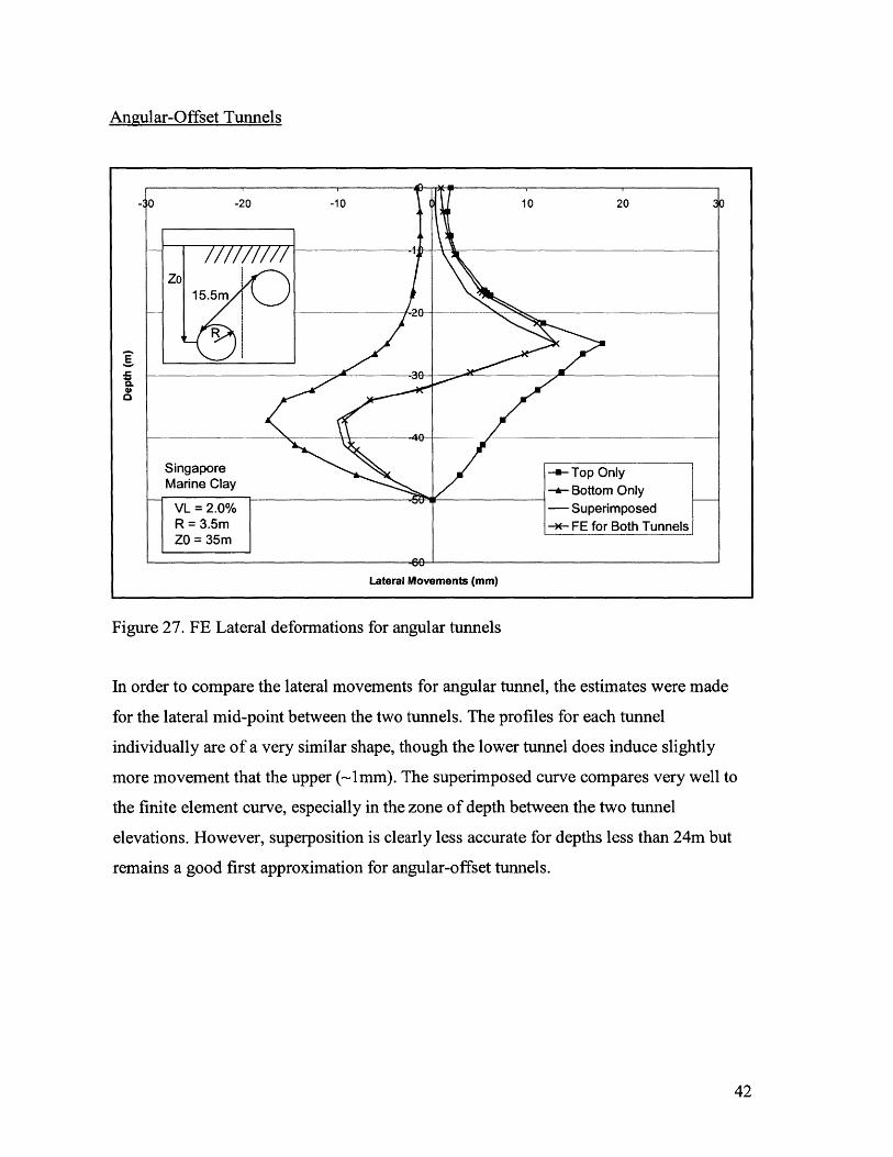
Figure 27. FE Lateral deformations for angular tunnels

In order to compare the lateral movements for angular tunnel, the estimates were made

for the lateral mid-point between the two tunnels. The profiles for each tunnel

individually are of a very similar shape, though the lower tunnel does induce slightly

more movement that the upper (-mm). The superimposed curve compares very well to

the finite element curve, especially in the zone of depth between the two tunnel

elevations. However, superposition is clearly less accurate for depths less than 24m but

remains a good first approximation for angular-offset tunnels.

42

Plastic Deformations

The comparison between the superimposed solutions and the finite element solutions

illustrate that superposition applies very well to these situations. The discrepancies that

occur in the solution are caused by the plastic deformation that occurs in the soil

immediately surrounding the tunnels. In Figure 28, the plastic zone for twin tunnels

located at 15m from centerline to centerline is shown.

mu

U U

*. ;iU I

0 PLASTIC POINT IN FINITE ELEMENT MESH

Figure 28. Plastic Zone surrounding side-by-side tunnels (Xt/2R = 2.2).

The zone of plasticity surrounding each tunnel is roughly equal to the radius of the tunnel

(3.5m). Using this zone of plasticity and comparing it to Figure 18, it is seen that the

location of the largest difference between the curves corresponds to the centre of the

combined plastic zone from the two tunnels. Similarly for the piggyback and angular

situations the plastic zones correspond to the areas where superposition breaks down.

43

UU

U

a * * ** U U U

U. *I~

U

a U

* U

* U

U U

p

M

VL = 2.0%R =.5mZO = 35m

4.2 LINING STRESSES

Estimates of surface settlements due to tunneling are very important in order to mitigate

potential damage to adjacent structures. However, it is also very important to predict the

expected forces and deformations that will be seen in the adjacent tunnel lining so that

the correct design can be made for the tunnel. For example, in an underground subway

tunnel, if the tunnel deforms more than expected or if the bending moment induces a

crack in the lining then the functionality of the tunnel is compromised. This section

consists of structural lining interaction between twin tunnels. The same examples that

were used in the previous sections are used again.

The force used to measure and compare each situation is the bending moment in the

liner, which is plotted against varying values of Xt/2R. For each analysis there are three

bending moments which are:

" Bending moment in the first tunnel due to the construction of the first tunnel

" Bending moment in the first tunnel after the construction of the second tunnel

" Bending moment in the second tunnel due to the construction of the second tunnel

44

4.2.1 SIDE-BY-SIDE TUNNELS

120

-- First Tunnel Before Second-x-First Tunnel After Second

100+ Second

E

S800

E0

0

E 40 ZE 1S

15m

20 . VL =2.0%R = 3.5m CZO = 35m

2 3 4 5 6 7 8 9 10

Xt/2R

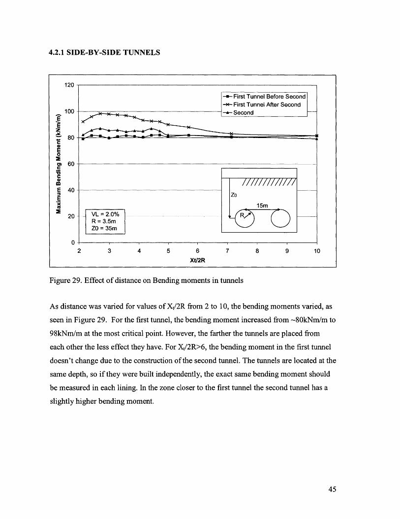
Figure 29. Effect of distance on Bending moments in tunnels

As distance was varied for values of Xt/2R from 2 to 10, the bending moments varied, as

seen in Figure 29. For the first tunnel, the bending moment increased from -80kNm/m to

98kNm/m at the most critical point. However, the farther the tunnels are placed from

each other the less effect they have. For Xt/2R>6, the bending moment in the first tunnel

doesn't change due to the construction of the second tunnel. The tunnels are located at the

same depth, so if they were built independently, the exact same bending moment should

be measured in each lining. In the zone closer to the first tunnel the second tunnel has a

slightly higher bending moment.

45

Moments in Tunnel Lining

The following three figures show the bending moments at each stage of the construction

process of a 15m spaced side-by-side tunnel. Figure 30 shows the bending moment in the

first tunnel by itself. The maximum moment is seen in the tunnel springline. The moment

distribution is symmetrical for this case.

Figure 30. Bending Moment in First Tunnel Only - Max BM = 79.48kNm/m

After the construction of the second tunnel the bending moment diagram changes shape

slightly (Figure 31). The maximum moment is now seen in the left springline, on the far

side from the new tunnel.

Figure 31. Bending Moment in First Tunnel After second tunnel - Max BM =93.15kNm/m

46

Finally, the moment seen in the second tunnel after its construction is shown in Figure

32. The maximum bending moment for the second tunnel is seen in the right springline,located on the far side from the first tunnel.

Figure 32. Bending moment in Second Tunnel - Max BM = 82.59kNm/m

47

4.2.2 PIGGYBACK TUNNELS

100-

90

80.

E 70I -m- Bottom tunnel before topzdi 60- x Bottom tunnel after top

-- Top TunnelE 50-0

0)40-

30 -

20-

10

02 2.2 2.4 2.6 2.8 3 3.2 3.4

Xt/2R

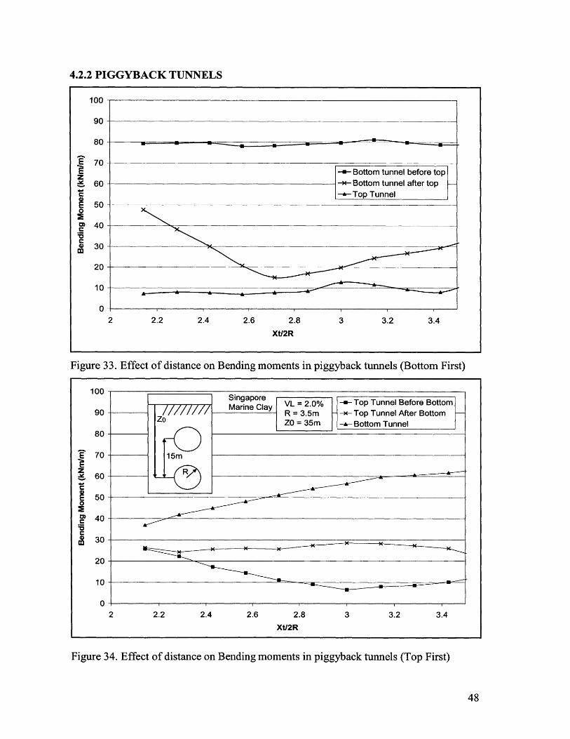
Figure 33. Effect of distance on Bending moments in piggyback tunnels (Bottom First)

z

0)

100

90

80

70

60

50

40

30

20

10

02.4 2.6 2.8 3 3.2 3.4

Xt/2R

Figure 34. Effect of distance on Bending moments in piggyback tunnels (Top First)

48

2 2.2

Mineaplay VL =2.0% -- Top Tunnel Before Bottom

- Mrie Za R =3.5m -x- Top Tunnel After Bottom -Zo ZO =35m -- Bottom Tunnel

15m

The analysis for the piggyback tunnels is shown in Figures 33 and 34. Figure 29 shows

the situation where the bottom tunnel (at Zo = 35m) was constructed before the upper

tunnel. The location of the upper tunnels varies for Xt/2R = 2 to 3.4 such that the

shallowest upper tunnel is at Z = 1Gm. The limit of 3.4 arises from the minimum depth of

the upper tunnel of -1 Gm. Figure 30 shows the situation where the upper tunnel was

constructed before the lower tunnel, but the location of the upper tunnel was varied

exactly as for the situation when constructing the bottom tunnel first.

In Figure 33, the bending moment for the lower tunnel is constant (Zo = 35m), but when

the upper tunnel is constructed there is a large reduction in the lower bending moment

from -80kNm/m to 15kNm/m, in the most severe situation (an 80% decrease). This

trough occurs at Xt/2R = 2.7 and at higher values the bending moment is starting to

increase. However, since the tunnels cannot be placed at much further distances, the

effects cannot be determined.

In Figure 34, the independent bending moment for the upper tunnel increases with depth,

and increases significantly after the construction of the lower tunnel. This result occurs

due to settlement produced by the construction of the lower tunnel. When the lower

tunnel is constructed the upper tunnel will settle further than the ground above it, which

will increase the vertical stress and therefore the bending moment in the tunnel lining.

Even though the final stresses are different for both situations, the sum of the maximum

bending moments is more consistent. For any value of Xt in Figure 33, if the final

moment in the lower tunnel is less than in Figure 34, the moment for the upper tunnel is

greater. Therefore, in order to reduce a higher moment in either of the two tunnels, the

upper one should always be constructed first.

49

4.2.3 ANGULAR-OFFSET TUNNELS

140--- Bottomn Tunnel Before Top-- Bottomn Tunnel After Top

120- Top Tunnel

100-

z

80-4)E0

0)60-

(D

M 40-

20-

0-2 2.5 3 3.5 4 4.5 5

XtI2R

Figure 35. Effect of distance on lining stresses in angular tunnels (bottom first)

140 Singapore Marine Clay

-i- Top Tunnel Before Bottom VL = 2.0%120 -- -Top Tunnel After Botom - R = 3.5m Zo 15.5

-+--Bottom Tunnel ZO =35m 45*

100

z80

600)

40-

20

02 2.5 3 3.5 4 4.5 5

Xt/D

Figure 36. Effect of distance on lining stresses in angular tunnels (top first)

50

The analysis for the 450 angular-offset tunnels is shown in Figures 35 and 36. Figure 35

shows the situation where the lower tunnel (35m depth) was constructed before the upper

tunnel, located at 45* from the horizontal plane. The location of the upper tunnel is varied

in the range Xt/2R = 2 to 5 (with minimum Z = lOim for the upper tunnel). Figure 35

shows the situation where the lower tunnel is constructed first.

In Figure 35, the bending moments calculated for the lower tunnel (Zo =35m)

M = 80kNm/m. Although unlike the piggyback tunnel, when the upper tunnel is built, the

moment in the lower tunnel increases. The largest increase is at Xt/2R = 2, where it

increases to 11 6kNm/m (45% increase). As the tunnels are placed at further and further

distances apart the increase is reduced to about 5kNm/m (6%).

In Figure 36, the bending moment calculated for the upper tunnel (Zo = 1 Om - 25m),

before the lower tunnel is constructed, varies depending on the depth at which the tunnel

is constructed. After the construction of the lower tunnel, the bending moment in the

upper tunnel increases by -1 8kNm/m until Xt/2R = 4.2, when it begins to level out and

have no effect. The moment in the lower tunnel ranges from 11 6kNm/m to a minimum

level of 80kNm/m.

Unlike the piggyback tunnels, the final moments calculated in the upper and lower

tunnels are very similar. This shows that the order of construction has no significant

effect on the bending moments in either tunnel.

51

5.0 COMPARISON OF NUMERICAL AND EMPIRICAL RESULTS FOR TWIN

TUNNELS

This section is directly compares the numerical solutions using non-linear finite element

analysis methods (Chapter 4) with empirical methods (Chapter 3).

5.1 COMPARISON OF NUMERICAL AND EMPIRICAL GROUND

MOVEMENTS

5.1.1 Side-By-Side Tunnels

X(m)-35 -25 -15 -5 5 15 25 35

1 G

E 02

40

Zo-+- Empirical (VL = 2%) R = 3.5m 1 5m1- FE (VL=2%) Zo = 35m f

--- Empirical (VL=1.4%)

60

Figure 37. FE vs. Empirical surface settlement trough for side-by-side tunnels

Figure 36 shows the surface settlement for side-by-side tunnels. Directly compared the

empirical trough gives a much larger settlement. However, using a VL Of 1.4% which

matched the Smax for the finite element analysis, a better comparison is seen. The FE

trough is always wider than the empirical trough which is consistent with results

published in the literature (e.g. Addenbrooke et al.,1997).

52

-10 -8 -6 -4


-2 0 2

a.a)

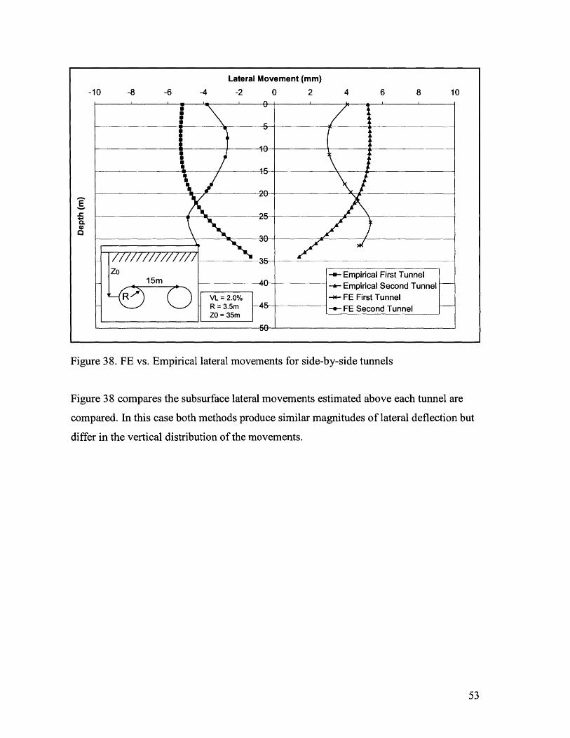
Figure 38. FE vs. Empirical lateral movements for side-by-side tunnels

Figure 38 compares the subsurface lateral movements estimated above each tunnel are

compared. In this case both methods produce similar magnitudes of lateral deflection but

differ in the vertical distribution of the movements.

53

' ''Zo':

5

20

x 25

ZO -5mA- Empirical First Tunneli 15 , 4 -w Empirical Second Tunnel

" RVL =2.0% -- FE First Tunnel-R = 3.5m 45--FE Second Tunnel --

ZO = 35m

A n

4 6 8 10

30

-- EmpiricalA FE

VL = 2.0% 20- -

R = 3.5mZO =35m

E 1 -

E

E

5 -4 -3 -2 -1 12 3 4 i

-10

Zo15m

20

30

X(m)

Figure 39. FE vs. Empirical lateral movements between side-by-side tunnels

Figure 39 shows the comparison of lateral movements in the zone directly between the

two tunnels. There is a huge difference, with empirical methods estimating 1-2mm of net

lateral movement, while finite element estimates 30mm. However, both methods estimate

a net movement of zero at the mid-point between the tunnels. The plastic zone, which is

located at a 3.5m zone surrounding the tunnel, is the cause for the large difference, as the

two plastic zones are so close to each other. For the lateral deformations the finite

element analysis computes a much larger lateral movement than the empirical methods.

54

5.1.2 Piggyback Tunnels

X (m)

Figure 40. FE vs. Empirical surface settlement troughs for piggyback tunnels

Lateral Movement (mm)0 -5 -10 -15 -20 -25

0

5 VL = 2.0% -R = 3.5m - 777~ZO =35m Zo

10

15 1515Sm

20

25

30-i- Empirical-'- FE

35

40

55

40

-30

\1 ZO

5015m

-- Empirical (VL =2%)---- FE (VL = 2%) 6-0 VL=20 R/

--- Empirical (VL =0.85%) R=3.5mZO = 35m

7n

E

Figure 41. FE vs. Empirical lateral movements for piggyback tunnels

-35 -25 -15 -5 5 15 25 35

Figures 40 and 41 show the comparison for surface and subsurface movements for

piggyback tunnels (lower tunnel constructed first), respectively. The surface settlement

profile shows a huge difference in maximum settlement, 19mm for the finite element and

48mm for the empirical. The indirect comparison, using a VL= 0/85% shows that even if

the maximum settlements are the same that the Finite element trough is wider.

The lateral movements, in Figure 41, are estimated at a distance of 1Gm from the tunnel

centerlines. The empirical methods estimate a larger deformation above the upper tunnel

with minimum deflection at the springline of the upper tunnel (Sx ~ 5mm). In contrast the

FE analyses show larger lateral deflections around the lower tunnel (Sx 20mm at the

springline).

5.1.3 Angular-Offset Tunnels

X(m)-35 -25 -15 -5 5 15 25 35

A

E1

30

ZoEmpirical (VL = 2%) 15.5m

-A- FE (VL = 2%)Empirical (VL = 1%) VV = 2.0%-

ZO = 35m

60

Figure 42. FE vs. Empirical surface settlement troughs for angular tunnels

56

Figure 42 shows the settlement troughs for 45 angular-offset tunnels spaced at 15.5m

(lower tunnel constructed first). As in the previous comparisons, the maximum settlement

for the empirical analysis is higher than the finite element estimate. In this situation, the

estimate is double, being 20mm and 40mm respectively. The finite element trough is

much wider than the empirical trough. Using VL = 1%, the finite element trough is again

shown to be wider.

Lateral Movements (mm)

-15 -10 -5 0 5 10 15W

ZO 15.5m 10

VL =2.0%R = 3.5m 2ZO = 35m

2350 -e-Empirical ~-F- F

35

Figure 43. FE vs. Empirical lateral deformations for angular tunnels

Figure 43 shows the estimated lateral movements for 45* angular-offset tunnels, taken at

the midpoint between the two tunnels. The net movements for the empirical methods are

very low (Omm-lmm). The finite element curve shows a maximum deformation of

13mm. The reason for this is related to the plastic zone that is in close proximity to the

midpoint of the tunnels. The elastic theory used in empirical methods does not take this

into account though the basic shape of each method is very similar.

57

6.0 CONCLUSIONS

This thesis has outlined and applied the methods used to analyze the effects of twin

tunnel construction. Empirical methods, derived from data recorded almost exclusively

from single tunnel situations. In order to apply these methods to twin tunnel situations,

the principle of superposition is applied. The other method is using non-linear finite

element analyses, which can be used to calculate ground movements and lining stresses.

Empirical estimates of the surface settlements are based on Gaussian distribution

functions. These results show that the piggyback tunnel configuration generates the

highest gradient of surface settlements. Empirical equations for subsurface settlement

profiles generally give settlement increasing with depth.

The forces that were calculated in the tunnel lining were calculated using Plaxis. As,

expected, in side-by-side tunnels the bending moment is larger the closer together the

tunnels are. With piggyback tunnels, the order of construction is very relevant to

determine the distribution of the bending moment in each tunnel. If the upper tunnel is

built after the lower tunnel, the bending moment in the lower tunnel's lining reduces

significantly. The best solution for this is to construct the upper tunnel first, which will

reduce the maximum bending moment in the system. For angular tunnels the order of

construction has no consequence on the bending moment distribution.

The final part is the comparison of the two methods. For the surface settlement troughs,

the shape was very similar but the empirical methods gave a larger maximum settlement

and narrower troughs. For the lateral deformations, there were very little similarities with

shape, although sometimes the magnitude was quite close. It was clear that empirical

methods and finite element methods are not directly comparable.

58

REFERENCES

Addenbrooke T.I., & Potts, D.M., 2003, "Twin Tunnel Interaction: Surface andSubsurface effects", Imperial College, London.

Addenbrooke, T., Potts, D.M. and Puzrin A.M. (1997), "The influence of pre-failure soilstiffness on the numerical analysis of tunneling", Geotechnique, Vol. 47, No. 3, pp. 693-712.

Attewel, P.B, Yeates, J & Selby, A.R., 1986, "Soil Movements induced by tunneling andtheir effects on pipelines and structures", Blackie.

Institute of Civil Engineers, 2004, "Tunnel Lining Design Guide" Thomas Telford.London, The British Tunneling Society.

Loganathan, N. & Flanagan, R.F., 2001, "Predictions of tunneling induced groundmovements: Assessment and evaluation" Underground Singapore 2001, pp. 102-113.

Mair, R.J., Taylor, R.N., 1993. "Prediction of Ground Movements and Assessment ofRisk to Building Damage due to Bored Tunneling", Geotechnical Aspects of Tunnelingin Soft Ground, Rotterdam, Balkema, pp. 713-718, 1996.

MFISH, 2006, "Subway Remediation at Nicoll Highway Station", M.Eng Design Project,Massachusetts Institute of Technology.

Moller, PhD, U. Stuttgart, 2006 Chapter 2, "Modern Tunneling Methods" pages 11-19,Chapter 3, "Classical Design Methods for Tunnels" pp. 32.

O' Reilly, M. P., Mair, R.J., & Alderman, G.H., 1991, "Long term settlement overtunnels: an eleven year study at Grimsby" Proceedings of Tunneling Symposium,London.

O'Reilly, M.P. & New, B.M., 1982, "Settlements above tunnels in the United Kingdom,their magnitude and prediction", Tunneling London.

Peck, R. B., 1969. "Deep Excavation and Tunneling in Soft Ground", Proceedings of the7th International Conference of Soil Mechanics, Mexico, State-of-art Volume, pp. 225-290.

Peck, R.B, Hendron, A.J., & Mohraz B., 1972, "State of the Art Soft-Ground Tunneling",Proceedings of the Rapid Excavation and Tunneling Conference, Chicago, IL, Vol 1.

Whittle, A.J. & Sagaseta, C., 2001, "Analyzing the Effects of Gaining and LosingGround", from 'Soil Behavior & Soft Ground Construction' ASCE GSP 119, pp. 225-290.

59

a study of interaction effects due to bored tunnels in …

Documents