a study of mechanical systems in canadian high-rise multi
TRANSCRIPT

A Study of Mechanical Systems in
Canadian High-rise Multi-Unit
Residential Buildings
by
Ryan McNamara
A thesis
presented to the University of Waterloo
in fulfillment of the
thesis requirement for the degree of
Master of Applied Science
in
Mechanical Engineering
Waterloo, Ontario, Canada, 2016
© Ryan McNamara 2016

ii
Author’s Declaration
I hereby declare that I am the sole author of this thesis. This is a true copy of the thesis,
including any required final revisions, as accepted by my examiners.
I understand that my thesis may be made electronically available to the public.

iii
Abstract
Mechanical systems providing indoor environmental control and domestic hot water
functions generally represent the largest consumer of energy in Canadian high-rise multi-unit
residential buildings. Many different systems exist, but limited literature is available to guide
the selection process. This thesis seeks to identify current available technologies, define the
driving factors behind system selection, and to determine if there are specific systems or
technologies which are advantageous with respect to economic, environmental, and practical
characteristics.
Research was divided into four categories. A literature review was conducted to identify
both similar high level research projects as well as specific details associated with the design
and operation of mechanical systems. A model of an existing high-rise MURB was built and
calibrated from extensive real world data. This model was used to construct six reference
buildings – 3 code-based, and 3 low-energy – located in Vancouver, Toronto, and Edmonton.
Using these reference models, a series of simulations were conducted to evaluate the relative
performance of a wide variety of mechanical systems and equipment.
Analysis and discussion of system characteristics revealed no mechanical systems
which were advantageous in all scenarios, though there are systems which are clearly
advantageous to specific stakeholder groups. Location and climate were found to influence
ventilation loads more than any other building load. The carbon intensity of the electric grid
was found to be the determining factor of greenhouse gas emissions for systems using
electricity as their primary fuel source. Heat pump technology was identified as providing the
lowest site energy consumption. Air-to-air heat recovery was found to be the most effective in
reducing ventilation energy consumption and emissions.
Recommendations for future work include expansion of scope to low- and mid-rise
buildings with different form factors. Targeted studies could also be performed to evaluate the
impact of internal distribution losses as well as to help refine the cost-to-performance
relationship of heat pump technology in order to identify cost competitive applications.

iv
Acknowledgements
I would like to thank my academic supervisors Dr. John Straube and Dr. Michael Collins
for their expertise, guidance, and enthusiasm throughout this project.
I would like to thank David Mather for sharing his industry experience with respect to
energy modelling, building sustainability, and the mechanical design of high-rise MURBs.
I would like to thank Graham Finch and Warren Knowles of RDH Building Engineering
for their support both technically and financially in making this project possible. Furthermore,
I would like to thank the countless additional engineers and technologists at RDH whom I owe
a great deal for their mentorship and comradery over the past few years.
Lastly, I would like to thank my friends and family for their emotional support –
particularly Michael Booth and Andrew Carnovale who embarked on this Masters journey with
me.

v
Table of Contents
Author’s Declaration .............................................................................................................................. ii
Abstract ...................................................................................................................................................iii
Acknowledgements ............................................................................................................................... iv
Table of Contents .................................................................................................................................... v
List of Figures .......................................................................................................................................... x
List of Tables .......................................................................................................................................... xv
List of Abbreviations ......................................................................................................................... xvii
Chapter 1 : Introduction ......................................................................................................................... 1
1.1 Background .............................................................................................................................. 1
1.2 Objectives ................................................................................................................................. 2
1.3 Scope ......................................................................................................................................... 3
1.4 Methodology ........................................................................................................................... 4
1.5 Literature Review ................................................................................................................... 5
1.5.1 Energy Use in High-rise MURBs ................................................................................ 6
1.5.2 Design of Mechanical Systems for High-rise MURBs ............................................. 8
1.5.3 Documented Performance Issues in Existing Buildings........................................ 10
Chapter 2 : Residential Mechanical Systems and Equipment ........................................................ 12
2.1 Energy Intensive Mechanical Systems ............................................................................... 12
2.2 Functions of Energy Intensive Mechanical Systems ........................................................ 15
2.3 System Characteristics ......................................................................................................... 18
2.4 Mechanical Equipment and Components ......................................................................... 20
2.5 Mechanical Systems.............................................................................................................. 21

vi
2.5.1 Type 1: Thermal Comfort Systems ........................................................................... 27
2.5.1.1 Electric Resistance Heating ........................................................................ 27
2.5.1.2 In-suite Air Handling Units ....................................................................... 28
2.5.1.3 Hydronic Fan Coil Units and Convectors ................................................ 30
2.5.1.4 Water Source Heat Pumps and Ducted Fan Coil Units ......................... 32
2.5.1.5 Radiant Panel Heating and Cooling ......................................................... 33
2.5.1.6 Packaged Terminal Heat Pumps and Air Conditioners ........................ 35
2.5.1.7 Variable Refrigerant Flow Air Source Heat Pumps ................................ 36
2.5.1.8 Ground Source Heat Pumps ...................................................................... 38
2.5.2 Type 2: Indoor Air Quality Systems ......................................................................... 40
2.5.2.1 In-suite Heat Recovery and Enthalpy Recovery Ventilators ................. 40
2.5.2.2 Floor-by-Floor or Central AHUs Providing Dedicated Outdoor Air... 41
2.5.2.3 Pressurized Corridor Ventilation .............................................................. 42
2.5.3 Type 3: Domestic Hot Water Systems ...................................................................... 43
2.5.3.1 Storage Tank Hot Water Heaters .............................................................. 44
2.5.3.2 Instantaneous Hot Water Heaters ............................................................. 45
2.5.3.3 Central Boiler with Storage Tanks ............................................................ 46
2.5.3.4 Heat Pump Water Heating ......................................................................... 46
2.5.3.5 Solar Thermal Water Heating .................................................................... 47
2.5.4 Combination Systems ................................................................................................. 48
2.5.4.1 In-suite Hot Water Heaters with Hydronic Terminal Units.................. 48
2.5.4.2 Central Boiler with Indirect DHW Storage Tanks .................................. 49
2.5.4.3 In-suite AHUs Providing Space Heating, Cooling and Ventilation ..... 49

vii
2.5.4.4 Wall Mounted Terminal Units Providing Space Heating, Cooling and
Ventilation .................................................................................................... 50
Chapter 3 : Existing Building Modelling Results and Discussion ................................................. 51
3.1 Description of Existing Building ........................................................................................ 51
3.1.1 Building Geometry ..................................................................................................... 52
3.1.2 Constructions and Openings ..................................................................................... 53
3.1.3 Mechanical Systems .................................................................................................... 56
3.1.4 Lighting, Gains, and Occupancy............................................................................... 59
3.2 Measured Energy Consumption ........................................................................................ 60
3.2.1 Metered Energy Consumption from Utilities ......................................................... 60
3.2.2 Electricity Consumption ............................................................................................ 61
3.2.3 Natural Gas Consumption ......................................................................................... 64
3.2.4 End-use Estimates from Measured Consumption ................................................. 67
3.2.5 Estimated Domestic Hot Water Consumption ....................................................... 69
3.3 Calibrated Energy Model .................................................................................................... 70
3.3.1 Building Geometry ..................................................................................................... 70
3.3.2 Constructions and Openings ..................................................................................... 72
3.3.3 Mechanical Systems .................................................................................................... 74
3.3.4 Lighting, Gains and Occupancy................................................................................ 78
3.3.5 Modelled Energy Consumption ............................................................................... 81
3.4 Modelled Energy Consumption Discussion ..................................................................... 85
3.4.1 Error Analysis .............................................................................................................. 85
3.4.2 Demand Analysis ........................................................................................................ 86
3.4.2.1 Electrical Demand Analysis ....................................................................... 87
viii
3.4.2.2 Natural Gas Demand Analysis .................................................................. 89
3.4.3 Lessons Learned from Model Calibration ............................................................... 90
Chapter 4 : Mechanical System Modelling Results .......................................................................... 92
4.1 Development of Reference Models .................................................................................... 92
4.1.1 General Modifications ................................................................................................ 93
4.1.2 Model Simplifications................................................................................................. 93
4.1.3 Building Enclosure Modifications ............................................................................ 96
4.1.4 Summary of Model Inputs Retained from Existing Building Model ................ 103
4.1.5 Reference Model Load Profiles ............................................................................... 105
4.2 Test Set of Mechanical Systems ........................................................................................ 107
4.3 Modelling Results ............................................................................................................... 108
4.3.1 Vancouver .................................................................................................................. 108
4.3.2 Toronto ....................................................................................................................... 114
4.3.3 Edmonton ................................................................................................................... 119
4.4 Discussion of Modelling Assumptions ............................................................................ 124
Chapter 5 : Mechanical System Discussions ................................................................................... 127
5.1 General Discussions ........................................................................................................... 127
5.1.1 Location and Climate ............................................................................................... 127
5.1.2 Electrical Grid ............................................................................................................ 129
5.1.3 Consistently Strong and Poor Performing Systems ............................................. 130
5.1.3.1 Strong Performing Systems ...................................................................... 130
5.1.3.2 Poor Performing Systems ......................................................................... 131
5.2 System Level Design Choices ........................................................................................... 132

ix
5.2.1 Only Electricity in Suites .......................................................................................... 132
5.2.2 Electricity and Natural Gas in Suites ..................................................................... 135
5.2.3 Separate Suite-by-suite Systems ............................................................................. 136
5.3 Stakeholders ........................................................................................................................ 137
5.3.1 Condo Owners .......................................................................................................... 138
5.3.2 Managers of Rental Properties ................................................................................ 139
5.3.3 Developers of Condo Properties ............................................................................. 140
5.3.4 Policy Makers ............................................................................................................ 141
Chapter 6 : Conclusions and Recommendations ............................................................................ 143
6.1 Conclusions ......................................................................................................................... 143
6.2 Recommendations .............................................................................................................. 144
References ............................................................................................................................................ 146
Appendix A: Energy Use in Buildings ............................................................................................ 154
Appendix B: Belmont Drawings ....................................................................................................... 163
Appendix C: Simulation Schedules ................................................................................................. 183
Appendix D: Existing Building Model Development ................................................................... 186
Appendix E: Mechanical System Model Inputs ............................................................................. 243
Appendix F: Emission Factors and Utility Prices ........................................................................... 254

x
List of Figures
Figure 2-1: Flow of energy in residential buildings, with raw resources on the left and
building end-uses on the right. Mechanical systems are highlighted in red. .......... 13
Figure 2-2: 2011 Canadian site (secondary) energy consumption within the residential
building sector (Natural Resources Canada, 2014) ..................................................... 13
Figure 2-3: Mechanical systems in residential buildings with energy intensive mechanical
systems highlighted in red .............................................................................................. 14
Figure 2-4: Mechanical system characteristics in residential buildings (Bhatia, 2012; RDH
Building Sciences, 2005) .................................................................................................. 19
Figure 2-5: Classification of common equipment and components found in residential
mechanical systems in Canadian high-rise MURBs .................................................... 20
Figure 2-6: Residential mechanical system types 1-3 as defined for the purposes of this body of
work ................................................................................................................................... 22
Figure 3-1: The Belmont as viewed from the north-east corner in February 2013. Provided by
RDH. .................................................................................................................................. 52
Figure 3-2: The Belmont typical floor plan for floors 2 through 11, provided by RDH. Light
blue areas denote semi-conditioned enclosed balconies ............................................ 53
Figure 3-3: The Belmont – post-retrofit typical exterior wall assembly. Taken from drawings
provided by RDH. ............................................................................................................ 54
Figure 3-4: The Belmont – post-retrofit typical roof assembly. Taken from drawings provided
by RDH .............................................................................................................................. 55
Figure 3-5: Typical exterior wall and new windows during construction in 2012. Photo curtesy
of RDH. .............................................................................................................................. 56
Figure 3-6: The Belmont – typical suite installed electric baseboard capacity. From original
issued for construction mechanical drawings by Sterling, Cooper & Associates,
1985. Courtesy of RDH. ................................................................................................... 57
Figure 3-7: The Belmont – Engineered Air rooftop make-up air unit (MAU). Photo curtesy of
RDH ................................................................................................................................... 58

xi
Figure 3-8: The Belmont – A.O. Smith boiler on the left, Allied Engineering Company DHW
heater on the right. Photo courtesy of RDH. ................................................................ 59
Figure 3-9: Monthly total site energy consumption of The Belmont for 2013 and 2014, as
metered by BC Hydro and Fortis BC ............................................................................ 60
Figure 3-10: The Belmont – monthly common electricity consumption for 2013 and 2014 as
metered by BC Hydro. The dashed blue line indicates the monthly average
consumption ..................................................................................................................... 62
Figure 3-11: The Belmont – monthly suite electricity consumption for 2013 and 2014 as
metered by BC Hydro ...................................................................................................... 62
Figure 3-12: The Belmont – monthly suite electricity consumption vs. Vancouver heating
degree days for 2013-2014 ............................................................................................... 63
Figure 3-13: The Belmont – monthly estimated electric baseboard consumption throughout
2013-2014 ........................................................................................................................... 64
Figure 3-14: The Belmont – natural gas end-use estimates from monitoring data along with the
metered total form Fortis BC for 2013 ........................................................................... 66
Figure 3-15: The Belmont – natural gas consumption by end-use for the 2013 calendar year .. 67
Figure 3-16: The Belmont – estimated 2013 monthly end-use energy consumption from utility
and monitoring data ........................................................................................................ 68
Figure 3-17: The Belmont – 2013 estimated annual end-use consumption .................................. 68
Figure 3-18: Belmont model geometry visualization in DesignBuilder ........................................ 71
Figure 3-19: Belmont model typical floorplan showing internal partitions in DesignBuilder .. 72
Figure 3-20: Belmont model – comparison of modelled and measured monthly electricity
consumption for 2013 ...................................................................................................... 82
Figure 3-21: Belmont model – comparison of modelled and measured monthly natural gas
consumption for 2013 ...................................................................................................... 82
Figure 3-22: Belmont model – 2013 modelled annual end-use splits ............................................ 83
Figure 3-23: Belmont model – comparison of modelled and measured 2013 annual energy
consumption by end-use ................................................................................................. 83

xii
Figure 3-24: Belmont model – 2013 monthly electrical end-use consumption. The black dashed
line represents the measured consumption from BC Hydro ..................................... 84
Figure 3-25: Belmont model – 2013 monthly natural gas end-use consumption. The black
dashed line represents the measured consumption from Fortis BC ......................... 84
Figure 3-26: Whole building electricity load-duration curves for the measured and modelled
data throughout the 2013 calendar year ....................................................................... 88
Figure 3-27: Whole building electricity load-duration curves for the measured and modelled
data during September – December 2013 ..................................................................... 88
Figure 3-28: DHW load-duration curves for the measured and modelled data during March –
May 2013 ............................................................................................................................ 90
Figure 3-29: MAU load-duration curves for the measured and modelled data during July –
October 2013 ..................................................................................................................... 90
Figure 4-1: Methodology for residential mechanical system modelling ...................................... 92
Figure 4-2: The Belmont model simplified by using a typical floor and zone multipliers. Red
blocks are adiabatic, while grey blocks represent modelled space ........................... 95
Figure 4-3: Comparison of simplified and detailed model geometries, both incorporating the
general modifications discussed in Section 4.1.1 ......................................................... 96
Figure 4-4: Total annual energy demand by end-use category for code-based and low=energy
reference models in Vancouver, Toronto, and Edmonton ....................................... 106
Figure 4-5: Annual energy consumption, greenhouse gas emissions, and operating costs of
thermal comfort systems in Vancouver by system number..................................... 109
Figure 4-6: Annual energy consumption, greenhouse gas emissions, and operating costs of
indoor air quality systems in Vancouver by system number .................................. 111
Figure 4-7: Annual energy consumption, greenhouse gas emissions, and operating costs of
domestic hot water systems in Vancouver by system number ............................... 112
Figure 4-8: Annual energy consumption, greenhouse gas emissions, and operating costs of
combination thermal comfort and indoor air quality systems in Vancouver by
system number ............................................................................................................... 113

xiii
Figure 4-9: Annual energy consumption, greenhouse gas emissions, and operating costs of
combination thermal comfort and domestic hot water systems in Vancouver by
system number ............................................................................................................... 114
Figure 4-10: Annual energy consumption, greenhouse gas emissions, and operating costs of
thermal comfort systems in Toronto by system number .......................................... 115
Figure 4-11: Annual energy consumption, greenhouse gas emissions, and operating costs of
indoor air quality systems in Toronto by system number ....................................... 116
Figure 4-12: Annual energy consumption, greenhouse gas emissions, and operating costs of
domestic hot water systems in Toronto by system number .................................... 117
Figure 4-13: Annual energy consumption, greenhouse gas emissions, and operating costs of
combination thermal comfort and indoor air quality systems in Toronto by system
number ............................................................................................................................. 118
Figure 4-14: Annual energy consumption, greenhouse gas emissions, and operating costs of
combination thermal comfort and domestic hot water systems in Toronto by
system number ............................................................................................................... 119
Figure 4-15: Annual energy consumption, greenhouse gas emissions, and operating costs of
thermal comfort systems in Edmonton by system number ..................................... 120
Figure 4-16: Annual energy consumption, greenhouse gas emissions, and operating costs of
indoor air quality systems in Edmonton by system number ................................... 121
Figure 4-17: Annual energy consumption, greenhouse gas emissions, and operating costs of
domestic hot water systems in Edmonton by system number ................................ 122
Figure 4-18: Annual energy consumption, greenhouse gas emissions, and operating costs of
combination thermal comfort and indoor air quality systems in Edmonton by
system number ............................................................................................................... 123
Figure 4-19: Annual energy consumption, greenhouse gas emissions, and operating costs of
combination thermal comfort and domestic hot water systems in Edmonton by
system number ............................................................................................................... 124
Figure 5-1: Annual energy consumption of in-suite HRVs and electric baseboards for code-
based reference buildings in Vancouver (CZ5), Toronto (CZ6), and Edmonton
(CZ7). Percentage increases are denoted with respect to Vancouver. .................... 128

xiv
Figure 5-2: Annual energy consumption of solar thermal domestic hot water systems with
natural gas backup boilers in Vancouver (CZ5), Toronto (CZ6), and Edmonton
(CZ7). Percentage savings are denoted with respect to a central natural gas boiler
providing all of the DHW load. ................................................................................... 129
Figure 5-3: Annual energy consumption and greenhouse gas emissions for hydronic
baseboards, electric baseboards, and ground source heat pumps in code-based
reference buildings in Vancouver (CZ5), Toronto (CZ6), and Edmonton (CZ7) .. 130
Figure 5-4: Annual energy consumption for select electric thermal comfort systems in code-
based reference buildings in Vancouver (CZ5), Toronto (CZ6), and Edmonton
(CZ7) ................................................................................................................................ 133
Figure 5-5: Annual energy consumption for select centralized natural gas thermal comfort
systems in code-based reference buildings in Vancouver (CZ5), Toronto (CZ6),
and Edmonton (CZ7). Note that the FCUs and WSHPs in Toronto include cooling,
while all other systems are heating only. ................................................................... 134
Figure 5-6: Annual energy consumption for in-suite combination thermal comfort and
domestic hot water systems in code-based reference buildings in Vancouver
(CZ5), Toronto (CZ6), and Edmonton (CZ7). Note that the FCUs in Toronto
include cooling, while all other systems are heating only. ...................................... 137

xv
List of Tables
Table 2-1: Residential mechanical system subcategories as defined for the purposes of this
body of work ....................................................................................................................... 23
Table 2-2: Advantages and disadvantages of centralized and distributed mechanical systems
............................................................................................................................................... 24
Table 2-3: Advantages and disadvantages of air, water, and refrigerant for use as the thermal
transport fluid in thermal comfort systems .................................................................... 26
Table 3-1: Belmont model assembly constructions, including both the actual and modified
assemblies input into DesignBuilder ............................................................................... 73
Table 3-2: Belmont model – pressurized corridor ventilation system input properties ............. 75
Table 3-3: Belmont model – domestic hot water loop properties .................................................. 76
Table 3-4: Belmont model – electric baseboard properties ............................................................. 77
Table 3-5: Belmont model – natural gas fireplace properties ......................................................... 77
Table 3-6: Belmont model – suite exhaust fan properties ............................................................... 78
Table 3-7: Belmont model – lighting properties, assumptions, and schedules ............................ 79
Table 3-8: DesignBuilder default lighting properties used in the Belmont model ...................... 80
Table 3-9: Belmont model – miscellaneous equipment properties ................................................ 80
Table 3-10: Belmont model – occupancy properties ........................................................................ 81
Table 3-11: Belmont model – calibration error values based as calculated from ASHRAE
Guideline 14-2002 ............................................................................................................... 86
Table 4-1: Climate data and applicable energy codes and standards in Vancouver, Toronto,
and Edmonton ..................................................................................................................... 97
Table 4-2: Opaque assembly overall heat transfer coefficients for Vancouver, Toronto, and
Edmonton based on prescriptive path code compliance in W/m2∙K (BTU/hr∙ft2∙°F)
............................................................................................................................................... 98
Table 4-3: Opaque assembly insulation requirements for Vancouver, Toronto, and Edmonton
based on prescriptive path code compliance in m2∙K/W (hr∙ft2∙℉/BTU) ................... 98
Table 4-4: Prescriptive path code fenestration performance requirements for Vancouver,
Toronto, and Edmonton .................................................................................................... 99
Table 4-5: Building enclosure parameters for code-based reference models in Vancouver,
Toronto, and Edmonton based on code compliance through the applicable trade-off
paths ................................................................................................................................... 101

xvi
Table 4-6: Building enclosure parameters for low-energy reference models in Vancouver,
Toronto, and Edmonton (Canadian Mortgage and Housing Corporation, 2015) ... 102
Table 4-7: Building model inputs retained from the existing building model .......................... 103
Table 4-8: Energy demand intensities for code-based and low-energy reference models in
Vancouver, Toronto, and Edmonton based on a standard floor area of 5260 m2 .... 106
Table 4-9: Building model input efficiencies and COPs for various pieces of equipment based
on the best performance commonly available .............................................................. 107
xvii
List of Abbreviations
ABC Alberta Building Code
ACH Air changes per hour
AFUE Annual Fuel Utilization Efficiency
AHU Air Handling Unit
ASHP Air Source Heat Pump
ASHRAE American Society of Heating, Refrigeration and Air-Conditioning Engineers
BCBC British Columbia Building Code
BSC Building Science Corporation
CMHC Canadian Mortgage and Housing Corporation
COP Coefficient of Performance
DHW Domestic Hot Water
DOAS Dedicated Outdoor Air Systems
EER Energy Efficiency Ratio
EF Energy Factor
ERV Enthalpy/Energy Recovery Ventilator
EUI Energy Use Intensity
FCU Fan Coil Unit
FDWR Fenestration and Door Area to Gross Wall Area Ratio
GHG Greenhouse Gas
HPWH Heat Pump Water Heater
HRV Heat Recovery Ventilator
HSPF Heating Seasonal Performance Factor
HVAC Heating, Ventilation, and Air Conditioning
HWH Hot Water Heater
IBC International Building Code
IECS Indoor Environmental Control Systems

xviii
LEED Leadership in Energy and Environmental Design
MAU Make-up Air Unit
MEL Miscellaneous Electrical Load
MNECB Model National Energy Code for Buildings
MUA Make-up Air
MURB Multi-Unit Residential Building
NECB National Energy Code for Buildings
NRCan Natural Resources Canada
OBC Ontario Building Code
RCC Reverse Cycle Chiller
RDH RDH Building Science, Inc.
SEER Seasonal Energy Efficiency Ratio
US DOE United States Department of Energy
US EPA United States Environmental Protection Agency
VRF Variable Refrigerant Flow
WSHP Water Source Heat Pump
WWR Window-to-wall Ratio
Chapter 1: Introduction
1
Chapter 1 : Introduction
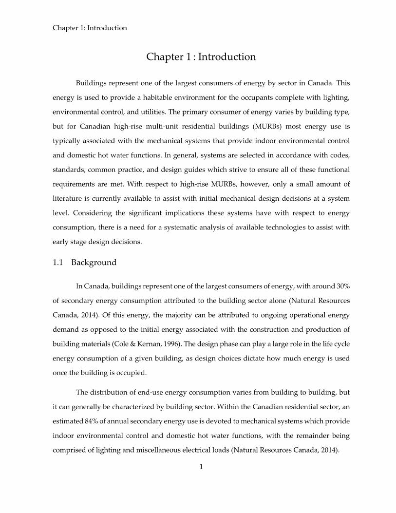
Buildings represent one of the largest consumers of energy by sector in Canada. This
energy is used to provide a habitable environment for the occupants complete with lighting,
environmental control, and utilities. The primary consumer of energy varies by building type,
but for Canadian high-rise multi-unit residential buildings (MURBs) most energy use is
typically associated with the mechanical systems that provide indoor environmental control
and domestic hot water functions. In general, systems are selected in accordance with codes,
standards, common practice, and design guides which strive to ensure all of these functional
requirements are met. With respect to high-rise MURBs, however, only a small amount of
literature is currently available to assist with initial mechanical design decisions at a system
level. Considering the significant implications these systems have with respect to energy
consumption, there is a need for a systematic analysis of available technologies to assist with
early stage design decisions.
1.1 Background
In Canada, buildings represent one of the largest consumers of energy, with around 30%
of secondary energy consumption attributed to the building sector alone (Natural Resources
Canada, 2014). Of this energy, the majority can be attributed to ongoing operational energy
demand as opposed to the initial energy associated with the construction and production of
building materials (Cole & Kernan, 1996). The design phase can play a large role in the life cycle
energy consumption of a given building, as design choices dictate how much energy is used
once the building is occupied.
The distribution of end-use energy consumption varies from building to building, but
it can generally be characterized by building sector. Within the Canadian residential sector, an
estimated 84% of annual secondary energy use is devoted to mechanical systems which provide
indoor environmental control and domestic hot water functions, with the remainder being
comprised of lighting and miscellaneous electrical loads (Natural Resources Canada, 2014).

Chapter 1: Introduction
2
High-rise multi-unit residential buildings – also known as multifamily buildings in the
United States – represent a small but growing percentage of the Canadian building stock. Often
referred to as apartment or condo buildings, MURBs of more than 75 feet in height
(approximately 6 stories) are classified as high-rises (International Code Council, 2014). As of
2011, high-rise MURBs represented 9% of the Canadian occupied residential building stock
based on number of dwelling units. This housing segment showed significant growth between
1991 and 2011 and this growth is expected to continue as cities increase in population density
(Canadian Mortgage and Housing Corporation, 2012). MURBs pose unique design challenges,
with many recurring problems becoming apparent to the engineering community over the past
30 years – particularly with respect to thermal comfort and indoor air quality, but also in terms
of energy consumption.
A small amount of literature is currently available to assist with initial design decisions
surrounding mechanical systems in high-rise MURBs. Generally, relevant expertise is held
within consulting firms and is developed through years of industry experience with this
building type. As such, without direct industry contact it is difficult to ascertain what current
practices are, or the relative advantages and disadvantages of different designs at a system
level. Most standard practices have developed during a time when energy efficiency was not
highly valued, low capital cost was the primary driver, and target demographics for the
buildings were different than at present. Furthermore, any change from conventional, proven
systems brings with it inherent risk that the new system may not function as intended, as well
as additional learning required by all levels of personnel involved with the design and
construction process. This risk and learning curve combine to generally increase the budget
required to implement unproven systems. Consequently, there are obstacles to innovation and
a tendency towards conventional solutions.
1.2 Objectives
This research seeks to answer the following question: with respect to the range of
climates in Canada, and given currently available technologies, which mechanical systems are

Chapter 1: Introduction
3
best suited for use in high-rise MURBs? In this context, best refers to a combination of economic,
environmental, and physical system characteristics.
The objective of this thesis is to systematically evaluate and compare mechanical
systems in Canadian high-rise MURBs with an emphasis on energy consumption, operating
costs, and carbon emissions in order to identify the most appropriate system selections under
varying conditions. This thesis also aims to contribute to the available literature associated with
the early stage design of said systems. Specifically, the goals are as follows: (1) develop a
baseline computer model of a typical of current construction practices from measured field
data, (2) generalize the model to reflect current practices in three different Canadian locations,
(3) simulate a set of different mechanical systems based on currently available technologies,
and (4) systematically compare systems based on design choices and stakeholder priorities in
order to identify the most appropriate options for new MURBs. Based on the results of these
simulations, this work aims to draw conclusions and make recommendations with respect to
the design of mechanical systems for new high-rise MURBs in Canada.
1.3 Scope
This research is only concerned with indoor environmental control and domestic hot
water systems, and does not address domestic cold water systems, sanitary systems, sprinkler
systems, elevators, or any other systems typically designed by the mechanical consultant on a
residential building project.
The systems in question are only considered with respect to selected Canadian climates.
More specifically, three key cities with varying climate types are analyzed but the results may
be extrapolated to other parts of North America with similar climates. The three cities chosen,
Vancouver, Edmonton, and Toronto, cover a range of different Canadian climate zones.
The analysis is limited to high-rise non-combustible multi-unit residential buildings
greater than 6 stories in height. In this case, non-combustible construction is defined as steel
and concrete structural assemblies. Furthermore, only new construction projects are

Chapter 1: Introduction
4
considered, although deep energy retrofit projects which result in significant enclosure
enhancements and total replacement of mechanical systems can often be considered similar to
new construction.
Mechanical system design discussions are limited to an early stage context, and do not
address detailed designs or specifications.
Energy consumption is analyzed on a detailed quantitative basis, but all practical
characteristics including economic and comfort characteristics are analyzed on a qualitative
basis.
Further limitations are imposed by simplifying assumptions associated with the
modelling inputs, often informed by building standards such as ASHRAE Standard 90.1 or
energy modelling guidelines such as the Model National Energy Code of Canafda for Buildings
(MNECB).
1.4 Methodology
Comparing mechanical system energy consumption would ideally be conducted
experimentally with monitoring and utility data from a set of existing buildings located across
Canada. However, this kind of an experimental setup would be costly, time consuming, and
would generate a very large amount of data which would be difficult to collect and analyze.
Building energy simulation software provides a lower cost, faster, and more flexible means of
performing this analysis.
Modern energy simulation or energy modelling software calculates an energy balance
at sequential time steps – often hourly increments over a typical year – on a computer model of
a given building in order to determine both space and system loads. Many different software
packages are available with different calculation engines and modelling capabilities.
DesignBuilder is the energy modelling software selected for this project. DesignBuilder
consists of a third-party user interface built on top of the open source platform of EnergyPlus
(DesignBuilder Software, 2008). EnergyPlus was developed by the US Department of Energy

Chapter 1: Introduction
5
(DOE), and is the most recent in the line of DOE energy modelling software packages.
EnergyPlus uses the heat balance method at incremental time steps, which is generally accepted
as being more accurate than previous calculation methods such as the radiant time series or bin
method (Hanam, 2010). EnergyPlus can be difficult to interact with directly, however, which is
why third-party interfaces are frequently used. All analyses in this thesis use DesignBuilder
version 4.6.0.015 and EnergyPlus version 8.4.001.
The energy modelling analysis is conducted in two phases. The initial phase consists of
modelling an existing high-rise MURB about which abundant design and operational data is
available. This serves to help identify key design characteristics inherent to high-rise MURBs
while also serving as a verified baseline for future simulations. In the second phase, three
reference buildings are developed by modifying the baseline model to be consistent with
building codes and typical practices in Vancouver, Edmonton, and Toronto. A further three
reference buildings are added to represent more expensive and higher performance
construction technologies based on literature. All six reference buildings are then used to
simulate different mechanical systems and compute the associated energy consumption,
operational costs, and greenhouse gas emissions.
Based on the modelled mechanical systems, comparisons and observations can be made
within climate zones with respect to energy consumption while also addressing economic,
environmental, and physical system characteristics not captured by the energy model. From
this assessment, conclusions can be drawn and recommendations formed with respect to
mechanical system selections for low-energy high-rise MURBs.
1.5 Literature Review
Currently available literature relevant to mechanical systems in high-rise multi-unit
residential buildings falls into three broad categories: discussions of whole building energy
consumption, design documentation and analysis reports, and performance issues in existing
buildings. A critical review of each category is provided below.

Chapter 1: Introduction
6
1.5.1 Energy Use in High-rise MURBs
In recent years, awareness of energy consumption has sparked a series of broad
initiatives to better understand how energy is currently being used. With respect to buildings,
a number of jurisdictions (e.g. New York City, European Union) have begun to require public
disclosure of energy consumption, with many academics, research groups, and consultancies
producing reports quantifying how the current building stock uses energy and identifying
ways in which efficiency can be improved. As comparing energy numbers alone often has
limited application, normalized metrics such as energy use intensity (EUI, defined as energy
use per unit conditioned floor area) and energy per dwelling unit are often used (Kohta Ueno,
2010a). As high-rise MURBs have been the focus of some studies and jurisdictions, there is a
considerable amount of available high-level literature discussing the energy use of this building
type.
RDH Building Engineering (RDH), a consultancy, released a 2012 report focused on
energy benchmarking of high-rise MURBs located in the lower mainland of British Columbia
(RDH Building Engineering, 2012). The study was based on utility data from 39 high-rise
MURBs. They reported average annual energy use intensity of 213 ekWh/m2, with 37% of this
energy being used for space conditioning. While the purpose of the study was aimed at building
enclosure energy efficiency strategies, some evaluation of mechanical systems was also
conducted. It was concluded that decoupling the space conditioning and ventilation systems
improves efficiency and traditional pressurized corridor ventilation systems do not provide
adequate ventilation. The study also concluded that separate in-suite ventilation and space
heating strategies could lead to improved energy efficiency and system efficacy, with heat
recovery ventilators showing significant energy savings.
A study by the University of Toronto focused on energy benchmarking and
characteristics of MURBs in the City of Toronto (Touchie, Binkley, & Pressnail, 2013). Their
refined dataset consisted of 40 buildings with an average energy use intensity of 300 ekWh/m2.
The focus of the study was to determine building characteristics which correlate with energy

Chapter 1: Introduction
7
consumption across the dataset, and did not specifically consider mechanical systems. The
study did however conclude that MURB energy use correlated with boiler efficiency.
Liu conducted a study with some of the same data as Touchie et al. by using the CMHC
HiStar database (Liu, 2007). In total, 81 Canadian MURBs were analyzed with respect to their
energy consumption and energy intensity. Across Canada, the average EUI was 0.96 GJ/m2 (267
ekWh/m2) with Ontario high-rises at 0.94 GJ/m2 (261 ekWh/m2). General trends were found
between location and EUI, likely due to varying climates. West Coast MURBs used the least
energy, and those in the Prairies used the most, although most of the sample buildings were
located in Ontario.
Seattle implemented mandatory energy benchmarking in 2010, and has compiled
results of over 3000 buildings – more than half of which were classified as multifamily (Seattle
Office of Sustainability & Environment, 2015). The average high-rise multifamily building
consumed 155 ekWh/m2 (49 kbtu/ft2), which was substantially higher than low- and mid-rise
MURBs. This finding was based on 90 high-rise MURBs, which were defined as buildings of 10
or more stories. Additionally, with respect to building age, modern multifamily buildings were
found to have the highest energy use intensities since 1950s era construction. Furthermore, both
the energy use intensity and energy use per dwelling unit were found to increase with the
number of floors. It was suggested that this can be attributed to the higher glazing ratios of
most high-rise MURBs, but it could also be associated with additional distribution losses and
more complex mechanical systems.
The Canadian Mortgage and Housing Corporation (CMHC) conducted a study of
strategies to achieve low-energy MURBs in different Canadian climate regions (Canadian
Mortgage and Housing Corporation, 2015). In this context, low-energy was defined as
achieving the Canadian Passive House standard which requires very low heating and total
primary energy intensities of 15 ekWh/m2 and 120 ekWh/m2 respectively, as well as high levels
of airtightness. The study found that based on currently available enclosure technologies, it is
possible to achieve compliance with this standard in Vancouver and Kelowna with a high
performance enclosure, electric baseboards and in-suite heat recovery ventilators. Furthermore,

Chapter 1: Introduction
8
the low-energy model buildings using electric heating were not found to be economically viable
in locations where the ratio between the cost of electricity and natural gas was greater than 4,
such as Toronto or Edmonton.
1.5.2 Design of Mechanical Systems for High-rise MURBs
Heating, ventilation, air conditioning and domestic hot water equipment is generally
well understood and documented within the industry. However, different building types and
applications often require different systems and design approaches. For this reason, many
common building types such as hospitals, laboratories, or core and shell commercial
construction have their own design guides. High-rise multi-unit residential buildings do not
have a dedicated publicly available design guide, or even documentation of current practices.
As such, only limited relevant literature is currently available to assist with the design and
system selection process.
A commonly cited authority on mechanical design of building systems in North
America is the American Society of Heating, Refrigeration, and Air Conditioning Engineers
(ASHRAE). ASHRAE maintains a series of four handbooks intended to cover the basics of
mechanical building design, with supplemental design guides and research papers available to
provide additional insight when needed. Despite the popularity of the building type, no design
guide exists for high-rise MURBs. Additionally, the HVAC Applications handbook, while
intended to cover all common building types, contains only limited information on high-rise
MURBs (American Society of Heating Refrigerating and Air-Conditioning Engineers, 2015).
This information is spread between three chapters: residences, tall buildings, and hotels, motels,
and dormitories.
The 2015 ASHRAE Handbook of HVAC Applications does address high-rise MURBs,
but only briefly in a one page subsection of the chapter on residences (American Society of
Heating Refrigerating and Air-Conditioning Engineers, 2015). The section does mention some
common HVAC systems and equipment including hydronic four-pipe fan coils, water loop heat
pumps, packaged terminal heat pumps (PTHP) and air conditioners (PTAC), and unitary forced

Chapter 1: Introduction
9
air furnaces. A small amount of design guidance and system selection criteria is provided,
although in some cases further information can be found in the Systems and Equipment
handbook (American Society of Heating Refrigerating and Air-Conditioning Engineers, 2012).
Specific challenges associated with apartment buildings are also identified such as the
difficulties related to controlling infiltration and ensuring adequate indoor air quality, and the
internal gains associated with distribution losses from domestic hot water piping. The chapter
on tall buildings in the HVAC Applications handbook includes a discussion of stack effect and
wind pressure which is relevant to high-rise MURBs, but the HVAC discussions are all focused
on commercial construction and largely are not applicable. The chapter on hotels, motels, and
dormitories is somewhat relevant as well in that multiple dwelling units are present within one
structure, but the internal gains, operation schedule, and design priorities of these buildings are
quite different than those present in high-rise MURBs.
The Canadian Mortgage and Housing Corporation published a guide to mechanical
equipment within low-rise MURBs in 2001. While no comparative analysis was conducted, the
guide does provide a list of pros, cons, capital costs, operational costs, and general energy
performance characteristics associated with an exhaustive list of mechanical equipment
typically found in low and high-rise MURBs (Canadian Mortgage and Housing Corporation,
2001). Furthermore, the guide focuses on individual pieces of equipment rather than systems
containing combinations of equipment working together, and does not form any design
recommendations.
Building Science Corporation (BSC) has published a series of papers on various building
science topics – several of which are relevant to the mechanical design of MURBs. Lstiburek
assembled a list of recommendations for HVAC systems in multi-unit residential buildings
which puts an emphasis on compartmentalization of the ventilation system along with the
heating, cooling, and domestic hot water systems such that each unit is essentially treated as a
separate detached house (Lstiburek, 2006). The motivation behind these design decisions is
based on practical industry experience with respect to maintenance issues, operational costs,
capital costs, and ensuring adequate indoor air quality. Similar arguments are made by Straube

Chapter 1: Introduction
10
in more general discussions of best practices for HVAC systems with respect to balanced
ventilation and compartmentalization (J. Straube, 2009).
RDH in conjunction with Walsh Construction Co. (WCC) completed a report in 2005
focusing on practical industry based recommendations for mechanical systems in MURBs
located in the Pacific Northwest (RDH Building Sciences, 2005). No quantitative analysis was
conducted, but experience-based qualitative guidelines and recommendations were provided
– largely aimed at ensuring building durability and delivering reliable indoor air quality. WCC
took these recommendations a step further in 2011, adding additional low-energy targets which
they quantified with energy modeling and life-cycle costing (Walsh Construction Co., 2010,
2011). WCC did not conduct extensive energy modeling however, and relied on loads generated
by a single suite eQuest model of a hypothetical building.
1.5.3 Documented Performance Issues in Existing Buildings
High rise multi-unit residential buildings have been present within the Canadian
building stock for quite some time. While each building is different, some recurring
performance issues are prevalent, and are consequently well studied by the building design
community. The most notable issues are associated with inadequate indoor air quality, and are
typically related to mechanical ventilation or infiltration. Many papers provide recommended
alternatives, but despite all of this literature, practices have remained unchanged in most
Canadian jurisdictions.
The Canadian Mortgage and Housing Corporation published a study in 2003 which
evaluated ventilation systems specifically for Canadian MURBs with the purpose of assessing
current practices and developing innovative alternatives (Canadian Mortgage and Housing
Corporation, 2003). The study identified numerous issues with conventional MURB ventilation
systems revolving around their inability to ensure adequate indoor air quality. The study went
on to evaluate alternatives to conventional systems with a focus on heat recovery for energy
efficiency and balanced air flow control for indoor air quality. Both proved to be important
design considerations in terms of system efficacy, efficiency, capital cost, and operational cost.

Chapter 1: Introduction
11
The Consortium for Advanced Residential Buildings (CARB) performed a number of
different airflow measurement tests on mechanical ventilation systems in MURBs located
largely in the Northeastern US in order to evaluate current ventilation strategies (Maxwell,
Berger, & Zuluaga, 2014). While meeting make-up air (MUA) requirements is important, an
interesting finding was that many systems do not provide make-up air through controlled
means. Make-up air through ducted supply from a central air handling unit was found to
provide the most reliable controlled MUA with 71.4% through controlled means. All the other
systems tested performed much more poorly, including those with pressurized corridor
systems, passive trickle vents, and PTAC units. In all cases, the performance of the system
varied widely from suite to suite and building to building, often with design flow rates vs.
airflow measured ranging from less than 50% to more than 150%. For high-rise MURBs, ducted
make-up air from central air handling units was recommended.
Handegord described an alternative approach to corridor pressurization ventilation
systems based on experience and observation of current deficiencies (Handegord, 2001).
Specifically, pressurized corridor systems were found to violate ASHRAE recommendations,
building codes, and provide inadequate smoke, sound, and airflow control. The alternative
system proposed would involve compartmentalized suites with in-suite exhaust and passive
inlet supply air. With induced passive supply through the enclosure, condensation concerns
can be eliminated in heating dominant climates such as Toronto. Additionally, airflow and
smoke control could be improved given the elimination of vertical duct runs or door undercuts
for supply air.
Ricketts conducted a field monitoring study of a high-rise MURB located in Vancouver,
British Columbia, both pre- and post- building enclosure rehabilitation (Ricketts, 2014). The
focus of the study was on airflow and ventilation with an emphasis on understanding airflow
characteristics rather than on the mechanical systems explicitly. The study did, however,
conclude that pressurized corridor ventilation systems fail to consistently provide adequate
ventilation air, over ventilating upper floor suites and under ventilating lower floor suites, and
consequently do not constitute a viable ventilation strategy regardless of energy consumption.

Chapter 2: Residential Mechanical Systems and Equipment
12
Chapter 2 : Residential Mechanical Systems and Equipment
A mechanical system is a very broad term which encompasses all systems inherent to
building design that move mass or thermal energy. This typically includes heating, ventilating,
and air conditioning (HVAC) systems, plumbing and drainage systems, and fire protection
systems, but may also include any other system meeting the previous definition. This chapter
serves to provide background information surrounding mechanical systems which are
responsible for substantial portions of whole building energy use in high-rise MURBs.
Specifically, an understanding of mechanical functions and characteristics will be developed
and then applied first at an equipment level and then at a system level. Note that background
information on energy use in buildings can be found in Appendix A.
2.1 Energy Intensive Mechanical Systems
In residential buildings, annual energy consumption is primarily attributed to
mechanical systems, with the remaining energy associated with lighting and miscellaneous
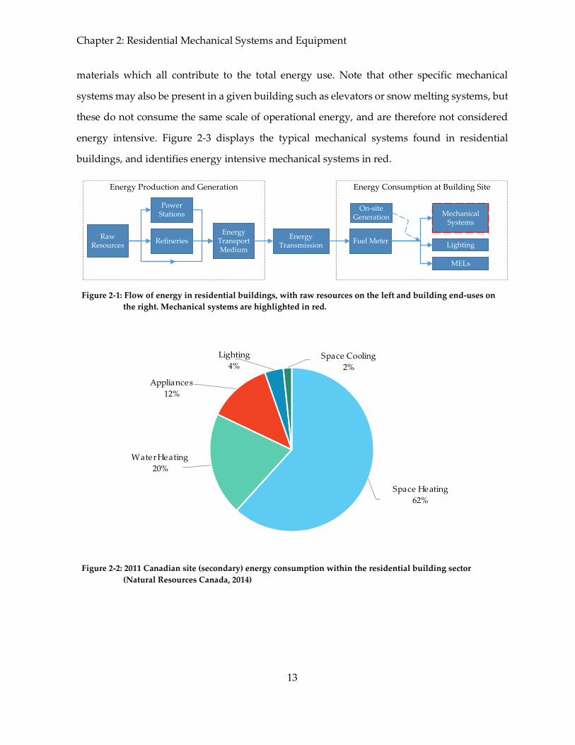
electrical loads (MELs). Figure 2-1 shows the flow of energy use in buildings from the raw
resources to the building end-uses, and illustrates the concept of source-to-site energy. Within
Canadian residential buildings, specific mechanical systems tend to dominate national
consumption as shown in Figure 2-2 (Natural Resources Canada, 2014). While many other
mechanical systems may present in a typical residential dwelling, space heating and water
heating are the major end-uses within the sector.
Space heating and water heating both describe individual energy uses or functions, but
do not describe the overarching parent systems of which they are associated. Space heating is
one function within the parent grouping of indoor environmental control systems (IECS), and
may exist independently or coupled with other IECS (J. F. Straube, 2014). Similarly, water
heating is one function within plumbing and drainage systems, and may exist as an
independent domestic hot water (DHW) system, or coupled with other systems. Both complete
space heating and water heating systems involve some combination of equipment and
Chapter 2: Residential Mechanical Systems and Equipment
13
materials which all contribute to the total energy use. Note that other specific mechanical
systems may also be present in a given building such as elevators or snow melting systems, but
these do not consume the same scale of operational energy, and are therefore not considered
energy intensive. Figure 2-3 displays the typical mechanical systems found in residential
buildings, and identifies energy intensive mechanical systems in red.
Power Stations
RefineriesRaw
Resources
Energy Transport Medium
Energy Production and Generation
Energy Transmission
Energy Consumption at Building Site
Mechanical Systems
Lighting
MELs
Fuel Meter
On-site Generation
Figure 2-1: Flow of energy in residential buildings, with raw resources on the left and building end-uses on
the right. Mechanical systems are highlighted in red.
Figure 2-2: 2011 Canadian site (secondary) energy consumption within the residential building sector
(Natural Resources Canada, 2014)
Space Heating
62%
Water Heating
20%
Appliances
12%
Lighting
4%Space Cooling
2%

Chapter 2: Residential Mechanical Systems and Equipment
14
Mechanical Systemsin Residential Buildings
Indoor Environmental Control Systems (HVAC)
Fire Protection SystemsPlumbing and Drainage
SystemsOther
Domestic Hot Water Heating and Supply
Domestic Cold Water Supply
Sanitary Water Removal
Heating Cooling Ventilation Humidification/
Dehumidification Air Filtration Pressure and Air
Flow Control
Sprinklers Standpipes Fire Dampers/ Smoke
Control
Elevators Escalators Snow Melting Etc.
Figure 2-3: Mechanical systems in residential buildings with energy intensive mechanical systems
highlighted in red
Indoor environmental control systems is a term used to describe systems which provide
a comfortable and healthy environment for occupants residing within a building (J. F. Straube,
2014). This includes heating, cooling, ventilation, humidification, dehumidification, air
filtration, and air flow control. The areas within the building which are serviced by the IECS
are collectively referred to as conditioned space, and are often broken down into individual
zones within the building. In this context, a zone is a location with uniform IECS loads, as
defined by a physical area or volume. The term “HVAC” is a common industry acronym and
colloquially refers to the same systems as IECS. The acronym itself, however, refers specifically
to heating, ventilation, and air conditioning which is somewhat limiting, and therefore will not
be used much within this discussion.
Plumbing and Drainage systems encompass all of the systems and equipment
associated with the conditioning and supply of hot and cold water for cleaning and general
purpose use, along with the piping required to capture and dispose of the wastewater to the
municipal infrastructure. Domestic hot water systems are commonly abbreviated to DHW and
comprise the equipment required to heat and store the hot water along with the pipes and
pumps required to deliver it to the required locations throughout the building. DHW systems
use considerably more energy than domestic cold water or wastewater systems as they must
heat the water in addition to transporting it.

Chapter 2: Residential Mechanical Systems and Equipment
15
Fire protection systems, as the name implies, are associated with the control and
prevention of fires which occur within buildings. These systems are strictly defined in fire safety
and building codes as they deal directly with the protection of human life – the primary
responsibility of all engineered systems. Sprinkler systems contain pressurized water at all
times with temperature sensitive sprinkler heads which release water in the event of a fire in
an attempt to prevent the spread of fire. Fire dampers are temperature sensitive louvers which
can close off a duct to airflow in the event of a fire. Standpipes act like fire hydrants and are
located near the entrances of buildings so that firefighters can attach their fire hoses to them for
supply.
Other mechanical systems, such as elevators, are designed, built, and installed by
specific consultants which deal only with one given system. A general mechanical consultant
will often not have any involvement with the design of these systems.
Energy intensive mechanical systems comprise the majority of mechanical energy use
in residential buildings, along with significant associated operational and maintenance costs.
In addition, unlike fire protection systems which are tightly prescribed by fire safety codes,
energy intensive mechanical systems are highly variable as many system options and
equipment types exist and are permitted by building codes. As such, the capital and operational
costs as well as the energy consumption of these mechanical systems is largely impacted by the
mechanical design process.
2.2 Functions of Energy Intensive Mechanical Systems
Energy intensive mechanical systems have been identified as those which address
indoor environmental control and domestic hot water functions. However, the design process
always starts by identifying the problem to be addressed which can be referred to as the design
intent. For domestic hot water systems, the goal is clearly to provide potable hot water to
designated spaces within each dwelling unit. In the context of indoor environmental control
systems, the problem consists of maintaining an indoor environment which may be different
Chapter 2: Residential Mechanical Systems and Equipment
16
than the local outdoor environment. Specifically, the goal is to maintain acceptable thermal
comfort and indoor air quality within the interior space.
Thermal comfort is a broad term which refers to a handful of different criteria. It
identifies conditions which satisfy a statistically acceptable portion of the population with
respect to the air temperature, mean radiant temperature, humidity, and air velocity. It is a
heavily studied research area, and consequently is addressed by dedicated standards such as
ASHRAE Standard 55 (American Society of Heating Refrigerating and Air-Conditioning
Engineers, 2013).
Indoor air quality (IAQ) refers to the concentrations of particles and gaseous
contaminants found in interior air. As such, acceptable indoor air quality implies these particles
and contaminants are within established safe ranges for human occupancy. In building
applications, the practical solution to provide acceptable IAQ involves reducing or eliminating
pollutant sources, direct exhaust of pollutants, and dilution of remaining pollutants with clean
air often from outdoors. These general strategies can include filtration, air cleaning, humidity
control, and airflow control. ASHRAE Standard 62.1 is frequently referenced by North
American building codes, and establishes minimum acceptable ventilation rates and
contaminant ranges (American Society of Heating Refrigerating and Air-Conditioning
Engineers, 2016).
Design functions describe the tasks which must be accomplished by the design in order
to solve the problem and thus meet the design intent. Unlike thermal comfort and indoor air
quality, which are broad terms, design functions are specific and tangible requirements.
Mechanical systems may be required to address up to seven functions in order to meet the
design intent:
1. Heating
2. Cooling
3. Ventilation
4. Filtration and air cleaning
5. Humidification and dehumidification

Chapter 2: Residential Mechanical Systems and Equipment
17
6. Air pressure and airflow control
7. Domestic hot water
Heating, or space heating, refers to the addition of heat to conditioned interior space in
order to maintain an interior temperature setpoint. The temperature setpoint typically is based
on occupant thermal comfort, but in special circumstances can also serve to satisfy thermal
energy storage requirements for objects or building materials within conditioned space. In
Canada, some form of heating is required in all occupied residential buildings.
Cooling refers to the removal of heat from conditioned interior space in order to
maintain an interior temperature setpoint. As with heating, the temperature setpoint is based
on occupant thermal comfort and material requirements. In Canada, cooling in high-rise
MURBs is only common in certain locations such as Toronto, but its use is becoming more
common.
Ventilation refers to the supply of clean air, and the exhaust of indoor air in order to
remove or dilute contaminants generated within conditioned space. Typical contaminants
include carbon dioxide and water vapour from human respiration and perspiration, cooking
and waste odours, and off gassing of objects and building materials within the space.
Ventilation can be provided passively, but often requires an active mechanical solution.
Filtration and air cleaning refers to the removal of particulates and gaseous
contaminants from air within conditioned space in order to keep concentrations within
acceptable levels. Some level of filtration is always required for equipment maintenance and
the removal of dust and allergens, but more substantial filtration and air cleaning may be
required by individuals suffering from respiratory illnesses, or if the outdoor air itself does not
meet IAQ requirements.
Humidification and dehumidification may be required in order to maintain the interior
relative humidity within an acceptable range for thermal comfort – typically 20-70% depending
on activity levels and the time of year (McQuiston, Parker, & Spitler, 2005). As with heating and
cooling, the need for humidity control is dependant on the climate, and thus is of varying

Chapter 2: Residential Mechanical Systems and Equipment
18
importance across Canada. In a marine climate such as Vancouver, humidity control is not often
required in summer whereas in a climate such as Toronto, both humidification and
dehumidification are often desirable.
Air pressure and airflow control refers to the manipulation of relative pressure
differentials across interior and exterior partitions to influence the passive flow of air. Some
level of air pressure control is necessary to reliably provide ventilation, but often additional
requirements are imposed in order to meet other practical needs such as acoustic requirements,
odour isolation, fire and smoke control, and thermal comfort.
Domestic hot water refers to hot water which is provided for sanitary or cooking
purposes within designated spaces such as bathrooms and kitchens. While viewed as an
amenity, Canadian building codes require the provision of domestic hot water within dwelling
units when available. In the context of high-rise MURBs in major Canadian cities, DHW will
always be required.
2.3 System Characteristics
Every system can be evaluated based on a set of quantitative and qualitative criteria
herein referred to as system characteristics. The emphasis of this analysis is on the energy
consumption of each system, but this cannot be evaluated independently as many other factors
are important when comparing system design choices. System characteristics can be broken
down into three broad categories: economic, environmental, and physical, as summarized by
Figure 2-4.
Economic system characteristics are associated with the capital and operational costs of
each system. Capital costs include the initial procurement costs for each piece of equipment,
along with the initial installation and commissioning costs. Operational costs represent the
ongoing expenses associated with running the system, and include energy costs, maintenance
and repair costs. Energy costs are a function both of energy consumption as well as fuel type

Chapter 2: Residential Mechanical Systems and Equipment
19
and energy source. Maintenance costs are related to the relative ease at which maintenance can
be performed, as well as the frequency at which it is required.
Mechanical System Characteristics in Residential Buildings
Economic PhysicalEnvironmental
Release or production of contaminants in the air, water, or soil in and around the building
Energy consumption Greenhouse gas (GHG)
production
Capital costs Maintenance costs Operational / energy costs Replacement costs Return of Investment (RoI)
and life cycle analysis
Frequency and complexity of maintenance
Occupant involvement in maintenance
Complexity of controls Floor space consumed within
each suite Ceiling space consumed within
each suite (reflected ceiling plan)
Acoustics Aesthetics
Figure 2-4: Mechanical system characteristics in residential buildings (Bhatia, 2012; RDH Building Sciences,
2005)
Environmental system characteristics are associated with a given system’s interaction
with the local and global environment. The local environment includes areas within the
building, as well as areas directly surrounding the building. Factors affecting the local
environment could include the release or production of contaminants which are introduced
into the air, soil, or water at the building location. The global environment is more concerned
with larger implications such as energy consumption – and by extension, greenhouse gas
emissions.
Physical system characteristics represent the implications of each system with respect
to the space within the building, and the interaction each system has with the occupants. This
includes the frequency at which maintenance is required, the skill level required to perform
said maintenance, and the involvement necessary on the part of the occupants in conducting
this maintenance. Physical characteristics also include the means through which the occupants

Chapter 2: Residential Mechanical Systems and Equipment
20
control the system, as the well as the space consumed within each suite and the noise produced
by the operation each system.
2.4 Mechanical Equipment and Components
Every mechanical system is comprised of one or more distinct components. Some
components are very complicated and contain many pre-manufactured systems and controls,
while other components are very simple and contain no moving parts. Every component in a
mechanical system can be classified into one of the following four categories: energy
production/rejection components, distribution components, terminal units, or packaged units
(Bhatia, 2012). Figure 2-5 displays some typical components which can be found in each
category.
Energy Transport Medium
Distribution ComponentsEnergy Production/Rejection
ComponentsTerminal Units
Furnace Boiler Heat Pump Chiller Cooling Tower Air Handler HRV and ERV Refrigerant Split Unit
(evaporator or condenser)
Instantaneous / Tankless Water Heaters
Electricity Natural Gas Oil Biomass Etc.
Ductwork Piping Pumps Fans
Fan Coils (2-pipe, 4-pipe)
Radiant Panels Radiators and
Convectors Air grilles and diffusers Refrigerant Split Unit
(condenser or evaporator)
Faucets, Shower heads, etc.
Packaged Terminal Units
PTAC PTHP Baseboard and Cove
Heaters
Supply
Return
Figure 2-5: Classification of common equipment and components found in residential mechanical systems in
Canadian high-rise MURBs
Energy production/rejection components are pieces of equipment which perform an
energy conversion in order to produce or reject heat. Typically, these components are not
located in the zone which they serve, or they serve multiple zones. In either case, distribution
components are required to transport the given service from the energy production/rejection

Chapter 2: Residential Mechanical Systems and Equipment
21
component to the zone in which it is required. Once there, terminal units are required in each
zone in order to control the delivery of the service to the zone.
Although not always required, both supply and return distribution components are
often included as part of balancing and controlling the given service within the zone.
Additionally, in some cases there are multiple energy production/rejection components
connected to each other via distribution components in order to provide a given system
function or set of functions.
Packaged terminal units often contain some combination of energy production/rejection
components and distribution components, and must contain a terminal unit. By virtue of their
terminal unit inclusion, they are located within the zone they serve and are purchased as self-
contained prefabricated units.
Together, some combination of energy production/refection components, distribution
components, terminal units and packaged units can be assembled into systems which provide
the necessary functions described in Section 2.2 in each zone which they are required.
2.5 Mechanical Systems
Residential mechanical systems are typically named based on the primary function they
perform, and fall into three categories: heating and cooling systems, ventilation systems, and
domestic hot water systems. Like the acronym HVAC, this traditionally naming scheme can be
a bit misleading as the first two system categories could provide one or more additional
functions such as filtration or humidity control which are otherwise not mentioned. Therefore,
the names used to discuss said systems in this thesis will be thermal comfort systems, indoor
air quality systems, and domestic hot water systems. Figure 2-6 depicts these three systems,
and demonstrates how they are not necessarily independent but can in fact be combined into
more complex systems. The numbering of the different areas will be important for defining
systems in Section 4.2 (Test Set of Mechanical Systems) and Appendix E.

Chapter 2: Residential Mechanical Systems and Equipment
22
Thermal comfort systems, indoor air quality systems, and domestic hot water systems
are all very common and often exist independently of one another. Within each system
category, there are several subcategories based on the specific functions provided, which are
summarized in Table 2-1. Note that each subcategory is named simply after the primary
function or functions that are provided. Combination systems can straddle multiple
subcategories, but typically constitute some combination of type 1 and type 2 or type 1 and type
3 systems.
1. Thermal Comfort Systems
2. Indoor Air Quality Systems
3. Domestic Hot Water Systems
Heating Cooling Humidity Control Airflow Control (Velocity)
Ventilation Filtration Airflow Control (Pressure)
Domestic Hot Water
Figure 2-6: Residential mechanical system types 1-3 as defined for the purposes of this body of work

Chapter 2: Residential Mechanical Systems and Equipment
23
Table 2-1: Residential mechanical system subcategories as defined for the purposes of this body of work
System Number Subcategory
1a Heating
1b Cooling
1c Heating and Cooling
2a Suite Ventilation
2b Corridor Ventilation
2c Suite and Corridor Ventilation
3 Domestic Hot Water
Mechanical design requires the designer to consider both the functions and system
characteristics previously discussed in order to select equipment and components which
together constitute the overall system with its associated advantages and disadvantages. In
addition to these considerations, however, there are several system level design choices which
can dictate system selection:
1. Layout
2. Controls
3. Fuel type
4. Thermal transport fluid
The system layout refers to the relative location of energy production/rejection
components, and the scale on which the system functions. Typically, systems are either
centralized or distributed. Centralized systems involve large centrally located energy
production/rejection components, with extensive distribution networks which deliver the
service throughout the entire building to every conditioned zone. Distributed systems involve
multiple equivalent components, each of which serves a portion of the conditioned zones in the
building. Floor-by-floor, suite-by-suite, and room-by-room systems are all types of distributed

Chapter 2: Residential Mechanical Systems and Equipment
24
systems, and are characterized by the size and location of the energy production/rejection
components.
Centralized systems serve more suites and hence are larger in capacity and benefit from
economy of scale with respect to equipment cost, and may in some cases have higher efficiency,
but must overcome significant distribution energy costs and physical losses. Additionally,
centralized systems provide much easier access for maintenance, however any system
downtime corresponds with a service outage for the entire building. Lstiburek, RDH and others
have argued for suite-by-suite and room-by-room systems as they often involve simpler
equipment which can be serviced by less skilled technicians, incorporate simpler control
schemes, and can ensure that the functional requirements are met for every suite (Lstiburek,
2006; RDH Building Sciences, 2005). Table 2-2 summarizes some of the common advantages
and disadvantages of centralized and distributed mechanical systems.
Table 2-2: Advantages and disadvantages of centralized and distributed mechanical systems
System Type Advantages Disadvantages
Centralized
Economy of scale in energy
production/rejection equipment
capital cost
Easy access for maintenance
Familiarity of system designs
Less in-suite equipment helps
ensure aesthetics meet
architectural design intent
Extensive distribution system
resulting in higher distribution
losses
Any system downtime constitutes a
service outage for entire building
Control systems tend to be more
complex
Distributed
Simpler equipment and control
schemes
Equipment can be service by
less skilled technicians
Suites can be
compartmentalized, ventilation
can be more easily balanced
Equipment failure only results
in a service outage for the
individual suite
Gaining access to each suite required
for any maintenance
Often more maintenance is required
on the part of the tenants
In-suite equipment consumes
valuable floor and/or ceiling space

Chapter 2: Residential Mechanical Systems and Equipment
25
Mechanical system controls range from very simple to very complex depending on the
size of the system, the number of functions being provided by the given system, the type and
quantity of sensors being used, and the number of independent zones being served. Generally
speaking, with increasing system complexity, the more difficult it becomes to ensure energy
efficiency. Additionally, systems which serve multiple zones and provide multiple functions
may struggle to ensure all requirements are met at all times. Simultaneous heating and cooling
at a system level can completely overshadow high equipment efficiencies when it comes to total
energy consumption (Ihnen, Weitner, & Donnell, 2012). As the industry moves in favour of
building automation systems (BAS) driven by direct digital controls and complex algorithms,
many industry experts recommend simplified controls to ensure functional requirements are
met (RDH Building Sciences, 2005; J. Straube, 2009).
The availability and implications of different fuel types can also play a factor on system
level choices. Electricity is always wired to every suite, but the decision to plumb natural gas to
each suite with separate sub-metering represents a significant incremental cost if not already
part of the construction budget (Mather, 2015). Additionally, the pricing and availability of fuels
can vary greatly by location which can impact economic factors such as energy costs and return
on investment while also impacting environmental factors such as greenhouse gas emissions
based on source-to-site ratio.
The thermal transport fluid is the fluid used to convey thermal energy between the
energy production/rejection component(s) and terminal units via the distribution components
in any system providing heating and or cooling. This fluid can be water, air, or refrigerant
depending on the system in question. Unlike other functions which have a predefined medium,
such as air for ventilation or water for domestic hot water, the choice of thermal transport fluid
for heating and cooling must be made carefully. Each fluid has its associated advantages and
disadvantages as highlighted in Table 2-3.

Chapter 2: Residential Mechanical Systems and Equipment
26
Table 2-3: Advantages and disadvantages of air, water, and refrigerant for use as the thermal transport fluid in
thermal comfort systems
Fluid Advantages Disadvantages
Air
As ventilation is required, some
form of mechanical ventilation
system likely already exists as
part of the building design
which can be additionally
purposed to provide heating
and cooling
Easier to achieve well-mixed air
temperatures within
conditioned space
Less skill and effort required to
produce ductwork
Ducts take up large amounts of floor
and ceiling area if sized
appropriately to minimize noise and
fluid velocity
Complete fluid flow control is much
more difficult to achieve than with
other fluids as air loops are open
The heat capacity of air is relatively
low
Moving air at higher pressure
differentials through smaller ducts is
energy intensive
Water
Piping takes up substantially
less area than ductwork
Pumps tend to be more efficient
than fans as water is considered
to be incompressible
Water has one of the highest
heat capacities of any liquid
A separate air conveying system is
still required to meet ventilation
requirements
Terminal units – with the exception
of radiant panels – take up more
suite area than air terminal units
Leaks are costlier to repair than in air
based systems
Refrigerant
Piping takes up substantially
less area than ductwork
Refrigerant acts both as the
transport medium and the
working fluid in the vapour
compression refrigeration cycle
Can only be used in split systems,
with specific mini/multi-split
terminal units
Scale of system is often limited to a
maximum of suite-by-suite,
requiring an outdoor compressor
unit for every suite
High level of skill and effort
required for piping
Leaks are costlier to repair than in air
based systems, and many common
refrigerants have significant global
warming potential
Once the mechanical system functions have been identified, the choices of layout,
control scheme, fuel type, and thermal transport fluid all represent high level mechanical
design decisions which form the structure of subsequent system and equipment selections.

Chapter 2: Residential Mechanical Systems and Equipment
27
2.5.1 Type 1: Thermal Comfort Systems
Thermal comfort systems provide heating, cooling, or heating and cooling, along with
potentially providing a combination of other functions. While fuel types and distribution
layouts varied throughout the simulations, the heating and cooling systems chosen to be
modelled generally fell into one of the following categories: electric resistance heating, in-suite
Air Handling Units (AHUs), Fan-coil Units (FCUs) and convectors, radiant panels, Packaged
Terminal Air Conditioners (PTACs) and Packaged Terminal Heat Pumps (PTHPs), and
Variable Refrigerant Flow (VRF) heat pumps.
2.5.1.1 Electric Resistance Heating
Electric resistance heating is very common in only a few areas of North America (e.g.
the Pacific Northwest), and can take on many physical forms. These include cove heating,
radiant panels, and electric furnaces (see Section 2.5.1.2), but the focus of this section will be
electric baseboard convectors as these are the most common type of residential electric
resistance heating (RDH Building Engineering, 2012). From a thermodynamic perspective, all
of these technologies are more or less equivalent in that heat is generated by passing an electric
current through a resistive medium, a process which has a thermal efficiency of 100%.
Electric baseboards offer low capital and maintenance costs due to their lack of moving
parts, combustion equipment, or distribution components. Operational costs, however, vary by
location, as do energy consumption and GHG emissions.
Electric baseboards are only capable of providing space heating and no other functions.
Units are typically located along exterior walls, under fenestrations to prevent condensation
and make up perimeter losses, with separate units for each zone served. The zonal nature of
the simple controls can allow for heating to operate only in occupied areas of a suite, which can
result in energy savings of up to 20% as compared to conditioning all interior space (US
Department of Energy, 2016).

Chapter 2: Residential Mechanical Systems and Equipment
28
Physically, electric baseboards do require space within the zones they serve, which can
negatively impact interior aesthetics and requires suite access for maintenance in the rare
occasion that it is required. The footprint of each baseboard is relatively modest, and due to the
lack of moving parts, baseboards have little impact on acoustics.
2.5.1.2 In-suite Air Handling Units
In-suite air handling units (AHUs) take the concept of forced air heating and cooling
common single-family low-rise housing, and implement it on a suite-by-suite basis in multi-
unit residential buildings. The heating technology may be a natural gas or electric furnace, or
an air or water source heat pump. In all cases, conditioned air is transported from a central unit
– typically located in a perimeter mechanical closet directly vented to the exterior – to each zone
of the suite via ductwork. While cooling is not necessarily required in these systems, the ability
to easily add cooling and other functions is one of the major advantages these systems offer
over electric baseboards or radiant floors (see Section 2.5.1.4). As such, in-suite AHUs can
provide heating, cooling, and filtration, with dehumidification occurring only during cooling
operation, and provision for humidification possible but often not included.
In practice, packaged units containing the heating and cooling equipment along with
distribution fans and filters are produced by many manufacturers. Those implementing warm
air furnaces with direct expansion cooling or air source heat pumps are completely self-
contained, and do not rely on any other plant equipment.
All in-suite AHUs require distribution ductwork to be installed throughout each suite,
although ductwork tends to be limited and simple given that most suites are compact. Even so,
ductwork can add distribution energy, duct losses, and acoustic concerns if not sized properly
(John, 2014; Zimmerman, 2013). Additionally, the throw of air terminal units must be carefully
specified to not negatively impact thermal comfort, and the placement of ducts must be
coordinated with the reflected ceiling plan of each suite.
The requirement for in-suite ductwork can lead to moderate installation costs as
compared to electric baseboards, but the total capital and maintenance costs are somewhat

Chapter 2: Residential Mechanical Systems and Equipment
29
dependant on the type of energy production/rejection equipment (US Department of Energy,
2016). Furthermore, if not already part of the budget, plumbing natural gas to each suite
represents a substantial incremental cost (Mather, 2015). Electric resistance heating, as
previously discussed, will have lower installation and maintenance costs than combustion
equipment. With added complexity, the skill level required and cost of maintenance tends to
increase, and this is even more relevant to heat pump based systems (Lstiburek, 2006).
As these units are located in conditioned space, furnaces are classified as non-
weatherised and can achieve higher efficiencies than weatherized units as jacket losses usually
provide useful heat gain to the spaces they are located in (Lutz, Dunham-Whitehead, Lekov, &
McMahon, 2004). This does however mean that proper air supply and exhaust is required for
combustion equipment, and access to outdoor air is required for heat rejection and collection
when implementing vapor compression refrigeration equipment. Properly designing the
combustion gas venting is very important to ensure proper system performance without
compromising indoor air quality (Dale, Wilson, Ackerman, & Fleming, 2000). These added
penetrations through the building enclosure are often quite large, and can create difficulties
with respect to detailing the continuity of enclosure control layers.
The overall heating and cooling efficiency of the system (based on site energy use, not
always source energy) is largely dependent on the type of energy production/rejection
equipment selected, with heat pumps offering the highest efficiencies, followed by electric
resistance heating and lastly condensing natural gas furnaces. Air source heat pumps can only
operate to a set minimum outdoor air temperature below which system performance drops off.
In the past, this temperature was high enough that most heat pump systems in cold climates
required backup electrical heating, but a growing number of systems have sufficient capacity
and efficiency to obviate the need for backup heating (Natural Resources Canada, 2015). While
the heating fuel source may be natural gas or electricity, all systems require electricity for
cooling as well as fan energy for circulation – something which can account for a non-trivial
amount of annual energy consumption (Pigg, 2003).

Chapter 2: Residential Mechanical Systems and Equipment
30
Control strategies for in-suite AHUs tend to be fairly rudimentary, with one thermostat
located in a central location, and balanced delivery of air to all zones in the suite. This limits the
ability to provide zone level control, but such control is rarely required in modestly sized suites,
and the single thermostat greatly simplifies installation, commissioning, operation, and
maintenance.
2.5.1.3 Hydronic Fan Coil Units and Convectors
Hydronic systems typically involve boilers and chillers which transport energy using
water to hydronic terminal units located within conditioned spaces. Fan coil units (FCUs) and
convectors are both examples of hydronic terminal units, and both are available in a few
different forms. Hydronic convectors can only provide heating, but fan coil units can provide
heating and cooling if energy rejection components such as chillers are incorporated into the
system design.
Fan coil units are typically 2-pipe or 4-pipe, which denotes the number of supply and
return pipes connected to each terminal unit. 2-pipe FCUs have a single supply and return, and
thus can only provide heating or cooling at one time, and require seasonal transitions between
energy production and rejection equipment if cooling is desired (American Society of Heating
Refrigerating and Air-Conditioning Engineers, 2012). It is common to have electric resistance
backup coils in 2-pipe configurations to assist in shoulder season conditions when the plant has
been transitioned to cooling but heating is required to satisfy setpoint temperatures. Four (4)-
pipe FCUs have independent supply and return piping for heating and cooling water. This
arrangement – while more capital cost intensive – is generally preferable due to eliminating the
need for seasonal transitions between plant equipment, and added ability to provide heating
and cooling to different zones at the same time during shoulder seasons. In either case, each
unit consists of a water-to-air heat exchanger and a fan, and utilizes forced convection to
condition space air.
Convectors utilize natural convection to deliver heat to a given space. As natural
convection is less effective at driving heat transfer than the forced convection achieved by the

Chapter 2: Residential Mechanical Systems and Equipment
31
fans in FCUs, convectors rely more heavily on high temperature differences between heating
water and space air, along with larger heat exchangers. As high temperate differences are more
easily achieved when heating than when cooling, and due to the requirement for condensate
drains for cooling coils, convectors are typically only used for heating.
Convectors can take the form of baseboard heaters, induction units (which require
forced air from a remote source), or radiators. Note, however, that baseboards and radiators are
the most common forms of convectors, and as convective heat transfer comprises the majority
of total heat transfer from radiators, both are essentially thermodynamically equivalent.
Hydronic systems offer many advantages over air-based systems in that they can
deliver the same amount of heat while requiring significantly less space for distribution
equipment, and while consuming substantially less distribution energy than air-based systems
due to the higher heat capacity and density of water (Boldt & Keen, 2015). The terminal units
still require space within each conditioned zone however, which can have a negative impact on
aesthetics and acoustics in the case of FCUs.
Condensing natural gas boilers can be extremely efficient, with peak thermal efficiencies
reaching 97% and beyond (Charbonneau, 2011). However, boiler efficiency is highly dependent
on entering water temperature, that is, the temperature of the water returning to the boiler from
the supply loop. With FCUs and convectors, it is common to supply water at temperatures of
70-80°C, with a loop delta T of 10-15°C. At these temperatures, regardless of the peak rated
efficiency of the boiler, condensing efficiencies will not be achieved, and the system will operate
in a non-condensing fashion with peak thermal efficiencies around 80-85%. Modern
engineering that favours energy efficiency would design systems to ensure low return water
temperatures. Reducing the water temperatures would improve boiler efficiency, and may
either require an increase in pumping energy or larger plumbing. Furthermore, lower
temperature differences between water and space air will require larger terminal units and/or
larger fans. Outdoor reset control systems for boilers account for the much lower heat demand
at warmer-than-design outdoor temperatures by lowering supply water temperatures. Such
controls can allow condensing efficiencies during the vast majority of operating hours per year

Chapter 2: Residential Mechanical Systems and Equipment
32
with no change in distribution or terminal equipment (The Viessmann Group, 2004).
Condensing efficiencies are therefore possible with FCUs and convectors if carefully designed,
but may be more expensive to achieve if larger sizes are required. Electric boilers alleviate the
boiler efficiency limitations. However, higher distribution losses will always be expected with
higher supply water temperatures.
Chillers are required if cooling is to be provided by fan coil units. There are many types
of chillers, but a common approach is to have a central water-to-water chiller which removes
heat from the closed building loop, and transfers it to an open loop connected to a cooling tower.
Chiller efficiencies vary by type, but not all chillers are applicable for use in high-rise MURBs
as each type has a limited capacity range. Centrifugal chillers offer the highest efficiencies, but
require a higher minimum load than rotary chillers which are more common in residential
settings (Natural Resources Canada, 2002).
Capital costs tend to be comparable to other centralized systems requiring distribution
pipe installation, along with plant equipment and terminal units. Maintenance costs depend on
the type of energy production/rejection components selected, but natural gas boilers and
evaporative cooled chillers typically require moderate maintenance costs due to the inherent
degradation of combustion equipment, and the water treatment required in order to prevent
scale buildup in open loops.
Controls are moderately complex, as water temperature, flow rate, and air flow rate can
be modified in order to achieve the desired amount of space conditioning. Thermostats can
control temperatures at a suite level or at a zone level depending on the system implementation,
and often work by varying the amount of water circulated through the terminal units from a
central closed loop. FCUs can also vary the fan speed, which is often controlled manually on
the unit itself.
2.5.1.4 Water Source Heat Pumps and Ducted Fan Coil Units
Water source heat pumps and ducted fan coils represent a combination of hydronic fan
coil units and in-suite AHUs; both involve a single unit, located in each suite, which distributes

Chapter 2: Residential Mechanical Systems and Equipment
33
conditioned air to zones through ductwork as with all in-suite AHUs. However, rather than
having a furnace or air source heat pump, each AHU contains a hydronic fan coil or water
source heat pump which is connected to a central plant loop. In this way, water source heat
pumps have unique characteristics.
Both systems require a central boiler plant to create hot water, however only ducted fan
coils require a chiller as water source heat pumps can transfer heat from space air into the closed
recirculation loop as long as it is maintained within a fairly flexible temperature range – a task
which can be accomplished with a cooling tower and heat exchanger (Mather, 2015). Loop
temperatures do have an impact on plant efficiencies, but both of these systems are capable of
operating at lower heating water temperatures.
Ducted fan coils require fewer units than having traditional FCUs located in every zone
served which does reduce capital costs, however the addition of supply ductwork and duct
losses must also be accounted for. Increased pressure drop from the ductwork will also increase
fan energy consumption. Water source heat pumps represent a cost premium over ducted fan
coils or traditional in-suite AHUs, but the lack of central chiller does reduce plant equipment
costs.
From an efficiency standpoint, water source heat pumps operate more like fan coil units
than air source pumps when heating because the boiler must still provide enough heat to the
hot water loop to meet the heating load. However, the ability to have more modest water loop
temperatures for heating and cooling will reduce distribution losses.
2.5.1.5 Radiant Panel Heating and Cooling
Radiant panel heating and cooling involves using very large terminal units, often
concealed in the building’s fabric, to provide space conditioning predominantly by means of
radiant heat transfer and natural convection between objects and occupants within the space.
Because of the nature of these systems, operative temperature becomes the dominant control
variable as opposed to air temperature. Furthermore, the radiant panels themselves can operate

Chapter 2: Residential Mechanical Systems and Equipment
34
at relatively low temperature differences with respect to the zone operative temperatures due
to the presence of large effective heat exchange areas.
Radiant panels can take many forms, depending on the energy source. Generally,
electric resistance heating elements or hydronic piping are imbedded into a cement screed or
topping which is set on top of a floor, wall, or ceiling structure. Metal panels suspended from,
or embedded in, the ceiling with hydronic tubing bonded to their backs, is another common
terminal unit. In all cases, insulation is required between the energy source and structure in
order to ensure heat only flows in one direction. Additionally, a low resistance, high emissivity
outer surface is necessary in order to ensure adequate radiative transfer between objects in the
space and the surface of the panel.
Radiant floors are commonly used for heating in order to take advantage of natural
convective currents. For these reasons, walls and ceilings do not function as effectively for
heating, and are mostly seen in cooling applications. Conversely, radiant floors are less
common in residential cooling applications, and are mostly reserved for large open rooms or
atriums with large glazing areas in order to directly control solar gains (Nall, 2013). The
effectiveness of radiant floors is commonly compromised by the presence of furniture and floor
coverings. Cooling slabs have the added complication that surface temperatures cannot drop
below the interior dew point in order to prevent condensation issues.
In locations where the practice of radiant heating is very established, such as Germany,
it is claimed that radiant floor heating is no more expensive than other hydronic systems such
as baseboard convectors (Olesen, 2002).
When heating, hydronic panels require relatively low supply water temperatures,
which enables high plant efficiencies when coupled with condensing natural gas boilers.
Additionally, as space mean radiant temperatures are higher, equivalent operative
temperatures can be achieved at lower air temperatures – a factor which can result in energy
savings, provided that the enclosure does not exert highly variable solar loads. However, the
surface temperature of radiant panels cannot exceed 30°C if occupant thermal comfort is

Chapter 2: Residential Mechanical Systems and Equipment
35
considered, and therefore radiant panel heating cannot provide more than approximately 100
W/m2 of space heating (Olesen, 2002). For this reason, radiant panel systems require high
performance enclosure assemblies to reach their full potential.
Physically, radiant panels do increase the depth of the assemblies which they are
incorporated into, which can be difficult given the tight restrictions on floor height typical of
high-rise MURBs. However, their concealed nature results in no visible presence within the
zones they serve, little or no acoustic impact depending on recirculation pump operation, and
generally very low maintenance required at a zone level.
Radiant panels can be controlled a number of different ways depending on whether
electric resistance or hydronic systems are implemented. Hydronic systems can implement
recirculation pumps within each zone with a constant flow central loop, or a variable flow
central loop with suite control valves to regulate temperatures. In either event, radiant panels
must accommodate the thermal storage of the mass in structure-integrated panels, which can
increase perceived thermal comfort but renders the system slow to respond to sudden changes
in space loads.
2.5.1.6 Packaged Terminal Heat Pumps and Air Conditioners
Packaged terminal units incorporate energy production/rejection, distribution and
delivery equipment into one component. Packaged terminal air conditioners (PTACs) utilize
direct expansion cooling either independently or coupled with electric resistance heating,
which is delivered to the zone via a distribution fan which may also serve as the evaporator
fan. Packaged terminal heat pumps (PTHPs) are similar, except that the vapour compression
refrigeration cycle can be reversed to provide heating. In either event, the units are typically
mounted on exterior walls of perimeter zones, and are most popular in applications where
individual zone level control is required such as hotels or residences.
PTACs provide cooling, and PTHPs also provide heating. Dehumidification can also be
provided indirectly when the space is being actively cooled. Filtration of space air is achieved

Chapter 2: Residential Mechanical Systems and Equipment
36
as well, but the level of filtration is often only sufficient to protect heat exchange surfaces, not
ensure air quality. Some systems include the supply of outdoor air as well.
Packaged terminal units require an independent unit for every zone served, which may
mean 2 or more units per suite, depending on the layout and perimeter exposure. The
performance and capacity of air source heat pumps is diminished at lower outdoor air
temperatures, and may require electric resistance backup heating in cold climates.
Capital costs are dependent on the number of units required per suite. If only one unit
is necessary, PTACs and PTHPs can be a relatively low cost solution, however as the number
of units per suite increases, the cost will become less competitive. Maintenance is fairly simple,
but does require suite access.
2.5.1.7 Variable Refrigerant Flow Air Source Heat Pumps
Variable Refrigerant Flow (VRF) heat pumps employ fan coil units sometimes combined
with an outdoor ventilation air system, connected to a central outdoor unit by means of
refrigerant piping. In small scale residential applications, VRF systems are often referred to as
ductless split systems, mini-splits, or multi-splits (Roth, Westphalen, & Brodrick, 2006). The
fundamental concept is to use refrigerant directly as the thermal transport medium, thus
turning the indoor fan coil units into evaporator or condenser coils, which can improve system
efficiency. Furthermore, if heating and cooling is required simultaneously in different zones
within the same system, heat can be transferred between spaces with very little energy input,
resulting in very high system COPs.
VRF systems can be implemented with one outdoor unit per suite, or with upwards of
20 indoor units connected to one outdoor unit – resulting in one outdoor unit for every few
floors (Goetzler, 2007).The indoor units typically are fan coils with no air supply, but air can be
provided through ducted units provided a secondary dedicated outdoor air system (DOAS) is
present. A suite-by-suite approach would offer the application of currently available residential
multi-split systems, which could simplify installation and maintenance (Lstiburek, 2006).
However, centralized systems offer better system level efficiency as the aforementioned part

Chapter 2: Residential Mechanical Systems and Equipment
37
load case where heating and cooling are required simultaneously in different zones will most
likely occur on opposite elevations of a given MURB.
VRF systems often claim better part load performance than traditional direct expansion
heat pumps due to multistage, variable speed compression and fan performance. Furthermore,
many outdoor units are better suited to low temperature operation, with some still capable of
delivering 100% of the heating capacity available at 16°C at temperatures as low as -20°C, and
operation down to -25°C (Afify, 2008). Beyond those limitations, electric resistance heating or a
supplemental natural gas heating system is required.
Capital costs for VRF systems largely depend on industry familiarity, but in North
America a cost premium of 5-20% over traditional hydronic systems can be expected (Goetzler,
2007). Maintenance costs would likely also be higher than conventional systems due to the
added complexity, and lack of widespread familiarity within the industry.
VRF systems boast very low electrical energy consumption compared to other system
options, which will have variable GHG implications depending on the electrical grid
infrastructure for the buildings location. However, there are hidden GHG implications which
must also be considered; while packaged heat pumps and chillers typically exhibit minimal
refrigerant leakage over the course of their service life, limited data is available for VRF systems.
The most comparable application utilizing large scale site-built refrigeration is grocery stores,
for which it is estimated 10-15% of the system refrigerant charge is lost annually (Baxter,
Fischer, & Sand, 1998). At these rates, even the recommended sustainable refrigerant R-410a
still poses significant GHG concerns as it has a global warming potential 1725 times that of
carbon dioxide (Afify, 2008). Other refrigerants with lower global warming potentials are
available for the same applications as R-410a such as propane (R-290) and R-123, but their
adoption is not currently widespread (Critchley, 2011; Lampugnani & Zgliczynski, 1996)
Functionally, several different forms of indoor units exist which can all be connected to
the same outdoor unit. These include exposed and concealed units, which can be wall mounted,
ceiling mounted, or suspended. Each indoor unit offers consistent zone level temperature
Chapter 2: Residential Mechanical Systems and Equipment
38
control, with some limited filtration of suite air. Due to the improved part load performance,
more consistent thermal comfort can also be achieved.
When installing VRF systems, vertical refrigerant pipe runs are limited (e.g. less than
60-150 feet for many models) which can pose difficulties for taller buildings (Afify, 2008). A
potential solution involves routing upper floor piping to roof mounted units with lower floors
routed to ground level units in the parkade or adjacent space, but this can only be applied to a
maximum of around 30 stories (Lstiburek, 2006). Outdoor units can also be hung on the side of
buildings, but this requires the architectural design to coordinate with the mechanical design.
Often for taller buildings, interstitial mechanical rooms are required, with enclosure area for
the air source condensing equipment.
2.5.1.8 Ground Source Heat Pumps
Ground source systems utilize a hydronic earth heat exchange loop coupled with some
combination of previously discussed systems to provide space conditioning. The building
systems will likely take one of the following three forms:
1. A central water-to-water heat pump connected to the ground loop providing
heating or cooling water to in-suite hydronic terminal units such as radiant
panels or FCUs
2. In-suite water source heat pumps which transfer heat directly to or from the
central ground water loop to suite air
3. A central water source VRF system coupled to the ground water loop
Earth heat exchange loops can either involve vertical bore holes or horizontal trenches.
Vertical bore holes are much more expensive, but require substantially less space and are
therefore often the only practical option for high density sites. As high-rise MURBs often are
situated in high density downtown areas, vertical bore holes are the only broadly applicable
configuration, often with the bore hole field located beneath the underground parking garage.

Chapter 2: Residential Mechanical Systems and Equipment
39
Ground source heat pumps offer the distinct advantage over air source heat pumps in
that the ground temperature does not undergo significant annual variations. Furthermore, the
earth can act as a form of thermal storage, being charged during the cooling season and drained
during the heating season. Most climate zones of Canada and the northern United States have
much larger heating loads than cooling loads, so a truly seasonally balanced system is unlikely.
However, as buildings strive for higher performance, the heating loads often drop more quickly
than the cooling loads, which means that ground loops can become more closely balanced.
Capital costs vary depending on the building systems implemented, but the drilling fees
associated with creating the ground loop are fairly significant – particularly with vertical bore
holes located beneath taller high-rise MURBs. Drilling costs vary from 5-15 US Dollars/foot
depending on the type of earth, but higher costs can be expected for harder rock – such as that
found beneath downtown Toronto (S. Kavanaugh, 1998). In some cases, the ground loop can be
treated as a district energy system, paid for by utility companies and billed monthly to condo
owners at an amortized rate over the service life of the building (S. P. Kavanaugh, 2016).
Investigations into implementation of ground loops in Toronto have demonstrated reasonable
payback periods provided cooling is functionally required (Canadian Mortgage and Housing
Corporation, 2002).
Ground loops offer higher efficiencies than air loops – particularly at lower outdoor air
temperatures – and can potentially provide energy savings of 20-50% over conventional air
source heat pumps (Cooperman, Dieckmann, & Brodrick, 2012). However, GSHPs do not
benefit from the economy of scale with respect to central plant efficiency, and tend to favour
smaller water source heat pumps (S. Kavanaugh, 1998). The project-specific and often complex
design of GSHPs requires more care than pre-packaged air source systems and hence
performance is highly dependant on the design choices made (especially with regard to pump
power, ground loop size, etc.).

Chapter 2: Residential Mechanical Systems and Equipment
40
2.5.2 Type 2: Indoor Air Quality Systems
Indoor air quality systems provide outdoor air in order to help address indoor air
quality requirements. The primary function served is ventilation, but some form of filtration,
humidity control, or air pressure control may also be addressed by these systems. All occupied
spaces, including the suites and corridors in high-rise MURBs require ventilation air, and as
such ventilation systems can address these locations with separate, independent systems or
with central combined systems. In either case, the fresh air requirements are usually based on
ASHRAE Standard 62.1. The delivery effectiveness (i.e. how well the system delivers design
airflow in normal operational conditions) varies depending on the system configuration and
has been shown to vary widely (Maxwell et al., 2014).
2.5.2.1 In-suite Heat Recovery and Enthalpy Recovery Ventilators
Heat recovery ventilators (HRVs) and enthalpy recovery ventilators (ERVs) are
packaged residential units which serve to provide balanced flow of ventilation air similar to a
commercial dedicated outdoor air system (DOAS). Both types of units employ heat recovery to
precondition incoming outdoor air with exhaust space air, while enthalpy recovery units also
provide latent moisture transfer between air streams.
HRVs and ERVs can be implemented in a number of ways, but when operated
independently of other mechanical systems, they are often simply located near the building
enclosure and connected to a large conditioned space such as the living room. In-suite
distribution ductwork adds additional cost, and is often only installed if also required for
heating and cooling functions. Without ductwork, the distribution effectiveness (the ratio of
ventilation air supplied to the breathing zone as compared to the total supply airflow rate)
throughout the suite is considered to be 0.5, while if connected to distribution ductwork
through ceiling bulkheads the value would increase to 0.8 (American Society of Heating
Refrigerating and Air-Conditioning Engineers, 2016). The value of 0.5 is to accommodate re-
entrainment supply air in the exhaust air stream, whereas 0.8 is used for supply of warm air at
a high level.
Chapter 2: Residential Mechanical Systems and Equipment
41
Heat can be recovered from bathroom exhaust streams, but kitchen exhaust must
always be directly vented to the exterior to prevent buildup of organic contaminants on heat
exchange surfaces, which can block flow and pose fire safety concerns. Label efficiencies for the
exchange of heat or energy can reach 80% for high performance units. Sensible pre-heating
effectiveness extends the range of use by considering the heat addition to the air stream from
the fan energy.
In-suite HRVs and ERVs impose a cost premium over more traditional MURB
ventilation systems, but the low operational costs help mitigate some of these concerns.
Maintenance typically involves filter replacement, but more significant repairs surrounding
heat exchanger fouling is also possible. Regardless of the cause for maintenance, suite level
access is required, and even then the units themselves are often located in difficult to reach
areas.
Many studies have identified in-suite HRVs and ERVs as the best option for providing
ventilation air in high-rise MURBs, due to the direct connection to each suite, suite level
controls, and balanced air flows (Canadian Mortgage and Housing Corporation, 2003; RDH
Building Sciences, 2005; Walsh Construction Co., 2011).
2.5.2.2 Floor-by-Floor or Central AHUs Providing Dedicated Outdoor Air
Floor-by-floor or central air handling units (AHUs) can be configured as dedicated
outdoor air systems (DOAS), and serve either just the corridors, or the corridors and suites. If
multiple suites are served by the same system, it is common practice to sub-duct the suites in
order to limit noise transfer and manage fire and smoke spread.
Central systems, with rooftop supply-only AHUs, are typically only used in corridor
only applications due to the difficulty and cost associated with installing supply and return
ductwork to and from every suite in a high-rise MURB to one central location.
Floor-by-floor based systems can be implemented in high-rise MURBs, with one AHU
serving one or more floors. Such systems can either just serve the corridors, or serve suites and

Chapter 2: Residential Mechanical Systems and Equipment
42
corridors, although the latter requires sub-ducting as previously described. Note that the floor
on which the unit is located often requires extra ceiling space in order to accommodate the
ductwork (Canadian Mortgage and Housing Corporation, 2003). As high-rise MURBs are often
carefully sized to maximize zone height restrictions, adding additional building height purely
for mechanical systems is undesirable.
Both floor-by-floor and centralized systems offer easier maintenance than in-suite
systems and often can be built at a reduced capital cost (the central units are always cheaper
per unit of flow, but the cost of ductwork and fire/smoke dampers can become very significant).
Controls are no longer at a suite level, however, which can make it difficult to ensure proper
ventilation is provided to each suite as these systems are effected by wind pressures and can be
difficult to balance.
While both of these systems in theory can provide the same amount of ventilation air,
centralized systems do not typically allow for compartmentalization of suites, which can lead
to contaminant transfer due to complex 3-dimensional airflow networks between ducts, hollow
building spaces, and occupied spaces.
Supplemental heating and/or cooling capacity can be easily built into the central or
floor-by-floor AHUs to handle conditions where heat recovery alone is insufficient in providing
air at acceptable temperatures for occupant thermal comfort.
2.5.2.3 Pressurized Corridor Ventilation
Pressurized corridor ventilation systems are historically the most common way to
ventilate high-rise MURBs, and are still typical of modern construction despite the many
documented performance issues and underlying conceptual design flaws associated with them
(Canadian Mortgage and Housing Corporation, 2003; Handegord, 2001; Ricketts, 2014). The
basic concept involves supplying air from central rooftop MAUs through vertical supply air
ducts to every corridor. It is assumed that the ventilation air provided to the corridors will enter
the suites through door undercuts or cross-over ducts. Unlike the previously discussed
Chapter 2: Residential Mechanical Systems and Equipment
43
ventilation systems, pressurized corridor systems are incapable of incorporating heat recovery
due to the lack of return ductwork, and instead must condition all outdoor air directly.
Functionally, pressurized corridor systems provide the correct amount of outdoor air to
the building, but studies have shown that delivery of ventilation air to the suites is very
unreliable, and highly affected by wind and stack pressures (Ricketts, 2014). The lack of
compartmentalization can allow for air transfer between building areas, including between
underground parking and suites, or corridors and garbage rooms.
Due in part to industry familiarity, and the minimal ductwork required, pressurized
corridor systems boast low capital and maintenance costs when compared to other ventilation
systems while serving both the suites and corridors. Operational costs will inherently be much
higher, however, as no form of heat recovery can be implemented, and controls typically
require 24/7 operation at a constant volume. However, it is difficult to compare costs to other
systems since pressurized corridor systems rarely reliably ventilate each suite in a building.
The National Energy Code of Canada for Buildings (NECB) states that heat recovery
ventilation is optional in Vancouver or Toronto, but in Edmonton pressurized corridor systems
without heat recovery do not meet the energy code requirements.
The pressure created across suite doors can make opening and closing of any doors
connected to the corridor difficult. Additionally, noise and odour transfer from corridors to
suites can be significant due to the necessity of door undercuts.
2.5.3 Type 3: Domestic Hot Water Systems
Domestic hot water systems provide hot water to water outlets within occupied space.
These systems often are one of the largest consumers of energy, regardless of Canadian location,
due to the relatively consistent demand for hot water within residential settings.
Chapter 2: Residential Mechanical Systems and Equipment
44
2.5.3.1 Storage Tank Hot Water Heaters
Storage tank hot water heaters are the most common residential technology associated
with domestic water heating. Designed for single dwelling application such as Part 9 housing,
storage tank hot water heaters consist of a tank with an integrated electric resistance or natural
gas heating element.
Storage tank hot water heaters offer flexibility with respect to loads, easily transitioning
from no use to multiple simultaneous load scenarios such as having a dish washer and shower
operating at the same time. This flexibility is due to maintaining a large volume of water at
55±5°C at all times. This temperature is high enough to cause burns, and thus must be mixed
with cold water to a temperature of 50°C before it can be delivered to water outlets. This high
storage temperature is however necessary in order to prevent biological contaminant growth
within the water tank.
Energy performance is denoted in the form of an energy factor for natural gas units, and
a standby loss coefficient for electric resistance units. The energy factor is measured under
specific test conditions, but is a weighted measurement of the efficiency of the unit over a
specific time period, with multiple draws of specified duration and/or volume. Standard
natural gas units have fairly poor energy performance, with a high performance unit achieving
an energy factor of approximately 0.7 (Natural Resources Canada, 2012). This poor performance
is due to the high burner entering water temperature, but also due to standby losses which are
experienced by both natural gas and electric resistance units. Modern condensing tanked water
heaters are also now becoming available, with thermal efficiencies of 92% to 96%.
In the context of a high-rise MURB, storage tank water heaters would likely be
implemented on a suite-by-suite basis. This would require space within each suite. But would
also offer reduced standby losses as the unit would be located within conditioned space rather
than a semi-conditioned or unconditioned mechanical room.
Capital costs would be higher than centralized systems due to the depreciated economy
of scale, however the savings in distribution piping and associated reduction in heat losses can

Chapter 2: Residential Mechanical Systems and Equipment
45
often balance this. The relatively simple equipment requires minimal maintenance. Suite level
access would however be required to perform the maintenance.
2.5.3.2 Instantaneous Hot Water Heaters
Instantaneous or tankless hot water heaters have only a small tank – often only 1 US
gallon – and instead heat water only as it is needed. In this way, standby losses can be
minimized, resulting in higher energy performance.
Instantaneous water heater performance can vary, as high return water temperatures
can cause condensing units to operate with non-condensing efficiencies. Consistency of supply
water temperature can also be an issue during low load conditions.
It is common to either have a dedicated unit for each zone containing water outlets, or
to situate all water outlets closely together such that a single unit can serve all locations. In the
context of high-rise MURBs, the latter is much easier to achieve than in conventional detached
housing.
The main drawback to tankless operation is that equipment sizing for varying loads
becomes difficult. While part load performance is often still excellent, determining maximum
capacity is crucial to ensure peak loads can be achieved.
From an efficiency standpoint, tankless hot water heaters offer significant
improvements over conventional storage tank units. Natural gas units boast higher condensing
efficiencies due to the very low inlet water mains temperatures, and both natural gas and
electric units benefit from the minimal standby losses. As such, tankless natural gas units can
achieve energy factors of up to 0.98 (Natural Resources Canada, 2012).
Tankless hot water heaters have higher capital costs than storage tank hot water heaters,
and their use is not as established in the North American market. Furthermore, as individual
units are required for every suite, the capital costs are much higher than traditional centralized
systems. Maintenance are also higher due to added concerns surrounding scale buildup within
the unit heat exchange surfaces, and the need for suite level access to perform said maintenance.

Chapter 2: Residential Mechanical Systems and Equipment
46
2.5.3.3 Central Boiler with Storage Tanks
The most common approach to domestic water heating in high-rise MURBs involves a
central boiler plant with supplemental storage tanks which may in turn include internal heaters.
This approach is best suited to natural gas boilers, where the low inlet temperature can generate
very high efficiencies when paired with a condensing boiler, and by centralizing the heating
plant economy of scale can contribute to low capital costs. Additional benefits include easy
access for maintenance, and relatively few pieces of equipment to maintain.
Central domestic water systems can be easily sized to meet capacity requirements, but
in order to minimize delays associated with delivery to water outlets, circulation pumping is
required. Furthermore, with longer pipe runs, thermal losses through pipe insulation become
more significant.
2.5.3.4 Heat Pump Water Heating
Heat pump water heating can take on a number of different forms depending on the
application. Residential heat pump water heaters (HPWHs) often are attached to storage tank
units in place of or in addition to electric resistance heaters, and use space air as the heat source
(Zogg, Dieckmann, Roth, & Brodrick, 2005). Commercial heat pump water heating is typically
performed by reverse cycle chillers (RCCs) which use outdoor air as the heat source. In the
context of high-rise MURBs, only the latter is broadly applicable as in-suite HPWHs would
simply put an additional heating load on the space heating equipment.
Reverse cycle chillers are not commonly used for water heating in Canadian MURBs,
predominantly due to the poor performance exhibited by all air source heat pump technologies
at low air temperatures. However, a study by Ecotope, Inc. suggests that the use of RCCs fed
by parkade exhaust air can mitigate this performance limitation for use in the Pacific Northwest
(Heller & Cejudo, 2009). This logic is likely also applicable to high-rise MURBs in colder
climates as ground temperatures are fairly consistent. Furthermore, the study also argues that
the increased capital cost over electric water heating is justified by a short payback period based

Chapter 2: Residential Mechanical Systems and Equipment
47
on Washington utility rates. This argument is likely not as applicable to other locations in
Canada, where natural gas water heating is more traditional.
As with all heat pumps, reverse cycle chillers boast much higher efficiencies than
achievable with natural gas or electric resistance heating, although this performance is relative
to inlet air temperature.
2.5.3.5 Solar Thermal Water Heating
Solar thermal hot water heating utilizes flat plate or evacuated tube collectors to transfer
solar energy in the form of heat directly into water for domestic use. While widely used in Part
9 construction, use of solar thermal systems in high-rise MURBs is not very common in North
America, and can be found more commonly in South Korea.
Solar thermal collectors, when properly sized, can provide a significant portion of
domestic water heating – although the specific amount varies by location, installation, collector
properties, and sizing. Furthermore, as storage is diurnal, supplemental heating is required
even in sunny, warm climates in order to deal with successive days featuring overcast cloud
cover and limited beam radiation. Systems are often designed to handle 100% of the DHW load
during the summer, although the realized performance can very. A study of an apartment
complex in South Korea found that the solar thermal system was only able to provide 26% of
the annual DHW load, despite being designed to provide 46% of the load (Yoo, 2015).
Solar collectors require regular maintenance, and the system requires secondary storage
tanks for integration with building domestic hot water systems. The additional tanks, pumps,
and piping increases the system complexity, as well as the cost, over traditional central boiler
systems. Furthermore, a backup boiler is still required to meet the heating loads when
insufficient solar heating is available.
Solar thermal DHW does not scale well with respect to high-rise MURBs as increasing
the number of floors corresponds to increased DHW load with no increase in usable roof area
to mount collectors.

Chapter 2: Residential Mechanical Systems and Equipment
48
2.5.4 Combination Systems
Combinations could take the form of any combination of the three previously discussed
system types. In practice, however, combination systems typically involve thermal comfort
systems combined with ventilation or domestic hot water.
2.5.4.1 In-suite Hot Water Heaters with Hydronic Terminal Units
In-suite combination systems providing heat and hot water are among the most
common combination systems, with a developed marked share in Europe and a growing
market in Canada. These systems usually take on one of four forms: a boiler with an internal
tankless coil, a boiler with an indirect storage tank, a separate boiler and storage tank combined
into one unit, and a storage tank hot water heater which provides hot water for domestic use
and space heat (Butcher, 2011).
Combination space and domestic hot water systems provide heating and domestic hot
water, but filtration is only possible if FCUs are used for the terminal units. Cooling is typically
only possible if the FCUs employ a direct expansion cooling coil or connection to a chilled water
supply.
In the context of Part 9 housing, combination units offer capital cost savings as only one
piece of equipment is required rather than two. In the context of high-rise MURBs, however,
this is less of a cohesive argument as in-suite water heating is less common.
Performance seems to vary depending on the type of combination unit. Some boilers
with internal tankless coils are configured to stay hot all year, which results in high standby
losses when only DHW heating is required (Butcher, 2011). In contrast, boilers with indirect
DHW storage tanks offer efficiency improvements over storage tank hot water heaters. High
performance tankless water heaters can offer high efficiencies and cost savings over separate
systems (Rudd, 2012).
Traditional storage tank water heaters can be used in combination systems by
connecting the terminal units for space heating through a secondary heat exchanger loop. While

Chapter 2: Residential Mechanical Systems and Equipment
49
storage tank water heaters do have relatively low energy factors, these values are low due to
flue losses during standby operation. Actual efficiency can improve by 8-10% when used for
heating applications because the burner fires more frequently (Clinton, 1999). The use of
condensing storage tank systems offers significant efficiency gains.
Many benefits are associated with in-suite combination systems, including added
perceived occupant control, and improved water conservation driven by sub-metering of water
heating (Canadian Mortgage and Housing Corporation, 2004). Combination systems do,
however, require additional space within suites as compared to central systems, and can be
difficult to size due to misleading or inadequate performance specifications (Butcher, 2011).
2.5.4.2 Central Boiler with Indirect DHW Storage Tanks
Applying the same principals as found in the in-suite DHW and space heat systems,
boilers with indirect DHW storage tanks can also be constructed as a centralized system. In
comparison to having separate boilers for DHW and hydronic systems, one boiler plant can
serve both functions, saving capital costs.
Combining space and hot water hydronic heating can only be applied to serve heating
and DHW functions. Filtration and cooling could only be achieved if the hydronic terminal
units were FCUs, which also include a direct expansion cooling coil, or connection to a chilled
water supply.
Domestic hot water and space heating water temperatures may vary depending on
terminal units or outdoor air reset, which can add complexity to boiler controls when
attempting to meet both requirements.
2.5.4.3 In-suite AHUs Providing Space Heating, Cooling and Ventilation
All of the in-suite AHUs, water source heat pumps, and ducted FCUs discussed in
Sections 2.5.1.2 and 2.5.1.4 do not typically provide ventilation. However, ventilation can be
integrated into any of these systems with relative ease, often through the use of a HRV or ERV
(see Section 2.5.2.1).

Chapter 2: Residential Mechanical Systems and Equipment
50
Providing ventilation through these systems is quite effective, as distribution ductwork
is already in place to distribute the air throughout the suite. This offers an improvement in
delivery effectiveness from 0.5 to 0.8 over simply supply and exhausting from a central location
such as the living room (American Society of Heating Refrigerating and Air-Conditioning
Engineers, 2016).
Incorporating HRVs or ERVs into in-suite AHU based systems is advantageous in
colder climates, as this mitigates thermal comfort issues associated with cool supply air
temperatures during periods of very low outdoor air temperatures.
In-suite AHUs are typically located in a mechanical closet or recess, and as such it can
be difficult to fit the ventilation recovery unit and ductwork into the same space.
2.5.4.4 Wall Mounted Terminal Units Providing Space Heating, Cooling and Ventilation
Wall mounted terminal units include fan coil units (see Section 2.5.1.3), packaged
terminal heat pumps and packaged terminal air conditioners (see Section 2.5.1.6). These units
can all be designed to allow some intake of outdoor air as they are already located on exterior
perimeter walls. In the case of PTHPs and PTACs, the unit already penetrates the exterior wall,
meaning no additional openings are necessary.
Outdoor air intake through terminal units can be a functional preference to pressurized
corridor ventilation given that air is added directly to the suite. However, limited control is
available with respect to the outdoor airflow rate, which would additionally be impacted by
building pressures and wind (Maxwell et al., 2014).
From a capital cost perspective, there is no significant cost premium associated with this
practice over traditional wall mounted terminal units. However, as heat recovery cannot be
incorporated, the operational costs will be much higher in comparison to any system which
utilized that technology.

Chapter 3: Existing Building Modelling Results and Discussion
51
Chapter 3 : Existing Building Modelling Results and Discussion
Developing an energy model of an existing high-rise MURB serves as a baseline for
future analyses while also helping to identify important building characteristics with respect to
energy use. Furthermore, an understanding of how this particular building consumes energy
can be discussed and extrapolated to other buildings within this building type. This analysis is
structured in four phases:
1. Discussion of the existing building characteristics
2. Analysis of building energy consumption based on available utility and
monitoring data
3. Construction of a calibrated energy model based on building data, modelling
standards, and assumptions
4. Discussion of the energy model results
Note that the calibrated model energy consumption is building-specific. However, the
relative impact of different building design characteristics has broader implications.
3.1 Description of Existing Building
The Belmont is a 13 story, 37-unit high-rise multi-unit residential building located in
Vancouver, British Columbia. Originally built in 1986, The Belmont underwent an extensive
enclosure rehabilitation in 2012 carried out by RDH Building Engineering in which the walls,
windows, doors, and roofs were all replaced or retrofitted with new high performance
assemblies. Figure 3-1 shows The Belmont post-rehabilitation in 2013.

Chapter 3: Existing Building Modelling Results and Discussion
52
Figure 3-1: The Belmont as viewed from the north-east corner in February 2013. Provided by RDH.
3.1.1 Building Geometry
The typical floor plan of the Belmont can be seen in Figure 3-2. Note that complete post-
retrofit architectural drawings, along with the original mechanical drawings can be found in
Appendix B. A typical unit consists of around 118 m2 (1275 ft2) of conditioned and semi-
conditioned floor area, with a typical floor consisting of around 418 m2 (4500 ft2) and the entire
building consisting of approximately 5000 m2 (54,000 ft2). The semi-conditioned space consists
of enclosed balconies, highlighted in blue in Figure 3-2. While these balconies are located inside
the thermal control layer of the exterior wall, they do not contain any heating equipment and
therefore the space is semi-conditioned.

Chapter 3: Existing Building Modelling Results and Discussion
53
Figure 3-2: The Belmont typical floor plan for floors 2 through 11, provided by RDH. Light blue areas denote
semi-conditioned enclosed balconies
Unique areas of the building include the first floor, the thirteenth floor, and the
basement. The first floor only has 2 units – both of which contain exterior terraces in place of
enclosed balconies – and includes a larger lobby area. The thirteenth floor is the penthouse, and
also includes two units which are larger than those on the typical floors. The basement includes
an isolated elevator lobby, some mechanical and electrical rooms, and a large parkade which
extends far beyond the footprint of the building.
3.1.2 Constructions and Openings
The enclosure of The Belmont is relatively high performance as compared to the 2012
BC Building Code, which is due to its involvement in a research project carried out by RDH.

Chapter 3: Existing Building Modelling Results and Discussion
54
The intent of this project was to rehabilitate the enclosure, but also to improve energy
performance and building airtightness.
The typical exterior wall assembly is shown in Figure 3-3. All layers outboard of the
concrete wall were added during the rehabilitation process, and everything else was previously
existing from the original construction. The exterior walls have a nominal RSI-value of 3.9
m2∙K/W (R-value of 22 ft2∙℉∙hr/Btu), but RDH determined the effective RSI-value to be 2.8
m2∙K/W (R-value of 15.9 ft2∙℉∙hr/Btu) after accounting for thermal bridging and other three-
dimensional heat transfer phenomena.
Interior
Interior gypsum wallboard
13 mm (1/2”) rigid insulation, bridged by
framing
Concrete wall (thickness varies) with acrylic
coating
89mm (3 1/2”) Mineral fibre insulation, bridged
by intermittant fiberglass spacers
Continuous 25mm (1”) vertical galvinized metal
z-girt
25mm (1”) Air space
Metal cladding or 22mm (7/8”) stucco
Exterior
Figure 3-3: The Belmont – post-retrofit typical exterior wall assembly. Taken from drawings provided by
RDH.
The typical roof assembly is shown in Figure 3-4. This inverted roof has minimal thermal
bridging, and as such the nominal and effective insulating values are equivalent with an RSI-
value of 3.5 m2∙K/W (R-value of 19.9 ft2∙℉∙hr/Btu). Note that all layers outboard of the concrete
topping were added during the enclosure rehabilitation.

Chapter 3: Existing Building Modelling Results and Discussion
55
Exterior
Gravel Ballast
Filter Cloth
100mm (4”) Extruded polystyrene (XPS)
insulation
Drainage mat
Roof membrane
Sloped concrete topping
190mm (7 ½”) Structural concrete slab
Interior
Figure 3-4: The Belmont – post-retrofit typical roof assembly. Taken from drawings provided by RDH
The windows and doors are triple glazed with fiberglass frames, low-emissivity
coatings, and argon fill giving them a USI-value of 0.97 W/m2 K (U-value of 0.171 Btu/ft2∙℉∙hr)
as determined by RDH. In addition, the windows have a solar heat gain coefficient (SHGC) of
0.2 and a visible spectral transmittance of 0.7. The overall window-to-wall ratio is
approximately 65%.
Figure 3-5 shows the exterior wall and windows during their installation. On the right
the new windows are visible, but note that the frames appear blue due to a protective adhesive
which remained on the frames until the completion of construction. On the left, the typical
exterior wall assembly is partially completed with the orange fiberglass spacers visible
intermittently between the layers of mineral fibre insulation.
Interior partition walls fall into two categories. Some walls consist of cast-in-place
concrete, finished with gypsum wallboard. Others consist of steel framing with fiberglass batt
cavity insulation and gypsum wallboard on both sides. The thickness of the stud cavity, as well
as the thickness and number of layers of gypsum vary by location throughout each typical floor.
Internal floors consist of an 190 mm (7 1/2”) structural concrete slab, finished on the
walking surface with carpet and carpet underlay, and finished on the underside with gypsum
wallboard.

Chapter 3: Existing Building Modelling Results and Discussion
56
Figure 3-5: Typical exterior wall and new windows during construction in 2012. Photo curtesy of RDH.
Below grade walls consist of exposed concrete, and are uninsulated as the parkade is
unconditioned space.
Additional drawings for the remaining assemblies can be found in Appendix B.
3.1.3 Mechanical Systems
The Belmont’s mechanical systems are representative of its vintage and geographic
location. As with any high-rise MURB, the mechanical systems include thermal comfort, indoor
environmental control, and plumbing and drainage systems.
The thermal comfort system is fairly simple – baseboard electric resistance heaters
provide space heating to all conditioned spaces, with no space cooling equipment installed. A
pressurized corridor based ventilation system provides fresh ventilation air by means of a roof
mounted make-up air unit (MAU), a single vertical supply duct connected to each corridor, and
door undercuts of varying height to each suite. Point exhaust is provided to each kitchen and

Chapter 3: Existing Building Modelling Results and Discussion
57
bathroom with on-demand fans ducted either through ceiling plenums or in-slab ducts. No
humidification control is provided, and filtration is only provided at the MAU intake.
Figure 3-6 shows a typical suite floor plan taken from the original mechanical drawings.
Each conditioned space is sized with an appropriate capacity electric baseboard. Suites -01 and
-03 have a capacity of 10.5 kW, and suites -02 have a capacity of 7 kW. The total installed
capacity in all suites is 360 kW, giving an average of 9.74 kW/suite.
Figure 3-6: The Belmont – typical suite installed electric baseboard capacity. From original issued for
construction mechanical drawings by Sterling, Cooper & Associates, 1985. Courtesy of RDH.
Figure 3-7 shows the rooftop MAU. It is an Engineered Air 250S, rated for 1560 l/s
(3300 cfm) at 250 Pa (1” water gauge) of external static pressure. It contains a natural gas heating
coil which has an output capacity of 59 kW (200 MBH) at a thermal efficiency of 80%.
3.5 kW
1.5 kW
1.0 kW 2.0 kW
2.5 kW

Chapter 3: Existing Building Modelling Results and Discussion
58
Figure 3-7: The Belmont – Engineered Air rooftop make-up air unit (MAU). Photo curtesy of RDH
The DHW system consists of a central indirectly fired natural gas boiler located in the
rooftop mechanical room which provides hot water to the entire building through distribution
piping.
Figure 3-8 shows the A.O. Smith natural gas boiler used for DHW, which has a
maximum output of 147 kW (502,640 Btu/h) at an efficiency of 82.4%. Note that this boiler is
attached to two additional Allied Engineering Company domestic hot water heaters which are
largely used for storage of hot water.
On floors 9 through 13, a natural gas fireplace is located in each suite living room. Aside
from a few units which have been replaced, the majority of fireplaces are the original Fire-song
220n, rated for 8.8 kW (30,000 Btu/h) input. Each unit is vented horizontally outward through
the adjacent exterior wall.
Additional miscellaneous equipment includes a single elevator and associated motors,
fire pumps, and parking garage exhaust fans.

Chapter 3: Existing Building Modelling Results and Discussion
59
Figure 3-8: The Belmont – A.O. Smith boiler on the left, Allied Engineering Company DHW heater on the
right. Photo courtesy of RDH.
3.1.4 Lighting, Gains, and Occupancy
Limited lighting and internal gains information is available from the original drawings,
largely due to the fact that suite loads are somewhat dependent on the task lighting and plug
loads installed by each individual suite owner. Additionally, while the original hard-wired
lighting may have involved incandescent lamps, it is unclear how many are still incandescent
and how many have been replaced with newer more efficient technologies such as LED or
compact fluorescent (CFL). However, it can be generally observed that the parkade and
corridors have permanently installed lighting which remains on at all times.
The majority of the occupants of The Belmont are retirement age due to a building bylaw
requiring a minimum resident age of 55. Typical units contain 2 bedrooms, and are occupied
by one or two people.

Chapter 3: Existing Building Modelling Results and Discussion
60
3.2 Measured Energy Consumption
The Belmont’s energy consumption has been monitored and metered in a number of
different ways since the completion of the enclosure retrofit in December 2012. Electricity and
natural gas data has been provided by the respective utilities, BC Hydro and Fortis BC, as part
of their involvement with the rehabilitation project. Additionally, monitoring equipment was
installed throughout the building as part of a research study on airflow patterns (Ricketts, 2014).
Much of this monitoring data is not explicitly relevant to building energy consumption, but
three specific datasets relate directly to energy: natural gas consumption by the make-up air
unit, natural gas consumption by the domestic hot water boiler, and temperature readings from
thermistors soldered on the fireplace baseplates adjacent to the pilot lights.
3.2.1 Metered Energy Consumption from Utilities
Figure 3-9 displays the monthly total site energy consumption of The Belmont
throughout the first two post-rehabilitation years as registered by the utilities. Note that BC
Hydro sub-metered the electricity, and provided both suite and common (strata) consumption.
Figure 3-9: Monthly total site energy consumption of The Belmont for 2013 and 2014, as metered by BC
Hydro and Fortis BC
0
20,000
40,000
60,000
80,000
100,000
120,000
Jan
-13
Feb
-13
Mar
-13
Ap
r-13
May
-13
Jun
-13
Jul-
13
Au
g-1
3
Sep
-13
Oct
-13
No
v-1
3
Dec
-13
Jan
-14
Feb
-14
Mar
-14
Ap
r-14
May
-14
Jun
-14
Jul-
14
Au
g-1
4
Sep
-14
Oct
-14
No
v-1
4
Dec
-14
En
erg
y C
on
sum
pti
on
, kW
h
Month
Electricity -
Suites
Electricity -
Common
Natural Gas

Chapter 3: Existing Building Modelling Results and Discussion
61
By normalizing the consumption by suite, more tangible information can be gleaned
from Figure 3-9. On average, the normalized suite consumption is 23,700 kWh/suite/year, or
1980 kWh/suite/month. Of this energy, an average of 5760 kWh/year or 480 kWh/month is
suite electricity. Similarly, the common electricity, when normalized by number of suites, is
consistently around 5320 kWh/suite/year or 443 kWh/suite/month. The natural gas however,
when normalized by suite, averages 12,630 kWh/suite/year, with monthly consumption
ranging from 410 to 1830 kWh/suite/month. The moderate seasonal fluctuation in suite
electricity indicates that a decent portion of the consumption is connected to seasonal factors
such as ambient daylight and average outdoor temperature. The huge seasonal fluctuation
in natural gas consumption indicates that the consumption is largely dependent on seasonal
factors, but given the natural gas end-uses, the most relevant seasonal factor is outdoor
temperature.
Normalizing annual total site consumption by conditioned floor area to generate
energy usage intensities (EUIs) allows for comparison to other buildings, given this is the
most commonly used building energy performance metric (Kohta Ueno, 2010a). The 2013
and 2014 Belmont EUIs are 177 kWh/m2 and 174 kWh/m2 respectively. While the Belmont
EUI’s would need to be weather normalized for proper comparison to literature, it can be
generally observed that the Belmont performs above average but not exceptionally with
respect to energy consumption.
3.2.2 Electricity Consumption
From Figure 3-9, it is evident that the natural gas and suite electricity fluctuate
considerably throughout the year, but the common electricity remains more or less constant.
Figure 3-10 displays the common electricity, which averages 16,390 kWh/month as indicated
by the dashed blue line. Note that the minor fluctuation present is likely due to a small amount
of baseboard electric heating in the first floor lobby, but the majority of the consumption is
likely due to a combination of the parkade lighting, the corridor lighting, stairwell lighting, and
the elevator motors.

Chapter 3: Existing Building Modelling Results and Discussion
62
Figure 3-10: The Belmont – monthly common electricity consumption for 2013 and 2014 as metered by BC
Hydro. The dashed blue line indicates the monthly average consumption
The suite electricity undergoes a visible fluctuation between the summer and winter.
This pattern is visible more clearly in Figure 3-11. The suite consumption includes plug loads,
lighting, exhaust fans, and heating, but the seasonal variation is largely due to heating demand.
Some seasonal variation can be attributed to increased lighting requirements in the winter, but
to a much lesser degree than heating energy.
Figure 3-11: The Belmont – monthly suite electricity consumption for 2013 and 2014 as metered by BC Hydro
0
5,000
10,000
15,000
20,000
25,000
Jan
-13
Feb
-13
Mar
-13
Ap
r-13
May
-13
Jun
-13
Jul-
13
Au
g-1
3
Sep
-13
Oct
-13
No
v-1
3
Dec
-13
Jan
-14
Feb
-14
Mar
-14
Ap
r-14
May
-14
Jun
-14
Jul-
14
Au
g-1
4
Sep
-14
Oct
-14
No
v-1
4
Dec
-14
Co
mm
on
Ele
ctri
city
Co
nsu
mp
tio
n, k
Wh
Month
0
5,000
10,000
15,000
20,000
25,000
30,000
35,000
Jan
-13
Feb
-13
Mar
-13
Ap
r-13
May
-13
Jun
-13
Jul-
13
Au
g-1
3
Sep
-13
Oct
-13
No
v-1
3
Dec
-13
Jan
-14
Feb
-14
Mar
-14
Ap
r-14
May
-14
Jun
-14
Jul-
14
Au
g-1
4
Sep
-14
Oct
-14
No
v-1
4
Dec
-14
Su
ite
Ele
ctri
city
Co
nsu
mp
tio
n,
kW
h
Month

Chapter 3: Existing Building Modelling Results and Discussion
63
In order to generate a rough estimate of the baseboard heating energy consumption
in the suites, one can weather-normalize the data to isolate baseline consumption from
heating consumption. This consists of performing a linear regression on the correlation
between suite electricity consumption and Vancouver heating degree days (HDDs). For the
purpose of this analysis, a balance temperature of 18.3℃ (65℉) was selected as this is the
value used by CWEC and EnergyPlus, and HDDs were generated from the Vancouver YVR
climate dataset (Government of Canada, 2015). Figure 3-12 displays the regression, which
found an intercept of 8315 kWh/month. This intercept constitutes a rough estimate of the
electrical base loads in the suites, which encompasses all plug loads, exhaust fans, and
lighting. Given the range of variability associated with the baseline, a value of
9000 kWh/month was taken to reflect the level of precision inherent in the value.
Figure 3-12: The Belmont – monthly suite electricity consumption vs. Vancouver heating degree days for
2013-2014
By subtracting the baseline suite electrical consumption established in Figure 3-12 of
approximately 9000 kWh/month from the monthly suite electrical consumption shown in
Figure 3-11, one can estimate the monthly consumption of the electric baseboards as shown in
Figure 3-13. Note that this is only an estimate due to other considerations previously
mentioned.
y = 40.169x + 8314.7
R² = 0.9445
0
5,000
10,000
15,000
20,000
25,000
30,000
35,000
0 50 100 150 200 250 300 350 400 450 500
Mo
nth
ly S
uit
e E
lect
rici
ty
Co
nsu
mp
tio
n, k
Wh
Heating Degree Days - YVR Airport - Base 18.3 °C

Chapter 3: Existing Building Modelling Results and Discussion
64
Figure 3-13: The Belmont – monthly estimated electric baseboard consumption throughout 2013-2014
Further breakdowns of electrical end use with respect to plug loads and lighting would
be beneficial, but are not possible explicitly without further sub-metering within each suite.
3.2.3 Natural Gas Consumption
No sub-metering is available to provide further resolution on the natural gas end-uses.
However, monitoring data is available for the make-up air unit, the domestic hot water boiler,
and the fireplaces which together constitute all of the natural gas end-uses in the building.
While some more recent data is available, the bulk of the data was recorded during the 2013
calendar year with intermittent data loss due to wireless equipment battery failures. Because of
the condition of the data, a specific approach was required to analyze each of the end-use
datasets.
For the domestic hot water boiler and the rooftop make-up air unit, a flow meter was
attached to each natural gas supply line which provided pulses for every 0.1 m3 of gas
consumption on an hourly basis. The heating value of natural gas varies by utility provider, but
for Fortis BC the average value is roughly 0.039 GJ/m3 which was taken for this analysis (Fortis
0
5,000
10,000
15,000
20,000
25,000
Jan
-13
Feb
-13
Mar
-13
Ap
r-13
May
-13
Jun
-13
Jul-
13
Au
g-1
3
Sep
-13
Oct
-13
No
v-1
3
Dec
-13
Jan
-14
Feb
-14
Mar
-14
Ap
r-14
May
-14
Jun
-14
Jul-
14
Au
g-1
4
Sep
-14
Oct
-14
No
v-1
4
Dec
-14Bas
ebo
ard
Ele
ctri
c C
on
sum
pti
on
, kW
h
Month

Chapter 3: Existing Building Modelling Results and Discussion
65
BC, 2015). The data capture rate was fairly high, but for months with some missing data it was
assumed that the captured data was representative of the gap periods.
For the make-up air unit specifically, no data was logged at all for January or December
2013. Because of this it was necessary to weather normalize only the MAU consumption using
a similar linear regression analysis used for the baseboard electric heating consumption. This
allowed for estimation of the MAU natural gas consumption in these months based on the trend
established during the rest of the year. Some error will be associated with this process, but as
the regression had an r-squared value of 0.97 based on the other 10 months of data, the
estimated consumption should be representative.
For the fireplaces, a different approach entirely was taken as fuel consumption was not
measured, but rather the temperature of the baseplate adjacent to the pilot light on each unit.
Ideally these temperatures would be hourly averages, but due to battery limitations
instantaneous temperatures were taken once an hour and assumed to be representative of the
previous hour. The following steps were taken to convert the temperatures to energy
consumption:
1. An “adjusted average” was established for each fireplace by taking the average
of temperature values below 30°C. The purpose of this was to establish a
baseline temperature indicating when the unit was off. Typically, this value was
slightly warmer than the average room temperature due to the proximity of the
pilot light – around 25°C.
2. For every hour where the registered temperature was 10°C or more above the
adjusted average, it was assumed that the unit was on for that previous hour. It
is assumed that statistically the partial hours will even out as some will register
an “on” temperature and others won’t. Note that the maximum temperature
varied by fireplace, but was typically around 60°C
3. With the number of “on” hours established, the recorded fireplace capacities
were used to estimate the fuel consumption. Recall that typical fireplaces have
a rated input of 8.8 kW (30,000 Btu/h).

Chapter 3: Existing Building Modelling Results and Discussion
66
4. As with the DHW and MAU, if data was missing it was assumed that the
recorded data was representative of the gap periods.
Figure 3-14 displays the estimated natural gas end-use consumption based on
monitoring data throughout 2013, along with the actual metered total from Fortis BC (the utility
supplier). Most month estimates are within 10% of the metered total, and the overall trend is
correct.
Figure 3-14: The Belmont – natural gas end-use estimates from monitoring data along with the metered total
form Fortis BC for 2013
On an annual basis, one can use 2013 to analyze the percentage breakdown of natural
gas by end-use as seen in Figure 3-15. Note that the fireplaces constitute a significant portion
of annual energy use despite only being installed on 5 of the 13 floors.
0
10000
20000
30000
40000
50000
60000
70000
80000
Nat
ura
l G
as C
on
sum
pti
on
, k
Wh
Month
FP, Corrected, kWh
MAU, Normalized, kWH
DHW, Corrected, kWh
Fortis BC

Chapter 3: Existing Building Modelling Results and Discussion
67
Figure 3-15: The Belmont – natural gas consumption by end-use for the 2013 calendar year
3.2.4 End-use Estimates from Measured Consumption
From Figure 3-14, it’s apparent that the monitoring data for 2013 typically falls around
10% below the actual metered fuel consumption as reported by Fortis BC. Assuming that the
percentage of energy use by each of the three end-uses is correct, one can apply these
percentages to the actual consumption in order to generate estimated natural gas end-use
consumptions. Figure 3-16 combines these end-use estimates with the previously discussed
electrical end-use estimates to form a monthly analysis of 2013 energy use.
Figure 3-17 displays the 2013 end-use consumption estimates as aggregated throughout
the year. Note that while the consumption by specific end uses are estimated using previously
described methodologies, the total consumption is as metered by utilities.
DHW,
158,775 , 35%
Make-up Air,
182,264 , 40%
Fireplaces,
114,174 , 25%

Chapter 3: Existing Building Modelling Results and Discussion
68
Figure 3-16: The Belmont – estimated 2013 monthly end-use energy consumption from utility and monitoring
data
Figure 3-17: The Belmont – 2013 estimated annual end-use consumption
0
20,000
40,000
60,000
80,000
100,000
120,000
En
erg
y C
on
sum
pti
on
, kW
h
Month
Lighting & Equip (Common)
Lighting & Equip (Suite)
Heating - Elec (Suites)
Fireplaces - Gas
Domestic Hot Water - Gas
Heating - Gas (MAU)
Heating - Gas
(MAU), 190,948
kWh, 22%
Domestic Hot
Water - Gas,
169,728 kWh, 19%
Fireplaces - Gas,
116,359 kWh, 13%
Heating - Elec
(Suites), 107,186
kWh, 12%
Lighting & Equip
(Suites), 99,777
kWh, 12%
Lighting & Equip
(Common),
190,794 kWh, 22%

Chapter 3: Existing Building Modelling Results and Discussion
69
3.2.5 Estimated Domestic Hot Water Consumption
While the domestic hot water demand was not measured explicitly in terms of water
consumption, the volumetric natural gas flow meter data can be interpreted to generate
estimated hot water volumes.
The estimated 2013 domestic hot water natural gas consumption, as stated in Figure
3-17, is 169, 728 kWh. This number represents the boiler input. The boiler efficiency, as stated
in section 3.1.3, is 82.4% resulting in a boiler output of 139, 856 kWh.
Water properties are quite well documented and understood. At atmospheric pressure
and 25°C, the specific heat of water is known to be 4.18 kJ/kg∙K and the density is known to be
997 kg/m3 (Borgnakke & Sonntag, 2009).
While the temperatures of the domestic hot water system are unknown, the
DesignBuilder default water heating setpoint of 55°C and an estimated mains temperature of
10°C can be used, resulting in an estimated 45 K delta T which must be met by the boiler.
By treating the domestic hot water loop as a steady flow open system, one can perform
a first law energy balance to find the volume of hot water consumed throughout 2013. Note
that changes in kinetic and gravitational potential energy can be neglected.
Eq. 3-1
Eq. 3-2
Q̇in = V̇system ∙ ρ ∙ cp(Tout − Tin) Eq. 3-3
where:

Chapter 3: Existing Building Modelling Results and Discussion
70
All of the terms in Equation 3-3 are rate dependant, but as no rate information is
available, it must be assumed that rates do not vary significantly over the course of the year.
This allows one to integrate with respect to time, resulting in finite terms.
∙ ∙ Eq. 3-4
∙Eq. 3-5
where:
Subbing the aforementioned values into Equation 3-5 yields an annual domestic hot
water consumption of 2,680 m3 (709,200 US Gallons) in 2013. Normalizing by suite, this
corresponds to 73 m3 suite⁄ (19,200 US Gallons suite⁄ ) during 2013. Further normalization for
daily demand yields 0.20 m3 suite/day⁄ (53 US Gallons suite/day⁄ ), which is higher than the
ASHRAE 90.1 user’s manual value of 0.15 m3 suite/day⁄ (40 US Gallons suite/day⁄ ) (American
Society of Heating Refrigerating and Air-Conditioning Engineers, 2004).
3.3 Calibrated Energy Model
By taking the available information from the original and updated drawings,
consumption data, site visits, pictures, and correspondence with condo owners, an energy
model was built using the DesignBuilder software package. Where insufficient information was
available, assumptions were made based on energy standards and modelling guidelines.
3.3.1 Building Geometry
The building geometry was input based on the 2012 rehabilitation issued for tender
drawings. Note that as the parkade was not within the scope of the rehabilitation, basement

Chapter 3: Existing Building Modelling Results and Discussion
71
dimensions were obtained from the original 1985 issued for construction drawings. Outside
wall dimensions were taken, and the program was configured to calculate the wall thickness
and offset it inwards when calculating the interior floor area. Figure 3-18 shows a visualization
of the input geometry. Figure 3-19 shows the typical floor geometry. Note that the drawings
indicate a total conditioned floor area of 5000 m2 (54,000 ft2), and the modeled floor area is
essentially the same: 5043 m2 (54280 ft2). The difference is likely the result of rounding error
and undervaluing the wall thickness, which will be discussed in section 3.3.2.
Figure 3-18: Belmont model geometry visualization in DesignBuilder
For the location, Vancouver BC was selected. The weather file was the 2013 actual
meteorological year (AMY) weather data recorded at the Vancouver International Airport
(YVR).

Chapter 3: Existing Building Modelling Results and Discussion
72
Figure 3-19: Belmont model typical floorplan showing internal partitions in DesignBuilder
3.3.2 Constructions and Openings
One of the challenges associated with defining constructions in DesignBuilder is that
the user must input the assemblies as layers of predefined materials, and the insulation value
is then calculated based on one-dimensional heat flow. The problem with this approach is that
often the effective three-dimensional heat flow differs considerably from the one-dimensional
analysis due to thermal bridging, thermal flanking, and other three-dimensional phenomena.
In order to input the correct R-value for each assembly, it was therefore necessary to modify the
thicknesses of certain layers to decrease the nominal value. For thermal purposes this practice
is effective, but due to the method through which geometry is calculated in DesignBuilder,
decreasing wall thickness results in an increase in indoor conditioned floor area. As the model
only differed from the actual floor area by 43 m2 (280 ft2), this effect was considered to have
negligible impact on the hourly calculations.

Chapter 3: Existing Building Modelling Results and Discussion
73
Table 3-1 below lists the assemblies used in Belmont model. Note that the modifications
column describes changes made to the actual assembly in order to decrease the nominal R-value
to match the effective R-value calculated by RDH.
Table 3-1: Belmont model assembly constructions, including both the actual and modified assemblies input
into DesignBuilder
Assembly Description Modifications RSI-value
m2∙K W⁄
R-value ft2∙℉∙hr/Btu
Typical Exterior
Wall
22mm (7/8") Stucco
89mm (3.5") Mineral Fibre
Insulation
152mm (6") Concrete
38mm (1.5") XPS
16mm (5/8") Gypsum
Wallboard
Modified to
70mm (2.75")
MF, 13mm
(0.5") XPS
2.82 16.0
Typical Roof
4" Gravel
4" XPS
6" Concrete
N/A 3.47 19.7
Typical Below
Grade Wall
6" Concrete
38mm (1.5") XPS
16mm (5/8") Gypsum
Wallboard
Modified to
13mm (0.5")
XPS
0.78 4.4
Typical Internal
Partition Wall
16mm (5/8") Gypsum
Wallboard
100mm (4") Air Gap
16mm (5/8") Gypsum
Wallboard
Modified
from 100mm
(4”) Fiberglass
0.42 2.4
Typical Internal
Floor
13mm (0.5") Carpet
13mm (0.5") Underlay
152mm (6") Concrete
N/A 0.74 4.2
Ground Floor
2" Flooring Screed
4" Concrete
1" Brick Slips
30" Clay Underfloor
N/A 0.93 5.3
To define the fenestrations, the window dimensions and locations were taken from the
elevations in the 2012 issued for tender drawings found in Appendix B. The window properties
were defined based on the manufacturer shop drawings with an overall USI-value of

Chapter 3: Existing Building Modelling Results and Discussion
74
0.97 W/m2 K (U-value of 0.171 Btu/ft2∙℉∙hr), a solar heat gain coefficient of 0.2, and a visible
light transmittance of 0.7.
Infiltration is an important consideration in energy modelling as the air leakage can
result in a significant amount of energy consumption. Some energy codes and modelling
standards require constant air leakage rates to be incorporated in the model, while other times
it is left to the modeller to set an input value. For example, the Canadian Model National Energy
Code for Buildings (MNECB) requires a constant infiltration rate of 0.25 l/s/m2 wall area
(National Research Council of Canada, 1999). In DesignBuilder, the user can input an
airtightness value which is converted to an air leakage rate in accordance with BS EN12831
(European committee for Standardization, 2003). For The Belmont, this approach was taken as
the enclosure was measured by RDH to have a whole building air tightness of 1.4 ACH at 50 Pa.
During the calibration process, however, this value was changed to 3.5 ACH @ 50 Pa in order
to achieve the estimated heating load from measured data.
Natural ventilation also plays a large role in high-rise MURBs due to the abundance of
operable windows and doors. It was assumed that when the indoor temperature was above
22°C (72°F), the occupants would open the windows resulting in 3 ACH of outdoor ventilation
air. While the 3 ACH was a DesignBuilder default value, the indoor temperature setpoint was
taken from the NREL house simulation protocols (Wilson, Engebrecht Metzger, Horowitz, &
Hendron, 2014).
3.3.3 Mechanical Systems
The mechanical systems consist of three independently defined services: the air loop
serving the corridors, the domestic hot water loop serving the suites, and the electric baseboards
serving the suites. In addition to these, all suites include bathroom and kitchen exhaust fans,
and suites on floors 9-13 also include natural gas fireplaces.
Defining an air loop in DesignBuilder involves starting from a stock template with a
customizable air handler which can then be connected to a group of zones. In this case, the
zones are the corridors on every floor. Note that The Belmont has no return ductwork to the

Chapter 3: Existing Building Modelling Results and Discussion
75
MAU, but due to the limitations of the air loop definition, a return connection was required in
the model. Table 3-2 lists some of the key properties defining the air loop.
Table 3-2: Belmont model – pressurized corridor ventilation system input properties
Property Value Notes
Design Flow Rate 1557 l/s
(3300 cfm)
From drawings, verified by
field testing performed by
RDH
Supply Fan External Static
Pressure
250 Pa (1” H2O)
From drawings
Supply Fan Efficiency 70% Assumption
Corridor Mechanical Ventilation 3.136 Ac/h
Based on design flow rate
divided by volume of
corridors
Heating Coil Capacity 73.2 kW (250 MBH) Coil rated input from
drawings
Coil Part Load Curve Standard Gas Coil PLC DesignBuilder default
Heating Fuel Source Natural Gas Known
Heating Burner Efficiency 80% From drawings
Air Loop Setpoint Schedule DOAS Schedule –
Always 18°C
From monitoring and
calibrations
Corridor Heating Setpoint 18°C (64.4°F) Known from monitoring
Unit Availability Schedule Always On Known
Corridor Ventilation Schedule Always On Known
Defining a domestic hot water loop in DesignBuilder involves starting from an initial
template containing a customizable water heater and pump which can then be connected to
water outlet zones. Table 3-3 lists some of the key properties defining the domestic hot water
loop. Note that the demand is based on the measured value of 53 Gallons/day/apartment.
Additionally, the usage schedule was taken from the Model National Energy Code for
Buildings (MNECB), and can be found along with all of the other schedules used in Appendix
C (National Research Council of Canada, 1999).

Chapter 3: Existing Building Modelling Results and Discussion
76
Table 3-3: Belmont model – domestic hot water loop properties
Property Value Notes
Water Loop Flow Constant Flow Assumption
Water Heater Tank Volume Autosize Calculated by
DesignBuilder
Setpoint Temperature DHW setpoint schedule
– always 55°C DesignBuilder default
Heating Fuel Source Natural Gas Known
Boiler Heating Capacity 178.7 kW (610 MBH) From equipment boiler
plate
Heating Thermal Efficiency 82.4% From equipment boiler
plate
Heater Part Load Factor Curve
Newer Style Moderate
Temperature Boiler
circa 1983
Selected from
DesignBuilder templates
based on year of
construction
Pump Rated Power Consumption 250 W (1/3 hp) From drawings
Pump Speed Constant Assumption
Rated Pump Head 75 kPa (25 ft H2O) From drawings
Pump Performance Curve Constant Output (no
variable speed) DesignBuilder default
Pump Control Strategy Continuous DesignBuilder default
DHW Demand 53 Gal/Day/Apartment From measurements
DHW Suite Load 0.1794 Gal/ft2/day
Based on measured
consumption, applied to the
bathrooms, kitchens
DHW Demand Schedule MNECB-1999
Multifamily DHW
Assumption
See Appendix C
Water Heater Availability
Schedule Always On Known
Baseboard Convectors were added to each suite as the heating system, powered by
electricity using a heating coefficient of performance (COP) of 1.0. Additionally, while the
heating setpoints are not known, a setpoint of 22°C (72°F) was taken based on the House
Simulation Protocols produced by the US National Renewable Energy Laboratory (Wilson et
al., 2014). Table 3-4 list some of the key properties associated with the electric baseboards.

Chapter 3: Existing Building Modelling Results and Discussion
77
Table 3-4: Belmont model – electric baseboard properties
Property Value Notes
Typical Suite Capacity Autosize Calculated by
DesignBuilder
Heating Fuel Electricity Known
Heating COP 1.0 Known
Heating Setpoint Temperature 22°C (72°F) Assumption from NREL
House Simulation Protocols
Heating Setback None Assumption from NREL
House Simulation Protocols
The typical fireplace unit installed in The Belmont suites has a capacity of 8.8 kW (30,000
Btu/h) as discussed in Section 3.1.3. Based on the average living room area of the suites on the
top 5 floors, this results in a space gain of 1.4 W/m2 (15 W/ft2) to the living rooms when the
fireplaces are operating. As gas fireplaces tend to transmit most of their heat as radiation, and
typically only achieve efficiencies of 50-70%, the radiant fraction of the gain was set to 0.6. The
fraction lost set to 0.4 in order to account for the energy lost through the flue. Table 3-5 list some
of the key properties associated with the natural gas fireplaces.
Table 3-5: Belmont model – natural gas fireplace properties
Property Value Notes
Fireplace living room equipment
heat gain to space 1.4 W/m2 (15 W/ft2) From mechanical drawings
Fireplace parasitic load 1.8 W/m2 (0.17 W/ft2) From calibration, to
simulate pilot light
Heating fuel Natural Gas Known
Radiant fraction 0.6 Assumption based on
fireplace efficiency
Fraction lost 0.4 Assumption based on
fireplace efficiency
Fireplace schedule Belmont FP Schedule
Custom schedule
constructed from
monitoring data and
calibrations

Chapter 3: Existing Building Modelling Results and Discussion
78
In each suite, there are two bathroom fans and a kitchen exhaust fan. Each bathroom fan
is known to have a rated flowrate of 33 l/s (70 cfm), but this was modelled with a capacity of 24
l/s (50 cfm) at 125 Pa static pressure due to the fact that installed fans typically observe lower
than rated airflow due to inadequate rated static pressures to overcome friction losses in
ductwork (Canadian Mortgage and Housing Corporation, 2003). For the kitchen fans, the
DesignBuilder default value of 100 l/s (211 cfm) at 125 Pa static pressure was retained as this is
a reasonable capacity for a kitchen exhaust hood. Both the bathroom and kitchen fan schedules
were based on the NREL House Simulation Protocols (Wilson et al., 2014). Table 3-6
summarizes the properties associated with the suite exhaust fans.
Table 3-6: Belmont model – suite exhaust fan properties
Property Value Notes
Bathroom Fan Flowrate 24 l/s (50 cfm)
From drawings, (Canadian
Mortgage and Housing
Corporation, 2003)
Kitchen Fan Flowrate 100 l/s (211 cfm) DesignBuilder default
Exhaust Fan Static Pressure 125 Pa DesignBuilder default
Fan Efficiency 45% (Kohta Ueno, 2010b)
Bathroom Fan Schedule 7-8am daily NREL House Simulation
Protocols
Kitchen Fan Schedule 6-7pm daily NREL House Simulation
Protocols
3.3.4 Lighting, Gains and Occupancy
Internal gains from lighting, occupants, and miscellaneous equipment are crucial in
determining the energy use of a building as they both use energy directly as well as offset the
heating load which must be met by the thermal comfort system. The difficulty with these gains
in the context of the Belmont specifically is that not very much information is available, and so
one must rely on default values and generalized inputs from energy codes and modeling
standards.

Chapter 3: Existing Building Modelling Results and Discussion
79
Lighting was broken down into three distinct areas: the parkade, the suites, and the
corridors. Lighting intensities were taken from ASHRAE Standard 90.1-2007 using the building
area method for multifamily buildings and parking garages, and the suites were calibrated to
match consumption data (American Society of Heating Refrigerating and Air-Conditioning
Engineers, 2007). The lighting schedules were taken from MNECB-1999, which can be found
along with all other schedules used in Appendix C (National Research Council of Canada,
1999).
For MURBs, DesignBuilder defaults to include stepped lighting controls to mimic
occupant control with respect to daylighting in the suites. This means that for a given time step,
the illuminance of a space due to daylight is calculated and compared to the target illuminance.
The discrete steps involved with stepped lighting control simulate turning specific fixtures on
or off in order to meet the illuminance target, as opposed to simply turning all of the zone
lighting on. In DesignBuilder, the default target illuminance of 300 Lux was used for all spaces.
Table 3-7 displays some key inputs associated with the lighting properties in the three
main areas of The Belmont model. Note that all other lighting parameters were left at the
DesignBuilder default values, which are listed in Table 3-8.
Table 3-7: Belmont model – lighting properties, assumptions, and schedules
Property Suites Corridors Parkade
Lighting Power Density 2.3 W/m2
0.21 W/ft2 6.5 W/m2 0.6 W/ft2
2.7 W/m2 0.25 W/ft2
Target Illuminance 300 Lux 300 Lux 300 Lux
Schedule
MNECB-1999
Multifamily
Lighting
On On
Lighting Controls
Stepped with 3
steps to mimic
occupant behavior
N/A N/A

Chapter 3: Existing Building Modelling Results and Discussion
80
Table 3-8: DesignBuilder default lighting properties used in the Belmont model
Property Value
Luminaire Type Surface Mount
Radiant Fraction 0.72
Visible Fraction 0.18
Convective Fraction 0.10
Miscellaneous electrical loads exist for the suites, corridors, and the parkade. The
elevator electrical equipment load can be concentrated in the mechanical penthouse. Limited
information is available with respect to these values, and so the MNECB-1999 value of 5 W/m2
(0.4645 W/ft2) was used in suites along with the corresponding MURB miscellaneous electrical
load schedule, and calibrations were performed to achieve the final values (National Research
Council of Canada, 1999). For the parkade and corridors, values were derived purely through
calibration in order to achieve the considerable common miscellaneous loads. Table 3-9 lists
some of the key properties associated with the equipment gains.
Table 3-9: Belmont model – miscellaneous equipment properties
Property Value Notes
Typical Suite Equipment Gain 5 W/m2
(0.4645 W/ft2) From MNECB-1999
Typical Corridor Equipment Gain 4.75 W/m2
(0.4413 W/ft2) From calibration, on 24/7
Parkade Equipment Gain 2 W/m2
(0.1858 W/ft2) From calibration, on 24/7
Elevator Machine Room
Equipment Gain
5 W/m2
(2 W/ft2) (Sachs, 2005)
Equipment Fuel Electricity Known
Suite Equipment Schedule MNECB-1999
Multifamily receptacle From MNECB-1999
Radiant Fraction 0.2 DesignBuilder default
The Belmont, as previously discussed, is inhabited by individuals of at least 55 years or
older. The majority of suites have 2 bedrooms, but are occupied by 1 or 2 individuals. The
occupant density and metabolic considerations were based on DesignBuilder defaults for

Chapter 3: Existing Building Modelling Results and Discussion
81
MURBs, however they are roughly correct based on what limited information is available about
the occupants. The occupant schedule was based on MNECB-1999 (National Research Council
of Canada, 1999). Table 3-10 displays some key properties associated with the occupancy. Note
that these properties only apply to the suites, as the corridors and parkade are considered to be
unoccupied.
Table 3-10: Belmont model – occupancy properties
Property Value Notes
Typical Suite Occupant Density 0.02 People/m2
(0.001858 People/ft2) DesignBuilder default
Occupancy Schedule MNECB-1999
Multifamily occupancy From MNECB-1999
Metabolic Activity Level Typing DesignBuilder default
Winter Clothing 1.0 clo DesignBuilder default
Summer Clothing 0.5 clo DesignBuilder default
3.3.5 Modelled Energy Consumption
Figure 3-20 displays the model monthly electricity consumption for 2013 as compared
to the metered consumption from BC Hydro. Note that the largest discrepancy lies in October
with the modelled consumption falling 11% below the metered consumption. All other months
were within 7% of the target value.
Figure 3-21 displays the model monthly natural gas consumption for 2013 as compared
to the metered data from Fortis BC. Unlike the electrical data, there are several months that fall
outside the desired level of agreement, with August reaching 22% above the measured
consumption. However, while this is a large percentage, the finite value of the difference is only
3,300 kWh which represents 0.7% of the annual natural gas percentage. Furthermore, the
discrepancy is likely due to varying seasonal domestic hot water demands which are not
captured in the model given the limited resolution of the DHW schedule.

Chapter 3: Existing Building Modelling Results and Discussion
82
Figure 3-20: Belmont model – comparison of modelled and measured monthly electricity consumption for
2013
Figure 3-21: Belmont model – comparison of modelled and measured monthly natural gas consumption for
2013
On an annual basis, the end-use splits from both electrical and natural gas demands
can be summarized as shown in Figure 3-22.
Figure 3-23 demonstrates the comparison between the third pass modelled end-use
consumption and the end-use estimates from monitoring data developed in Section 3.2.4. All
0
5000
10000
15000
20000
25000
30000
35000
40000
45000
50000
Jan-13 Feb-13 Mar-13 Apr-13 May-13 Jun-13 Jul-13 Aug-13 Sep-13 Oct-13 Nov-13 Dec-13
Ele
ctri
city
Co
nsu
mp
tio
n, k
Wh
Month
Metered, 2013 Modelled, 2013
0
10000
20000
30000
40000
50000
60000
70000
80000
Jan-13 Feb-13 Mar-13 Apr-13 May-13 Jun-13 Jul-13 Aug-13 Sep-13 Oct-13 Nov-13 Dec-13
Gas
Co
nsu
mp
tio
n,
kW
h
Month
Metered, 2013 Modelled, 2013

Chapter 3: Existing Building Modelling Results and Discussion
83
modelled end-uses are now within 3% of the estimated consumption, with the common
lighting and equipment almost registering an exact match.
Figure 3-22: Belmont model – 2013 modelled annual end-use splits
Figure 3-23: Belmont model – comparison of modelled and measured 2013 annual energy consumption by
end-use
Figure 3-24 and Figure 3-25 display the monthly simulated end-use consumption
throughout the 2013 meteorological year. On the electrical side, it is visible that the room
electricity and lighting comprise the majority of the baseload and remain constant throughout
Room Electricity
(kWh), 153,228 ,
18%
Room Gas (kWh),
115,734 , 13%
Lighting (kWh),
115,738 , 13%
System Fans (kWh),
18,601 , 2%System Pumps
(kWh), 2,177 , 0%
Heating (Electricity)
(kWh), 109,757 ,
13%
Heating (Gas)
(kWh), 186,568 ,
22%
DHW (Gas) (kWh),
166,298 , 19%
0 50,000 100,000 150,000 200,000 250,000
Heating - Gas (MAU)
Domestic Hot Water - Gas
Fireplaces - Gas
Heating - Electric (Suites)
Lighting & Equipment (Suites)
Lighting & Equipment (Common)
Annual Energy Consumption, kWh
En
d-U
se C
ateg
ori
es
Estimated from Monitoring Modelled

Chapter 3: Existing Building Modelling Results and Discussion
84
the year, while all of the seasonal fluctuations are largely the result of electric baseboard space
heating. With respect to the natural gas consumption, it is evident that the fireplace and MAU
consumption vary significantly by season while the DHW consumption only varies slightly due
to fluctuations in the water mains temperature.
Figure 3-24: Belmont model – 2013 monthly electrical end-use consumption. The black dashed line represents
the measured consumption from BC Hydro
Figure 3-25: Belmont model – 2013 monthly natural gas end-use consumption. The black dashed line
represents the measured consumption from Fortis BC
0
10000
20000
30000
40000
50000
Jan Feb Mar Apr May Jun Jul Aug Sep Oct Nov DecEle
ctri
city
Co
nsu
mp
tio
n, k
Wh
Month
Room Electricity (kWh) Lighting (kWh) System Fans (kWh)
System Pumps (kWh) Heating (Electricity) (kWh) BC Hydro, 2013 (kWh)
0
10000
20000
30000
40000
50000
60000
70000
80000
Jan Feb Mar Apr May Jun Jul Aug Sep Oct Nov Dec
Gas
Co
nsu
mp
tio
n,
kW
h
Month
Heating (Gas) (kWh) DHW (Gas) (kWh)
Room Gas (kWh) Fortis BC, 2013 (kWh)

Chapter 3: Existing Building Modelling Results and Discussion
85
3.4 Modelled Energy Consumption Discussion
The developed model of The Belmont represents a comprehensive attempt to recreate
the observed consumption as recorded by the utility companies and the monitoring equipment
installed by RDH. However, it is impossible to completely recreate the consumption given the
number of unknown variables and assumptions inherent in energy modelling. However, the
results can be analyzed to ensure they fall within established statistically acceptable ranges for
consumption and demand, and additional information can be learned from the model beyond
the energy consumption such as the heat flow balance.
3.4.1 Error Analysis
Measurement and Verification (M&V) is a process through which buildings – either
recently constructed or renovated – are analyzed to evaluate the effectiveness of energy
conservation measures. Although there are numerous ways to perform this analysis, a common
approach involves calibrating an energy model to measured consumption. While this is not an
M&V project, the calibration procedures are still relevant. Numerous standards and guidelines
have been produced for this type of analysis, including ASHRAE Guideline 14 Measurement of
Energy and Design Savings and the International Performance Measurement and Verification
Protocol (IPMVP) (American Society of Heating Refrigerating and Air-Conditioning Engineers,
2002; IPMVP Comittee, 2002).
An important step in the calibration process, as outlined in M&V documents, involves
ensuring that the variation between the measured and modelled energy consumption and
demand fall within an acceptable range. Typically, this is assessed by calculating the
Normalized Mean Bias Error (NMBE) and the Root Mean Square Error (RMSE), although the
acceptable ranges vary between standards and depend on the resolution of the utility data. For
monthly data, ASRHAE recommends a NMBE of ±5% and a RMSE of ±15% (American Society
of Heating Refrigerating and Air-Conditioning Engineers, 2002).

Chapter 3: Existing Building Modelling Results and Discussion
86
The NMBE and the RMSE coefficients are defined as follows for calibration based on
monthly consumption data:
Eq. 3-6
Eq. 3-7
where:
Table 3-11 displays the calculated error values based on utility data and the simulation
results from the Belmont model. Note that all values fall within the previously discussed
acceptable ranges.
Table 3-11: Belmont model – calibration error values based as calculated from ASHRAE Guideline 14-2002
Utility NMBE RMSE
Acceptable Range from ASRHAE Guideline 14-2002 ±5% ±15%
Electricity -2% 5%
Natural Gas -2% 6%
3.4.2 Demand Analysis
Both ASHRAE Guideline 14-2002 and IPMVP require evaluation of both consumption
and demand data for full calibration. The demand analysis can be performed on whatever scale
is available, but typically monthly demand data is provided.
Chapter 3: Existing Building Modelling Results and Discussion
87
In the case of the Belmont, no demand data is available, which means that conventional
demand assessments using normalized mean bias error and root mean square error cannot be
performed. However, hourly electricity and monitoring data is available, which can be used to
perform an alternative demand analysis.
Load-duration curves involve plotting demand data vs. time, with the demand sorted
from highest to lowest. No demand data is available, but hourly energy consumption can
instead be used if one assumes that the energy consumption occurred at a constant rate during
the record period. For small time steps, this assumption may be invalid, but on a monthly or
annual scale it can be useful.
3.4.2.1 Electrical Demand Analysis
Hourly electrical consumption data for the Belmont is available for 2013, sub-metered
between the 37 suites and 2 common utilities. Together, there are 39 independent data sets of
hourly consumption data for 2013, most of which are nearly complete. In some cases, a few
hours are missing sporadically due to equipment error, while in the case of one of the common
data sets half of January is not available. In terms of the whole building consumption, 99.16%
of the hourly data is available, with 100% of the data available for the months of September
through December.
Figure 3-26 displays the modelled and measured whole building electrical load-
duration curves for 2013 from the Belmont simulation and BC Hydro respectively. Note that
the majority of the missing data is from one of the common accounts during the first half of
January, and therefore likely responsible for some of the missing peak consumption. However,
it is still clear that the model slightly under predicts the peak consumption while slightly
overestimating the baseload for a small portion of the year. Despite these discrepancies, a good
agreement is visible for the majority of the year in question.

Chapter 3: Existing Building Modelling Results and Discussion
88
Figure 3-26: Whole building electricity load-duration curves for the measured and modelled data throughout
the 2013 calendar year
Figure 3-27 displays the modelled and measured whole building electrical load-
duration curves for September through December inclusive. For these 4 months, 100% of the
hourly data was available, and so there should be less error associated with the analysis.
Despite this, it is clear that the model is under predicting the baseload consistently
throughout these months.
Figure 3-27: Whole building electricity load-duration curves for the measured and modelled data during
September – December 2013
0
20
40
60
80
100
120
1
314
627
940
1253
1566
1879
2192
2505
2818
3131
3444
3757
4070
4383
4696
5009
5322
5635
5948
6261
6574
6887
7200
7513
7826
8139
8452
To
tal
Ele
ctri
cal
Lo
ad, k
W
Hours of the Year
BC Hydro
Model
0
20
40
60
80
100
120
1
106
211
316
421
526
631
736
841
946
1051
1156
1261
1366
1471
1576
1681
1786
1891
1996
2101
2206
2311
2416
2521
2626
2731
2836
To
tal
Ele
ctri
cal
Lo
ad, k
W
Hours of the Year
BC Hydro
Model
1 1000 2000 3000 4000 5000 6000 7000 8000
1 1000 2000 3000
Chapter 3: Existing Building Modelling Results and Discussion
89
3.4.2.2 Natural Gas Demand Analysis
No hourly natural gas data is available, but hourly monitoring data is available for the
domestic hot water boiler and the make-up air unit heating coil. Hourly temperature readings
are available from the fireplaces, but given the uncertainty and number of assumptions
associated with the fireplace analysis discussed in Section 3.2.3, it was determined to be
impractical to extend the demand analysis to include this data.
The hourly DHW boiler natural gas flow meter readings were available for the 2013
calendar year, but due to equipment errors and battery failures, the only large string of
consecutive complete data was from March to May. Combined with previously discussed
assumptions, this provided hourly energy consumption data which could then be compared to
the model.
The hourly MAU heating coil natural gas flow meter readings were also available, but
contained similar periods of missing data to the DHW readings. As such, complete data was
only available for the months of July through October 2013. These flow meter readings were
converted to energy consumption values using the same assumptions as the DHW dataset,
allowing for comparison to modelled values.
Figure 3-28 displays the load-duration curves for the measured and modelled DHW
natural gas consumption during March through May 2013 – a period of 2208 hours. The
stepwise nature of the modelled consumption can be attributed to the prescribed increments
associated with the DHW demand schedule discussed in section 3.3.3. However, the overall
trend is consistent between the two data sets.
Figure 3-29 displays the MAU modelled and metered load-duration curves for July
through October 2013 – a period of 2952 hours. Unlike the previous curves, some major
discrepancies are apparent, with the model over predicting during certain periods and under
predicting in others. It is possible that the MAU heating coil is turned off in the summer months,
which could account for the sudden drop in measured consumption as opposed to the steady

Chapter 3: Existing Building Modelling Results and Discussion
90
decline observed in the modelled data, but such information was never gathered from the
building owner.
Figure 3-28: DHW load-duration curves for the measured and modelled data during March – May 2013
Figure 3-29: MAU load-duration curves for the measured and modelled data during July – October 2013
3.4.3 Lessons Learned from Model Calibration
The development of the calibrated energy model of the Belmont required several
iterations which are described in detail in Appendix D. Throughout the calibration process,
0
10
20
30
40
50
60
70
1 78 155
232
309
386
463
540
617
694
771
848
925
1002
1079
1156
1233
1310
1387
1464
1541
1618
1695
1772
1849
1926
2003
2080
2157
To
tal
DH
W L
oad
, kW
Hours of the Year
Monitoring Data
Model
0
5
10
15
20
25
30
35
40
45
1
103
205
307
409
511
613
715
817
919
1021
1123
1225
1327
1429
1531
1633
1735
1837
1939
2041
2143
2245
2347
2449
2551
2653
2755
2857
To
tal
MU
A L
oad
, kW
Hours of the Year
Monitoring Data
Model
1 250 500 750 1000 1250 1500 1750 2000
1 500 1000 1500 2000 2500

Chapter 3: Existing Building Modelling Results and Discussion
91
several input assumptions were identified as being incorrect in the initial model, which resulted
in large inaccuracies in modelled energy consumption. These inaccuracies were only fully
apparent when compared to measured consumption data. These specific inputs represent
potential sources of error when developing models in the absence of consumption data, i.e.,
during the design of a new building.
The most significant source of error resulted from the incorrect selection of the supply
air setpoint temperature for the make up air unit in the pressurized corridor ventilation system.
The default heating setpoint schedule in DesignBuilder results in a supply air temperature of
35°C. While this is an appropriate temperature for a furnace providing space heating, it far
exceeds the typical supply air temperature for a DOAS of 18°C.
Another major source of error resulted from the use of the airtightness test result input
option for air leakage within DesignBuilder. The simple equation used within the software suite
is derived from British Standard BS EN12831, and results in an under prediction of air leakage
(European committee for Standardization, 2003). Furthermore, this method does not account
for additional infiltration due to the opening of operable windows by occupants during the
heating season as natural ventilation controls are based on logical temperature setpoints.
Based on default DesignBuidler templates and modelling standard assumptions for
MURBs and apartment buildings, minimal miscellaneous electrical load is attributed to
common spaces. However, the measured data indicated that a substantial amount of the whole
building energy consumption was associated with the common electricity meter.
The default fan and pump pressure ratings are 0.6 kPa and 20 kPa respectively within
DesignBuilder. While these values are appropriate in certain situations, in many cases the fan
pressure is too high and the pump pressure is too low.

Chapter 4: Mechanical System Modelling Results
92
Chapter 4 : Mechanical System Modelling Results
To evaluate the relative performance of residential mechanical systems in high-rise
MURBs, the following methodology was followed: a set of reference models were developed, a
test set of mechanical systems was selected for each location, and energy simulations combined
with post processing energy analyses were conducted in order to determine the energy
consumption, GHG emissions, and operating costs of each system for each reference model.
This chapter will cover all aforementioned steps of the modelling process and present the
simulation results. The discussion of these results can be found in Chapter 5. Figure 4-1 displays
the methodology steps visually.
Development of reference buildings for Vancouver, Toronto, and Edmonton
based on the existing building model, building
codes, and low-energy building simulations
Selection of a test set of residential mechanical systems representing
traditional and unconventional means of
meeting design functions for each location.
Analysis of test mechanical systems for each reference building through building simulation software and
post processing of simulation outputs
Step 1: Reference Buildings Step 2: Mechanical Systems Step 3: Energy Analysis
Figure 4-1: Methodology for residential mechanical system modelling
4.1 Development of Reference Models
The existing building model discussed in Chapter 3 serves as a calibrated baseline which
can be verified with real world results. However, many of the model inputs are fairly unique
to that particular building, and are therefore not representative of typical new construction
practices. It is therefore necessary to make the model more generic with the help of building
codes and standards, while still maintaining calibrated inputs not directly informed by code
such as the occupancy level, domestic hot water demand, effective modelled infiltration, and
internal equipment loads. As three different Canadian locations are being considered, the intent

Chapter 4: Mechanical System Modelling Results
93
is to create new reference buildings for each location – Vancouver, Toronto, and Edmonton.
Changes from the existing building model can be classified into three categories: general
modifications, model simplifications, and building enclosure modifications.
4.1.1 General Modifications
The Belmont, beyond the specifics of the building envelope and mechanical systems,
has two building characteristics which are atypical of current practices. Specifically, these
include the in-suite fireplaces, and the enclosed balconies.
In-suite natural gas fireplaces were popular for a time, but are no longer typical in
Vancouver or elsewhere within high-rise MURBs. Fireplaces provide ambiance, but are very
inefficient and don’t effectively heat interior space. In order to fuel fireplaces, every suite must
have natural gas plumbed to the unit with separate sub-metering for billing purposes – a
significant incremental capital cost if not already part of the building design. Additionally,
fireplaces require direct venting out an exterior wall, which results in additional building
enclosure penetrations which must be detailed to ensure continuity of critical barriers.
Enclosed balconies can be found in modern high-rise MURBs, but are not as common
as having either no balconies or traditional exposed balconies. Enclosed balconies introduce
semi-conditioned space into each unit, which requires additional design work with respect to
space conditioning and insulation levels. The Belmont has enclosed balconies as it was a design
choice made during the rehabilitation project conducted by RDH.
In order to address both of these features in the baseline models, in-suite fireplaces were
removed from all three locations, and the enclosed balconies were reallocated into conditioned
interior space.
4.1.2 Model Simplifications
While quite detailed, the model of The Belmont developed in Chapter 3 is very time
intensive both from a data entry standpoint as well as a simulation standpoint. The large

Chapter 4: Mechanical System Modelling Results
94
number of repetitive spaces offers opportunities to simplify the model while retaining
simulation accuracy within acceptable levels.
The Belmont model contains all 37 suites modelled distinctly, complete with all interior
partition walls, resulting in over 250 interior zones for the suites alone. Many of these zones
have identical input values, although they experience slightly different simulated loads due to
wind exposure and vertical heat flows.
The large number of zones results in significant amounts of time being required both
for data entry and simulation. Some input variables cannot be applied in a general fashion, and
so if a change of input is desired, it must be changed for every zone manually. Additionally,
with many zones and fenestrations, daylighting calculations and radiant heat balances take
much longer to complete.
In the interest of modelling many systems within a practical amount of time, the model
was simplified geometrically without altering the simulation parameters. Rather than
modelling all suites and rooms, only whole suites will be modelled, and only for 5 floors: floor
1, 2, 7, 12, and 13. Floor 7 represents typical floors 3 through 11 with a zone multiplier of 9,
while all other typical floors are replaced with adiabatic blocks as shown in Figure 4-2.
As many loads are applied on a per unit floor area basis, some inputs were recalculated
as without internal partition walls, the conditioned floor area is slightly larger. In this fashion,
the equivalent input energy was retained, and thus the impact of the model simplifications
could be analyzed independently.
All end uses fell within approximately ±1% between the Belmont model with the general
modifications from Section 4.1.1 and the simplified model. Monthly total energy consumption
fell within approximately ±3%, and total annual energy consumption achieved an agreement of
0.02%. The largest outliers were the fan energy, and the lighting energy. The fan energy
discrepancy likely is the result of the previous three in-suite exhaust fans being consolidated
into a single suite exhaust fan, which in turn had to be resized to account for the nonlinear
nature of fan energy consumption as dictated by fan laws. The lighting energy discrepancy

Chapter 4: Mechanical System Modelling Results
95
likely results from additional daylighting of spaces previously blocked from daylight by
interior partition walls. Additionally, while most end-uses scaled properly with zone
multiplier, the domestic hot water did not and needed to be corrected in post-processing data
analyses. Figure 4-3 displays the monthly comparison between detailed and simplified model
geometries.
Figure 4-2: The Belmont model simplified by using a typical floor and zone multipliers. Red blocks are
adiabatic, while grey blocks represent modelled space
Simplifying the model geometry inherently imposes additional inaccuracies,
particularly with respect to the use of adiabatic blocks. However, the added variability of ±1%
in annual end-use consumption is more than justified by the 90% decrease in simulation time
and ease of data entry gained.

Chapter 4: Mechanical System Modelling Results
96
Figure 4-3: Comparison of simplified and detailed model geometries, both incorporating the general
modifications discussed in Section 4.1.1
4.1.3 Building Enclosure Modifications
Canadian buildings are all designed in accordance with codes and bylaws which have
jurisdiction in the given area. There is a 2015 National Building Code (NBC), but it is a model
code that informs the individual provincial building codes. In the context of Vancouver,
Toronto, and Edmonton, the applicable building codes at the time of this research are the 2012
British Columbia Building Code (BCBC), the 2012 Ontario Building Code (OBC), and the 2014
Alberta Building Code (ABC). In addition, buildings constructed in Vancouver must also
comply with the 2014 Vancouver Building Bylaw (VBBL). All of these codes have a similar
hierarchy of divisions and parts which selectively describe aspects of construction, and apply
to different building types. For the building enclosure of high-rise MURBs, all codes include
sections which address environmental separations and energy consumption. Note that low-rise
residential buildings typically fall under Part 9 of the codes, but high-rise MURBs are addressed
throughout as they more closely resemble commercial construction.
Typically, the discussion of environmental separation does not provide specific
insulation levels or window heat transfer characteristics, but instead the energy section defers
-5%
-4%
-3%
-2%
-1%
0%
1%
2%
3%
4%
0
20000
40000
60000
80000
100000
120000
Jan Feb Mar Apr May Jun Jul Aug Sep Oct Nov Dec
Ele
ctri
city
Co
nsu
mp
tio
n, k
Wh
Month
Simplfied Model Detailed Model % Difference
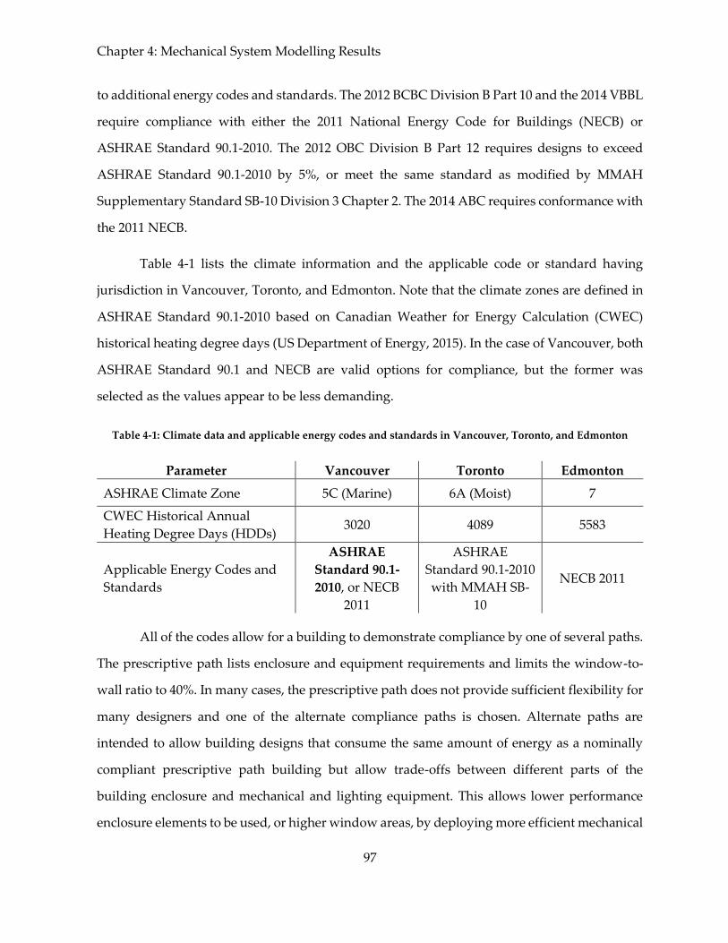
Chapter 4: Mechanical System Modelling Results
97
to additional energy codes and standards. The 2012 BCBC Division B Part 10 and the 2014 VBBL
require compliance with either the 2011 National Energy Code for Buildings (NECB) or
ASHRAE Standard 90.1-2010. The 2012 OBC Division B Part 12 requires designs to exceed
ASHRAE Standard 90.1-2010 by 5%, or meet the same standard as modified by MMAH
Supplementary Standard SB-10 Division 3 Chapter 2. The 2014 ABC requires conformance with
the 2011 NECB.
Table 4-1 lists the climate information and the applicable code or standard having
jurisdiction in Vancouver, Toronto, and Edmonton. Note that the climate zones are defined in
ASHRAE Standard 90.1-2010 based on Canadian Weather for Energy Calculation (CWEC)
historical heating degree days (US Department of Energy, 2015). In the case of Vancouver, both
ASHRAE Standard 90.1 and NECB are valid options for compliance, but the former was
selected as the values appear to be less demanding.
Table 4-1: Climate data and applicable energy codes and standards in Vancouver, Toronto, and Edmonton
Parameter Vancouver Toronto Edmonton
ASHRAE Climate Zone 5C (Marine) 6A (Moist) 7
CWEC Historical Annual
Heating Degree Days (HDDs) 3020 4089 5583
Applicable Energy Codes and
Standards
ASHRAE
Standard 90.1-
2010, or NECB
2011
ASHRAE
Standard 90.1-2010
with MMAH SB-
10
NECB 2011
All of the codes allow for a building to demonstrate compliance by one of several paths.
The prescriptive path lists enclosure and equipment requirements and limits the window-to-
wall ratio to 40%. In many cases, the prescriptive path does not provide sufficient flexibility for
many designers and one of the alternate compliance paths is chosen. Alternate paths are
intended to allow building designs that consume the same amount of energy as a nominally
compliant prescriptive path building but allow trade-offs between different parts of the
building enclosure and mechanical and lighting equipment. This allows lower performance
enclosure elements to be used, or higher window areas, by deploying more efficient mechanical

Chapter 4: Mechanical System Modelling Results
98
systems, better controls, etc. The trade-off analysis is generally conducted using an hourly
energy simulation.
Table 4-2 and Table 4-3 list the prescriptive path building enclosure overall heat transfer
coefficient and assembly insulation levels respectively based on code requirements for the three
cities in question. Note that the overall heat transfer coefficient is commonly referred to as the
U-value in imperial units, or the USI-value in metric units. Similarly, the assembly insulation
level is often discussed in terms of the R-value in imperial units, and the RSI-value in metric
units, with these values being equal to the inverse of the overall heat transfer coefficients.
Additionally, a conductance or C-value has equivalent units to a U-value.
Table 4-2: Opaque assembly overall heat transfer coefficients for Vancouver, Toronto, and Edmonton based on
prescriptive path code compliance in W/m2∙K (BTU/hr∙ft2∙°F)
Parameter Vancouver Toronto Edmonton
Maximum Above Grade Wall
U-value
USI-0.45 (U-0.08)
For mass walls
USI-0.34 (U-0.06)
For mass walls
USI-0.21
(U-0.037)
Maximum Below Grade Wall
U-value
CSI-0.67
(C-0.119)
CSI-0.52
(C-0.092)
CSI-0.284
(C-0.05)
Maximum Roof U-value
USI-0.27
(U-0.048)
For insulation
above deck
USI-0.18
(U-0.032)
For insulation
above deck
USI-0.162
(U-0.029)
Maximum Floor U-value
USI-0.36
(U-0.064)
For mass floors
USI-0.29
(U-0.051)
For mass floors
USI-0.162
(U-0.029)
Table 4-3: Opaque assembly insulation requirements for Vancouver, Toronto, and Edmonton based on
prescriptive path code compliance in m2∙K/W (hr∙ft2∙℉/BTU)
Parameter Vancouver Toronto Edmonton
Minimum Above Grade Wall
R-value
RSI-2.2 (R-12.5)
For mass walls
RSI-2.9 (R-16.7)
For mass walls
RSI-4.8
(R-27)
Minimum Below Grade Wall R-
value
RSI-1.5
(R-8.4)
RSI-1.9
(R-10.9)
RSI-3.5
(R-20)

Chapter 4: Mechanical System Modelling Results
99
Parameter Vancouver Toronto Edmonton
Minimum Roof R-value
RSI-3.7
(R-20.8)
For insulation
above deck
RSI-5.6
(R-31.2)
For insulation
above deck
RSI-6.2
(R-34.5)
Minimum Floor R-value
RSI-2.8
(R-15.6)
For mass floors
RSI-3.4
(R-19.6)
For mass floors
RSI-6.2
(R-34.5)
Table 4-4 displays the performance requirements for fenestrations in the three locations
in question based on code requirements. Note that the value of NR for the Edmonton SHGC
means that there is no code requirement.
Table 4-4: Prescriptive path code fenestration performance requirements for Vancouver, Toronto, and
Edmonton
Fenestration Parameter Vancouver Toronto Edmonton
Maximum U-value
USI-2.55
(U-0.45)
For metal framing
(curtainwall)
USI-1.99
(U-0.35)
For metal framing
(curtainwall)
USI-2.2
(U-0.39)
Maximum SHGC 0.4 0.4 NR
NECB 2011 and ASHRAE 90.1-2010 require designers to account for thermal bridging,
but only with respect to certain aspects of the building enclosure. NECB requires one to account
for closely spaced repetitive structural members such as studs, but does not require any
accommodation for thermal bridging of floor slabs, columns, or spandrels. ASHRAE 90.1
accounts for thermal bridging by providing assembly effective maximum heat transfer
coefficients while also providing the minimal nominal insulation levels. Additionally, ASHRAE
90.1 distinguishes between different types of construction within each assembly such as mass
and steel framed walls, whereas NECB simply provides a single value for each type of
assembly. All of these factors tend to result in ASHRAE maximum heat transfer values falling
higher than NECB values as stated, but the effective insulation levels would likely be equivalent
in practice. The Ontario Building Code does require floor slab projections and balconies to be
considered if they exceed 2% of the enclosure area.

Chapter 4: Mechanical System Modelling Results
100
One key requirement, not stated in Table 4-4, is that the window to wall ratio (WWR) or
fenestration and door area to gross wall area (FDWR) is limited in the prescriptive path.
ASHRAE-90.1-2010 requires a maximum WWR of 40% for all buildings, which in this context
applies to Toronto and Vancouver. NECB 2011 applies equation 4-1 to determine this ratio,
which results in a maximum FDWR of 29% in Edmonton assuming an annual average of 5583
HDDs (National Research Council Canada, 2011).
Eq. 4-1
∙
Both NECB 2011 and ASHRAE 90.1-2010 allow a trade-off procedure to supplement the
prescriptive method of meeting the energy requirements. The intent is to allow designers to
vary from the limiting requirements for different aspects of the building enclosure as long as
the building enclosure energy performance is at least equal to that of a code based building.
The most common application of this procedure in Toronto and Vancouver is to increase the
WWR far above the 40% maximum by improving the enclosure, mechanical, or lighting system
performance such that energy consumption is unaffected. NECB allows for both a simple trade-
off procedure involving a UA product balance across above grade assemblies, as well as a
detailed procedure involving energy modelling. ASHRAE Standard 90.1 however only allows
verification through energy modelling. In the context of this project, increasing the WWR is
necessary to make the buildings more representative of typical construction. In order to do this,
however, the trade-off procedures must be followed for the applicable code.
For Vancouver and Toronto, ASHRAE Standard 90.1-2010 Appendix C describes the
steps associated with the trade-off path. There are specific modeling assumptions required, but
the general methodology is that the proposed building enclosure can fail to meet one or more
of the stated requirements as long as the HVAC and lighting energy consumption in exterior
spaces and surfaces is less than or equal to a similar building which does meet all requirements.
Both buildings must have the same assumptions other than the building enclosure, and must

Chapter 4: Mechanical System Modelling Results
101
also use specific prescribed HVAC systems, setpoints, Lighting Power Densities (LPDs) and
Miscellaneous Electrical Loads (MELs). Table 4-5 displays the code-based reference model
enclosure properties for Vancouver and Toronto as determined through this path.
For Edmonton, the NECB 2011 simple trade-off path can be followed to adjust the
enclosure to meet code while providing more than the minimum WWR of 29%. Equation 4-2
was applied based on the requirements discussed in Table 4-2 through Table 4-4, and the
prescriptive path code-based reference model enclosure inputs for Edmonton can be seen in
Table 4-5 (National Research Council Canada, 2011).
Eq. 4-2
where:
∙
∙
Table 4-5: Building enclosure parameters for code-based reference models in Vancouver, Toronto, and
Edmonton based on code compliance through the applicable trade-off paths
Parameter Vancouver Toronto Edmonton
Above Grade Wall R-value RSI-2.2
(R-12.5)
RSI-4.0
(R-22.7)
RSI-5.3
(R-30)
Below Grade Wall R-value RSI-1.5
(R-8.4)
RSI-1.9
(R-10.9)
RSI-3.5
(R-20)
Roof R-value RSI-3.7
(R-20.8)
RSI-5.6
(R-31.2)
RSI-6.2
(R-34.5)
Floor R-value RSI-2.8
(R-15.6)
RSI-3.4
(R-19.6)
RSI-6.2
(R-34.5)
Window Conductance USI-1.53
(U-0.27)
USI-1.42
(U-0.25)
USI-1.53
(U-0.27)
Window SHGC 0.4 0.4 0.45
Window to Wall Ratio 65% 65% 45%

Chapter 4: Mechanical System Modelling Results
102
The values in Table 4-5 achieve compliance with the applicable building codes at the
time of publication, and therefore represent the minimum possible building enclosure which
can currently be constructed. Although the proposed trade-offs are technically valid, the
required opaque wall R-value (R-16.7 in Toronto) and window U-value (0.25 in Toronto) are
well beyond common practice: for example, an aluminum-framed window system capable of
65% WWR would need to be triple-glazed and high-performance to achieve U-0.25.
While some developers may choose to simply comply with the code, any project with
the intent of constructing a low-energy building would likely implement a much more robust
building enclosure. A low-energy building today is likely to approximate the code-compliant
building of the future. In order to accommodate buildings which exceed the code, two reference
models for each city are proposed: a code compliant model, and a low-energy model. Defining
the low-energy model building enclosure parameters is difficult and speculative and hence
beyond the scope of this study. To provide a well-researched set of low-energy building
enclosure properties a CMHC study evaluating ECMs for low-energy MURBs across Canada
was used (Canadian Mortgage and Housing Corporation, 2015). Table 4-6 displays the building
enclosure parameters for the low-energy reference models. These are quite aggressive targets,
currently at the limit of either technical or economic viability.
Table 4-6: Building enclosure parameters for low-energy reference models in Vancouver, Toronto, and
Edmonton (Canadian Mortgage and Housing Corporation, 2015)
Parameter Vancouver Toronto Edmonton
Above Grade Wall R-value RSI-4.5
(R-25.5)
RSI-5.4
(R-30.6)
RSI-5.4
(R-30.6)
Roof R-value RSI-5.6
(R-31.7)
RSI-7.4
(R-42)
RSI-9.1
(R-51.6)
Floor R-value RSI-4.6
(R-26)
RSI-4.6
(R-26)
RSI-4.6
(R-26)
Window Conductance USI-0.91
(U-0.16)
USI-0.68
(U-0.12)
USI-0.68
(U-0.12)
Window SHGC 0.55 0.39 0.39
Window to Wall Ratio 35% 30% 30%

Chapter 4: Mechanical System Modelling Results
103
4.1.4 Summary of Model Inputs Retained from Existing Building Model
With the modifications from the existing building model established, the remaining
inputs largely remain unaffected. This includes the suite heating and cooling setpoints, lighting
power densities, miscellaneous equipment loads, enclosure air leakage, and domestic hot water
demand.
The logic behind retaining certain input values in place of typical values from energy
standards or modelling guides is twofold: some values are not explicitly stated in code, and
some values stated in code are outdated and not necessarily applicable or representative of
modern construction. The values from the Belmont case study building – while taken from a
specific building – are reflective of real conditions, and while some values are the result of
calibrations, others are the same values stated in code or modelling guidelines. Table 4-7
displays the model inputs retained from the existing building calibration in Chapter 3.
Table 4-7: Building model inputs retained from the existing building model
Parameter Value Source
Suite MELs (W/ft2) 0.38 Calibration
Suite LPD (W/ft2) 0.20 Calibration
Suite DHW Demand (Gal/Apt/Day) 52 Calibration
Corridor MELs (W/ft2) 0.44 Calibration
Corridor LPD (W/ft2) 0.6 ASHRAE 90.1-2010
Parkade MELs (W/ft2) 0.18 Calibration
Parkade LPD (W/ft2) 0.25 ASHRAE 90.1-2010
Elevator Room MELs (W/ft2) 2 (Sachs, 2005)
Suite Heating Setpoint (°F) 72 Calibration
Suite Heating Setback (°F) None (Wilson et al., 2014)
Suite Cooling Setpoint (°F) 76 (Wilson et al., 2014)
Suite Cooling Setback (°F) None (Wilson et al., 2014)

Chapter 4: Mechanical System Modelling Results
104
Parameter Value Source
Ventilation Heating SP (°F) 64.4 Calibration
Enclosure Airtightness (ACH @ 50 Pa) 2.8 Calibration
The maximum suite LPD for multifamily buildings stated in ASHRAE 90.1-2010 is 0.6
W/ft2, but no recommended value is actually provided – an omission which may be addressed
in addendums to the standard (Scott, 2016). Furthermore, this value is a maximum and is only
achievable if low efficiency incandescent lighting is primarily used – an unlikely scenario for
modern construction. The MELs recommended for use in residential spaces by ASHRAE 90.1-
2010 is 0.25 W/ft2, but this is unrealistically low for modern buildings. As such, the suite LPDs
and MELs were retained from the calibration exercise.
The corridor and parking garage LPDs of 0.6 W/ft2 and 0.25 W/ft2 respectively were
retained from ASHRAE 90.1-2010, but the standard MELs of 0.25 W/ft2 and 0 W/ft2 respectively
were found to be too low based on the common energy use of The Belmont. As such, the
calibrated values are taken to be more useful, as this comprises a rather large percentage of the
annual energy consumption.
The domestic hot water demand for residential dwelling units is said to be 40 US
Gal/apartment/day in the ASHRAE 90.1 User’s Manual, which is more or less in line with the
demand calculated from consumption data of 53 US Gal/apartment/day. While the input could
have been changed to reflect the standard, studies have shown that the domestic hot water
demand varies far more than energy consumption between apartment buildings, and as such
identifying a typical consumption rate would be difficult if not impossible (Charbonneau, 2011).
Building enclosure air leakage is a very important input, but is very difficult to estimate
accurately given that the simulation cannot account for dynamically varying wind loads or
occupant operation of operable windows. The value of 3.5 ACH at 50 Pa was entered during
the calibration of The Belmont, which was then altered to 2.8 ACH at 50 Pa during the model
simplification process. On an ongoing basis, this equates to approximately 0.26 ACH of air
leakage simulated in the model based on the BS-EN-12831 methods used within DesignBuilder

Chapter 4: Mechanical System Modelling Results
105
(European committee for Standardization, 2003). This value is not particularly high or low, and
falls within the range used in other studies such as the CMHC study of low-energy MURBs
which assumed 0.1 ACH for a high performance enclosure and 0.4 ACH for a code-based
enclosure (Canadian Mortgage and Housing Corporation, 2015). Regardless of the value
selected, it is very difficult to ensure this input is correct, and so the emphasis is generally to
select an input with the correct order of magnitude, and accept that there will inherently be a
large margin of error associated with it.
4.1.5 Reference Model Load Profiles
The energy demands for each reference building are split between ventilation, heating,
cooling, domestic hot water, lighting, and miscellaneous electrical loads. The space
conditioning loads represent the amount of energy which must be added or removed from the
space in order to maintain the temperature setpoints. The ventilation energy consumption
consists of the energy required to move the volume of air specified in ASHRAE Standard 62.1
at a static pressure of 1” with no losses, along with the energy which must be added or removed
from the outdoor air stream in order to meet the supply air setpoints. The domestic hot water
demand similarly consists of the amount of energy required to heat the volume of water
demanded to the setpoint temperature, and the pumping energy associated with moving this
water against a frictional and heat pressure loss of 25 ft H2O. The lighting and miscellaneous
equipment demands are a function of the previously established inputs. Figure 4-4 displays the
energy demand by category for each reference building.
The energy demand for each reference model can be normalized by floor area, as
summarized in Table 4-8. Note that these are not energy usage intensities, as EUIs are a function
of system energy consumption rather than space loads. The energy consumption indicated by
these energy demand intensity values of the low-energy model is higher than actual measured
energy use of numerous low-energy MURBs: this is expected as the mechanical and lighting
systems, controls, and appliances have all been kept at code-minimum or industry practice.

Chapter 4: Mechanical System Modelling Results
106
Figure 4-4: Total annual energy demand by end-use category for code-based and low=energy reference
models in Vancouver, Toronto, and Edmonton
Table 4-8: Energy demand intensities for code-based and low-energy reference models in Vancouver, Toronto,
and Edmonton based on a standard floor area of 5260 m2
Parameter Vancouver Toronto Edmonton
Code-based Reference Models
Total Demand Intensity
(kWh/m2) 137 176 166
Heating Demand Intensity
(kWh/m2) 37 37 48
Cooling Demand Intensity
(kWh/m2) - 22 -
Low-Energy Reference Models
Total Demand Intensity
(kWh/m2) 119 148 150
Heating Demand Intensity
(kWh/m2) 19 17 33
Cooling Demand Intensity
(kWh/m2) - 14 -
0
200,000
400,000
600,000
800,000
1,000,000
1,200,000
Vancouver:
Code
Vancouver:
Low-Energy
Toronto:
Code
Toronto:
Low-Energy
Edmonton:
Code
Edmonton:
Low-Energy
To
tal
An
nu
al E
ner
gy
Dem
an
d,
kW
h
Reference Building
DHW (kWh) MELs (kWh) Lighting (kWh)
Heating (kWh) Cooling (kWh) Ventilation (kWh)

Chapter 4: Mechanical System Modelling Results
107
4.2 Test Set of Mechanical Systems
With the energy demands established for each reference building, a test set of
mechanical systems can be applied to the loads in question in order to establish annual energy
consumption at a system level. The mechanical systems in question are categorized as discussed
in Chapter 2, with approximately 50 independent systems to be considered for each location.
Note that these systems are not all the same across location as each city has varying functional
requirements.
The list of mechanical systems considered for each location, along with the specific
system parameters and assumptions can be found in Appendix E.
Note that in general, equipment performance characteristics are based on the best
commonly available equipment at the time of this analysis. This commitment to high
performance is in accordance with the overarching goal of determining the mechanical systems
best suited for use in low-energy buildings. Table 4-9 displays general equipment efficiencies
and COPs used for this analysis, while other performance related criteria such as part load
curves can be found in Appendix E for the particular system in question.
Table 4-9: Building model input efficiencies and COPs for various pieces of equipment based on the best
performance commonly available
Equipment Performance Source
Electric Resistance Heating 100% -
Condensing Natural Gas Boiler 𝜂𝑇 = 97% (Charbonneau, 2011)
Condensing Natural Gas Furnace 𝜂𝑇 = 95% (Charbonneau, 2011)
MAU Gas Heating Coil 𝐴𝐹𝑈𝐸 = 90% (Crowther, 2014)
MAU DX Cooling EER-11 (Crowther, 2014)
In-suite ASHP Heating HSPF-8.6 (Natural Resources
Canada, 2015)
In-suite Stacked WSHP Heating COP-5 (Daikin Applied, 2015;
Trane, 2015)

Chapter 4: Mechanical System Modelling Results
108
Equipment Performance Source
In-suite ASHP Cooling SEER-17 (Natural Resources
Canada, 2015)
In-suite Stacked WSHP Cooling EER-15 (Daikin Applied, 2015;
Trane, 2015)
Heat Recovery Ventilator
Sensible
Effectiveness:
0.8
(Tillack, Raffray, &
Pulsifer, 2001)
Energy Recovery Ventilator
Total
Effectiveness:
0.8
(Tillack et al., 2001)
Instantaneous Gas Hot Water Heater EF-0.98 (Natural Resources
Canada, 2012)
Gas Hot Water Heater (With Tank) EF-0.7 (Natural Resources
Canada, 2012)
Central Rotary or Reciprocating Chiller,
<100 tons 0.7 kW/ton
(Natural Resources
Canada, 2002)
4.3 Modelling Results
The results from the modelling of each mechanical system can be found below as sorted
by location and system number. Each system number corresponds to a system described in
Appendix E, along with the model inputs used in the simulation. Annual energy consumption
associated with each system is presented along with the associated greenhouse gas emissions
and operating utility costs. The GHG emission factors as utility pricing can be found in
Appendix F.
4.3.1 Vancouver
Figure 4-5 displays energy consumption, emissions, and operating cost for each of the
eleven Type 1 – thermal comfort systems modelled in Vancouver. For comparative purposes,
these are divided into systems which provide only heating and systems which provide both
heating and cooling. It is clear that large variations are visible between systems in all three plots.

Chapter 4: Mechanical System Modelling Results
109
The low carbon nature of the electrical grid results in negligible emissions even for electric
resistance based systems. The low cost of natural gas, however, results in substantially lower
operating costs for all combustion based systems as compared to electric systems, with ground
coupled VRF being the only electric system able to compete.
1 Electric resistance, convective heating
2 In-suite AHU with forced air electric furnace
3 In-suite AHU with forced air natural gas furnace
4 Radiant floor with centralized natural gas boiler
5 2-pipe FCUs with centralized natural gas boiler
6 Hydronic convectors with central natural gas boiler
9 PTAC, electric heating coil
10 PTHP, electric backup heating coil
13 Central VRF system, air source heat pump
14 Central VRF system, ground source heat pump
Figure 4-5: Annual energy consumption, greenhouse gas emissions, and operating costs of thermal comfort
systems in Vancouver by system number
Figure 4-6 displays energy consumption, emissions, and operating cost for each of the
eleven Type 2 – indoor air quality systems modelled in Vancouver. Systems are divided based
0 100,000 200,000 300,000
14
13
10
9
6
5
4
3
2
1
Annual Energy
Consumption, kWh
Code
Low-energy
0 20,000 40,000 60,000
Annual GHG Emissions,
kg eCO₂
Code
Low-energy
0 10,000 20,000 30,000
Annual Operating Cost,
CAD
Code
Low-energy
He
ati
ng
On
lyH
ea
tin
g &
Co
olin
g
Sy
stem
Nu
mb
er

Chapter 4: Mechanical System Modelling Results
110
on zones served, with suite only, corridor only, and suite and corridor configurations. Note that
for systems employing heat recovery, it is assumed that the additional heating load imposed
directly or indirectly on the heating system is addressed via electric resistance heating. This is
not always, or even often, the case in practice as natural gas may be used to heat the air that is
delivered by an HRV. In comparison to a traditional pressurized corridor system, all centralized
and floor based heat recovery options offer lower emissions and substantially less energy use.
However, the higher cost of electricity results in higher operating costs for these systems despite
their energy savings.
Figure 4-7 displays energy consumption, emissions, and operating cost for each of the
ten Type 3 – domestic hot water systems modelled in Vancouver. These systems are divided
into in-suite, floor based, and centralized based on the location of the energy production
components. Note that only the solar assisted DHW systems are involve loads which are
location dependent. It is evident that all electric systems boast the lowest emissions but the
highest operating costs. Solar thermal DHW with an electric backup boiler was the only electric
system which boasted operating costs in the same range as all electric resistance. Furthermore,
solar thermal systems appear to be beneficial in this case, with the solar system able to provide
a substantial portion of the annual domestic hot water heating.

Chapter 4: Mechanical System Modelling Results
111
17 In-suite Heat Recovery Ventilator (HRV)
18 In-suite Energy Recovery Ventilator (ERV)
19 Floor AHU, DOAS serving corridors, heat recovery
20 Floor AHU, DOAS serving corridors, enthalpy recovery
21 Central AHU, DOAS serving corridors, heat recovery
22 Central AHU, DOAS serving corridors, enthalpy recovery
23 Floor AHU, DOAS serving suites + corridors, heat recovery
24 Floor AHU, DOAS serving suites + corridors, enthalpy recovery
25 Central AHU, DOAS serving suites + corridors, heat recovery
26 Central AHU, DOAS serving suites + corridors, enthalpy recovery
27 Central MAU, corridor pressurization, natural gas heat
Figure 4-6: Annual energy consumption, greenhouse gas emissions, and operating costs of indoor air quality
systems in Vancouver by system number
0 75,000 150,000 225,000
27
26
25
24
23
22
21
20
19
18
17
Annual Energy
Consumption, kWh
0 500 1,000 1,500
Annual GHG Emissions,
kg eCO₂
33,600 kg
eCO₂
0 5,000 10,000 15,000Annual Operating Cost,
CAD
Su
ite
On
lyC
orr
ido
rs O
nly
Su
ite
s +
Co
rrid
ors

Chapter 4: Mechanical System Modelling Results
112
28 In-suite electric storage tank water heater
29 In-suite natural gas storage tank water heater
30 In-suite electric tankless water heater
31 In-suite natural gas tankless water heater
32 Floor electric storage tank water heater
33 Floor natural gas storage tank water heater
34 Central electric boiler with storage tanks
35 Central natural gas boiler with storage tanks
36 Central solar thermal hot water system, electric boiler
37 Central solar thermal hot water system, natural gas boiler
Figure 4-7: Annual energy consumption, greenhouse gas emissions, and operating costs of domestic hot
water systems in Vancouver by system number
Figure 4-8 displays energy consumption, emissions, and operating cost for each of the
seven combination thermal comfort and indoor air quality systems modelled in Vancouver.
These are divided into in-suite AHUs and wall-mounted terminal units which incorporate
outdoor air into the supply air stream. In-suite AHUs provided consistent delivery of outdoor
air, but all terminal unit systems struggled to consistently meet airflow requirements due to the
fact that the fan only runs when the thermostat calls for conditioning.
0 75,000 150,000 225,000
37
36
35
34
33
32
31
30
29
28
Annual Energy
Consumption, kWh
0 10,000 20,000 30,000
Annual GHG Emissions,
kg eCO₂
0 5,000 10,000 15,000
Annual Operating Cost,
CAD
In-s
uit
eF
loo
rC
en
tra
lize
dSy
stem
Nu
mb
er

Chapter 4: Mechanical System Modelling Results
113
38 In-suite AHU w/ OA heat recovery, electric furnace
39 In-suite AHU w/ OA heat recovery, natural gas furnace
40 In-suite AHU w/ OA enthalpy recovery, electric furnace
41 In-suite AHU w/ OA enthalpy recovery, natural gas furnace
42 2-pipe FCUs w/ OA intake, centralized natural gas boiler
43 PTAC, electric heating coil, OA intake, point exhaust
44 PTHP, OA intake, point exhaust
Figure 4-8: Annual energy consumption, greenhouse gas emissions, and operating costs of combination
thermal comfort and indoor air quality systems in Vancouver by system number
Figure 4-9 displays energy consumption, emissions, and operating cost for each of the
eight combination thermal comfort and domestic hot water systems modelled in Vancouver.
Systems are divided into in-suite and centralized, but all use natural gas as the energy source.
As a result, there is not a substantial variation between many of the systems in terms of energy
consumption, emissions, or operating cost. However, it can generally be observed that of the
in-suite systems, hydronic fan coils with coupled with tankless water heaters provide the lowest
energy consumption, with all centralized systems performing similarly.
0 150,000 300,000 450,000
44
43
42
41
40
39
38
Annual Energy
Consumption, kWh
Code
Low-energy
0 20,000 40,000 60,000
Annual GHG Emissions,
kg eCO₂
Code
Low-energy
0 15,000 30,000 45,000Annual Operating Cost,
CAD
Code
Low-energy
In-s
uit
e A
HU
sT
erm
ina
l
Un
its
Sy
stem
Nu
mb
er

Chapter 4: Mechanical System Modelling Results
114
52 Radiant floor, in-suite gas tank water heater
53 Hydronic convectors, in-suite gas tank water heater
54 In-suite AHU w/ HW coil, in-suite gas tank water heater
55 In-suite AHU w/ HW coil, in-suite gas tankless water heater
56 Radiant floor, central gas boiler, providing DHW
57 2-pipe FCUs, central gas boiler, providing DHW
58 In-suite AHU w/ HW coil, central gas boiler, providing DHW
59 Hydronic convectors, central gas boiler, providing DHW
Figure 4-9: Annual energy consumption, greenhouse gas emissions, and operating costs of combination
thermal comfort and domestic hot water systems in Vancouver by system number
4.3.2 Toronto
Figure 4-10 displays energy consumption, emissions, and operating cost for each of the
thirteen Type 1 – thermal comfort systems modelled in Toronto. Systems are divided into
heating only, cooling only, and heating and cooling based on the functions provided.
0 200,000 400,000 600,000
59
58
57
56
55
54
53
52
Annual Energy
Consumption, kWh
Code
Low-
energy
0 40,000 80,000 120,000
Annual GHG Emissions,
kg eCO₂
Code
Low-
energy
0 5,000 10,000 15,000 20,000
Annual Operating Cost,
CAD
Code
Low-
energy
In-s
uit
eC
en
tra
lize
d
Sy
stem
Nu
mb
er

Chapter 4: Mechanical System Modelling Results
115
1 Electric resistance, convective heating
4 Radiant floor with centralized natural gas boiler
6 Hydronic convectors/radiators with central natural gas boiler
7 PTAC, no heating
8 Chilled ceilings with central chiller, cooling tower
9 PTAC, electric heating coil
10 PTHP, electric backup heating coil
11 In-suite AHU, electric furnace, dx cooling
12 In-suite AHU, natural gas furnace, dx cooling
13 Central VRF system, air source heat pump
14 Central VRF system, ground source heat pump
15 4-pipe FCUs, central natural gas boiler, chiller, cooling tower
16 In-suite WSHP, central natural gas boiler, cooling tower
Figure 4-10: Annual energy consumption, greenhouse gas emissions, and operating costs of thermal comfort
systems in Toronto by system number
Figure 4-11 displays energy consumption, emissions, and operating cost for each of the
eleven Type 2 – ventilation systems modelled in Toronto. The amount of heating required to
0 100,000 200,000 300,000
16
15
14
13
12
11
10
9
8
7
6
4
1
Annual Energy
Consumption, kWh
Code
Low-energy
0 20,000 40,000 60,000
Annual GHG Emissions,
kg eCO₂
CodeLow-energy
0 10,000 20,000 30,000
Annual Operating Cost,
CAD
Code
Low-energy
He
ati
ng
On
ly
Co
olin
g
On
lyH
ea
tin
g &
Co
olin
g
Sy
stem
Nu
mb
er

Chapter 4: Mechanical System Modelling Results
116
meet supply setpoints results in significantly more energy consumption by pressurized
corridor systems due to the lack of heat recovery. Despite the lower cost of natural gas used in
these systems, the operating costs and GHG emissions are still higher than all systems
employing some type of heat recovery.
17 In-suite Heat Recovery Ventilator (HRV)
18 In-suite Energy Recovery Ventilator (ERV)
19 Floor AHU, DOAS serving corridors, heat recovery
20 Floor AHU, DOAS serving corridors, enthalpy recovery
21 Central AHU, DOAS serving corridors, heat recovery
22 Central AHU, DOAS serving corridors, enthalpy recovery
23 Floor AHU, DOAS serving suites + corridors, heat recovery
24 Floor AHU, DOAS serving suites + corridors, enthalpy recovery
25 Central AHU, DOAS serving suites + corridors, heat recovery
26 Central AHU, DOAS serving suites + corridors, enthalpy recovery
27 Central MAU, corridor pressurization, natural gas heat
Figure 4-11: Annual energy consumption, greenhouse gas emissions, and operating costs of indoor air quality
systems in Toronto by system number
Figure 4-12 displays energy consumption, emissions, and operating cost for each of the
ten Type 3 – domestic hot water systems modelled in Toronto. Solar thermal systems offer
0 75,000 150,000 225,000
27
26
25
24
23
22
21
20
19
18
17
Annual Energy
Consumption, kWh
330,000
kWh
0 5,000 10,000 15,000 20,000
Annual GHG Emissions,
kg eCO₂
58,200
kg
eCO₂
0 20,000 40,000 60,000
Annual Operating Cost,
CAD
Su
ite
On
lyC
orr
ido
rs O
nly
Su
ite
s +
Co
rrid
ors
Sy
stem
Nu
mb
er

Chapter 4: Mechanical System Modelling Results
117
reduced energy savings in the Toronto climate, and generally electric systems cost significantly
more to operate but produce fewer emissions.
28 In-suite electric storage tank water heater
29 In-suite natural gas storage tank water heater
30 In-suite electric tankless water heater
31 In-suite natural gas tankless water heater
32 Floor electric storage tank water heater
33 Floor natural gas storage tank water heater
34 Central electric boiler with storage tanks
35 Central natural gas boiler with storage tanks
36 Central solar thermal hot water system, electric boiler
37 Central solar thermal hot water system, natural gas boiler
Figure 4-12: Annual energy consumption, greenhouse gas emissions, and operating costs of domestic hot
water systems in Toronto by system number
Figure 4-13 displays energy consumption, emissions, and operating cost for each of the
nine combination thermal comfort and indoor air quality systems modelled in Toronto. Only
the in-suite AHUs consistently met ventilation rate requirements, and all such systems did so
using approximately the same amount of annual energy.
0 75,000 150,000 225,000
37
36
35
34
33
32
31
30
29
28
Annual Energy
Consumption, kWh
0 10,000 20,000 30,000
Annual GHG Emissions,
kg eCO₂
0 5,000 10,000 15,000
Annual Operating Cost,
CAD
In-s
uit
eF
loo
rC
en
tra
lize
dSy
stem
Nu
mb
er

Chapter 4: Mechanical System Modelling Results
118
49 4-pipe FCUs w/ OA intake, central natural gas boiler, chiller, cooling tower
43 PTAC, electric heating coil, OA intake, point exhaust
44 PTHP, OA intake, point exhaust
45 In-suite AHU w/ OA heat recovery, electric furnace, dx cooling
46 In-suite AHU w/ OA heat recovery, natural gas furnace, dx cooling
47 In-suite AHU w/ OA enthalpy recovery, electric furnace, dx cooling
48 In-suite AHU w/ OA enthalpy recovery, natural gas furnace, dx cooling
50 In-suite WSHP w/ OA heat recovery, central natural gas boiler, cooling tower
51 In-suite WSHP w/OA enthalpy recovery, central natural gas boiler, cooling tower
Figure 4-13: Annual energy consumption, greenhouse gas emissions, and operating costs of combination
thermal comfort and indoor air quality systems in Toronto by system number
Figure 4-14 displays energy consumption, emissions, and operating cost for each of the
four combination thermal comfort and domestic hot water systems modelled in Toronto. As
these systems primarily use natural gas, and Toronto functionally requires cooling, only a
limited selection of systems were considered.
0 200,000 400,000 600,000
51
50
48
47
46
45
44
43
49
Annual Energy
Consumption, kWh
Code
Low-
energy
0 20,000 40,000 60,000 80,000
Annual GHG Emissions,
kg eCO₂
Code
Low-
energy
0 20,000 40,000 60,000
Annual Operating Cost,
CAD
Code
Low-
energy
Te
rmin
al U
nit
sIn
-su
ite
AH
Us
Sy
stem
Nu
mb
er

Chapter 4: Mechanical System Modelling Results
119
60 In-suite Ducted FCU, dx cooling, in-suite natural gas storage tank water heater
61 In-suite Ducted FCU, dx cooling, in-suite natural gas tankless water heater
62 4-pipe FCUs, central natural gas boiler with storage tanks, chiller, cooling tower,
providing DHW and space conditioning
63 In-suite WSHP, central natural gas boiler with storage tanks, cooling tower,
providing DHW and space conditioning
Figure 4-14: Annual energy consumption, greenhouse gas emissions, and operating costs of combination
thermal comfort and domestic hot water systems in Toronto by system number
4.3.3 Edmonton
Figure 4-15 displays energy consumption, emissions, and operating cost for each of the
ten Type 1 – thermal comfort systems modelled in Edmonton. Due to the high carbon emissions
associated with grid electricity, systems which burn natural gas on site offer the lowest GHG
emissions. Ground coupled VRF is the only electric system which provides comparable
emissions. Furthermore, while electricity is not particularly expensive, natural gas is very
cheap, making even ground coupled VRF substantially more expensive to operate than natural
gas systems.
0 200,000 400,000 600,000
63
62
61
60
Annual Energy
Consumption, kWh
Code
Low-
energy
0 40,000 80,000 120,000
Annual GHG Emissions,
kg eCO₂
Code
Low-
energy
0 10,000 20,000 30,000
Annual Operating Cost,
CAD
Code
Low-
energy
In-s
uit
eC
en
tra
lize
d
Sy
stem
Nu
mb
er

Chapter 4: Mechanical System Modelling Results
120
1 Electric resistance, convective heating
2 In-suite AHU with forced air electric furnace
3 In-suite AHU with forced air natural gas furnace
4 Radiant floor with centralized natural gas boiler
5 2-pipe FCUs with centralized natural gas boiler
6 Hydronic convectors with central natural gas boiler
9 PTAC, electric heating coil
10 PTHP, electric backup heating coil
13 Central VRF system, air source heat pump
14 Central VRF system, ground source heat pump
Figure 4-15: Annual energy consumption, greenhouse gas emissions, and operating costs of thermal comfort
systems in Edmonton by system number
Figure 4-16 displays energy consumption, emissions, and operating cost for each of the
ten Type 2 – indoor air quality systems modelled in Edmonton. Note that pressurized corridor
systems were not simulated as both NECB 2011 and ASHRAE Standard 90.1-2010 require heat
recovery of ventilation air in climate zone 7 and higher.
0 100,000 200,000 300,000
14
13
10
9
6
5
4
3
2
1
Annual Energy
Consumption, kWh
Code
Low-energy
0 100,000 200,000 300,000
Annual GHG Emissions,
kg eCO₂
Code
Low-energy
0 10,000 20,000 30,000
Annual Operating Cost,
CAD
Code
Low-energy
He
ati
ng
On
lyH
ea
tin
g &
Co
olin
g
Sy
stem
Nu
mb
er

Chapter 4: Mechanical System Modelling Results
121
17 In-suite Heat Recovery Ventilator (HRV)
18 In-suite Energy Recovery Ventilator (ERV)
19 Floor AHU, DOAS serving corridors, heat recovery
20 Floor AHU, DOAS serving corridors, enthalpy recovery
21 Central AHU, DOAS serving corridors, heat recovery
22 Central AHU, DOAS serving corridors, enthalpy recovery
23 Floor AHU, DOAS serving suites + corridors, heat recovery
24 Floor AHU, DOAS serving suites + corridors, enthalpy recovery
25 Central AHU, DOAS serving suites + corridors, heat recovery
26 Central AHU, DOAS serving suites + corridors, enthalpy recovery
Figure 4-16: Annual energy consumption, greenhouse gas emissions, and operating costs of indoor air quality
systems in Edmonton by system number
Figure 4-17 displays energy consumption, emissions, and operating cost for each of the
ten Type 3 – domestic hot water systems modelled in Edmonton. The solar thermal systems are
the only systems involving location dependent loads, and show minimal savings over other
centralized systems.
0 75,000 150,000 225,000
26
25
24
23
22
21
20
19
18
17
Annual Energy Consumption,
kWh
0 50,000 100,000 150,000
Annual GHG Emissions,
kg eCO₂
0 10,000 20,000 30,000
Annual Operating Cost,
CAD
Su
ite
On
lyC
orr
ido
rs O
nly
Su
ite
s +
Co
rrid
orsS
yst
em N
um
ber

Chapter 4: Mechanical System Modelling Results
122
28 In-suite electric storage tank water heater
29 In-suite natural gas storage tank water heater
30 In-suite electric tankless water heater
31 In-suite natural gas tankless water heater
32 Floor electric storage tank water heater
33 Floor natural gas storage tank water heater
34 Central electric boiler with storage tanks
35 Central natural gas boiler with storage tanks
36 Central solar thermal hot water system, electric boiler
37 Central solar thermal hot water system, natural gas boiler
Figure 4-17: Annual energy consumption, greenhouse gas emissions, and operating costs of domestic hot
water systems in Edmonton by system number
Figure 4-18 displays energy consumption, emissions, and operating cost for each of the
seven combination thermal comfort and indoor air quality systems modelled in Edmonton. The
in-suite AHU’s were the only systems to consistently deliver the required ventilation rate, and
of these natural gas furnaces offer the lowest emissions and operating costs.
0 75,000 150,000 225,000
37
36
35
34
33
32
31
30
29
28
Annual Energy
Consumption, kWh
0 40,000 80,000 120,000
Annual GHG Emissions,
kg eCO₂
0 5,000 10,000 15,000
Annual Operating Cost,
CAD
In-s
uit
eF
loo
rC
en
tra
lize
d
Sy
stem
Nu
mb
er

Chapter 4: Mechanical System Modelling Results
123
38 In-suite AHU w/ OA heat recovery, electric furnace
39 In-suite AHU w/ OA heat recovery, natural gas furnace
40 In-suite AHU w/ OA enthalpy recovery, electric furnace
41 In-suite AHU w/ OA enthalpy recovery, natural gas furnace
42 2-pipe FCUs w/ OA intake, centralized natural gas boiler
43 PTAC, electric heating coil, OA intake, point exhaust
44 PTHP, OA intake, point exhaust
Figure 4-18: Annual energy consumption, greenhouse gas emissions, and operating costs of combination
thermal comfort and indoor air quality systems in Edmonton by system number
Figure 4-19 displays energy consumption, emissions, and operating cost for each of the
eight combination thermal comfort and domestic hot water systems modelled in Edmonton. As
all of these systems use natural gas, all boast similar consumption, emissions, and cost. The
annual operating cost of these systems is a small fraction as compared to the electric heating
systems presented in Figure 4-15 while also providing domestic hot water.
0 200,000 400,000 600,000
44
43
42
41
40
39
38
Annual Energy
Consumption, kWh
Code Low-energy
0 150,000 300,000 450,000
Annual GHG Emissions,
kg eCO₂
Code Low-energy
0 20,000 40,000 60,000
Annual Operating Cost,
CAD
Code Low-energy
In-s
uit
e A
HU
sT
erm
ina
l Un
its
Sy
stem
Nu
mb
er

Chapter 4: Mechanical System Modelling Results
124
52 Radiant floor, in-suite gas tank water heater
53 Hydronic convectors, in-suite gas tank water heater
54 In-suite AHU w/ HW coil, in-suite gas tank water heater
55 In-suite AHU w/ HW coil, in-suite gas tankless water heater
56 Radiant floor, central gas boiler, providing DHW
57 2-pipe FCUs, central gas boiler, providing DHW
58 In-suite AHU w/ HW coil, central gas boiler, providing DHW
59 Hydronic convectors, central gas boiler, providing DHW
Figure 4-19: Annual energy consumption, greenhouse gas emissions, and operating costs of combination
thermal comfort and domestic hot water systems in Edmonton by system number
4.4 Discussion of Modelling Assumptions
The modelling conducted was based on specific assumptions developed throughout
Chapter 3, Section 4.1 of Chapter 4, and Appendix E. While these assumptions have been
previously discussed, several aspects of the simulations conducted should be addressed as they
could influence the results.
Condensing and non-condensing boilers are configured in DesignBuilder with a multi-
variable part load performance curve which is a function of part load factor and water
temperature – either entering or leaving the boiler. The condensing curve, however, is not
comprehensive enough to distinguish between periods of non-condensing operation. For
0 200,000 400,000 600,000
59
58
57
56
55
54
53
52
Annual Energy
Consumption, kWh
Code
Low-
energy
0 40,000 80,000 120,000
Annual GHG Emissions,
kg eCO₂
Code
Low-
energy
0 5,000 10,000 15,000
Annual Operating Cost,
CAD
Code
Low-
energy
In-s
uit
eC
en
tra
lize
d
Sy
stem
Nu
mb
er

Chapter 4: Mechanical System Modelling Results
125
example, an entering water temperature of 85°C at a part-load ratio of 0.5 would still yield a
part-load factor of 1.05, which when combined with a nominal efficiency of 90% results in a
thermal efficiency of 95% for that time step. As such, it is necessary to assume when configuring
the model inputs whether or not the design boiler entering water temperature will typically be
below 55°C. This is easily achieved with radiant floor systems, but more difficult to ascertain
with FCUs as performance may vary from condensing to non-condensing depending on
equipment sizing and loop design. To be conservative, a non-condensing part load curve was
assumed for the convector based hydronic systems. Good design would strive to ensure that
the return temperature from a convector would always result in condensing.
Radiant panel systems are different from all other heating and cooling systems as more
than half of the heat transfer is in the form of radiation as opposed to convective heating of the
air. Because of this, simulating system performance based on maintaining an air temperature
setpoint yielded unrealistically high energy consumption. In order to address this, the operative
setpoint was used for radiant panel systems. In order to achieve comparable results to the other
systems, the operative temperature achieved by those systems was taken as the input. In other
words, if a convective heating system with a setpoint of 72°C would typically achieve an
operative temperature of 70.5°C, radiant systems would instead be simulated to maintain this
operative temperature directly, irrespective of air temperature.
In-suite AHUs required a slight workaround based on the systems and equipment
readily available within DesignBuilder. Packaged air handling units are easily configured, but
DesignBuilder assumes that outdoor air is included in the sizing of these systems, and setting
outdoor airflows to zero results in errors or inaccurate results. In order to address this, in-suite
PTACs were configured to perform the functions of conventional in-suite electric and natural
gas furnaces with direct expansion cooling. Fan assumptions were modified to respect the
presence of supply ductwork and/or heat exchange cores.
VRF systems cannot be modelled directly in EnergyPlus. DesignBuilder includes the
functionality necessary to perform these simulations, but the level of complexity associated
with these systems prohibits a general case approach. Instead, manufacturer data for a specific

Chapter 4: Mechanical System Modelling Results
126
system must be used, as complete system configurations involve many inputs, including 26
part-load performance curves. This reliance on preconfigured system data means that results
for VRF systems have more uncertainty than other systems. For these simulations, LG ARUN/B
outdoor units were utilized.
Solar thermal systems, as with VRF systems, are very complex to configure and require
many specific inputs unique to a given collector. As such, there is a higher degree of uncertainty
surrounding the solar DHW system results as compared to other DHW systems. Viessmann
SV1/SH1 collector data was used for the simulations, with one rooftop panel for every 3 suites.
Wall mounted terminal units providing outdoor air were explored as a means of
meeting ventilation requirements, but very limited control is possible within DesignBuilder
with respect to the air volumes these units provide. This is because outdoor air is mixed into
the supply air stream, but only when the fan is running based on the thermostat. As such, all
such systems were inconsistent in their delivery of outdoor air, although they did typically
provide comparable air change rates to the suites based on monthly averages. This was
achieved in some cases by oversizing the terminal unit airflow capacity in order to ensure
adequate outdoor air delivery when on.
Zone water-to-air heat pumps can be modelled directly within DesignBuilder, but the
implementation is somewhat limited. It is only possible to connect the heat pump to a
condenser loop which can contain cooling towers, ground exchange fields, etc. As such, it is not
possible to directly connect a boiler to the condenser loop. In addition to this, while most other
terminal units can be sized by the software with multiple preset part load curves to select from,
zone water-to-air heat pumps only offer an equation fit method. This resulted in excessive fan
and cooling energy. In order to generate reasonable results, a series of partial year runs and
approximations were conducted based on simulated results from comparable systems such as
4-pipe fan-coil units.

Chapter 5: Mechanical System Discussions
127
Chapter 5 : Mechanical System Discussions
The energy consumption, greenhouse gas emissions, and operational costs of various
mechanical systems in different cities across Canada were presented in Chapter 4. With these
values established, the overall trends in the data can be discussed in order to establish the larger
implications they hold for Canadian high-rise MURBs. Discussions in this chapter are divided
into three categories: general discussions of overarching trends, the implications of specific
system level design choices on system selection, and the best systems for specific stakeholder
groups.
5.1 General Discussions
The overarching high-level trends that are visible in the simulation results include the
effect of location and climate, the impact of the electrical grid characteristics (cost and carbon
emissions), and systems which demonstrate consistently strong or poor performance across all
locations.
5.1.1 Location and Climate
The main reason for considering three different Canadian cities throughout the analysis
was to quantify the effect of climate on mechanical systems. Building loads are impacted by
local weather, but the degree to which different types of systems are effected varies.
Indoor Air Quality systems providing ventilation demonstrate the largest correlation
with climate due to the fact that energy consumption of mechanical ventilation equipment is
directly influenced by the local climate through the conditioning of outdoor air. Thermal
comfort systems providing heating and cooling are also affected by climate, but to a lesser
degree. This is largely due to the fact that the space heating and cooling loads are connected
indirectly to the outdoor climate via the building enclosure, and the building enclosure code
requirements and local practices tend to reflect the local climate. In other words, energy codes
impose increasingly stringent requirements for building enclosure performance with increasing

Chapter 5: Mechanical System Discussions
128
climate zone number which reduces the impact climate has on thermal comfort system energy
consumption.
Figure 5-1 displays the annual energy consumption of in-suite HRVs – an indoor air
quality system – and electric baseboards – a thermal comfort system – across the three locations
modelled. Note that the rate of increase from climate zone 5 in Vancouver to climate zone 7 in
Edmonton is greater for HRVs than it is for electric baseboards.
Figure 5-1: Annual energy consumption of in-suite HRVs and electric baseboards for code-based reference
buildings in Vancouver (CZ5), Toronto (CZ6), and Edmonton (CZ7). Percentage increases are
denoted with respect to Vancouver.
Another way in which climate directly influences mechanical systems is with respect to
the functional requirements imposed by the climate which must be met by the mechanical
systems. Specifically, Toronto requires cooling whereas Vancouver and Edmonton do not.
While not a substantial load, this is an additional factor which shapes design choices.
Solar thermal domestic hot water system performance inherently relies on local solar
conditions, and is therefore correlated with climate. Throughout the simulations, the
assumptions surrounding the thermal collector array remained constant despite the fact that
typical practice would normally dictate an increase in collector areas for certain regions.
However, this did enable the direct comparison of the system across locations, which can be
seen in Figure 5-2. It is clear that solar thermal systems perform better in Vancouver than in
Toronto or Edmonton. This is likely due to higher system losses during the winter in the colder
27% increase
57% increase
6% increase
36% increase
0 75,000 150,000 225,000 300,000 375,000
Electric Baseboards
In-suite HRVs
Annual Energy Consumption, kWh
Vancouver
Toronto
Edmonton

Chapter 5: Mechanical System Discussions
129
climate zones, although variation in incident solar radiation across the locations can also impact
system performance.
Figure 5-2: Annual energy consumption of solar thermal domestic hot water systems with natural gas backup
boilers in Vancouver (CZ5), Toronto (CZ6), and Edmonton (CZ7). Percentage savings are denoted
with respect to a central natural gas boiler providing all of the DHW load.
5.1.2 Electrical Grid
High-rise MURBs, by virtue of their form factor, tend to have a low ratio of roof to
conditioned floor area, often meaning that the generation of sufficient on site electricity by
photovoltaics to completely offset annual electricity consumption is infeasible.
The greenhouse gas emissions derived from the consumption of electricity is tied to the
carbon intensity of the local electrical grid.
The greenhouse gas emissions associated with the operation of electrically powered
mechanical systems is more dependent on the carbon intensity of the electrical grid than any
other factor, including system efficiency. Figure 5-3 displays annual energy consumption and
greenhouse gas emissions for hydronic baseboards, electric baseboards, and ground source heat
pumps in Vancouver, Toronto, and Edmonton. It is clear that the high carbon intensity of the
electrical grid in Edmonton results in higher GHG emissions for all electric systems despite the
added efficiency of electric resistance and heat pump technology. Conversely, the electrical grid
in Vancouver has such low emission factors that even electric resistance heating generates
insignificant emissions, and heat pump technology only furthers this trend.
43% savings
24% savings
26% savings
0 25,000 50,000 75,000 100,000 125,000 150,000
Vancouver
Toronto
Edmonton
Central Natural Gas Boiler
Annual Energy Consumption, kWh

Chapter 5: Mechanical System Discussions
130
Figure 5-3: Annual energy consumption and greenhouse gas emissions for hydronic baseboards, electric
baseboards, and ground source heat pumps in code-based reference buildings in Vancouver
(CZ5), Toronto (CZ6), and Edmonton (CZ7)
5.1.3 Consistently Strong and Poor Performing Systems
Some specific systems demonstrated consistent performance across all locations. Heat
pump technology along with low temperature natural gas systems consistently demonstrated
low site energy consumption. Conversely, combination systems employing terminal units
supplying outdoor air consistently performed poorly in terms of site energy consumption,
along with pressurized corridor systems.
5.1.3.1 Strong Performing Systems
Heat pump technology, whether implemented in the form of PTHPs, in-suite AHUs, or
VRF systems, consistently offered the lowest site energy for thermal comfort systems. This is in
spite of the fact that heat pumps also offer cooling while many of the thermal comfort systems
considered are heating only. The merit of heat pump technology with respect to greenhouse
gas emissions and operating costs in comparison to other systems varied by location.
All hydronic natural gas thermal comfort systems employing low temperature
operation and a condensing boiler offered lower site energy consumption than high
temperature non-condensing systems or natural gas furnaces. While not quantified in the
0 100,000 200,000 300,000
Electric Baseboards
GSHP
Hydronic Baseboards
Annual Energy Consumption,
kWh
0 50,000 100,000 150,000 200,000
Annual GHG Emissions,
Kg eCO₂
Vancouver
Toronto
Edmonton

Chapter 5: Mechanical System Discussions
131
model, lower water temperatures would also reduce distribution losses. Radiant floors are
inherently low temperature systems, while fan coil units and hydronic baseboards are typically
high temperature and require special design considerations in order to function effectively at
low temperatures. For hydronic convectors this can be especially difficult, requiring increased
terminal unit heat transfer area along with low space heating loads derived either from warmer
climates, high performance enclosures, outdoor reset controls, or some combination.
Furthermore, in order to achieve low temperature operation with FCUs and convectors, higher
distribution flow rates are often required, which will increase pumping energy if piping design
is not modified. When achieved, however, all low temperature hydronic natural gas systems
offer low site energy consumption comparable to electric baseboards. In most Canadian
locations, natural gas systems offer higher emissions than electric systems in exchange for lower
operating costs, although this is not true in Alberta.
5.1.3.2 Poor Performing Systems
Among the combination thermal comfort and indoor air quality systems, many systems
fell into the category of wall-mounted terminal units providing outdoor air such as fan coil
units, PTACs, and PTHPs. All of these systems incorporate some amount of outdoor air into
the supply air stream when recirculating room air for conditioning purposes. Outdoor air can
only be provided when the fan is operating, however, which by default is only when the room
thermostat calls for conditioning. As a result, these systems tend to over ventilate during peak
periods and under ventilate during shoulder seasons. Furthermore, they impose a design trade-
off between adequate ventilation with high energy consumption or moderate energy
consumption while under ventilating the space.
Pressurized corridor ventilation systems have a long history of poor performance with
respect to delivery of outdoor air to suites, acoustics, and control of building pressures.
Modelling also demonstrated that pressurized corridors use significantly more site energy than
any other ventilation option due to the lack of heat recovery. Generally, this increased energy
consumption results in higher operational costs and GHG emissions in comparison to other

Chapter 5: Mechanical System Discussions
132
indoor air quality systems as natural gas is used in the MAU for heating. However, in
Vancouver specifically, the operating cost of the pressurized corridor system fell below that of
systems employing heat recovery due to the assumption that supplemental heating is provided
electrically in said systems. In all other cases, or if natural gas was used for supplemental
heating in Vancouver, the operational cost of a pressurized corridor system would exceed all
options employing heat recovery.
5.2 System Level Design Choices
System level design choices are early stage, high level decisions made at the beginning
of the design phase. Decisions which often dictate the selection of mechanical systems include
only providing electricity in suites, plumbing natural gas in addition to electricity to suites, and
completely separating each suite through the exclusive use of suite by suite mechanical systems.
Often these choices are made based on ownership structures or the billing policies of utilities.
However, it should be noted that modern building software and monitoring equipment enables
sub-metering of centralized system energy consumption, allowing the suite energy use to be
proportioned, provided the additional capital cost is acceptable to the owners/developers.
5.2.1 Only Electricity in Suites
Only providing electricity in suites is a common design choice given that plumbing of
natural gas to each suite can be quite expensive. This choice limits the selection of mechanical
systems to either those using electricity as the primary fuel, or centralized natural gas systems.
For electric systems, suite-by-suite solutions are often preferable as they eliminate
distribution losses while only requiring the inclusion of some extra electrical capacity as
opposed to the incremental cost of plumbing natural gas. Figure 5-4 provides a summary of
select electric thermal comfort systems for the various locations.
PTACs and PTHPs can be more expensive than an in-suite AHU with heat pump
technology if multiple units are required to serve each perimeter zone within each suite. As
such, if suite-by-suite heat pump technology is desired, it is often implemented in the form of

Chapter 5: Mechanical System Discussions
133
an in-suite AHU with either an electric furnace and direct expansion cooling or an air source
heat pump with an outdoor condensing unit mounted on the balcony, exterior wall, roof, or at
grade. The largest problem with suite-by-suite ASHPs is the placement of this outdoor unit as
locating it on the balcony takes up space, on an exterior wall detracts from aesthetics, and on
the roof or at grade is limited by vertical refrigerant piping distances in addition to significantly
increasing the refrigerant charge of each system. Due to these limitations, suite-by-suite heat
pump technology is usually only selected if cooling is required. In the absence of the need for
cooling, electric baseboards or cove heating are a lower capital cost but higher operating cost
solution.
Figure 5-4: Annual energy consumption for select electric thermal comfort systems in code-based reference
buildings in Vancouver (CZ5), Toronto (CZ6), and Edmonton (CZ7)
Central heat pump solutions such as air source or ground coupled water source VRF
systems offer the lowest site energy in exchange for higher capital costs, less industry
familiarity, and more complex sub-metering. Some of the concerns surrounding suite-by-suite
heat pump technology are alleviated by these central solutions, however, the maximum vertical
refrigerant pipe run is still an issue, requiring interstitial mechanical rooms for taller buildings.
Furthermore, the construction of a ground exchange field represents a substantial incremental
cost that is difficult to justify even in areas with high utility prices and cooling requirements.
0 75,000 150,000 225,000 300,000
Electric Baseboards
PTACs/ AHU with Electric Furnace
PTHPs/AHU with ASHP
Central VRF ASHP
Central VRF GSHP
Annual Energy Consumption, kWh
Vancouver
Toronto
Edmonton

Chapter 5: Mechanical System Discussions
134
To meet ventilation requirements, in-suite HRVs are the lowest energy electric solution,
with some form of centralized heat recovery system serving the corridors. For DHW, in-suite
electric water heaters are the lowest energy electric system.
For natural gas systems, only centralized options are possible in the absence of natural
gas distribution. All centralized systems rely on hydronic distribution, and provided low
temperature operation is achieved with a condensing gas boiler, the energy performance when
heating is comparable for all terminal unit options. Figure 5-5 displays annual energy
consumption of select centralized natural gas thermal comfort systems across the various
locations modelled.
Figure 5-5: Annual energy consumption for select centralized natural gas thermal comfort systems in code-
based reference buildings in Vancouver (CZ5), Toronto (CZ6), and Edmonton (CZ7). Note that the
FCUs and WSHPs in Toronto include cooling, while all other systems are heating only.
Radiant floors offer low maintenance, low space requirements within suites, and better
control of space operative temperatures in exchange for higher capital costs. Water source heat
pumps are another more capital cost intensive option, but offer some potential energy savings
through the ability to simultaneously heat and cool different spaces, as well as the capital cost
savings of only requiring one set of supply and return piping to each unit. Ducted fan coil units
are a cheaper option, and like WSHPs, FCUs enable the additional functions of filtration and
cooling if desired. These benefits come at the expense of more noise, and FCUs require design
as well as specification in order to achieve low temperature operation.
0 100,000 200,000 300,000
Radiant Floors
Hydronic Convectors
FCUs
WSHPs
Annual Energy Consumption, kWh
Vancouver
Toronto
Edmonton

Chapter 5: Mechanical System Discussions
135
The only centralized natural gas based indoor air quality system modelled was a
pressurized corridor system, which has high site energy consumption, GHG emissions, and
often operating costs in addition to all of the previously discussed performance issues in
exchange for low capital costs and ease of maintenance. A centralized DOAS with heat recovery
and supplemental gas heating would be a superior option from an energy and IAQ standpoint,
but would be difficult to balance in addition to having significantly higher capital costs. A more
realistic alternative to pressurized corridors would be floor by floor DOAS with heat recovery
and supplemental natural gas heating, though this would still be much more capital intensive
and require distribution of natural gas to each floor.
For natural gas DHW, a central condensing boiler with storage tanks is the cheapest and
lowest energy solution. Capital costs can potentially be lowered even further by combining the
DHW system with the thermal comfort system in order to reduce the number of boilers.
Combining suite-by-suite heat recovery ventilation with such a comfort system provides an
effective affordable system: using condensing DHW and space heating equipment would
minimize energy use.
5.2.2 Electricity and Natural Gas in Suites
The decision to pipe natural gas to each suite represents a significant incremental cost,
and is often only taken if suite-by-suite natural gas systems are desired.
The most traditional in-suite natural gas thermal comfort system is an AHU with a
natural gas furnace. These systems are easily sub-metered, less complex, and can provide
filtration and cooling via direct expansion refrigerant coils in addition to heating.
The availability of in-suite natural gas does not have a significant influence over the
choice of indoor air quality systems, although if in-suite HRVs/ERVs are to be used, combining
the supply of outdoor air into the AHU supply stream can alleviate the risk of thermal comfort
issues from poor air mixing or cold/hot ventilation air temperatures.

Chapter 5: Mechanical System Discussions
136
If DHW is also to be provided on a suite-by-suite basis, the lowest energy option is a
condensing hot water heater. While these systems are efficient, and in the case of tankless
heaters take up minimal space, they are significantly more expensive than non-condensing
storage tank hot water heaters. Combination DHW and thermal comfort systems offer potential
here, but if centralized systems are possible, a central condensing boiler providing DHW would
be a cheaper and easier to maintain option with the downside that distribution losses can
become significant.
5.2.3 Separate Suite-by-suite Systems
In some cases, whether driven by ownership structures, billing of utilities, or other
extenuating circumstances, it can be desirable to completely separate all mechanical systems by
suite. In this way, each suite contains all of the equipment necessary to provide all required
mechanical system functions.
Many suite-by-suite thermal comfort systems are available, but due to space limitations,
combination thermal comfort and DHW systems are very desirable, particularly if using natural
gas. Figure 5-6 displays a summary of all in-suite combination thermal comfort and DHW
systems modelled. Note that high efficiencies are only achieved through use of condensing
water heaters. While tankless water heaters could in theory be combined with any hydronic
system, they require more careful design than tanked systems. In addition, warmer climates
such as Toronto cannot provide a complete system with just radiant floor or hydronic convector
based systems as these cannot provide space cooling.
In the case of electric space conditioning, the best trade off of capital cost and energy
performance is provided by electric baseboards for heating only, and heat pumps with direct
expansion cooling if necessary. Note that as electric baseboard systems would not benefit from
increased efficiency through the use of combination systems, along with the fact that electric
baseboards already consume minimal suite area, a separate electric storage tank water heater
is the best choice for all-electric systems using electric baseboards.

Chapter 5: Mechanical System Discussions
137
For suite-by-suite indoor air quality systems, HRVs or ERVs, either ducted
independently or tied into the supply air stream of an in-suite AHU, provide the lowest energy
consumption. Operating costs and GHG emissions would be largely dependent on whether
natural gas or electricity was used for space heating.
Figure 5-6: Annual energy consumption for in-suite combination thermal comfort and domestic hot water
systems in code-based reference buildings in Vancouver (CZ5), Toronto (CZ6), and Edmonton
(CZ7). Note that the FCUs in Toronto include cooling, while all other systems are heating only.
5.3 Stakeholders
Stakeholders represent different parties involved in the construction and operation of
high-rise MURBs, each with different priorities. As these priorities dictate the relative ranking
of different mechanical system characteristics, each stakeholder group will have a different
viewpoint on what constitutes the best mechanical system. By considering each group
separately, one can form recommendations for a wide variety of use cases.
In-suite Ducted FCU, in-suite gas tankless water
heater
In-suite Ducted FCU, in-suite gas tank water
heater
Hydronic convectors, in-suite gas tank water
heater
Radiant floor, in-suite gas tank water heater
Electric baseboard, in-suite storage tank water
heater
0 100,000 200,000 300,000 400,000 500,000
Annual Energy Consumption, kWhVancouver Toronto Edmonton

Chapter 5: Mechanical System Discussions
138
5.3.1 Condo Owners
Condo owners are people who choose to purchase a suite in a given high-rise MURB,
thereby taking ownership over that portion of the building along with obligations to condition
and maintain the common spaces. Condo owners generally are more concerned with the long
term value of the property rather than the initial sale. Furthermore, condo owners typically
prioritize ease of maintenance, low operating costs, aesthetics, and acoustics. However, condo
owners rarely, if ever, understand, or have influence over, the myriad factors that influence the
performance of a building, or are in position to judge the often very favourable cost-benefit
trade-offs for investing slightly more to gain a much lower operating cost solution.
The choice of thermal comfort system varies depending on whether cooling is required
or not. Without a need for cooling, radiant floors with central natural gas boilers offer low
energy use, low operating costs, central access for maintenance, no noise, and no impact on
suite aesthetics other than some restrictions on floor coverings. If cooling is required, in-suite
ducted 4-pipe FCUs offer low operating costs and low in-suite maintenance requirements.
Aesthetic impact can be minimized by placing the unit in a mechanical closet and hiding ducts
in bulkheads, however the acoustic impact is dependent on the design of the air distribution
ductwork.
A floor by floor dedicated outdoor air system with ducted supply and return from each
unit would typically offer the lowest operating cost and the lowest in-suite maintenance of any
of the indoor air quality systems modelled. The impact on suite aesthetics can be minimized
through the use of bulkheads to conceal ductwork. Acoustics can be a concern as noise transfer
between units is dependent on the design of the air distribution ductwork.
A central condensing natural gas boiler providing DHW is the cheapest domestic hot
water system from an operating cost perspective if distrivution piping losses and recirculating
pumping energy are tightly managed. Furthermore, no space is required within each suite for
equipment, and maintenance is centralized. This system is commonly implemented without
any form of sub-metering, requiring communal sharing of DHW operating costs. If sub-

Chapter 5: Mechanical System Discussions
139
metering of DHW is desired, it is typically achieved via in-suite systems. The lowest operating
cost in-suite DHW system is a condensing natural gas water heater.
5.3.2 Managers of Rental Properties
Managers of rental properties either retain ownership of the entire building or act on
behalf of the building owner, and oversee daily operations and maintenance. In some cases, the
manager is also the developer behind the project. As such, maintenance costs as well as ease of
access to perform maintenance are both important system characteristics, along with
minimizing operating costs. Ease of sub-metering is not as important because utilities are often
handled directly by the property manager. Furthermore, capital costs may also be of importance
depending on the relationship between the manager and the developer.
Selecting a thermal comfort system which offers low capital costs, low operating costs,
and low maintenance is a difficult balance. Electric baseboards are often selected for their low
maintenance and low capital cost, but the price of electricity results in high operating costs in
all locations. Hydronic baseboards represent a compromise which still offers fairly low capital
cost, low maintenance, as well as low operating cost despite the fact that many systems still
operate in non-condensing mode. Note that high temperature non-condensing hydronic
systems, while notably less efficient than condensing systems, are still fairly cheap to operate
in comparison to electric systems given the low cost of natural gas. For a higher capital cost but
lower operating cost, radiant floors would offer even lower maintenance requirements as there
are no convectors to become damaged or dirty. If cooling is required, ducted 4-pipe FCUs
would offer cooling and filtration with minimal additional in-suite maintenance beyond filter
changes.
There is no clear choice for indoor air quality system beyond the inclusion of heat
recovery. It is difficult to recommend pressurized corridor systems because of their poor
ventilation performance and the complaints associated with odour and noise transmission from
corridors to suites. In-suite HRVs/ERVs would offer low operating costs, but have higher
capital costs than pressurized corridor systems and require suite access for maintenance. Floor

Chapter 5: Mechanical System Discussions
140
by floor DOAS with heat recovery would also offer low operating costs while removing the
need for suite access, but the capital costs associated with these systems can be high due to the
need for extensive supply and return ductwork, fire dampers between units, and ceiling space
within corridors.
For domestic hot water, the lowest capital and operating cost solution would a central
condensing natural gas boiler. In this case, given the need for a boiler plant as part of the
thermal comfort system anyways, some capital cost could be saved by using the same boiler
plant to also provide domestic hot water.
5.3.3 Developers of Condo Properties
Developers of condo properties fund the construction of high-rise MURBs for the
express purpose of selling condo properties for profit. As such, capital cost, constructability,
and aesthetics rank highly in terms of typical priorities. However, developers do try to cater to
a market need, and so as other system characteristics such as greenhouse gas emissions become
more important to general consumers, some developers will try to adjust their product to stay
competitive, while many continue to focus on meeting code and selling visible features.
The lowest capital cost thermal comfort system for heating only climates is electric
baseboards, with hydronic baseboards providing a slightly more expensive alternative if there
is market demand for natural gas heating. Both systems take up minimal space within units,
and are simple from a controls and constructability standpoint. If cooling is required, in-suite
AHUs with electric furnaces and direct expansion cooling represents one of the cheapest and
simplest options. If natural gas heating is desired, 2-pipe ducted FCUs with a central boiler and
chiller would have relatively low capital cost compared to other heating and cooling systems.
The lowest capital cost indoor air quality system is pressurized corridor ventilation,
although it is not permitted by building and energy codes in the coldest areas of Canada (CZ7
and CZ8). There are many well demonstrated performance issues with these systems, however,
and as the demand for better indoor air quality increases, the increased capital cost of in-suite
HRVs will likely become justified to meet market demand.
Chapter 5: Mechanical System Discussions
141
Central natural gas boilers offer the lowest capital cost domestic hot water solution,
while also being typical practice within the industry.
5.3.4 Policy Makers
Policy makers are responsible for setting targets and requirements for the building
industry through building codes and standards. Priorities of policy makers vary over time, but
current high priorities involve reducing site energy consumption, reducing greenhouse gas
emissions, and ensuring adequate indoor air quality.
Greenhouse gas emissions, as discussed in Section 5.1.2, are highly dependent on the
carbon intensity of the electrical grid from which a given building sources its power. However,
as the movement continues towards lower carbon grids in keeping with provincial and national
carbon reduction objectives, the carbon intensity of grid electricity will play less of a factor and
site energy consumption will become more important in all jurisdictions.
Within thermal comfort systems, heat pump technology provides the lowest site energy
consumption. VRF heat pumps offer some added performance over typical packaged,
distributed heat pumps given the ability to provide simultaneous heating and cooling during
shoulder seasons. This comes at the price of higher risk due to lack of familiarity within the
industry, as well as more potential for refrigerant leakage given the large charge of each system.
Furthermore, ground source heat pumps improve performance over air source heat pumps
given that heat pump COPs are a function of source temperature, and the ground temperature
never drops below freezing in most Canadian cities. While VRF systems can be marginally to
moderately more expansive than traditional FCU based hydronic systems, ground exchange
fields are very capital cost intensive to construct making payback difficult to justify.
Electric resistance heating can offer a compelling balance of low risk, low maintenance,
simple controls, and low capital cost. Provided additional resources are expended reducing
heat loss by improving HRV’s and the building enclosure, electric resistance heating systems
may become popular again across Canada. Heat pump technology would further reduce GHG

Chapter 5: Mechanical System Discussions
142
emissions, but for low carbon grids in heating only climates, the incremental reduction likely is
not warranted by the emissions reductions alone.
Within indoor air quality systems, heat recovery is the most effective means of reducing
energy consumption and GHG emissions in comparison to traditional pressurized corridor
systems. The three most common ways of implementing heat recovery are in-suite HRVs or
ERVs, in-suite AHUs providing space conditioning as well as ventilation, and floor based
dedicated outdoor air systems with ducted supply and return from each suite.
Solar thermal systems offer the lowest domestic hot water energy consumption of any
of the systems modelled, particularly if an electric backup boiler is implemented. However,
these systems are more expensive than other options, and energy savings vary by location for
the same load and solar thermal array. Furthermore, due to the form factor of high rise MURBs,
as the number of floors increases, the ratio of roof area to DHW load decreases. This results in
a decrease in savings due to insufficient solar resource. Solar thermal systems are therefore
more suited for use in low- and mid-rise MURBs.
In-suite electric storage tank water heaters offer the lowest site energy consumption
following solar thermal systems with lower capital costs and less system complexity. For low
carbon grids, these systems would also offer GHG reductions over traditional central natural
gas boilers.

Chapter 6: Conclusions and Recommendations
143
Chapter 6 : Conclusions and Recommendations
Mechanical systems currently implemented in Canadian high-rise MURBs are diverse
and numerous, each with specific characteristics driving their selection. Through the review of
literature and building simulations, conclusions can be drawn with respect to the selection of
mechanical systems, and recommendations can be formed with respect to future work.
6.1 Conclusions
Location and climate tend to impact ventilation loads significantly, while only modestly
impacting space conditioning loads as the building enclosure performance, because of building
codes and local construction practices, reflect the severity of climate in which they are situated.
The carbon intensity of the electrical grid is the largest determining factor for mechanical
system greenhouse gas emissions in applications using electricity as the primary fuel source.
Heat pump technology, however it is implemented, delivers the lowest site energy
consumption of all available technologies. Operating cost and greenhouse gas emissions are not
necessarily lower than other options, and are dependent on the climate and electrical grid.
All low temperature hydronic systems with condensing natural gas boilers deliver
comparable energy performance, regardless of terminal unit.
Air-to-air heat recovery, however it is implemented, significantly reduces ventilation
energy consumption and greenhouse gas emissions relative to pressurized corridor systems.
Operating cost savings are dependent on location and climate.
Combination thermal comfort and domestic hot water systems powered by natural gas
offer a suite-by-suite alternative to centralized natural gas systems that may require more
maintenance but offer reduced distribution losses, sub-metering of domestic water and space
heating at a small increase in site energy consumption.

Chapter 6: Conclusions and Recommendations
144
Solar thermal domestic hot water systems offer potential reduction in site energy
consumption, greenhouse gas emissions, and operating cost over traditional systems in low-
and mid-rise MURBs. In high-rise construction, the ratio of roof area to load decreases with
building height such that the savings potential drops off from lack of available solar resource.
Rational mechanical system selection should be based on the relative importance of
competing system characteristics. However, the ranking of important characteristics varies
amongst different stakeholder groups, and is partly subjective. Thus, system recommendations
for different stakeholder groups vary and no clear best practice option emerged from the
analysis.
6.2 Recommendations
While the scope of this thesis was quite broad, it could be expanded in a number of ways
to further explore this area. Low- and mid-rise MURBs could be evaluated to determine lower
building height might impact system selections. Furthermore, more reference buildings could
be added to the modelling analysis to reflect different form factors, lower enclosure to
conditioned floor area ratios, and lower suite areas.
The energy modelling analysis demonstrated little variation in energy consumption
between centralized and distributed hydronic systems due to the fact that pumps were
assumed to be perfectly sized, operating at ideal part load ratios, with no thermal distribution
losses through the pipework. These assumptions were necessary for this analysis, but field
experience suggests the relative magnitude of the distribution losses is large and poorly
quantified. A targeted study could measure the thermal output of the central plant while also
measuring the heat transferred to or from terminal units within each suite in a representative
high-rise MURB. Through these measurements, the magnitude of distribution losses could be
quantified.
Heat pump technology demonstrated the lowest site energy, and can be implemented
for space conditioning as well as domestic hot water. Few systems are available for DHW

Chapter 6: Conclusions and Recommendations
145
supply in North America. The added complexity of the system tends to make this performance
more capital cost intensive, and the use of electricity over natural gas can make operating costs
more expensive than competing traditional technologies. A targeted study could focus on the
use of heat pump technology specifically in order to identify key factors and scenarios in which
such technology can be cost competitive in high-rise MURBs.

References
146
References
Afify, R. (2008). Designing VRF systems. ASHRAE Journal, 50(6), 52–55.
American Society of Heating Refrigerating and Air-Conditioning Engineers. (2002). ASHRAE
Guideline 14-2002 Measurement of Energy and Demand Savings. Ashrae, 8400, 170.
American Society of Heating Refrigerating and Air-Conditioning Engineers. (2004). ASHRAE
Standard 90.1-2004: User’s Manual. Atlanta, GA.
American Society of Heating Refrigerating and Air-Conditioning Engineers. (2007). ASHRAE
Standard 90.1-2007: Energy Standard for Buildings Except Low-rise Residential Buildings.
Atlanta, GA.
American Society of Heating Refrigerating and Air-Conditioning Engineers. (2009). 2009
ASHRAE Handbook -Fundamentals. Atlanta, GA.
American Society of Heating Refrigerating and Air-Conditioning Engineers. (2012). 2012
ASHRAE Handbook - HVAC Systems and Equipment (2012th ed.). Atlanta, GA, GA.
American Society of Heating Refrigerating and Air-Conditioning Engineers. (2013). ASHRAE
Standard 55-2013: Thermal Environmental Conditions for Human Occupancy. Atlanta, GA.
American Society of Heating Refrigerating and Air-Conditioning Engineers. (2015). 2015
ASHRAE Handbook - HVAC Applications. (M. S. Owen, Ed.) (SI Edition). Atlanta, GA.
American Society of Heating Refrigerating and Air-Conditioning Engineers. (2016). ASHRAE
Standard 62.1-2016: Ventilation for Acceptable Indoor Air Quality. Standard, American
National Standards Institute. http://doi.org/ANSI/ASHRAE Standard 62.1-2004
Baxter, V., Fischer, S., & Sand, J. R. (1998). Global Warming Implications of Replacing Ozone-
Depleting Refregierants. ASHRAE Journal, (September), 23–30.
BC Ministry of Environment. (2014). 2014 BC Best Practices Methodology for Quantifying
Greenhouse Gas Emissions. Victoria, BC.
Bhatia, A. (2012). Design Options for HVAC Distribution Systems. Course, Stony Point, NY:
Continuing Education and Development, Inc.
Boldt, J., & Keen, J. (2015). Hydronics 101. ASHRAE Journal, 57(5), 62–70.

References
147
Borgnakke, C., & Sonntag, R. E. (2009). Fundamentals of Thermodynamics. (N. Repasky, Ed.) (7th
Editio). Danvers, MA: John Wiley & Sons, Inc.
Butcher, T. (2011). Performance of combination hydronic systems. ASHRAE Journal, 53(12),
36–41.
Canada Green Building Council. (2010). LEED ® Canada Reference Guide for Green Building
Design and Construction 2009. Ottawa, ON.
Canadian Mortgage and Housing Corporation. (2001). A Guide to Mechanical Equipment for
Healthy Indoor Environments.
Canadian Mortgage and Housing Corporation. (2002). Investigation of a Ground-Source Heat
Pump Retrofit to an Electrically Heated Multi-Family Building. Mississauga, Ontario.
Canadian Mortgage and Housing Corporation. (2003). Ventilation Systems for Multi-Unit
Residential Building: Performance Requirements and Alternative Approaches.
Canadian Mortgage and Housing Corporation. (2004). Survey of In-Suite Space and Domestic
Hot Water Heating Systems in Multi-residential Buildings. Ottawa, ON.
Canadian Mortgage and Housing Corporation. (2007). Air Leakage Control Manual Existing
Multi-Unit Residential Buildings.
Canadian Mortgage and Housing Corporation. (2012). Occupied Housing Stock by Structure
Type and Tenure, Canada, 1991-2011. Retrieved October 1, 2014, from http://www.cmhc-
schl.gc.ca/en/corp/about/cahoob/data/data_007.cfm
Canadian Mortgage and Housing Corporation. (2015). Energy Simulations of Strategies to
Achieve Low-Energy , Multi-unit Residential Building Designs in Different Regions of Canada.
Ottawa, ON.
Canadian Passive House Institute. (2016). Canadian Passive House Building Certification.
Retrieved May 13, 2016, from http://www.passivehouse.ca/building-certification
Charbonneau, M. (2011). Simulating the Effects of Enclosure Retrofits on Post-War High-Rise
Apartment Buildings in Cold Climates. University of Waterloo.
City of Vancouver. (2014). Green Buildings Policy for Rezonings. Vancouver, BC: Planning
and Development Services. Retrieved from
http://former.vancouver.ca/commsvcs/guidelines/G015.pdf
Clinton, B. (1999). Using Water Heaters for Radiant Heat. Journal of Light Construction, 1–9.

References
148
Cole, R. J., & Kernan, P. C. (1996). Life-cycle energy use in office buildings. Building and
Environment, 31(4), 307–317. http://doi.org/10.1016/0360-1323(96)00017-0
Cooperman, A., Dieckmann, J., & Brodrick, J. (2012). Commercial GSHPs. ASHRAE Journal,
54(5), 84–88.
Critchley, J. (2011). Draft Environmental Code of Practice for Elimination of Fluorocarbon Emissions
from Refrigeration and Air Conditioning Systems.
Crowther, H. (2014). Energy-Efficient Makeup Air Units. ASHRAE Journal, (March), 5.
Daikin Applied. (2015). Stacked Water Source Heat Pumps. Product Brochure. Retrieved from
http://lit.daikinapplied.com/bizlit/DocumentStorage/WaterSourceHeatPump/Brochures/
ASP_31-272_WS_VHC-VHW-VHF_V-Stack_LR.pdf
Dale, J. D., Wilson, D. J., Ackerman, M. Y., & Fleming, N. P. (2000). Design Guidelines for
Combustion Air Systems. ASHRAE Journal, (May), 1–8.
DesignBuilder Software. (2008). DesignBuilder Simulation + CFD Training Guide, 1–224.
Retrieved from http://www.designbuilder.co.uk/downloadsv1/doc/DesignBuilder-
Simulation-Training-Manual.pdf
Energy Star. (2013). Source Energy.
Energy Star. (2016). Energy Efficient New Homes - Certified Apartments and Condos.
Retrieved May 13, 2016, from
https://www.energystar.gov/newhomes/certified_apartments_and_condos
European committee for Standardization. (2003). BS EN 12831: Heating systems in buildings —
Method for calculation of the design heat load. British Standard.
Fortis BC. (2015). Heating Content Values. Retrieved November 13, 2015, from
http://www.fortisbc.com/NaturalGas/Business/PriceAndMarketInformation/Pages/Heat-
content-values.aspx
Goetzler, W. (2007). Variable Refrigerant Flow Systems. ASHRAE Journal, (April).
http://doi.org/10.1016/j.enbuild.2010.01.024
Government of Alberta. (2015). Electricity Statistics. Retrieved January 25, 2016, from
http://www.energy.alberta.ca/electricity/682.asp
Government of Canada. (2015). Canadian Climate Data. Retrieved November 13, 2015, from
http://climate.weather.gc.ca/

References
149
Hanam, B. (2010). Development of an Open Source Hourly Building Energy Modeling Software Tool.
University of Waterloo.
Handegord, G. (2001). A New Approach to Ventilation of High Rise Apartments. In The Eighth
Conference on Building Science and Technology. Toronto, Ontario: Ontario Building
Envelope Council.
Heller, J., & Cejudo, C. (2009). Reverse Cycle Chillers for Multifamily Buildings in the Pacific
Northwest : Phase I Final Report. Seattle, WA, WA.
Ihnen, J. L., Weitner, S. L., & Donnell, P. C. O. (2012). Rescuing New Construction from
Widgetitis with Simple HVAC Design. ACEEE.
Independent Electricity System Operator. (2016). Power Data - Supply Overview. Retrieved
January 25, 2016, from https://ieso-public.sharepoint.com/Pages/Power-
Data/Supply.aspx
International Code Council. (2014). 2015 International Building Code. County Club Hills, IL.
Retrieved from http://codes.iccsafe.org/app/book/toc/2015/I-Codes/2015 IBC
HTML/index.html
IPMVP Comittee. (2002). International Performance Measurement & Verification Protocol. Oak
Ridge, TN.
John, D. A. (2014). Proper Specification of Air Terminal Enits. ASHRAE Journal, 56(9), 26–35.
Kavanaugh, S. (1998). Ground Source Heat Pumps. ASHRAE Journal, 39(October), 31–36.
Kavanaugh, S. P. (2016). A Simple Approach To Affordable GSHPs. ASHRAE Journal, (April),
14–24.
Lampugnani, G., & Zgliczynski, M. (1996). R290 as a Substitute of R502 and R22 in Commercial
Refrigeration and Air Conditioning. International Compressor Engineering Conference.
Liu, R. (2007). Energy Consumption and Energy Intensity in Multi-Unit Residential Buildings
( MURBs ) in Canada, (April). http://doi.org/CBEEDAC 2007–RP-04
Lstiburek, J. (2006). Building Science Digest 110: HVAC in Multifamily Buildings.
BSC/ASHRAE, (2001).
Lutz, J., Dunham-Whitehead, C., Lekov, A., & McMahon, J. (2004). Modeling Energy
Consumption of Residential Furnaces and Boilers in U.S. Homes. Berkley, CA, CA.

References
150
Mather, D. (2014). Aspects of Interior Lighting Systems. Building Energy Performance, 1–40.
Mather, D. (2015). Notes from meeting with David Mather. Conversation, Waterloo, ON.
Maxwell, S., Berger, D., & Zuluaga, M. (2014). Evaluation of Ventilation Strategies in New
Construction Multifamily Buildings, (July).
McQuiston, F. C., Parker, J. D., & Spitler, J. D. (2005). Heating, Ventilating, and Air Conditioning
(6th ed.). Danvers, MA: John Wiley & Sons, Inc.
Nall, D. H. (2013). Thermally Active Floors - Part 1. ASHRAE Journal, 55(January), 32–46.
NASA. (2014). Global Temperature. Retrieved January 14, 2016, from
http://climate.nasa.gov/vital-signs/global-temperature/
National Research Council Canada. (2011). National Energy Code of Canada for Buildings
2011. Ottawa, ON: Natural Resources Canada.
National Research Council of Canada. (1999). Model National Energy Code for Buildings:
Performance Compliance for Buildings.
Natural Resources Canada. (2002). Choosing a High-Efficiency Chiller System. Guide, Ottawa,
ON: Office of Energy Efficiency. Retrieved from
http://www.nrcan.gc.ca/sites/www.nrcan.gc.ca/files/oee/pdf/Publications/infosource/Pub
/ici/eii/pdf/m92-242-2002-1E.pdf
Natural Resources Canada. (2012). Water Heater Guide. Ottawa, ON: Office of Energy
Efficiency.
Natural Resources Canada. (2014). Energy Use Data Handbook: 1990-2011. Retrieved from
http://oee.nrcan.gc.ca/publications/statistics/handbook2010/handbook2013.pdf
Natural Resources Canada. (2015). Air-Source Heat Pumps. Retrieved April 4, 2016, from
http://www.nrcan.gc.ca/energy/publications/efficiency/heating-heat-pump/6831
Olesen, B. W. (2002). Radiant Floor Heating - In Theory and Practice. ASHRAE Journal, 44(7),
19–26.
Pigg, S. (2003). The Electric Side of Gas Furnaces. Home Energy, (December), 24–28.
RDH Building Engineering. (2012). Energy Consumption and Conservation in Mid- and High-Rise
Residential Buildings in British Columbia. Vancouver, BC.

References
151
RDH Building Sciences. (2005). Multi-Unit Residential HVAC System Guidelines. Seattle, WA.
Ricketts, L. (2014). A Field Study of Airflow in a High-Rise Multi-Unit Residential Building.
University of Waterloo.
Roth, B. K., Westphalen, D., & Brodrick, J. (2006). Ductless Split Systems. ASHRAE Journal,
48(July).
Rudd, A. (2012). Measure Guideline : Combination Forced-Air Space and Tankless Domestic Hot
Water Heating Systems. Somerville, MA.
Sachs, H. M. (2005). Opportunities for Elevator Energy Efficiency Improvements. Washington, D.C.
Retrieved from http://pt.energytaxincentives.org/files/pdf/white-paper/elevators2005.pdf
Scott, J. (2016). Lighting Requirements For High Rise Dwellings Proposed For Energy
Standard. Retrieved April 4, 2016, from https://www.ashrae.org/news/2016/lighting-
requirements-for-high-rise-dwellings-proposed-for-energy-standard
Seattle Office of Sustainability & Environment. (2015). Building Energy Benchmarking Analysis
Report 2013 Data. Seattle, WA. Retrieved from
http://www.seattle.gov/Documents/Departments/OSE/EBR-2013-report.pdf
Straube, J. (2009). Building Science Insight 022: The Perfect HVAC, 1–5.
Straube, J. F. (2014). Indoor Environmental Control Systems : Mechanical HVAC Systems.
Waterloo.
The Viessmann Group. (2004). Condensing Technology. Shropshire, GB.
Thomsen, K. E., Wittchen, K. B., & EuroACE. (2008). European National Strategies to Move
Towards Very Low Energy Buildings. Aalborg, Denmark: Danish Building Research
Institute.
Tillack, M. S., Raffray, A. R., & Pulsifer, J. E. (2001). Improved Performance of Energy Recovery
Ventilators Using Advanced Heat Transfer Media. San Diego.
Touchie, M. F., Binkley, C., & Pressnail, K. D. (2013). Correlating energy consumption with
multi-unit residential building characteristics in the city of Toronto. Energy and Buildings,
66, 648–656. http://doi.org/10.1016/j.enbuild.2013.07.068

References
152
Trane. (2015). Trane Axiom Vertical Stack Water Source Heat Pump. Retrieved from
http://www.trane.com/content/dam/Trane/Commercial/global/products-
systems/equipment/unitary/water-source-heat-pumps/vertical-stack-wshp/WSHP-
SLB046-EN_01292015.pdf
Ueno, K. (2010a). Building Science Digest 152 Building Energy Performance Metrics.
BSC/ASHRAE.
Ueno, K. (2010b). ECM Efficiency - Better and Worse Than You Think. Home Energy, May/June,
0–3. Retrieved from homeenergy.org
Ueno, K., & Straube, J. (2010). Understanding Primary/Source and Site Energy. Building
Science Digest, 151. Retrieved from
http://www.buildingscience.com/documents/digests/bsd151-understanding-primary-
source-site-energy/files/BSD-151 Source-Site_Energy.pdf
US Department of Energy. (2015). Weather Data - North and Central America WMO Region 4:
Canada. Retrieved November 14, 2015, from
http://apps1.eere.energy.gov/buildings/energyplus/cfm/weather_data3.cfm/region=4_nor
th_and_central_america_wmo_region_4/country=3_canada/cname=CANADA
US Department of Energy. (2016). Electric Resistance Heating. Retrieved May 5, 2016, from
http://energy.gov/energysaver/electric-resistance-heating
Walsh Construction Co. (2010). Energy Use and Life Cycle Cost Analysis of Mechanical
Components for Green Affordable MURBs. Seattle, WA.
Walsh Construction Co. (2011). Energy Efficient Mechanical Systems For Green Affordable Multi-
Unit Residential Buildings. Seattle, WA.
Whiticar, M. (2012). Where Our Electricity Comes From. Retrieved January 25, 2016, from
http://www.energybc.ca/map/bcenergymap.html
Wilson, E., Engebrecht Metzger, C. ., Horowitz, S., & Hendron, R. (2014). 2014 Building
America House Simulation Protocols (NREL/TP-5500-60988), (December).
Yoo, J. H. (2015). Evaluation of Solar Hot Water Heating System Applications to High-Rise
Multi-Family Housing Complex Based on Three Years of System Operation. Energy and
Buildings, 101, 54–63. http://doi.org/10.1016/j.enbuild.2015.04.037
Zimmerman, R. (2013). Sound Advice - Acoustical Specifications for Air Terminals & Air
Outlets. ASHRAE Journal, (July 2013), 1–5. http://doi.org/10.1016/S0262-4079(15)30794-6

References
153
Zogg, R., Dieckmann, J., Roth, K., & Brodrick, J. (2005). Heat Pump Water Heaters. ASHRAE
Journal, (March), 98–99.
Appendix A: Energy Use in Buildings
154
Appendix A: Energy Use in Buildings
Energy use in buildings has been an area of increasing study over the past few decades.
Between the residential and commercial sector, buildings use 30% of secondary energy in
Canada (Natural Resources Canada, 2014). In order to discuss energy and buildings, several
key concepts must be introduced, including energy sources, energy sinks, source vs. site energy,
global warming potential, the Canadian energy grid, normalized energy metrics, and the
definition of a low-energy building.
A.1 Energy Sources
Before energy can be used in buildings, it must first be captured from an energy source.
In a broad sense, all energy on earth originally came from the sun, but the specific
intermediaries through which it is captured can vary. Typically, primary energy is sourced
through one of the following practices:
1. Fossil fuel combustion to release thermal energy
2. Biomass or biogas combustion to release thermal energy
3. Nuclear decay of radioactive materials to release thermal energy
4. Solar energy, captured either as thermal energy or as electricity via photovoltaics
5. Gravitational energy, captured from falling water (hydro), wind, or waves as
kinetic energy
6. Geothermal energy from the Earth’s core captured as thermal energy
Note that many of the above energy sources provide thermal or kinetic energy which is
difficult to transport over large distances and is of low energy quality. For this reason, the
energy derived from these sources is often converted into other forms which have more
desirable characteristics such as electricity or hydrogen. It is incorrect to refer to electricity or
hydrogen as energy sources however as they are more correctly identified as forms of energy
transmission.

Appendix A: Energy Use in Buildings
155
A.2 Energy Sinks
In contrast to energy sources, energy sinks are places to which unwanted thermal
energy is rejected – typically in space cooling applications. In the context of buildings, these
usually are limited to the following:
1. Air surrounding a building
2. Bodies of water in close proximity to a building, such as ponds, rivers, or ground
water.
3. Soil adjacent to or underneath a building
Note that in the specific case of vapour compression refrigeration technology, these
energy sinks can also serve as thermal energy sources.
A.3 Source vs. Site Energy
Converting energy to different forms, along with transporting energy over large
distances has associated losses as required by the second law of thermodynamics. Energy from
one of the sources discussed in Section A.1 is referred to as source energy, and serves as a
reference point. From there it is frequently converted to a more preferable energy transport
medium such as electricity with substantial losses. The energy is then transported from the
location of the energy source to the building, which may be as small a distance as a few meters
in the case of rooftop photovoltaic panels, or as large a distance as hundreds of kilometers in
the case of large scale power plants.
The proportion of source energy consumed per unit of energy available at a given
building site is referred to as the source-to-site ratio, and varies by location, time, and form of
energy transmission. As such, most published values only discuss conversions at a national or
provincial level as the true source-to-site ratio at a specific building is often very difficult to
calculate.

Appendix A: Energy Use in Buildings
156
While any energy source discussed in Section A.1 could be used at a building level,
typical discussions of source-to-site ratio involve three forms of energy transmission: electricity
purchased from the grid, electricity generated on site, and natural gas purchased from a utility.
Natural gas is not just a means of energy transmission, but a source of energy itself, and
so the only losses reflected in the source to site ratio are associated with the procurement and
transportation of the fuel.
Electricity generated on a building site is typically limited to photovoltaic panels or local
wind installations for practical reasons, and the source-to-site ratio is often considered to be
unity. While there are thermodynamic losses inherent with the energy conversion process, as
there is no financial cost associated with these losses, on site electricity generation is considered
to be completely efficient.
Electricity purchased from the grid for use in buildings is one of the main reasons the
concept of source-to-site ratio has become a mainstay in discussions of building energy
consumption. General discussions in a North American context refer to the electrical grid as
being about 30% efficient, with 10% of the losses associated with transportation and the
remainder being due to energy conversions (K. Ueno & Straube, 2010).
Energy Star – a US Environmental Protection Agency (EPA) program – produced a
summary of source-to-site ratios for energy sources in Canada based on national data from
2007-2011, which can be seen in Table A-1.
Table A-1: Canadian national average source-to-site ratios for electricity and natural gas (Energy Star, 2013)
Fuel Type Canadian source-to-site ratio
Electricity (Grid Purchase) 2.05
Electricity (on-site solar or wind installation) 1.00
Natural gas 1.02

Appendix A: Energy Use in Buildings
157
A.4 Global Warming Potential
Globally, temperatures have been increasing, which is viewed negatively as many
natural systems – both on a microscopic and macroscopic scale – rely on a stable climate. In
comparison to 1951-1980 averages, the global temperature has risen to date by 0.75°C (NASA,
2014). The scientific consensus for the primary cause of this warming is the buildup of
greenhouse gasses (GHGs) in the atmosphere. There are a number of GHGs, but the most
common is carbon dioxide (CO2) as it is emitted by organic life, the combustion of organic
matter, and exists naturally in the atmosphere. As such, carbon dioxide is used as a metric to
describe global warming potential for all GHGs in terms of kg CO2 equivalent.
The first two energy sources discussed in Section 0 are differentiated from the rest as
they require combustion of organic matter in order to release thermal energy, resulting in the
direct release of GHGs. Indirect contributions can be made by these or any other energy source
if the energy transport infrastructure utilized in the movement from the source location to the
site location also requires the combustion of organic matter.
In the context of building energy use, annual kg CO2 equivalent is often used as a metric
to describe the global warming potential of building operations. Other markers exist to describe
a given building’s environmental impact such as annual water consumption or building
material types, but kg CO2 equivalent is the metric most closely related to building energy
consumption.
A.5 Canadian Energy Grid
The Canadian energy grid is fairly diverse, and relies on a number of different energy
sources to provide electricity to built facilities. Nationally, the majority of electricity generated
in Canada comes from hydroelectricity, but the percentage breakdown can be seen in Figure A-
1.

Appendix A: Energy Use in Buildings
158
Figure A-1: 2011 Canadian annual electricity generation by energy source (Natural Resources Canada, 2014)
Hydro and nuclear may be the largest energy sources for electricity generation in
Canada, but they do not contribute to GHG emissions in any substantial fashion. Figure A-2
displays the annual GHG emissions from electricity generation in metric tons CO2 equivalent.
Note that coal only provides 12% of national electricity generation, but is responsible for 65%
of GHG emissions.
Figure A-2: 2011 Canadian annual natural gas emissions from electricity generation by energy source
(Natural Resources Canada, 2014)
Natural Gas
9% Heavy Fuel Oil
1%
Coal
12%
Nuclear
15%
Wood and
Other
1%Coke, etc.
1%
Hydro
61%
Natural Gas
29%
Diesel Fuel
Oil, etc.
1%
Heavy Fuel
Oil
2%
Coal
65%
Coke, etc.
3%

Appendix A: Energy Use in Buildings
159
The breakdown of generation sources influences local energy prices, GHG emissions,
and source-to-site ratios. As such, it is important to understand the energy infrastructure on a
provincial scale because this influences design decisions when selecting energy sources at a
building level. Within the scope of this research, Ontario, Alberta, and British Columbia are of
note.
In Ontario in 2015, the total electricity generated was predominantly from nuclear
generation at 60%, with hydro being the second largest source at 24% (Independent Electricity
System Operator, 2016). The remaining sources include natural gas at 10%, and wind at 6%,
with minimal installations of solar and biofuel. Alberta relies more heavily on fossil fuels for
electricity, with 55% of electricity generated in 2014 being derived from coal, and another 35%
from natural gas (Government of Alberta, 2015). The remaining 10% comes from a combination
of hydro, wind, biomass and biogas. British Columbia achieves roughly 90% of its electricity
generation through hydro, with the remainder coming largely from natural gas (Whiticar,
2012).
Hydro and nuclear generation do have environmental impacts, but these are beyond
the scope of this discussion. In the context of building energy use, hydro and nuclear both have
no global warming potential while also maintaining relatively low source-to-site ratios. Fossil
fuel generation through the combustion of coal and natural gas do have significant GHG
emissions and result in high source-to-site ratios. As such, British Columbia and Ontario have
very different energy grids than Alberta, which influences system design decisions.
Table A-2 displays the conversion factors associated with converting site energy
consumption to greenhouse gas (GHG) emissions based on fuel source and location (BC
Ministry of Environment, 2014). Conveniently, the GHG intensity varies by about an order of
magnitude as one moves from BC, to Ontario, and another order of magnitude when
considering Alberta. Hence, the study in this thesis covers a broad representative range.

Appendix A: Energy Use in Buildings
160
Table A-2: Greenhouse Gas conversion factors for various fuel sources across Canada (BC Ministry of
Environment, 2014)
Fuel Source kg CO2e/GJ
Natural Gas, stationary fuel combustion 49.75
Electricity, BC Hydro 2.8
Electricity, Ontario average 29
Electricity, Alberta average 225
A.6 Normalized Energy Metrics
Total annual energy consumption can be useful in some instances, but when comparing
buildings of different size, the number can be misleading. This is because a larger more efficient
building can use more total energy than a smaller less efficient building within the same
building type simply because the larger building has higher loads. In order to generate
consumption values for fair comparisons, normalized metrics are often implemented.
Energy usage intensity (EUI) is one of the most widely used normalized energy metrics.
It is calculated by dividing the total annual energy consumption by the building floor area.
While this concept seems simple, there are still inconsistencies which arise from variances in
calculation assumptions such as the use of site or source energy or the inclusion of
unconditioned or semi-conditioned floor area (Kohta Ueno, 2010a). Furthermore, EUIs still do
not account for variances in climate, and tend to penalize smaller dwellings.
Within Canadian MURBs, the average EUI varies from around 200 kWh/m2 in milder
climates such as Vancouver to 300 kWh/m2 in colder climates such as Toronto (RDH Building
Engineering, 2012; Touchie et al., 2013).
Energy usage per dwelling or energy usage per occupant can also be useful metrics for
residential buildings. Similar to energy usage intensity, the annual energy consumption can be
divided by the number of dwelling units or occupants within the building.

Appendix A: Energy Use in Buildings
161
A.7 Low-Energy Buildings
The term low-energy building has been widely used, and can have many different
definitions. In the simplest of terms, a low-energy building is a building that uses less energy
than similar buildings within that building type.
In Europe, countries which have adopted low-energy standards or guidelines often
define low-energy as some percentage reduction in site energy consumption with respect to the
minimum requirements of the applicable building code. The value varies from 30% better than
code in Austria all the way to 75% better than code in Denmark, with many countries falling
in-between (Thomsen, Wittchen, & EuroACE, 2008). Furthermore, some countries such as
Belgium require air tightness testing for conformance with the standard.
In Canada, building codes typically cite the National Energy Code for Buildings (NECB)
or ASHRAE Standard 90.1 – Energy Standard for Buildings Except Low-rise Residential
Buildings. These codes represent a baseline conformance level, but no national low-energy
building standard exists to govern buildings which exceed the minimum compliance levels.
Instead, low-energy buildings are typically governed by compliance with various building
certification programs.
Leadership in Energy and Environmental Design (LEED) is a certification program ran
by the Canadian Green Building Council in Canada. The program is largely voluntary, but
certain cities require some level of LEED certification for specific new construction projects,
such as the City of Vancouver (City of Vancouver, 2014). Points are awarded within a number
of different areas, but energy performance points – if pursued by the design team – are achieved
by demonstrating percentage improvements over a baseline building (Canada Green Building
Council, 2010).
Energy Star is another North American certification program ran by the US Department
of Energy for classifying energy efficient products ranging from small appliances to large

Appendix A: Energy Use in Buildings
162
buildings. Certification of houses and multifamily residences requires a 15% improvement over
building code compliance (Energy Star, 2016).
Passive house is a certification program which originated in Germany and is operated
in Canada by the Canadian Passive House Institute (CanPHI). Unlike other programs, Passive
House is specifically for low-energy residential buildings in cold climates, and puts an
emphasis on energy usage intensities and measured air tightness. For certification, a building
must have less than a 15 kWh/m2 heating demand, and less than a 120 kWh/m2 total site energy
consumption, along with an enclosure airtightness of less than 0.6 Ac/h at 50 Pa (Canadian
Passive House Institute, 2016).

Appendix B: Belmont Drawings
163
Appendix B: Belmont Drawings
This Appendix contains two complete sets of drawings:
The Belmont – Architectural Drawings – Issued for Tender and Permits,
February 23, 2012 – RDH Building Engineering
The Belmont – Mechanical Drawings – Issued for Construction – May 6, 1985 –
Sterling, Cooper & Associates

Appendix B: Belmont Drawings
164

Appendix B: Belmont Drawings
165

Appendix B: Belmont Drawings
166

Appendix B: Belmont Drawings
167

Appendix B: Belmont Drawings
168

Appendix B: Belmont Drawings
169

Appendix B: Belmont Drawings
170

Appendix B: Belmont Drawings
171

Appendix B: Belmont Drawings
172

Appendix B: Belmont Drawings
173

Appendix B: Belmont Drawings
174

Appendix B: Belmont Drawings
175

Appendix B: Belmont Drawings
176

Appendix B: Belmont Drawings
177

Appendix B: Belmont Drawings
178

Appendix B: Belmont Drawings
179

Appendix B: Belmont Drawings
180

Appendix B: Belmont Drawings
181

Appendix B: Belmont Drawings
182

Appendix C: Simulation Schedules
183
Appendix C: Simulation Schedules
Simulation schedules used in all models were taken from the 1999 Model National
Energy Code for Buildings. Four specific schedules for multifamily residential buildings govern
all occupant dependant loads in suites:
Occupancy
Miscellaneous Electrical (Receptacle) Loads
Lighting
Domestic Hot Water
Figure C-1: Occupancy schedule for multifamily residential buildings (National Research Council of Canada,
1999)
0
0.1
0.2
0.3
0.4
0.5
0.6
0.7
0.8
0.9
1
1 2 3 4 5 6 7 8 9 10 11 12 13 14 15 16 17 18 19 20 21 22 23 24
Fra
ctio
n o
f F
ull
Lo
ad
Hour
Weekday Weekend

Appendix C: Simulation Schedules
184
Figure C-2: Miscellaneous electrical load (MEL) schedule for multifamily residential buildings (National
Research Council of Canada, 1999)
Figure C-3: Lighting schedule for multifamily residential buildings (National Research Council of Canada,
1999)
0
0.1
0.2
0.3
0.4
0.5
0.6
0.7
0.8
0.9
1
1 2 3 4 5 6 7 8 9 10 11 12 13 14 15 16 17 18 19 20 21 22 23 24
Fra
ctio
n o
f F
ull
Lo
ad
Hour
Weekday Weekend
0
0.1
0.2
0.3
0.4
0.5
0.6
0.7
0.8
0.9
1
1 2 3 4 5 6 7 8 9 10 11 12 13 14 15 16 17 18 19 20 21 22 23 24
Fra
ctio
n o
f F
ull
Lo
ad
Hour
Weekday Weekend

Appendix C: Simulation Schedules
185
Figure C-4: Domestic hot water schedule for multifamily residential buildings (National Research Council of
Canada, 1999)
0
0.1
0.2
0.3
0.4
0.5
0.6
0.7
0.8
0.9
1
1 2 3 4 5 6 7 8 9 10 11 12 13 14 15 16 17 18 19 20 21 22 23 24
Fra
ctio
n o
f F
ull
Lo
ad
Hour
Weekday Weekend

Appendix D: Existing Building Model Development
186
Appendix D: Existing Building Model Development
This appendix runs in conjunction with Chapter 3, and covers the development of the
existing building model of The Belmont. However, where Chapter 3 focused on the final model
inputs, this section aims to chronicle the development from the initial model to the final model
in order to highlight all of the difficulties encountered.
The model was developed in three phases: initial, second pass, and third pass. As a form
of nomenclature, the initial model shall be referred to as iteration 1.0. The second pass model
will be denoted with a 2, with calibrations ranging from 2.1 to 2.9. Similarly, the third pass
model will be denoted with a 3, and calibrations range from 3.1 to 3.5.
D.1 Initial Energy Model
By taking the available information from the original and updated drawings, site visits,
pictures, and correspondence with condo owners, an energy model was built using the
DesignBuilder software package. Where insufficient information was available, assumptions
were made based on energy standards and modelling guidelines.
D.1.1 Building Geometry
The building geometry was input based on the 2012 rehabilitation issued for
construction drawings. Note that as the parkade was not within the scope of the rehabilitation,
basement dimensions were obtained from the original 1985 issued for construction drawings.
Outside wall dimensions were taken, and the program was configured to calculate the wall
thickness and offset it inwards when calculating the interior floor area. Figure D-1 shows a
visualization of the input geometry.
For the initial model, not all internal partitions were drawn, but instead each typical
floor was broken down only into the 3 suites and the corridor. Figure D-2 shows the typical
floor geometry. Note that the drawings indicate a total conditioned floor area of 5000 m2 (54,000
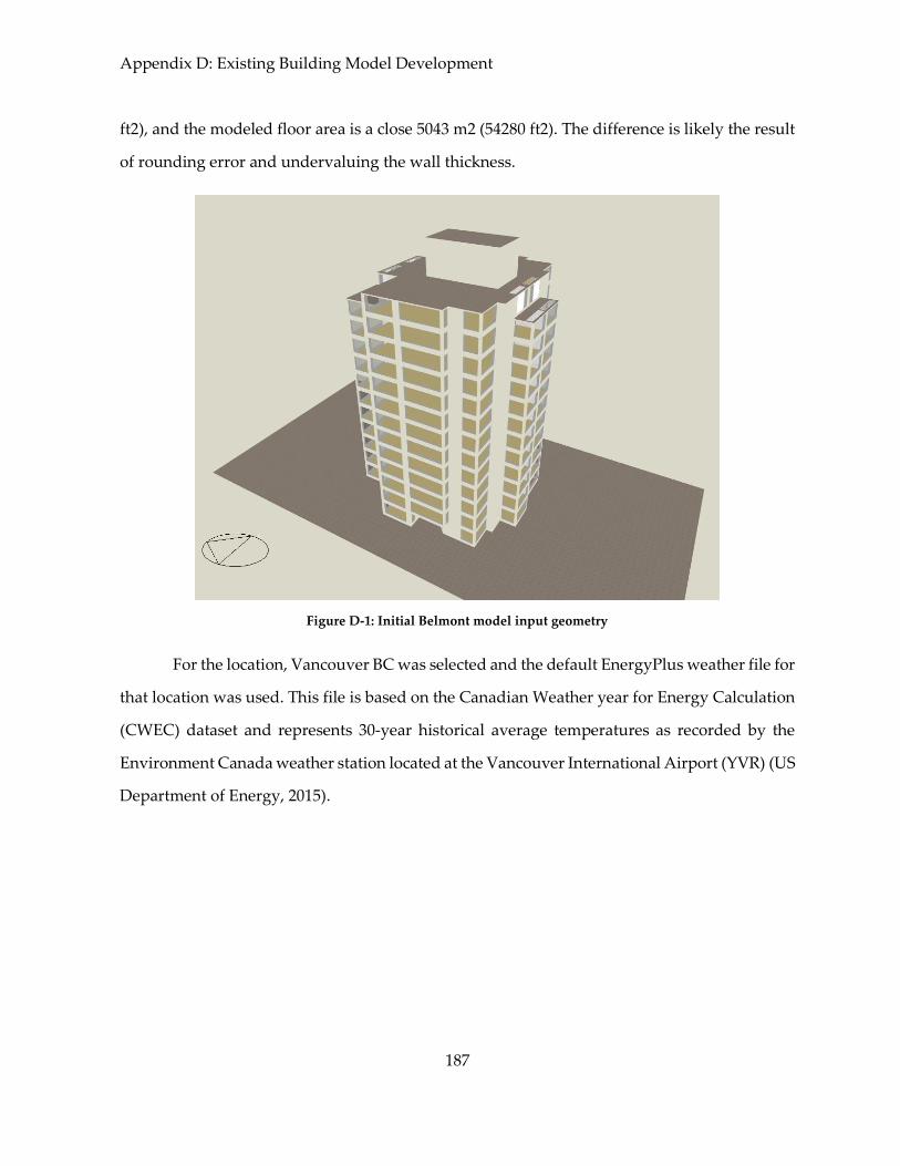
Appendix D: Existing Building Model Development
187
ft2), and the modeled floor area is a close 5043 m2 (54280 ft2). The difference is likely the result
of rounding error and undervaluing the wall thickness.
Figure D-1: Initial Belmont model input geometry
For the location, Vancouver BC was selected and the default EnergyPlus weather file for
that location was used. This file is based on the Canadian Weather year for Energy Calculation
(CWEC) dataset and represents 30-year historical average temperatures as recorded by the
Environment Canada weather station located at the Vancouver International Airport (YVR) (US
Department of Energy, 2015).

Appendix D: Existing Building Model Development
188
Figure D-2: Initial Belmont model typical floorplan
D.1.2 Constructions and Openings
The key assemblies in an energy model are those that comprise the enclosure as they act
as an environmental separator and have a direct impact on the building heating and cooling
loads. For The Belmont, these constitute the above grade walls, the roof and decks, the below
grade walls, the ground floor, and the windows and doors. Internal floors and internal partition
walls also need to be defined however as they impact heat flow between internal zones.
One of the challenges associated with defining the constructions is that the user must
input the assemblies as layers of predefined materials, and the insulation value is then
calculated based on one-dimensional heat flow. The problem with this approach is that often
the effective three-dimensional heat flow differs considerably from the one-dimensional
analysis due to thermal bridging, thermal flanking, and other three-dimensional phenomena.
In order to input the correct R-value for each assembly, it was therefore necessary to modify the
thicknesses of certain layers to decrease the nominal value. For thermal purposes this practice
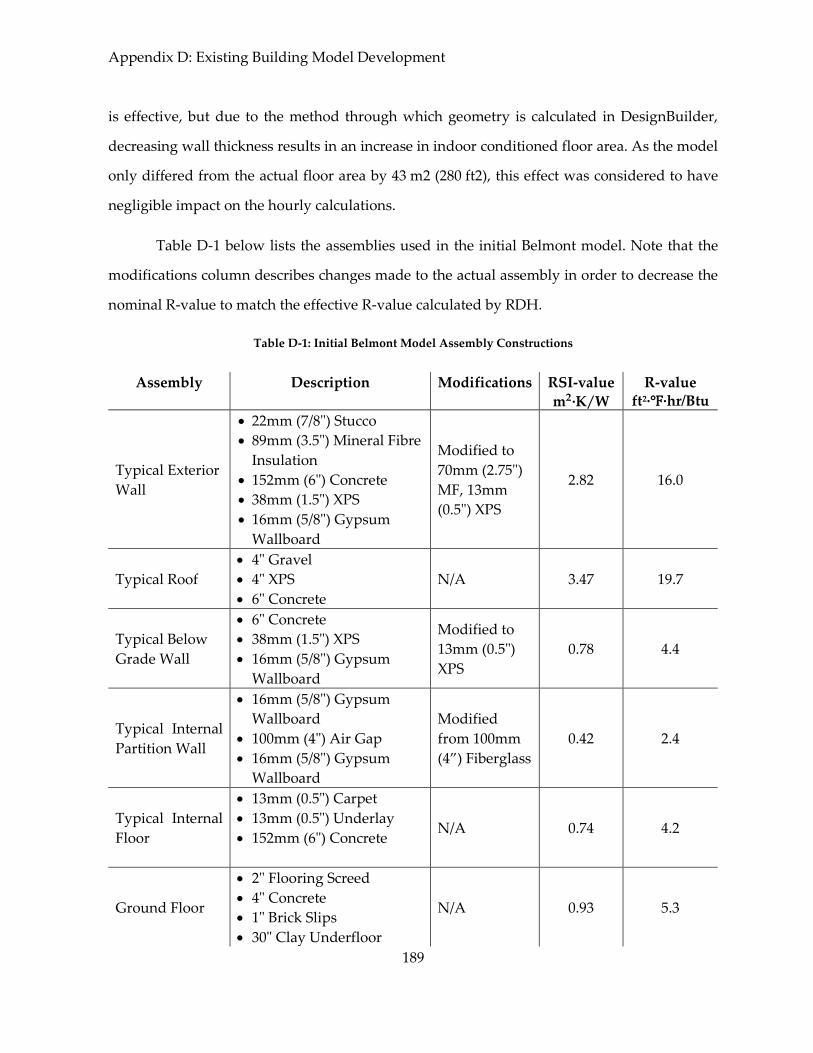
Appendix D: Existing Building Model Development
189
is effective, but due to the method through which geometry is calculated in DesignBuilder,
decreasing wall thickness results in an increase in indoor conditioned floor area. As the model
only differed from the actual floor area by 43 m2 (280 ft2), this effect was considered to have
negligible impact on the hourly calculations.
Table D-1 below lists the assemblies used in the initial Belmont model. Note that the
modifications column describes changes made to the actual assembly in order to decrease the
nominal R-value to match the effective R-value calculated by RDH.
Table D-1: Initial Belmont Model Assembly Constructions
Assembly Description Modifications RSI-value
m2∙K W⁄
R-value ft2∙℉∙hr/Btu
Typical Exterior
Wall
22mm (7/8") Stucco
89mm (3.5") Mineral Fibre
Insulation
152mm (6") Concrete
38mm (1.5") XPS
16mm (5/8") Gypsum
Wallboard
Modified to
70mm (2.75")
MF, 13mm
(0.5") XPS
2.82 16.0
Typical Roof
4" Gravel
4" XPS
6" Concrete
N/A 3.47 19.7
Typical Below
Grade Wall
6" Concrete
38mm (1.5") XPS
16mm (5/8") Gypsum
Wallboard
Modified to
13mm (0.5")
XPS
0.78 4.4
Typical Internal
Partition Wall
16mm (5/8") Gypsum
Wallboard
100mm (4") Air Gap
16mm (5/8") Gypsum
Wallboard
Modified
from 100mm
(4”) Fiberglass
0.42 2.4
Typical Internal
Floor
13mm (0.5") Carpet
13mm (0.5") Underlay
152mm (6") Concrete
N/A 0.74 4.2
Ground Floor
2" Flooring Screed
4" Concrete
1" Brick Slips
30" Clay Underfloor
N/A 0.93 5.3
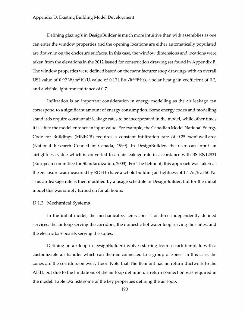
Appendix D: Existing Building Model Development
190
Defining glazing’s in DesignBuilder is much more intuitive than with assemblies as one
can enter the window properties and the opening locations are either automatically populated
are drawn in on the enclosure surfaces. In this case, the window dimensions and locations were
taken from the elevations in the 2012 issued for construction drawing set found in Appendix B.
The window properties were defined based on the manufacturer shop drawings with an overall
USI-value of 0.97 W/m2 K (U-value of 0.171 Btu/ft2∙℉∙hr), a solar heat gain coefficient of 0.2,
and a visible light transmittance of 0.7.
Infiltration is an important consideration in energy modelling as the air leakage can
correspond to a significant amount of energy consumption. Some energy codes and modelling
standards require constant air leakage rates to be incorporated in the model, while other times
it is left to the modeller to set an input value. For example, the Canadian Model National Energy
Code for Buildings (MNECB) requires a constant infiltration rate of 0.25 l/s/m2 wall area
(National Research Council of Canada, 1999). In DesignBuilder, the user can input an
airtightness value which is converted to an air leakage rate in accordance with BS EN12831
(European committee for Standardization, 2003). For The Belmont, this approach was taken as
the enclosure was measured by RDH to have a whole building air tightness of 1.4 Ac/h at 50 Pa.
This air leakage rate is then modified by a usage schedule in DesignBuilder, but for the initial
model this was simply turned on for all hours.
D.1.3 Mechanical Systems
In the initial model, the mechanical systems consist of three independently defined
services: the air loop serving the corridors, the domestic hot water loop serving the suites, and
the electric baseboards serving the suites.
Defining an air loop in DesignBuilder involves starting from a stock template with a
customizable air handler which can then be connected to a group of zones. In this case, the
zones are the corridors on every floor. Note that The Belmont has no return ductwork to the
AHU, but due to the limitations of the air loop definition, a return connection was required in
the model. Table D-2 lists some of the key properties defining the air loop.

Appendix D: Existing Building Model Development
191
Table D-2: Initial Belmont model – air loop properties
Property Value Notes
Design Flow Rate 1557 l/s
(3300 cfm)
From drawings, verified by
field testing performed by
RDH
Supply Fan External Static
Pressure
250 Pa
(1” H2O) From drawings
Supply Fan Efficiency 70% Assumption
Corridor Mechanical Ventilation 3.136 Ac/h
Based on design flow rate
divided by volume of
corridors
Heating Coil Capacity 73.2 kW (250 MBH) Coil rated input from
drawings
Coil Part Load Curve Standard Gas Coil PLC DesignBuilder default
Heating Fuel Source Natural Gas Known
Heating Burner Efficiency 80% From drawings
Air Loop Setpoint Schedule Air Loop Heating
Schedule – Always 35°C DesignBuilder default
Corridor Heating Setpoint 18°C (64.4°F) Known from monitoring
Unit Availability Schedule Always On Known
Corridor Ventilation Schedule Always On Known
Similarly to the air loop, defining a domestic hot water loop involves starting from an
initial template containing a customizable water heater and pump which can then be connected
to water outlet zones. In this case, the outlet zones are the suites as further resolution of
bathrooms and kitchens was not built into this initial model. Table D-3 lists some of the key
properties defining the domestic hot water loop. Note that the demand is based on the
recommended design value of 0.15 m3 suite/day⁄ (40 US Gallons suite/day⁄ ) set by ASHRAE
90.1-2004 for multifamily buildings rather than the estimated values discussed in section 3.2.5
(American Society of Heating Refrigerating and Air-Conditioning Engineers, 2004).
Additionally, the usage schedule was taken from the Model National Energy Code for
Buildings (MNECB), and can be found along with all of the other schedules used in Appendix
C (National Research Council of Canada, 1999).

Appendix D: Existing Building Model Development
192
Table D-3: Initial Belmont model – domestic hot water loop properties
Property Value Notes
Water Loop Flow Variable Flow DesignBuilder default
Water Heater Tank Volume Autosize Calculated by
DesignBuilder
Setpoint Temperature DHW setpoint schedule
– always 55°C DesignBuilder default
Heating Fuel Source Natural Gas Known
Boiler Heating Capacity 178.7 kW (610 MBH) From equipment boiler
plate
Heating Thermal Efficiency 82.4% From equipment boiler
plate
Heater Part Load Factor Curve
Newer Style Moderate
Temperature Boiler
circa 1983
Selected from
DesignBuilder templates
based on year of
construction
Pump Rated Power Consumption Autosize Calculated by
DesignBuilder
Pump Speed Variable DesignBuilder default
Rated Pump Head 20 kPa
(6.691 Ft H2O) DesignBuilder default
Pump Performance Curve Constant Output (no
variable speed) DesignBuilder default
Pump Control Strategy Intermittent DesignBuilder default
DHW Demand 40 Gal/Day/Apartment From ASHRAE 90.1-2004
User’s Manual
DHW Suite Load 0.03031 Gal/ft2/day
Based on ASHRAE 90.1 and
the total apartment floor
area within the model. This
value is only applied to the
suite floor area
DHW Demand Schedule MNECB-1999
Multifamily DHW
Assumption
See Appendix C
Water Heater Availability
Schedule Always On Known
Baseboard Convectors were added to each suite as the heating system, powered by
electricity using a heating coefficient of performance (COP) of 1.0. Note that DesignBuilder also

Appendix D: Existing Building Model Development
193
offers baseboard radiators, but as the majority of heat transferred from modern electric
baseboards is in the form of convection, baseboard convectors were selected instead.
Additionally, while the heating setpoints are not known, a setpoint of 22°C (71°F) was taken
based on the House Simulation Protocols produced by the US National Renewable Energy
Laboratory (Wilson et al., 2014). Table D-4 list some of the key properties associated with the
electric baseboards.
Table D-4: Initial Belmont model – electric baseboard properties
Property Value Notes
Typical Suite Capacity Autosize Calculated by
DesignBuilder
Heating Fuel Electricity Known
Heating COP 1.0 Known
Heating Setpoint Temperature 22°C (71°F) Assumption from NREL
House Simulation Protocols
Heating Setback None Assumption from NREL
House Simulation Protocols
D.1.4 Lighting, Gains and Occupancy
Internal gains from lighting, occupants, and miscellaneous equipment are crucial in
determining the energy use of a building as they both use energy directly as well as offset the
heating load which must be met by the HVAC system. The difficulty with these gains in the
context of The Belmont specifically is that not very much information is available, and so one
must rely on default values and generalized inputs from energy codes and modeling standards.
Lighting was broken down into three distinct areas: the parkade, the suites, and the
corridors. Lighting intensities were taken from ASHRAE Standard 90.1-2007 using the building
area method for multifamily buildings and parking garages, and the suites and parkades were
therefore treated as one (American Society of Heating Refrigerating and Air-Conditioning
Engineers, 2007). The lighting schedules were taken from MNECB-1999, which can be found

Appendix D: Existing Building Model Development
194
along with all other schedules used in Appendix C (National Research Council of Canada,
1999).
For MURBs, DesignBuilder defaults to include stepped lighting controls to mimic
occupant control with respect to daylighting in the suites. This means that for a given time step,
the illuminance of a space due to daylight is calculated and compared to the target illuminance.
The discrete steps involved with stepped lighting control simulate turning specific fixtures on
or off in order to meet the illuminance target, as opposed to simply turning all of the zone
lighting on. In DesignBuilder, the default target illuminance of 300 Lux was used for all spaces.
Table D-5 displays some key inputs associated with the lighting properties in the three
main areas of The Belmont model. Note that all other lighting parameters were left at the
DesignBuilder default values, which are listed in Table 3-8.
Table D-5: Initial Belmont model – lighting properties
Property Suites Corridors Parkade
Lighting Power Density 6.5 W/m2 0.6 W/ft2
6.5 W/m2 0.6 W/ft2
2.7 W/m2 0.25 W/ft2
Target Illuminance 300 Lux 300 Lux 300 Lux
Schedule
MNECB-1999
Multifamily
Lighting
On On
Lighting Controls
Stepped with 3
steps to mimic
occupant behavior
N/A N/A
In The Belmont, there are two main internal equipment gains: miscellaneous electrical
equipment in suites, and natural gas fireplaces in suites on floors 9 through 13. To simplify the
initial model, the fireplaces were not included. For the miscellaneous electrical equipment, a
similar difficulty to the lighting exists in that not much information is available about the types
of equipment and appliances present in each suite. As such, the MNECB-1999 value of 5 W/m2
(0.4645 W/ft2) was used along with the corresponding MURB miscellaneous electrical load
schedule (National Research Council of Canada, 1999). No equipment electrical gain was

Appendix D: Existing Building Model Development
195
included for the corridors or parkade in order to simplify the initial model, although some
equipment is present there such as the elevators and parkade exhaust fans. Table D-6 lists some
of the key properties associated with the equipment gains.
Table D-6: Initial Belmont model – miscellaneous equipment properties
Property Value Notes
Typical Suite Equipment Gain 5 W/m2
(0.4645 W/ft2) From MNECB-1999
Equipment Fuel Electricity Known
Equipment Schedule MNECB-1999
Multifamily receptacle From MNECB-1999
Radiant Fraction 0.2 DesignBuilder default
The Belmont, as previously discussed, is inhabited by individuals of at least 55 years or
older. The majority of suites are 2 bedrooms, but are occupied by 1 or 2 individuals. The
occupant density and metabolic considerations were based on DesignBuilder defaults for
MURBs, however they are roughly correct based on what limited information is available about
the occupants. The occupant schedule was based on MNECB-1999 as a starting point for the
initial model, but as most occupants are retired the traditional workday assumptions inherent
in residential schedules don’t necessarily apply (National Research Council of Canada, 1999).
Table D-7 displays some key properties associated with the occupancy. Note that these
properties only apply to the suites, as the corridors and parkade are considered to be
unoccupied.
Table D-7: Initial Belmont model – occupancy properties
Property Value Notes
Typical Suite Occupant Density 0.02 People/m2
(0.001858 People/ft2) DesignBuilder default
Occupancy Schedule MNECB-1999
Multifamily occupancy From MNECB-1999
Metabolic Activity Level Typing DesignBuilder default
Winter Clothing 1.0 clo DesignBuilder default
Summer Clothing 0.5 clo DesignBuilder default

Appendix D: Existing Building Model Development
196
D.1.5 Initial Modelled Energy Consumption
Given the inputs and assumptions described in Sections C.1.1 through C.1.4, the annual
energy consumption of the Belmont initial model was calculated by DesignBuilder using
EnergyPlus 8.4. Figure D-3 displays the modelled electricity consumption with respect to the
metered consumption from BC Hydro in 2013. Note that as the typical meteorological year
weather file was used in the models, an exact match was not expected from the initial model.
However, some clear discrepancies are visible.
Figure D-3: Initial Belmont model – monthly electricity consumption
From Figure D-3, it is clear that the model is dramatically under predicting the electricity
consumption. The under prediction of baseline consumption in the summer months indicates
that the base lighting or electrical equipment gain needs to be increased. Additionally, the lack
of seasonal variation with respect to the metered consumption indicates that the suite electric
heating is not being fully captured.
Figure D-4 displays the modelled natural gas consumption with respect to the metered
consumption from Fortis BC for 2013. The initial model is dramatically over predicting the
natural gas consumption – particularly in the summer months where the modelled
consumption is more than twice the metered consumption.
0
5000
10000
15000
20000
25000
30000
35000
40000
45000
50000
Jan-13 Feb-13 Mar-13 Apr-13 May-13 Jun-13 Jul-13 Aug-13 Sep-13 Oct-13 Nov-13 Dec-13
Ele
ctri
city
Co
nsu
mp
tio
n, k
Wh
Month
Metered, 2013 Modelled, TMY

Appendix D: Existing Building Model Development
197
Figure D-4: Initial Belmont model – monthly natural gas consumption
A better understanding of how the model is calculating the energy consumption can be
gleaned by analyzing the annual end-use consumption as seen in Figure D-5 in contrast with
the estimated end-use consumption presented in Figure 3-17. To simplify the comparison, an
annual summary by end use is presented in Figure D-6. Several of the end-uses are not being
accurately simulated; The model is under predicting the baseboard heating electricity by
approximately 75%. The domestic hot water is being under predicted by approximately 25%.
As limited sub-metering was available in the metered energy analysis, it is difficult to ascertain
whether or not the equipment and lighting loads are correct, but given the small values
simulated for pumps and fans it is likely that those two specific equipment categories are not
properly configured. Lastly, the make-up air unit gas consumption is almost 300% higher than
the estimated consumption, indicating that one or more of the input assumptions associated
with the air loop must be invalid.
0
10000
20000
30000
40000
50000
60000
70000
80000
Jan-13 Feb-13 Mar-13 Apr-13 May-13 Jun-13 Jul-13 Aug-13 Sep-13 Oct-13 Nov-13 Dec-13
Gas
Co
nsu
mp
tio
n,
kW
h
Month
Metered, 2013 Modelled, TMY

Appendix D: Existing Building Model Development
198
Figure D-5: Initial Belmont model – annual end-use consumption
Figure D-6: Initial Belmont model – annual end-use consumption – modelled consumption vs estimates from
monitoring data
Beyond the modeled energy consumption itself, an interesting observation can be made
surrounding the calculated air change rate from natural ventilation, mechanical ventilation and
infiltration. On average the simulation showed 0.58 air changes per hour for the whole building,
Room Electricity
(kWh), 87,758 , 9%
Lighting (kWh),
145,256 , 15%
System Fans (kWh),
4,849 , 1%
System Pumps
(kWh), 15 , 0%
Heating (Electricity)
(kWh), 25,875 , 3%Heating (Gas)
(kWh), 556,211 ,
58%
DHW (Gas) (kWh),
134,447 , 14%
0 100,000 200,000 300,000 400,000 500,000 600,000
Heating - Gas (MAU)
Domestic Hot Water - Gas
Fireplaces - Gas
Heating - Elec (Suites)
Lighting & Equip (Suites)
Lighting & Equip (Common)
Annual Energy Consumption, kWh
En
d-U
se C
ateg
ori
es
Estimated from Monitoring Modelled

Appendix D: Existing Building Model Development
199
with minimal variation throughout the entire year. This is not entirely consistent with the
measured air change rate of 0.4-0.5 ac/h measured by RDH using tracer gas testing in April 2013
(Ricketts, 2014).
D.2 Second Pass Energy Model
While the initial model served as a first attempt at accurately simulating the Belmont,
the results discussed in Section C.1.5 indicated several large discrepancies between the
measured and modelled building performance. As such, the second pass model serves to
address invalid initial assumptions and add additional detail to aspects of the model identified
as potentially having significant contributions to the building energy use. The second pass
model calibrations are based on additional known details and founded assumptions largely
implemented to replace DesignBuilder default values and initial model simplifications.
D.2.1 Second Pass Model Calibrations
Calibrations to the initial Belmont model include changes to building geometry,
mechanical systems, and internal gains. Table D-8 lists the calibrations in the order which they
were applied. Note that in discussions of the energy impacts, each calibration is considered
sequentially with discussed changes in energy consumption taken with respect to the previous
model iteration.
Table D-8: List of second pass Belmont model calibrations in sequential order
Second Pass
Iteration Calibration
2.1 Modified internal layout to reflect actual floorplan
2.2 Adjusted DHW load to only apply to spaces containing hot water outlets
2.3 Adjusted the MAU delivery setpoint temperature
2.4 Added bathroom and kitchen mechanical ventilation
2.5 Added natural ventilation to account for open windows
2.6 Added fireplaces to the living rooms of suites on the top 5 floors

Appendix D: Existing Building Model Development
200
Second Pass
Iteration Calibration
2.7 Added parkade ventilation and elevator energy consumption
2.8 Changed domestic hot water pump settings to more realistic estimates
2.9 Changed the weather file to the 2013 Vancouver meteorological year
D.2.1.1 Calibration 2.1: Internal Layout
The first calibration involved subdividing the internal layout of each suite. Although
not explicitly required, this was done in an attempt to add further resolution and accuracy to
the model. Figure D-7 displays the new typical floor plan, which can be contrasted with Figure
D-2 in Section D.1.1.
Figure D-7: Second Pass Belmont model typical floorplan

Appendix D: Existing Building Model Development
201
As part of changing the internal layout, some of the window locations needed to be
adjusted slightly such that there was no overlap between the fenestration location and interior
wall to exterior wall connections. Otherwise, all of the other inputs were left the same as the
initial model.
In comparison to the initial model results, there were several slight variations in end-
use consumption with the subdivided internal layout. Firstly, the miscellaneous electrical load
decreased by around 4200 kWh or 5% annually. This can be attributed to the fact that equipment
loads are defined in power per unit floor area, and as the internal partition walls have finite
dimensions, the effective floor area of each unit decreased slightly. A similar result was
observed with respect to the domestic hot water, which is also defined per unit area and
decreased by about 7000 kWh or 5% annually. Conversely, the lighting energy increased
slightly by around 2000 kWh or 1% annually. This is likely due to the fact that the lighting
controls in the suites account for daylighting, and with the internal partition walls numerous
spaces see little or no daylight – requiring more lighting energy. Overall, the total change with
respect to the initial model was around 8000 kWh or a 0.8% decrease annually. While this is
non-trivial, it is fairly insignificant and was therefore deemed acceptable.
D.2.1.2 Calibration 2.2: Domestic Hot Water
With the internal layout of each suite divided into specific rooms, it is possible to
redefine the domestic hot water load to reflect only the spaces which contain hot water outlets.
This is also necessary as the initial DHW input of 0.03031 Gal/ft2/day discussed in Table D-3
was based on the initial model suite floor areas, and the new suite floor areas are slightly
smaller.
In keeping with the original assumption of 40 gallons per day per apartment from
ASHRAE 90.1-2004, a new load of 0.1354 Gal/ft2/day was assigned based on the new floor areas
of only the bathrooms and kitchens with the intent of replicating the initial domestic hot water
use observed in Section D.1.5 (American Society of Heating Refrigerating and Air-Conditioning
Engineers, 2004).

Appendix D: Existing Building Model Development
202
On an annual basis, the domestic hot water load increased by around 6300 kWh or 5%
as compared the previous model iteration, resulting in an annual domestic hot water energy
use of around 134,000 kWh. This annual consumption, while an increase from the previous
model iteration, is very similar to the initial domestic hot water consumption discussed in
Section D.1.5 and the insignificant differences can be attributed to rounding error.
D.2.1.3 Calibration 2.3: Makeup-Air Unit Setpoint Temperature
One of the most visible inaccuracies of the initial model annual energy consumption
results had to do with the makeup air unit natural gas consumption. This excessive
consumption can be attributed to the fact that the setpoint temperature was left at the air loop
heating default value of 35°C. In reality, the corridor ventilation air is only conditioned to 18-
20°C, and this extra 15°C of conditioning at all times resulted in a substantial amount of energy
given that the MAU constantly provides 1557 l/s (3300 cfm) of fresh air.
Changing the setpoint temperature to 18°C resulted in a 358,000 kWh decrease in annual
ventilation heating energy used by the MAU. This 64% decrease in gas heating energy resulted
in a 32,000 kWh increase in space heating energy to account for the fact that less heating energy
was entering the suites from the corridors. Overall, the total annual energy consumption of the
building decreased by 327,000 kWh or 34%.
D.2.1.4 Calibration 2.4: Kitchen and Bathroom Mechanical Ventilation
With the added resolution provided by the subdivided internal layout, it was possible
to include previously overlooked mechanical equipment – in this case, the kitchen and
bathroom exhaust ventilation fans.
In each suite, there are two bathrooms each containing a 33 l/s (70 cfm) exhaust fan
which is operated only when activated by occupants as a form of point exhaust for pollutant
control. As such, exhaust fans were added, but with a capacity of 24 l/s (50 cfm) at 125 Pa static
pressure due to the fact that installed fans typically observe lower than rated airflow due to
inadequate rated static pressures to overcome friction losses in ductwork (Canadian Mortgage

Appendix D: Existing Building Model Development
203
and Housing Corporation, 2003). Additionally, the fan flow rates in a number of units were
measured using a balometer, and while the flow rates varied significantly, 24 l/s is generally
representative of current performance (Ricketts, 2014). Based on the average bathroom volume
of 22 m3 (760 ft3), this results in 3.94 ac/h for the bathrooms when the fans are operating.
In terms of a bathroom fan operating schedule, little guidance is available through
standards. The NREL House Simulation Protocols assume that bathroom fans, when operating
as point exhaust, are only on for an hour per day which can be simulated between 7 and 8am
(Wilson et al., 2014). While not intended for use in high-rise MURBs, this assumption is still
valid and was therefore implemented in the Belmont model.
For the kitchen exhaust, no information about fan capacity was provided through site
visits or mechanical drawings. As such, the DesignBuilder default value of 100 l/s (211 cfm) at
125 Pa static pressure was retained as this is a reasonable capacity for a kitchen exhaust hood.
Based on the average kitchen volume of 31 m3 (1100 ft3), a flow rate of 11.5 ac/h is achieved
when the fan is operating. As with the bathrooms, no information was available to dictate the
kitchen operating schedule, but the NREL guidelines recommend modelling the kitchen fans
as operating for one hour a day between 6-7pm (Wilson et al., 2014).
On an annual basis, these additional fans increased the building fan energy
consumption by 9400 kWh, which is a 193% increase from previous model iterations. This is to
be expected as all of these fans were previously unaccounted for. This increased consumption
corresponds to a 1.5% increase in total annual energy consumption.
D.2.1.5 Calibration 2.5: Natural Ventilation
One of the unique characteristics of high-rise multi-unit residential buildings which sets
them apart from other high-rise construction is the abundance of operable windows and doors
for natural ventilation. This was not included in the initial model, but it seemed a necessary
inclusion for improved model accuracy.

Appendix D: Existing Building Model Development
204
As with the bathroom and kitchen exhaust ventilation, little guidance was available
with how to model natural ventilation explicitly, so assumptions were needed. It was assumed
that when the indoor temperature is above 22°C (72°F), the occupants would open the windows
resulting in 3 ac/h of outdoor ventilation air. While the 3 ac/h was a DesignBuilder default value,
the indoor temperature setpoint was taken from the NREL house simulation protocols (Wilson
et al., 2014).
The addition of natural ventilation had a notable impact on electric baseboard heating
energy, increasing it by 12,000 kWh or 20% annually. Proper implementation of natural
ventilation would stipulate that the indoor minimum temperature setpoint should be raised to
avoid windows being open when heating is required, but as some occupants will likely have
their windows open during these periods regardless, the result was deemed acceptable. In
addition to the change in energy consumption, the whole building air change rate increased.
Previously, the modelled air change rate was around 0.38-0.4 ac/h on average throughout the
year, the building air change rates increased up to 1.4 ac/h during the summer months.
D.2.1.6 Calibration 2.6: Fireplaces
The natural gas fireplaces were omitted from the initial model as they are only present
in the living rooms of suites on the top 5 floors, and they are intended to be used as a luxury
item as opposed to a space heating device. However, as identified in the measured energy
consumption analysis, the fireplaces constitute a considerable amount of the annual building
energy consumption and therefore should be accounted for in the model.
The typical fireplace unit installed in The Belmont suites has a capacity of 8.8 kW (30,000
Btu/h) as discussed in section 3.1.3. Based on the average living room area of the suites on the
top 5 floors, this results in a space gain of 1.4 W/m2 (15 W/ft2) to the living rooms when the
fireplaces are operating. As gas fireplaces tend to transmit most of their heat as radiation, and
typically only achieve efficiencies of 50-70%, the radiant fraction of the gain was set to 0.6. The
fraction lost set to 0.4 in order to account for the energy lost through the flue.

Appendix D: Existing Building Model Development
205
Determining the fireplace usage schedule was difficult as the fuel consumption was not
measured, but rather the temperature of the baseplate adjacent to the pilot light. A number of
assumptions were inherent in determining the times during which the units were on as
discussed in Section 3.2.3. The fireplace scheduled monthly hour of operation from all units can
be seen in Figure D-8 along with the estimated hours of operation from the monitoring data.
Note that in order to simplify the creation of daily and weekly schedules, the hours of operation
were only approximated.
Figure D-8: Second pass Belmont model fireplace monthly hours of operation vs. estimated monthly hours of
operation from monitoring data. Values represent the total for all fireplace units in The Belmont
The actual fireplace schedule implemented in DesignBuilder needed to have a higher
resolution than presented in Figure D-8. Based on the monthly hours of operation, weekly and
daily schedules were created in order to capture the approximate total number of hours on
while also applying the loads at realistic times during the day. Table D-9 displays the daily
scheduled hours of operation, which were chosen to coincide with periods of occupancy.
0
500
1000
1500
2000
2500
3000
Fir
epla
ce M
on
thly
Ho
urs
of
Op
erat
ion
fro
m a
ll u
nit
s
Month
Estimated Hours "On" from monitoring data
Approximated hours "On" for use in model

Appendix D: Existing Building Model Development
206
Table D-9: Second pass Belmont model – fireplace schedule
Month Weekdays Weekends Monthly Hours
“On” per Fireplace
January 5pm – 10pm 12pm – 8pm 179
February 5pm – 10pm 12pm – 8pm 164
March 7pm – 10pm 4pm – 8pm 103
April 7pm – 10pm 4pm – 8pm 98
May 9pm – 10pm N/A 23
June 9pm – 10pm N/A 20
July N/A 9pm – 10pm 8
August N/A 9pm – 10pm 9
September N/A 9pm – 10pm 9
October 9pm – 10pm N/A 23
November 7pm – 10pm 4pm – 8pm 99
December 5pm – 10pm 12pm – 8pm 182
As no room gas load previously existed in the model, adding the fireplaces represented
a significant increase of around 103,000 kWh per year. All of this additional heat did correspond
in space heating gains however, and as such the suite electrical heating energy consumption
decreased by around 15,700 kWh or 22%. This decrease is larger than expected, but the suite
heating energy is still under modelled which is resulting in a disproportionately large
percentage decrease. On an annual basis, the total building energy consumption increased by
around 86,000 kWh or 13%.
D.2.1.7 Calibration 2.7: Parkade and Elevator Loads
The initial model did not include any equipment loads for the parkade or the elevator
machine room, despite the fact that the parkade contains large exhaust fans and the elevator
machine room contains the elevator motors. As these are both electrical equipment loads, and

Appendix D: Existing Building Model Development
207
the initial model under predicted the baseline electrical consumption, the parkade and elevator
mechanical equipment gains seemed a necessary addition.
The parkade contains two 4800 l/s (10,200 cfm) exhaust fans which operate with an
external static pressure of 31 Pa (1/8” water column). Based on the volume of the parkade, the
space receives a ventilation rate of 5.4 ac/h with the fans fully operational. As the parkade
exhaust fan schedule is unknown but ventilation is likely always required, the fans were simply
set to operate at all times.
For the elevator machine room, determining the equipment load was difficult given the
lack of information. DesignBuilder has a default template for elevator machine rooms, but the
16 W/m2 lighting intensity and the 4000 W/m2 equipment gains seemed unrealistic for this
application. The lighting was left off as the space is very small and typically unoccupied. The
equipment load was estimated to fall somewhere between an infrequently operated low-rise
elevator of 1900 kWh/year and a frequently operated high-rise elevator at 15,000 kWh/year
(Sachs, 2005). It was assumed that the Belmont consumption falls in between these two
extremes at around 8500 kWh/year. This load was divided by the area of the elevator machine
room and the hours of the year to get a load of 21.5 W/m2 (2 W/ft2). While the true hours of
operation are unknown, it is unlikely that the elevator is ever deactivated aside for
maintenance, and so the constant application of the load is acceptable.
The additional parkade ventilation resulted in a 4400 kWh increase in annual fan energy
– 31% more than modelled in the previous iteration. The added elevator machine room
equipment load increased the miscellaneous electric load by 8500 kWh or 10% annually, but
this added head decreased the space heating electricity slightly by 1200 kWh or 2%. The total
annual building energy consumption therefore increased by 11,600 kWh or 1.6%.
D.2.1.8 Calibration 2.8: Domestic Hot Water Pump Specifications
All previous simulations modelled pump power consumption of only 16 kWh annually.
This consumption corresponds to the only pump in the model which is associated with the

Appendix D: Existing Building Model Development
208
domestic hot water loop. The true consumption of the pump is not known, but the minimal
value suggests that the input assumptions are not valid despite the fact that all pump
specifications were left at DesignBuilder defaults. Three invalid assumptions were identified
and addressed individually: the pump speed, the control strategy, and the pump head pressure.
The domestic hot water loop flow type and pump speed are tied together in
DesignBuilder, and can either be set to constant flow with a constant speed pump or variable
flow with a variable speed pump. The default values involve variable flow and speed, but given
the vintage of the Belmont, the pump is most likely constant speed. The flow and pump speed
were therefore changed to constant, and rather than utilizing an autosized flow rate, the
maximum flow rate was set to the known design value of 0.63 l/s (10 gpm).
The default pump control strategy is intermittent which implies that the pump cycles
on and off depending on demand. This is also unlikely given the vintage of the Belmont, and
was therefore changed to constant operation.
The domestic hot water recirculation pump serves to circulate the water throughout the
building, and to facilitate flow to the mechanical penthouse where the boiler and water heaters
are located. As this is an open loop, the pump must overcome a physical change in height,
meaning that the default head pressure of 20 kPa (6.7 ft H2O) is dramatically insufficient. From
the original Belmont drawings, the pump head is 75 kPa (25 ft H2O), and so the model inputs
were changed accordingly. Additionally, the pump input power was changed from autosize to
the known value of 250 W (1/3 hp).
The new pump configuration increased annual pumping energy by 2160 kWh or
14,270%. While this new estimate still gives pumping the smallest end-use consumption, it is
likely closer to the real consumption than previously modelled. The new control strategy did
however decrease the domestic hot water energy consumption slightly by 3270 kWh, resulting
in an overall decrease in annual energy consumption of 1100 kWh or 0.1%.

Appendix D: Existing Building Model Development
209
D.2.1.9 Calibration 2.9: Vancouver 2013 Meteorological Weather Data
Up to this point, all model iterations have been completed using the Vancouver
International Airport CWEC historically averaged weather file. While this weather data is
statistically representative, it does not reflect the actual weather which was occurring during
the measured consumption period of 2013. To address this, RDH provided the 2013 actual
meteorological year weather file from the Vancouver International Airport for use with
EnergyPlus.
The 2013 weather file differed only slightly from the CWEC historically averaged file,
but the changes were enough to make non-trivial changes to the space conditioning and lighting
energy. The most significant changes were to the ventilation energy, which decreased by 11,300
kWh or 6% as well as the electric baseboard heating electricity which decreased by 9,900 kWh
or 18%. There were however slight increases to the fireplace and lighting energy consumption.
Overall, the total annual energy consumption decreased by 20,200 kWh or 2.7%.
D.2.2 Summary of Second Pass Calibrations
Table D-10 displays the impact of all the sequential calibrations discussed in Section
D.2.1 in terms of the impact each calibration had on the annual total building energy
consumption.
Table D-10: Summary of second pass Belmont model calibrations and their effect on annual energy
consumption
Second
Pass
Iteration
Calibration
Annual Energy
Consumption
kWh
Change from Previous
Model Iteration
kWh %
2.1 Internal Layout 946,371 -8,039 -0.8%
2.2 DHW load 952,715 6,343 0.7%
2.3 MAU Setpoint 626,110 -326,605 -34.3%
2.4 Bath and Kitchen Ventilation 635,490 9,380 1.5%
2.5 Natural Ventilation 643,969 8,480 1.0%
2.6 Fireplaces 729,577 85,607 13.3%

Appendix D: Existing Building Model Development
210
Second
Pass
Iteration
Calibration
Annual Energy
Consumption
kWh
Change from Previous
Model Iteration
kWh %
2.7 Parkade and Elevator Gains 741,152 11,575 1.6%
2.8 DHW pump 740,047 -1,105 -0.1%
2.9 2013 Weather File 719,803 -20,243 -2.7%
D.2.3 Second Pass Modelled Energy Consumption
Combining all of the sequential model calibrations, the final second pass Belmont
energy model provides much more detail with respect to the model representation of available
information about the building. Despite this, the modelled energy consumption still is not
completely consistent with the metered electricity consumption for 2013.
Figure D-9 displays the modelled and metered electricity consumption for 2013 as
recorded by BC Hydro and simulated by the second pass model. As with the initial model, the
baseline electrical consumption is being under modelled in the summer months, and the
seasonal variation from electric baseboard heating and lighting energy is not being fully
captured.
Figure D-10 displays the modelled and metered natural gas consumption as recorded
by Fortis BC and as simulated by the second pass model. Unlike the electricity, the natural gas
now seems to be much closer to the metered consumption – although some months such as
October and November are still under modelled.

Appendix D: Existing Building Model Development
211
Figure D-9: Second pass Belmont model – monthly electricity consumption for 2013
Figure D-10: Second pass Belmont model – monthly natural gas consumption for 2013
Figure D-11 displays the second pass model annual end-use splits. Note that in
comparison to the initial model, the calibrations have improved the model accuracy in a
number of ways. For example, the ventilation energy, DHW, and fireplace energy (displayed
as Room Gas) are all now in the right order of magnitude. However, the heating electricity is
still being under estimated by the model.
0
5000
10000
15000
20000
25000
30000
35000
40000
45000
50000
Jan-13 Feb-13 Mar-13 Apr-13 May-13 Jun-13 Jul-13 Aug-13 Sep-13 Oct-13 Nov-13 Dec-13
Ele
ctri
city
Co
nsu
mp
tio
n, k
Wh
Month
Measured, 2013 Modelled, TMY
0
10000
20000
30000
40000
50000
60000
70000
80000
Jan-13 Feb-13 Mar-13 Apr-13 May-13 Jun-13 Jul-13 Aug-13 Sep-13 Oct-13 Nov-13 Dec-13
Gas
Co
nsu
mp
tio
n,
kW
h
Month
Measured, 2013 Modelled, TMY

Appendix D: Existing Building Model Development
212
Figure D-11: Second pass Belmont model – annual end-use consumption for 2013
Figure D-12 displays the second pass modelled end-use consumption against the
estimated consumption from monitoring data. While most of the end uses are now closer to the
previously discussed estimates, it is clear that some large discrepancies remain. The common
lighting and equipment is still significantly under predicted while the suite lighting and
equipment is slightly over estimated. The suite heating is still insufficient, but the domestic hot
water loads are fairly accurate with the exception of the domestic hot water load which still
needs to be increased.
Room Electricity
(kWh), 91,978 , 13%
Room Gas (kWh),
103,695 , 14%
Lighting (kWh),
147,844 , 21%
System Fans (kWh),
18,601 , 3%
System Pumps
(kWh), 2,177 , 0%
Heating (Electricity)
(kWh), 43,834 , 6%
Heating (Gas)
(kWh), 186,568 ,
26%
DHW (Gas) (kWh),
125,107 , 17%

Appendix D: Existing Building Model Development
213
Figure D-12: Second pass Belmont model – annual end-use consumption – modelled consumption vs.
estimates from monitoring data
With respect to the modelled air change rate, the second pass simulations are much
more representative of the measured 0.4-0.5 ac/h measured in April of 2013 (Ricketts, 2014). A
whole building air change rate of 0.45-0.5 ac/h was simulated during the winter and spring,
with much higher air change rates of up to 1.5 ac/h simulated during the summer due to natural
ventilation.
D.3 Third Pass Energy Model
The second pass energy model of the Belmont represented the best attempt at
replicating the measured energy consumption based on known details and founded
assumptions. The simulated consumption still differed significantly from the measured
consumption, and as such a third pass of calibrations is required. Unlike the previous iteration,
these calibrations are founded on logical arguments and engineering judgement in an attempt
to achieve agreement between the modelled and measured energy consumption.
D.3.1 Third Pass Model Calibrations
The third pass calibrations to the Belmont model are focused on addressing the specific
deficiencies identified in the second pass result comparison to estimated end-use consumption.
0 50,000 100,000 150,000 200,000 250,000
Heating - Gas (MAU)
Domestic Hot Water - Gas
Fireplaces - Gas
Heating - Elec (Suites)
Lighting & Equip (Suites)
Lighting & Equip (Common)
Annual Energy Consumption, kWh
En
d-U
se C
ateg
ori
es
Estimated from Monitoring Modelled

Appendix D: Existing Building Model Development
214
Specifically, calibrations are focused on suite electricity, common electricity, domestic hot water
consumption, and fireplace consumption. The complete list of third pass calibrations can be
seen below in Table D-11. Note that as previously discussed, the calibrations were preformed
and are discussed in sequential order.
Table D-11: List of third pass Belmont model calibrations in sequential order
Third Pass
Iteration Calibration
3.1 Modified suite electrical loads
3.2 Added common miscellaneous electrical loads (MELs)
3.3 Adjusted domestic hot water demand
3.4 Adjusted fireplace base load and operation schedule
3.5 Adjusted temperature setpoints and enclosure airtightness to increase the
baseboard electrical heating load
D.3.1.1 Calibration 3.1: Suite Electrical Loads
As identified in Figure D-12, the modelled suite lighting and equipment loads exceed
the estimated consumption based on utility data; the modelled consumption amounted to
142,000 kWh/year, whereas the estimated consumption from metering was only
100,000 kWh/year. This indicates that between the suite lighting, miscellaneous electrical loads
(MELs), and suite exhaust fans, one or more of the model inputs is too large. As such, all three
inputs need to be re-evaluated individually.
The bathroom and kitchen exhaust fans were simulated to consume 9300 kWh/year
collectively between the 37 suites. This consumption is based on 50 cfm bathroom fans and 210
cfm kitchen fans operating for one hour per day (Wilson et al., 2014). As this amounts to 250
kWh per suite annually, the modelled consumption is within reasonable expectations and is not
the root cause of the excessive simulated energy consumption. The suite exhaust fan inputs
were therefore unmodified.

Appendix D: Existing Building Model Development
215
The suite miscellaneous electrical loads are assumed to be 5 W/m2 (0.4645 W/ft2) from
MNECB-1999, which based on an average modelled suite floor area of 116 m2 (1250 ft2) amounts
to approximately 580 W of installed miscellaneous equipment per apartment (National
Research Council of Canada, 1999). While this resulted in a total annual consumption of 83,000
kWh, 580 W per apartment is fairly realistic given the power demands of modern appliances.
However, this means that of the 100,000 kWh of annual suite lighting and equipment
consumption estimated from metering, 83% is assumed to be equipment related. As this is a
relatively high percentage, the MELs were dropped to the equivalent of 500 W of installed
capacity per suite, or 4.3 W/m2 (0.4 W/ft2).
Assuming that the MELs are correct, the suite lighting consumption must be reduced
from 50,000 kWh/year to 17,000 kWh/year in order to achieve agreement between the modelled
and estimated consumption. The original input was 6.5 W/m2 (0.6 W/ft2) from ASHRAE
Standard 90.1-2007, which based on an the aforementioned average suite floor area results in
750 W of installed and task lighting within each suite (American Society of Heating
Refrigerating and Air-Conditioning Engineers, 2007). While this power draw would be
conceivable if the majority of the fixtures were incandescent, modern compact fluorescent (CFL)
and light emitting diode (LED) fixtures require substantially less power – often achieving
efficacies over four times that of incandescent lamps (Mather, 2014). As such, the reduction in
suite lighting energy is plausible. In order to achieve the 33,000 kWh/year reduction in energy
consumption, the suite lighting power density was lowered to 2.24 W/m2 (0.21 W/ft2).
Implementing these changes had a fairly substantial impact on electrical loads. Room
electricity decreased by 11,600 kWh or 13% annually while baseboard electric heating increased
by 12,100 kWh. Additionally, the lighting energy decreased by 32,100 kWh or 32% annually.
Overall, the annual total energy consumption decreased 31,400 kWh or 4.4%, which achieved
the intent of decreasing the suite energy consumption.

Appendix D: Existing Building Model Development
216
D.3.1.2 Calibration 3.2: Common Electrical Loads
The common electricity consumption represented the single largest discrepancy
between the measured and modelled energy consumption with the model under predicting
consumption by 72,300 kWh annually. As with the suites, the electrical model inputs associated
with the common electricity consumption need to be re-evaluated in order to determine the
source of the discrepancy. End-uses contributing to the common electrical consumption consist
of the DHW pump, MAU and parkade fans, corridor lighting, and parkade lighting.
The DHW pump and MAU fan are modelled to consume a combined 6500 kWh
annually. While this is a relatively small value, it has already been increased within reasonable
limits and likely isn’t responsibly for a substantial portion of the missing 72,300 kWh. As such,
the inputs surrounding the modelled performance of these systems was left unchanged.
The corridor and parkade lighting power densities were assumed to be 6.5 W/m2
(0.6 W/ft2) and 2.7 W/m2 (0.25 W/ft2) respectively based on ASHRAE Standard 90.1-2007
(American Society of Heating Refrigerating and Air-Conditioning Engineers, 2007). As these
are already conservative values, it is unlikely that the missing common electrical consumption
is due to inadequate modelling of the common lighting. As such, the lighting power densities
were unchanged.
It is evident that the source of the missing electrical consumption has not yet been
identified. It could be the result of transformers in the parkade, electrical/telephone closets in
the corridors, and other as-of-yet unaccounted for MELs. However, as no clear source was
identified, it was instead necessary to implement distributed electrical loads in order to match
the metered consumption. The selections were somewhat arbitrary, but the new MELs were
split between the corridors and the parkade. Equipment loads of 4.75 W/m2 (0.4413 W/ft2) and
2 W/m2 (0.1858 W/ft2) were applied to the corridors and parkade respectively.
The added common MELs increased the annual room electricity consumption by
72,800 kWh or 91%, with a minimal decrease in suite baseboard electrical consumption of

Appendix D: Existing Building Model Development
217
5,300 kWh or 9%. The total annual energy consumption increased by 67,400 kWh or 10%, which
is in accordance with the intent to increase common electricity.
D.3.1.3 Calibration 3.3: Domestic Hot Water Demand
The domestic hot water natural gas consumption simulated was 44,600 kWh/year less
than the estimated consumption from monitoring data. The domestic hot water heater was
configured based on the known equipment specifications, so the main assumption associated
with the system is the daily hot water demand per apartment. This was previously modelled to
be 40 Gallons/day/apartment based on ASHRAE Standard 90.1-2004 (American Society of
Heating Refrigerating and Air-Conditioning Engineers, 2004). In order to achieve agreement
between the metered and modelled consumption, the demand was increased to
53 Gallons/day/apartment, which is consistent with the estimated consumption calculated in
section 3.2.5.
The new domestic hot water demand increased DHW natural gas consumption by
41,000 kWh/year or 33%. This increase, while not the precise value desired, is close enough to
be acceptable, and the small variation of 3000 kWh can be attributed to rounding error in the
input value.
D.3.1.4 Calibration 3.4: Fireplace Consumption
The fireplace consumption also differed from the estimated consumption from
monitoring, but in this case there are many more assumptions – particularly with respect to the
fireplace operating schedule – that need to be re-evaluated.
Firstly, the natural gas consumption of each fireplace was modelled based on the known
value of 8.8 kW (30,000 Btu/h) as previously discussed. This is unlikely to be incorrect, however
the fireplaces do implement a standing pilot light which in many suites is likely left on for
substantial portions of the year. This is could be a possible cause for the discrepancy in
modelled in metered fireplace natural gas consumption of 12,000 kWh/year. In order to address

Appendix D: Existing Building Model Development
218
this, an additional process load of 1.8 W/m2 (0.17 W/ft2) was added to the living rooms with
fireplaces.
The fireplace schedule is the result of numerous assumptions as discussed during the
natural gas monitoring data analysis in section 3.2.3. Rather than re-evaluating all of the core
assumptions and developing a new schedule, the existing schedule was reshaped to match the
trends in consumption observed in the natural gas data. Figure D-13 displays the new fireplace
operating schedule as compared to the previous revision. The total number of hours of
operation were roughly retained for consistency between the second and third pass models.
Note that it was assumed that the MAU and DHW loads are correct, and the remaining
inconsistencies in the natural gas comparison are related to the operation of the fireplaces.
Figure D-13: Second pass vs. third pass fireplace schedule hours of operation for all units
The changes to the fireplace schedule and pilot light baseload resulted in an increase of
12,000 kWh/year of natural gas consumption. This increase was the targeted amount, and
confirms that the approximate number of fireplace operating hours was conserved between the
second and third pass models of the schedule. There was a slight decrease of baseboard heating
energy of 900 kWh, resulting in an overall increase in energy consumption of 11,100 kWh/year.
0
500
1000
1500
2000
2500
3000
Jan-13 Feb-13 Mar-13 Apr-13 May-13 Jun-13 Jul-13 Aug-13 Sep-13 Oct-13 Nov-13 Dec-13
Fir
epla
ce M
on
thly
Ho
urs
of
Op
erat
ion
fro
m a
ll u
nit
s
Month
Second Pass Third Pass

Appendix D: Existing Building Model Development
219
D.3.1.5 Calibration 3.5: Baseboard Electric Heating
The previously discussed calibrations involved manipulating input assumptions
associated directly with a specifically identified end-use. In the case of the baseboard electric
heating, however, the consumption has less to do with the equipment itself and more to do with
the space loads simulated within the suites. As such, the heating setpoints, natural ventilation
controls, and infiltration were re-evaluated to achieve agreement between the metered and
modelled consumption data. Note that the building enclosure insulation level and window
characteristics also impact the space load, but as RDH performed the rehabilitation, these values
are well understood and should not be the source of the discrepancy.
The heating setpoints at the Belmont vary from suite to suite, but for the model a value
of 22°C (71°F) was chosen based on literature (Wilson et al., 2014). A significant increase in
setpoint temperature would be difficult to justify, so only a modest increase to 22.2°C (72°F)
was applied.
Natural ventilation in DesignBuilder is controlled by a set air change rate, modified by
an indoor temperature setpoint. In the previous model iterations, a rate of 3 ac/h was applied
at an indoor temperature exceeding 22°C (71°F). NREL recommends that the natural ventilation
setpoint always exceed the heating setpoint by 1°F to prevent simultaneous heating and cooling
during shoulder seasons (Wilson et al., 2014). As such, in accordance with the revised heating
setpoint, the natural ventilation indoor temperature control needed to be increased. However,
some simultaneous heating and cooling is likely to occur in the Belmont, and may be a likely
contribution to the missing electric baseboard consumption observed in previous model
iterations. Therefore, the natural ventilation setpoint was increased by only 0.5°F above the
heating setpoint to a value of 22.5°C (72.5°F).
Infiltration is a function of many input properties including the building enclosure’s air
permeability, wind forces, stack effect, and mechanical pressures. In DesignBuilder, the user
can input an airtightness value which is converted to an air leakage flow rate as discussed in
Section 3.3.2. The value used in previous model iterations was 1.4 ac/h @ 50 Pa based on

Appendix D: Existing Building Model Development
220
airtightness testing performed at the Belmont (Ricketts, 2014). However, despite all of the
calibrations thus far, the baseboard electricity is greatly under predicted by the model –
particularly during the heating season. This indicates that the heat loss from the space is still
too low. As such, the airtightness value was increased until the baseboard consumption
modelled was in adherence with the value estimated from metering. This value was
substantially higher than the measured airtightness at 3.5 ac/h @ 50 Pa. While this may seem
excessive, it is possible that due to the inaccuracy inherent with the process through which
DesignBuilder estimates air leakage from airtightness values, a higher than measured input is
required for realistic results.
The discussed calibrations resulted in an increase in suite heating energy consumption
of 60,000 kWh or 120% annually. While this is substantial within the specific end-use, the overall
annual consumption increased by only 7.5%.
D.3.2 Summary of Third Pass Calibrations
Table D-12 displays the impact of all the sequential calibrations discussed in Section
D.3.1 in terms of the impact each calibration had on the annual total building energy
consumption.
Table D-12: Summary of third pass Belmont model calibrations and their effect on annual energy consumption
Third
Pass
Iteration
Calibration
Annual Energy
Consumption
kWh
Change from Previous
Model Iteration
kWh %
3.1 Suite electrical loads 688,404 -31,399 -4.4%
3.2 Common equipment loads 755,792 67,388 9.8%
3.3 DHW demand 796,722 40,930 5.4%
3.4 Fireplace load and schedule 807,849 11,127 1.4%
3.5 Electric Baseboards 868,100 60,251 7.5%

Appendix D: Existing Building Model Development
221
D.3.3 Third Pass Modelled Energy Consumption
Combining all of the previously discussed third pass calibrations, the new iteration of
the Belmont model now represents the best possible attempt at simulating the observed real
world energy consumption based on available data, founded assumptions, and engineering
judgement.
Figure D-14 displays the third pass model monthly electricity consumption for 2013 as
compared to the metered consumption from BC Hydro. Note that the largest discrepancy now
lies in October with the modelled consumption falling 11% below the metered consumption.
All other months were within 7% of the target value.
Figure D-14: Third pass Belmont model – monthly electricity consumption for 2013
Figure D-15 displays the third pass model monthly natural gas consumption for 2013
as compared to the metered data from Fortis BC. Unlike the electrical data, there are still
several months that fall outside the desired level of agreement, with August reaching 22%
above the measured consumption. However, while this is a large percentage, the finite value
of the difference is only 3,300 kWh which represents 0.7% of the annual natural gas
percentage. Furthermore, the discrepancy is likely due to varying seasonal domestic hot
0
5000
10000
15000
20000
25000
30000
35000
40000
45000
50000
Jan-13 Feb-13 Mar-13 Apr-13 May-13 Jun-13 Jul-13 Aug-13 Sep-13 Oct-13 Nov-13 Dec-13
Ele
ctri
city
Co
nsu
mp
tio
n, k
Wh
Month
Metered, 2013 Modelled, 2013

Appendix D: Existing Building Model Development
222
water demands which are not captured in the model given the limited resolution of the DHW
schedule.
Figure D-15: Third pass Belmont model – monthly natural gas consumption for 2013
On an annual basis, the end-use splits from both electrical and natural gas demands can
be summarized as shown in Figure D-16. Unlike in previous model iterations where the lighting
dominated electrical consumption and the MAU heating coil dominated the natural gas
consumption, the end-use splits are within norms.
Figure D-17 demonstrates the comparison between the third pass modelled end-use
consumption and the end-use estimates from monitoring data developed in Section 3.2.4. All
modelled end-uses are now within 3% of the estimated consumption, with the common lighting
and equipment almost registering an exact match.
0
10000
20000
30000
40000
50000
60000
70000
80000
Jan-13 Feb-13 Mar-13 Apr-13 May-13 Jun-13 Jul-13 Aug-13 Sep-13 Oct-13 Nov-13 Dec-13
Gas
Co
nsu
mp
tio
n,
kW
h
Month
Metered, 2013 Modelled, 2013

Appendix D: Existing Building Model Development
223
Figure D-16: Third pass Belmont model – 2013 annual end-use splits
Figure D-17: Third pass Belmont model – annual end-use consumption – modelled consumption vs.
estimates from monitoring data
Figure D-18 and Figure D-19 display the monthly simulated end-use consumption
throughout the 2013 meteorological year. On the electrical side, it is visible that the room
electricity and lighting comprise the majority of the baseload and remain constant throughout
the year, while all of the seasonal fluctuations are largely the result of electric baseboard space
Room Electricity
(kWh), 153,228 ,
18%
Room Gas (kWh),
115,734 , 13%
Lighting (kWh),
115,738 , 13%
System Fans (kWh),
18,601 , 2%System Pumps
(kWh), 2,177 , 0%
Heating (Electricity)
(kWh), 109,757 ,
13%
Heating (Gas)
(kWh), 186,568 ,
22%
DHW (Gas) (kWh),
166,298 , 19%
0 50,000 100,000 150,000 200,000 250,000
Heating - Gas (MAU)
Domestic Hot Water - Gas
Fireplaces - Gas
Heating - Electric (Suites)
Lighting & Equipment (Suites)
Lighting & Equipment (Common)
Annual Energy Consumption, kWh
En
d-U
se C
ateg
ori
es
Estimated from Monitoring Modelled

Appendix D: Existing Building Model Development
224
heating. With respect to the natural gas consumption, it is evident that the fireplace and MAU
consumption vary seasonal significantly while the DHW consumption only varies slightly
due to fluctuations in the water mains temperature.
Figure D-18: Third pass Belmont model – monthly electrical end-use consumption
Figure D-19: Third pass Belmont model – monthly natural gas end-use consumption
D.4 Heat Flow Analysis
With the Belmont model’s compliance with the utility and monitoring data confirmed,
the heat balance performed by the EnergyPlus solver at each hourly time step can be aggregated
0
10000
20000
30000
40000
50000
Jan Feb Mar Apr May Jun Jul Aug Sep Oct Nov DecEle
ctri
city
Co
nsu
mp
tio
n, k
Wh
Month
Room Electricity (kWh) Lighting (kWh) System Fans (kWh)
System Pumps (kWh) Heating (Electricity) (kWh) BC Hydro, 2013 (kWh)
0
10000
20000
30000
40000
50000
60000
70000
80000
Jan Feb Mar Apr May Jun Jul Aug Sep Oct Nov Dec
Gas
Co
nsu
mp
tio
n,
kW
h
Month
Heating (Gas) (kWh) DHW (Gas) (kWh)
Room Gas (kWh) Fortis BC, 2013 (kWh)

Appendix D: Existing Building Model Development
225
and assessed on an annual scale. This involves assessing the total thermal energy transferred
annually through different means both in and out of the whole building. In this case, the energy
values are less important than the percentage splits between different heat transfer paths and
mechanisms.
Figure D-20 displays the annual heat gains to the Belmont as a whole. It is useful to note
that the baseboard electric heaters only account for 18% of the total heat gain, while
miscellaneous equipment represent the largest source of heat gain at 36%.
Figure D-20: Third pass Belmont model – annual heat gains by source
Figure D-21 displays the annual heat losses from the Belmont as a whole. Note that
the corridor ventilation shows up as cooling, while the make-up air unit itself only contains
a heating coil. This is the result of two factors: first, the MAU serves the corridors, which are
located in the center of the building, and therefore do not experience the same magnitude of
thermal exchange with the exterior that spaces adjacent to the building enclosure undergo.
Secondly, the ventilation air heating setpoint is 18°C, despite most surrounding suites being
conditioned to 22.2°C. These two factors combine to result in the ventilation air effectively
cooling the corridors during the heating season.
Occupants
6%
Lighting
19%
Window Conduction
& Solar Heat Gain
19%
Opaque Assembly
Conduction
2%
Miscelaneous
Equipment
36%
Baseboard Electric
Heating
18%

Appendix D: Existing Building Model Development
226
Figure D-21: Third pass Belmont model – annual heat losses by source
The opaque assembly conduction – representing conduction through walls, floors, and
roofs – only accounts for 30% of the thermal losses, which can likely be attributed to the high
insulation levels. However, the largest amount of heat loss is attributed to infiltration, despite
the high level of airtightness achieved by the building enclosure. In calibrating the model
however, the airtightness level was increased slightly, which is likely the reason behind the
large influence infiltration is exhibiting over the whole building thermal losses.
The annual heat loss analysis identified the major sources of heat losses and gains from
the building. Most heat losses are due to infiltration and conduction through opaque assemblies
despite the 51% window-wall ratio. The largest source of heat gain is miscellaneous equipment,
however lighting, window conductive and radiative gains, and baseboard heating all
contributed a considerable amount.
D.5 Sensitivity Analysis of Building Characteristics
With the Belmont energy model built, calibrated, and verified, further analyses can be
conducted in order to determine the relative impact of different building characteristics on
annual energy consumption, with extrapolations to other high-rise MURBs where possible. Of
Windows
18%
Infiltration
43%
Opaque Assembly
Conduction
30%
Corridor Ventilation
(Cooling)
9%

Appendix D: Existing Building Model Development
227
particular interest are the building characteristics indirectly related to the HVAC and DHW
systems such as the building enclosure, fireplaces, and location.
D.5.1 Fenestration Properties
The window properties used in the development of the Belmont model represent fairly
high performance values given currently available technologies and price points. This is
because RDH conducted a building enclosure retrofit in 2012 which included a window
upgrade to a high performance glazing system. Nevertheless, alternative window properties
can be modelled to explore the relationship between fenestrations and energy use for this
specific building. Fenestration properties of a given building are typically described by four
variables: window-to-wall ratio (WWR), U-value, solar heat gain coefficient (SHGC), and
visible light transmittance (VLT or VT).
The modelled windows are triple glazed, fiberglass framed units with low-emissivity
coatings and argon gas fill. As discussed in section 3.3.2, the window properties are as follows:
an overall USI-value of 0.97 W/m2 K (U-value of 0.171 Btu/ft2∙℉∙hr), a solar heat gain coefficient
of 0.2, and a visible light transmittance of 0.7. Note that glazing properties can be calculated
with centre-of-glass values or overall values which include the frame effects. All values
discussed in this section incorporate the effects of the frame.
D.5.1.1 Window-to-Wall Ratio
The Window-to-wall ratio (WWR) describes the amount of window area with respect to
the total wall area, where the total wall area encompasses both window area and opaque wall
area. Including window frames and dividers in the window area, the Belmont WWR is
approximately 64% as built and modelled. Historically high-rise MURBs have been built in
Canada with a wide range of WWRs, but recent trends and architectural styles have led to
higher typical WWRs than in previous periods of construction.
Figure D-22 displays the sensitivity analysis conducted on the window-to-wall ratio.
Specifically, the correlation between energy consumption and WWR is displayed. Note that
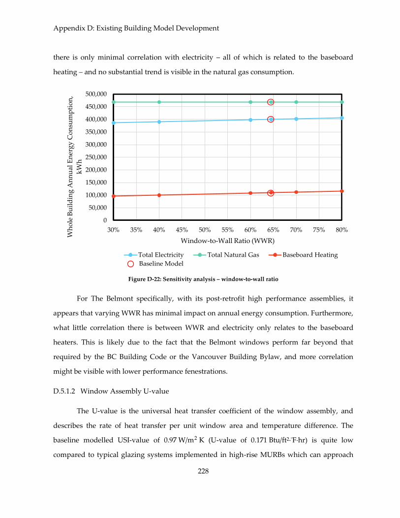
Appendix D: Existing Building Model Development
228
there is only minimal correlation with electricity – all of which is related to the baseboard
heating – and no substantial trend is visible in the natural gas consumption.
Figure D-22: Sensitivity analysis – window-to-wall ratio
For The Belmont specifically, with its post-retrofit high performance assemblies, it
appears that varying WWR has minimal impact on annual energy consumption. Furthermore,
what little correlation there is between WWR and electricity only relates to the baseboard
heaters. This is likely due to the fact that the Belmont windows perform far beyond that
required by the BC Building Code or the Vancouver Building Bylaw, and more correlation
might be visible with lower performance fenestrations.
D.5.1.2 Window Assembly U-value
The U-value is the universal heat transfer coefficient of the window assembly, and
describes the rate of heat transfer per unit window area and temperature difference. The
baseline modelled USI-value of 0.97 W/m2 K (U-value of 0.171 Btu/ft2∙℉∙hr) is quite low
compared to typical glazing systems implemented in high-rise MURBs which can approach
0
50,000
100,000
150,000
200,000
250,000
300,000
350,000
400,000
450,000
500,000
30% 35% 40% 45% 50% 55% 60% 65% 70% 75% 80%
Wh
ole
Bu
ild
ing
An
nu
al E
ner
gy
Co
nsu
mp
tio
n,
kW
h
Window-to-Wall Ratio (WWR)
Total Electricity Total Natural Gas Baseboard Heating
Baseline Model

Appendix D: Existing Building Model Development
229
values as high as 3 W/m2 K in existing buildings. As such, it is necessary to consider the
implications of lower performance windows on the building energy consumption.
Figure D-23 displays the sensitivity analysis conducted on the window U-value with
respect to energy consumption. There is a visible trend between U-value and electricity, but as
with the WWR, this only applies to the baseboard heating.
Figure D-23: Sensitivity analysis – window U-value
The window U-value clearly does correlate with electricity, but as only the baseboard
heating is affected, the overall change in annual energy consumption is still limited. An increase
from the baseline value of USI 0.97 W/m2 K (U-value of 0.171 Btu/ft2∙℉∙hr) to the maximum
value modelled of 1.98 W/m2 K (U-value of 0.35 Btu/ft2∙℉∙hr) increased the baseboard heating
energy by 68%, but this corresponds to an increase in total electricity of 19%, and an increase in
total energy of 9%.
0
50,000
100,000
150,000
200,000
250,000
300,000
350,000
400,000
450,000
500,000
0.85 1.00 1.15 1.30 1.45 1.60 1.75 1.90
Wh
ole
Bu
ild
ing
An
nu
al E
ner
gy
Co
nsu
mp
tio
n,
kW
h
Window USI-value, W/m²-°C
Total Electricity Total Natural Gas Baseboard Heating
Baseline Model

Appendix D: Existing Building Model Development
230
D.5.1.3 Solar Heat Gain Coefficient
The SHGC refers to the percentage of solar energy incident on the window area which
passes through to the interior, and is often discussed at normal incidence although it can be
calculated at any incidence angle. The Belmont windows have an as-built and modelled SHGC
of 0.2, which is very low. Typical values very by window type and manufacturer and are
improving with time. That being said, accepted example values range from 0.45 for triple glazed
windows with low-e coatings to 0.75 for single glazed windows with no coatings (McQuiston
et al., 2005).
Figure D-24 displays the sensitivity analysis conducted on the SHGC, with values
ranging from 0.1 to 0.6. Unlike the previously discussed fenestration properties, the SHGC
shows a negative correlation with energy consumption, which again is tied to the baseboard
heating.
Figure D-24: Sensitivity analysis – solar heat gain coefficient
0
50,000
100,000
150,000
200,000
250,000
300,000
350,000
400,000
450,000
500,000
0.10 0.20 0.30 0.40 0.50 0.60
Wh
ole
Bu
ild
ing
An
nu
al E
ner
gy
Co
nsu
mp
tio
n,
kW
h
Solar Heat Gain Coefficient (SHGC)
Total Electricity Total Natural Gas Baseboard Heating
Baseline Model

Appendix D: Existing Building Model Development
231
The correlation between SHGC and electricity consumption is slight, but definitively
negative. On the surface, this appears contradictory, as higher SHGC values correspond to
cheaper, lower performance windows. However, the decrease in heating electricity is due to
added solar heating, which in turn also increases cooling loads. The Belmont does not have any
active cooling equipment, and therefore the increased solar gains do not appear in the energy
data, but increases are apparent in the temperature and airflow data.
Figure D-25 displays the monthly average operative temperature across all interior
spaces for varying SHGC values. The operative temperature represents the average between
the air and mean radiant temperature within the interior spaces, and is a common metric used
to discuss thermal comfort. ASHRAE Standard 55 provides guidance for thermal comfort,
which is a very complex subject area, but it can generally be observed that while the modelled
temperatures are within acceptable limits, the increasing operative temperature would likely
lead to an increasing number of instances of discomfort among occupants (American Society of
Heating Refrigerating and Air-Conditioning Engineers, 2009). It should also be noted that as
the operative temperature increases with SHGC, so does the disparity between the mean
radiant temperature and the air temperature – a trend that could also lead to thermal comfort
concerns.
Figure D-26 displays a similar trend in increasing air change rates with increasing
SHGC. This is due to the natural ventilation operation scheme implemented in the model which
simulates the opening of windows when the interior temperature exceeds 22°C (72°F).
Combined with the previous plot of operative temperature however it is clear that for SHGC of
0.5 or higher, there are periods when natural ventilation provides inadequate cooling, and some
form of active cooling would likely be required to ensure thermal comfort.

Appendix D: Existing Building Model Development
232
Figure D-25: Sensitivity analysis – solar heat gain coefficient – average monthly operative temperatures
Figure D-26: Sensitivity analysis – solar heat gain coefficient – average monthly air change rates
20.5
21.0
21.5
22.0
22.5
23.0
23.5
24.0
Jan Feb Mar Apr May Jun Jul Aug Sep Oct Nov Dec
Av
erag
e O
per
ativ
e T
emp
erat
ure
, °C
Month
SHGC = 0.1
SHGC = 0.2
SHGC = 0.3
SHGC = 0.4
SHGC = 0.5
SHGC = 0.6
0.00
0.20
0.40
0.60
0.80
1.00
1.20
1.40
1.60
1.80
2.00
Jan Feb Mar Apr May Jun Jul Aug Sep Oct Nov Dec
Wh
ole
Bu
ild
ing
Air
Ch
ang
e R
ate,
1/h
Month
SHGC = 0.1
SHGC = 0.2
SHGC = 0.3
SHGC = 0.4
SHGC = 0.5
SHGC = 0.6

Appendix D: Existing Building Model Development
233
Overall there was a slight negative correlation between energy consumption and
SHGC. Transitioning form the baseline value of 0.2 to the highest value modelled of 0.6, the
baseboard heating decreased by 32% which corresponds to a decreases of 9% in total
electricity and 4% in total energy. While this correlation is modest, it is clear that at higher
SHGC values, thermal comfort would become an issue and some form of cooling would
likely become necessary.
D.5.2 Opaque Wall Insulation
The opaque wall insulation refers to the insulation value of the vertical surfaces not
associated with the fenestrations assemblies on the exterior walls of the building. While the
specific materials used in the wall assembly matter from a building science perspective, in this
case the only relevant parameter is the insulation value which is quantified by the assembly
effective R-value. In the baseline model and as-built building, The Belmont post-retrofit wall
assemblies have an effective RSI-value of 2.82 m2∙K W⁄ (R-value of 16.06 ft2∙℉∙hr/Btu). This
exceeds the BC Building Code and Vancouver Building Bylaw minimum, but is not as
insulating as assemblies used in low energy building construction such as Passive House
(Canadian Passive House Institute, 2016). As such, it is useful is examine effective R-values both
greater than and less than the baseline case.
Figure D-27 displays the sensitivity analysis conducted on the opaque wall RSI-value.
As with the SHGC, a slight negative trend is visible, but this is to be expected based on Fourier’s
Law. Note that within the model, internal areas are calculated based on the perimeter area less
the exterior wall thickness, and so the total wall thickness had to remain constant throughout
all parametric runs in order to avoid inadvertent modification of internal loads which are
applied on a per unit floor area basis. As such, modifications were made to material types and
non-critical material thicknesses, but the thermal mass elements such as the structural concrete
were retained at the baseline values.

Appendix D: Existing Building Model Development
234
Figure D-27: Sensitivity analysis – opaque wall RSI-value
It is clear that while a negative correlation is visible between effective R-value and
energy consumption, it is still fairly minimal. A change from the baseline effective RSI-value of
2.82 m2∙K W⁄ (R-value of 16.06 ft2∙℉∙hr/Btu) to the maximum value modelled of 4.21 m2∙K W⁄ (R-
value of 23.86 ft2∙℉∙hr/Btu) resulted in a decrease of 14% in annual baseboard heating. This
equates to a decrease in total electricity of 4%, and a decrease in total energy of 2%.
D.5.3 Roof Insulation
The roof insulation, as with the opaque wall insulation, is concerned with the effective
R-value of the roof assembly. In the baseline model and as-built construction, The Belmont roof
has an RSI-value of 3.5 m2∙K/W (R-value of 19.9 ft2∙℉∙hr/Btu). Unlike the wall assemblies, the
nature of inverted roof assemblies results in minimal thermal bridging, and therefore the
nominal R-value is usually a valid input when modelling.
Figure D-28 displays the sensitivity analysis conducted on the roof RSI-value. Only a
slight correlation is visible, but as with the wall insulation, the trend is negative.
0
50,000
100,000
150,000
200,000
250,000
300,000
350,000
400,000
450,000
500,000
1.4 1.7 2.0 2.3 2.6 2.9 3.2 3.5 3.8 4.1
Wh
ole
Bu
ild
ing
An
nu
al E
ner
gy
Co
nsu
mp
tio
n,
kW
h
Wall RSI-value, m²-°C/W
Total Electricity Total Natural Gas Baseboard Heating
Baseline Model

Appendix D: Existing Building Model Development
235
Figure D-28: Sensitivity analysis – roof RSI-value
Only a minimal correlation is visible between the roof insulation level and building
energy consumption, with a maximum variation from the baseline electricity consumption of
only ±1% across all values modelled. This minimal variation is likely due to the form factor of
the building, and the fact that only 5 of the 37 suites have any contact with the roof assembly.
D.5.4 Airtightness
Airtightness is a building enclosure performance metric, and describes the amount of
air that can pass through an assembly at a given differential pressure. In application, whole
building airtightness testing is often conducted to in order to quantify the performance of the
air barrier systems. As previously discussed in Section 3.3.2, The Belmont was tested by RDH
and was found to have an overall airtightness of 1.4 Ac/h at 50 Pa.
In the context of energy modelling, air leakage is an important input as it determines
the amount of air exchange simulated across the building enclosure at each time step of the
simulation. Infiltration is distinctly different from airtightness however as infiltration occurs at
0
50,000
100,000
150,000
200,000
250,000
300,000
350,000
400,000
450,000
500,000
1.75 2.75 3.75 4.75 5.75 6.75 7.75 8.75
Wh
ole
Bu
ild
ing
An
nu
al E
ner
gy
Co
nsu
mp
tio
n, k
Wh
Roof R-value, m²-°C/W
Total Electricity Total Natural Gas Baseboard Heating
Baseline Model

Appendix D: Existing Building Model Development
236
much lower differential pressures, and therefore converting between the two represents an
engineering challenge.
In The Belmont model, the infiltration was input in the form of an airtightness value,
and DesignBuilder converted this value to an infiltration rate by means of equation D-1 as
described in BS EN12831 (European committee for Standardization, 2003).
∙ ∙ ∙ ∙ Eq. D-1
where:
While equation D-1 does include a correction factor in an attempt to account for
differences in wind pressure resulting from building height, it makes no attempt to account for
varying building pressures, and therefore represents a fairly simplistic method of converting
airtightness to infiltration.
In the development of the Belmont model, the measured airtightness value of 1.4 Ac/h
at 50 Pa was calibrated to 3.5 Ac/h at 50 Pa in order to get realistic predictions of space heating
loads. This likely indicates that equation D-1 under predicts infiltration, and so more
conservative inputs are required.
Figure D-29 displays the sensitivity analysis conducted on the building enclosure
airtightness value. Note that the airtightness values represent the inputs as entered into
DesignBuilder, and the corresponding real-world airtightness values are likely lower based on
the case of The Belmont specifically.

Appendix D: Existing Building Model Development
237
Figure D-29: Sensitivity analysis – airtightness value as entered into DesignBuilder
It is clear that airtightness is strongly correlated with electricity use, despite the only
end-use associated with the correlation being baseboard heating. A variation from the already
exaggerated value of 3.5 Ac/h at 50 Pa in the baseline model to the maximum value simulated
of 10 Ac/h at 50 Pa resulted in an increase in baseboard heating energy consumption of 182%.
This increase corresponds to an increase in electricity consumption of 42%, and an overall
increase in energy consumption of 19%. From these numbers it is clear that proper input of the
airtightness value is crucial to the accurate simulation of whole building energy consumption,
even in a climate as mild as Vancouver.
D.5.5 Fireplaces
The Belmont has natural gas fireplaces in the living rooms of the suites on the top 5
floors, which corresponds to 13% of the total building annual energy consumption. The
presence of these fireplaces, however, is atypical of new construction high-rise MURBs. As
0
100,000
200,000
300,000
400,000
500,000
600,000
1 2 3 4 5 6 7 8 9 10
Wh
ole
Bu
ild
ing
An
nu
al E
ner
gy
Co
nsu
mp
tio
n,
kW
h
Enclosure Airtightness, Ach-50
Total Electricity Total Natural Gas Baseboard Heating
Baseline Model

Appendix D: Existing Building Model Development
238
such, it is necessary to also consider how the presence of the fireplaces shifts the distribution of
energy consumption between the remaining end-uses.
Figure D-30 displays the annual energy consumption of the major end-uses in The
Belmont model both for the baseline case with fireplaces as well as the alternative case
involving no fireplaces. Aside from the variation in fireplace consumption, removing the
fireplaces increased the baseboard heating energy by 20% or 22,000 kWh/year.
Figure D-30: Sensitivity analysis – The Belmont model with and without fireplaces
Removing the fireplaces results in a decrease of 116,000 kWh of natural gas
consumption, which combined with the increase in electric baseboard consumption of 22,000
kWh leads to a total decrease in consumption of 94,000 kWh. This substantial decrease shifts
the percentage breakdown between the remaining end-uses, which can be seen in Figure D-31.
With the new configuration, the mechanical systems – including the DHW, MAU, baseboard
heaters, system pumps and fans – comprise 65% of the annual energy consumption.
0
20,000
40,000
60,000
80,000
100,000
120,000
140,000
160,000
180,000
200,000
MELs Lighting System
Fans
System
Pumps
Baseboard
Heating
MAU
Heating
DHW Fireplaces
Wh
ole
Bu
ild
ing
An
nu
al E
ner
gy
Co
nsu
mp
tio
n, k
Wh
Baseline Without Fireplaces

Appendix D: Existing Building Model Development
239
Figure D-31: Sensitivity analysis – end-use breakdown of The Belmont model annual consumption without
fireplaces
The change in space heating energy of 22,000 kWh despite the decrease in fireplace
energy of 116,000 kWh indicates that the majority of the energy consumed by the fireplaces was
not effectively contributing to the building space heating needs. This is likely due to the
relatively low efficiency of the fireplaces, which were modelled as having an efficiency of 60%,
all of which acted as radiant heat gains. Additionally, as fireplaces were only present in the
living rooms of the suites on the top 5 floors, they only influenced a small percentage of the
total conditioned floor area. Overall, the fireplaces consumed a large percentage of the total
building energy use despite not contributing significantly to the space heating loads.
D.5.6 Enclosed Balconies
In addition to the fireplaces, another atypical building characteristic of The Belmont is
the presence of enclosed balconies. These zones represent spaces within the outer building
enclosure that are additionally separated from conditioned interior space, and have no active
conditioning equipment installed.
Within the energy model of the Belmont, the enclosed balconies were modified in order
to treat the zones differently. The easiest change to implement involved simply changing the
MELs, 153,228 ,
20%
Lighting, 115,738
, 15%
System Fans,
18,601 , 2%
System Pumps,
2,177 , 0%Baseboard
Heating, 131,812 ,
17%
MAU Heating,
186,568 , 24%
DHW, 168,425 ,
22%

Appendix D: Existing Building Model Development
240
designation of these spaces such that they were also conditioned with baseboard electric
heating in order to be consistent with the rest of the suite conditioned floor area. This addition
of 316 m2 (3,400 ft2) of conditioned floor area caused an increase in baseboard electricity
consumption of 11% annually. While not a substantial change in this end-use, the additional
energy does change the end-use splits as depicted in Figure D-32.
Figure D-32: Sensitivity analysis – end-use breakdown of The Belmont model annual consumption without
enclosed balconies
Modifying the model to include the enclosed balconies as conditioned interior space did
increase the space heating load slightly, but had a minimal increase on overall energy
consumption of 1%. A slight improvement was also visible in the mean operative temperature
during winter months. Overall the change had minimal impact on the whole building
consumption values.
D.5.7 Location
The building location determines the loads experienced by the space conditioning
systems, and by extension has a large influence over the whole building energy use.
Construction practices and system selections can be regionally specific for a wide variety of
reasons, include local building codes and material availability. Furthermore, it would be
MELs, 153,228 ,
18%
Lighting, 115,738
, 13%
System Fans,
18,601 , 2%
System Pumps,
2,177 , 0%
Baseboard
Heating, 122,149 ,
14%
MAU Heating,
186,568 , 21%
DHW, 166,240 ,
19%
Fireplaces,
115,734 , 13%

Appendix D: Existing Building Model Development
241
unlikely for a building with all of The Belmont’s characteristics to be constructed in a colder
climate zone than Vancouver, but it is useful to evaluate the impact varying climate types
would have on the annual energy use.
Figure D-33 displays the end-use energy consumption of the Belmont for a variety of
different weather files. Note that the baseline used the Vancouver International Airport 2013
actual meteorological year (AMY), while the other weather files are based on typical
meteorological year (TMY) data from the CWEC database.
Figure D-33: Sensitivity analysis – location
The only end-uses correlated with location are baseboard heating and MAU heating,
but the variation from Vancouver to Edmonton was substantial; baseboard heating energy
increased by 126%, and make-up air heating energy increased by 70%. Figure D-34 displays the
end-use consumption splits based on the Edmonton typical meteorological year weather file.
The increase in space conditioning loads in Edmonton results in a shift in end-use
consumption such that HVAC and DHW systems now constitute 67% of the total annual energy
consumption as opposed to 55% in the baseline scenario. While the specific systems and
equipment may be different based on typical practices under the Alberta Building Code, it is
0
50,000
100,000
150,000
200,000
250,000
300,000
350,000
MELs Lighting System
Fans
System
Pumps
Baseboard
Heating
MAU
Heating
DHW Fireplaces
Wh
ole
Bu
ild
ing
An
nu
al E
ner
gy
Co
nsu
mp
tio
n, k
Wh
Baseline Vancouver TMY Toronto TMY Edmenton TMY
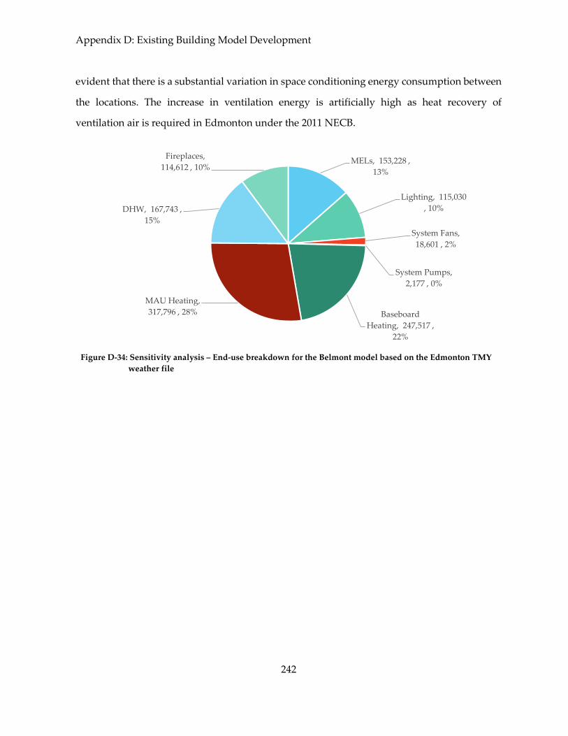
Appendix D: Existing Building Model Development
242
evident that there is a substantial variation in space conditioning energy consumption between
the locations. The increase in ventilation energy is artificially high as heat recovery of
ventilation air is required in Edmonton under the 2011 NECB.
Figure D-34: Sensitivity analysis – End-use breakdown for the Belmont model based on the Edmonton TMY
weather file
MELs, 153,228 ,
13%
Lighting, 115,030
, 10%
System Fans,
18,601 , 2%
System Pumps,
2,177 , 0%
Baseboard
Heating, 247,517 ,
22%
MAU Heating,
317,796 , 28%
DHW, 167,743 ,
15%
Fireplaces,
114,612 , 10%

Appendix E: Mechanical System Model Inputs
243
Appendix E: Mechanical System Model Inputs
In this section, the modelling inputs required to configure each of the independent
mechanical systems identified in the main body of the thesis are listed. Figure E-1 displays the
different system type numbers, as discussed in Chapter 2. Table E-1 summarizes the different
system types as classified for this analysis. Table E-2 provides relevant information and
explanations of acronyms and abbreviations used throughout this appendix. Table E-3
describes each system, with subsequent tables denoting the specific modelling inputs
associated with each system.
1. Thermal Comfort Systems
2. Indoor Air Quality Systems
3. Domestic Hot Water Systems
Heating Cooling Humidity Control Airflow Control (Velocity)
Ventilation Filtration Airflow Control (Pressure)
Domestic Hot Water
Figure E-1: Residential mechanical system types 1-3 as defined for the purposes of this body of work. This
figure is repeated from Section 2.5 for convenience

Appendix E: Mechanical System Model Inputs
244
Table E-1: Residential mechanical system types – as classified based on their primary functions served
System
Type
Primary Functions
Served Notes
1a Heating May also provide filtration, humidity, airflow control
1b Cooling May also provide filtration, humidity, airflow control
1c Heating
Cooling May also provide filtration, humidity, airflow control
2a Suite Ventilation May also provide filtration, humidity, airflow control
2b Corridor Ventilation May also provide filtration, humidity, airflow control
2c Suite Ventilation
Corridor Ventilation May also provide filtration, humidity, airflow control
3 Domestic Hot Water
Table E-2: Acronyms and abbreviations used throughout this appendix
Term Meaning Description
S/S Suite by suite layout
Refers to systems which have all energy
production/rejection components located within
individual suites
F/F Floor by floor layout
Refers to systems which have all energy
production/rejection components located on each
floor in common space
C/ Centralized
Refers to systems which have all energy
production/rejection components located in one
central area of the building
V Vancouver Used to abbreviate location modelled
T Toronto Used to abbreviate location modelled
E Edmonton Used to abbreviate location modelled

Appendix E: Mechanical System Model Inputs
245
Table E-3: Mechanical system descriptions
System
Number
System
Type
Primary
Fuel Layout
Distribution
Medium Description
Locations
Modelled
1 1a Elec S/S N/A Electric resistance, convective heating V, T, E
2 1a Elec S/S Air In-suite AHU with forced air electric furnace V, E
3 1a Gas S/S Air In-suite AHU with forced air natural gas furnace V, E
4 1a Gas C/ Water Radiant floor with centralized natural gas boiler V, T, E
5 1a Gas C/ Water 2-pipe FCUs with centralized natural gas boiler V, E
6 1a Gas C/ Water Hydronic convectors with central natural gas boiler V, T, E
7 1b Elec S/S N/A PTAC, no heating T
8 1b Elec C/ Water Chilled ceilings with central chiller, cooling tower T
9 1c Elec S/S N/A PTAC, electric heating coil V, T, E
10 1c Elec S/S N/A PTHP, electric backup heating coil V, T, E
11 1c Elec S/S Air In-suite AHU, electric furnace, dx cooling T
12 1c Elec/Gas S/S Air In-suite AHU, natural gas furnace, dx cooling T
13 1c Elec S/S Refrigerant Central VRF system, air source heat pump V, T, E
14 1c Elec S/S Refrigerant Central VRF system, ground source heat pump V, T, E
15 1c Elec/Gas C/ Water 4-pipe FCUs, central natural gas boiler, chiller, cooling tower T
16 1c Elec/Gas C/ Air/Water In-suite WSHP, central natural gas boiler, cooling tower T
17 2a Elec S/S Air In-suite Heat Recovery Ventilator (HRV) V, T, E

Appendix E: Mechanical System Model Inputs
246
System
Number
System
Type
Primary
Fuel Layout
Distribution
Medium Description
Locations
Modelled
18 2a Elec S/S Air In-suite Energy Recovery Ventilator (ERV) V, T, E
19 2b Elec F/F Air Floor AHU, DOAS serving corridors, heat recovery V, T, E
20 2b Elec F/F Air Floor AHU, DOAS serving corridors, enthalpy recovery V, T, E
21 2b Elec C/ Air Central AHU, DOAS serving corridors, heat recovery V, T, E
22 2b Elec C/ Air Central AHU, DOAS serving corridors, enthalpy recovery V, T, E
23 2c Elec F/F Air Floor AHU, DOAS serving suites + corridors, heat recovery V, T, E
24 2c Elec F/F Air Floor AHU, DOAS serving suites + corridors, enthalpy recovery V, T, E
25 2c Elec C/ Air Central AHU, DOAS serving suites + corridors, heat recovery V, T, E
26 2c Elec C/ Air Central AHU, DOAS serving suites + corridors, enthalpy recovery V, T, E
27 2c Elec/Gas C/ Air Central MAU, corridor pressurization, natural gas heat V, T, E
28 3 Elec S/S Water In-suite electric storage tank water heater V, T, E
29 3 Gas S/S Water In-suite natural gas storage tank water heater V, T, E
30 3 Elec S/S Water In-suite electric tankless water heater V, T, E
31 3 Gas S/S Water In-suite natural gas tankless water heater V, T, E
32 3 Elec F/F Water Floor electric storage tank water heater V, T, E
33 3 Gas F/F Water Floor natural gas storage tank water heater V, T, E
34 3 Elec C/ Water Central electric boiler with storage tanks V, T, E
35 3 Gas C/ Water Central natural gas boiler with storage tanks V, T, E

Appendix E: Mechanical System Model Inputs
247
System
Number
System
Type
Primary
Fuel Layout
Distribution
Medium Description
Locations
Modelled
36 3 Elec C/ Water Central solar thermal hot water system, electric boiler V, T, E
37 3 Gas C/ Water Central solar thermal hot water system, natural gas boiler V, T, E
38 1a+2a Elec S/S Air In-suite AHU w/ OA heat recovery, electric furnace V, E
39 1a+2a Gas S/S Air In-suite AHU w/ OA heat recovery, natural gas furnace V, E
40 1a+2a Elec S/S Air In-suite AHU w/ OA enthalpy recovery, electric furnace V, E
41 1a+2a Gas S/S Air In-suite AHU w/ OA enthalpy recovery, natural gas furnace V, E
42 1a+2a Gas C/ Water 2-pipe FCUs w/ OA intake, centralized natural gas boiler V, E
43 1c+2a Elec S/S N/A PTAC, electric heating coil, OA intake, point exhaust V, T, E
44 1c+2a Elec S/S N/A PTHP, OA intake, point exhaust V, T, E
45 1c+2a Elec S/S Air In-suite AHU w/ OA heat recovery, electric furnace, dx cooling T
46 1c+2a Elec/Gas S/S Air In-suite AHU w/ OA heat recovery, natural gas furnace, dx cooling T
47 1c+2a Elec S/S Air In-suite AHU w/ OA enthalpy recovery, electric furnace, dx cooling T
48 1c+2a Elec/Gas S/S Air In-suite AHU w/ OA enthalpy recovery, natural gas furnace, dx
cooling T
49 1c+2a Elec/Gas C/ Water 4-pipe FCUs w/ OA intake, central natural gas boiler, chiller, cooling
tower T
50 1c+2a Elec/Gas C/ Air/Water In-suite WSHP w/OA enthalpy recovery, central natural gas boiler,
cooling tower T

Appendix E: Mechanical System Model Inputs
248
System
Number
System
Type
Primary
Fuel Layout
Distribution
Medium Description
Locations
Modelled
51 1c+2a Elec/Gas C/ Air/Water In-suite WSHP w/ OA heat recovery, central natural gas boiler,
cooling tower T
52 1a+3 Gas S/S Water Radiant floor, in-suite gas tank water heater V, E
53 1a+3 Gas S/S Water Hydronic convectors, in-suite gas tank water heater V, E
54 1a+3 Gas S/S Air/Water In-suite AHU w/ HW coil, in-suite gas tank water heater V, E
55 1a+3 Gas S/S Air/Water In-suite AHU w/ HW coil, in-suite gas tankless water heater V, E
56 1a+3 Gas C/ Water Radiant floor, central gas boiler, providing DHW V, E
57 1a+3 Gas C/ Water 2-pipe FCUs, central gas boiler, providing DHW V, E
58 1a+3 Gas C/ Air/Water In-suite AHU w/ HW coil, central gas boiler, providing DHW V, E
59 1a+3 Gas C/ Water Hydronic convectors, central gas boiler, providing DHW V, E
60 1c+3 Elec/Gas S/S Air/Water In-suite Ducted FCU, dx cooling, in-suite natural gas storage tank
water heater T
61 1c+3 Elec/Gas S/S Air/Water In-suite Ducted FCU, dx cooling, in-suite natural gas tankless water
heater T
62 1c+3 Elec/Gas C/ Water 4-pipe FCUs, central natural gas boiler with storage tanks, chiller,
cooling tower, providing DHW T
63 1c+3 Elec/Gas C/ Air/Water In-suite WSHP, central natural gas boiler with storage tanks, cooling
tower, providing DHW T

Appendix E: Mechanical System Model Inputs
249
Table E-4: Modelling inputs – energy production/rejection components
Equipment Model Inputs
Condensing Gas Boiler
90% full load thermal efficiency (higher values result in
part load/ low return temp efficiencies >100%)
DesignBuilder default condensing boiler part load curves
25 W parasitic exhaust fan load as DesignBuilder default
25 ft H2O pump head, 90% full load efficiency with variable
flow, intermittent control except for radiant floors
Boiler LWTs depend on system.
Design supply/return delta of 10-15°C
Non-Condensing Gas
Boiler
This only applies to hydronic systems with high water
temperatures, such as hydronic convectors
82% full load thermal efficiency (Charbonneau, 2011)
DesignBuilder default non-condensing boiler part load
curves
25 W parasitic exhaust fan load as DesignBuilder default
25 ft H2O pump head, 90% full load efficiency with variable
flow, intermittent control except for radiant floors
Boiler LWTs depend on system.
Design supply/return delta of 10°C
Chiller
Water cooled reciprocating chiller
COP of 5.0, about 0.7 kW/Ton (Natural Resources Canada,
2002)
DOE-2 Reciprocating chiller part load curves
Default DesignBuilder reference temperatures
25 ft H2O pump head, 90% full load efficiency with variable
flow, intermittent control except for chilled ceilings
Design LWTs depend on system
Design supply/return delta of 4°C
Cooling Tower
Single speed, fan cycling
Blowdown concentration ratio of 3.0
Condenser loop temperature set to follow outdoor air dry
bulb temperature, min/max of 10°C/50°C
Ground Exchange Loop
Ground temperature of 13°C (56°F) from DesignBuilder
default
Vertical U-tube borehole field, 76m (250 ft) deep, 240
boreholes
Borehole properties left at DesignBuilder defaults: 2.5”
borehole radius, 1” pipe outer diameter, 1” U-tube distance
Default G-function data for ground exchange calculations
Supply water temperature set to follow ground
temperature

Appendix E: Mechanical System Model Inputs
250
Equipment Model Inputs
Central MAU
Gas heating coil efficiency of 90%
DX cooling SEER of 11
Supply ductwork only
Supply fan static pressure of 1” H2O, fan efficiency of 45%,
motor efficiency of 90%
Delivery effectiveness of 1.0
Central AHU
Gas heating coil efficiency of 95% (if heating included)
DX cooling SEER of 17 (if cooling included)
Supply and return ductwork
Heat recovery/ enthalpy recovery as below
Supply fan static pressure of 1” H2O + 0.5” for heat
recovery, 0.5” if ducted to suites
Fan efficiency of 45%, motor efficiency of 90%
Delivery effectiveness of 1.0 to corridors, 0.8 to suites
In-suite AHU
95% gas furnace thermal efficiency, fully modulating,
variable capacity (Charbonneau, 2011)
DX cooling SEER of 17 (Natural Resources Canada, 2015)
Fan static pressure of 0.5” H2O + 0.5” for heat recover, 45%
fan efficiency, 70% motor efficiency (Canadian Mortgage
and Housing Corporation, 2015; Kohta Ueno, 2010b)
Delivery effectiveness of 0.8 if supplying outdoor air
HRV/ ERV
Sensible effectiveness: 0.8 at 75% heating flow, 0.8 at 75%
cooling flow, 0.7 at 100 % heating flow, 0.7 at 100% cooling
flow
Delivery effectiveness of 0.5 without ductwork, 0.8 with
ductwork delivering hot air at high level
Defrost strategy for floor/central systems involves electric
preheat coil with 5°C setpoint, only necessary in Edmonton
HRVs use a plate heat exchanger, ERVs use a rotary wheel
Storage Tank Domestic
Hot Water Heaters
Gas water heater energy factor of 0.7 (Natural Resources
Canada, 2012)
10% improvement on energy factor if providing space
heating, resulting in an energy factor of 0.8 (Clinton, 1999)
In-suite pumps with 1/3 hp motor, 5 ft H2O head, 70%
motor efficiency
Instantaneous Domestic
Hot Water Heaters
Gas instantaneous water heater energy factor of 0.98
(Natural Resources Canada, 2012)
Internal storage of 1 US gallon
In-suite pumps with 1/3 hp motor, 70% motor efficiency

Appendix E: Mechanical System Model Inputs
251
Equipment Model Inputs
Solar Thermal Domestic
Hot Water Heater
Veissman SV1 flat plate collector selected as solar thermal
array from 86 pre-loaded templates found in DesignBuilder
based on previous experience with this collector
Collector array located on the southern side of the roof,
facing south at a 45° angle
Each collector is 27 ft2 of total area, with a total of 12
collectors (this is the maximum number that can be
connected to one loop according to the manufacturer)
Approximately one collector per floor
One solar loop storage tank
Backup heating provided by electric or natural gas boiler
connected to storage tanks. See condensing natural gas
boiler for assumptions
Solar loop and hot water loop pumps selected as 1/3 hp
with 10 ft H2O head and a motor efficiency of 90%
VRF Outdoor Unit
VRF outdoor units are defined by 26 part load curves in
DesignBuilder
Accurate modelling of a general case system is difficult.
Used LG VRF predefined systems, up to 36 tons’ capacity
per system depending on building demand
Natural ventilation interior maximum temperature setpoint
of 75.5°F
For Edmonton, minimum compressor operation
temperature lowered from -25°C to -35°C
Table E-5: Modelling inputs – Terminal Units
Equipment Model Inputs
Electric Baseboards Zone equipment: electric convectors
Hydronic Baseboards
Zone equipment: water convector
Supply water temperature of 70°C from boiler loop, 10°C
loop delta T

Appendix E: Mechanical System Model Inputs
252
Equipment Model Inputs
Fan Coil Units
Zone equipment: 4-pipe FCU (no option for 2-pipe, so
chilled water loop included but not enabled for heating
only systems)
Supply water temperature of 65°C from boiler loop, 15°C
loop delta T
Fan static pressure of 0.5” H2O, 45% fan efficiency, 70%
motor efficiency (Canadian Mortgage and Housing
Corporation, 2007; Kohta Ueno, 2010b)
When cooling provided, natural ventilation interior
maximum temperature setpoint of 75.5°F
Radiant Floors
Zone Equipment: heated floor
Internal floor construction consisting of 6” concrete, 1” EPS,
1.5” cement screed, 0.3” ceramic tile
Internal source (hydronic piping) placed above EPS layer,
with 2D option enabled and at a spacing of 8”
Interior heating setpoint changed to 70.5°F code, 71.5°F
low-energy, with operative temperature control instead of
air temperature control
Supply water temperature varied from 30 to 50°C based on
outdoor air reset between -8 and 22°C
Chilled Ceilings
Zone Equipment: chilled ceiling
Internal ceiling construction consisting of the reverse of the
that used for radiant floors (6” concrete, 1” EPS, 1.5”
cement screed, 0.3” ceramic tile)
Internal source (hydronic piping) placed below EPS layer,
with 2D option enabled and at a spacing of 8”
Operative temperature control instead of air temperature
control
Supply water temperature of 13°C
Packaged Terminal Air
Conditioner (PTAC)
Zone equipment: PTAC
Heating provided by electric resistance coil, COP=1
Target SEER-17 (COP-5.0) (Natural Resources Canada,
2015)
Fan static pressure of 0.5” H2O, 45% fan efficiency, 70%
motor efficiency (Canadian Mortgage and Housing
Corporation, 2007; Kohta Ueno, 2010b)
Natural ventilation interior maximum temperature setpoint
of 75.5°F
VRF Indoor Units Zone equipment: VRF indoor unit

Appendix E: Mechanical System Model Inputs
253
Equipment Model Inputs
Vertical Stacked Water
Source Heat Pump
(WSHP)
Zone equipment: water-to-air heat pump
Heating COP of 5, cooling COP of 4.4 (Daikin Applied,
2015; Trane, 2015)
Part load performance left at DesignBuilder default based
on equation fit method
Fan controlled by cycling, static pressure of 0.5” H2O, 45%
fan efficiency, 70% motor efficiency (Canadian Mortgage
and Housing Corporation, 2007; Kohta Ueno, 2010b)
Natural ventilation interior maximum temperature setpoint
of 75.5°F
Packaged Terminal Heat
Pump (PTHP)
Zone equipment: PTHP
Backup heating provided by electric resistance coil, COP=1
Target HSPF-8.6 (COP-2.5), SEER-17 (COP-5.0) (Natural
Resources Canada, 2015)
Minimum temperature for compressor = -10°C
Maximum temperature for resistance heating = 21°C
Defrost strategy: reverse cycle, max temperature of 5°C for
running defrost cycle
Fan static pressure of 0.5” H2O, 45% fan efficiency, 70%
motor efficiency (Canadian Mortgage and Housing
Corporation, 2007; Kohta Ueno, 2010b)
Natural ventilation interior maximum temperature setpoint
of 75.5°F

Appendix F: Emission Factors and Utility Prices
254
Appendix F: Emission Factors and Utility Prices
In order to convert the energy consumption data generated through building simulation
to annual greenhouse gas emissions and operating costs, conversion factors are necessary. Table
F-1 displays the conversion factors used to generate the results presented in Chapter 4.
Table F-1: Greenhouse gas emission factors and blended average energy costs for conversion between energy
consumption and GHG emissions, operating costs (BC Ministry of Environment, 2014; Canadian
Mortgage and Housing Corporation, 2015)
Location Utility
Emission Factor
Kg eCO2 per kWh
(Kg eCO2 per GJ)
Energy Cost
CAD per kWh
(CAD per m3)
Vancouver
Electricity 0.0101
(2.8)
$0.116
Natural Gas 0.1791
(49.75)
$0.0322
($0.34)
Toronto
Electricity 0.1044
(29)
$0.12
Natural Gas 0.1791
(49.75)
$0.0265
($0.28)
Edmonton
Electricity 0.8100
(225)
$0.11
Natural Gas 0.1791
(49.75)
$0.0104
($0.11)