a study on neural network based system identification...

A STUDY ON NEURAL NETWORK BASED SYSTEM IDENTIFICATION WITH APPLICATION TO HEATING,

VENTILATING AND AIR CONDITIONING (HVAC) SYSTEM

A THESIS SUBMITTED IN PARTIAL FULFILLMENT

OF THE REQUIREMENTS FOR THE DEGREE OF

Master of Technology

In

ELECTRONIC SYSTEMS AND COMMUNICATIONS

By

SATH YAM BONALA

ROLL. NO: 207EE107

----------------------------------------------------------------------------------------------------------------

Department of Electrical Engineering

National Institute of Technology, Rourkela

May, 2009

A STUDY ON NEURAL NETWORK BASED SYSTEM IDENTIFICATION WITH APPLICATION TO HEATING,

VENTILATING AND AIR CONDITIONING (HVAC) SYSTEM

A THESIS SUBMITTED IN PARTIAL FULFILLMENT

OF THE REQUIREMENTS FOR THE DEGREE OF

Master of Technology

In

ELECTRONIC SYSTEMS AND COMMUNICATIONS

By

SATHYAM BONALA

ROLL. NO: 207EE107

Under the Guidance of

Prof. Bidyadhar Subudhi

----------------------------------------------------------------------------------------------------------------

Department of Electrical Engineering

National Institute of Technology, Rourkela

May, 2009

National Institute Of Technology

Rourkela-769008, Orissa

CERTIFICATE

This is to certify that the thesis entitled, ―A STUDY ON NEURAL NETWORK BASED

SYSTEM IDENTIFICATION WITH APPLICATION TO HEATING, VENTILATING

AND AIR-CONDITIONING (HVAC) SYSTEM” submitted by Mr. SATHYAM

BONALA in partial fulfillment of the requirements for the award of Master of Technology

Degree in Electrical Engineering with specialization in “ELECTRONIC SYSTEMS AND

COMMUNICATIONS” at the National Institute of Technology, Rourkela is an authentic

work carried out by him under my supervision and guidance.

To the best of my knowledge, the matter embodied in the thesis has not been submitted to any

other University / Institute for the award of any Degree or Diploma.

Date: PROF. BIDYADHAR SUBUDHI

SUPERVISOR

ACKNOWLEDGEMENTS

This project is by far the most significant accomplishment in my life and it would be

impossible without people who supported me and believed in me.

I would like to extend my gratitude and my sincere thanks to my honorable, esteemed

supervisor Prof. Bidyadhar Subudhi, Head, Department of Electrical Engineering. He is not

only a great lecturer with deep vision but also most importantly a kind person. I sincerely

thank for his exemplary guidance and encouragement. His trust and support inspired me in

the most important moments of making right decisions and I am glad to work under his

supervision.

I want to thank all my teachers Prof. J.K. Satapathy, Prof. S. Das, Prof. D. Patra,

Mrs. K.R. Subhashini, Mr. S. Mohanthy and Mr. Debashish Jena for providing a solid

background for my studies. They have been great sources of inspiration to me and I thank

them from the bottom of my heart.

I would like to thank all my friends and especially my classmates for all the

thoughtful and mind stimulating discussions we had, which prompted us to think beyond the

obvious. I’ve enjoyed their companionship so much during my stay at NIT, Rourkela.

I would like to thank all those who made my stay in Rourkela an unforgettable and

rewarding experience.

Last but not least I would like to thank my parents, who taught me the value of hard

work by their own example. They rendered me enormous support being apart during the

whole tenure of my stay in NIT Rourkela.

SATHYAM BONALA

CONTENTS Page No.

Abstract i

List of Figures ii

Abbreviations iii

Chapter 1 Introduction 1

1.1. Introduction 2

1.2. Background study 3

1.3. Motivation 8

1.4. Literature Review 9

1.5. Problem Formulation 10

1.6. Implementation Approaches 11

1.7. Contribution of the Thesis 11

1.8. Thesis Layout 11

Chapter 2 HVAC System Model 13

2.1. Introduction 14

2.2. Working of an HVAC System 14

2.3. HVAC system model 16

2.4. Simulation Results 18

2.5. Heating and cooling. 20

2.6. Heating system. 24

2.7. Ventilating system. 24

2.8. Air conditioning system 25

Chapter 3 System Identification Using Artificial Neural Networks 27


3.2. Neuron Structure 29

3.3. Multilayer Perceptron 32


3.5. Functional Link ANN 37


Chapter 4 Modified Back propagation and Back propagation algorithms 42


4.2. Emotional Back propagation Learning Algorithm. 46

4.2.1 Input-layer neurons. 46

4.2.2 Hidden-layer neurons. 46

4.2.3 Output-layer neurons. 48

4.2.4 The emotional Back propagation parameters 49

4.3. Back propagation weight updation Rule. 51


4.5. Comparison of Results 59

4.6. Performance of different techniques 60

Chapter 5 Adaptive Neuro-fuzzy inference system 61

5.1 Introduction 62

5.2. Fuzzy If-Then Rules and Fuzzy Inference Systems 62

5.3. ANFIS: Adaptive Network-Based Fuzzy-inference System 65

5.4. ANFIS Learning Algorithm 70


Chapter 6 Conclusions and Suggestions for future work 73

6.1 Conclusions 74

6.2 Suggestions for Future Work 74

References 75

i

ABSTRACT

Recent efforts to incorporate aspects of artificial intelligence into the design and operation of

automatic control systems have focused attention on techniques such as fuzzy logic, artificial

neural networks, and expert systems. Although LMS algorithm has been considered to be a

popular method of system identification but it has been seen in many situations that accurate

system identification is not achieved by employing this technique. On the other hand,

artificial neural network (ANN) has been chosen as a suitable alternative approach to

nonlinear system identification due to its good function approximation capabilities i.e. ANNs

are capable of generating complex mapping between input and output spaces. Thus, ANNs

can be employed for modeling of complex dynamical systems with reasonable degree of

accuracy.

The use of computers for direct digital control highlights the recent trend toward more

effective and efficient heating, ventilating, and air-conditioning (HVAC) control

methodologies. The HVAC field has stressed the importance of self learning in building

control systems and has encouraged further studies in the integration of optimal control and

other advanced techniques into the formulation of such systems. In this thesis we describe the

functional link artificial neural network (FLANN), Multi-Layer Perceptron (MLP) with

Back propagation (BP) and MLP with modified BP called the emotional BP and Neuro

fuzzy approaches for the HVAC System Identification.

The thesis describes different architectures together with learning algorithms to build

neural network based nonlinear system identification schemes such as Multi-Layer

Perceptron (MLP) neural network, Functional Link Artificial Neural Network (FLANN) and

ANFIS structures. In the case of MLP used as an identifier, different structures with regard to

hidden layer selection and nodes in each layer have been considered. It may be noted that

difficulty lies in choosing the number of hidden layers for achieving a correct topology of

MLP neural identifier. To overcome this, in the FLANN identifier hidden layers are not

required whereas the input is expanded by using trigonometric polynomials i.e. with cos(nπu)

and sin(nπu), for n=0,1,2,…. The above ANN structures MLP, FLANN and Neuro-fuzzy

(ANFIS Model) have been extensively studied.

ii

LIST OF FIGURES

Figure No. Page No.

1.1 Block Diagram of System Identification 4

1.2 Type of adaptations 6

1.3 Direct Modeling 6

1.4 Inverse Modeling 8

1.5 Implementation of System Identification Technique 10

2.1 Air flow diagram 15

2.2 HVAC System model 16

3.1 Neuron Structure 29

3.2 Structure of Multilayer Perceptron 32

3.3 Neural Network with Back Propagation Algorithm 33

3.8 Structure of FLANN 38

4.1 Input/output configuration of input layer neuron 45

4.2 Input/output configuration of hidden layer neuron 46

4.3 Input/output configuration of output layer neuron 48

4.4 Multilayer perceptron 51

4.5 Notation for back propagation rule 52

5.1 Fuzzy inference system 62

5.2 Fuzzy if-then rules and fuzzy reasoning mechanisms 64

5.3 (a) Type-3 fuzzy reasoning 66

5.3(b) Type-3 ANFIS (Basic structure of ANFIS) 66

5.4(a) Type-1 fuzzy reasoning 67

5.4 (b) Type-1 ANFIS 68

5.5(a) 2 Input type-3 ANFIS with 9 rules 69

5.5(b) Fuzzy Subspaces 69

iii

ABBREVIATIONS USED

ANN Artificial Neural Network

MLP Multilayer Perceptron

FLANN Functional Link Artificial Neural

Network

BP Back Propagation

FIR Finite Impulse Response

IIR Infinite Impulse Response

MSE Mean Square error

HVAC Heating ventilating and Air conditioning

IAQ Indoor air quality

ICU Intensive air uit

CFM Cubic feet for minute

BPA Back propagation algorithm

EmBP Emotional Back propagation

RTU Roof top unit

CER Clean Environment Rooms

ISI Inter Symbol Interference

VOC Volatile organic compounds

ANFIS Adaptive Neuro-fuzzy inference system

CHAPTER 1

INTRODUCTION

2

1.1 INTRODUCTION System Identification is an essential requirement in areas such as control, communication,

power system and instrumentation for obtaining a model of a system (plant) of interest or a

new system to be developed. For the purpose of development of control law, analysis fault

diagnosis, etc.

Major advances have been made in adaptive identification and control, in past few

decades for identifying linear time-invariant plants with unknown parameters. The choice of

the identifier structure is based on well established results in linear systems theory. Stable

adaptive laws for the adjustment of parameters in these which assures the global stability of

the relevant overall systems are also based on properties of linear systems as well as stability

results that are well known for such systems [1]. In this thesis, the major interest is in the

identification of nonlinear dynamic systems using Neural Networks.

The climatisation of rooms in buildings can be quite a complex control problem if

high degrees of comfort and energy saving are required. There are many factors influencing

an environment: humidity, outdoor temperature, solar radiation, neighbouring rooms, people

presence, furniture in the room, heat sources (as computers), windows, heaters, coolers etc.

All these factors have a complex interaction with the comfort and the energy demand.

From the automation point of view, the objective of modeling a building is not to

precisely calculate the temperature in every point of a room, but to have information that can

lead to a successful controller design. This means that the distributed, continuous, and

eventually non-linear process should, with sufficient precision, be described by a lumped LTI

parameters model. If the room is architecturally well designed and the actuators well placed,

comfort and energy-saving can be obtained.

A predictive HVAC controller can potentially obtain the best compromise between

comfort and energy saving. The scheduled room occupation can be prepared with the just

needed in-advance acclimatization, a quite unique characteristic of predictive controllers.

The nonlinear functional mapping properties of neural networks are central to their

use in identification and control. Although a number of key theoretical problems remain,

results pertaining to the approximation capabilities of neural networks demonstrate that they

have great promise in the modeling of nonlinear systems. An important question in system

identification is whether a system under study can be adequately represented within a given

model structure. In the absence of such concrete theoretical results for neural networks, it is

3

usually assumed that the system under consideration belongs to the class of systems that the

chosen network is able to represent.

1.2 BACKGROUND STUDY

The area of system identification is one of the most important areas in engineering because

most of the dynamical system behavior can be obtained exploiting system identification

techniques. For identifying an unknown dynamic systems two things are important i.e. model

structure and then parameters.

Adaptive Modeling and System Identification are prerequisite before going to design a

controller for an on-line plant, say for a scenario an on-line plant requires a controller for

improving its performance. The controller cannot be operated on the on-line plant as it may

disturb the entire production which may be cost effective, so a model is required which

represents the on-line plant. Here comes the concept of modeling a plant. If there is

Adaptability in modeling there is more chance of controlling the model on-line thus Adaptive

modeling of a plant is done.

System identification concerns with the determination of a system, on the basis of input

output data samples. The identification task is to determine a suitable estimate of finite

dimensional parameters which completely characterize the plant. The selection of the

estimate is based on comparison between the actual output sample and a predicted value on

the basis of input data up to that instant. An adaptive automaton is a system whose structure

is alterable or adjustable in such a way that its behavior or performance improves through

contact with its environment. Depending upon input-output relation, the identification of

systems can have two groups

A. Static System Identification

In this type of identification the output at any instant depends upon the input at that instant.

These systems are described by the algebraic equations. The system is essentially a memory

less one and mathematically it is represented as y(n) = f [x(n)] where y(n) is the output at the

nth

instant corresponding to the input x(n).

B. Dynamic System Identification

In this type of identification the output at any instant depends upon the input at that instant as

well as the past inputs and outputs. Dynamic systems are described by the difference or

4

differential equations. These systems have memory to store past values and mathematically

represented as y(n)=f [x(n), x(n-1),x(n-2)………..y(n-1),y(n-2),……] where y(n) is the output at

the nth

instant corresponding to the input x(n).

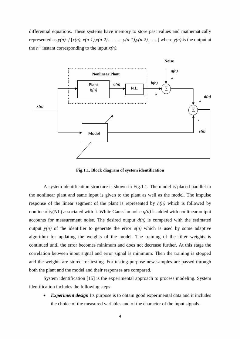
Fig.1.1. Block diagram of system identification

A system identification structure is shown in Fig.1.1. The model is placed parallel to

the nonlinear plant and same input is given to the plant as well as the model. The impulse

response of the linear segment of the plant is represented by h(n) which is followed by

nonlinearity(NL) associated with it. White Gaussian noise q(n) is added with nonlinear output

accounts for measurement noise. The desired output d(n) is compared with the estimated

output y(n) of the identifier to generate the error e(n) which is used by some adaptive

algorithm for updating the weights of the model. The training of the filter weights is

continued until the error becomes minimum and does not decrease further. At this stage the

correlation between input signal and error signal is minimum. Then the training is stopped

and the weights are stored for testing. For testing purpose new samples are passed through

both the plant and the model and their responses are compared.

System identification [15] is the experimental approach to process modeling. System

identification includes the following steps

Experiment design Its purpose is to obtain good experimental data and it includes

the choice of the measured variables and of the character of the input signals.

x(n)

e(n)

-

Plant h(n) N.L.

a(n) b(n)

q(n)

d(n)

Nonlinear Plant

Noise

+

+

+

Model

5

Selection of model structure A suitable model structure is chosen using prior

knowledge and trial and error.

Choice of the criterion to fit: A suitable cost function is chosen, which reflects

how well the model fits the experimental data.

Parameter estimation An optimization problem is solved to obtain the numerical

values of the model parameters.

Model validation: The model is tested in order to reveal any inadequacies.

Modeling and system identification is a very broad subject, of great importance in the

fields of control system, communications, and signal processing. Modeling is also important

outside the traditional engineering discipline such as social systems, economic systems, or

biological systems. An adaptive filter can be used in modeling that is, imitating the behavior

of physical systems which may be regarded as unknown ―black boxes‖ having one or more

inputs and one or more outputs.

The essential and principal property of an adaptive system is its time-varying, self-

adjusting performance. The adaptive systems have following characteristics

1) They can automatically adapt (self-optimize) in the face of changing (non-

stationary) environments and changing system requirements.

2) They can be trained to perform specific filtering and decision making tasks.

3) They can extrapolate a model of behavior to deal with new situations after

trained on a finite and often small number of training signals and patterns.

4) They can repair themselves to a limited extent.

5) They can be described as nonlinear systems with time varying parameters.

The adaptation is of two types

(i) open-loop adaptation

The open-loop adaptive process is shown in Fig.1.2.(a). It involves making measurements of

input or environment characteristics, applying this information to a formula or to a

computational algorithm, and using the results to set the adjustments of the adaptive system.

The adaptation of process parameters don’t depend upon the output signal.

6

(a) (b) Fig.1.2. Type of adaptations (a) Open-loop adaptation and (b) Closed-loop adaptation

(ii) closed-loop adaptation

Close-loop adaptation (as shown in Fig. 1.2(b)) on the other hand involves the automatic

experimentation with these adjustments and knowledge of their outcome in order to optimize

a measured system performance. The latter process may be called adaptation by

―performance feedback‖. The adaptation of process parameters depends upon the input as

well as output signal.

System identification techniques are two types

A. Direct Modeling (System Identification)

In this type of modeling the adaptive model is kept parallel with the unknown plant.

Modeling a single-input, single-output system is illustrated in Fig.1.3. Both the unknown

system and adaptive filter are driven by the same input. The adaptive filter adjusts itself in

such a way that its output is match with that of the unknown system. Upon convergence, the

structure and parameter values of the adaptive system may or may not resemble those of

unknown systems, but the input-output response relationship will match. In this sense, the

adaptive system becomes a model of the unknown plant

Let d(n) and y(n) represent the output of the unknown system and adaptive model with

x(n) as its input

Fig.1.3 Direct Modeling

Processor

Adaptive

Algorithm

Performance

calculation

Input

Signal

Output

Signal

Other

data

Processor

Adaptive

algorithm

Input

Signal

Output

Signal

Other

data

Unknown plant

Adaptive Model

x(n) d(n)

e(n) y(n)

7

Here, the task of the adaptive identifier is to accurately represent the signal d(n) at its output.

If y(n) = d (n), then the adaptive identifier has accurately modeled or identified the portion of

the unknown system that is driven by x(n).

Since the model typically chosen for the adaptive identifier is a linear identifier, the

practical goal of the adaptive identifier is to determine the best linear model that describes the

input-output relationship of the unknown system. Such a procedure makes the most sense

when the unknown system is also a linear model of the same structure as the adaptive

identifier, as it is possible that y(n) = d(n) for some set of adaptive filter parameters. For ease

of discussion, let the unknown system and the adaptive filter both be FIR filters, such that

𝑑 𝑛 = 𝑊𝑂𝑃𝑇𝑇 𝑛 𝑋(𝑛) (1.1)

where WOPT

(n) is an optimum set of filter coefficients for the unknown system at time n. In

this problem formulation, the ideal adaptation procedure would adjust W(n) such that W(n) =

WOPT

(n) as n . In practice, the adaptive filter can only adjust W(n) such that y(n) closely

∞→approximates d(n) over time.

The system identification task is at the heart of numerous. We list several of these

applications here [3].

Echo Cancellation for Long-Distance Transmission

Acoustic Echo Cancellation

Adaptive Noise Canceling

Adaptive control Design.

B. Inverse Modeling

We now consider the general problem of inverse modeling, as shown in Fig.1.4. In this

diagram, a source signals s(n) is fed into a plant that produces the input signal x(n) for the

adaptive identifier. The output of the adaptive identifier is subtracted from a desired response

signal that is a delayed version of the source signal, such that

𝑑 𝑛 = 𝑠(𝑛 − ∆) (1.2)

Where Δ is a positive integer value. The goal of the adaptive identifier is to adjust its

characteristics such that the output signal is an accurate representation of the delayed source

signal.

8

Fig 1.4 Inverse Modeling Structure

Channel equalization is an important application of Inverse Modeling. In channel

equalization the inverse model of the channel is modeled and the channel effects of multi-

path and inter symbol interference (ISI) are reduced.

1.3. MOTIVATION

Adaptive Identifier has proven to be useful in many contexts such as linear prediction,

channel equalization, noise cancellation, and system identification. The adaptive filter

attempts to iteratively determine an optimal model for the unknown system, or ―plant‖, based

on some function of the error between the output of the adaptive Identifier and the output of

the plant. The optimal model or solution is attained when this function of the error is

minimized. The adequacy of the resulting model depends on the structure of the adaptive

Identifier, the algorithm used to update the adaptive Identifier parameters, and the

characteristics of the input signal. When the parameters of a physical system are not available

or time dependent it is difficult to obtain the mathematical model of the system. In such

situations, the system parameters should be obtained using a system identification procedure.

The purpose of system identification is to construct a mathematical model of a physical

system from input-output. Studies on linear system identification have been carried out for

more than three decades [2]. However, identification of nonlinear systems is a promising

research area. Nonlinear characteristics such as saturation, dead-zone, etc. are inherent in

many real systems. In order to analyze and control such systems, identification of nonlinear

PLANT

delay

Adaptive Identifier

(Inverse model)

s(n) x(n)

e(n)

y(n)

d(n)

Plant

noise

+

+

+

-

9

system is necessary. Hence, adaptive nonlinear system identification has become more

challenging and received much attention in recent years.

1.4 LITERATURE REVIEW

In literature most of the work was carried out on dynamic systems as most of real life

problems are dynamic in sense. Single layer neural network for linear system identification

using gradient descent technique is reported by Bhama and Singh [9]. The problem of

nonlinear dynamical system identification using MLP structure trained by Back Propagation

algorithm was proposed by Narendra and Parthasarathy [1][10].

It has been reported that even if only the outputs are available for measurement, under

certain assumptions, it is possible to identify the dynamic system form the delayed inputs and

outputs using an multilayer Perceptron (MLP) [6]. Nguyen and Widrow have shown that

satisfactory results can be obtained in the case of identification and control of highly

nonlinear Truck-Backer-Upper system using MLP [8].

Originally, the Functional Link ANN (FLANN) was proposed by Pao [12]. He has

shown that, this network may be conveniently used for function approximation and pattern

classification with faster convergence rate and lesser computational load than an MLP

structure.

The FLANN is basically a flat net and the need of the hidden layer is removed and

hence, the Back Propagation learning algorithm used in used in this network becomes very

simple. The functional expansion effectively increases the dimensionality of the input vector

and hence the hyper-planes generated by the FLANN provide greater discrimination

capability in the input pattern space. Pao have reported identification and control of nonlinear

systems using FLANN [13].

Chen and Billings [6] have reported nonlinear system modeling and identification

using ANN structures. They have studied this problem using an MLP structure and a radial

basis function network and have obtained satisfactory results with networks.

Several research works have been reported on system identification using MLP

networks in [5],[9] and [14] and using RBF networks [6] in and [7] . Recently, Yang and

Tseng [5] have reported function approximation with an orthonormal ANN using Legendre

functions. Besides system identification, FLANN is used in some digital communication

problems.

10

Chen and Billings [6] have utilized a FLANN structure with polynomial expansion in

terms of outer product of the elements of the input vector for this purpose, and the output

node has linear characteristics. In this thesis, the performance of the FLANN structure with

trigonometric polynomials for function expansion has been compared with that of an MLP

structure with simulation by taking system model examples of Narendra and Parthasarathy

[1].

In this thesis, Heating, Ventilating and Air conditioning (HVAC) System is Identified by

using different non linear structures such as MLP, FLANN and ANFIS.

1.5 PROBLEM FORMULATION

The single-zone thermal system model shown in Fig. 2.4 is chosen for our analysis [21]. The

system represents a simplification of an overall building climate control problem, but retains

the distinguishing characteristics of an HVAC system. When the plant behavior is completely

unknown, it may be characterized using certain model and then, its identification may be

carried out with some artificial neural networks(ANN) like Multilayer Perceptron (MLP) or

functional link artificial neural network(FLANN) using some learning rules such as back

propagation (BP) algorithm. So in this thesis Heating Ventilating and Air conditioning

System is identified with different techniques. The Neural identification model is developed

to mimic the dynamics of the system. In this thesis we considered only forward modeling

scheme.

Fig 1.5 Implementation of System Identification Technique

In this thesis, the problem of system identification was extensively studied, analyzed and

viewed The input signal x(n) is passed to the HVAC Plant and the HVAC Identified Model ,

the error e(n) generated from the difference between the desired signal d(n) and estimated

signal e(n). Using some adaptive algorithm the weights of the Model are updated by using the

error generated. The process is continued until error becomes minimum. This is the main

x(n)

d(n)

e(n) y(n)

HVAC System

HVAC identified

model

11

problem on which the entire thesis is worked on. The system identification problem of some

standard plants are taken form Narendra and Parthasarathy [1] and solved. Unlike in most of

the research works the thesis has focused in implementing the system identification

algorithms. The HVAC System is identified by using different techniques such as MLP-BP,

MLP-Emotional BP, FLANN-BP and Neuro-Fuzzy (ANFIS) using MATLAB R2008a. And

compared these MATLAB R2008a simulated results.

1.6 IMPLEMENTATION APPROACHES

The major approaches used in this thesis are

MATLAB simulations

MATLAB R2008a is used for the system identification process. The codes are written in the

Matlab m-file and simulated. All the problems discussed in this thesis are simulated and

graphs obtained are given.

1.7 CONTRIBUTIONS OF THE THESIS

The major contribution of this thesis is

Review of different Nonlinear system identification techniques such as MLP-BP,

FLANN-LMS, MLP-MBP and Neuro-fuzzy.

MATLAB implementation of BP method of system identification.

System Identification Using Neural Networks.

Implementation of Neural Network structures for system identification.

1.8 THESIS LAYOUT

In chapter 2 gives the theory of heating ventilating and air conditioning system basically

it is mechanical system. It is non-linear system and this HVAC system model shown and

explained.

In Chapter 3, the theory, structure and algorithms of (Multi-layer Perceptron) MLP and

Functional link Neural Network (FLANN) are discussed. Learning technique for the above

networks is also discussed. Simulation results are carried out for comparisons of FLANN

structure over MLP for different nonlinear condition. Simulation results are carried out in

MATLAB R2008a.

In Chapter 4 gives an introduction to modified back propagation technique and discusses

in details. In this chapter Back propagation is used for weight updating of FLANN structure

12

in efficient nonlinear system identification. Simulation results are carried out in MATLAB

R2008a for different nonlinear condition.

In chapter 5 gives the theory of Adaptive Neuro-Fuzzy Inference System (ANFIS) and

using this ANFIS structure and identified the HVAC System States.

In Chapter 6 summarizes the work done in this thesis work and points to possible

directions for future work.

CHAPTER 2

HEATING, VENTILATING AND

AIR-CONDITIONING (HVAC) SYSTEM

MODEL

14

2.1 INTRODUCTION

Heating, Ventilating, and Air Conditioning (HVAC) Systems are a permanent part of

everyday life in industrial society. HVAC systems include a range from the simplest hand-

stoked stove, used for comfort heating, to the extremely reliable total air-conditioning

systems found in submarines and space shuttles. Cooling equipment varies from the small

domestic unit to refrigeration machines that are 10,000 times the size, which are used in

industrial processes. Depending on the complexity of the requirements, the HVAC designer

must consider many more issues than simply keeping temperatures comfortable.

The objectives of HVAC systems are to provide an acceptable level of occupancy

comfort and process function, to maintain good indoor air quality (IAQ), and to keep system

costs and energy requirements to a minimum.

Commercial heating, ventilating, and air conditioning (HVAC) systems provide the

people working inside buildings with ―conditioned air‖ so that they will have a comfortable

and safe work environment. People respond to their work environment in many ways and

many factors affect their health, attitude and productivity. ―Air quality‖ and the ―condition of

the air‖ are two very important factors. By ―conditioned air‖ and ―good air quality,‖ we mean

that air should be clean and odor-free and the temperature, humidity, and movement of the air

will be within certain acceptable comfort ranges. ASHRAE, the American Society of

Heating, Refrigerating and Air Conditioning Engineers, has established standards which

outline indoor comfort conditions that are thermally acceptable to 80% or more of a

commercial building’s occupants. Generally, these comfort conditions, sometimes called the

―comfort zone,‖ are between 68°F and 75°F for winter and 73°F to 78°F during the summer.

Both these ranges are for room air at approximately 50% relative humidity and moving at a

slow speed (velocity) of 30 feet per minute or less.

2.2 WORKING OF AN HVAC SYSTEM

An HVAC system is designed to provide conditioned air to the occupied space, also called

the ―conditioned‖ space, to maintain the desired level of comfort. To begin to explain how an

HVAC system works let’s set some design conditions. First, we clean rooms. Examples of

negative rooms are commercial kitchens, hospital intensive care units (ICU) and fume hood

laboratories.

Air Volume Using the roof top air handling unit as an example, the volume of air

required to heat, ventilate, cool and provide good indoor air quality is calculated based on the

15

heating, cooling and ventilation loads. The air volumes are in units of cubic feet per minute

(cfm). The total volume of air for this roof top unit (RTU) is calculated to be 5250 cfm.

Constant volume supply air and return air fans (SAF and RAF) circulate the conditioned air

to and from the occupied conditioned space. The total volume of return air back to the air

handling unit is 4200 cfm. The difference between the amount of supply air (5250 cfm) and

the return air (4200 cfm) is 1050 cfm. This is the ventilation air. It is used in the conditioned

space for make-up air (MUA) for toilet exhaust and other exhaust systems. Ventilation air is

also used for positive pressurization of the conditioned space, and for ―fresh‖ outside air to

maintain good indoor air quality for the occupants. The return air, 4200 cfm, goes into the

mixed air chamber (plenum). The return air is then mixed with 1050 cfm, which is brought in

through the outside air (OA) dampers into the mixed air plenum. This 1050 cfm of outside air

is the minimum outside air required for this system. It is 20% of the supply air (1050/5250).

It mixes with the 4200 cfm of return air (80%, 4200/5250) to give mixed air (MA, 100%).

Next, the 5250 cfm of mixed air then travels through the filters and into the coil sections. If

more outside air than the minimum is brought into the system, perhaps for air-side

economizer operation, any excess air is exhausted through exhaust air dampers (EA) to

maintain the proper space pressurization. For example, if 2050 cfm is brought into the system

through the OA dampers and 4200 cfm comes back through the return duct into the unit then

1000 cfm is exhausted through the exhaust air dampers (EA). This maintainsthe total supply

cfm (5250) into the space and maintains the proper space pressurization. The airflow diagram

looks like this:

Fig. 2.1 Air flow diagram

Where cfm cubic feet per minute.

RA (return air)

EA (exhaust air)

MA (mixed air)

OA (outside air)

SA (supply air)

16

2.3 HVAC SYTEM MODEL

The single-zone thermal system model shown in Fig. 2.2 is chosen for our analysis[21]. The

system represents a simplification of an overall building climate control problem, but retains

the distinguishing characteristics of an HVAC system.

Fresh air enters the system at temperature T0(t) and volumetric flow rate f0(t) and is

mixed with recirculated air at temperature T5(t) and flow rate f5(t). Air with temperature T1(t)

and flow rate f(t). passes through the heat exchanger, where an amount of heat given by qhe(t)

(positive for heating and negative for cooling) is exchanged with the air. The air and heat

exchanger are assumed to have some capacitance, so that the resulting temperature T2(t) has

a transient response. In addition, perfect mixing in the heat exchanger is assumed, so that the

air temperature within and exiting the heat exchanger is T2(t).

After being conditioned in the heat exchanger, the air passes into the thermal space.

The capability of applying a space thermal load is included as ql(t). The temperature T3(t) of

the space has a transient response due to the capacitance of the air and the thermal space.

Perfect mixing in the thermal space is assumed, so that the air temperature within and exiting

the space is T3(t). Air leaving the thermal space is drawn through the fan, after which a

portion may be recirculated to mix with the fresh air and the remainder may be exhausted

from the system. HVAC System model shown below

Inlet Air Flow Mixer Heat Exchanger

0 1 2 )(2 tT

)(),( 00 tftT )(tQhe )(1 tq

Return Air

Damper

rS

5 qS TS )(3 tT

J fS

Exhaust Flow splitter 4 Fan )(tf 3

Air

Fig. 2.2 HVAC System model

Controller

Energy

Source

Thermal

Space

17

The conditions within the system are regulated by a controller that provides signals to

control the heat input in the heat exchanger, the volumetric airflow rate, and the position of

the return air damper. The controller signals are depicted as thin lines and are denoted by Sq,

Sf and Sr. The signal ST denotes the temperature in the thermal space, while J denotes a cost

associated with the performance of the system. Thermal losses between components are

neglected and, thus, temperatures T4(t) and T5(t) are equal to the temperature of the air

exiting the thermal space. In addition, infiltration and exfiltration effects are neglected and,

thus, flow rates at locations 2–4 are equal to f(t).The humidity of the air is not considered,

and transient effects in the flow splitter, mixer, fan, and heat exchanger are neglected.

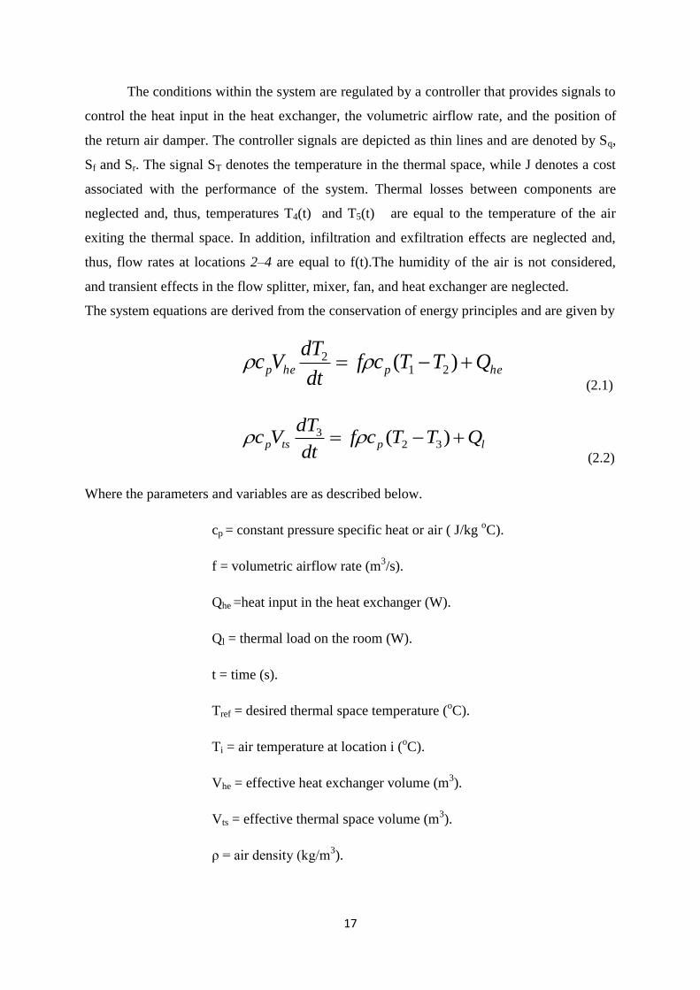
The system equations are derived from the conservation of energy principles and are given by

hephep QTTcfdt

dTVc )( 21

2 (2.1)

lptsp QTTcfdt

dTVc )( 32

3 (2.2)

Where the parameters and variables are as described below.

cp = constant pressure specific heat or air ( J/kg oC).

f = volumetric airflow rate (m3/s).

Qhe =heat input in the heat exchanger (W).

Ql = thermal load on the room (W).

t = time (s).

Tref = desired thermal space temperature (oC).

Ti = air temperature at location i (oC).

Vhe = effective heat exchanger volume (m3).

Vts = effective thermal space volume (m3).

ρ = air density (kg/m3).

18

A lumped capacitance assumption is made, implying that the capacitance of the heat

exchanger and the thermal space are accounted for in the effective heat exchanger and

thermal space volumes. Statements of the conservation of mass and energy applied at the

flow mixer yield

T1 =T3 + ( T0 – T3)/r (2.3)

where r=f ∕ f0 (2.4)

is the system-to-fresh-air volumetric flow-rate ratio. For r=1, there is no recirculation and a

once-through system is considered. The position of the return air damper as described by r is

obtained from the values of f and f0 which are computed explicitly by the controller.

Denoting x=[T2 T3]T and making the appropriate system equations

phe c

uuXXuXT

Vx

1

2123201 )()(1

(2.5)

p

l

ts c

QuXX

Vx

2212 )(

1

(2.6)

Where u= [Qhe, f, f0]T.

2.4 SIMULATION RESULTS

The Heating, Ventilating, and Air-Conditioning (HVAC) Systems are a permanent part of

everyday life in our industrialized society. The single-zone thermal system model shown in

Fig. 2.2 is chosen for our analysis [21]. The system represents a simplification of an overall

building climate control problem, but retains the distinguishing characteristics of an HVAC

system.

The HVAC system state equations shown above (2.5 and 2.6) are solved by Range-

Kutta method. For solving these system equations we considered the different variables and

parameters have taken such as thermal load on the room (Ql), air density (ρ) and etc. Here the

states x1 and x2 are in 0C with respect to time. These two states are identified by using

different structures such as MLP, FLANN and ANFIS. All the simulations are carried out

using MATLAB R2008a. The two desired states x1 and x2 shown in Fig.2.3.

19

Fig.2.3 HVAC System States in 0C

For the purposes of comfort and hygiene, the minimum allowable value of u3, the outside

air volumetric flow rate, is set at 0.0354 m3/ s[22].

The equilibrium states of the system are

3

103

21u

c

uTu

xxp

EQEQ

(2.7)

Since this is an underdetermined case, an infinite number of combinations of u1 and u2

provide the same steady-state output and the system does not possess a unique inverse.

The ranges of the control variables are defined as

Qhe=Є[-4000,4000]W (2.8)

and

f, f0Є[0.0354,2]m3/s. (2.9)

The value of u3 can never exceed the value of u2 , due to conservation of mass principles.

Thus, the controller must command values for these inputs that satisfy the following

condition:

u2 ≥ u3. (2.10)

The operating ranges of the system states and outside air temperature are assumed to be

x1 Є[5,35] 0C or [41,95]

0F (2.11)

x2,T0 Є[10,30] 0C or [50,86]

0F (2.12)

0 10 20 30 40 50 60 70 8010

12

14

16

18

20

22

24Desired states x1 and x2

time

sta

te v

alu

es

x1

x2

20

and the range of the reference temperature is assumed be

Tref Є [17,23] 0C or [62.6, 73.4]

0F (2.13)

In order to most effectively use u3, the controller must have information as to whether the

outside air temperature is higher or lower than the desired room temperature. Thus, an

additional input variable called Tdiff is introduced,

Where

Tdiff = Tref –T0 (2.14)

It is assumed that T0 can be measured accurately with an inexpensive temperature sensor. In

order to determine the ranges of the changes in the states over a sample period of Ts=10 s, the

state equations (3.5) and (3.6) are integrated from 0–10 s, using 1000 random initial

conditions satisfying (3.8)–(3.12). Histograms for Δx1 and Δx2. Based on the extreme values

of Δx1 and Δx2. The ranges for the changes in the states are assumed to be

Δx1 Є [-13.0, 13.0] 0C (2.15)

Δx2 Є [-1.5, 1.5] 0C (2.16)

The range of control signals using assumptions (2.11)–(2.13), (2.15), and (2.16) will be used

to train the neural network to learn the HVAC thermal dynamics.

2.5 HEATING AND COOLING

Heat is energy in the form of molecules in motion. Heat flows from a warmer substance to a

cooler substance. Heat energy flows downhill! Heat does not raise, heated air rises!

Temperature is the level of heat (energy).

The lowest temperature is minus 460°F.

The sun’s temperature is approximately 27,000,000°F.

The temperatures associated with most HVAC systems range from 0°F to 250°F.

Most people feel comfortable if the indoor air temperature is between 68°F and 78°F.

2.5.1 Standard Temperatures on the Fahrenheit and Celsius Scales

Freezing point of (pure) water is:

32 degrees Fahrenheit (32°F) and zero degrees Celsius (0°C).

Boiling point of (pure) water is:

212 degrees Fahrenheit (212°F) and 100 degrees Celsius (100°C).

21

Temperature Conversions for Fahrenheit and Celsius

°C = (°F - 32) ÷ 1.8

°F = 1.8 (°C) + 32

The following is a quick reference for estimating and converting everyday temperatures from

Celsius to Fahrenheit:

0°C is 32°F

16°C is approximately 61°F

28°C is approximately 82°F

37°C is 98.6°F

100°C is 212°F

Absolute Temperatures

The Fahrenheit absolute scale is the Rankine (°R) scale.

The Celsius absolute scale is the Kelvin (°K) scale.

Absolute zero is minus 460°F and 0°R, or minus 273°C and 0°K.

The Fahrenheit/Celsius and the Rankine/Kelvin scales are used interchangeably to describe

equipment and fundamentals of the heating and air conditioning industry.

2.5.2 Heat and Temperature

Heat is energy in the form of molecules in motion. As a substance becomes warmer, its

molecular motion and energy level (temperature) increases. Temperature describes the level

of heat (energy) with reference to no heat. Heat is a positive value relative to no heat.

Because all heat is a positive value in relation to no heat, cold is not a true value. It is really

an expression of comparison. Cold has no number value and is used by most people as a basis

of comparison only. Therefore, warm and hot are comparative terms used to describe higher

temperature levels. Cool and cold are comparative terms used to describe lower temperature

levels. The Fahrenheit scale is the standard system of temperature measurement used in the

United States. However, the U.S. is one of the few countries in the world still using this

system. Most countries use the metric temperature measurement system, which is the Celsius

scale. The Fahrenheit and Celsius scales are currently used interchangeably in the U.S. to

describe equipment and fundamentals in the heating, ventilating and air conditioning

industry.

22

2.5.3 Heat Transfer

Heat naturally flows from a higher energy level to a lower energy level. In other words, heat

travels from a warmer substance to a cooler substance. When there is a temperature

difference between two substances, heat transfer will occur. In fact, temperature difference is

the driving force behind heat transfer. The greater the temperature difference, the greater the

heat transfer.

2.5.4 Types of Heat Transfer

The three types of heat transfer are conduction, convection and radiation.

Conduction

Conduction heat transfer is heat energy traveling from one molecule to another. A heat

exchanger in an HVAC system or home furnace uses conduction to transfer heat. Your hand

touching a cold wall is an example of heat transfer by conduction from your hand to the wall.

However, heat does not conduct at the same rate in all materials. For example, all HVAC

copper conducts at a different rate than iron or aluminum, etc.

Convection

Heat transfer by convection is when some substance that is readily movable such as air,

water, steam, or refrigerant moves heat from one location to another. Compare the words

―convection‖ (the action of conveying) and ―convey‖ (to take or carry from one place to

another). An HVAC system uses convection in the form of air, water, steam and refrigerants

in ducts and piping to convey heat energy to various parts of the system. When air is heated,

it rises; this is heat transfer by ―natural‖ convection. ―Forced‖ convection is when a fan or

pump is used to convey heat in fluids such as air and water. For example, many large

buildings have a central heating plant where water is heated and pumped throughout the

building to the final heated space. Fans then move heated air into the conditioned space.

Radiation

Heat transferred by radiation travels through space without heating the space. Radiation or

radiant heat does not transfer the actual temperature value. The first solid object that the heat

rays encounter absorbs the radiant heat. A portable electric space heater that glows red-hot is

an example of heat transfer by radiation. As the electric heater coil glows red-hot it radiates

heat into the room. The space heater does not heat the air (the space)—instead it heats the

solid objects that come into contact with the heat rays. Any heater that glows has the same

effect. However, radiant heat diminishes by the square of the distance traveled; therefore,

23

space heaters must be placed accordingly. Another good example of radiant heat is the sun;

the sun heats the earth, but not the air around the earth. The sun is also a good example of

diminishing heat. The earth does not experience the total heat of the sun because the sun is

some 93 million miles from the earth.

2.5.5 Ventilating

The ventilation requirement is 1050 cfm. 1050 cfm of outside air is brought in through the

outside air (OA) dampers into the mixed air plenum. This 1050 cfm of outside air mixes with

the 4200 cfm of return air to form 5250 cfm of mixed air, which goes through the coil(s) and

becomes supply air.

2.5.6 Cooling

For this system, the total heat given off by the people, lights and equipment in the

conditioned space plus the heat entering the space through the outside walls, windows, doors,

roof, etc., and the heat contained in the outside ventilation air will be approximately 154,000

Btu/hr. A ton of refrigeration (TR) is equivalent to 12,000 Btu/hr of heat. Therefore, this

HVAC system requires a chiller that can provide approximately 13 tons of cooling (154,000

Btu/hr ÷ 12000 Btu/hr/ton = 12.83 TR) To maintain the proper temperature and humidity in

the conditioned space the cooling cycle is this: The supply air (which is 20°F cooler than the

air in the conditioned space) leaves the cool ing coil and goes through the heating coil (which

is off), through the supply air fan, down the duct and into the conditioned space. The cool

supply air picks up heat in the conditioned space. The warmed air makes its way into the

return air inlets, then into the return air duct and back to the air handling unit. The return air

goes through the return air fan into the mixed air chamber and mixes with the outside air. The

mixed air goes through the filters and into the cooling coil. The mixed air flows through the

cooling coil where it gives up its heat into the chilled water tubes in the coil. This coil also

has fins attached to the tubes to facilitate heat transfer. The cooled supply air leaves the

cooling coil and the air cycle repeats. The water, after picking up heat from the mixed air,

leaves the cooling coil and goes through the chilled water return (CHWR) pipe to the water

chiller’s evaporator. The ―warmed‖ water flows into the chiller’s evaporator—sometimes

called the water cooler—where it gives up the heat from the mixed air into the refrigeration

system. The newly ―chilled‖ water leaves the evaporator, goes through the chilled water

pump (CHWP) and is pumped through the chilled water supply (CHWS) piping into the

cooling coil to pick up heat from the mixed air and the water cycle repeats. The evaporator is

24

a heat exchanger that allows heat from the chilled water return (CHWR) to flow by

conduction into the refrigerant tubes. The liquid refrigerant in the tubes ―boils off‖ to a vapor

removing heat from the water and conveying the heat to the compressor and then to the

condenser. The heat from the condenser is conveyed to the cooling tower through the

condenser water in the condenser return (CWR) pipe. As the condenser water cascades down

the tower, outside air is drawn across the cooling tower removing heat from the water through

the process of evaporation. The ―cooled‖ condenser water falls to the bottom of the tower

basin and is pumped from the tower through the condenser water pump (CWP) and back to

the condenser in the condenser water supply piping (CWS) and the cycle repeats.

2.6 HEATING SYSTEMS

For over 10,000 years, man has used fire to warm himself. In the beginning, interior heating

was just an open fire, but comfort and health was greatly improved by finding a cave with a

hole at the top. Later, fires were contained in hearths or sunken beneath the floor. Eventually,

chimneys were added which made for better heating, comfort, health, and safety and also

allowed individuals to have private rooms. Next, came stoves usually made of brick,

earthenware, or tile. In the 1700s, Benjamin Franklin improved the stove, the first steam

heating system was developed, and a furnace for warm-air heating used a system of pipes and

flues and heated the spaces by gravity flow. In the 1800s, high speed centrifugal fans and

axial flow fans with small, alternating current electric motors became available and high-

pressure steam heating systems were first used. The 1900s brought the Scotch marine boiler

and positive-pressure hydronic circulating pumps that forced hot water through the heating

system. The heating terminals were hot water radiators, which were long, low, and narrow, as

compared to steam radiators, and allowed for inconspicuous heating. Centrifugal fans were

added to furnaces in the 1900s to make forced-air heating systems.

2.7 VENTILATING SYSTEMS

In occupied buildings, carbon dioxide, human odors and other contaminants such as volatile

organic compounds (VOC) or odors and particles from machinery and the process function

need to be continuously removed or unhealthy conditions will result. Ventilation is the

process of supplying ―fresh‖ outside air to occupied buildings in the proper amount to offset

the contaminants produced by people and equipment. In many instances, local building

codes, association guidelines, or government or company protocols stipulate the amount of

25

ventilation required for buildings and work environments. Ventilation systems have been

around for a long time. In 1490, Leonardo da Vinci designed a water driven fan to ventilate a

suite of rooms. In 1660, a gravity exhaust ventilating system was used in the British House of

Parliament. Then, almost two hundred years later, in 1836, the supply air and exhaust air

ventilation system in the British House of Parliament used fans driven by steam engines.

Today, ventilation guidelines are approximately 15 to 25 cfm (cubic feet per minute) of air

volume per person of outside air (OA) for non-smoking areas, 50 cfm for smoking areas.

Ventilation air may also be required as additional or ―make-up‖ air (MUA) for kitchen

exhausts, fume hood exhaust systems, and restroom and other exhaust systems. Maintaining

room or conditioned space pressurization (typically +0.03 to +0.05 inches of water gage) in

commercial and institutional buildings is part of proper ventilation.

Figure 4-10 shows 20% of the total supply air is ventilation outside air (OA) and 80%

is return air (RA). The outside air is brought (or forced) into the mixed air plenum by the

action of the supply air fan. The outside air coming through the outside damper is mixed with

the return air from the conditioned space. The return air dampers control the amount of return

air. If the room pressure is too high, the exhaust air (EA) dampers open to let some of the

return air escape to the outside, which relieves some of the pressure in the conditioned space.

Exhaust air dampers are also called relief air dampers.

2.8 AIR CONDITIONING SYSTEMS

Brooklyn, New York, was the place, and 1902 was the year the first truly successful air

conditioning system for room temperature and humidity control was placed into operation.

But first it took the engineering innovations of Willis Carrier to advance the basic principles

of cooling and humidity control and design the system. Cooling air had already been done

successfully but it was only part of the air conditioning problem. The other part was how to

regulate space humidity. Carrier recognized that drying the air could be accomplished by

saturating it with chilled water to induce condensation. In 1902, Carrier built the first air

conditioner to combat both temperature and humidity. The air conditioning unit was installed

in a printing company and chilled coils were used in the machine to cool the air and lower the

relative humidity to 55%. Four years later, in 1906, Carrier was granted a patent for his air

conditioner the ―Apparatus for Treating Air.‖ However, Willis Carrier did not invent the very

first system to cool an interior structure nor interestingly, did he come up with the term ―air

conditioning.‖ It was Stuart Cramer, a textile engineer, who coined the term ―air

26

conditioning.‖ Mr.Cramer used ―air conditioning‖ in a 1906 patent for a device that added

water vapor to the air. In 1911, Mr. Carrier, who is called the ―father of air conditioning,‖

presented his ―Rational Psychrometric Formulae‖ to the American Society of Mechanical

Engineers. Today, the formula is the basis in all fundamental psychometric calculations for

the air conditioning industry. Though Willis Carrier did not invent the first air conditioning

system, his cooling and humidity control system and psychrometric calculations started the

science of modern psychrometrics and air conditioning. As already mentioned, air ―cooling‖

was only part of the answer. The big problem was how to regulate indoor humidity. Carrier’s

air conditioning invention addressed both issues and has made many of today’s products and

technologies possible. In the 1900s, many industries began to flourish with the new ability to

control the indoor environmental temperature and humidity levels in both occupied and

manufacturing areas. Today, air conditioning is required in most industries and especially in

ones that need highly controllable environments, such as clean environment rooms (CER) for

medical or scientific research, product testing, and sophisticated computer and electronic

Component manufacturing.

CHAPTER 3

SYSTEM IDENTIFICATION USING

ARTIFICIAL NEURAL NETWORKS

28

3.1 INTRODUCTION

Nonlinear system identification of a complex dynamic plant has potential applications in

many areas such as control, communication, power system, instrumentation, pattern

recognition and classification. Because of the function approximation properties and learning

capability, Artificial Neural Networks (ANN’s) have become a powerful tool for these

complex applications. The ANN’s are capable of generating complex mapping between the

input and the output space and thus, arbitrarily complex nonlinear decision boundaries can be

formed by these networks.

An artificial neural network basically consists a number of computing elements,

called neurons that perform the weighted sum of the input signal and the connecting weight.

The sum is added with the bias or threshold and the resultant signal is then passed through a

non-linear element such as tanh(. ) type. Each neuron is associated with three parameters on

whose learning of neuron can be adjusted; these are the connecting weights, the bias and the

slope of the non-linear function. From the structural point of view, a neural network (NN)

may be single layer or it may be multi-layer. In multi-layer structure, there may be more than

one hidden layers and there is one or many artificial neurons in each layer and for a practical

case there may be a number of layers. Each neuron of one layer is connected to each and

every neuron of the next layer.

A neural network is a massively parallel distributed processor made up of simple

processing unit, which has a natural property for storing experimental knowledge and making

it available for use. It resembles the brain in two types

1. Knowledge is acquired by the network from its environment through a learning

process.

2. Interneuron connection strengths, known as synaptic weights, are used to store the

acquired knowledge.

Artificial Neural Networks (ANN) has emerged as a powerful learning technique to

perform complex tasks in highly nonlinear dynamic environments. Some of the prime

advantages of using ANN models are their ability to learn based on optimization of an

appropriate error function and their excellent performance for approximation of nonlinear

function [3]. At present, most of the work on system identification using neural networks are

based on multilayer feed-forward neural networks with back propagation learning or more

efficient variations of this algorithm [18] ,[1].On the otherhand the Functional link

ANN(FLANN) originally proposed by Pao [12] is a single layer structure with functionally

29

mapped inputs. Wang and Chen [19] have presented a fully automated recurrent neural

network (FARNN) that is capable of self-structuring its network in a minimal representation

with satisfactory performance for unknown dynamic system identification and control.

3.2 NEURON STRUCTURE

In 1958, Rosenblatt demonstrated some practical applications using the perceptron [20]. The

perceptron is a single level connection of McCulloch-Pitts neurons sometimes called single-

layer feed-forward networks. The network is capable of linearly separating the input vectors

into pattern of classes by a hyper plane. A linear associative memory is an example of a

single-layer neural network. In such an application, the network associates an output pattern

(vector) with an input pattern (vector), and information is stored in the network by virtue of

modifications made to the synaptic weights of the network.

Fig 3.1 Neuron Structure

The structure of a single neuron is presented in Fig. 3.1. An artificial neuron involves

the computation of the weighted sum of inputs and threshold [3]. The resultant signal is then

passed through a non-linear activation function. The output of the neuron may be represented

as, 𝑦 𝑛 = 𝑓 𝑤𝑗 𝑛 𝑥𝑗 𝑛 + 𝑏 𝑛 𝑁𝑗=1 (3.1)

where, b(n) = threshold to the neuron is called as bias, wj(n) = weight associated with the jth

input, and N = no. of inputs to the neuron.

3.2.1 Activation Functions and Bias

The perceptron internal sum of the inputs is passed through an activation function, which can

be any monotonic function. Linear functions can be used but these will not contribute to a

non-linear transformation within a layered structure, which defeats the purpose of using a

neural filter implementation. A function that limits the amplitude range and limits the output

strength of each perceptron of a layered network to a defined range in a non-linear manner

f(.)

x1

x2

xN

.

.

.

.

b(n)

y(n)

30

will contribute to a nonlinear transformation. There are many forms of activation functions,

which are selected according to the specific problem. All the neural network architectures

employ the activation function [3, 27] which defines as the output of a neuron in terms of the

activity level at its input (ranges from -1 to 1 or 0 to 1). Table 3.1 summarizes the basic types

of activation functions. The most practical activation functions are the sigmoid and the

hyperbolic tangent functions. This is because they are differentiable.

Table 3.1 Types of Activation Functions

The bias gives the network an extra variable and the networks with bias are more powerful

than those of without bias. The neuron without a bias always gives a net input of zero to the

activation function when the network inputs are zero. This may not be desirable and can be

avoided by the use of a bias.

NAME

MATHEMATICAL

REPRESENTATION

Linear 𝑓(𝑥) = 𝑘𝑥

Step 𝑓 𝑥 =

𝛼, 𝑖𝑓 𝑥 ≥ 𝑘𝛽, 𝑖𝑓 𝑥 < 𝑘

Sigmoid 𝑓 𝑥 =

1

1 + 𝑒−𝛼𝑥 ,𝛼 > 0

Hyperbolic

Tangent 𝑓 𝑥 = 1 − 𝑒−𝛾𝑥

1 + 𝑒−𝛾𝑥, 𝛾 > 0

Gaussian 𝑓 𝑥 =

1

2𝜋𝜎2𝑒 − 𝑥−𝜇 2

2𝜎2

31

3.2.2 Learning Technique:

The property that is of primary significance for a neural network is that the ability of the

network to learn from its environment, and to improve its performance through learning. The

improvement in performance takes place over time in accordance with some prescribed

measure. A neural network learns about its environment through an interactive process of

adjustments applied to its synaptic weights and bias levels. Ideally, the network becomes

more knowledgeable about its environment after each iteration of learning process. Hence we

define learning as:

―It is a process by which the free parameters of a neural network are adapted through

a process of stimulation by the environment in which the network is embedded.‖

The processes used are classified into two categories as described in [3]:

(i) Supervised Learning (Learning With a Teacher)

(ii) Unsupervised Learning (Learning without a Teacher)

(i) Supervised Learning:

We may think of the teacher as having knowledge of the environment, with that knowledge

being represented by a set of input-output examples. The environment is, however unknown

to neural network of interest. Suppose now the teacher and the neural network are both

exposed to a training vector, by virtue of built-in knowledge, the teacher is able to provide the

neural network with a desired response for that training vector. Hence the desired response

represents the optimum action to be performed by the neural network. The network

parameters such as the weights and the thresholds are chosen arbitrarily and are updated

during the training procedure to minimize the difference between the desired and the

estimated signal. This updation is carried out iteratively in a step-by-step procedure with the

aim of eventually making the neural network emulate the teacher. In this way knowledge of

the environment available to the teacher is transferred to the neural network. When this

condition is reached, we may then dispense with the teacher and let the neural network deal

with the environment completely by itself. This is the form of supervised learning.

By applying this type of learning technique, the weights of neural network are

updated by using LMS algorithm. The update equations for weights are derived as LMS [3]:

𝑤𝑗 𝑛 + 1 = 𝑤𝑗 𝑛 + 𝜇∆𝑤𝑗 (𝑛) (3.2)

(ii) Unsupervised Learning:

In unsupervised learning or self-supervised learning there is no teacher to over-see the

learning process, rather provision is made for a task independent measure of the quantity of

32

representation that the network is required to learn, and the free parameters of the network are

optimized with respect to that measure. Once the network has become turned to the statistical

regularities of the input data, it develops the ability to form the internal representations for

encoding features of the input and thereby to create new classes automatically. In this

learning the weights and biases are updated in response to network input only. There are no

desired outputs available. Most of these algorithms perform some kind of clustering

operation. They learn to categorize the input patterns into some classes.

3.3 MULTILAYER PERCEPTRON

In the multilayer neural network or multilayer perceptron (MLP), the input signal propagates

through the network in a forward direction, on a layer-by-layer basis. This network has been

applied successfully to solve some difficult and diverse problems by training in a supervised

manner with a highly popular algorithm known as the error back-propagation algorithm [3].

The scheme of MLP using four layers is shown in Fig.3.2. 𝑥𝑖(𝑛) represents the input to the

network, 𝑓𝑗 and 𝑓𝑘 represent the output of the two hidden layers and 𝑦𝑖(𝑛) represents the

output of the final layer of the neural network. The connecting weights between the input to

the first hidden layer, first to second hidden layer and the second hidden layer to the output

layers are represented by respectively

Fig 3.2 Structure of Multilayer Perceptron

First Hidden Layer-2 (Layer-2)

wjk +1 +1

wij

wkl +1

Output signal yi(n)

Input signal xi(n)

Output Layer (Layer-4)

Input Layer (Layer-1)

…

…

… …

…

…

…

…

… Second Hidden Layer (Layer-3)

33

If P1 is the number of neurons in the first hidden layer, each element of the output vector of

first hidden layer may be calculated as,

𝑓𝑗 = 𝜑𝑗 𝑤𝑖𝑗𝑥𝑖 𝑛 + 𝑏𝑗𝑁𝑖=1 , 𝑖 = 1,2,…𝑁, 𝑗 = 1,2,… 𝑃1 (3.3)

where bj is the threshold to the neurons of the first hidden layer, N is the no. of inputs and 𝜑

is the nonlinear activation function in the first hidden layer chosen from the Table 3.1. The

time index n has been dropped to make the equations simpler. Let P2 be the number of

neurons in the second hidden layer. The output of this layer is represented as, fk and may be

written as

𝜑𝑘 𝑤𝑗𝑘 𝑓𝑗 + 𝑏𝑘𝑃1𝑗=1 ,𝑘 = 1,2,… .𝑃2 (3.4)

where, bk is the threshold to the neurons of the second hidden layer. The output of the final

output layer can be calculated as

𝑦𝑙 𝑛 = 𝜑𝑙 𝑤𝑘𝑙𝑓𝑘 + 𝑏𝑙𝑃2𝑘=1 , 𝑙 = 1,2,… 𝑃3 (3.5)

where, bl is the threshold to the neuron of the final layer and P3 is the no. of neurons in the

output layer. The output of the MLP may be expressed as

𝑦𝑙 𝑛 = 𝜑𝑙 𝑤𝑘𝑙 𝜑𝑘 𝑤𝑗𝑘 𝜑𝑗 𝑤𝑖𝑗𝑥𝑖 𝑛 + 𝑏𝑗𝑁𝑖=1 + 𝑏𝑘

𝑃1𝑗=1 + 𝑏𝑙

𝑃2𝑘=1 (3.6)

3.3.1 Back Propagation Algorithm

Fig 3.3 Neural Network with Back Propagation Algorithm

An MLP network with 2-3-2-1 neurons (2, 3, 2 and 1 denote the number of neurons in the

input layer, the first hidden layer, the second hidden layer and the output layer respectively)

Back-Propagation Algorithm

x1

x2 yl(n)

dl(n)

el(n)

+

-

34

with the back-propagation (BP) learning algorithm, is depicted in Fig.3.3. The parameters of

the neural network can be updated in both sequential and batch mode of operation. In BP

algorithm, initially the weights and the thresholds are initialized as very small random values.

The intermediate and the final outputs of the MLP are calculated by using (3.3), (3.4), and

(3.5.) respectively. The final output 𝑦𝑙(𝑛) at the output of neuron l, is compared with the

desired output 𝑑 𝑛 and the resulting error signal 𝑒 𝑛 is obtained as

𝑒𝑙 𝑛 = 𝑑 𝑛 − 𝑦𝑙 𝑛 (3.7)

The instantaneous value of the total error energy is obtained by summing all error

signals over all neurons in the output layer, that is

𝜉 𝑛 = 1

2 𝑒𝑙

2(𝑛)𝑃3𝑙=1 (3.8)

where P3 is the no. of neurons in the output layer.

This error signal is used to update the weights and thresholds of the hidden layers as

well as the output layer. The reflected error components at each of the hidden layers is

computed using the errors of the last layer and the connecting weights between the hidden

and the last layer and error obtained at this stage is used to update the weights between the

input and the hidden layer. The thresholds are also updated in a similar manner as that of the

corresponding connecting weights. The weights and the thresholds are updated in an iterative

method until the error signal become minimum. For measuring the degree of matching,

Squared error cannot be considered as the network may have multiple outputs and Root Mean

Square Error (RMSE) cause over fitting of the model and the weights may not converge. So

the Mean Square Error (MSE) is taken as a performance measurement.

The weights are using the following formulas,

𝑤𝑘𝑙 𝑛 + 1 = 𝑤𝑘𝑙 𝑛 + ∆𝑤𝑘𝑙 𝑛 (3.9)

𝑤𝑗𝑘 𝑛 + 1 = 𝑤𝑗𝑘 𝑛 + ∆𝑤𝑗𝑘 𝑛 (3.10)

𝑤𝑖𝑗 𝑛 + 1 = 𝑤𝑖𝑗 𝑛 + ∆𝑤𝑖𝑗 𝑛 (3.11)

∆𝑤𝑘𝑙 𝑛 = −2𝜇𝜕𝜉 (𝑛)

𝜕𝑤𝑘𝑙 𝑛 = 𝜇𝑒(𝑛)

𝑑𝑦 𝑙(𝑛)

𝑑𝑤𝑘𝑙 𝑛

= 𝜇𝑒(𝑛)𝜑𝑙′ 𝑤𝑘𝑙𝑓𝑘 + 𝑏𝑙

𝑃2

𝑘=1 𝑓𝑘 (3.12)

where, µ is the convergence coefficient (0<µ<1). Similarly ∆𝑤𝑗𝑘 𝑛 and ∆𝑤𝑖𝑗 𝑛 the can be

computed [3]. The thresholds of each layer can be updated in a similar manner, i.e.

35

𝑏𝑙 𝑛 + 1 = 𝑏𝑙 𝑛 + ∆𝑏𝑙 𝑛 (3.13)

𝑏𝑘 𝑛 + 1 = 𝑏𝑘 𝑛 + ∆𝑏𝑘 𝑛 (3.14)

𝑏𝑗 𝑛 + 1 = 𝑏𝑗 𝑛 + ∆𝑏𝑗 𝑛 (3.15)

where, ∆𝑏𝑙 𝑛 ,∆𝑏𝑘 𝑛 and ∆𝑏𝑗 𝑛 are the change in thresholds of the output, hidden and

input layer respectively. The change in threshold is represented as,

∆𝑏𝑙 𝑛 = −2𝜇 𝜕𝜉(𝑛)𝜕𝑏𝑙 𝑛

= 𝜇𝑒(𝑛)𝑑𝑦𝑙(𝑛)

𝑑𝑏𝑙 𝑛

= 𝜇𝑒(𝑛)𝜑𝑙′ 𝑤𝑘𝑙𝑓𝑘 + 𝑏𝑙

𝑃2

𝑘=1 (3.16)

From the structural point of MLP, it is very complex and it there are more than two

hidden layers the structure becomes more complex. As more number of weights are present

when implemented in DSP or FPGA memory requirements are considered and during

updation of weights in Back Propagation it becomes very complex thereby causing over

burden on the processor used. So a very simple and powerful structure is required and thus

FLANN is considered.


The MLP structure considered for simulation purpose is shown in Fig.3.2. A three-layer MLP

structure with single hidden layer with three nodes and one input node and one output node

was chosen for the purpose of identification. tanh(.) function is taken as an activation

function for the given structure. The BP algorithm is used to adapt the weights of MLP

structure. The input u is a uniform distributed signal, called volumetric air flow rate (m3/sec),

in the interval [0, 80] with 1000 samples. The convergence parameter set to 0.001 for MLP

weight updating. 80 iterations are taken for structure updation, after which the weights of the

ANN is stored for testing. For testing, the input signal is taken from the volumetric air flow

rate (with 200) samples in the interval [20 40]. After the simulation, in the training part the

error approached to zero as shown in the figures 3.5 and 3.7 for two states respectively. In

these figure, the mean square error (MSE) is plotted over the 80 iterations. In the testing part,

the estimated (MLP model) output is matched to desired (Plant) output. The graphs for

response matching are shown in figures 3.4 and 3.6 for given two states (x1 and x2) testing

samples, respectively.

36

Fig. 3.4 HVAC System single (x1) state in

0C

Fig.3.5. Mean square error of HVAC System x1 state.

Fig. 3.6 HVAC System single (x2) state in 0C

20 22 24 26 28 30 32 34 36 38 4010

12

14

16

18

20

22

24

Time

Sta

te V

alu

e (

x1)

Plant

MLP model

0 10 20 30 40 50 60 70 800

5

10

15

20

iterations

MS

E

MLP-BP

20 22 24 26 28 30 32 34 36 38 4013

14

15

16

17

18

19

20

21

Time

Sta

te V

alu

e (

x2)

Plant

MLP model

37

Fig.3.7 Mean square error of HVAC System x2 state.

3.5 FUNCTIONAL LINK ANN

Pao originally proposed FLANN and it is a novel single layer ANN structure capable of

forming arbitrarily complex decision regions by generating nonlinear decision boundaries

[12]. Here, the initial representation of a pattern is enhanced by using nonlinear function and

thus the pattern dimension space is increased. The functional link acts on an element of a

pattern or entire pattern itself by generating a set of linearly independent function and then

evaluates these functions with the pattern as the argument. Hence separation of the patterns

becomes possible in the enhanced space. The use of FLANN not only increases the learning

rate but also has less computational complexity. Pao et al [20] have investigated the learning

and generalization characteristics of a random vector FLANN and compared with those

attainable with MLP structure trained with back propagation algorithm by taking few

functional approximation problems. A FLANN structure with two inputs is shown in Fig. 3.4.

3.5.1 Learning Algorithm

Let X is the input vector of size N×1 which represents N number of elements; the kth

element

is given by:

𝑋 𝑘 = 𝑥𝑘 , 1 ≤ 𝑘 ≤ 𝑁 (3.17)

Each element undergoes nonlinear expansion to form M elements such that the

resultant matrix has the dimension of N×M. The functional expansion of the element xk by

power series expansion is carried out using the equation given in (3.18)

𝑠𝑖 = 𝑥𝑘 𝑓𝑜𝑟 𝑖 = 1

𝑥𝑘𝑙 𝑓𝑜𝑟 𝑖 = 2,3,…𝑀

(3.18)

0 10 20 30 40 50 60 70 800

5

10

15

20

iterations

MS

E

MLP-BP

38

where l = 1,2,3, … M. For trigonometric expansion, the

𝑠𝑖 =

𝑥𝑘 𝑓𝑜𝑟 𝑖 = 1

sin 𝑙𝜋𝑥𝑘 𝑓𝑜𝑟 𝑖 = 2,4,… ,𝑀

cos 𝑙𝜋𝑥𝑘 𝑓𝑜𝑟 𝑖 = 3,5, . . . ,𝑀 + 1

(3.19)

where l = 1,2,3, … M. In matrix notation the expanded elements of the input vector E, is

denoted by S of size N×(M+1). The bias input is unity. So an extra unity value is padded with

the S matrix and the dimension of the S matrix becomes N×Q, where Q = M+2.

Fig. 3.8 Structure of FLANN

Let the weight vector is represented as W having Q elements. The output is given as

𝑦 = 𝑠𝑖𝑤𝑖𝑄𝑖=1 (3.20)

In matrix notation the output can be,

𝑌 = 𝑆.𝑊𝑇 (3.21)

At nth

iteration the error signal 𝑒(𝑛) can be computed as

𝑒 𝑛 = 𝑑 𝑛 − 𝑦(𝑛) (3.22)

Let 𝜉 𝑛 denotes the cost function at iteration k and is given by

𝜉 𝑛 = 1

2 𝑒𝑗

2(𝑛)𝑃𝑗=1 (3.23)

where P is the number of nodes at the output layer. The weight vector can be updated by least

mean square algorithm, as

𝑤 𝑛 + 1 = 𝑤(𝑛) −𝜇

2∆ 𝑛 (3.24)

where ∆ 𝑛 is an instantaneous estimate of the gradient 𝜉 𝑛 of with respect to the weight

vector 𝑤 𝑛 . Now

Fu

nct

ion

al

Exp

an

sio

n

Adaptive Algorithm

S

x2

yl(n)

dl(n)

el(n)

+

-

x1

1

W

39

∆ 𝑛 = 𝜕𝜉𝜕𝑤

= −2𝑒 𝑛 𝜕𝑦 𝑛

𝜕𝑤= −2𝑒 𝑛

𝜕 𝑤 𝑛 𝑠(𝑛)

𝜕𝑤

= −2𝑒 𝑛 𝑠(𝑛) (3.25)

Substituting the value of (4.25) in (4.24) we get

𝑤 𝑛 + 1 = 𝑤(𝑛) − 𝜇𝑒 𝑛 𝑠(𝑛) (3.26)

where 𝜇 denotes the step-size 0 ≤ 𝜇 ≤ 1 which controls the convergence speed of the LMS

algorithm.

The functions used for Functional Expansion is linearly independent and this may be

achieved by the use of suitable orthogonal polynomials for functional expansion. The

trigonometric polynomial basis functions provide a compact representation of the function in

the mean square sense. However, when the outer product terms were used along with the

trigonometric polynomials for functional expansion, better results were obtained in the case

of learning of a two-variable function.


For the simulation purpose FLANN structure with single input node and single output node is

taken. In this structure, the input pattern is expanded by using trigonometric polynomials, i.e.,

by using cos 𝑛𝜋𝑢 and sin 𝑛𝜋𝑢 , for n = 1, 2. One bias and one direct input are also taken in

the function expansion. Thus, it has only 6 weights in the structure which are to be updated in

each iteration. Least square method is used for weight updation. The input u is a uniform

distributed signal, called volumetric air flow rate (m3/sec), in the interval [0, 80] with 1000

samples. 80 iterations are taken for structure updation, after which the weights of the ANN is

stored for testing. For testing, the input signal is taken from the volumetric air flow rate (with

200) samples in the interval [0 80]. After the simulation, in the training part the error

approached to zero as shown in the figures 3.10 and 3.12 for two states (x1 and x2)

respectively. In these figures, the mean square error (MSE) is plotted over the 80 iterations.

In the testing part, the estimated output is matched to desired output. The graphs for response

matching are shown in figures 3.9 and 3.11 for given two states testing samples, respectively.

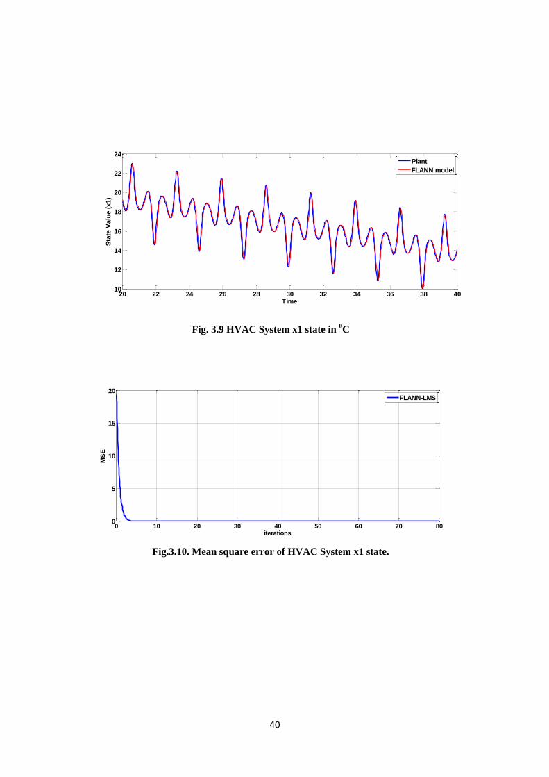
40

Fig. 3.9 HVAC System x1 state in 0C


20 22 24 26 28 30 32 34 36 38 4010

12

14

16

18

20

22

24

Time

Sta

te V

alu

e (

x1)

Plant

FLANN model

0 10 20 30 40 50 60 70 800

5

10

15

20

iterations

MS

E

FLANN-LMS

41

Fig. 3.11 HVAC System x2 state in 0C


20 22 24 26 28 30 32 34 36 38 4013

14

15

16

17

18

19

20

Time

Sta

te V

alu

e (

x2)

Plant

FLANN model

0 10 20 30 40 50 60 70 800

5

10

15

20

iterations

MS

E

FLANN-LMS

CHAPTER 4

MODIFIED BP AND BP ALGORITHMS

43

4.1 INTRODUCTION

Emotion tends to be used in clinical terminology for what a person is feeling at a given

moment. Joy, sadness, anger, fear, disgust, and surprise are often considered the six most

basic emotions, and other well-known human emotions (e.g., pride, shame, regret, elation,

etc.) are often treated as elaborations or specializations of these six to complex social

situations. Recent definitions of emotion have either emphasized the external stimuli that

trigger emotion, or the internal responses involved in the emotional state, when in fact

emotion includes both of those things and much more [23]. According to Perlovsky [24], [25]

emotions refer to both exaggeratedly expressive communications and to internal states related

to feelings. Love, hate, courage, fear, joy, sadness, pleasure, and disgust can all be described

in both psychological and physiological terms. Emotion is the realm where thought and

physiology are inextricably entwined, and where the self is inseparable from individual

perceptions of value and judgment toward others and ourselves. Emotions are sometimes

regarded as the antithesis of reason. A distinctive and challenging fact about human beings is

a potential for both opposition and entanglement between will, emotion, and reason.

Recently, Abu Maria and Abu Zitar [29] proposed and implemented a regular and an

emotional agent architecture, which is supposed to resemble some of the human behaviors.

They noticed that artificial emotions can be used in different ways to influence decision

making. Moreover, Gobbini and Haxby [30] proposed a model for distributed neural systems

that participate in the recognition of familiar faces, highlighting that this spatially distributed

process involves not only visual areas but also areas that primarily have cognitive and social

functions such as person knowledge and emotional responses.

In summary, many researchers have attempted incorporating emotions into AI for

different aims and reasons. Perhaps the common question among all these works and also the

work that is presented within this paper is as follows: Should we, and can we, develop

machines with feelings?

The answer to the first part is yes, we should have emotional and intelligent machines.

Several researchers (e.g., [24] and [31]) suggested that passion, emotion, or feeling can add

backing to an argument, even one based primarily on reason, and that typically there is no

thought based ―purely‖ on intellectual logic or ―purely‖ on emotion—most decisions and

cognitions are founded on a mixture of both. In fact decisions and cognitions can be greatly

influenced by the emotional state, as described in [27]: ―The specific effects on attention and

cognition of a number of affective states have been studied extensively (e.g. anxiety and fear,

44

anger and frustration, positive and negative affect, etc.). These effects include altering the

nature of attentional processing (e.g. changes in attention capacity, speed and bias); helping

to activate (or inhibit) particular perceptual and cognitive schemas that enhance (or limit) the

perception and processing of specific stimuli.‖ Therefore, having emotional machines not

only gets us closer to modeling humans, but also aids in improving the decision making

process of these machines.

The answer to the second part is yes and no. Yes we can have emotional intelligent

machines, if we accept that their emotions are not exactly human, but rather simulation of

some emotions that appear to model apparent human external emotions or their perception by

other humans; and no, we cannot have emotional robots if we expect them to have human-

like emotions and feelings— for the simple reason that we are still unsure about what

constitutes the essence of emotions. The motivation for the work in this paper comes from

our belief that we can have certain human emotions artificially modeled in machines.

Previous works on modeling different emotions suggested that this is conceivable. However,

with the existence of many emotions that vary in response from one human to another, even

with similar input stimuli, we choose to model specific emotional parameters with the

objective of improving the learning capability of a ―nonhuman‖ system. The system here is

based on a supervised neural network that uses the back propagation (BP) learning algorithm.

Therefore, our aim in this paper is to model simulated emotions within a simple

supervised neural network structure, and to investigate the effect of the added emotional

factors on the learning and decision making capabilities of the neural network.

We only consider two emotions (anxiety and confidence), which we believe have an

effect on learning and decision making in humans. In our hypothesis (think of children

learning new tasks), when we learn a new task, the anxiety level is high at the beginning and

the confidence level is low. After time, practice and getting positive feedback, the anxiety

level decreases while the confidence level increases. Once learning is achieved, we tend to be

less anxious and more confident performing a task that we have already experienced.

Therefore, anxiety and confidence are two dependent dimensions, where confidence is

defined as the negative rate of change of anxiety.

Anxiety is a physiological state characterized by cognitive, somatic, emotional, and

behavioral components. These components combine to create the feelings that we typically

recognize as fear, apprehension, or worry. Anxiety is not always pathological or maladaptive:

it is a common emotion along with fear, anger, sadness, and happiness.

45

Confidence is described as a state of being certain, either that a hypothesis or

prediction is correct, or that a chosen course of action is the best or most effective given the

circumstances. Confidence can be described as a subjective, emotional state of mind, but is

also represented statistically as a confidence level within which one may be certain that a

hypothesis will either be accepted or rejected.

In our work, we refer to anxiety and confidence as ―emotions,‖ however, one could

argue whether they are genuine human emotions. The definition of anxiety describes it as a

common emotion, however we may also consider it as an emotional state of mind or

emotional response that may not be related to any biological processes in the brain. Similarly

for confidence, it is considered as an emotional state of mind, an emotional response, or an

emotion as we call it, because it has an emotional effect on the learning process.

In this paper, we propose a new emotional back propagation (EmBP) learning

algorithm based on incorporating two essential emotions (anxiety and confidence) during the

processes of learning and decision making. The distinctive, emotion-related elements of

EmBP are twofold. First, there is pattern averaging, which attempts mimicking the tendency

for human emotional judgments and preferences to be based on general impressions

XIi YIi

Input layer neuron

Fig 4.1 Input/output configuration of an input-layer neuron

rather than precise details of the objects being perceived. Second, there are the confidence

and anxiety variables, which are influenced by the perceived objects: ―Indeed, anger or fear

can often be thought of as a systematic response to observed facts [24].‖ This paper suggests

that these two emotional responses can be successfully simulated and used during the training

of a supervised neural network with the purpose of providing more effective learning. The

two emotional variables are dependent on each other, where confidence is measured as the

difference between anxiety levels at two different iterations.

i

46

4.2 EMOTIONAL BACK PROPAGATION LEARNING ALGORITHM

In 1986, Rumelhart et al. proposed a generalized delta rule known as BP for training layered

neural networks. This algorithm has been popularly used ever since due to its implementation

simplicity and quick training, specially, when sufficient training database is available. In this

section, the modification of this algorithm, by adding two emotional coefficients, provides

the proposed EmBP, which will be explained in details according to the flow of information

within the neural network, which consists of three layers: input layer with (4.2.1) neurons,

hidden layer with (h) neurons, and output layer with (j) neurons.

4.2.1 Input-Layer Neurons

These are not processing neurons, thus, the output of each input-layer neuron is defined as

YIi=XIi 4.1)

where XIi and YIi are, respectively, the input and output values of neuron in the input layer.

Fig. 4.1 shows the input and output configuration of an input-layer neuron.

Fig. 4.2 Input/output configuration of a hidden-layer neuron

4.2.2 Hidden-Layer Neurons

These are processing neurons; therefore, the sigmoid activation function is used to activate

each neuron in this layer. Here it is assumed that there is one hidden layer, however the same

process can be applied for more than one hidden layer using the following algorithm. The

output of each hidden-layer neuron is defined as

YHh=

)exp(1

1

hXH (4.2)

47

where XHh and YHh are the input and output values of neuron h in the hidden layer,

respectively. The input to a hidden-layer neuron XHh is calculated using the total potential

(TPh ) of all input values coming into that neuron. The total potential is the sum of

multiplications of input values and their associated weights. There are three different groups

of inputs, and consequently, types of total potential, coming into a hidden-layer neuron. The

first total potential (TPhc) is the conventional total potential, which is obtained using the

output values of the previous layer (input layer, in this case) and the conventional weight

matrix. The second total potential (TPhb) is obtained using the hiddenlayer bias neuron and its

associated weights. The third total potential (TPhm) is obtained using the hidden-layer

emotional neuron and its associated weights. Therefore,the input to a hidden-layer neuron is

defined as

hmhbhch TPTPTPXH (4.3)

TPhc is defined as

i

r

i

hihc YIWTP

1 (4.4)

Where Whi is the weight given by hidden neuron h to input Neuron i , and YIi is the output of

input neuron i.r is the maximum number of input-layer neurons. TPhb is defined as

bhbhb XWTP (4.5)

where Whb is the weight given by hidden neuron h to the hidden-layer bias neuron b , Xb and

is the input value to the bias neuron, which is set to 1(Xb=1).

TPhm is defined as

mhmhm XWTP (4.6)

where Whm is the weight given by hidden neuron h to the hidden-layer emotional neuron m ,

and Xm is the input value to the emotional neuron. Xm represents the input pattern average

value, which in our hypothesis affects the learning of the neural network. According to

Baumgartner et al. ―Most of the published neuroimaging papers examining emotional

processes have used visual stimuli in order to evoke emotions (positive or negative).‖

Therefore, the global average of an input pattern is fed into the emotional neuron and the

resulting total potential is used to calculate the output of the hidden layer.

48

Xm is calculated as

Xm=YPAT (4.7)

Where YPAT is the global input pattern average value for an input Image P(x,y)

YPAT =

maxmax,

1,1

),(

yx

yx

yxP /xmax.ymax (4.8)

Where xmax and ymax are the highest number of pixels in the x and y directions of image

P(x,y) , respectively. Fig.4.2 shows the input and output configuration of a hidden-layer

neuron.

4.2.3 Output-Layer Neurons

These are also processing neurons, and similarly to the hidden layer, the sigmoid activation

function is used to activate each neuron in this layer.

The output of each output-layer neuron is defined as

)exp(1

1

j

jXJ

YJ

(4.9)

where XJj and YJj are the input and output values of neuron j in the output layer, respectively.

The input to an output-layer neuron XJj is also calculated using the total potential

(TPj) of all input values coming into that neuron from the previous hidden layer and the bias

and emotional neurons.Therefore, the input to an output-layer neuron is defined as

jmjbjcj TPTPTPXJ (4.10)

Fig 4.3 Input/Output configuration of an output-layer neuron

49

TPjc is defined as

h

l

h

jhjc YHWTP

1 (4.11)

where Wjh is the weight given by output neuron j to hidden neuron h, and YHh is the output

of hidden neuron h .l is the maximum number of hidden-layer neurons.

TPjb is defined as

bjbjb XWTP (4.12)

where Wjb is the weight given by output neuron j to the outputlayer bias neuron b , and Xb is

the input value to the bias neuron, which is set to 1(Xb=1).

TPjm is defined as

mjmjm XWTP (4.13)

where Wjm is the weight given by output neuron j to the outputlayer emotional neuron m, and

Xm is the input value to the emotional neuron. Xm is calculated as in (4.7). Fig. 4.3 shows the

input and output configuration of an output-layer neuron.

4.2.4 The Emotional Back propagation Parameters

Here the proposed emotional parameters are used together with the existing learning

coefficient (η) and momentum rate (α) in order to adjust the neural network weights, based on

error minimization.

The proposed emotional parameters are the anxiety coefficient (µ) and the confidence

coefficient (k). According to our hypothesis, when we learn a new task, the anxiety level is

high at the beginning and the confidence level is low. After time, practice, and getting

positive feedback, the anxiety level decreases while the confidence level increases. Once

learning is achieved, we tend to be less anxious and more confident doing a task that we have

already learned. The proposed emotional neural network incorporates both emotional

coefficients during the learning and the generalization processes. Both coefficients have

values between ―0‖ and ―1.‖ In order to model the emotional factor in an artificial neural

network, the following assumptions are made.

Assumption 1: The anxiety level is dependent on the input patterns, where new

patterns cause higher anxiety. During the first iteration (new task learning), the initial anxiety

coefficient value is set to ―1.‖

50

Assumption 2: The anxiety level is dependent on the difference (error) between the

actual output of the neural network and the desired (target) output. This is a kind of feedback

that the emotional neural network uses to measure how successful its learning is. Anxiety

decreases with the minimization of the error.

Assumption 3: The confidence level increases with the decrease in anxiety level.

During the first iteration (new task learning), the initial confidence coefficient value is set to

―0.‖ Based on the above assumptions, the anxiety coefficient (µ) value is defined as

EYAvPAT (4.14)

where YAvPAT is the average value of all presented patterns to the neural network in each

iteration, which is defined as

NYYpN

p

PATAvPAT

1

(4.15)

where p is pattern index from first to the last pattern Np .YPAT is the average value of pattern

p. The error feedback E is defined as

jp

N

j

jj NNYJTEj

1

2)(

(4.16)

where j is the output neuron index from first to the last neuron Nj and Np is the total number

of patterns. YJj and Tj are the actual and target output value for neuron j, respectively. The

confidence coefficient (k) value is defined as

iok

(4.17)

where (µ0) is the anxiety coefficient value after the first iteration (exposure to new patterns)

and (µi) is the anxiety coefficient value in at subsequent iteration i.

51

4.3 BACK PROPAGATION WEIGHT UPDATE RULE

This idea was first described by Werbos [32] and popularised by Rumelhart et al.[33].

i

n

p „P red‟

u

t

s

Fig 4.4 A multilayer perceptron

Consider the network above, with one layer of hidden neurons and one output neuron.

When an input vector is propagated through the network, for the current set of weights there

is an output Pred. The objective of supervised training is to adjust the weights so that the

difference between the network output Pred and the required output Req is reduced. This

requires an algorithm that reduces the absolute error, which is the same as reducing the

squared error, where:

Network Error = Pred – Req

= E (4.18)

The algorithm should adjust the weights such that E2 is minimised. Back-propagation

is such an algorithm that performs a gradient descent minimisation of E2.

f()

f()

f()

f()

f()

Neurons

Weights

http://www.philbrierley.com/code/bpproof.html#ref3

52

In order to minimize E2, its sensitivity to each of the weights must be calculated. In

other words, we need to know what effect changing each of the weights will have on E2. If

this is known then the weights can be adjusted in the direction that reduces the absolute error.

The notation for the following description of the back-propagation rule is based on

the diagram below.

1O BW1

2O BW2 BO

nO nBW

Fig 4.5 Notations for back propagation rule

The dashed line represents a neuron B, which can be either a hidden or the output neuron.

The outputs of n neurons (O 1 ...O n ) in the preceding layer provide the inputs to neuron B. If

neuron B is in the hidden layer then this is simply the input vector.

These outputs are multiplied by the respective weights (W1B...WnB), where WnB is the

weight connecting neuron n to neuron B. The summation function adds together all these

products to provide the input, IB, that is processed by the activation function f (.) of neuron

B. f (IB) is the output, OB, of neuron B.

For the purpose of this illustration, let neuron 1 be called neuron A and then consider

the weight WAB connecting the two neurons.

The approximation used for the weight change is given by the delta rule:

AB

oldABnewABW

EWW

2

)()( (4.19)

where η is the learning rate parameter, which determines the rate of learning, and

ABW

E

2

Summation function activation function

BI

Neuron B

1X

nX

XBXWO

)( BIf

53

is the sensitivity of the error, E2, to the weight WAB and determines the direction of search in

weight space for the new weight WAB(new) as illustrated in the figure below.

Fig 4.6 In order to minimize E2 the delta rule gives the direction of weight change required

From the chain rule,

AB

B

BAB W

I

I

E

W

E

22

(4.20)

and AB

x

nx

xBx

AB

B

W

WO

W

I

1

AB

x

nX

xBx

AB

ABA

W

WO

W

WO

2

)(

=OA (4.21)

Since the rest of the inputs to neuron B have no dependency on the weight WAB.Thus from

eqns. (5.20) and (5.21), eqn. (5.19) becomes,

A

B

oldABnewAB OI

EWW

2

)()( (4.22)

and the weight change of WAB depends on the sensitivity of the squared error, E2, to the nput,

IB, of unit B and on the input signal OA.

54

There are two possible situations:

1. B is the output neuron;

2. B is a hidden neuron.

Considering the first case:

Since B is the output neuron, the change in the squared error due to an adjustment of WAB is

simply the change in the squared error of the output of B:

22 )Re(Pr qedE

BB I

edqed

I

E

Pr)Re(Pr2

2

B

B

I

IfE

)(2

)(2 BIfE (4.23)

Combining eqn. (4.22) with (4.23) we get,

)(2)()( BAoldABnewAB IfEOWW (4.24)

The rule for modifying the weights when neuron B is an output neuron.

If the output activation functions, f (.), is the logistic function then:

1)1(

1

1)(

x

xe

exf (4.25)

differentiating (4.25) by its argument x

2

2

)1()(1)1(1)(

x

xxx

e

eeexf

(4.26)

But, xe

xf

1

1)(

(4.27)

)(/))(1( xfxfe x (4.28)

55

Inserting (4.28) into (4.26) gives:

2))((

1)(

))(1(

)('

xf

xf

xf

xf

))(1()( xfxf (4.29)

similarly for the tanh function,

))(1()( 2xfxf

or for the linear (identity) function,

1)( xf

This gives:

)....(log).........1(2)()( isticOEOOWW BBAoldABnewAB

....(tanh)).........1(22

)()( BAoldABnewAB OEOWW

).....(....................2)()( linearEOWW AoldABnewAB

Considering the second case:

B is a hidden neuron.

B

B

BB I

O

O

I

I

E

I

E

0

0

22

(4.30)

where the subscript, o, represents the output neuron.

)()(

B

B

B

B

B IfI

If

I

O

(4.31)

56

B

p

p

p

B O

WO

O

I

0

0 (4.32)

where p is an index that ranges over all the neurons including neuron B that provide input

signals to the output neuron. Expanding the right hand side of equation (4.32),

0

0

0

0

B

B

Bp

p

Pp

B

BB

B

p

p

p

WO

WO

O

WO

O

WO

(4.33)

since the weights of the other neurons ,WpO (p!=B) have no dependency on OB.

Inserting (4.31) and (4.33) into (4.30),

)(0

0

22

BB

B

IfWI

E

I

E

(4.34)

Thus BI

E

2

is now expressed as a function of 0

2

I

E

, calculated as in (4.23).

The complete rule for modifying the weight WAB between a neuron A sending a signal to a

neuron B is,

A

B

oldABnewAB OI

EWW

2

)()(

(4.35)

where, )(2 0'

2

B

B

IEfI

E

-IB is the output newron (4.36)

)(0

22

BkBO

B

IfWI

E

I

E

-IB is the hidden newron (4.37)

where fo(.) and fh(.)are the output and hidden activation functions respectively.

57


The MLP structure considered for simulation purpose is shown in Fig.3.2. A three-layer MLP

structure with single hidden layer with three nodes and one input node and one output node

was chosen for the purpose of identification. tanh(.) function is taken as an activation

function for the given structure. The Modified Back Propagation (MBP) algorithm is used to

adapt the weights of MLP structure. The input u is a uniform distributed signal, called

volumetric air flow rate (m3/sec), in the interval [0, 80] with 1000 samples. The convergence

parameter set to 0.001 for MLP weight updating. 80 iterations are taken for structure

updation, after which the weights of the ANN is stored for testing. For testing, the input

signal is taken from the volumetric air flow rate (with 200) samples in the interval [20 40].

After the simulation, in the training part the error approached to zero as shown in the figures

4.8 and 4.10 for two states respectively. In these figure, the mean square error (MSE) is

plotted over the 80 iterations. In the testing part, the estimated (MLP model) output is

matched to desired (Plant) output. The graphs for response matching are shown in figures 4.7

and 4.9 for given two states (x1 and x2) testing samples, respectively.

Fig.4.7 HVAC System x1 state in 0C

20 22 24 26 28 30 32 34 36 38 4010

12

14

16

18

20

22

24

Time

Sta

te V

alu

e (

x1)

Plant

MLP model

58



Fig. 4.10 Mean square error of HVAC System x2 state.

0 10 20 30 40 50 60 70 800

5

10

15

20

iterations

MS

E

MLP-MBP

20 22 24 26 28 30 32 34 36 38 4013

14

15

16

17

18

19

20

Time

Sta

te V

alu

e (

x2)

Plant

MLP model

0 10 20 30 40 50 60 70 800

5

10

15

20

iterations

MS

E

MLP-MBP

59

4.5 COMPARISON OF RESULTS

The Mean Square Errors (MSE) for HVAC system state x1 are compared for different ANN

structures, and shown below in Fig.4.11. Among all these errors the MLP-MBP error is very

fast converging comparing other techniques and it contains less error and less computation

time shown in table No 4.1. The FLANN-LMS error is converging slowly with respect to

MLP-MBP and fast converging with respect to MLP-BP and computational time value is in

between these two techniques shown in table No 4.1. The MLP-BP error is very slowly

converging, comparing MLP-BP and FLANN-LMS errors, and computational time also very

high shown in table No 4.1. So in all these techniques the MLP-MBP technique is very good.

All the simulations are carried out using MATLAB R2008a.


The Mean Square Errors (MSE) for HVAC system state x2 are compared for different

ANN structures, and shown below in Fig.4.12. Among all these errors the MLP-MBP error is

very fast converging comparing other techniques and it contains less error and less

computation time shown in table No 4.1. The FLANN-LMS error is converging slowly with

respect to MLP-MBP and fast converging with respect to MLP-BP and computational time

value is in between these two techniques shown in table No 4.1. The MLP-BP error is very

slowly converging, comparing MLP-BP and FLANN-LMS errors, and computational time

also very high shown in table No 4.1. So in all these techniques the MLP-MBP technique is

very good. All the simulations are carried out using MATLAB R2008a.

0 10 20 30 40 50 60 70 800

5

10

15

20

iterations

MS

E

MLP-BP

MLP-MBP

FLANN-LMS

60


4.6 PERFORMANCE OF DIFFERENT TECHNIQUES

For the evaluation of performance of different methods, we have taken same training input

samples and testing input samples. For the MSE, we have taken same 80 iterations. As shown

in the table (4.1), proposed MLP-MBP and ANFIS method are given min MSE as compared

to MLP-BP and FLANN-LMS. MLP-MBP and ANFIS are also taken less computational

time for the training.

Table 4.1

SYSTEM

IDENTIFICATION

TECHNIQUE

ERROR

MIN

(MSE)

FIG.NO. COMPUTATIONAL

TIME(sec)

PERFORMANCE

MLP-BP

0.0054 2.9 8.967 NORMAL

FLANN-LMS

0.0025 3.7 9.162 GOOD

MLP-MBP

0.0018 4.11 8.728 VERY GOOD

ANFIS

0.00012 5.7 3.592 EXCELLENT

0 10 20 30 40 50 60 70 800

5

10

15

20

iterations

MS

E

MLP-BP

FLANN-LMS

MLP-MBP

CHAPTER 5

ADAPTIVE NEURO-FUZZY

INFERENCE SYSTEM (ANFIS)

62

5.1 INTRODUCTION

System identification: is the process of constructing a model to predict the behavior of a

target system. Conventional system identification techniques are mostly based on linear

models with fast computation and rigorous mathematical support. On the other hand, neuro-

fuzzy modeling represents nonlinear identification techniques that require massive

computation but without mathematical proofs of convergence to global minima or the like.

System modeling based on conventional mathematical tools (e.g., differential

equations) is not well suited for dealing with ill-defined and uncertain systems. By contrast, a

fuzzy inference system employing fuzzy if then rules can model the qualitative aspects of

human knowledge and reasoning processes without employing precise quantitative analyses.

This fuzzy modeling or fuzzy identification, first explored systematically by Takagi and

Sugeno [40], has found numerous practical applications in control, prediction and inference

[35, 36]. However, there are some basic aspects of this approach which are in need of better

understanding. More specifically:

1. No standard methods exist for transforming human knowledge or experience into the

rule base and database of a fuzzy inference system.

2. There is need for effective methods for tuning the membership functions (MF’s) so as

to minimize the output error measure or maximize performance index.

In this perspective, the aim of this Adaptive-Network-based Fuzzy Inference System, or

simply ANFIS, which can serve as a basis for constructing a set of fuzzy if-then rules with

appropriate membership functions to generate the stipulated input-output pairs. The next

section introduces the basics of fuzzy if-then rules and fuzzy inference systems.

5.2 FUZZY IF-THEN RULES AND FUZZY INFERENCE SYSTEMS

A. Fuzzy If-Then Rules

Input output

(Crisp) (Crisp)

Fig 5.1 fuzzy inference system

(Fuzzy) (Fuzzy)

Knowledge Base

Fuzzification

Interface

Defuzzification

Interface

Decision-Making Unit

Data Base Rule Base

63

Fuzzy if-then rules or fuzzy conditional statements are expressions of the form IF A THEN B,

where A and B are labels of fuzzy sets characterized by appropriate membership functions.

Due to their concise form, fuzzy if-then rules are often employed to capture the imprecise

modes of reasoning that play an essential role in the human ability to make decisions in an

environment of uncertainty and imprecision. An example that describes a simple fact is

if pressure is high, then volume is small

where pressure and volume are linguistic variables, high and small are linguistic values or

labels that are characterized by membership functions. Another form of fuzzy if-then rule,

proposed by Takagi and Sugeno [39], has fuzzy sets involved only in the premise part. By

using Takagi and Sugeno’s fuzzy if-then rule, we can describe the resistant force on a moving

object as follows:

if velocity is high, then force =k*(velocity)2

where, again, high in the premise part is a linguistic label characterized by an appropriate

membership function. However, the consequent part is described by a non fuzzy equation of

the input variable, velocity. Both types of fuzzy if-then rules have been used extensively in

both modeling and control. Through the use of linguistic labels and membership functions, a

fuzzy if-then rule can easily capture the spirit of a ―rule of thumb‖ used by humans. From

another angle, due to the qualifiers on the premise parts, each fuzzy if-then rule can be

viewed as a local description of the system under consideration. Fuzzy if-then rules form a

core part of the fuzzy inference system to be introduced below.

B. Fuzzy Inference Systems

Fuzzy inference systems are also known as fuzzy-rule-based systems, fuzzy models, fuzzy

associative memories (FAM), or fuzzy controllers when used as controllers. Basically a fuzzy

inference system is composed of five functional blocks (Figure 5.1):

A rule base containing a number of fuzzy if-then rules;

A database which defines the membership functions of the fuzzy sets used in the

fuzzy rules;

A decision-making unit which performs the inference operations on the rules;

A fuzzification interface which transforms the crisp inputs into degrees of match

with linguistic values;

A defuzzification interface which transform the fuzzy results of the inference into a

crisp output.

Usually, the rule base and the database are jointly referred to as the knowledge base.

64

The steps of fuzzy reasoning (inference operations upon fuzzy if-then rules)

performed by fuzzy inference systems are:

Figure 5.2 Commonly used fuzzy if-then rules and fuzzy reasoning mechanisms.

1. Compare the input variables with the membership functions on the premise part to obtain

the membership values (or compatibility measures) of each linguistic label. (This step is often

called fuzzification ).

2. Combine (through a specific T-norm operator, usually multiplication or min.) the

membership values on the premise part to get firing strength (weight) of each rule.

3. Generate the qualified consequent (either fuzzy or crisp) of each rule depending on the

firing strength.

4. Aggregate the qualified consequents to produce a crisp output. (This step is called

defuzzification) Several types of fuzzy reasoning [25, 26] have been proposed in the

literature. Depending on the types of fuzzy reasoning and fuzzy if-then rules employed, most

fuzzy inference systems can be classified into three types (Figure 5.2):

Type 1: The overall output is the weighted average of each rule’s crisp output induced by the

rule’s firing strength (the product or minimum of the degrees of match with the premise part)

and output membership functions. The output membership functions used in this scheme

must be monotonically non-decreasing.

Type 2: The overall fuzzy output is derived by applying ―max‖ operation to the qualified

fuzzy outputs (each of which is equal to the minimum of firing strength and the output

65

membership function of each rule). Various schemes have been proposed to choose the final

crisp output based on the overall fuzzy output; some of them are center of area, bisector of

area, mean of maxima, maximum criterion, etc [37, 38].

Type 3: Takagi and Sugeno’s fuzzy if-then rules are used [39]. The output of each rule is a

linear combination of input variables plus a constant term, and the final output is the

weighted average of each rule’s output.

Figure 5.2 utilizes a two-rule two-input fuzzy inference system to show different

types of fuzzy rules and fuzzy reasoning mentioned above. Be aware that most of the

differences lie in the specification of the consequent part (monotonically non-decreasing or

bell-shaped membership functions, or crisp function) and thus the defuzzification schemes

(weighted average, centroid of area, etc) are also different.

5.3 ANFIS: ADAPTIVE-NETWORK-BASED FUZZY INFERENCE SYSTEM

Functionally, there are almost no constraints on the node functions of an adaptive network

except piecewise differentiability. Structurally, the only limitation of network configuration is

that it should be of feed forward type. Due to these minimal restrictions, the adaptive

network’s applications are immediate and immense in various areas. In this section, we

propose a class of adaptive networks which are functionally equivalent to fuzzy inference

systems. The proposed architecture is referred to as ANFIS, standing for Adaptive-Network-

based Fuzzy Inference System. We describe how to decompose the parameter set in order to

apply the hybrid learning rule. Besides, we demonstrate how to apply the Stone-Weierstrass

theorem to ANFIS with simplified fuzzy if-then rules and how the radial basis function

network relate to this kind of simplified ANFIS.

A. ANFIS architecture

For simplicity, we assume the fuzzy inference system under consideration has two inputs x

and y and one output z. Suppose that the rule base contains two fuzzy if-then rules of Takagi

and Sugeno’s type [39]:

Rule 1: If x is A1 and y is B1, then f1=p1x+q1y+r1,

Rule 1: If x is A2 and y is B2, then f2=p2x+q2y+r2.

66

(a)

Figure 5.3. (a) Type-3 fuzzy reasoning; (b) Equivalent ANFIS (type-3 ANFIS) (Basic Structure

of ANFIS).

Then the type-3 fuzzy reasoning is illustrated in Figure 5.3(a), and the corresponding

equivalent ANFIS architecture (type-3 ANFIS) is shown in Figure 5.3(b). The node functions

in the same layer are of the same function family as described below:

Layer 1 Every node i in this layer is a square node with a node function

Oi1

=µAi(x)

Where x is the input to node i, and Ai is the linguistic label (small, large, etc.) associated with

this node function. In other words, O1

i is the membership function of Ai and it specifies the

degree to which the given x satisfies the quantifier Ai. Usually we choose µAi(x) to be bell-

shaped with maximum equal to 1 and minimum equal to 0, such as the generalized bell

function

µAi(x) =

ib

i

i

a

cx][1

12

67

or the Gaussian function

µAi(x) =

2

expi

i

a

cx

where {ai, bi, ci} (or {ai, ci} in the later case) is the parameter set. As the values of these

parameters change, the bell-shaped functions vary accordingly, thus exhibiting various forms

of membership functions on linguistic label Ai. In fact, any continuous and piecewise

differentiable functions, such as commonly used trapezoidal or triangular-shaped membership

functions, are also qualified candidates for node functions in this layer. Parameters in this

layer are referred to as premise parameters.

Layer 2 Every node in this layer is a circle node labeled which multiplies the incoming

signals and sends the product out. For instance,

wi= µAi(x) )(yBi , i=1,2.

Each node output represents the firing strength of a rule. (In fact, other T-norm

operators that perform generalized AND can be used as the node function in this layer.)

Layer 3 Every node in this layer is a circle node labeled N. The i-th node calculates the ratio

of the i-th rule’s firing strength to the sum of all rules’ firing strengths:

,21 ww

ww i

i

i=1,2.

(a)

Figure 5.4. (a) Type-1 fuzzy reasoning

68

(b)

Figure 5.4 (b) equivalent ANFIS (type-1 ANFIS).

For convenience, outputs of this layer will be called normalized firing strengths.

Layer 4 Every node i in this layer is a square node with a node function.

)(4

iiiiiii ryqxpwfwO

where iw is the output of layer 3, and {pi, qi, ri} is the parameter set. Parameters in this layer

will be referred to as consequent parameters.

Layer 5 The single node in this layer is a circle node labeled that computes the overall

output as the summation of all incoming signals, i.e.,

5

iO overall output =

i i i

i ii

iiw

fwfw

Thus we have constructed an adaptive network which is functionally equivalent to a

type-3 fuzzy inference system. For type-1 fuzzy inference systems, the extension is quite

straightforward and the type-1 ANFIS is shown in Figure 5 where the output of each rule is

induced jointly by the output membership funcion and the firing strength. For type-2 fuzzy

inference systems, if we replace the centroid defuzzification operator with a discrete version

which calculates the approximate centroid of area, then type-3 ANFIS can still be constructed

accordingly. However, it will be more complicated than its type-3 and type-1 versions and

thus not worth the efforts to do so.

Other example of ANFIS is 2-input, type-3 ANFIS with 9 rules can be shown in Fig

5.5. Three membership functions are associated with each input, so the input space is

partitioned into 9 fuzzy subspaces, each of which is governed by fuzzy if-then rules. The

premise part of a rule defines a fuzzy subspace, while the consequent part specifies the output

within this fuzzy subspace.

69

(a)

(b)

Figure5.5. (a) 2-input type-3 ANFIS with 9 rules (ANFIS Architecture with nine rules).

(b) Corresponding fuzzy subspaces

70

5.4 ANFIS LEARNING ALGORITHM

From the proposed ANFIS architecture above (Figure 5.4), the output f can be defined as:

2

21

21

21

1 fww

wf

ww

wf

)()( 22221111 ryqxpwryqxpwf

222222111111 )()()()()()( rwqywpxwrwqywpxwf

Where p1, q1, r1, p2, q2, and r2 are the linear consequent parameters. The methods for

updating the parameters are listed as below:

1. Gradient decent only: All parameters are updated by gradient decent back propagation.

2. Gradient decent and One pass of Least Square Estimates (LSE): The LSE is applied only

once at the very beginning to get the initial values of the consequent parameters and then the

gradient descent takes over to update all parameters.

3. Gradient and LSE: This is the hybrid learning rule. Since the hybrid learning approach

converges much faster by reducing search space dimensions than the original back

propagation method, it is more desirable. In the forward pass of the hybrid learning, node

outputs go forward until layer 4 and the consequent parameters are identified with the least

square method. In the backward pass, the error rates propagate backward and the premise

parameters are updated by gradient descent.

71


In this section ANFIS model is used for identify the HVAC System states. All the simulations

are carried out using MATLAB R2008a.



20 22 24 26 28 30 32 34 36 38 4019.992

19.994

19.996

19.998

20

20.002

20.004

20.006

Time

Sta

te V

alu

e (x

1)

Plant

ANFIS Model

0 10 20 30 40 50 60 70 800

0.1

0.2

0.3

0.4

0.5

0.6

0.7

0.8

iterations

MS

E

ANFIS

72



20 22 24 26 28 30 32 34 36 38 4019.9975

19.998

19.9985

19.999

19.9995

20

20.0005

20.001

Time

Sta

te V

alu

e (

x2)

Plant

ANFIS Model

0 10 20 30 40 50 60 70 800

0.1

0.2

0.3

0.4

0.5

0.6

0.7

0.8

iterations

MS

E

ANFIS

CHAPTER 6

CONCLUSIONS AND SUGGESTIONS

FOR FUTURE WORK

74

6.1 CONCLUSIONS

The aim of this thesis is to find a proper artificial neural network (ANN) model for adaptive

nonlinear static and dynamic system identification. The prime advantages of using ANN

models are their ability to learn based on optimization of an appropriate error function and

their excellent performance of nonlinear functions. In MLP identifier, as the convergence is

slow and as the non-linearity associated with the system increases MLP structure requires

more hidden layers, realizing a very complex structure and it is seen that computational time

required is also increasing and cannot be applied for on-line applications. On the other hand

FLANN, having a single layer structure with functionally mapped inputs, with the absence of

hidden layer the structural complexity is reduced and the processor burden is also reduced as

the number of addition and multiplications are decreased with this structure. In FLANN, the

initial representation of the pattern is enhanced by using nonlinear function and thus the

pattern dimension space is increased. The functional link acts as an element of a pattern or

entire pattern itself by generating a set of linearly independent function and then evaluates

these functions with the pattern as the argument. Hence separation of the patterns becomes

possible in the enhanced space. It also seen that FLANN has taken less computational time

for all the systems simulated and performed well and it can be applied for on-line application.

And also hvac system is identified by using neuro-fuzzy model (ANFIS) and compared the

results in Table (4.1).In this thesis HVAC system is identified with different techniques and

compared the results using MATLAB R2008a.

6.2. SUGGESTIONS FOR FUTURE WORK

Other System Identification methods will be applied for efficiently modeling the HVAC

system such as

1. RBF.

2. RNN.

3. Evolutionary Computing techniques such as Differential Evolutionary will be

combined with Neural Network.

4. Comparative study of all these methods.

5. Controller design for HVAC System.

The case study on channel equalization, which is very important application of Inverse

modeling is discussed and simulated in this thesis. So research can be carried out on more

practical channels.

75

REFERENCES

1. Narendra K. S. and Parthasarathy K., ―Identification and control of dynamic systems

using neural networks‖, IEEE Trans. on Neural Networks, vol. 1, Mar, 1990, pp. 4-27.

2. Widrow B. and. Stearns S. D., ―Adaptive Signal Processing‖, Second Edition, Pearson

Education, 2002.

3. Haykin S. ―Neural Networks: A comprehensive Foundation‖, Pearson Edition Asia,

2002.

4. S. Chen, S. A. Billings and P. M. Grant, ―Recursive hybrid algorithm for nonlinear

system identification using radial basis function networks,‖ Int. J. Contr., vol. 55, no.

5, pp. 1051–1070, 1992.

5. S.S.Yang and C.S.Tseng, ―An orthonormal neural network for function

approximation,‖ IEEE Trans. Syst., Man, Cybern. B, vol. 26, pp. 779-785, Oct. 1996.

6. Chen S.,Billings, S.A. and Grant, P. M., ―Nonlinear system identification using neural

networks‖, Int. J. Contr., vol. 51, no. 6, June 2006, pp. 1191-1214.

7. L. K. Jones, ―Constructive approximations for neural networks by sigmoidal

functions,‖ Proc. IEEE, vol. 78, pp. 1586–1589, Oct. 2005.

8. H. Nguyen and B.Widrow, ―Neural networks for self-learning control systems,‖ Int. J.

Contr., vol. 54, no. 6, pp. 1439–1451, 2001.

9. S.Bhama and H.Singh, ―Single layer neural networks for linear system identification

using gradient descent technique,‖ IEEE Tran. Neural Networks, vol. 4, pp. 884-888,

Sept. 1993.

10. K.S. Narendra and K.parthasarathy, ―Back propagation and dynamical systems. Part

II: identification,‖ Centre Syst. Sci., CT, tch, rep. 8902, Feb 2003.

11. Q.Zhang and A.Bennveniste, ―Wavelet networks‖, IEEE Trans. Neural Networks, vol.

3, pp. 889-898, Mar. 1992.

12. Y.H. Pao, Adaptive Pattern Recognition and Neural Networks, Reading, Reading,

MA: Addison-Wesley, 1998.

13. Y.H.Pao, S.M. Phillips and D.J.Sobajic, ―Neural –net computing and intelligent

control systems,‖ Int. J. Contr., vol. 56, no. 2, pp. 263-289, 1992.

14. N.V.Bhat., ―Modeling chemical process systems via neural computation,‖ IEEE

Contr. Syst. Mag., pp.24-29, Apr.1990.

15. Ljung L., System Identification. Englewood Cliffs, NJ: Prentice-Hall,1987.

76

16. Wiener N., ―Extrapolation, Interpolation, and Smoothing of Stationary Time Series

With Engineering Applicatons‖, MIT Press, vol. 15, pp. 18 – 25, Cambridge, MA,

1949.

17. Levinson N., ―The Wiener RMS (root-mean-square) error criterion in filter design and

prediction‖, Math Phys., pp. 261-278, Vol. 25, 1947.

18. Jagannathan S., Lewis F.L., ―Identification of a class of nonlinear dynamical systems

using multilayered neural network‖, IEEE International Symposium on Intelligent

Control, Columbus, Ohio, USA, 1994, pp. 345-351.

19. Wang J. and Chen Y., ― A Fully Automated Recurrent Neural Network for Unknown

Dynamic System Identification and Control‖, IEEE Trans. On circuits and systems-

I:Regular papers, Vol. 53, no. 6, June 2006, pp. 1363-1372.

20. Pao Y.H., Park G.H. and Sobjic D.J., ― Learning and Generalization Characteristics of

the Radom Vector Function‖, Neuro Computation, vol.6, pp. 163-180,1994.

21. J. M. House, T. F. Smith, and J. S. Arora, ―Optimal control of a thermal system,‖

ASHRAE Trans., vol. 97, pp. 991–1001, 2001.

22. G. Cybenko, ―Approximation by superpositions of a sigmoidal function,‖ Math.

Contr., Signals, Syst., vol. 2, pp. 303–314, 2003.

23. D. S. Levine, ―Neural network modeling of emotion,‖ Phys. Life Rev., vol. 4, 2007.

24. L. I. Perlovsky, ―Toward physics of the mind: Concepts, emotions, consciousness,

and symbols,‖ Phys. Life Rev., vol. 3, no. 1, pp. 23–55, Jan. 2006.

25. L. I. Perlovsky, ―Integrated emotions, cognition, and language,‖ in Proc. Int. Joint

Conf. Neural Netw., 2006, pp. 1570–1575.

26. D. I. Lewin, ―Why is that computer laughing?,‖ IEEE Intell. Syst., vol. 16, no. 5, pp.

79–81, Sep./Oct. 2001.

27. E. Hudlicka, ―To feel or not to feel: The role of affect in human-computer

interaction,‖ Int. J. Human-Comput. Studies, vol. 59, pp. 1–32, 2003.

28. N. H. Frijda, ―The emotions,‖ in Studies in Emotion and Social Interaction. New

York: Cambridge Univ. Press, 2006.

29. K. Abu Maria and R. Abu Zitar, ―Emotional agents: A modeling and an application,‖

Inf. Software Technol., vol. 49, pp. 695–716, 2007.

30. M. I. Gobbini and J. V. Haxby, ―Neural systems for recognition of familiar faces,‖

Neuropsychologia, vol. 45, pp. 32–41, 2007.

31. D. S. Levine and S. J. Leven, Eds., Motivation, Emotion, and Goal Direction in

Neural Networks. Hillsdale, NJ: Erlbaum, 2002.

77

32. P.J. Werbos, "Beyond regression: New tools for prediction and analysis in the

behavioural sciences," Ph.D. Thesis, 1974, Harvard University, Cambridge, MA.

33. D.E. Rumelhart, G.E. Hinton and R.J. Williams, "Learning internal representation by

error propagation," In Parallel Distributed Processing: Exploration in the

Microstructure of Cognition (D.E Rumelhart and J.L. McClelland, eds.) 1986, vol. 1,

chapter 8, Cambridge, MA, MIT Press.

34. "Back Propagation family album" - Technical report, Department of Computing,

Macquarie University, NSW, Australia. www.comp.mq.edu.au/research.html.

35. A. Kandel, editor. Fuzzy expert systems. CRC Press, Boca Raton, FL, 2004.

36. L. V. Kantorovich and G. P. Akilov. Functional analysis. Pergamon, Oxford, 2nd

edition, 2002.

37. C.-C. Lee. Fuzzy logic in control systems: fuzzy logic controller-part 1. IEEE Trans.

on Systems, Man, and Cybernetics, 20(2):404–418, 1990.

38. C.-C. Lee. Fuzzy logic in control systems: fuzzy logic controller-part 2. IEEE Trans.

on Systems, Man, and Cybernetics, 20(2):419–435, 1990.

39. T. Takagi and M. Sugeno. Derivation of fuzzy control rules from human operator’s

control actions. Proc. Of the IFAC Symp. on Fuzzy Information, Knowledge

Representation and Decision Analysis, pages 55–60, July 1983.

40. T. Takagi and M. Sugeno. Fuzzy identification of systems and its applications to

modeling and control. IEEE Trans. on Systems, Man, and Cybernetics, 15:116–132,

1985.

41. Adnan Khashman, “A Modified Back propagation Learning Algorithm With Added

Emotional Coefficients‖, IEEE transactions on neural networks, vol. 19, no. 11,

November 2008.

42. Jason Teeter and Mo-Yuen Chow ―Application of Functional Link Neural Network to

HVAC Thermal Dynamic System Identification‖, IEEE transactions on industrial

electronics, vol. 45, no. 1, February 1998.

http://www.comp.mq.edu.au/research.html

a study on neural network based system identification...

Documents