a super-polynomial lower bound for regular arithmetic ... · a super-polynomial lower bound for...
TRANSCRIPT

A super-polynomial lower bound for regular arithmeticformulas.
Neeraj Kayal Chandan Saha Ramprasad SaptharishiMicrosoft Research India Indian Institute of Science Microsoft Research India
[email protected] [email protected] [email protected]
June 17, 2013
Abstract
We consider arithmetic formulas consisting of alternating layers of addition (+) and mul-tiplication (×) gates such that the fanin of all the gates in any fixed layer is the same. Such aformula Φ which additionally has the property that its formal/syntactic degree is at most twicethe (total) degree of its output polynomial, we refer to as a regular formula. As usual, we allowarbitrary constants from the underlying field F on the incoming edges to a + gate so that a +gate can in fact compute an arbitrary F-linear combination of its inputs. We show that there isan (n2 + 1)-variate polynomial of degree 2n in VNP such that any regular formula computingit must be of size at least nΩ(log n).
Along the way, we examine depth four (ΣΠΣΠ) regular formulas wherein all multiplica-tion gates in the layer adjacent to the inputs have fanin a and all multiplication gates in thelayer adjacent to the output node have fanin b. We refer to such formulas as ΣΠ[b]ΣΠ[a]-formulas. We show that there exists an n2-variate polynomial of degree n in VNP such thatany ΣΠ[O(
√n)]ΣΠ[
√n]-formula computing it must have top fan-in at least 2Ω(
√n·log n). In com-
parison, Tavenas [Tav13] has recently shown that every nO(1)-variate polynomial of degree nin VP admits a ΣΠ[O(
√n)]ΣΠ[
√n]-formula of top fan-in 2O(
√n·log n). This means that any further
asymptotic improvement either in our lower bound for such formulas (to say 2ω(√n log n)) or in
Tavenas’ upper bound (to say 2o(√n log n) ) will imply that VP is different from VNP.
1 Introduction
Background. Arithmetic circuits and arithmetic formulas are the most natural and well-studiedmodels for arithmetic computation. The objects of study here are families of multivariate polyno-mials
fn(x1, x2, . . . , xn) ∈ F[x1, x2, . . . , xn] : n ≥ 1
and the goal is to estimate the complexity of computing them via arithmetic circuits and formulas.Such a family is said to be in the class VP if fn has degree at most poly(n) and can be computedby an arithmetic circuit of size poly(n). It is said to be in VNP1 if it can be expressed as
fn(x) =∑
y∈0,1mgn+m(x,y) , where m = |y| = poly(n) (1)
and gn+m(x,y) ∈ F[x,y] is (a member of a family) in VP. A central open problem is to determineif VP equals VNP, i.e. to determine if every polynomial in VNP has a polynomial-sized circuit.Note, however, that superpolynomial lower bounds even for arithmetic formulas are not knownfor any explicit function and that questions of this type are considered to be among the most chal-lenging open problems in theoretical computer science2. In this work, we consider arithmeticformulas satisfying some additional (but natural and seemingly mild) restrictions that we refer toas regular arithmetic formulas. Roughly speaking, a regular arithmetic formula is one which haslow formal/syntactic degree3 and in which the underlying tree is ”well-balanced”. We build andimprove upon the work of [Kay12, GKKS13a] to show superpolynomial lower bounds for suchformulas for an explicit family of polynomials in VNP.
Regular Formulas - definition. We now make precise the restrictions on arithmetic formulas im-posed here and argue that these restrictions, though not without loss of generality, are neverthe-less fairly natural and relatively mild. First note that in any formula, by collapsing two adjacent+ gates (resp. × gates) into a single gate (with slightly larger fanin), we can assume without lossof generality that the formula consists of alternating layers of addition and multiplication gates.Hence throughout this paper we will assume that all arithmetic formulas are in this normal form.We will denote an arithmetic formula with ∆ layers by a sequence of ∆ symbols wherein eachsymbol (either Σ or Π) denotes the nature of the gates at the corresponding layer and the leftmost
1 As its name suggests, the class VNP is an algebraic analog of the Boolean class NP. The source of this analogy isthat the definition of VNP in equation (1) is very similar to that of NP which can be defined as consisting of (familiesof) boolean functions fn(x) that can be expressed as
fn(x) =∨
y∈0,1mgn+m(x,y), where m = |y| = poly(n)
and gn+m(x,y) is (a member of a family) in P.2 Of course the same is also true for the study of Boolean functions and their complexity (with respect to Boolean
circuits and formulae, or Turing machines), but in the Boolean case we have a better understanding of the difficulty(via results on relativation [BGS75], natural proofs [RR94] and algebrization [AW09]). The analogous problems inarithmetic complexity are however much more structured and there has always been more hope for progress in thearithmetic setting.
3 The formal or syntactic degree of a circuit is the formal degree of its output node; the formal degree of a node beingdefined inductively in the natural manner - leaf nodes have formal degree 1 and every internal + gate (resp. × gate) issaid to have formal degree equal to the maximum of (resp. the sum of) the formal degrees of its children.
1
symbol indicates the nature of the gate at the output layer. When all the gates in a particular layerhave the same fanin, we will use an integer superscript on the corresponding Σ or Π symbol todenote the common fanin of the gates in that layer. For example a Σ[s]Π[a]ΣΠ[b]-formula computesa polynomial of the form
f =s∑i=1
(Qi1 ·Qi2 · . . . ·Qia) where deg(Qij) ≤ b for all i, j.
Definition 1. Regular Formula. Let Φ be a Σ[a1]Π[p1]Σ[a2]Π[p2] . . .Σ[a∆]Π[p∆]Σ[a∆+1]-formula. Notethat the size of such a formula is (
∏i∈[∆+1] ai) · (
∏i∈[∆] pi) and the formal degree is (
∏i∈[∆] pi). We will
say that such a formula is (a1, p1, a2, p2, . . . , a∆, p∆, a∆+1)-regular, or just regular for short, if in additionthe formal degree (
∏i∈[∆] pi) is at most twice4 the (total) degree of the output polynomial.
We now make some remarks on the severity of each of the imposed restrictions. First the restric-tion that all gates at the same layer must have the same fanin is in itself not a restriction at all -for example, it follows from [GKQ13, Proposition 5] that any formula can be converted into a lay-ered formula where all fanins are exactly two with only a polynomial increase in size (albeit at theloss of homogeneity). Much more substantial is the restriction that the formal degree is compara-ble to the degree of the output polynomial. Even this is not a serious restriction for circuits andbranching programs as any branching program/circuit can be homogenized5 with only a polyno-mial increase in size. For formulas, however, homogenization is not known to be efficient and Raz[Raz10] comes up with the tightest analysis of the loss incurred in the natural homogenization ofan arithmetic formula.
Regular Formulas - motivation. It turns out that for many interesting families of polynomialssuch as the determinant and permanent, the best known formulas are regular or can be made sowithout any asymptotic loss. For example, the best known circuit for the n×n permanent known asRyser’s formula [Rys63] is (2n, n, n)-regular while the best known formula for the n × n determi-nant is of depth (2 log n+1) and is (n3, 2, n3, 2, . . . , n3, 2, n3)-regular. A notable exception howeveris the family of elementary symmetric polynomials of degree say n in n2 variables which admitsa Σ[n2+1]Π[n2]Σ[2]-formula which is not regular as per our definition because the formal degree(n2) is much larger than the degree of the output polynomial (n). Besides the fact that the bestknown formulas for many natural polynomials are regular, it turns out that any formula - in factany algebraic branching program - can be converted into a regular formula with a relatively smallloss in size. Specifically, every nO(1)-sized arithmetic branching program can be converted to aregular formula of size nO(logn) (Proposition 5) which also implies that any nO(1)-sized arithmeticcircuit can be converted to a regular formula of size nO(log2 n). Hence the class of regular formulasseems to be natural and quite strong, and understanding its computational power is a worthwhile
4There is nothing special about two, and in fact formal degree being bounded by a constant multiple of the degreeof the output polynomial would also suffice
5 Recall that a multivariate polynomial is said to be homogeneous if all its monomials have the same total degree.An arithmetic circuit/formula is said to be homogeneous if the polynomial computed at every internal node of thecircuit/formula is a homogeneous polynomial. It is a folklore result (cf. the survey by Shpilka and Yehudayoff [SY10])that as far as computation by polynomial-sized arithmetic circuits of unbounded depth is concerned one can assumewithout loss of generality that the circuit is homogeneous. Specifically, if a homogeneous polynomial f of degree d canbe computed by an (unbounded depth) arithmetic circuit of size s, then it can also be computed by a homogeneouscircuit of size O(d2 · s).
2
endeavour.
Prior work - Lower Bounds. The best known lower bounds for arithmetic circuits is Ω(n · log n)([BS83]) and for formulas is Ω(n3) ([Kal85]). Stronger lower bounds have been obtained for re-stricted subclasses of circuits/formulas. Nisan [Nis91] gave an exponential lower bound fornoncommutative arithmetic formulas. In the setting of multilinear formulas, Raz [Raz09] showedan nΩ(logn) lower bound for the determinant family, Detn. Subsequently, Raz and Yehudayoff[RY08] showed an 2n
Ω(1/d)lower bound for depth-d multilinear circuits. Nisan and Wigderson
[NW97] gave an exponential lower bound for any homogeneous depth-3 formula computingDetn or Permn. Grigoriev and Karpinski [GK98], and a follow-up by Grigoriev and Razborov[GR00] proved exponential lower bounds for arbitrary depth-3 formulas over any fixed finitefield. Over infinite fields, we only have a Ω(n2) lower bound [SW01] for depth-3 formulas. Gupta,Kamath, Kayal and Saptharishi [GKKS13a] showed an exp(Ω(
√n)) top fan-in lower bound for
ΣΠ[O(√n)]ΣΠ[
√n] circuits computing Detn or Permn. Using this, Kumar and Saraf [KS13] proved
an exponential size lower bound for homogeneous depth-4 circuits of bounded top fan-in, withno restriction on the bottom fan-in.
Prior work - Depth reduction. Complementing these lower bounds is a parallel stream of re-search that studies the loss in size incurred in converting a general circuit/formula into a morerestricted but highly structured (and hopefully easier to analyze) circuit/formula. Valiant, Skyum,Berkowitz and Rackoff [VSBR83] showed that every polynomial in VP can in fact be computed bybounded fanin homogeneous circuits of depth O(log2 n). This theme has been pursued furtherin a recent series of results [AV08, Raz10, Koi12, GKKS13b, Tav13] that convert general arithmeticcircuits/formulas of into very shallow and well-structured circuits (of depth four or three) and ob-tain nontrivial upper bounds on the size of the resulting circuit. Most relevant here is the work ofTavenas [Tav13] who built upon and improved [AV08, Koi12] and showed that any nO(1)-variatepolynomial of degree n in VP can also be computed by a ΣΠ[O(
√n)]ΣΠ[
√n]-formula of top fan-in
2O(√n·logn).
Our results. We give here a superpolynomial lower bound for regular arithmetic formulas.
Theorem 1. Let F be any field. There is an explicit family of (n2 + 1)-variate polynomials of degree 2nwhich belongs to the class VNP, that requires regular arithmetic formulas of size nΩ(logn) to compute it.
In an intermediate step, we build on [GKKS13a] and obtain an improved lower bound for depthfour (ΣΠ[O(n/t)]ΣΠ[t]) formulas.
Theorem 2. Let F be any field. Let α ∈ Z≥1 be any fixed positive integer. For any t = t(n) satisfyinglog2 n < t < n
100 , there is an explicit family Ft of n2-variate polynomials of degree n over F in VNP
such that any ΣΠ[α·(n/t)]ΣΠ[t]-circuit computing it must have top fan-in at least 2(Ω((n/t)·logn)). In par-ticular, there exists an explicit family of n2-variate polynomials of degree n over F in VNP such that anyΣΠ[α
√n]ΣΠ[
√n]-circuit computing it must have top fanin at least 2(Ω(
√n·logn)).
Remarks.
1. Relevance to VP versus VNP. Combined with the result of Tavenas, this means that anyfurther asymptotic improvement either in our top fan-in lower bound for ΣΠ[O(
√n)]ΣΠ[
√n]
3
circuits (to say 2ω(√n logn)) or in Tavenas’ upper bound (to say 2o(
√n logn) ) will imply that VP
is different from VNP.
2. A generalization. As in [GKKS13a], there is a slightly more general version of Theorem 2which is as follows. Let m = α ·
√n. There exists an explicit family Fn(x) ∈ F[x] : n ≥ 1
of n2-variate polynomials of degree n over F in VNP such that for any expression of the form
Fn(x) =s∑i=1
Gi (Qi1, · · · , Qim) (2)
where each Gi ∈ F[u1, u2, . . . , um] is an arbitrary m-variate polynomial and each Qij ∈ F[x]is a polynomial of degree at most
√n over the n2 variables of Fn. Then the number of
summands s must be at least exp(Ω(nt · log n
)). Note that Theorem 2 is a special case of this
where each Gi is just the product of its inputs, i.e.
Gi(u1, u2, . . . , um) = u1 · u2 · . . . · um.
3. Tightness of the depth four lower bound. Our depth four lower bound is tight in thesense that the family Ft in Theorem 2 can be computed by ΣΠ[(n/t)]ΣΠ[t]-circuits of size2O((n/t)·logn). Indeed, from our construction, it will be clear that the n-th degree polynomialFn inFt has 2O((n/t)·logn) monomials so that Fn can in fact be computed by depth two circuits(and therefore also ΣΠ[(n/t)]ΣΠ[t]-circuits) of size 2O((n/t)·logn).
4. Allowing for larger formal degree. For simplicity of exposition, we chose to state the abovetheorem with α being a constant but it turns out that our lower bound holds even if α is nδ
for a tiny δ > 0.
The rest of this paper is devoted to a proof of the above two theorems.
2 Brief sketch of ideas
Lower bounds for depth four circuits. Let F (x) ∈ F[x] be a multivariate polynomial of degreen and let t = t(n) be an integer. Our first step is to prove Theorem 2, i.e. to give an improvedtop fan-in lower bound for depth four, ΣΠ[O(n/t)]ΣΠ[t]-circuits. We proceed as in [GKKS13a] anduse the same complexity measure called the dimension of shifted partial derivatives defined asfollows. For integers k, ` ∈ Z≥0 the dimension of `-shifted k-th order derivatives of F is
dim(〈∂=kF 〉≤`)def= dim
xi · ∂
|j|F
∂xj: |j| = k, |i| ≤ `
In other words, dim(〈∂=kF 〉≤`) is the dimension of the space spanned by all degree ` polynomialcombinations of k-th order partial derivatives of F . [GKKS13a] gives an upper bound (Lemma 4)on the dimension of shifted partials of ΣΠ[O(n/t)]ΣΠ[t]-circuits. We use the same upper bound sothat the source of our improvement is the construction of a polynomial F whose shifted partialsdimension is larger.
4
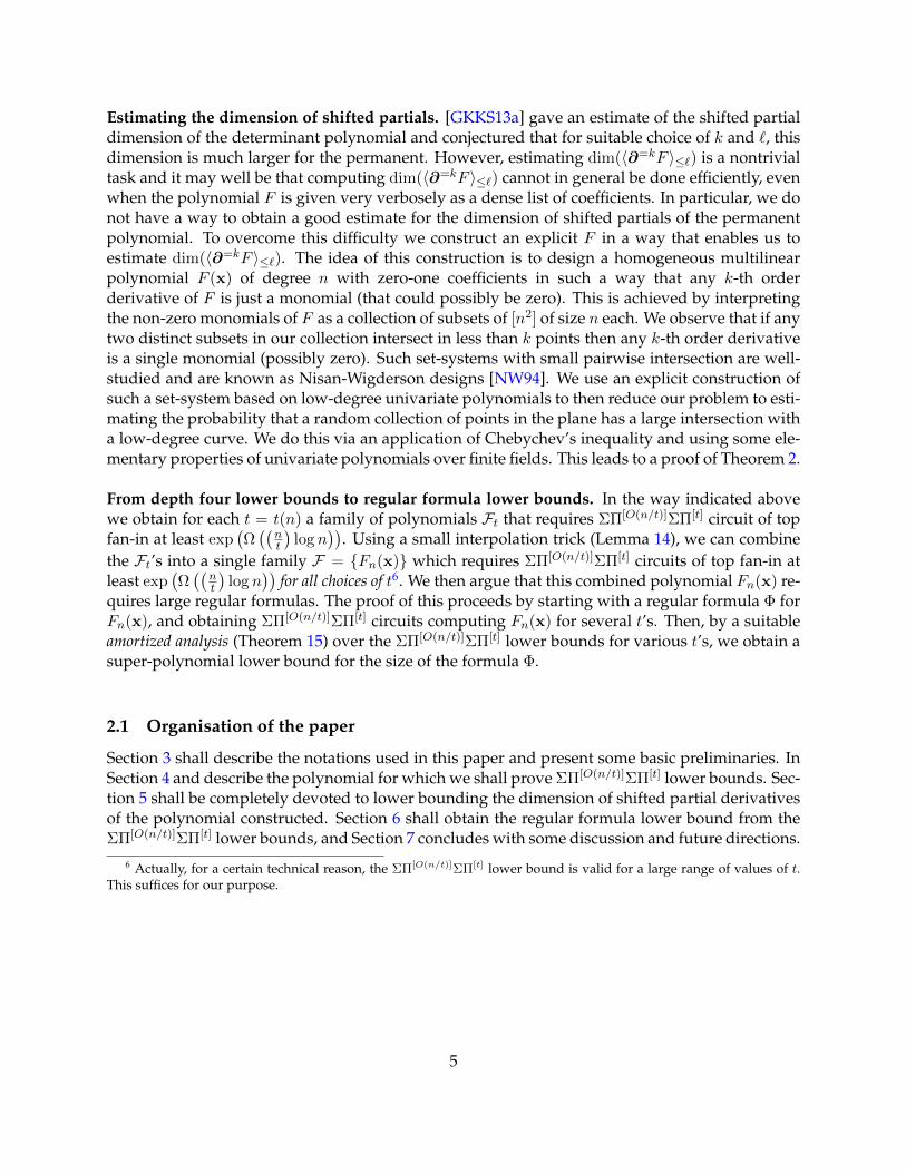
Estimating the dimension of shifted partials. [GKKS13a] gave an estimate of the shifted partialdimension of the determinant polynomial and conjectured that for suitable choice of k and `, thisdimension is much larger for the permanent. However, estimating dim(〈∂=kF 〉≤`) is a nontrivialtask and it may well be that computing dim(〈∂=kF 〉≤`) cannot in general be done efficiently, evenwhen the polynomial F is given very verbosely as a dense list of coefficients. In particular, we donot have a way to obtain a good estimate for the dimension of shifted partials of the permanentpolynomial. To overcome this difficulty we construct an explicit F in a way that enables us toestimate dim(〈∂=kF 〉≤`). The idea of this construction is to design a homogeneous multilinearpolynomial F (x) of degree n with zero-one coefficients in such a way that any k-th orderderivative of F is just a monomial (that could possibly be zero). This is achieved by interpretingthe non-zero monomials of F as a collection of subsets of [n2] of size n each. We observe that if anytwo distinct subsets in our collection intersect in less than k points then any k-th order derivativeis a single monomial (possibly zero). Such set-systems with small pairwise intersection are well-studied and are known as Nisan-Wigderson designs [NW94]. We use an explicit construction ofsuch a set-system based on low-degree univariate polynomials to then reduce our problem to esti-mating the probability that a random collection of points in the plane has a large intersection witha low-degree curve. We do this via an application of Chebychev’s inequality and using some ele-mentary properties of univariate polynomials over finite fields. This leads to a proof of Theorem 2.
From depth four lower bounds to regular formula lower bounds. In the way indicated abovewe obtain for each t = t(n) a family of polynomials Ft that requires ΣΠ[O(n/t)]ΣΠ[t] circuit of topfan-in at least exp
(Ω((
nt
)log n
)). Using a small interpolation trick (Lemma 14), we can combine
the Ft’s into a single family F = Fn(x) which requires ΣΠ[O(n/t)]ΣΠ[t] circuits of top fan-in atleast exp
(Ω((
nt
)log n
))for all choices of t6. We then argue that this combined polynomial Fn(x) re-
quires large regular formulas. The proof of this proceeds by starting with a regular formula Φ forFn(x), and obtaining ΣΠ[O(n/t)]ΣΠ[t] circuits computing Fn(x) for several t’s. Then, by a suitableamortized analysis (Theorem 15) over the ΣΠ[O(n/t)]ΣΠ[t] lower bounds for various t’s, we obtain asuper-polynomial lower bound for the size of the formula Φ.
2.1 Organisation of the paper
Section 3 shall describe the notations used in this paper and present some basic preliminaries. InSection 4 and describe the polynomial for which we shall prove ΣΠ[O(n/t)]ΣΠ[t] lower bounds. Sec-tion 5 shall be completely devoted to lower bounding the dimension of shifted partial derivativesof the polynomial constructed. Section 6 shall obtain the regular formula lower bound from theΣΠ[O(n/t)]ΣΠ[t] lower bounds, and Section 7 concludes with some discussion and future directions.
6 Actually, for a certain technical reason, the ΣΠ[O(n/t)]ΣΠ[t] lower bound is valid for a large range of values of t.This suffices for our purpose.
5
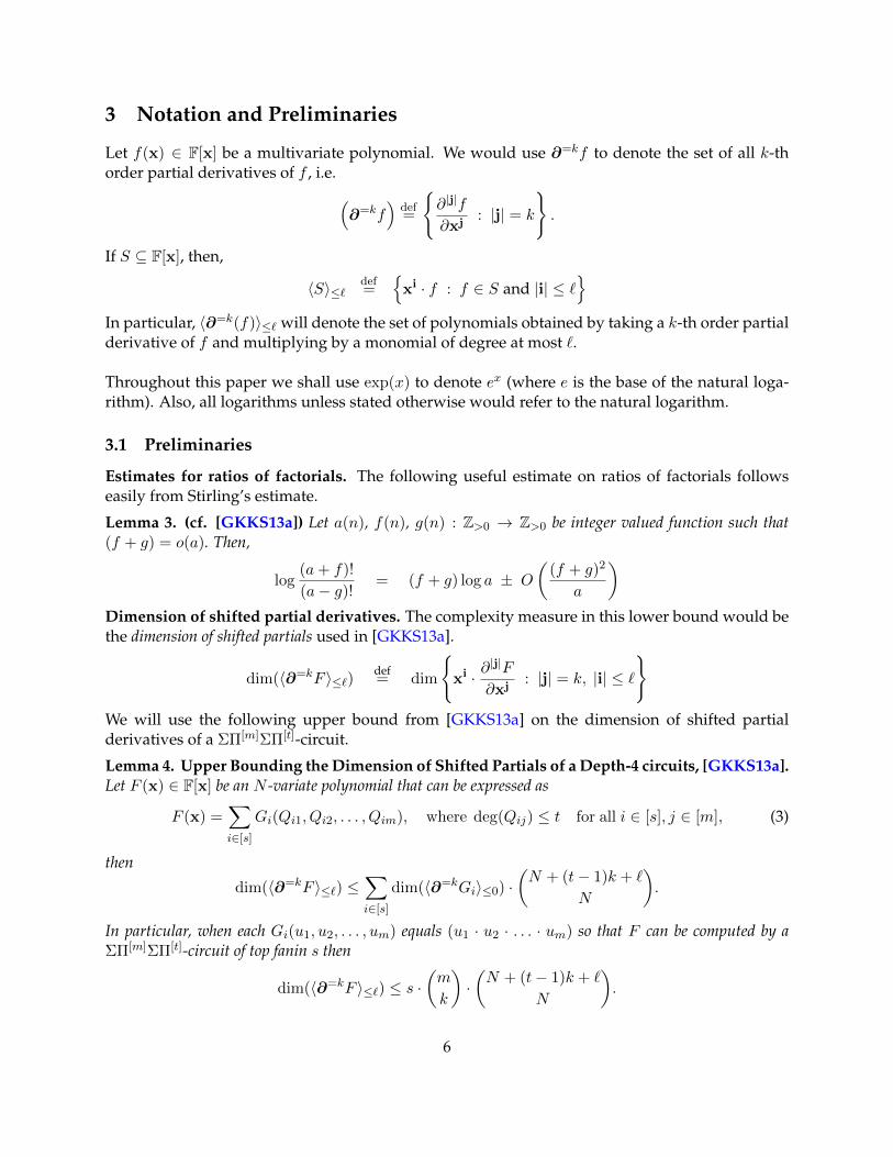
3 Notation and Preliminaries
Let f(x) ∈ F[x] be a multivariate polynomial. We would use ∂=kf to denote the set of all k-thorder partial derivatives of f , i.e. (
∂=kf)
def=
∂|j|f
∂xj: |j| = k
.
If S ⊆ F[x], then,
〈S〉≤`def=
xi · f : f ∈ S and |i| ≤ `
In particular, 〈∂=k(f)〉≤` will denote the set of polynomials obtained by taking a k-th order partialderivative of f and multiplying by a monomial of degree at most `.
Throughout this paper we shall use exp(x) to denote ex (where e is the base of the natural loga-rithm). Also, all logarithms unless stated otherwise would refer to the natural logarithm.
3.1 Preliminaries
Estimates for ratios of factorials. The following useful estimate on ratios of factorials followseasily from Stirling’s estimate.
Lemma 3. (cf. [GKKS13a]) Let a(n), f(n), g(n) : Z>0 → Z>0 be integer valued function such that(f + g) = o(a). Then,
log(a+ f)!
(a− g)!= (f + g) log a ± O
((f + g)2
a
)Dimension of shifted partial derivatives. The complexity measure in this lower bound would bethe dimension of shifted partials used in [GKKS13a].
dim(〈∂=kF 〉≤`)def= dim
xi · ∂
|j|F
∂xj: |j| = k, |i| ≤ `
We will use the following upper bound from [GKKS13a] on the dimension of shifted partialderivatives of a ΣΠ[m]ΣΠ[t]-circuit.
Lemma 4. Upper Bounding the Dimension of Shifted Partials of a Depth-4 circuits, [GKKS13a].Let F (x) ∈ F[x] be an N -variate polynomial that can be expressed as
F (x) =∑i∈[s]
Gi(Qi1, Qi2, . . . , Qim), where deg(Qij) ≤ t for all i ∈ [s], j ∈ [m], (3)
thendim(〈∂=kF 〉≤`) ≤
∑i∈[s]
dim(〈∂=kGi〉≤0) ·(N + (t− 1)k + `
N
).
In particular, when each Gi(u1, u2, . . . , um) equals (u1 · u2 · . . . · um) so that F can be computed by aΣΠ[m]ΣΠ[t]-circuit of top fanin s then
dim(〈∂=kF 〉≤`) ≤ s ·(m
k
)·(N + (t− 1)k + `
N
).
6
3.2 ABPs to regular formulas
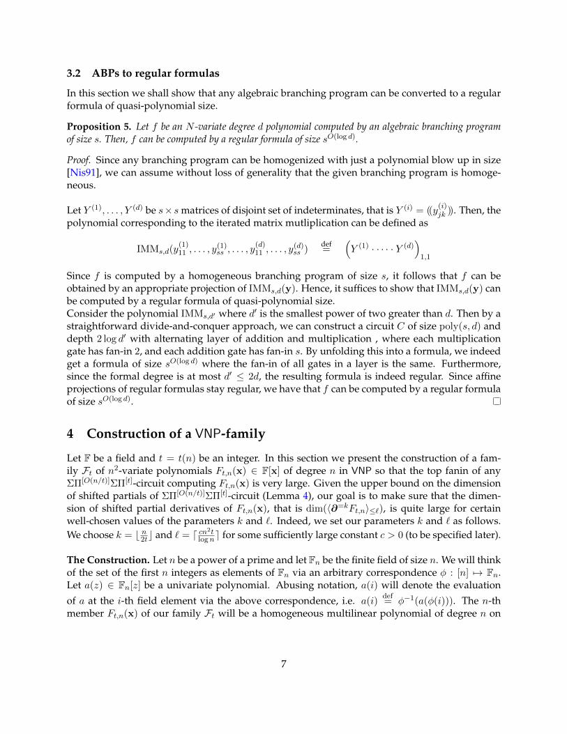
In this section we shall show that any algebraic branching program can be converted to a regularformula of quasi-polynomial size.
Proposition 5. Let f be an N -variate degree d polynomial computed by an algebraic branching programof size s. Then, f can be computed by a regular formula of size sO(log d).
Proof. Since any branching program can be homogenized with just a polynomial blow up in size[Nis91], we can assume without loss of generality that the given branching program is homoge-neous.
Let Y (1), . . . , Y (d) be s× s matrices of disjoint set of indeterminates, that is Y (i) = ((y(i)jk )). Then, the
polynomial corresponding to the iterated matrix mutliplication can be defined as
IMMs,d(y(1)11 , . . . , y
(1)ss , . . . , y
(d)11 , . . . , y
(d)ss )
def=
(Y (1) · · · · · Y (d)
)1,1
Since f is computed by a homogeneous branching program of size s, it follows that f can beobtained by an appropriate projection of IMMs,d(y). Hence, it suffices to show that IMMs,d(y) canbe computed by a regular formula of quasi-polynomial size.Consider the polynomial IMMs,d′ where d′ is the smallest power of two greater than d. Then by astraightforward divide-and-conquer approach, we can construct a circuit C of size poly(s, d) anddepth 2 log d′ with alternating layer of addition and multiplication , where each multiplicationgate has fan-in 2, and each addition gate has fan-in s. By unfolding this into a formula, we indeedget a formula of size sO(log d) where the fan-in of all gates in a layer is the same. Furthermore,since the formal degree is at most d′ ≤ 2d, the resulting formula is indeed regular. Since affineprojections of regular formulas stay regular, we have that f can be computed by a regular formulaof size sO(log d).
4 Construction of a VNP-family
Let F be a field and t = t(n) be an integer. In this section we present the construction of a fam-ily Ft of n2-variate polynomials Ft,n(x) ∈ F[x] of degree n in VNP so that the top fanin of anyΣΠ[O(n/t)]ΣΠ[t]-circuit computing Ft,n(x) is very large. Given the upper bound on the dimensionof shifted partials of ΣΠ[O(n/t)]ΣΠ[t]-circuit (Lemma 4), our goal is to make sure that the dimen-sion of shifted partial derivatives of Ft,n(x), that is dim(〈∂=kFt,n〉≤`), is quite large for certainwell-chosen values of the parameters k and `. Indeed, we set our parameters k and ` as follows.We choose k = b n2tc and ` = d cn2t
logne for some sufficiently large constant c > 0 (to be specified later).
The Construction. Let n be a power of a prime and let Fn be the finite field of size n. We will thinkof the set of the first n integers as elements of Fn via an arbitrary correspondence φ : [n] 7→ Fn.Let a(z) ∈ Fn[z] be a univariate polynomial. Abusing notation, a(i) will denote the evaluation
of a at the i-th field element via the above correspondence, i.e. a(i)def= φ−1(a(φ(i))). The n-th
member Ft,n(x) of our family Ft will be a homogeneous multilinear polynomial of degree n on
7

the n2 variables x11, x12, . . . , xnn and is defined as follows.
Ft,n(x11, . . . , xnn) =∑
a(z)∈Fn[z]deg a(z)<k
x1,a(1) · x2,a(2) · . . . · xn,a(n). (4)
To simplify the exposition, we will omit the correspondence φ and will often identify a variablexi,j by the point (φ(i), φ(j)) ∈ Fn × Fn and a monomial
(x1,a(1) · x2,a(2) · . . . · xn,a(n)
)of Ft,n(x)
with the corresponding univariate polynomial a(z) ∈ Fn[z] or the corresponding subset Sadef=
(1, a(1)), . . . , (n, a(n)) ⊆ F2n. We denote by Sk the set of all Sa’s in which the polynomial a(z) ∈
Fn[z] has degree less than k, i.e.
Skdef=Sa ⊆ F2
n : a(z) ∈ Fn[z] and deg(a) < k.
Upper bounds for the family Ft. Our construction is clearly very explicit so that the family Ft isimmediately seen to be in VNP.
Proposition 6. For any t = t(n) ≤ n, the family Ft is in the class VNP. Moreover, Ft,n(x) canbe computed by ΣΠ circuits of size 2O((n/t)·logn) (and therefore also by ΣΠ[(n/t)]ΣΠ[t]-circuits) of size2O((n/t)·logn).
Proof. Let Ft,n(x) in Ft be the polynomial of degree n as defined in equation (4). It is trivial toconstruct a polynomial time algorithm that given a monomial xe checks if the coefficient of thismonomial in Ft,n(x) is zero or one. Hence, by Valiant’s criterion [Val79, Proposition 4], Ft is inthe class VNP. Moreover, by definition, the number of monomials in Ft,n(x) equals the numberof polynomials a(z) ∈ Fn[z] of degree (k − 1). Thus Ft,n(x) has nk = 2(bn/2tc)·logn monomials andhence can be computed by ΣΠ-circuits of size 2O((n/t)·logn).
Estimating Shifted Partials via monomial counting. Now notice that since any two distinct uni-variate polynomials a(z) 6= b(z) ∈ Fn[z] of degree less than k each can agree on at most (k − 1)points therefore the size of the intersection of the corresponding image sets, |Sa ∩ Sb|, is less thank. This in turn means that any two monomials in Ft,n(x) have at most (k−1) variables in commonso that every k-th order partial derivative of Ft,n(x) is either zero or just a monomial. We thushave:
Proposition 7. Let t = t(n) be an integer and let Ft,n(x) ∈ Ft be the degree n polynomial defined inequation (4). Let k = b n2tc. Then the set of k-th order partial derivatives of Ft,n(x) are monomials of theform ∏
(i,j)∈S
xij : |S| = (n− k) and ∃Sa ∈ Sk such that S ⊂ Sa
.
This characterization of the polynomials in (∂=kFt,n) also allows us to characterize the polyno-mials in 〈∂=kFt,n〉≤`. First note that since (∂=kFt,n) consists only of monomials therefore so does〈∂=kFt,n〉≤`. Note that every monomial m ∈ 〈∂=kFt,n〉≤` of support S ⊆ Fn × Fn has degree atmost (`+ n− k) and is divisible by some monomial in (∂=kFt,n). Hence, S contains a subset S′a of
8
size (n− k) of some Sa ∈ Sk. Conversely, suppose that S contains a subset S′a ⊆ Sa of size (n− k).Then, m can also be obtained by differentiating Ft,n(x) with respect to the variables Sa \ S′a toobtain
∏(i,j)∈S′a xij , and then shifted appropriately to get m. Hence we have:
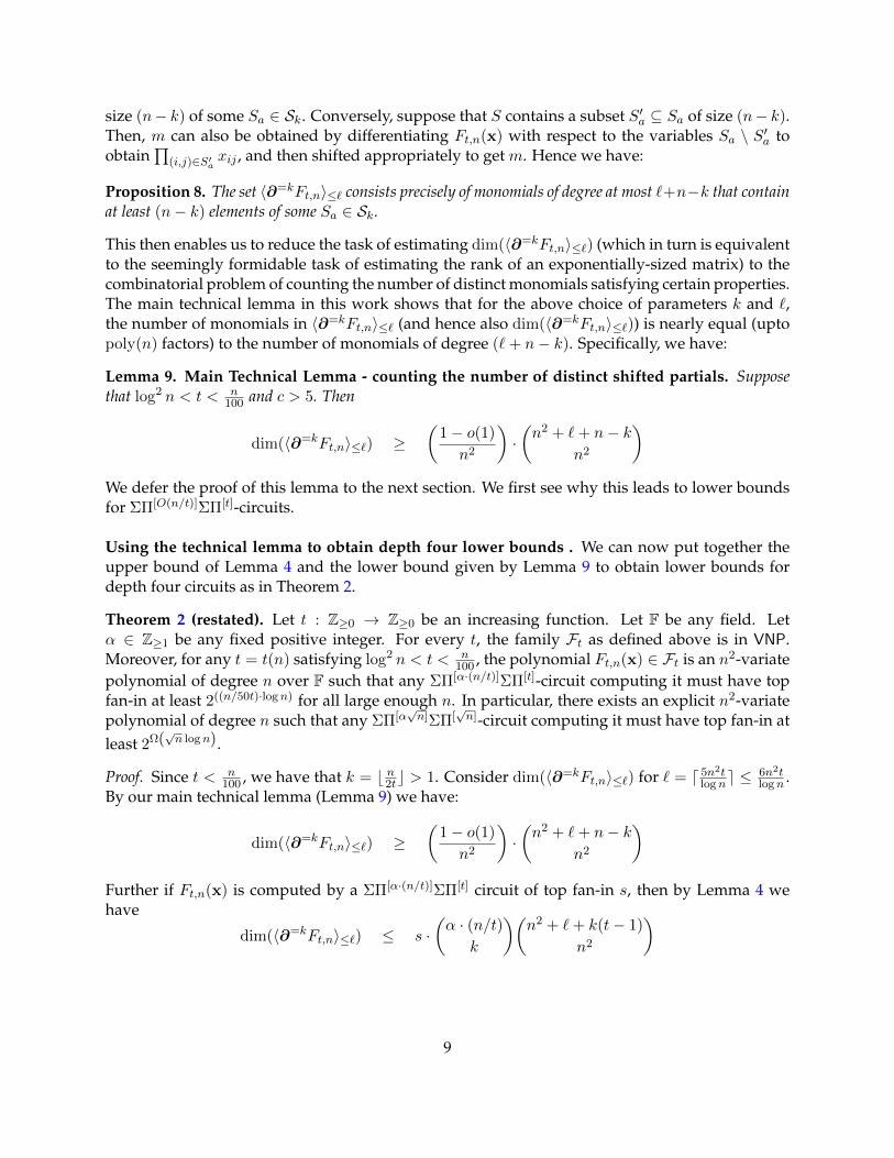
Proposition 8. The set 〈∂=kFt,n〉≤` consists precisely of monomials of degree at most `+n−k that containat least (n− k) elements of some Sa ∈ Sk.
This then enables us to reduce the task of estimating dim(〈∂=kFt,n〉≤`) (which in turn is equivalentto the seemingly formidable task of estimating the rank of an exponentially-sized matrix) to thecombinatorial problem of counting the number of distinct monomials satisfying certain properties.The main technical lemma in this work shows that for the above choice of parameters k and `,the number of monomials in 〈∂=kFt,n〉≤` (and hence also dim(〈∂=kFt,n〉≤`)) is nearly equal (uptopoly(n) factors) to the number of monomials of degree (`+ n− k). Specifically, we have:
Lemma 9. Main Technical Lemma - counting the number of distinct shifted partials. Supposethat log2 n < t < n
100 and c > 5. Then
dim(〈∂=kFt,n〉≤`) ≥(
1− o(1)
n2
)·(n2 + `+ n− k
n2
)We defer the proof of this lemma to the next section. We first see why this leads to lower boundsfor ΣΠ[O(n/t)]ΣΠ[t]-circuits.
Using the technical lemma to obtain depth four lower bounds . We can now put together theupper bound of Lemma 4 and the lower bound given by Lemma 9 to obtain lower bounds fordepth four circuits as in Theorem 2.
Theorem 2 (restated). Let t : Z≥0 → Z≥0 be an increasing function. Let F be any field. Letα ∈ Z≥1 be any fixed positive integer. For every t, the family Ft as defined above is in VNP.Moreover, for any t = t(n) satisfying log2 n < t < n
100 , the polynomial Ft,n(x) ∈ Ft is an n2-variatepolynomial of degree n over F such that any ΣΠ[α·(n/t)]ΣΠ[t]-circuit computing it must have topfan-in at least 2((n/50t)·logn) for all large enough n. In particular, there exists an explicit n2-variatepolynomial of degree n such that any ΣΠ[α
√n]ΣΠ[
√n]-circuit computing it must have top fan-in at
least 2Ω(√n logn).
Proof. Since t < n100 , we have that k = b n2tc > 1. Consider dim(〈∂=kFt,n〉≤`) for ` = d 5n2t
logne ≤6n2tlogn .
By our main technical lemma (Lemma 9) we have:
dim(〈∂=kFt,n〉≤`) ≥(
1− o(1)
n2
)·(n2 + `+ n− k
n2
)Further if Ft,n(x) is computed by a ΣΠ[α·(n/t)]ΣΠ[t] circuit of top fan-in s, then by Lemma 4 wehave
dim(〈∂=kFt,n〉≤`) ≤ s ·(α · (n/t)
k
)(n2 + `+ k(t− 1)
n2
)
9

Hence
s ≥(1− o(1)) ·
(n2+`+n−k
n2
)n2 ·
(α·(n/t)k
)(n2+`+k(t−1)n2
)=
(n2+`+n−k
n2
)(n2+`+k(t−1)n2
) · exp(−O
(nt
))· exp (−2 log n)
≥(
1 +n2
`
)(n−tk)
· exp(−O
(nt
))· exp (−2 log n) (Using Lemma 3)
≥ exp
(n2(n− tk)
2`
)· exp
(−O
(nt
))· exp (−2 log n) (Using 1 + x > ex/2 for 0 ≤ x ≤ 1)
≥ exp(( n
24t
)log n− 2 log n
)· exp
(−O
(nt
))> exp
(( n
50t
)log n
)for any log2 n < t <
n
100and sufficiently large n
5 Proof of the main technical lemma
In this section we use the characterization of 〈∂=kFt,n〉≤` given in Proposition 8 to obtain a proofof Lemma 9 and thereby obtain a lower bound on dim(〈∂=kFt,n〉≤`). Throughout the rest of thissection, the choice of the integer parameters k and ` will be as in Section 4, namely
k =⌊ n
2t
⌋and ` =
⌈5n2t
log n
⌉.
From Proposition 8 we have that 〈∂=kFt,n〉≤` consists precisely of monomials m of degree at most` + n − k that contain at least (n − k) elements of some Sa ∈ Sk. Since this condition is com-pletely determined by the support of the monomial m, it would be useful to have an estimate ofthe support size of a random monomial of degree at most `+ n− k.
Lemma 10. Most likely support size for monomials of a given degree. At least a 1n2 fraction of all
monomials of degree at most `′ = (`+ n− k) over n2 variables has support size Nmaxdef=⌊n2`′−1n2+`′+2
⌋+ 1.
Proof. The number of monomials of degree at most `′ of support size s is precisely
Nsdef=
(n2
s
)·(s+ (`′ − s)
s
)=
(n2
s
)·(`′
s
)To find out where Ns is maximised, consider the ratio of Ns+1 and Ns
Ns+1
Ns=
(n2
s+1
)·(`′
s+1
)(n2
s
)·(`′
s
) =(n2 − s)(`′ − s)
(s+ 1)2
Hence,Ns+1 > Ns if and only if (n2−s)(`′−s) > (s+1)2, which happens if and only if s < n2`′−1n2+`′+2
.
Hence, Ns increases until s =⌊n2`′−1n2+`′+2
⌋+ 1, and decreases from then on. Hence, Ns is maximised
at Nmax =⌊n2`′−1n2+`′+2
⌋+ 1.
10

Hence, for ` = d cn2tlogne, at least an 1
n2 fraction of all degree at most (` + n − k) monomials over n2
variables have support
Nmaxdef=
⌊n2`′ − 1
n2 + `′ + 2
⌋+ 1 = n2 −O
(n2 log n
t
).
That is, (n2
Nmax
)·(`+ n− kNmax
)≥ 1
n2·(n2 + `+ n− k
n2
).
Reducing to a probability estimation. We will now focus our attention on monomials m of sup-port exactly Nmax and degree at most (` + n − k). From the fact that the membership of m in〈∂=kFt,n〉≤` is completely determined by its support and using the correspondence between sup-ports of monomials and subsets of points in F2
n (Section 4), we see that our problem reduces toestimating the fraction of subsets of points in F2
n satisfying certain conditions.
Lemma 11. Let `′ = `+ n− k and let
s∗ = n2 −Nmax = n2 −⌊
n2`′ − 1
n2 + `′ + 2
⌋− 1
Let p be the probability that a random set T ⊂ F2n of size s∗ intersects one of the Sa’s in Sk in at most k
places. Then
dim(〈∂=kFt,n〉≤`) ≥ 1
n2· p ·
(n2 + `+ n− k
n2
)Proof. Let p be the fraction of monomials of degree at most `′ = (`+n−k) over n2 variables havingsupport size exactly Nmax which are in 〈∂=kFt,n〉≤`. Then from Lemma 10 we have
dim(〈∂=kFt,n〉≤`) ≥1
n2· p ·
(n2 + `+ n− k
n2
).
Now let m be a monomial of degree at most `′ and support size Nmax. We interpret the support ofm as a subset S of F2
n via the correspondence in Section 4. Then by Proposition 8 we have that mis in 〈∂=kFt,n〉≤` if and only if there exists an Sa ∈ Sk such that |S ∩ Sa| ≥ (n− k). Let T = F2
n \ S.Since every Sa ∈ Sk is of size exactly n we see that m is in 〈∂=kFt,n〉≤` if and only |T ∩ Sa| ≤ k.Finally since the number of monomials having support S depends only on the size of S we have
p = PrT⊂F2
n|T |=s∗
[|T ∩ Sa| ≤ k for some Sa ∈ Sk] ,
as required.
In this way, our task reduces to estimating p, the probability that a subset of F2n of size s∗ inter-
sects the image of a degree k polynomial in at most k places. The rest of this section is devoted toshowing that for our choice of parameters k and `, this probability p is close to one.
11
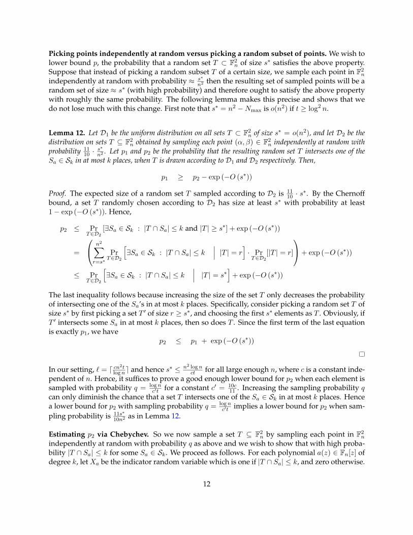
Picking points independently at random versus picking a random subset of points. We wish tolower bound p, the probability that a random set T ⊂ F2
n of size s∗ satisfies the above property.Suppose that instead of picking a random subset T of a certain size, we sample each point in F2
n
independently at random with probability ≈ s∗
n2 then the resulting set of sampled points will be arandom set of size ≈ s∗ (with high probability) and therefore ought to satisfy the above propertywith roughly the same probability. The following lemma makes this precise and shows that wedo not lose much with this change. First note that s∗ = n2 −Nmax is o(n2) if t ≥ log2 n.
Lemma 12. Let D1 be the uniform distribution on all sets T ⊂ F2n of size s∗ = o(n2), and let D2 be the
distribution on sets T ⊆ F2n obtained by sampling each point (α, β) ∈ F2
n independently at random withprobability 11
10 ·s∗
n2 . Let p1 and p2 be the probability that the resulting random set T intersects one of theSa ∈ Sk in at most k places, when T is drawn according to D1 and D2 respectively. Then,
p1 ≥ p2 − exp (−O (s∗))
Proof. The expected size of a random set T sampled according to D2 is 1110 · s
∗. By the Chernoffbound, a set T randomly chosen according to D2 has size at least s∗ with probability at least1− exp (−O (s∗)). Hence,
p2 ≤ PrT∈D2
[∃Sa ∈ Sk : |T ∩ Sa| ≤ k and |T | ≥ s∗] + exp (−O (s∗))
=
n2∑r=s∗
PrT∈D2
[∃Sa ∈ Sk : |T ∩ Sa| ≤ k
∣∣∣ |T | = r]· PrT∈D2
[|T | = r]
+ exp (−O (s∗))
≤ PrT∈D2
[∃Sa ∈ Sk : |T ∩ Sa| ≤ k
∣∣∣ |T | = s∗]
+ exp (−O (s∗))
The last inequality follows because increasing the size of the set T only decreases the probabilityof intersecting one of the Sa’s in at most k places. Specifically, consider picking a random set T ofsize s∗ by first picking a set T ′ of size r ≥ s∗, and choosing the first s∗ elements as T . Obviously, ifT ′ intersects some Sa in at most k places, then so does T . Since the first term of the last equationis exactly p1, we have
p2 ≤ p1 + exp (−O (s∗))
In our setting, ` = d cn2tlogne and hence s∗ ≤ n2 logn
ct for all large enough n, where c is a constant inde-pendent of n. Hence, it suffices to prove a good enough lower bound for p2 when each element issampled with probability q = logn
c′t for a constant c′ = 10c11 . Increasing the sampling probability q
can only diminish the chance that a set T intersects one of the Sa ∈ Sk in at most k places. Hencea lower bound for p2 with sampling probability q = logn
c′t implies a lower bound for p2 when sam-pling probability is 11s∗
10n2 as in Lemma 12.
Estimating p2 via Chebychev. So we now sample a set T ⊆ F2n by sampling each point in F2
n
independently at random with probability q as above and we wish to show that with high proba-bility |T ∩ Sa| ≤ k for some Sa ∈ Sk. We proceed as follows. For each polynomial a(z) ∈ Fn[z] ofdegree k, let Xa be the indicator random variable which is one if |T ∩ Sa| ≤ k, and zero otherwise.
12
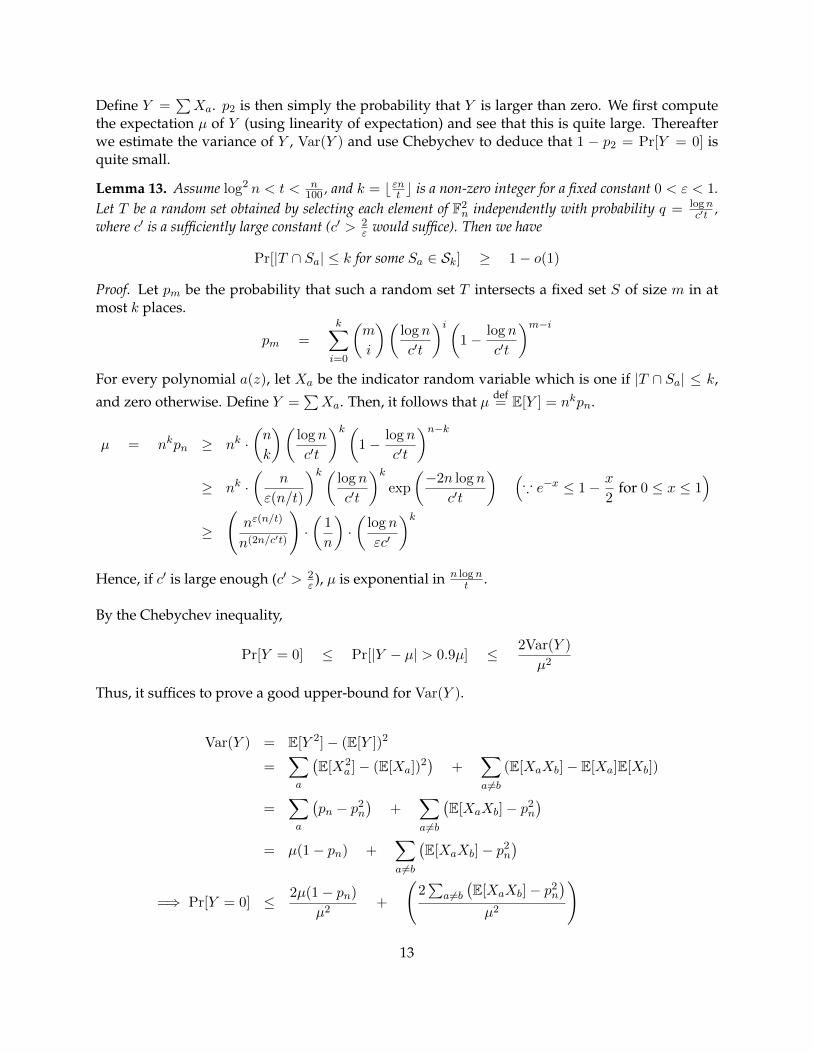
Define Y =∑Xa. p2 is then simply the probability that Y is larger than zero. We first compute
the expectation µ of Y (using linearity of expectation) and see that this is quite large. Thereafterwe estimate the variance of Y , Var(Y ) and use Chebychev to deduce that 1 − p2 = Pr[Y = 0] isquite small.
Lemma 13. Assume log2 n < t < n100 , and k = b εnt c is a non-zero integer for a fixed constant 0 < ε < 1.
Let T be a random set obtained by selecting each element of F2n independently with probability q = logn
c′t ,where c′ is a sufficiently large constant (c′ > 2
ε would suffice). Then we have
Pr[|T ∩ Sa| ≤ k for some Sa ∈ Sk] ≥ 1− o(1)
Proof. Let pm be the probability that such a random set T intersects a fixed set S of size m in atmost k places.
pm =k∑i=0
(m
i
)(log n
c′t
)i(1− log n
c′t
)m−iFor every polynomial a(z), let Xa be the indicator random variable which is one if |T ∩ Sa| ≤ k,
and zero otherwise. Define Y =∑Xa. Then, it follows that µ def
= E[Y ] = nkpn.
µ = nkpn ≥ nk ·(n
k
)(log n
c′t
)k (1− log n
c′t
)n−k≥ nk ·
(n
ε(n/t)
)k ( log n
c′t
)kexp
(−2n log n
c′t
) (∵ e−x ≤ 1− x
2for 0 ≤ x ≤ 1
)≥
(nε(n/t)
n(2n/c′t)
)·(
1
n
)·(
log n
εc′
)kHence, if c′ is large enough (c′ > 2
ε ), µ is exponential in n lognt .
By the Chebychev inequality,
Pr[Y = 0] ≤ Pr[|Y − µ| > 0.9µ] ≤ 2Var(Y )
µ2
Thus, it suffices to prove a good upper-bound for Var(Y ).
Var(Y ) = E[Y 2]− (E[Y ])2
=∑a
(E[X2
a ]− (E[Xa])2)
+∑a6=b
(E[XaXb]− E[Xa]E[Xb])
=∑a
(pn − p2
n
)+
∑a6=b
(E[XaXb]− p2
n
)= µ(1− pn) +
∑a6=b
(E[XaXb]− p2
n
)=⇒ Pr[Y = 0] ≤ 2µ(1− pn)
µ2+
(2∑
a6=b(E[XaXb]− p2
n
)µ2
)
13
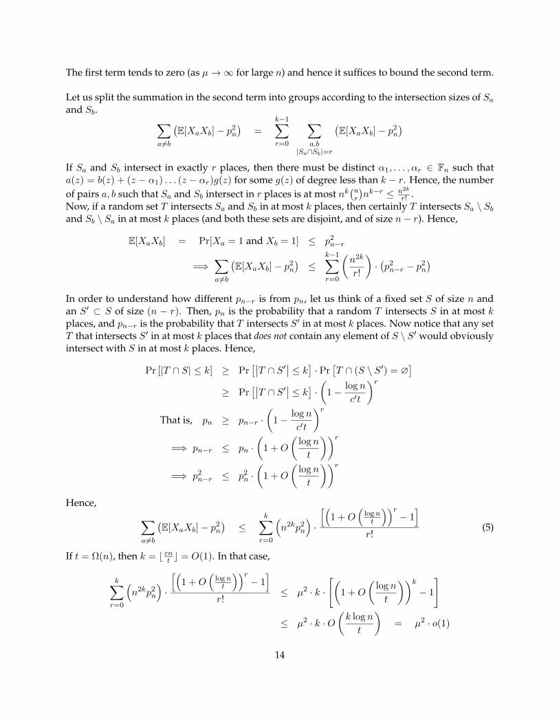
The first term tends to zero (as µ→∞ for large n) and hence it suffices to bound the second term.
Let us split the summation in the second term into groups according to the intersection sizes of Saand Sb. ∑
a6=b
(E[XaXb]− p2
n
)=
k−1∑r=0
∑a,b
|Sa∩Sb|=r
(E[XaXb]− p2
n
)If Sa and Sb intersect in exactly r places, then there must be distinct α1, . . . , αr ∈ Fn such thata(z) = b(z) + (z − α1) . . . (z − αr)g(z) for some g(z) of degree less than k − r. Hence, the numberof pairs a, b such that Sa and Sb intersect in r places is at most nk
(nr
)nk−r ≤ n2k
r! .Now, if a random set T intersects Sa and Sb in at most k places, then certainly T intersects Sa \ Sband Sb \ Sa in at most k places (and both these sets are disjoint, and of size n− r). Hence,
E[XaXb] = Pr[Xa = 1 and Xb = 1] ≤ p2n−r
=⇒∑a6=b
(E[XaXb]− p2
n
)≤
k−1∑r=0
(n2k
r!
)·(p2n−r − p2
n
)In order to understand how different pn−r is from pn, let us think of a fixed set S of size n andan S′ ⊂ S of size (n − r). Then, pn is the probability that a random T intersects S in at most kplaces, and pn−r is the probability that T intersects S′ in at most k places. Now notice that any setT that intersects S′ in at most k places that does not contain any element of S \ S′ would obviouslyintersect with S in at most k places. Hence,
Pr [|T ∩ S| ≤ k] ≥ Pr[∣∣T ∩ S′∣∣ ≤ k] · Pr
[T ∩ (S \ S′) = ∅
]≥ Pr
[∣∣T ∩ S′∣∣ ≤ k] · (1− log n
c′t
)rThat is, pn ≥ pn−r ·
(1− log n
c′t
)r=⇒ pn−r ≤ pn ·
(1 +O
(log n
t
))r=⇒ p2
n−r ≤ p2n ·(
1 +O
(log n
t
))rHence, ∑
a6=b
(E[XaXb]− p2
n
)≤
k∑r=0
(n2kp2
n
)·
[(1 +O
(lognt
))r− 1]
r!(5)
If t = Ω(n), then k = b εnt c = O(1). In that case,
k∑r=0
(n2kp2
n
)·
[(1 +O
(lognt
))r− 1]
r!≤ µ2 · k ·
[(1 +O
(log n
t
))k− 1
]
≤ µ2 · k ·O(k log n
t
)= µ2 · o(1)
14
On the other hand, if t = o(n) then k = ω(1) so that we get from (5),
∑a6=b
(E[XaXb]− p2
n
)≤ µ2 ·
∞∑r=0
(1 +O
(lognt
))rr!
−k∑r=0
1
r!
≤ µ2 ·
(e1+O( log n
t ) − e + O
(1
k!
))= µ2 · o(1) since t > log2 n and k = ω(1).
Therefore,
Var(Y ) ≤ µ(1− pn) + µ2 · o(1)
Pr[Y = 0] ≤ 2Var(Y )
µ2≤ 2
µ+ o(1) = o(1)
which tends to zero as n tends to infinity. Therefore, p2 the probability T would intersect some Sain at most k places is quite high (1− o(1)).
Lemma 9 now follows immediately from the last two lemmas.
6 Lower bound for regular formulas
In this section we will show how the lower bound for ΣΠ[O(n/t)]ΣΠ[t]-circuits leads to lowerbounds for regular formulas introduced in Section 1. From Section 5, for each log2 n < t < n
100 ,we have a construction of a family of polynomials Ft = Ft,n(x) which is exp((n/t) · log n)-hardfor the class of ΣΠ[O(n/t)]ΣΠ[t]-circuits. We first show that these different families can be com-bined using a simple interpolation trick to get a single family of polynomials F = Fn which isexp((n/t) · log n)-hard for ΣΠ[O(n/t)]ΣΠ[t]-circuits for all log2 n < t < n
100 . We will then prove aregular formula lower bound for this family by doing an ammortized analysis over the differentways of converting a regular formula into a ΣΠ[O(n/t)]ΣΠ[t]-circuit.
6.1 Combining multiple families into a single family.
Lemma 14. Let Fn(x11, . . . , xnn, u) be the (n2 + 1)-variate degree 2n polynomial defined as
Fn(x11, . . . , xnn, u) =n∑k=1
uk · Ft,n(x11, . . . , xnn)
Then, F = Fn : n ≥ 1 ∈ VNP and for every log2 n < t < n100 , any ΣΠ[O(n/t)]ΣΠ[t] circuit computing
Fn must have top fan-in at least exp(0.01
(nt
)log n
)for all large enough n.
Proof. It is clear that F is in VNP since each Ft = Ft,n is in VNP. As for the lower bound, assumeon the contrary that there is some log2 n < t < n
100 such that Fn can be computed by ΣΠ[O(n/t)]ΣΠ[t]
circuits of top fan-in exp(0.01
(nt
)log n
).
15

For every distinct7 scalars α1, . . . , αn ∈ F, and for every t ∈ [n] there exists scalars βt,1, . . . βt,n suchthat
Ft,n(x11, . . . , xnn) =
n∑i=1
βt,i · Fn(x11, . . . , xnn, αi)
In particular we then have that Ft,n can be computed by a ΣΠ[O(n/t)]ΣΠ[t] circuit C of top fan-in n · exp
(0.01
(nt
)log n
), which is at most exp
(0.02
(nt
)log n
)for any log2 n < t < n
100 . Sincesubstituting u = αi can only decrease the formal degree (which was 2n originally), the resultingcircuit continues to stay a ΣΠ[O(n/t)]ΣΠ[t] circuit computing Ft,n. But such a statement contradictsthe lower bound of Theorem 2.
Remark. This trick can be applied more generally in situations where we have families of polynomialsF1,F2, . . . ,Fr where the i-th family Fi is si(n)-hard for a subclass of circuits Ci. If every circuit subclassis subprojective (i.e. computing f(α, x2, . . . , xn) is no harder than computing f(x1, x2, . . . , xn)) and sub-additive (i.e. complexity of f(x) + g(x) is at most the sum of the complexities of f and g), then we canconstruct in the above manner a single family F which is simultaneously si(n)
r -hard for each circuit classCi.
6.2 From regular depth four circuits to regular formulas.
Theorem 15. Let F (x1, . . . , xN ) be a polynomial of degree d with the property that there exists a δ > 0such that for every log2 d < t < d
100 , any ΣΠ[O(d/t)]ΣΠ[t] circuit computing the polynomial F has topfan-in at least exp
(δ(dt
)logN
). Then, any regular formula computing F must be of size NΩ(log d).
Proof. Let Φ be a Σ[a1]Π[p1]Σ[a2]Π[p2] . . .Σ[a∆]Π[p∆]Σ[a∆+1]-regular formula computing F , whose for-mal degree
∏pi ≤ 2d.
For any i, let Ci be the depth-4 circuit obtained by converting the top 2i layers into a ΣΠ circuit,and the remaining layers by ΣΠ circuits. Since the formal degree of all polynomials at the (2i+ 1)-th layer is ti = pi+1 . . . p∆, we have that Ci is a ΣΠ[O(d/ti)]ΣΠ[ti]-circuit. Further, the top fan-in ofthe circuit Ci is upper-bounded by a1 · ap1
2 . . . ap1...pi−1
i . Hence if log2 d < ti <d
100 , applying thelower bound for ΣΠ[O(d/ti)]ΣΠ[ti] computing F , we have
a1 · ap12 . . . a
p1...pi−1
i ≥ exp
(δ
(d
ti
)logN
)Using ti = pi+1 . . . p∆ and p1 . . . p∆ ≤ 2d, we get
a1 · ap12 . . . a
p1...pi−1
i ≥ exp[(p1 . . . pi
2
)· (δ logN)
](Eqni)
Let ` be the smallest index8 with p`+1 . . . p∆ < d100 , and let h be the largest index with ph+1 . . . p∆ >
log2 d.
7If F is too small, then we can choose these scalars from a large enough extension field. Of course, any lower boundfor the extension field would continue to hold over the smaller base field.
8As a convention, let pi . . . pj = 1 if i > j. Hence, if say p∆ > d100
, we shall set ` = ∆.
16
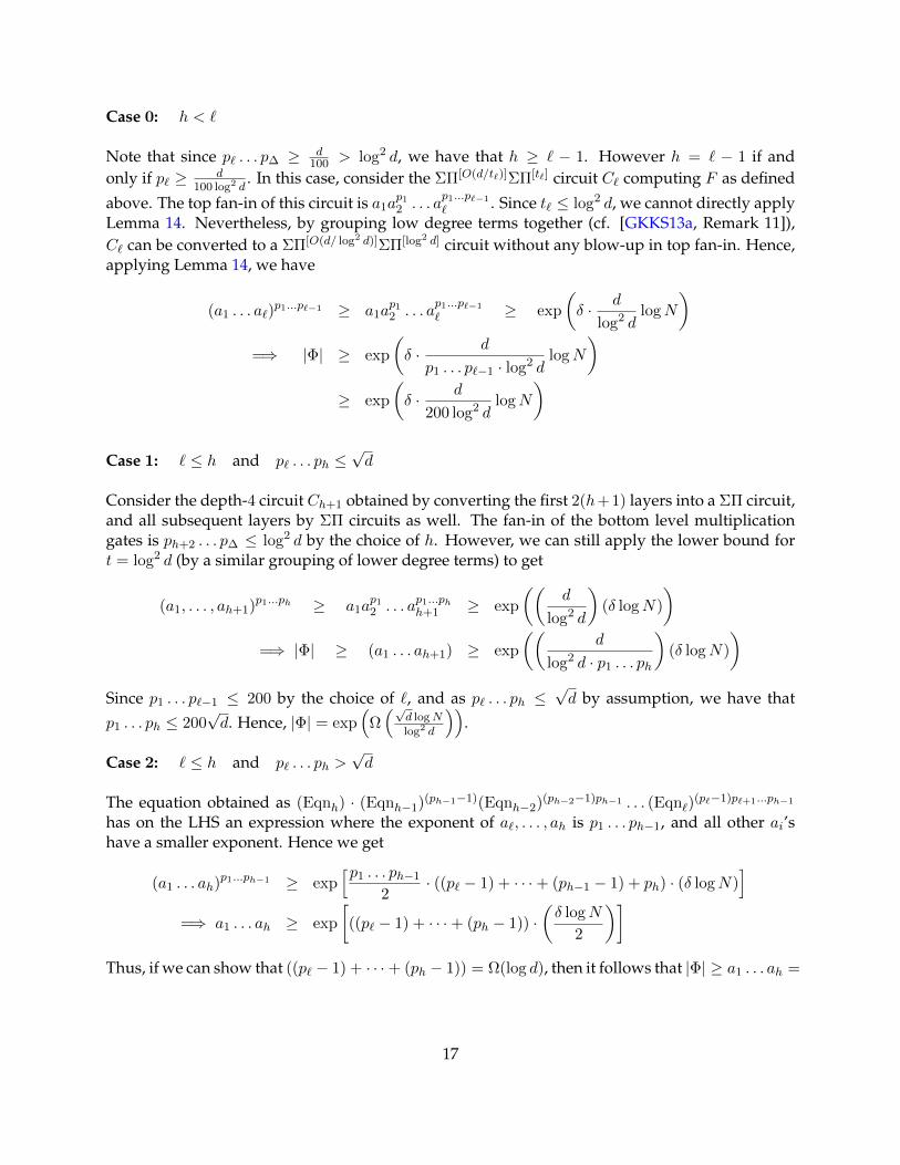
Case 0: h < `
Note that since p` . . . p∆ ≥ d100 > log2 d, we have that h ≥ ` − 1. However h = ` − 1 if and
only if p` ≥ d100 log2 d
. In this case, consider the ΣΠ[O(d/t`)]ΣΠ[t`] circuit C` computing F as defined
above. The top fan-in of this circuit is a1ap12 . . . a
p1...p`−1
` . Since t` ≤ log2 d, we cannot directly applyLemma 14. Nevertheless, by grouping low degree terms together (cf. [GKKS13a, Remark 11]),C` can be converted to a ΣΠ[O(d/ log2 d)]ΣΠ[log2 d] circuit without any blow-up in top fan-in. Hence,applying Lemma 14, we have
(a1 . . . a`)p1...p`−1 ≥ a1a
p12 . . . a
p1...p`−1
` ≥ exp
(δ · d
log2 dlogN
)=⇒ |Φ| ≥ exp
(δ · d
p1 . . . p`−1 · log2 dlogN
)≥ exp
(δ · d
200 log2 dlogN
)
Case 1: ` ≤ h and p` . . . ph ≤√d
Consider the depth-4 circuit Ch+1 obtained by converting the first 2(h+1) layers into a ΣΠ circuit,and all subsequent layers by ΣΠ circuits as well. The fan-in of the bottom level multiplicationgates is ph+2 . . . p∆ ≤ log2 d by the choice of h. However, we can still apply the lower bound fort = log2 d (by a similar grouping of lower degree terms) to get
(a1, . . . , ah+1)p1...ph ≥ a1ap12 . . . ap1...ph
h+1 ≥ exp
((d
log2 d
)(δ logN)
)=⇒ |Φ| ≥ (a1 . . . ah+1) ≥ exp
((d
log2 d · p1 . . . ph
)(δ logN)
)Since p1 . . . p`−1 ≤ 200 by the choice of `, and as p` . . . ph ≤
√d by assumption, we have that
p1 . . . ph ≤ 200√d. Hence, |Φ| = exp
(Ω(√
d logNlog2 d
)).
Case 2: ` ≤ h and p` . . . ph >√d
The equation obtained as (Eqnh) · (Eqnh−1)(ph−1−1)(Eqnh−2)(ph−2−1)ph−1 . . . (Eqn`)(p`−1)p`+1...ph−1
has on the LHS an expression where the exponent of a`, . . . , ah is p1 . . . ph−1, and all other ai’shave a smaller exponent. Hence we get
(a1 . . . ah)p1...ph−1 ≥ exp[p1 . . . ph−1
2· ((p` − 1) + · · ·+ (ph−1 − 1) + ph) · (δ logN)
]=⇒ a1 . . . ah ≥ exp
[((p` − 1) + · · ·+ (ph − 1)) ·
(δ logN
2
)]Thus, if we can show that ((p` − 1) + · · ·+ (ph − 1)) = Ω(log d), then it follows that |Φ| ≥ a1 . . . ah =
17
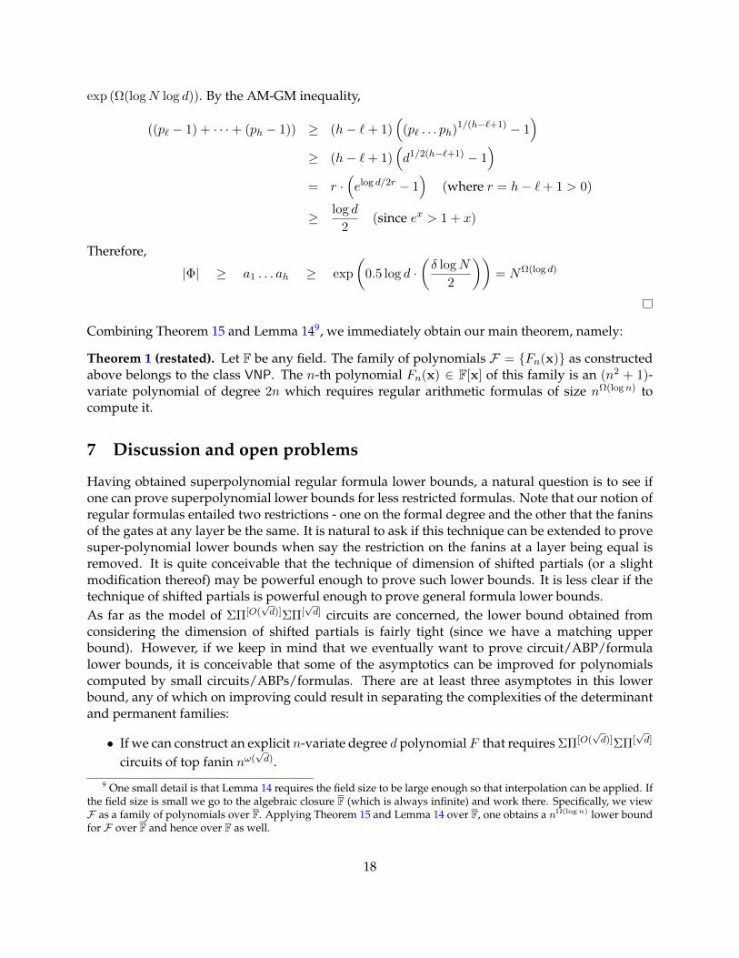
exp (Ω(logN log d)). By the AM-GM inequality,
((p` − 1) + · · ·+ (ph − 1)) ≥ (h− `+ 1)(
(p` . . . ph)1/(h−`+1) − 1)
≥ (h− `+ 1)(d1/2(h−`+1) − 1
)= r ·
(elog d/2r − 1
)(where r = h− `+ 1 > 0)
≥ log d
2(since ex > 1 + x)
Therefore,
|Φ| ≥ a1 . . . ah ≥ exp
(0.5 log d ·
(δ logN
2
))= NΩ(log d)
Combining Theorem 15 and Lemma 149, we immediately obtain our main theorem, namely:
Theorem 1 (restated). Let F be any field. The family of polynomials F = Fn(x) as constructedabove belongs to the class VNP. The n-th polynomial Fn(x) ∈ F[x] of this family is an (n2 + 1)-variate polynomial of degree 2n which requires regular arithmetic formulas of size nΩ(logn) tocompute it.
7 Discussion and open problems
Having obtained superpolynomial regular formula lower bounds, a natural question is to see ifone can prove superpolynomial lower bounds for less restricted formulas. Note that our notion ofregular formulas entailed two restrictions - one on the formal degree and the other that the faninsof the gates at any layer be the same. It is natural to ask if this technique can be extended to provesuper-polynomial lower bounds when say the restriction on the fanins at a layer being equal isremoved. It is quite conceivable that the technique of dimension of shifted partials (or a slightmodification thereof) may be powerful enough to prove such lower bounds. It is less clear if thetechnique of shifted partials is powerful enough to prove general formula lower bounds.As far as the model of ΣΠ[O(
√d)]ΣΠ[
√d] circuits are concerned, the lower bound obtained from
considering the dimension of shifted partials is fairly tight (since we have a matching upperbound). However, if we keep in mind that we eventually want to prove circuit/ABP/formulalower bounds, it is conceivable that some of the asymptotics can be improved for polynomialscomputed by small circuits/ABPs/formulas. There are at least three asymptotes in this lowerbound, any of which on improving could result in separating the complexities of the determinantand permanent families:
• If we can construct an explicit n-variate degree d polynomial F that requires ΣΠ[O(√d)]ΣΠ[
√d]
circuits of top fanin nω(√d).
9 One small detail is that Lemma 14 requires the field size to be large enough so that interpolation can be applied. Ifthe field size is small we go to the algebraic closure F (which is always infinite) and work there. Specifically, we viewF as a family of polynomials over F. Applying Theorem 15 and Lemma 14 over F, one obtains a nΩ(log n) lower boundfor F over F and hence over F as well.
18

• If we can show that any n-variate degree d polynomial F that can be computed by a polynomialsized circuit satisfies
dim(〈∂=kF 〉≤`) ≤(√
d
k
)(n+ `+ (
√d− 1)k
n
)· exp(−ω(
√d log n))
for k = ε√d and ` = cn
√d
logn .
• If we can show that any n-variate degree d polynomial that can be computed by a polynomialsized ABP can be computed by a regular formula of size no(log d).
Needless to say, a new complexity measure other than the dimension of shifted partials would bevery enlightening, and possibly is even necessary for stronger lower bounds. Nevertheless, ourlower bounds having come so close and given the recent progress in depth reduction [GKKS13b,Tav13] and lower bounds, one cannot help but be optimistic that the resolution of VP vs VNP maynot be too distant in the future.
Acknowledgements
The authors would like to thank Ankit Gupta and Pritish Kamath for many discussions, especiallyfor discussions pertaining to the power and limitations of the method of shifted partials and thechoice of a candidate hard polynomial.
References
[AV08] Manindra Agrawal and V. Vinay. Arithmetic circuits: A chasm at depth four. In FOCS,pages 67–75, 2008.
[AW09] S. Aaronson and A. Wigderson. Algebrization: A new barrier in complexity theory.ACM Transactions on Computation Theory, 1(1):1–54, 2009.
[BGS75] T. Baker, J. Gill, and R. Solovay. Relativizations of the P =? NP question. SIAM Journalon Computing, 4(4):431–442, 1975.
[BS83] W. Baur and V. Strassen. The complexity of partial derivatives. Theoretical ComputerScience, 22(3):317–330, 1983.
[GK98] Dima Grigoriev and Marek Karpinski. An exponential lower bound for depth 3 arith-metic circuits. In STOC, pages 577–582, 1998.
[GKKS13a] Ankit Gupta, Neeraj Kayal, Pritish Kamath, and Ramprasad Saptharishi. Approach-ing the chasm at depth four. In Conference on Computational Complexity (CCC), 2013.
[GKKS13b] Ankit Gupta, Neeraj Kayal, Pritish Kamath, and Ramprasad Saptharishi. Arithmeticcircuits: A chasm at depth three. Technical report, Electronic Colloquium on Compu-tational Complexity (ECCC), 2013.
[GKQ13] Ankit Gupta, Neeraj Kayal, and Youming Qiao. Random arithmetic formulas can bereconstructed efficiently. In Conference on Computational Complexity (CCC), 2013.
19

[GR00] Dima Grigoriev and Alexander A. Razborov. Exponential lower bounds for depth 3arithmetic circuits in algebras of functions over finite fields. Appl. Algebra Eng. Com-mun. Comput., 10(6):465–487, 2000.
[Kal85] K. Kalorkoti. A lower bound for the formula size of rational functions. SIAM journalof Computing, 14(3):678–687, 1985.
[Kay12] Neeraj Kayal. An exponential lower bound for the sum of powers of bounded degreepolynomials. Technical report, Electronic Colloquium on Computational Complexity(ECCC), 2012.
[Koi12] Pascal Koiran. Arithmetic circuits: The chasm at depth four gets wider. TheoreticalComputer Science, 448:56–65, 2012.
[KS13] Mrinal Kumar and Shubhangi Saraf. Lower Bounds for Depth 4 Homogeneous Cir-cuits with Bounded Top Fanin. Technical report, Electronic Colloquium on Computa-tional Complexity (ECCC), 2013.
[Nis91] Noam Nisan. Lower bounds for non-commutative computation (extended abstract).In STOC, pages 410–418, 1991.
[NW94] Noam Nisan and Avi Wigderson. Hardness vs randomness. J. Comput. Syst. Sci.,49(2):149–167, 1994.
[NW97] N. Nisan and A. Wigderson. Lower bounds on arithmetic circuits via partial deriva-tives. Computational Complexity, 6(3):217–234, 1997.
[Raz09] R. Raz. Multi-linear formulas for permanent and determinant are of super-polynomial size. Journal of the Association for Computing Machinery, 56(2), 2009.
[Raz10] Ran Raz. Tensor-rank and lower bounds for arithmetic formulas. In STOC, pages659–666, 2010.
[RR94] A.A. Razborov and S. Rudich. Natural proofs. Journal of Computer and System Sciences,55:204–213, 1994.
[RY08] R. Raz and A. Yehudayoff. Lower bounds and separations for constant depth mu-tilinear circuits. In Proceedings of the 23rd IEEE Annual Conference on ComputationalComplexity, pages 128–139, 2008.
[Rys63] H. J. Ryser. Combinatorial mathematics. Math. Assoc. of America, 14, 1963.
[SW01] A. Shpilka and A. Wigderson. Depth-3 arithmetic circuits over fields of characteristiczero. Computational Complexity, 10(1):1–27, 2001.
[SY10] Amir Shpilka and Amir Yehudayoff. Arithmetic circuits: A survey of recent resultsand open questions. Foundations and Trends in Theoretical Computer Science, 5:207–388,March 2010.
[Tav13] Sebastien Tavenas. Improved bounds for reduction to depth 4 and 3. In MathematicalFoundations of Computer Science (MFCS), 2013.
20
[Val79] Leslie G. Valiant. Completeness Classes in Algebra. In STOC, pages 249–261, 1979.
[VSBR83] L.G. Valiant, S. Skyum, S. Berkowitz, and C. Rackoff. Fast parallel computation ofpolynomials using few processors. SIAM Journal on Computing, 12(4):641–644, 1983.
21