a survey of control allocation methods for underwater vehicles · underwater vehicles . 110 problem...

7

A Survey of Control Allocation Methods for Underwater Vehicles

Thor I. Fossen1,2, Tor Arne Johansen1 and Tristan Perez3

1Dept. of Eng. Cybernetics, Norwegian Univ. of Science and Techn. 2Centre for Ships and Ocean Structures, Norwegian Univ. of Science and Techn.

3Centre of Excellence for Complex Dyn. Syst. and Control, Univ. of Newcastle, 1,2Norway 3Australia

1. Introduction A control allocation system implements a function that maps the desired control forces generated by the vehicle motion controller into the commands of the different actuators. In order to achieve high reliability with respect to sensor failure, most underwater vehicles have more force-producing actuators than the necessary number required for nominal operations. Therefore, it is common to consider the motion control problem in terms of generalised forces—independent forces affecting the different degrees of freedom—, and use a control allocation system. Then, for example, in case of an actuator failure the remaining ones can be reconfigured by the control allocation system without having to change the motion controller structure and tuning. The control allocation function hardly ever has a close form solution; instead the values of the actuator commands are obtained by solving a constrained optimization problem at each sampling period of the digital motion control implementation loop. The optimization problem aims at producing the demanded generalized forces while at the same time minimizing the use of control effort (power). Control allocation problems for underwater vehicles can be formulated as optimization problems, where the objective typically is to produce the specified generalized forces while minimizing the use of control effort (or power) subject to actuator rate and position constraints, power constraints as well as other operational constraints. In addition, singularity avoidance for vessels with rotatable thrusters represents a challenging problem since a non-convex nonlinear program must be solved. This is useful to avoid temporarily loss of controllability. In this article, a survey of control allocation methods for over-actuated underwater vehicles is presented. The methods are applicable for both surface vessels and underwater vehicles. Over-actuated control allocation problems are naturally formulated as optimization problems as one usually wants to take advantage of all available degrees of freedom (DOF) in order to minimize power consumption, drag, tear/wear and other costs related to the use of control, subject to constraints such as actuator position limitations, e.g. Enns (1998), Bodson (2002) and Durham (1993). In general, this leads to a constrained optimization

saa046

Text Box

Licensed under the Creative Commons Attribution-NonCommercial-ShareAlike 3.0 license. http://creativecommons.org/licenses/by-nc-sa/3.0/

Underwater Vehicles

110

problem that is hard to solve using state-of-the-art iterative numerical optimization software at a high sampling rate in a safety-critical real-time system with limiting processing capacity and high demands for software reliability. Still, real-time iterative optimization solutions can be used; see Lindfors (1993), Webster and Sousa (1999), Bodson (2002), Harkegård (2002) and Johansen, Fossen, Berge (2004). Explicit solutions can also be found and implemented efficiently by combining simple matrix computations, logic and filtering; see Sørdalen (1997), Berge and Fossen (1997) and Lindegaard and Fossen (2003).

Fig. 1. Block diagram illustrating the control allocation problem.

The paper presents a survey of control allocation methods with focus on mathematical representation and solvability of thruster allocation problems. The paper is useful for university students and engineers who want to get an overview of state-of-the art control allocation methods as well as advance methods to solve more complex problems.

1.1 Problem formulation Consider an underwater vehicle (Fossen, 2002):

=η η ν

ν + ν ν + ν ν + η = τJ

M C D g( )

( ) ( ) ( ) (1.1)

that is controlled by designing a feedback control law of generalized control forces:

nτ = α ∈B u R( ) (1.2)

where pα∈R is a vector azimuth angles and r∈u R are actuator commands. For marine vehicles, some control forces can be rotated an angle about the z-axis and produce force components in the x- and y-directions, or about the y-axis and produce force components in the x- and z-directions. This gives additional control inputsα which must be computed by the control allocation algorithm. The control law uses feedback from position/attitude

Tx y z ϕ θ ψ=η [ , , , , , ] and velocity Tu v w p q r=ν [ , , , , , ] as shown in Figure 1. For marine vessels with controlled motion in n DOF it is necessary to distribute the generalized control forces τ to the actuators in terms of control inputsα and u. Consider (1.2) where n r×α ∈B R( ) is the input matrix. If B has full rank (equal to n) and r n> , you have control forces in all relevant directions, this is an over-actuated control problem. Similarly, the case r n< is referred to as an under-actuated control problem. Computation of α andu from τ is a model-based optimization problem which in its simplest form is unconstrained while physical limitations like input amplitude and rate saturations imply that a constrained optimization problem must be solved. Another complication is actuators that can be rotated at the same time as they produce control forces. This increases the number of available controls from r to r+p.


111

2. Actuator models The control force due to a propeller, a rudder, or a fin can be written

F ku= (1.3)

where k is the force coefficient and u is the control input depending on the actuator considered; see Table 1. The linear model F=ku can also be used to describe nonlinear monotonic control forces. For instance, if the rudder force F is quadratic in rudder angle δ, that is

δ δ= | |,F k (1.4) the choice | |u δ δ= , which has a unique inverse ( )sign u uδ = , satisfies (1.3).

Actuator u α Tf Main propeller/longitudinal thrusters

pitch/rpm - [ ,0,0]xF

Transverse thrusters pitch/rpm - [0, ,0]yF

Rotatable thruster in the horizontal plane

pitch/rpm angle α α[ , ,0]cos sinx xF F

Rotatable thruster in the vertical plane

pitch/rpm angle α α[ sin ,0, cos ]z zF F

Aft rudders angle - [0, ,0]yF

Stabilizing fins angle - [0,0, ]zF

Table 1. Example of actuators and control variables.

For underwater vehicles the most common actuators are: • Main propellers/longitudinal thrusters are mounted aft of the hull usually in

conjunction with rudders. They produce the necessary force in the x-direction needed for transit.

• Transverse thrusters are sometime going through the hull of the vessel (tunnel thrusters). The propeller unit is then mounted inside a transverse tube and it produces a force in the y -direction. Tunnel thrusters are only effective at low speed which limits their use to low-speed maneuvering and DP.

• Rotatable (azimuth) thrusters in the horizontal and vertical planes are thruster units that can be rotated an angleα about the z-axis or y-axis to produce two force components in the horizontal or vertical planes, respectively. Azimuth thrusters are attractive in low-speed maneuvering and DP systems since they can produce forces in different directions leading to an over-actuated control problem that can be optimized with respect to power and possible failure situations.

• Aft rudders are the primary steering device for conventional vessels. They are located aft of the vessel and the rudder force yF will be a function of the rudder deflection (the

Underwater Vehicles

112

drag force in the x-direction is usually neglected in the control analysis). A rudder force in the y-direction will produce a yaw moment which can be used for steering control.

• Stabilizing fins are used for damping of vertical vibrations and roll motions. They produce a force zF in the z-directions which is a function of the fin deflection. For small angles this relationship is linear. Fin stabilizers can be retractable allowing for selective use in bad weather. The lift forces are small at low speed so the most effective operating condition is in transit.

• Control surfaces can be mounted at different locations to produce lift and drag forces. For underwater vehicles these could be fins for diving, rolling, and pitching, rudders for steering, etc.

Table 1 implies that the forces and moments in 6 DOF due to the force vector [ , , ]x z

TyF F Ff = can be written

x

y

z

z y y z

x z z x

y x x y

FFF

F l F lF l F lF l F l

⎡ ⎤⎢ ⎥⎢ ⎥⎢ ⎥⎡ ⎤ ⎢ ⎥= =⎢ ⎥ ⎢ ⎥×⎣ ⎦ ⎢ ⎥⎢ ⎥⎢ ⎥⎣ ⎦

−−−

fr f

τ

(1.5)

where [ , , ]x zT

yl l lr = are the moment arms. For azimuth thrusters in the horizontal plane the control force F will be a function of the rotation angle. Consequently, an azimuth thruster will have two force components cosxF F α= and sin ,yF F α= while the main propeller aft of the vehicle only produces a longitudinal force ,xF F= see Table 1.

2.1 Thrust configuration matrix for non-rotatable actuators The control forces and moments for the fixed thruster case (no rotatable thrusters) can be written

τ = Tf (1.6) where n r×∈T R is the thrust configuration matrix. The control forces satisfies,

,=f Ku (1.7) with control inputs 1 ,..., ][ .T

ruu=u The force coefficient matrix r r×∈K R is diagonal,

1{ ,..., }.rdiag k k=K (1.8) The actuator configuration matrix is defined in terms of a set of column vectors

ni ∈t R according to

1( ) [ ,..., ].rα =T t t (1.9)

If we consider 6 DOF motions, the columns vectors can be derived from (1.5) and (1.9) according to


113

⎡ ⎤⎡ ⎤ ⎡ ⎤⎢ ⎥⎢ ⎥ ⎢ ⎥⎢ ⎥⎢ ⎥ ⎢ ⎥⎢ ⎥⎢ ⎥ ⎢ ⎥⎢ ⎥⎢ ⎥ ⎢ ⎥= = =−⎢ ⎥⎢ ⎥ ⎢ ⎥⎢ ⎥⎢ ⎥ ⎢ ⎥−⎢ ⎥⎢ ⎥ ⎢ ⎥⎢ ⎥⎢ ⎥ ⎢ ⎥⎣ ⎦⎣ ⎦ ⎣ ⎦tunnel thruster stabilizing finmain propeller and aft rudder

0

01 010 000 1

0

0

i i

i

i i

i i iz y

z x

y x

l

l lll l

t t t (1.10)

2.2 Thrust configuration matrix for rotatable actuators A more general representation of (1.6) is,

( )( ) ,

τ = αα

T f= T Ku

(1.11)

where the thrust configuration matrix )( n r×∈T Rα varies with the azimuth angles

1[ ,..., ] .Tpα αα =

(1.12)

The azimuth thruster in the horizontal plane are defined in terms of the column vector

α

α

ααα

ααα α

α α α

⎡ ⎤⎡ ⎤⎢ ⎥⎢ ⎥⎢ ⎥⎢ ⎥⎢ ⎥⎢ ⎥⎢ ⎥⎢ ⎥= =− ⎢ ⎥⎢ ⎥⎢ ⎥⎢ ⎥ −⎢ ⎥⎢ ⎥⎢ ⎥⎢ ⎥−⎣ ⎦ ⎣ ⎦−

azimuth thruster in azthe horizontal plane

sincos0sin

cos0, cossin

sin sin cossin cos sin

ii

i i i

i i i

ii

i

ii i y iz i

z i z i x i

x i y i y i

l l l

ll

l l l

t t

imuth thruster inthe vertical plane

(1.13)

where the coordinates ( , , )i i ix y zl l l denotes the location of the actuator with respect the body

fixed coordinate system. Similar expressions can be derived for thrusters that are rotatable about the x- and y-axes.

2.3 Extended thrust configuration matrix for rotatable actuators When solving the control allocation optimization problem an alternative representation to (1.10) is attractive to use. Equation (1.11) is nonlinear in the controls α and u. This implies that a nonlinear optimization problem must be solved. In order to avoid this, the rotatable thrusters can be treated as two forces. Consider a rotatable thruster in the horizontal plane (the same methodology can be used for thrusters that can be rotated in the vertical plane),

= cos

cos ,

F Fx i ik ui i i

iα

α=

(1.14)

Underwater Vehicles

114

= sin

sin .

F Fy i ik ui i i

iα

α= (1.15)

Next, we define an extended force vector according to

e e e=f K u (1.16) such that

e e eτ = TK u (1.17)

where eT and eK are the extended thrust configuration and thrust coefficient matrices, respectively and eu is a vector of extended control inputs where the azimuth controls are modelled as

cossin

ix i i

iy i i

u uu u

αα

==

(1.18)

The following examples show how this model can be established for an underwater vehicle equipped with two main propellers and two azimuth thrusters in the horizontal plane. Example 1: Thrust configuration matrices for an ROV/AUV with rotatable thrusters The horizontal plane forces X and Y in surge and sway, respectively and the yaw moment N satisfy (see Figure 2),

( )T Kuτ = α (1.19)

1 1 2 2 3 4

1 1

2 2

3 31 1 2 2

4 4

0 0 01 0 1 1

0 0 00 1 0 0 .

0 0 0sin cos sin cos

0 0 0x y x y y y

k uX

k uY

k uN l l l l l l

k uα α α α

⎡ ⎤ ⎡ ⎤⎡ ⎤⎡ ⎤ ⎢ ⎥ ⎢ ⎥⎢ ⎥⎢ ⎥ ⎢ ⎥ ⎢ ⎥= ⎢ ⎥⎢ ⎥ ⎢ ⎥ ⎢ ⎥⎢ ⎥⎢ ⎥ − − ⎢ ⎥ ⎢ ⎥⎣ ⎦ ⎣ ⎦ ⎢ ⎥ ⎢ ⎥⎣ ⎦ ⎣ ⎦

(1.20)

Fig. 2. ROV/AUV equipped with two azimuth thrusters (forces F1 and F2) and two main propellers (forces F3 and F4). The azimuth forces are decomposed along the x- and y-axis.


115

By using the extended thrust vector, (1.19) can be rewritten as,

e e eT K uτ = (1.21)

1 2 3 4

1111

22

22

3 34 4

0 0 0 0 00 0 0 0 0

1 0 1 0 1 10 0 0 0 0

0 1 0 1 0 0 .0 0 0 0 0

0 00 0 0 0 00 0 0 0 0

x

y

x

yx x y y

ukuk

Xuk

Yuk

N l l l lk u

k u

⎡ ⎤⎡ ⎤⎢ ⎥⎢ ⎥⎢ ⎥⎢ ⎥⎡ ⎤⎡ ⎤ ⎢ ⎥⎢ ⎥⎢ ⎥⎢ ⎥ ⎢ ⎥= ⎢ ⎥⎢ ⎥⎢ ⎥ ⎢ ⎥⎢ ⎥⎢ ⎥⎢ ⎥ − ⎢ ⎥⎣ ⎦ ⎢ ⎥⎣ ⎦⎢ ⎥⎢ ⎥⎢ ⎥⎢ ⎥⎣ ⎦ ⎣ ⎦

(1.22)

Notice that eT is constant while ( )T α depends on .α This means that the extended control input vector eu can be solved directly from (1.21) by using a pseudo-inverse. This is not the case for (1.20) which represents a nonlinear optimization problem. The azimuth controls can then be derived from the extended control vector eu by mapping the pairs 1 1( , )x yu u and 2 2( , )x yu u using the relations,

2 21 1 1 1 1

2

1

22 2 2 2 22

, atan 2( , ),

, atan 2( , ).

x y y x

x y y x

u u u u u

u u u u u

α

α

= + =

= + = (1.23)

The last two controls u3 and u4 are elements in ue. □

3. Linear quadratic unconstrained control allocation The simplest allocation problem is the one where all control forces are produced by thrusters in fixed directions alone or in combination with rudders and control surfaces such that

constant, ( ) constant.= = =T Tα α Assume that the allocation problem is unconstrained-i.e., there are no bounds on the vector elements ,i if α and iu and their time derivatives. Saturating control and constrained control allocation are discussed in Sections 4-5. For marine craft where the configuration matrix T is square or non-square ( )r n≥ , that is there are equal or more control inputs than controllable DOF, it is possible to find an optimal distribution of control forces f, for each DOF by using an explicit method. Consider the unconstrained least-squares (LS) optimization problem (Fossen & Sagatun, 1991),

{ }subject to:

min

TJ =

− =f

f Wf

Tf 0.τ (1.24)

Here W is a positive definite matrix, usually diagonal, weighting the control forces. For marine craft which have both control surfaces and propellers, the elements in W should be

Underwater Vehicles

116

selected such that using the control surfaces is much more inexpensive than using the propellers.

3.1 Explicit solution forα = constant using lagrange multipliers Define the Lagrangian (Fossen, 2002),

( , ) ( ),T TL = + −f f Wf Tfλ λ τ (1.25) where r∈Rλ is a vector of Lagrange multipliers. Consequently, differentiating the Lagrangian L with respect to ,f yields

112

2T TL −∂

= − = =∂

Wf T 0 f W Tf

λ ⇒ λ. (1.26)

Next, assume that 1 T−TW T is non-singular such that

1 1 11 2( )

2T T− − −= = =τ λ ⇒ λ τ.Tf TW T TW T

(1.27) This gives

− −= 1 12( ) ,Tλ τTW T (1.28)

Substituting (1.28) into (1.27) yields,

1 1 1† †, ( ) ,T T

w w− − −= =τf T T W T TW T (1.29)

where †wT is recognized as the generalized inverse. For the case W=I, that is equally weighted

control forces, (1.29) reduces to the Moore-Penrose pseudo inverse,

1† ) .T T −=T T (TT (1.30)

Since † ,w=f T τ the control input vector u can be computed from (1.7) as,

1 †

w−= τ.u K T (1.31)

Notice that this solution is valid for all α but not optimal with respect to a time-varying α.

3.2 Explicit solution for varyingα using Lagrange multipliers In the unconstraint case a time-varying α can be handled by using an extended thrust representation similar to Sørdalen (1997). Consider the ROV/AUV model in Example 1 where,

e e

e e e

τ = T f= T K u

(1.32)

Application of (1.29) now gives,


117

†

1 ,e w

e e e−

= τ

=

f T

u K f (1.33)

where 1 1 2 2 3 4[ , , , , , ]Te x y x yu u u u u u=u and 1 2 3 4 5 6[ , , , , , ] .Te f f f f f f=f The optimal azimuth

angles and thrust commands are then found as

2 2 2 21 1 1 1 2 1 1

1

2 2 2 22 2 2 3 4 2 2

2

53

3

64

4

1

2

1 , atan 2( , ),

1 , atan 2( , ),

,

.

x y y x

x y y x

u u u f f u uk

u u u f f u uk

fukfuk

α

α

= + = + =

= + = + =

=

=

(1.34)

The main problem is that the optimal solution for 1α and 2α can jump at each sample which requires proper filtering. In the next sections, we propose other solutions to this problem.

4. Linear quadratic constrained control allocation In practical systems it is important to minimize the power consumption by taking advantage of the additional control forces in an over-actuated control problem. It is also important to take into account actuator limitations like saturation, tear and wear as well as other constraints such as forbidden sectors, and overload of the power system. In general this leads to a constrained optimization problem.

4.1 Explicit solution forα = constant using piecewise linear functions (non-rotatable actuators) An explicit solution approach for parametric quadratic programming has been developed by Tøndel et al. (2003) while applications to marine vessels are presented by Johansen et al. (2005). In this work the constrained optimization problem is formulated as

{ }, ,

min max

1 2

min

, ,...

subject to:

T T

f

r

J f

f f f f f

β=

= +≤

− ≤ ≤

f sf Wf s Qs

Tf sf f f

+ +

τ≤

(1.35)

where ns ∈ R is a vector of slack variables and forces

1 2[ , ,..., ] RT rrf f f= ∈f (1.36)

Underwater Vehicles

118

The first term of the criterion corresponds to the LS criterion (1.25), while the third term is introduced to minimize the largest force max | |i if f= among the actuators. The constant

0β ≥ controls the relative weighting of the two criteria. This formulation ensures that the constraints min max

i i if f f≤ ≤ ( 1,..., )i r= are satisfied, if necessary by allowing the resulting generalized force Tf to deviate from its specification τ . To achieve accurate generalized force, the slack variable should be close to zero. This is obtained by choosing the weighting matrix 0.>Q W Moreover, saturation and other constraints are handled in an optimal manner by minimizing the combined criterion (1.35). Let

2 1

min max[ , , , ] R ,T T T T n rβ + +∈p f f= τ (1.37) denote the parameter vector and,

1[ , , ] R .T T T r nf + +∈z f s= (1.38)

Hence, it is straightforward to see that the optimization problem (1.35) can be reformulated as a QP problem:

{ }

1 1

2 2

subject to:

min

T TJ =

=

Φ +

≤

zz z z Rp

A z C pA z C p

(1.39)

where:

1( ) 1

1 ( 1) ( 2 )

1 1

: , :1

0

r n rr n

n r n r n n r

r n

× ×+ ×

× × + + × +

× ×

⎡ ⎤⎡ ⎡ ⎤ ⎤⎢ ⎥

= = ⎢ ⎢ ⎥ ⎥⎢ ⎥⎢ ⎢ ⎥ ⎥⎣ ⎣ ⎦ ⎦⎢ ⎥

⎣ ⎦

ΦW 0 0

00 Q 0 R 00 0

1

1

1 1 2,, :

11

111

1

r r r n r

r r r n r

r r r n

n n n

r r r n

× × ×

× × ×

× ×

× ×

× ×

−⎡ ⎤⎢ ⎥⎢ ⎥⎢ ⎥⎡ ⎤⎢ ⎥⎢ ⎥⎢ ⎥⎢ ⎥⎢ ⎥⎢ ⎥⎢ ⎥⎡ ⎤ ⎢ ⎥= − =⎣ ⎦ ⎢ ⎥⎢ ⎥⎣ ⎦⎢ ⎥⎡ ⎤⎢ ⎥⎢ ⎥⎢ ⎥⎢ ⎥⎢ ⎥− ⎢ ⎥⎢ ⎥⎢ ⎥⎢ ⎥⎢ ⎥⎣ ⎣ ⎦ ⎦

I 0 0I 0 0

I 0A T I 0 A

I 0

(1.40)

1

11 (2 1) 2

1

1

,, :

r n r r r r r

r n r r r r rn n n r

r n r r r r r

r n r r r r r

× × × ×

× × × ×× × +

× × × ×

× × × ×

−⎡ ⎤⎢ ⎥⎢ ⎥⎡ ⎤= =⎣ ⎦ ⎢ ⎥⎢ ⎥⎢ ⎥⎣ ⎦

0 I 0 00 0 I 0

C I 0 C0 0 0 00 0 0 0


119

Since 0W > and 0Q > this is a convex quadratic program in z parameterized by p. Convexity guarantees that a global solution can be found. The optimal solution ( )∗z p is a continuous piecewise linear function ( )∗z p defined on any subset,

min max≤ ≤p p p (1.41)

of the parameter space. Moreover, an exact representation of this piecewise linear function can be computed off-line using multi-parametric QP algorithms (Tøndel and Johansen, 2003b) or the Matlab Multi-Parametric Toolbox (MPT) by Kvasnica, Grieder and Baotic (2004). Consequently, it is not necessary to solve the QP (1.36) in real time for the current value of τ and the parameters min max,f f and β , if they are allowed to vary. In fact it suffices to evaluate the known piecewise linear function ( )∗z p as a function of the given parameter vector p which can be done efficient with a small amount of computations. For details on the implementation aspects of the mp-QP algorithm; see Johansen et al. (2003) and references therein. An on-line control allocation algorithm is presented in Tøndel et al. (2003a).

4.2 Explicit solution for varyingα using piecewise linear functions (rotatable thrusters and rudders) An extension of the mp-QP algorithm to marine vessels equipped with azimuthing thrusters and rudders has been given by Johansen et al. (2003). A propeller with a rudder can produce a thrust vector within a range of directions and magnitudes in the horizontal plane for low-speed maneuvering and dynamic positioning. The set of attainable thrust vectors is non-convex because significant lift can be produced by the rudder only with forward thrust. The attainable thrust region can, however, be decomposed into a finite union of convex polyhedral sets. A similar decomposition can be made for azimuthing thrusters including forbidden sectors. Hence, this can be formulated as a mixed-integer-like convex quadratic programming problem and by using arbitrarily number of rudders as well as thrusters and other propulsion devices can be handled. Actuator rate and position constraints are also taken into account. Using a multi-parametric quadratic programming software, an explicit piecewise linear representation of the least-squares optimal control allocation law can be pre-computed. The method is illustrated using a scale model of a supply vessel in a test basin, see Johansen et al. (2003) for details, and using a scale model of a floating platform in a test basin, see Spjøtvold (2008).

4.3 Explicit solutions based on minimum norm and null-space methods (non-rotatable actuators) In flight and aerospace control systems, the problems of control allocation and saturating control have been addressed by Durham (1993, 1994a, 1994b). They also propose an explicit solution to avoid saturation referred to as the direct method. By noticing that there are infinite combinations of admissible controls that generate control forces on the boundary of the closed subset of attainable controls, the direct method calculates admissible controls in the interior of the attainable forces as scaled down versions of the unique solutions for force demands. Unfortunately it is not possible to minimize the norm of the control forces on the boundary or some other constraint since the solutions on the boundary are unique. The

Underwater Vehicles

120

computational complexity of the algorithm is proportional to the square of the number of controls, which can be problematic in real-time applications. In Bordignon and Durham (1995) the null space interaction method is used to minimize the norm of the control vector when possible, and still access the attainable forces to overcome the drawbacks of the direct method. This method is also explicit but much more computational intensive. For instance 20 independent controls imply that up to 3.4 billon points have to be checked at each sample. In Durham (1999) a computationally simple and efficient method to obtain near-optimal solutions is described. The method is based on prior knowledge of the controls' effectiveness and limits such that pre-calculation of several generalized inverses can be done.

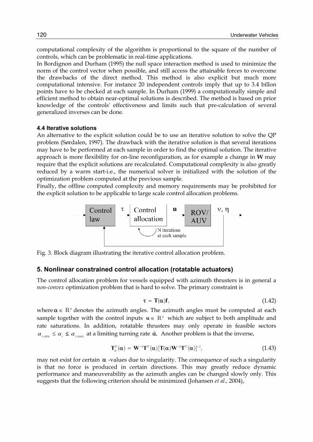
4.4 Iterative solutions An alternative to the explicit solution could be to use an iterative solution to solve the QP problem (Sørdalen, 1997). The drawback with the iterative solution is that several iterations may have to be performed at each sample in order to find the optimal solution. The iterative approach is more flexibility for on-line reconfiguration, as for example a change in W may require that the explicit solutions are recalculated. Computational complexity is also greatly reduced by a warm start-i.e., the numerical solver is initialized with the solution of the optimization problem computed at the previous sample. Finally, the offline computed complexity and memory requirements may be prohibited for the explicit solution to be applicable to large scale control allocation problems.

Fig. 3. Block diagram illustrating the iterative control allocation problem.

5. Nonlinear constrained control allocation (rotatable actuators) The control allocation problem for vessels equipped with azimuth thrusters is in general a non-convex optimization problem that is hard to solve. The primary constraint is

( ) ,= T fτ α (1.42) where Rp∈α denotes the azimuth angles. The azimuth angles must be computed at each sample together with the control inputs R p∈u which are subject to both amplitude and rate saturations. In addition, rotatable thrusters may only operate in feasible sectors

,min ,maxi i iα α α≤ ≤ at a limiting turning rate α. Another problem is that the inverse,

1 1 1( ) ( )[ ( ) ( )] ,T T T

w− − −=T W T T W Tα α α α (1.43)

may not exist for certain α -values due to singularity. The consequence of such a singularity is that no force is produced in certain directions. This may greatly reduce dynamic performance and maneuverability as the azimuth angles can be changed slowly only. This suggests that the following criterion should be minimized (Johansen et al., 2004),


121

3/2

, ,1

0 0

1 ?

min max

min max

min 0 max

min

( ) ( )

det( ( ) ( ))

( )

subject to

rT

i ii

T

J P f

ρε

=

−

⎧⎪ = +⎨⎪⎩+ − −

⎫+ ⎬

+ ⎭

+≤ ≤≤

Δ ≤

∑f ss Qs

T W T

T f sf f f

α

α α Ω α α

α α

α = τ

α α ≤ αα α − α ≤ Δα

(1.44)

where

• 3/2

1ri i iP f=∑ represents power consumption where 0 ( 1,..., )iP i r> = are positive

weights. • Ts Qs penalizes the error sbetween the commanded and achieved generalized force.

This is necessary in order to guarantee that the optimization problem has a feasible solution for any τ and 0.α The weight 0Q > is chosen so large that the optimal solution is s 0≈ whenever possible.

• min max≤ ≤f f f is used to limit the use of force (saturation handling).

• min max≤α α ≤ α denotes the feasible sectors of the azimuth angles.

• min 0 maxΔ ≤α α − α ≤ Δα ensures that the azimuth angles do not move to much within

one sample taking 0α equal to the angles at the previous sample. This is equivalent to limiting | |,α -i.e. the turning rate of the thrusters.

• The term

1det( ( ) ( ))T

ρε −+ T W Tα α

is introduced to avoid singular configurations given by 1det( ( ) ( )) 0.T− =T W Tα α To avoid division by zero, 0,ε > is chosen as a small number, while 0ρ > is scalar weight. A large ρ ensures high maneuverability at the cost of higher power consumption and vice versa.

The optimization problem (1.44) is a non-convex nonlinear program and it requires a significant amount of computations at each sample (Nocedal and Wright, 1999). Consequently, the following two implementation strategies are attractive alternatives to nonlinear program efforts.

5.1 Dynamic solution using Lyapunov methods In Johansen (2004) a control-Lyapunov approach has been used to develop an optimal dynamic control allocation algorithm. The proposed algorithm leads to asymptotic optimality. Consequently, the computational complexity compared to a direct nonlinear programming approach is considerably reduced. This is done by constructing the

Underwater Vehicles

122

optimizing control allocation algorithm as a dynamic update law which can be used together with a feedback control system. It is shown that the asymptotically optimal control allocation algorithm in interaction with an exponentially stable trajectory-tracking controller guarantees uniform boundedness and uniform global exponential convergence. A case study addressing low-speed maneuvering of an overactuated ship is used to demonstrate the performance of the control allocation algorithm. Extension to the adaptive case where thrust losses are estimated are given in (Tjønnås & Johansen, 2005), and extension to the case when actuator dynamics are considered explicitly in the control allocation is given in (Tjønnås & Johansen, 2007).

5.2 Iterative solutions using quadratic programming The problem (1.42) can be locally approximated with a convex QP problem by assuming that: 1. the power consumption can be approximated by a quadratic term in ,f near the last

force 0f such that 0 .+ Δf f f= 2. the singularity avoidance penalty can be approximated by a linear term linearized

about the last azimuth angle 0α such that 0 .= + Δα α α The resulting QP criterion is (Johansen et al. , 2004):

{

( )

0

0 0

0 0, ,

1

0 0 0,

min 0 max 0

min 0 max 0

min max

min ( ) ( )

det( ( ) ( ))

( ) ( ) ( )

subject to

T

T T

T

J

ρε

Δ

−

∂∂

= + Δ + Δ

+ + Δ Δ⎫∂ ⎛ ⎞ ⎪+ Δ ⎬⎜ ⎟∂ +⎝ ⎠ ⎪⎭

= −

− ≤ ≤ −− ≤ −

Δ ≤

f s

f

f f P f f

s Qs

T W T

s T f T f T f

f f f f f

Δα

α

α α

α Ω α

αα α α

+ α Δ + α Δα τ α

α α Δα ≤ α αα Δα ≤ Δα

(1.45)

The convex QP problem (1.43) can be solved by using standard software for numerical optimization.

5.3 Iterative solutions using linear programming Linear approximations to the thrust allocation problem have been discussed by Webster and Sousa (1999) and Lindfors (1993). In Linfors (1993) the azimuth thrust constraints

2 2 max( cos ) ( sin )i i i i i if f f fαα= + ≤ (1.46)

are represented as circles in the ( cos , sin )i i i if f αα -plane. The nonlinear program is

transformed to a linear programming (LP) problem by approximating the azimuth thrust constraints by straight lines forming a polygon. If 8 lines are used to approximate the circles (octagons), the worst case errors will be less than ± 4.0%. The criterion to be minimized is a linear combination of | |,f that is magnitude of force in the x- and y-directions, weighted against the magnitudes


123

2 2| ( cos ) ( sin ) |i i i if f αα + (1.47)

representing azimuth thrust. Hence, singularities and azimuth rate limitations are not weighted in the cost function. If these are important, the QP formulation should be used.

5.4 Explicit solution using the singular value decomposition and filtering techniques An alternative method to solve the constrained control allocation problem is to use the singular value decomposition (SVD) and a filtering scheme to control the azimuth directions such that they are aligned with the direction where most force is required, paying attention to singularities (Sørdalen 1997). Results from sea trials have been presented in Sørdalen (1997). A similar technique using the damped-least squares algorithm has been reported in Berge and Fossen (1997) where the results are documented by controlling a scale model of a supply vessel equipped with four azimuth thrusters.

6. Case study: allocation problem formulation for an AUV with control surfaces Some underwater vehicles perform all their missions at forward speed. In these applications, the vehicle hull design is streamlined so as to reduce hull drag, and the preferred type of control surface is the hydrofoil or fin. Hydrofoils produce lift, which is the useful force for controlling the motion of the vehicle. The side effect of lift generation, however, is drag—in other words, drag is the price we pay to obtain lift. Hence, for vehicles with several mounted control surfaces, the control allocation seeks the implementation of the demanded generalised forces while minimising the foil-induced drag. In this section, we formulate the control allocation problem for an AUV with two fixed thrusters and hydrofoil control surfaces. Figure 4 shows INFANTE—an AUV built and operated by the Insituto Supetior Tecnico de Lisboa, Portugal. This AUV has two fixed thrusters at the stern, and six control surfaces: two horizontal fins mounted on the bow quarter, two horizontal fins mounted on the stern quarter, and two rudders mounted vertically behind the propellers.

Fig. 4. INFANTE-AUV. Picture courtesy of Dynamic Systems and Ocean Robotics Laboratory (DSOR), Instituto Superior Tecnico de Lisboa, Portugal. Copyright (c) 2001 DSOR-ISR. Standard hydrofoil theory, see for example Marchaj (2000), establishes that the lift force produced by the hydrofoils is directed perpendicular to the incoming flow while the drag

Underwater Vehicles

124

force is directed along the incoming flow direction. The magnitude of the lift and drag forces can be modelled as,

21

,2 w f LL Au Cρ δ=

(1.48)

2 21

,2 w f DD Au Cρ δ=

(1.49)

where wρ is the water density, A is the area of the hydrofoil, uf is the fluid velocity relative to the hydrofoil, CL and CD are the lift and drag coefficients respectively (measured experimentally), and δ is the angle of attack between the hydrofoil and the incoming flow. Table 2 shows the different variables associated with the different control actuators considered in this case study. Notice that for the positive angle deflection of the control surfaces we use the right-hand rule along the direction of the rotation axis towards the tip.

Variable Description Positive convention δ pb Port bow fin angle Forward edge down δ sb Starboard bow fin angle Forward edge up δ ps Port stern fin angle Forward edge down δ ss Starboard stern fin angle Forward edge up δ pr Port rudder angle Forward edge to port δ sr Starboard rudder angle Forward edge to port Tp Port thuster thust Forward Ts Starboard thuster thust Forward

Table 2. Manipulated variables associated with the different actuators of the AUV shown in Figure 4. For the control allocation problem, we will assume that the velocity uf is either measured or estimated. We will also assume that the vehicle manoeuvres slowly from its equilibrium operational condition at forward speed. Hence, we can neglect the small drift angles; and thus, the lift and drag forces of the different hydrofoils can be considered to act along the x- and y-direction of the body-fixed coordinate system attached to the vessel. Furthermore, under the slow manoeuvring assumption and small drift angle, the angle of attack δ of the hydrofoils can be approximated by the mechanical angle of rotation of the hydrofoils. For the particular vehicle under study, we can consider motion control objectives in 5DOF (surge, heave, pitch, roll, and yaw). With these objectives, the fins can be used to control heave, pitch and roll, the rudders to control yaw, and the thrusters to control surge. Then, we can simplify the allocation problem by taking a three-step approach: 1. Solve the allocation of the fins to obtain the deflection angles that implement the

desired heave force and pitch and roll moments while minimising the induced drag. 2. Compute rudder angles based on the demanded yaw moment. 3. Compute thrust demand for the thrusters based on the demanded surge force while

compensating for the fin and rudder induced drag forces. The separation into these three steps simplifies the optimisation problem associated with the allocation. The first step results in a quadratic programme with linear constraints since only the lift forces are used. Then the rudders are used only for controlling the heading or yaw.


125

Finally, after computing the fin and rudder deflection angles, the thrust can be computed to implement the desired surge force and to compensate for the drag forces of the fins and rudders. The above allocation scheme could be interpreted as a feed-forward compensation for the side effects of the fin and rudder drag induced forces. Step 1: fin Allocation Based on the above assumptions and the adopted positive convention for the variables shown in Table 1, we obtain the following vector of fin commands and force configuration matrix for heave, pitch and roll allocation

,

T

fins pb sb ps ssδ δ δ δ⎡ ⎤= ⎣ ⎦f

(1.50)

,

b b s sL L L Lb b s s

fins pb L sb L ps L ss Lb b s s

pb L sb L ps L ss L

k k k k

x k x k x k x k

y k y k y k y k

⎡ ⎤− −⎢ ⎥

= − −⎢ ⎥⎢ ⎥− −⎣ ⎦

T

(1.51)

where

2

2

1,

21

.2

b bL w b f L

s sL w s f L

k A v C

k A v C

ρ

ρ

=

=

(1.52)

Since the fin-induced drag is proportional to the square of the angle of attack, a natural objective function to minimize in the control allocation problem is a quadratic function. Depending on the difference in size and hydrodynamic characteristics of the bow and stern hydrofoils, we could perhaps use a different weighting to the two sets of fins. Thus, the fin allocation problem can be formulated as a standard quadratic program:

{ },

subject to

,

T T

fins

min +

= −≤

≥

f sf W f s Qs

T f t sMf Ns 0

(1.53)

with

max

4 4 min

4 4 max

min

0 0 0

0 0 0, , , ,

0 0 0

0 0 0

bb

bb

ss

ss

w

w

w

w

δδδδ

×

×

⎡ ⎤⎡ ⎤⎢ ⎥⎢ ⎥ Δ⎡ ⎤ ⎡ ⎤ ⎢ ⎥⎢ ⎥= = = Δ =⎢ ⎥ ⎢ ⎥ ⎢ ⎥⎢ ⎥ − Δ⎢ ⎥ ⎢ ⎥⎣ ⎦ ⎣ ⎦ ⎢ ⎥⎢ ⎥⎢ ⎥⎢ ⎥⎣ ⎦ ⎣ ⎦

IW M N

I

(1.54)

where wb and ws represent the weighting for the bow and stern fins—note that only their relative value is of importance.

Underwater Vehicles

126

Step 2: Rudder Allocation In nominal operational conditions, we can use the same deflection for both rudders. Hence, the allocation problem reduces to inverse of the mapping from angle to rudder moment:

2

,cpr sr r

r r prop L

N

x A v Cδ δ

ρ= =

(1.55)

where xr denotes the longitudinal position of the rudders relative to the adopted body-fixed reference system, vprop is the flow velocity in the wake of the propeller, Nc is the yaw moment demanded by the vehicle motion controller. Step 3: Thruster Allocation In nominal operational conditions, we can use the same demand for the two thrusters. This demand is computed to implement the desired thrust demanded by the controller and to compensate the drag induced by the fins and rudders

( )1

,2p s c csT T X X= = +

(1.56)

where Xc is the surge force demanded by the vehicle motion controller, and Xcs is the added resistance due to the deflection of all the control surfaces

( ) ( ) ( )2 2 2 2 2 2 ,b s rcs D pb sb D ps ss D pr srX k k kδ δ δ δ δ δ= + + + + +

(1.57)

with the following drag related coefficients for the bow fins, stern fins, and rudders respectively

2

2

2

1,

21

,21

.2

b bD w b f D

s sD w s f D

r rD w r prop D

k A v C

k A v C

k A v C

ρ

ρ

ρ

=

=

=

(1.58)

In this section, we have considered a case study and formulated the control allocation problem for a particular AUV with two thrusters and six control surfaces. We have made some simplifying assumptions and considered the nominal operational conditions. Similar modelling procedures to that followed in this case study can be applied to other AUV with different actuators.

7. Conclusion A survey of methods for control allocation of overactuated marine vessels has been presented. Both implicit and explicit methods formulated as optimization problems have been discussed. The objective has been to minimize the use of control effort (or power) subject to actuator rate and position constraints, power constraints as well as other operational constraints. A case study of an AUV with control surfaces has been included in order to show how quadratic programming can be used to solve the control allocation problem.


127

8. References Berge, S. P. and T. I. Fossen (1997). Robust Control Allocation of Overactuated Ships:

Experiments With a Model Ship. Proc. of the 4th IFAC Conference on Manoeuvring and Control of Marine Craft, pp. 166-171, Brijuni, Croatia.

Bodson, M. (2002). Evaluation of Optimization Methods for Control Allocation. Journal of Guidance, Control and Dynamics, vol. 25, pp. 703-711.

Bordignon, K. A. and W. C. Durham (1995). Closed-Form Solutions to Constrained Control Allocation Problem. Journal of Guidance, Control and Dynamics, vol. 18, no. 5, pp. 1000-1007.

Durham, W. C. (1993). Constrained Control Allocation. Journal of Guidance, Control and Dynamics, vol. 16, no. 4, pp. 717-725.

Durham, W. C. (1994a). Constrained Control Allocation: Three Moment Problem. Journal of Guidance, Control and Dynamics, vol. 17, no. 2, pp. 330-336.

Durham, W. C. (1994b). Attainable Moments for the Constrained Control Allocation Problem. Journal of Guidance, Control and Dynamics, vol.17, no. 6, pp. 1371-1373.

Durham, W. C. (1999). Efficient, Near-Optimal Control Allocation. Journal of Guidance, Control and Dynamics, vol. 22, no. 2, pp. 369-372.

Enns, D. (1998). Control Allocation Approaches, Proceedings of the AIAA Guidance, Navigation, and Control Conference and Exhibit. pp. 98-108, Reston, VA.

Fossen, T. I. (1994). Guidance and Control of Ocean Vehicles. John Wiley and Sons Ltd., ISBN 0 471-94113-1.

Fossen, T. I. (2002). Marine Control Systems: Guidance, Navigation and Control of Ships, Rigs and Underwater Vehicles, Marine Cybernetics AS, ISBN 82-92356-00-2.

Fossen, T. I. and S. I. Sagatun (1991). Adaptive Control of Nonlinear Systems: A Case Study of Underwater Robotic Systems. Journal of Robotic Systems, vol. 8, no. 3, pp. 393-412.

Harkegård, O. (2002). Efficient Active Set Algorithms for Solving Constraint Least Squares Problems in Aircraft Control Allocation. Proc. of the 41st IEEE Conference on Decision and Control (CDC’02), 2002.

Johansen, T. A. (2004). Optimizing Nonlinear Control Allocation. Proc. of the IEEE Conf. Decision and Control (CDC’04), pp. 3435-3440, Nassau, Bahamas.

Johansen, T. A., T. I. Fossen and S. P. Berge (2004). Constraint Nonlinear Control Allocation with Singularity Avoidance using Sequential Quadratic Programming. IEEE Transactions on Control Systems Technology, vol. 12, pp. 211-216.

Johansen, T. A., T. I. Fossen and P. Tøndel (2005). Efficient Optimal Constrained Control Allocation via Multi-Parametric Programming. AIAA Journal of Guidance, Control and Dynamics}, vol. 28, pp. 506--515.

Johansen, T. A., T. P. Fuglseth, P. Tøndel and T. I. Fossen (2003). Optimal Constrained Control Allocation in Marine Surface Vessels with Rudders. Proc. of the IFAC Conf. Manoeuvring and Control of Marine Craft, Girona, Spain.

Kvasnica, M., P. Grieder and M. Baotic (2004). Multi-Parametric Toolbox (MPT), <http://control.ee.ethz.ch/~mpt>.

Lindegaard, K.-P. and T. I. Fossen (2002). Fuel Efficient Control Allocation for Surface Vessels with Active Rudder Usage: Experiments with a Model Ship. IEEE Transactions on Control Systems Technology, vol. 11, pp. 850-862.

Underwater Vehicles

128

Lindfors, I. (1993). Thrust Allocation Method for the Dynamic Positioning System. Proc. Of the 10th International Ship Control Systems Symposium (SCSS'93), pp. 3.93-3.106, Ottawa, Canada.

Marchaj, C. A. (2000). Aero-hydrodynamic of Sailing, 3rd Edition. Adlard Coles Publishing. ISBN 1-888671-18-1.

Nocedal, J. and S. J. Wright (1999). Numerical Optimization. Springer-Verlag, New York. Sørdalen, O. J. (1997). Optimal Thrust Allocation for Marine Vessels. Control Engineering

Practice, vol. 5, no. 9, pp. 1223-1231. Spjøtvold, J. (2008). Parametric Programming in Control Theory. PhD thesis, Norwegian

University of Science and Technology, Trondheim. Tjønnås, J., T. A. Johansen (2005). Optimizing Nonlinear Adaptive Control Allocation. Proc.

of the IFAC World Congress, Prague. Tjønnås, J., T. A. Johansen (2007). Optimizing Adaptive Control Allocation with Actuator

Dynamics. Proc. of the IEEE Conference on Decision and Control, New Orleans. Tøndel, P., T. A. Johansen and A. Bemporad (2003a). An Algorithm for Multi-parametric

Quadratic Programming and explicit MPC solutions. Automatica, vol. 39, pp. 489-497.

Tøndel, P., T. A. Johansen and A. Bemporad (2003b). Evaluation of Piecewise Affine Control via Binary Searh Tree. Automatica, vol. 39, pp. 743-749.

Webster, W. C. and J. Sousa (1999). Optimum Allocation for Multiple Thrusters. Proc. of the Int. Society of Offshore and Polar Engineers Conference (ISOPE'99), Brest, France.

a survey of control allocation methods for underwater vehicles · underwater vehicles . 110 problem...

Documents