A Survey of the Computational Modeling and Control of

Tensegrity Robots

Erik Komendera

Abstract

For decades, tensegrity structures have been recognized primarily as an art form and an archi-tectural style. In the last 15 years, however, roboticists and biologists have taken a keen interestin tensegrity structures for both their desirable properties and their apparent ubiquitousness innature. Likewise, the field of soft robotics has attracted similar amounts of interest recently forsimilar reasons. However, the soft robotics and tensegrity robotics communities do not currentlyoverlap. This survey considers the computational modeling of the dynamics and controls of tenseg-rity robots. This survey also argues for merging tensegrity robotics with soft robotics. This surveydefines a general mathematical model of tensegrity systems as a baseline for starting research.Finally, this survey suggests future avenues of research in the context of soft, mobile tensegrityrobots.

1 Introduction

Tensegrity structures are structures in which compression members (struts) and tension members(cables) are held together in equilibrium. The compression and tension in each member cancel outglobally, creating a rigid structure. The most cited definition of tensegrity structures comes from [1]:

A tensegrity system is established when a set of discontinuous compression componentsinteracts with a set of continuous tensile components to define a stable volume in space.

A more poetic definition was given by Buckminster Fuller in his patent [2]:

Islands of compression inside an ocean of tension.

The word tensegrity itself came from Fuller as a portmanteau of “tensile integrity”.Yet anotherdefinition of tensegrity comes from [3], whose definition connects the rigidity of tensegrity structureswith the state of self-stress within:

Tensegrity systems are systems whose rigidity is the result of a state of self-stressed equi-librium between cables under tension and compression elements.

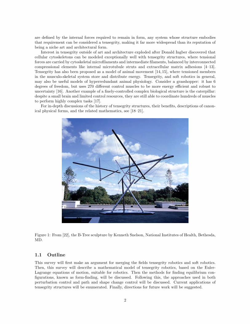
All of these definitions capture the major feature of tensegrity structures: struts do not touch eachother. Since cables can withstand tension, an art form quickly arose in which struts appear to belevitated above ground (Figure 1) embedded in a network of cables. This picture is the predominantimage in tensegrity literature, and the foundation for most of the structural and control research, butthe definition allows a much broader interpretation. The most common deviation from the discon-nected strut model is the appearance of Class 2 tensegrity structures, in which multiple struts arealllowed to touch, but tensioned elements are still a requirement for stability. But tensegrity can befurther generalized. Replace rod-like and cable-like elements with soft surfaces that resist tension andcompression, and the result is a soft robot that does not resemble the canonical art form. Replace thoseelements with microfilaments and microtubules, and the result is a cell [4]. Because tensegrity forms

1

are defined by the internal forces required to remain in form, any system whose structure embodiesthat requirement can be considered a tensegrity, making it far more widespread than its reputation ofbeing a niche art and architectural form.

Interest in tensegrity outside of art and architecture exploded after Donald Ingber discovered thatcellular cytoskeletons can be modeled exceptionally well with tensegrity structures, where tensionalforces are carried by cytoskeletal microfilaments and intermediate filaments, balanced by interconnectedcompressional elements like internal microtubule struts and extracellular matrix adhesions [4–13].Tensegrity has also been proposed as a model of animal movement [14, 15], where tensioned membersin the musculo-skeletal system store and distribute energy. Tensegrity, and soft robotics in general,may also be useful models of hyperredundant animal physiology. Consider a grasshopper: it has 6degrees of freedom, but uses 270 different control muscles to be more energy efficient and robust touncertainty [16]. Another example of a finely-controlled complex biological structure is the caterpillar:despite a small brain and limited control resources, they are still able to coordinate hundreds of musclesto perform highly complex tasks [17].

For in-depth discussions of the history of tensegrity structures, their benefits, descriptions of canon-ical physical forms, and the related mathematics, see [18–21].

Figure 1: From [22], the B-Tree sculpture by Kenneth Snelson, National Institutes of Health, Bethesda,MD.

1.1 Outline

This survey will first make an argument for merging the fields tensegrity robotics and soft robotics.Then, this survey will describe a mathematical model of tensegrity robotics, based on the Euler-Lagrange equations of motion, suitable for robotics. Then the methods for finding equilibrium con-figurations, known as form-finding, will be discussed. Following this, the approaches used in bothperturbation control and path and shape change control will be discussed. Current applications oftensegrity structures will be enumerated. Finally, directions for future work will be suggested.

2

1.2 Tensegrity Structures in Soft Robotics

Soft robotics is a growing field that is becoming more popular as computational and manufacturingabilities have grown to facilitate their study. Soft robots are compliant, have dexterous mobility al-lowing them to working in unstructured and cluttered environments, and can easily deform, all ofwhich allow them to safely interact with people and fragile objects [23]. Whereas traditional robotsrely on rigid components and typically have only as many degrees of freedom as they require for theirworkspaces, soft robots have continuous deformation and therefore have infinite degrees of freedom.While this may appear to make the task of motion planning and manipulation intractable, its appear-ances in nature are ubiquitous. Tongues, elephant trunks, octopus arms, caterpillars, and slugs arejust a few examples.

Possibly due to its reputation as a niche art form, the tensegrity robotics research community barelyoverlaps the soft robotics field as a whole, despite the very similar goals of recent tensegrity roboticistsand soft roboticists. The soft robotics survey [23] does not include a single mention of tensegrity, andyet, modeling and control methods employed in tensegrity robotics research may be directly appliedto the general problems of soft robotics.

Soft robots have few or no rigid members [23], so at first glance it is unclear how tensegrityrobots can be considered soft. However, the lack of distinct rigid members does not mean there isno compression in a soft robot; a system entirely in tension would collapse. Because of this, anycomputational model of a soft robot must be an implicit tensegrity model, even if the distinctionbetween cables and struts is not obvious. For example, an inflated balloon can be considered atensegrity structure, where the surface is fully tensioned, but the compression force from the airprevents collapse. This means that robots composed of pneumatic cells [24] are, in the broad definition,tensegrity robots.

One advantage of tensegrity robots is that they can be modeled as a system of ordinary differen-tial equations, without joint constraints, instead of requiring partial differential equations and theirassociated solution methods (ie. finite element method), which can require long computation times. Amajor challenge in soft robotics is the modeling, control, and path-planning of continuous deformablerobots [23]. However, if these models can be transformed into general tensegrity models, suitablecontrol schemes may arise. Much work has been done in controlling tensegrity robots using varioustechniques (Section 3.3); these methods may be applicable to soft robots in general. Casting a softrobotics problem as a tensegrity problem may not only open up research time for consideration ofadvanced control methods, but may allow such simulations to occur in real time onboard a soft robot,giving the robot the ability to plan its own path through state space.

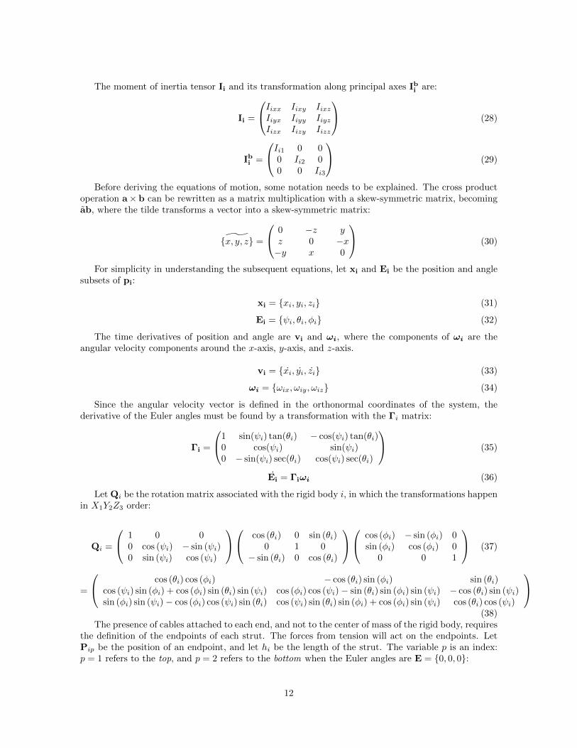
The high degree of coupling in soft robotics leads to hyperredundancy and the capacity for commu-nication between members, allowing for a distributed control system (which is itself another inspirationfrom the world of biology). These things are also true for tensegrity structures. Tensegrity elementsmay simultaneously actuate, sense, and provide feedback for control [25,26]. This notion of mechanicalelements being able to sense, communicate, and provide feedback is known in the literature as mor-phological computation [26, 27], and such structures are known as smart structures [28]. Harnessingthese capabilities allows for the reduction in the number of actuators needed to perform movementand other tasks. For example, the structure shown in Figure 12 has 24 degrees of freedom and can becontrolled by just 2 two-state actuators [27]. Another benefit of this dynamic coupling and actuationis that tensegrity robots could sustain multiple internal failures and still operate as intended. Thisgives tensegrity soft robots the desirable property of robustness.

1.3 Features of Tensegrity Robots

The favorable properties of tensegrity structures have fostered an increasing interest in using tensegritystructures in a wide range of applications. In particular, recent discoveries in biology have helpedto spur a shift from the exploration of static tensegrity structures to its possible uses in roboticapplications. These favorable properties, some of which are summarized in [19,29], are as follows:

3

Figure 2: Comparison of hard and soft robotics, with a soft tensegrity robot analogue. Left, from[23]:Capabilities of hard and soft robots: (a) dexterity, (b) position sensing, (c) manipulation and (d)loading. Right, from [16]: Movement sequence of a planar tensegrity robot with fixed-length struts(cross-diagonal lines) and adjustible control tendons (all others).

Reconfigurability : Tensegrity structures are malleable and can change their structure to accomplishunusual tasks not allowed in the conventional robot [16]. Figure 2 shows a possible reconfigurationsequence for a planar tensegrity robot. This lends itself to unconventional locomotion principles [30].Due to the property that a localized force on a tensegrity structure yields a global change of shape,independent from the position of the actuator, locomotion over rough terrain is possible with few actu-ators [30]. Tensegrity structures may also be collapsed, which has opened it up for orbital deploymentapplications, such as antennae and masts [31,32], where compact storage is the driving motivation forspace structure design. For robots, this property makes tensegrity structures ideal for maneuveringaround tight places, or deforming under large loads instead of failing.

Efficiency : The control of tensegrity structures requires less energy because some of the energyis stored in the structure itself [15]. Actuation releases some of the potential energy, which can beharnessed, and most of which is recaptured instead of being lost to friction. After movement, thepre-stress energy will still remain in the structure. Actuation of one part of a tensegrity structureaffects every other member, allowing for fewer actuators [27].

Failure tolerance: As redundant, dynamically coupled structures, tensegrity robots can perfomtasks reliably even when one or more elements fail [27, 33–36]. This is in contrast to conventionalrobots, in which the failure of a single element may lead to global failure.

Simplicity of design: Highly maneuverable, scalable, and redundant tensegrity robots can be com-posed of a minimum of two kinds of components: passive/actuated struts and passive/actuated cables.This eliminates the need to design each individual component separately. Many prototypical modelschoose one element type to be active while leaving the other passive. Other designs may consider acombination of passive and actuated elements of the same type in a structure.

Ease of modeling : Elements experience only axial forces; not bending moments or shear forces,which makes the computational modeling simpler to devise. Classical flexible structures require partialdifferential equations, which are difficult both analytically and numerically. Tensegrity models, whichonly need to consider axial forces, can be solved with ordinary differential equations [37].

4

2 Tensegrity Model

To create a computational model of a tensegrity robot, the mathematical models of the statics anddynamics must first be described. Not every combination of struts and cables yields a stable tensegritystructure, and indeed, finding new forms is nontrivial. This is known as the form-finding problemand has been the subject of extensive research, much of which has been surveyed by [29, 38, 39]. Theform-finding process is an integral part of the control problem; most control problems are posed as atransformation from one equilibrium form to another, usually following a path made of equilibria.

Before describing the form-finding and control problems, this survey will define the mathematicalmodels of tensegrity forms, in the contexts of both force equilibrium and minimum potential energy.Following this, the two most common dynamical models will be described: one in which tensegritystructures are composed of point masses at the nodes connected by springs, and one in which strutsare rigid bodies connected by springs.

The equations of motion are explicitly derived from Lagrangians in many papers. However, inmany cases, an off-the-shelf physics engine is used. In the latter case, the features are provided bythe library of choice are used [27, 34–36], including rigid bodies, springs, gravity, collision forces, andfriction forces. The benefit of using a physics engine is that it permits researchers to quickly assembleprototypes as a basis for complicated AI control systems. One weakness of this approach is that thereal-time focus of a physics engine like Open Dynamics Engine may not be suitable for high fidelitysimulations of Hamiltonian systems.

2.1 Definitions

While the definition proposed by Fuller is a wide umbrella, many researchers choose to model tensegritystructures as collections of one-dimensional spring-like (or rigid) objects. This allows only compressionand tension forces to be considered, and in turn, allows the use of ODEs, as opposed to PDEs, whichare required for structures in general.

Strut : A strut is a compressed element, usually modeled as a rod or a rigid body. Nearly all researchgroups model struts as straight rods that do not experience bending, shear, or torsional forces, onlycompression. The only exception to this is in [30], which uses curved struts, but the internal forces arenot modeled.

Cable: A cable is a tensioned element, usually modeled as a string or as a spring. Cables are almostuniversally modeled as strings that experience only tension forces. [40] expands the cable concept toinclude tension surfaces, which are modeled in ODE as soft bodies: lattices of point masses connectedby springs.

The topology of tensegrity structures can be expressed as a graph. Tensegrity structures can beclassified into a set of edges, which represent the elements of the structure, and nodes, which arethe locations at which elements meet. Let the abstract tensegrity framework [41] be a graph G(V,E)where the vertices V = 1, . . . , Nv is the set of nodes, and the edges E = 1, . . . , Ne are the set ofelements, where E = C ∪S if only cables and struts are considered, and E = C ∪S ∪B if a third typeof element called a bar, which is allowed to experience both compression and tension, is considered.Cables require an upper bound on their length, struts require a lower bound, and bars have a fixedlength. Alternately, an edge e = u, v may be defined as a pair of vertices.

A tensegrity framework is a pair (G,p) with a position function pi : v ∈ V → Rd mapping thevertices to a d-dimensional position. The vector of all positions, p = (p1

T , . . . ,pNvT ), is the embedding

of the topological structure into Euclidean space. The rigidity matrix [42] R is an Ne × dNv matrixthat maps embeddings to edges (Equation 1). For all edges e ∈ E = u, v, each edge row has dcolumns for each of the Nv vertices.The equilibrium matrix is the transpose of the rigidity matrix [43].Tensegrity structures have multiple embeddings if each embedding cannot be transformed to another bya combination of translations, rotations, and reflections. If these multiple embeddings can be reachedthrough continuous deformations that maintain all edge lengths, it is said to be a mechanism. Furtherdefinitions that are relevant to static analysis can be found in [29,39].

5

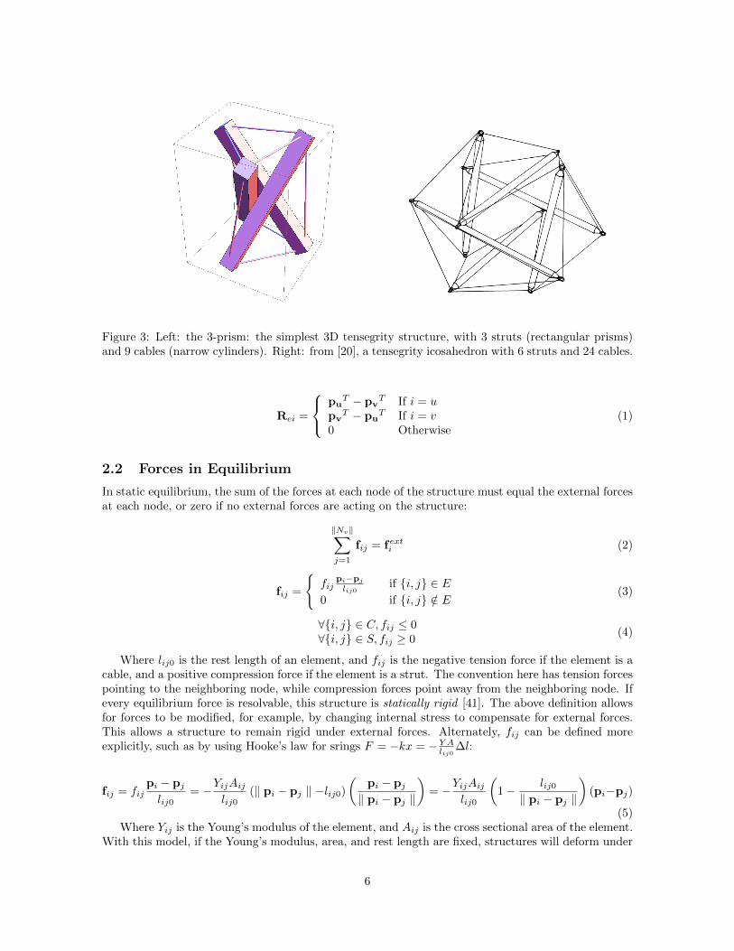
Figure 3: Left: the 3-prism: the simplest 3D tensegrity structure, with 3 struts (rectangular prisms)and 9 cables (narrow cylinders). Right: from [20], a tensegrity icosahedron with 6 struts and 24 cables.

Rei =

puT − pv

T If i = upv

T − puT If i = v

0 Otherwise(1)

2.2 Forces in Equilibrium

In static equilibrium, the sum of the forces at each node of the structure must equal the external forcesat each node, or zero if no external forces are acting on the structure:

‖Nv‖∑j=1

fij = fexti (2)

fij =

fij

pi−pj

lij0if i, j ∈ E

0 if i, j /∈ E(3)

∀i, j ∈ C, fij ≤ 0∀i, j ∈ S, fij ≥ 0

(4)

Where lij0 is the rest length of an element, and fij is the negative tension force if the element is acable, and a positive compression force if the element is a strut. The convention here has tension forcespointing to the neighboring node, while compression forces point away from the neighboring node. Ifevery equilibrium force is resolvable, this structure is statically rigid [41]. The above definition allowsfor forces to be modified, for example, by changing internal stress to compensate for external forces.This allows a structure to remain rigid under external forces. Alternately, fij can be defined moreexplicitly, such as by using Hooke’s law for srings F = −kx = −Y Alij0 ∆l:

fij = fijpi − pjlij0

= −YijAijlij0

(‖ pi − pj ‖ −lij0)

(pi − pj‖ pi − pj ‖

)= −YijAij

lij0

(1− lij0‖ pi − pj ‖

)(pi−pj)

(5)Where Yij is the Young’s modulus of the element, and Aij is the cross sectional area of the element.

With this model, if the Young’s modulus, area, and rest length are fixed, structures will deform under

6

Static equilibrium definitionsV The set of nodes (joints)E The set of edges (struts or cables)Nv The number of nodesNe The number of edgesd The dimension (may be 2 or 3)C ∈ E The set of cablesS ∈ E The set of strutsB ∈ E The set of barsG(V,E) Abstract tensegrity frameworkpi Position of ith nodep Vector of positions(G,p) Tensegrity frameworkR Rigidity matrixRT Equilibrium matrixfij Force vector on node i from node jfij Magnitude of force on node i from node jlij0 Rest length of edge between i, j, where fij = 0fexti External forces on node iYij Young’s modulus of edge between i, jAij Cross-sectional area of edge between i, jqij Force density: force per length of edge between i, jq Stress vector of all force densitiesVij Potential energy of an edge i, jΩ Stress matrixC Stiffness coefficient matrixH Second derivative (Hessian) matrix

Table 1: Static equilibrium definitions.

external loads. The Hooke’s law model of tensegrity structures is especially relevant to robotics. Toenable movement, experiments modify only the rest lengths through actuaion, and no other materialproperties of the structure are changed. Equation 5 is nonlinear, but [44] introduced a way to linearizethe force density qij [44] of each element (force/length) into the system:

qij =fijlij0

(6)

fijpi − pjlij0

= qij(pi − pj) (7)

It is important to point out that equation 7 is only valid if the tendon rest length is 0, which doesnot agree with the Hookean model. The reason for this is that all qij are assumed to be constant,meaning the expression qij(pi−pj) = 0 only when pi = pj . Using the force density linearization, if wedefine the stress vector q ∈ RNe = (. . . , qij , . . . ) to be the vector of all force densities, then equation 2can be rewritten as:

RTq = fext (8)

This results in a linear system that uses the equilibrium matrix [44] and can be solved with linearalgebra methods. For an in-depth analysis of forces in equilibrium, see [29].

7

Point mass dynamic model definitionsmi Mass of node ipi Position of node ifdij Spring damping force magnitude on node i from node jcij Coefficient of damping on edge i, jRigid body dynamic model definitionsi ith rigid bodyip Node, identified by the ith rigid body, and p ∈ 1, 2 is the location (1=top,2=bottom)a Cross product matrix for vector ami Mass-inertia matrixIi Moment of inertia tensorIbi Moment of inertia tensor along principal axespi Rigid body state vector xi, yi, zi, ψi, θi, φixi Position subset of rigid body state vector xi, yi, ziEi Euler angle subset of rigid body state vector ψi, θi, φivi Translational velocity xi, yi, ziωi Angular velocity ωix, ωiy, ωizEi Euler angle derivative with respect to time ψi, θi, φiΓi Matrix that transforms ωi to Ei

Qi Rotation matrix for rigid body iFi Force vector for rigid body iτi Torque vector for rigid body iCT , CR Translational and rotational damping constanthi Length of rigid body iPip Position of node on rigid body i, location pLipjq Length of edge between node ip and node jqLipjq0 Rest length of edge between node ip and node jqFipjq Force acting on rigid body i at node ip from node jqτ ipjq Torque acting on rigid body i at node ip from node jq

Table 2: Dynamics definitions.

2.3 Minimum Potential Energy

Tensegrity systems can also be modeled in terms of the potential energy stored within springs. A rigidtensegrity framework exists when the energy function is at a local minimum [42, 45]. Two conditionsmust be satisfied: the first derivative of the energy function must be 0 at the equilibrium point, andthe second derivative must be positive at the equilibrium point. For a spring obeying Hooke’s law, thepotential energy of a spring is:

Ve =1

2kx2 =

Y A

2le0∆l2 (9)

Vij =

YijAij

2lij0(‖ pi − pj ‖ −lij0)2 if i, j ∈ E

0 if i, j /∈ E(10)

V =∑ij

YijAij2lij0

(‖ pi − pj ‖ −lij0)2 (11)

The first derivative of the energy function must be 0 at the equilibrium point:

dVdt =

∑ij

YijAij(‖pi−pj‖−lij0)

lij0‖pi−pj‖(pi−pj)·(pi−pj)=0 (12)

8

The second derivative must be positive at the equilibrium point:

d2Vdt2 =

∑ijYijAij

lij0

(((pi−pj)·(pi−pj))

2

‖pi−pj‖2

− (‖pi−pj‖−lij0)((pi−pj)·(pi−pj))2

‖pi−pj‖3

+(‖pi−pj‖−lij0)‖pi−pj‖2((pi−pj)·(pi−pj))

‖pi−pj‖

)> 0

(13)

The equilibrium equations listed here are more thoroughly explored in two previously publishedsurveys ( [29,38]).

Equations 9-13 are nonlinear and difficult to work with. Therefore, first appearing in [42], theseare simplified following the same linearization reasoning that resulted in equation 8. First, Hooke’slaw can be replaced with an arbitrary energy function vij of the squared distance between the nodes:

V =∑ij

vij(‖ pi − pj ‖2) (14)

dVdt =

∑ij 2(pi−pj)·(pi−pj) ˙vij(‖pi−pj‖2)=0 (15)

d2Vdt2

=∑

ij 4((pi−pj)·(pi−pj))2vij(‖pi−pj‖2)

+2‖pi−pj‖2(pi−pj)·(pi−pj) ˙vij(‖pi−pj‖2)≥0(16)

The px terms can be left out [29,42], reducing equation 16 to:

d2Vdt2

=∑

ij 4((pi−pj)·(pi−pj))2vij(‖pi−pj‖2)

+2‖pi−pj‖2 ˙vij(‖pi−pj‖2)≥0(17)

The term ˙vij(‖ pi−pj ‖2) can be considered a force density coefficient qij that populates the stressvector q. Thus, equation 15 can be stated:

dV

dt= 2qRp = 0 (18)

To find a similar matrix equation for equation 17, a few new definitions must be made. Let Ω bea stress matrix such that:

Ωij =

−ωij if i 6= j∑k ωik if i = j

(19)

Now let the stiffness coefficient be cij = vij(‖ pi − pj ‖2), and C be the full matrix of cij , thenequation 17 can be stated as a Hessian matrix H of second derivatives:

H = pT [2Ω + 4RTCR]p (20)

When H is positive definite, the energy will be at a minimum, indicating an equilibrium state. Ifequations 18 and 20 can be solved, an equilibrium form will be found. Solutions are not trivial andstraightforward, but several form-finding methods have been found that work reasonably well in manycases.

2.4 Point Mass Lagrangian Equations of Motion

In this model of tensegrity structures, each node is a point mass; struts and cables are modeled assprings. This model is developed thoroughly in [46]. This allows for a simplied model, one withoutrotational velocities or torques, and may only be a rough approximation. One benefit that the pointmass model has over the rigid body model is that singularities arising from gimbal lock can be avoided[39]. The generalized coordinates q can be represented by a vector pi = pix, piy, piz. For a pointmass mi, the kinetic energy is Ti = 1

2miv2i , the potential energy of a point mass due to gravity is

9

Vi = migpiz, and the potential energy of a spring is Vij = 12kij∆l

2. The dissipative forces may bedefined many ways, including as damping on nodes only or damping on the springs, and friction maybe included.

The Lagrangian of a system is the kinetic energy minus the potential energy:

L = T − V (21)

The Euler-Lagrange equations of motion, for a set of generalized coordinates q = q1, q2, ..., qn,are:

ddt

(δLδqi

)− δL

δqi= 0 (22)

For a conservative nodal point mass tensegrity structure under gravity, the full Lagrangian L of asystem is:

L =∑Nv

i12mipi · pi

−∑Nv

i migpiz−∑Ne

ij12kij(‖ pi − pj ‖ −lij0)2

(23)

Applying this system to equation 22 defines the equations of motion for a conservative nodal pointmass tensegrity structure under gravity:∑Nv

i (mipi +migz)

+∑Ne

ij kij(‖ pi − pj ‖ −lij0)pi−pj

‖pi−pj‖ = 0(24)

Note that the spring forces in equation 24 are a restatement of the spring forces in equation 5. Thissystem of equations can be inserted as-is into an integrator such as the Runge-Kutta 4th order solver.A fictional spring damping force may be applied, which can be stated as Fd = −cdxdt . When recast asa function of ‖ pi − pj ‖, the spring damping force becomes:

fdij = −cij(pi − pj) · (pi − pj)

‖ pi − pj ‖(25)

Alternately, a point mass damping model can be applied:

fdi = −cipi (26)

Either way, the damping model serves only one purpose, and that is to allow tensegrity structuresto return to a steady state after a perturbation. Thus, damping is a form of dynamic relaxation.

2.5 Rigid Body Lagrangian Equations of Motion

This model, explicitly defined in [25, 37, 39, 47] and implicit in [26, 27, 34–36], trades the coarse nodalpoint mass model for a model in which each strut is a rigid body, and each cable is modeled as apair of equal but opposite forces acting at the tips of two rigid bodies. Rigid bodies are suitable forsystems in which the struts deform so insignificantly as to be ignored, but they introduce additionalissues. They are also more accurate because the centers of mass are located at the centers of struts,instead of at nodes. Variants of this model simplify the generalized coordinates wherever possible. ANewtonian model for tensegrity shells was converted to a non-linear system of equations where thefirst and second derivatives of strut lengths are constrained to be 0, making them rigid, but leavingout rotational inertia [48–50]. This model was expanded by [51–54] who added a nonlinear model ofelasticity and the deformability of edges.

The model presented here will include no constraints: that is, every body is free to move and rotatealong any axis. A rigid body has six position coordinates: three translational, and three angular. Eulerangles provide a convenient minimized set of angular coordinates. The generalized coordinates for a

10

rigid body are its position and orientation in Euler angles pi = (xi, yi, zi, ψi, θi, φi). Since a body mayrotate around the load axis φ, but none of the cable and strut forces act on that axis in most tensegritymodels, φi is often dropped. However, a generalized strut (that is, something other than a rod) mayrequire modeling of all states, so they will be kept here.

In the point mass notation, both nodes and point mass bodies could be represented by the sameindex i. Here, each rigid body is represented by an index i, and each rigid body has two nodes, whichwill be distinguished with an additional index p, so that a node is identified by the string ip, where iis the body, and p ∈ 1, 2 is the specific location.

Figure 4: A labeled rigid body tensegrity 3-prism. All 6 nodes have positions labeled as Pip, wherei is the identity of the body, and p identifies which of the two endpoints (top=1, bottom=2) is beingconsidered. The center of body 1, p1, is shown. The tension force vectors are shown in red, and arelabeled Fipjq, where the first two digits identify the body and endpoint on which the force is acting,and the second two digits identify the body and endpoint on the opposite end.

A rigid body has a 2d× 2d mass-inertia matrix mi:

mi =

mi 0 0 0 0 00 mi 0 0 0 00 0 mi 0 0 00 0 0 Iixx Iixy Iixz0 0 0 Iiyx Iiyy Iiyz0 0 0 Iizx Iizy Iizz

(27)

11

The moment of inertia tensor Ii and its transformation along principal axes Ibi are:

Ii =

Iixx Iixy IixzIiyx Iiyy IiyzIizx Iizy Iizz

(28)

Ibi =

Ii1 0 00 Ii2 00 0 Ii3

(29)

Before deriving the equations of motion, some notation needs to be explained. The cross productoperation a× b can be rewritten as a matrix multiplication with a skew-symmetric matrix, becomingab, where the tilde transforms a vector into a skew-symmetric matrix:

˜x, y, z =

0 −z yz 0 −x−y x 0

(30)

For simplicity in understanding the subsequent equations, let xi and Ei be the position and anglesubsets of pi:

xi = xi, yi, zi (31)

Ei = ψi, θi, φi (32)

The time derivatives of position and angle are vi and ωi, where the components of ωi are theangular velocity components around the x-axis, y-axis, and z-axis.

vi = xi, yi, zi (33)

ωi = ωix, ωiy, ωiz (34)

Since the angular velocity vector is defined in the orthonormal coordinates of the system, thederivative of the Euler angles must be found by a transformation with the Γi matrix:

Γi =

1 sin(ψi) tan(θi) − cos(ψi) tan(θi)0 cos(ψi) sin(ψi)0 − sin(ψi) sec(θi) cos(ψi) sec(θi)

(35)

Ei = Γiωi (36)

Let Qi be the rotation matrix associated with the rigid body i, in which the transformations happenin X1Y2Z3 order:

Qi =

1 0 00 cos (ψi) − sin (ψi)0 sin (ψi) cos (ψi)

cos (θi) 0 sin (θi)0 1 0

− sin (θi) 0 cos (θi)

cos (φi) − sin (φi) 0sin (φi) cos (φi) 0

0 0 1

(37)

=

cos (θi) cos (φi) − cos (θi) sin (φi) sin (θi)cos (ψi) sin (φi) + cos (φi) sin (θi) sin (ψi) cos (φi) cos (ψi)− sin (θi) sin (φi) sin (ψi) − cos (θi) sin (ψi)sin (φi) sin (ψi)− cos (φi) cos (ψi) sin (θi) cos (ψi) sin (θi) sin (φi) + cos (φi) sin (ψi) cos (θi) cos (ψi)

(38)

The presence of cables attached to each end, and not to the center of mass of the rigid body, requiresthe definition of the endpoints of each strut. The forces from tension will act on the endpoints. LetPip be the position of an endpoint, and let hi be the length of the strut. The variable p is an index:p = 1 refers to the top, and p = 2 refers to the bottom when the Euler angles are E = 0, 0, 0:

12

Pip = Qi

00

hi

2 if p = 1

−hi

2 if p = 2

+

xiyizi

(39)

Pi1 =

12hi sin (θi) + xi

yi − 12hi cos (θi) sin (ψi)

12hi cos (θi) cos (ψi) + zi

(40)

Pi2 =

xi − 12hi sin (θi)

12hi cos (θi) sin (ψi) + yizi − 1

2hi cos (θi) cos (ψi)

(41)

Let i, p be the body and endpoint indices for the body on which a force is acting, and j, q be theindices for another body whose forces are acting on body i. The length of a cable is represented by:

Lipjq = ||Pip −Pjq|| (42)

The rest length is represented by:

Lipjq0 (43)

With all of these definitions, the Lagrangian can be stated. The kinetic energy term is:

T =∑i

1

2viTmivi +

∑i

1

2ωi

T Iiωi (44)

The potential energy term is the gravitational energy plus the stored energy of the springs:

V =∑ij

YijAij

2Lipjq0(Lipjq − Lipjq0)2 if Lipjq > Lipjq0, and cable exists between Pip,Pjq

0 otherwise(45)

The full derivation is beyond the scope of this document, but it results in the Newton Eulerequations. Euler’s equations of motion for a rigid body under torque are:

Iiωi + ωi × (Iiωi) = τi (46)

Solving for ωi:

ωi = Ii−1(τi − ωi × (Iiωi)) = Ii

−1(τi − ωiIiωi) (47)

The transformations of the inertia tensor (and its inverse) from principal axes to system axes are:

Ii = QiIbi QT

i (48)

Ii−1 = Qi(I

bi )−1QT

i (49)

From equations 31-49, the system of ODEs for body i with respect to the derivatives of the statevector pi can be found as a function of the principal inertia tensor parameter Ibi , the mass parametermi, the force vector Fi, the torque vector τi, (and optional translation damping term CT and rotationdamping term CR):

xi = vi (50)

vi =1

miFi − CTv (51)

13

Ei = Γiωi (52)

ωi = Qi(Ibi )−1QT

i (τi − ωiQiIbi QT

i ωi)− CRω (53)

Equations 50-53 are general solutions for any rigid body. Unfortunately, this derivation has asingularity at θi = π

2 , causing Γi to enter gimbal lock. There are a few ways of dealing with this: oneis to use quaternions instead of Euler angles, but this adds a fourth variable to the angle specification,and unit constraint to be satisfied for the ODE solver; another way is to integrate the rotation matrixQi directly, but this adds six additional variables and another unit constraint. For this model, θi = π

2corresponds to a strut being parallel to the XY plane, which, in practice, seldom occurs due to the lowprobability that for any time step in the integration routine, θi will be close enough to π

2 to triggerthe singularity.

The force on body i from the cable spanning Pip,Pjq is:

Fipjq =

YijAij

Lipjq0

(1− Lipjq0

Lipjq

)(Pjq −Pip) if Lipjq > Lipjq0, and cable exists between Pip,Pjq

0 otherwise(54)

The torque on body i from the cable spanning Pip,Pjq is:

τ ipjq =

(Pip − xi)

T × Fipjq if Lipjq > Lipjq0, and cable exists between Pip,Pjq

0 otherwise(55)

The force terms Fipjq and torque terms τ ipjq, alone, represent an uncontrolled tensegrity structurewith no external forces. With positive CT , CR, any initial unstable configuration will eventually settleinto a local minimal energy state as t → ∞. This is a quick and useful way to perform the taskof form-finding without implementing a specific algorithm, and closely resembles dynamic relaxation.While it does not provide an exact answer since convergence only comes at t = ∞, the calculatedequilibrium structures can be arbitrarily close. It is useful for verifying tensile integrity: every cableshould be longer than its rest length as t → ∞; a valid tensegrity does not exist if at least one cableis slack.

2.6 Constraints

There are two ways of handling constraints: either including the constraints directly in the Lagrangianof the system with Lagrange multipliers [46], or creating penalty force pairs [55] that pushes objects inthe desired direction without changing the total energy of the system. Such constraints include groundcontact friction forces [26, 27], collision rebound forces [26, 27], and surface contact forces [55]. Nodescan be fixed in place by forcing pi = pi = 0. This is a part of the model described in [16, 46, 56], andLagrange multipliers are used to embed the constraints into the equations of motion. Instead of spring

models, some researchers [48] employ length change constraints:d‖pi−pj‖

dt =d2‖pi−pj‖

dt2 = 0Rigid body physics libraries like Open Dynamics Engine allow for built-in collision detection be-

tween rigid bodies, which, like the forces derived in [55], applies elastic penalty forces to separateclipping objects. This approach is favored by [26, 27, 34–36], who simply incorporate ODE’s built incollision system into their models.

3 Control

There are multiple ways of controlling a tensegrity robot, such as applying forces to nodes externally[57,58], but the most frequently used control inputs are modifications to the rest lengths. This makesthe edge rest lengths a function of time:

Lij0 → Lij0(t)Lipqj0 → Lipqj0(t)

(56)

14

Standard rigid robot designs have a number of actuators equal to the dimension of its workspace.For robots that are required to place an end effector at some location regardless of orientation, 3 actu-ators are needed. If orientation is considered, this number becomes 6. Additional degrees of freedomgive robots redundancy, but also give inverse kinematics solvers multiple solutions. Paradoxically,tensegrity robots can be considered both under-actuated [34] and hyper-actuated [16], depending onthe context. Underactuated tensegrity robots usually place actuators on a small number of edges notproportional to the number of edges in the structure. The property that tensegrity structures deformglobally under a single force makes finding the workspace for a single actuator complicated, but mayreveal potential control strategies would normally require multiple actuators on rigid robots. On theother hand, if the number of actuated edges is proportional to the number of edges, the system be-comes hyperredundant. This means that methods that search for forms that place some reference pointat a specific location may find multiple solutions, and multiple paths [16]. Finding such forms, thepaths between them, and methods to reduce unwanted vibrations and errors, constitute the problemof control.

This section will first review the known methods for form-finding, which is important for findingspecific locations for reference points and along paths. Then methods for controlling perturbations inthe structure in the neighborhood of equilibrium forms will be discussed. Finally, this survey will doc-ument methods for changing the shape of a structure, and finding valid paths between configurations.

3.1 Form Finding

Form finding finds solutions to the force equilibrium and minimal energy problems. The task ofidentifying the form taken by a tensegrity structure is known as form-finding. As described in [59],and classified by [29,38], the approaches to this task fall under two major categories:

Static: these attempt to find solutions without iterating edge lengths. These also work well forsimple and symmetric cases, but are intractable in the general case.

Kinematic: these methods consider modifying the lengths of either struts or cables until an equi-librium is found. They work well for simple and symmetric structures, but become intractable for thegeneral case.

3.1.1 Static Form Finding

Analytical solutions: This is analogous to the kinematical method, and characterizes node relationshipsas explicit equations that must be solved [60].

Force-density method : Defined in equations 6-8, this is further elaborated in [38], which concludesthat it is an excellent method for finding new tensegrity structures, especially when lengths are notknown at the start, but not ideal for structures in which some element lengths must be fixed a priori.This method has been modified to include shape-based constraints [61]. The force-density method isthe basis for the iterative algorithm presented in [62], which begins with the topology and iterativelycalculates the force densities and geometry by using rank constraints on the stress matrix and rigiditymatrix. Form finding is further explored in [63,64] with a numerical approach.

Energy method : Also assuming a spring model, this method tries to find local potential energyminima; [45]. This method is closely related to the force-density method. “Super stable” structuresare defined using the energy method [65].

Reduced coordinates: This method, first introduced by [66], first identifies a set of generalized coor-dinates and equations for the struts, and then uses symbolic manipulation software like Mathematicato convert these equations into cable lengths. Structural symmetry is used to reduce the number ofunknowns. This is tractable only when the structure is simple and symmetric.

Axial forces: This method first finds a set of axial forces that fit the topology of the structure, andthen uses that information to find the node coordinates through successive approximation [67].

15

3.1.2 Kinematic Form Finding

Analytical solutions: This is for structures simple enough that the specific translational and angularrelations can be concisely described in equations and first derivatives. If struts are varied, equilibriumis found at the conditions that maximize strut length. Likewise, if cables are varied, equilibrium occursat minimal cable length. It is assumed that struts and cables, while variable overall, are all the samelength within each category. This method is suitable to symmetrical structures [60].

Marching form-finding : This was introduced by [68] as an algorithm that begins with a stableplacement of a given topology, and modifies it by solving a system of differential equations to changethe lengths of members.

Nonlinear programming : This generalizes the analytical solution method by turning it into a con-straint satisfaction problem [69]. In this case, maximizing the lengths of the struts is the objectivefunction, and the constraints keep the lengths of cables constant, and ensure that all struts are thesame. A function like fmincon in Matlab can be used to solve the problem. An advantage is thatthis allows software packages to be used, but as the structure grows, the constraint problem growssignificantly.

Dynamic relaxation: First introduced into tensegrity analysis by [70]. Dynamic relaxation is avariant of straightforward integration of the systems of motion, in which, starting from a “guess”,forces at the nodes are calculated, and the nodes are accelerated in the direction of forces. Thisprocess iterates until forces at each node are in equilibrium. This is modified by [71] to includecontinuous cables that slide over pulleys. [70] concludes this method does not have good convergenceproperties for structures with large numbers of nodes. In [72], dynamic relaxation is combined withartificial neural networks to improve accuracy.

Genetic algorithms: Genetic algorithms may be used to evolve topologies by encoding the connec-tivity graph as a string that is subject to crossover and mutation. This approach has been used to findirregular and asymmetric structures [73–75], and shows a lot of promise for finding new categories oftensegrity structures, instead of building on forms found through intuition. Graph grammar descrip-tions of tensegrity connectivity, combined with genetic algorithms, were proposed by [75] and modifiedby [74] to generate very large irregular structures, and both claim that their methods produce muchlarger novel tensegrities than other literature. Genetic algorithms are further explored by [76], whosemodel is a slight variant, but with similar results.

Sequential quadratic programming : for additional material constraints such as buckling and yieldstress, a quadratic penalty method may be applied to the search algorithm [77]. However, this maynot always converge to an optimal solution.

Finite element method : closely related to dynamic relaxation, a pair of iterative algorithms con-verges a structure based on minimizing both displacements and energy [78].

3.2 Perturbation Control

Perturbation control, that is, the reduction of unwanted vibrations, has been a key area of researchfor static tensegrity structures. However, in the context of robotics, these studies are also useful,especially in systems in which undamped spring-like elements may continue to vibrate even aftera desired control is performed.From a structural standpoint, controlling unwanted vibrations in thestructure is important for ensuring long-term stability. Nearly all of the literature about perturbationcontrol is active; only [48] examines passive control. However, active control requires little controlenergy [19], therefore there has been no pressing need to examine passive control.

Both the point-mass formulation and the rigid body formulation are high-dimensional nonlinearsystems, and are therefore hard control problems. However, near the equilibrium points, these systemscan be linearized as a function of the Jacobian matrix. This allows the system to be controlled usingstandard linear control schemes, such as PID control, optimal control with linear quadratic Guassiancontrol and Model Predictive Control, robust control using H2 and H∞ controllers, and intelligentcontrols. Feedback linearization can be used instead of full linearization. Linearization works well for

16

actively controlling unwanted vibrations, and can provide an approximation for the deformation ofa tensegrity structure under a force perturbation [79]. Of all of the following methods, only [58, 80]actually tested these models in real structures [39].

Classical : The first studies on the perturbation of tensegrity structures was performed by [81, 82]whose model determined the transfer function between an input force and the oscillations arounda linearized model of the tensegrity structure. In [80], two methods are used. One is called localintegral force feedback, which is used in each actuated member to dampen its vibrations. This methodonly controls edges individually using only that edge’s tension as an input. The other method is calledacceleration feedback control, builds upon a global information model found in [83]; this system performsa more effective dampening on the structure as a whole, but is harder to implement. [19, 37, 84, 85]also defined a simple prototype for an active control system based around linearization around theequilibrium. A two-part control law was devised by [57, 58] for tensegrity planar structures. A PIcontroller is used for filtering out high-frequency displacements. The other part is a robust controlmethod, H∞, accounts for errors in the dynamical system.

Feedback Linearization: Feedback linearization is used by [86,87] to minimize tracking error while atensegrity manipulator robot is undergoing a transformation along a path. It is successful at preventingforces within the cables from reaching an upper limit during a shape reconfiguration.

Optimal : Optimal control schemes seek to minimize changes in the equilibrium lengths of edges [88].In [89], structures undergoing large displacements over time can be controlled via instantaneous optimalcontrol using a linearized version of the model at each step in the transformation. However, the error ofthe linear system is increased due to the extra force being applied by the actuated members. The pointmass model is used in [90] to describe a structure on which a linear quadratic controller is applied tocontrol the linearized dynamics around an equilibrium point. The linear quadratic controller was foundto have great performance. The authors also show that even large deformations can be reasonablyapproximated by a linear model.

Robust : Robust control accounts for errors in both the system and in the measurement of thesystem. A robust control technique, H∞, makes up the second part of the control law in [57, 58].Perturbations are reduced during shape reconfiguration in [91] by using an H2 controller to removeunwanted vibrations. The H2 controller is sufficient in keeping the actual path close to the referencepath.

Machine Learning and Search Methods: A different approach examines the control of structuresin the dynamical state space. A machine learning framework is combined with simulated annealing[92,93] and the Probabilistic Global Search Lausanne (PGSL) [94] method to improve the performanceof tensegrity structures over time. With other tensegrity search methods, the possible lengths arediscretized. The discretized search function is combined with dynamic relaxation to find equilibriumpoints. Since each edge has a finite number of possibilities, the entire space of searchable structuresis exponential with the number of elements, necessitating the inclusion of simulated annealing andPGSL. In [93], this approach is tested with a structure under various loads. A physical tensegritystructure under loads is compared to the numerical method, with the prediction closely matching thetest structure. This approach can be used in real-time in [94], which also includes a machine learningmethod that stores good control commands to further speed up the search. Further tweaks have beenmade to reduce the search space, as in [95, 96], who include artificial neural networks to compensatefor additional effects, and utilize additional criteria such as maximum stiffness and minimum stress.

3.3 Path and Shape Control

Path and shape control is the principal concern of the study of soft robotics control systems, andtherefore is examined in great detail in this survey. Path and shape control concerns the transformationof a tensegrity structure from one feasible configuration to another by finding a path that maintainsthe feasibility of the structure throughout the process. The path requirements range from finding anyfeasible path, to finding a path that minimizes some cost function. This is important for tensegrityrobots, as shape control is expected to be a consistent requirement, as opposed to static tensegrity

17

structures and single deployment structures like space antennae [37]. This is complicated by the factthat tensegrity robots may have obstacles in their workspaces, and the transformation from physicalspace to parameter space is a hard problem. The set of feasible tensegrity structures in equilibrium is alower dimension than the space in which it is embedded; therefore, standard path-planning techniques,such as [97,98] are not practical [39].

There are two very different approaches for judging the quality of a proposed control scheme. Inone camp, the path as a whole is considered as a continuous function on which various control methods,such as open-loop control, optimal control, and Lyapunov control, are applied. The major difficulty inthis is that closed-form solutions are not possible to derive except in highly simplified models, and ingeneral, control of nonlinear systems is difficult, leading to these studies using the simplest symmetricaltensegrity structures. Generally, 2D structures are used in the continuous control literature: the smallerdimension allows for easier searching through state space for candidate solutions to the various problemsproposed in the literature. With symmetry, this can be reduced to a low-dimensional problem.

The other camp discretizes the generation of paths. At various points along the path, including thestart and end, form-finding methods are used to converge to equilibrium points, and the remainder ofthe path is generated by simply actuating to get from one length to the next. Discrete problems aresuitable for graph search methods and artificial intelligence techniques. They also are more commonlyused for irregular and large tensegrity structures. Three-dimensional structures, where considered, areusually simple and used for proofs of concept [55], due to the computational complexity of simulatinglarge tensegrity structures with large parameter dimensions. The intelligent control methods usedin [27, 99] buck this trend by showing that large and irregular structures can be controlled if thecontrol specifications are simple enough (such as translation along a path).

3.3.1 Continuous Path Control

When the shape change control problem is considered as a continuous function, standard controltheory techniques, ranging from open loop to PID to optimal control, are considered. The structuresconsidered in these problems are highly symmetric and simple, reducing the parameter dimensionconsiderably. While the result presented here are sufficient, it remains to be seen if these techniquescan be used in more complicated structures.

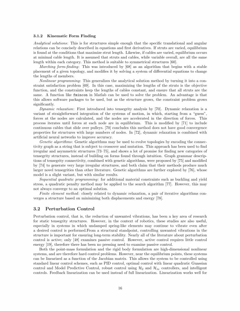
Reconfiguration to a specific state, no path optimization:Slowly varying transformations are con-sidered as an open loop quasi-static path control [100–103]. Their solution is to use slowly varyingfunctions that move a structure from one equilibrium configuration to another along a path. By movingslowly between equilibrium configurations, the problem of unwanted nonlinear dynamics is ignored.By using a highly symmetric tensegrity system, the path has a closed form solution. Figure 5 showsthe deployment process.

A PID controller is proposed in [104]. Here, Cartesian coordinates of the workspace are mapped tothe parameter space of the tensegrity robot, and a PID controller is used to move the robot along thepath. The error of the PID controller fluctuates, due in part to the 2-actuator system controlling a3-DOF system, and damping is insufficient, leading to the PID controller to being a suboptimal choice.

Control based around a differential algebraic equation model of tensegrity structures with con-straints is considered in [105, 106]. Differential algebraic equations are used to avoid the singularitiesthat may occur in the rigid body ODE system. In [105,106], a simple constrained tensegrity structure,essentially a guyed mast with a single strut and three cables, all attached to the ground, is controlledwith two variants of nonlinear Lyapunov control, where the goal is to move the tip of the strut from oneposition to another, and the error is the distance between the current and goal positions. In the firstvariant, the system dynamics themselves are controlled, and in the second, the system is projected toan orthogonal space. Both approaches show convergence to the goal with exponential decay. The con-tributions of these papers are significant in that a nonlinear continuous control scheme is demonstratedfor a three-dimensional tensegrity robot, whereas in other work nonlinear controllers are implementedas either discrete time steps or discretized choices [25, 33, 46, 91, 102, 107], or continuous controllersare used on two-dimensional tensegrity robots [86, 87]. A very detailed description of the differential

18

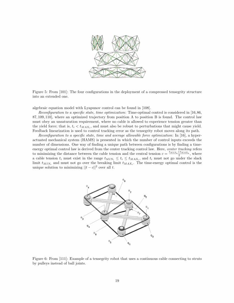
Figure 5: From [101]: The four configurations in the deployment of a compressed tensegrity structureinto an extended one.

algebraic equation model with Lyapunov control can be found in [108].Reconfiguration to a specific state, time optimization: Time-optimal control is considered in [16,86,

87, 109, 110], where an optimized trajectory from position A to position B is found. The control lawmust obey an unsaturation requirement, where no cable is allowed to experience tension greater thanthe yield force; that is, ti < tMAXi , and must also be robust to perturbations that might cause yield.Feedback linearization is used to control tracking error as the tensegrity robot moves along its path.

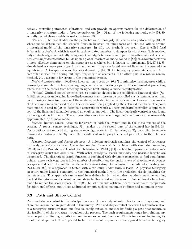
Reconfiguration to a specific state, time and average allowable force optimization: In [16], a hyper-actuated mechanical system (HAMS) is presented in which the number of control inputs exceeds thenumber of dimensions. One way of finding a unique path between configurations is by finding a time-energy optimal control law is derived from the center tracking control law. Here, center tracking refersto minimizing the distance between the cable tension and the central tension c =

tMINi+tMAXi

2 , wherea cable tension ti must exist in the range tMINi

≤ ti ≤ tMAXi, and ti must not go under the slack

limit tMINiand must not go over the breaking limit tMAXi

. The time-energy optimal control is theunique solution to minimizing ||t− c||2 over all t.

Figure 6: From [111]: Example of a tensegrity robot that uses a continuous cable connecting to strutsby pulleys instead of ball joints.

19

Reconfiguration to a specific state, smallest maximum torque optimization: In [111], this controllaw is modified to be a minimal-effort (smallest maximum torque) backlash-free (no slack cables)control law. Here, motors drive cables, and motor torque is proportional to cable tension. The majordifference from [16] is that no upper tension limit is used, but a lower tension limit is enforced. Anoptimal control law is derived that finds the trajectory that minimizes the maximum torque whileensuring that all cables remain taut. Using a control law that minimizes the maximum cable tension(expressed as motor torque) for path following, [111] briefly describes a method for generating non-obstructing paths for snakelike robots like the one shown in Figure 7. To do this, candidates weregenerated and ranked for fitness, where the fitness measure is the smallest angle: large small angles aresaid to be more controllable. Constraints applied to candidates included attaching nodes to splines.However, [16] does not provide additional details of this obstacle course maneuvering model due tospace limitations. Using the system of equations for time-energy optimal control with center trackingdescribed in [16], an iterative guessing algorithm is presented in which one of the parameters of thesystem is guessed, and if the system converges to the final end conditions (the robot has moved toits expected goal), the optimal trajectory is found, and if not, another guess is made and the processrepeats.

Reconfiguration to a specific state, minimize maximum actuation length: Basing the design oftensegrity structures around the ability to control the shape is the main focus of [112]. Of particularinterest is the selection of which edges should be given actuators, as giving all edges actuators isseen as costly. This paper presents mixed integer linear programming, with the objective function ofminimizing the change in length of actuated struts, as an often suitable way to find a good path thatminimizes actuation distance. Its main strength is the ability to be used on-line, with computationtimes roughly equivalent to the amount of time needed to follow the path. However, for rigoroustreatment, mixed integer linear programming is inappropriate.

Figure 7: From [111]: Snakelike motion of a 2D planar tensegrity robot through a simulated obstaclecourse.

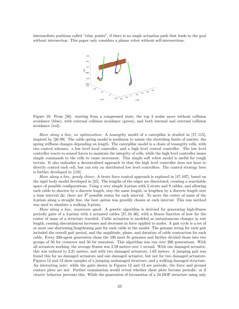
Reconfiguration to a specific state, avoid collision: In [56], a Lyupanov-based control system isused. Here, Model Predictive Control is used to estimate the future behavior of a moving tensegritystructure and choose a control input such that collisions are avoided up to a prediction time horizon.This approached is simulated for a 3-prism, with paths for the top 3 nodes shown in Figure 10.However, the main drawback is that there is no systematic method to find suitable Lyapunov functionsfor arbitrary tensegrity structures, and the time required to search for a suitable control input thatreliably avoids collisions makes it impossible to use in real time.

20

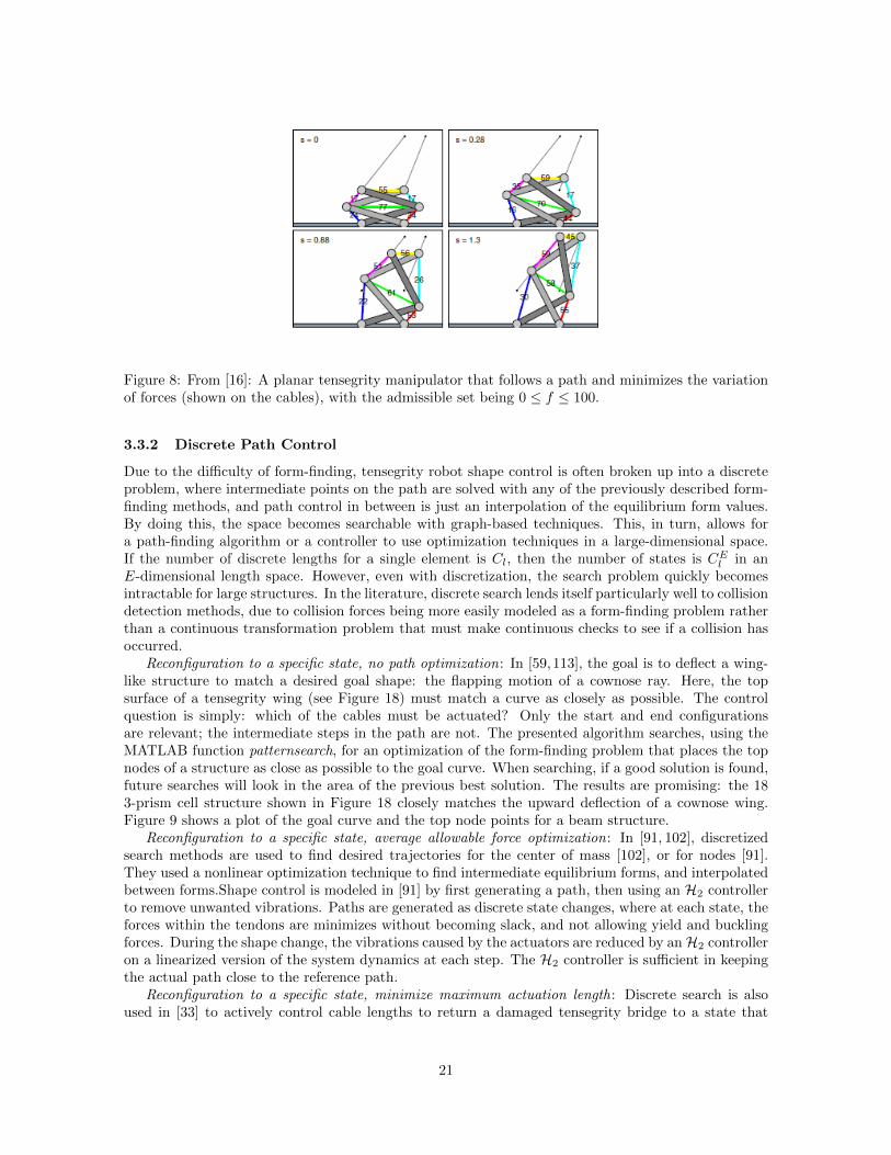
Figure 8: From [16]: A planar tensegrity manipulator that follows a path and minimizes the variationof forces (shown on the cables), with the admissible set being 0 ≤ f ≤ 100.

3.3.2 Discrete Path Control

Due to the difficulty of form-finding, tensegrity robot shape control is often broken up into a discreteproblem, where intermediate points on the path are solved with any of the previously described form-finding methods, and path control in between is just an interpolation of the equilibrium form values.By doing this, the space becomes searchable with graph-based techniques. This, in turn, allows fora path-finding algorithm or a controller to use optimization techniques in a large-dimensional space.If the number of discrete lengths for a single element is Cl, then the number of states is CEl in anE-dimensional length space. However, even with discretization, the search problem quickly becomesintractable for large structures. In the literature, discrete search lends itself particularly well to collisiondetection methods, due to collision forces being more easily modeled as a form-finding problem ratherthan a continuous transformation problem that must make continuous checks to see if a collision hasoccurred.

Reconfiguration to a specific state, no path optimization: In [59,113], the goal is to deflect a wing-like structure to match a desired goal shape: the flapping motion of a cownose ray. Here, the topsurface of a tensegrity wing (see Figure 18) must match a curve as closely as possible. The controlquestion is simply: which of the cables must be actuated? Only the start and end configurationsare relevant; the intermediate steps in the path are not. The presented algorithm searches, using theMATLAB function patternsearch, for an optimization of the form-finding problem that places the topnodes of a structure as close as possible to the goal curve. When searching, if a good solution is found,future searches will look in the area of the previous best solution. The results are promising: the 183-prism cell structure shown in Figure 18 closely matches the upward deflection of a cownose wing.Figure 9 shows a plot of the goal curve and the top node points for a beam structure.

Reconfiguration to a specific state, average allowable force optimization: In [91, 102], discretizedsearch methods are used to find desired trajectories for the center of mass [102], or for nodes [91].They used a nonlinear optimization technique to find intermediate equilibrium forms, and interpolatedbetween forms.Shape control is modeled in [91] by first generating a path, then using an H2 controllerto remove unwanted vibrations. Paths are generated as discrete state changes, where at each state, theforces within the tendons are minimizes without becoming slack, and not allowing yield and bucklingforces. During the shape change, the vibrations caused by the actuators are reduced by anH2 controlleron a linearized version of the system dynamics at each step. The H2 controller is sufficient in keepingthe actual path close to the reference path.

Reconfiguration to a specific state, minimize maximum actuation length: Discrete search is alsoused in [33] to actively control cable lengths to return a damaged tensegrity bridge to a state that

21

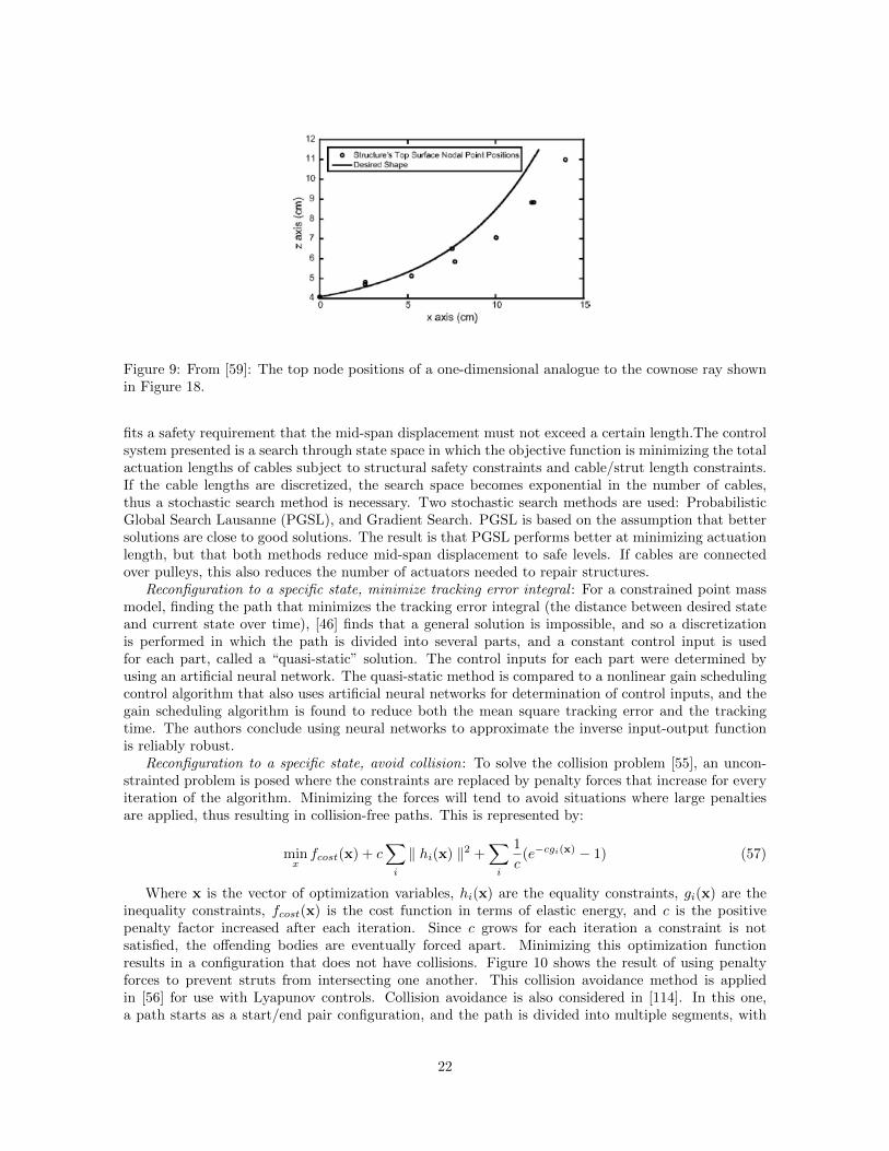
Figure 9: From [59]: The top node positions of a one-dimensional analogue to the cownose ray shownin Figure 18.

fits a safety requirement that the mid-span displacement must not exceed a certain length.The controlsystem presented is a search through state space in which the objective function is minimizing the totalactuation lengths of cables subject to structural safety constraints and cable/strut length constraints.If the cable lengths are discretized, the search space becomes exponential in the number of cables,thus a stochastic search method is necessary. Two stochastic search methods are used: ProbabilisticGlobal Search Lausanne (PGSL), and Gradient Search. PGSL is based on the assumption that bettersolutions are close to good solutions. The result is that PGSL performs better at minimizing actuationlength, but that both methods reduce mid-span displacement to safe levels. If cables are connectedover pulleys, this also reduces the number of actuators needed to repair structures.

Reconfiguration to a specific state, minimize tracking error integral : For a constrained point massmodel, finding the path that minimizes the tracking error integral (the distance between desired stateand current state over time), [46] finds that a general solution is impossible, and so a discretizationis performed in which the path is divided into several parts, and a constant control input is usedfor each part, called a “quasi-static” solution. The control inputs for each part were determined byusing an artificial neural network. The quasi-static method is compared to a nonlinear gain schedulingcontrol algorithm that also uses artificial neural networks for determination of control inputs, and thegain scheduling algorithm is found to reduce both the mean square tracking error and the trackingtime. The authors conclude using neural networks to approximate the inverse input-output functionis reliably robust.

Reconfiguration to a specific state, avoid collision: To solve the collision problem [55], an uncon-strainted problem is posed where the constraints are replaced by penalty forces that increase for everyiteration of the algorithm. Minimizing the forces will tend to avoid situations where large penaltiesare applied, thus resulting in collision-free paths. This is represented by:

minxfcost(x) + c

∑i

‖ hi(x) ‖2 +∑i

1

c(e−cgi(x) − 1) (57)

Where x is the vector of optimization variables, hi(x) are the equality constraints, gi(x) are theinequality constraints, fcost(x) is the cost function in terms of elastic energy, and c is the positivepenalty factor increased after each iteration. Since c grows for each iteration a constraint is notsatisfied, the offending bodies are eventually forced apart. Minimizing this optimization functionresults in a configuration that does not have collisions. Figure 10 shows the result of using penaltyforces to prevent struts from intersecting one another. This collision avoidance method is appliedin [56] for use with Lyapunov controls. Collision avoidance is also considered in [114]. In this one,a path starts as a start/end pair configuration, and the path is divided into multiple segments, with

22

intermediate positions called “relay points”, if there is no single actuation path that leads to the goalwithout intersection. This paper only considers a planar robot without self-intersections.

Figure 10: From [56]: starting from a compressed state, the top 3 nodes move without collisionavoidance (blue), with external collision avoidance (green), and both internal and external collisionavoidance (red).

Move along a line, no optimization: A tensegrity model of a caterpillar is studied in [17, 115],inspired by [26,99]. The cable spring model is nonlinear to mimic the stretching limits of mucles: thespring stiffness changes depending on length. The caterpillar model is a chain of tensegrity cells, withtwo control schemes: a low level local controller, and a high level central controller. The low levelcontroller reacts to sensed forces to maintain the integrity of cells, while the high level controller issuessimple commands to the cells to cause movement. This simple soft robot model is useful for roughterrain. It also embodies a decentralized approach in that the high level controller does not have todirectly control each cell, but can rely on distributed low level controllers. The control strategy hereis further developed in [116].

Move along a line, greedy chioce: A brute force control approach is explored in [47, 107], based onthe rigid body model developed in [25]. The lengths of the edges are discretized, creating a searchablespace of possible configurations. Using a very simple 3-prism with 3 struts and 9 cables, and allowingeach cable to shorten by a discrete length, stay the same length, or lengthen by a discrete length overa time interval ∆t, there are 39 possible states for each interval. To move the center of mass of the3-prism along a straight line, the best option was greedily chosen at each interval. This was methodwas used to simulate a walking 3-prism.

Move along a line, maximum speed : A genetic algorithm is derivied for generating high-fitnessperiodic gaits of a 4-prism with 4 actuated cables [27, 34–36], with a fitness function of how far thecenter of mass of a structure traveled. Cable actuation is modeled as instantaneous changes in restlength, causing discontinuous increases and decreases in force applied to nodes. A gait cycle is a set ofat most one shortening/lengthening pair for each cable in the model. The genome string for each gaitincluded the overall gait period, and the amplitude, phase, and duration of cable contraction for eachcable. Every 200-agent generation chose the 100 most fit genomes and further divided those into twogroups of 50 for crossover and 50 for mutation. This algorithm was run over 200 generations. Withall actuators working, the average fitness was 2.59 meters over 1 second. With one damaged actuator,this was reduced to 2.21 meters, and with two damaged actuators, 1.62 meters. A jumping gait wasfound this for no damaged actuators and one damaged actuator, but not for two damaged actuators.Figures 12 and 13 show samples of a jumping undamaged structure, and a walking damaged structure.An interesting note: while the gaits shown in Figures 12 and 13 are periodic, the force and groundcontact plots are not. Further examination would reveal whether these plots become periodic, or ifchaotic behavior prevents this. While the generation of locomotion of a 24-DOF structure using only

23

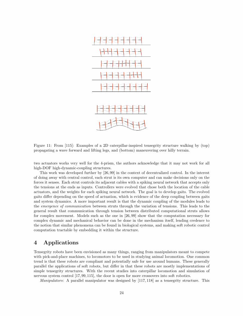
Figure 11: From [115]: Examples of a 2D caterpillar-inspired tensegrity structure walking by (top)propagating a wave forward and lifting legs, and (bottom) maneuvering over hilly terrain.

two actuators works very well for the 4-prism, the authors acknowledge that it may not work for allhigh-DOF high-dynamic-coupling structures.

This work was developed further by [26,99] in the context of decentralized control. In the interestof doing away with central control, each strut is its own computer and can make decisions only on theforces it senses. Each strut controls its adjacent cables with a spiking neural network that accepts onlythe tensions at the ends as inputs. Controllers were evolved that chose both the location of the cableactuators, and the weights for each spiking neural network. The goal is to develop gaits. The evolvedgaits differ depending on the speed of actuation, which is evidence of the deep coupling between gaitsand system dynamics. A more important result is that the dynamic coupling of the modules leads tothe emergence of communication between struts through the variation of tensions. This leads to thegeneral result that communication through tension between distributed computational struts allowsfor complex movement. Models such as the one in [26, 99] show that the computation necessary forcomplex dynamic and mechanical behavior can be done in the mechanism itself, lending credence tothe notion that similar phenomena can be found in biological systems, and making soft robotic controlcomputation tractable by embedding it within the structure.

4 Applications

Tensegrity robots have been envisioned as many things, ranging from manipulators meant to competewith pick-and-place machines, to locomotors to be used in studying animal locomotion. One commontrend is that these robots are compliant and potentially safe for use around humans. These generallyparallel the applications of soft robots, but differ in that these robots are mostly implementations ofsimple tensegrity structures. With the recent studies into caterpillar locomotion and simulation ofnervous system control [17,99,115], the door is open for more crossovers into soft robotics.

Manipulators: A parallel manipulator was designed by [117, 118] as a tensegrity structure. This

24

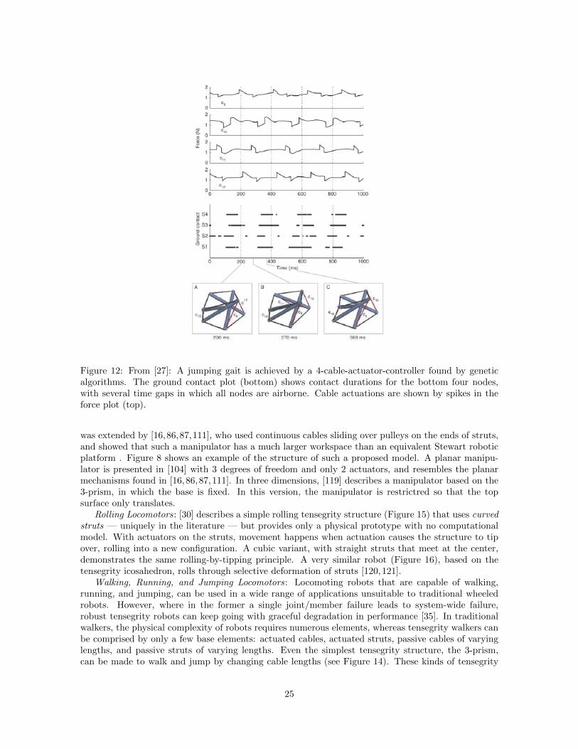
Figure 12: From [27]: A jumping gait is achieved by a 4-cable-actuator-controller found by geneticalgorithms. The ground contact plot (bottom) shows contact durations for the bottom four nodes,with several time gaps in which all nodes are airborne. Cable actuations are shown by spikes in theforce plot (top).

was extended by [16,86,87,111], who used continuous cables sliding over pulleys on the ends of struts,and showed that such a manipulator has a much larger workspace than an equivalent Stewart roboticplatform . Figure 8 shows an example of the structure of such a proposed model. A planar manipu-lator is presented in [104] with 3 degrees of freedom and only 2 actuators, and resembles the planarmechanisms found in [16,86,87,111]. In three dimensions, [119] describes a manipulator based on the3-prism, in which the base is fixed. In this version, the manipulator is restrictred so that the topsurface only translates.

Rolling Locomotors: [30] describes a simple rolling tensegrity structure (Figure 15) that uses curvedstruts — uniquely in the literature — but provides only a physical prototype with no computationalmodel. With actuators on the struts, movement happens when actuation causes the structure to tipover, rolling into a new configuration. A cubic variant, with straight struts that meet at the center,demonstrates the same rolling-by-tipping principle. A very similar robot (Figure 16), based on thetensegrity icosahedron, rolls through selective deformation of struts [120,121].

Walking, Running, and Jumping Locomotors: Locomoting robots that are capable of walking,running, and jumping, can be used in a wide range of applications unsuitable to traditional wheeledrobots. However, where in the former a single joint/member failure leads to system-wide failure,robust tensegrity robots can keep going with graceful degradation in performance [35]. In traditionalwalkers, the physical complexity of robots requires numerous elements, whereas tensegrity walkers canbe comprised by only a few base elements: actuated cables, actuated struts, passive cables of varyinglengths, and passive struts of varying lengths. Even the simplest tensegrity structure, the 3-prism,can be made to walk and jump by changing cable lengths (see Figure 14). These kinds of tensegrity

25

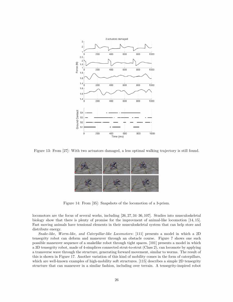
Figure 13: From [27]: With two actuators damaged, a less optimal walking trajectory is still found.

Figure 14: From [35]: Snapshots of the locomotion of a 3-prism.

locomotors are the focus of several works, including [26, 27, 34–36, 107]. Studies into musculoskeletalbiology show that there is plenty of promise for the improvment of animal-like locomotion [14, 15].Fast moving animals have tensional elements in their musculoskeletal system that can help store anddistribute energy.

Snake-like, Worm-like, and Caterpillar-like Locomotors: [111] presents a model in which a 2Dtensegrity robot can deform and maneuver through an obstacle course. Figure 7 shows one suchpossible maneuver sequence of a snakelike robot through tight spaces. [101] presents a model in whicha 3D tensegrity robot, made of 4-simplices connected strut-to-strut (Class 2), can locomote by applyinga transverse wave through the structure, generating forward movement, similar to worms. The result ofthis is shown in Figure 17. Another variation of this kind of mobility comes in the form of caterpillars,which are well-known examples of high-mobility soft structures. [115] describes a simple 2D tensegritystructure that can maneuver in a similar fashion, including over terrain. A tensegrity-inspired robot

26

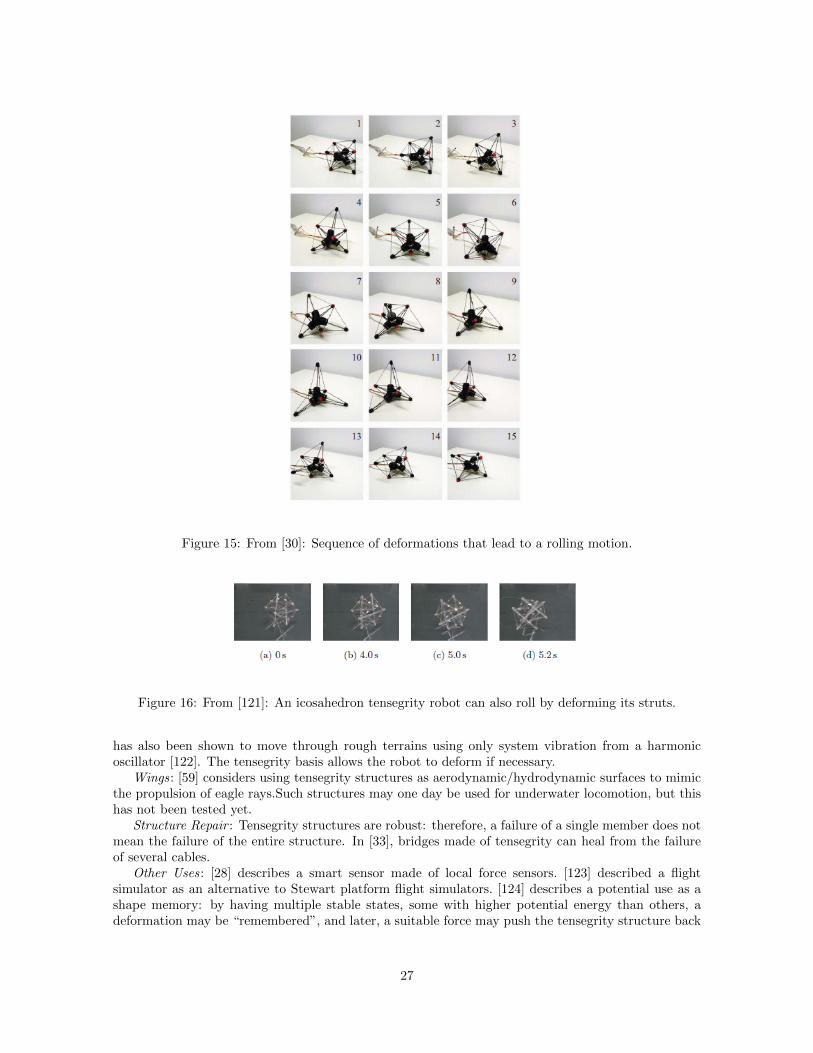
Figure 15: From [30]: Sequence of deformations that lead to a rolling motion.

Figure 16: From [121]: An icosahedron tensegrity robot can also roll by deforming its struts.

has also been shown to move through rough terrains using only system vibration from a harmonicoscillator [122]. The tensegrity basis allows the robot to deform if necessary.

Wings: [59] considers using tensegrity structures as aerodynamic/hydrodynamic surfaces to mimicthe propulsion of eagle rays.Such structures may one day be used for underwater locomotion, but thishas not been tested yet.

Structure Repair : Tensegrity structures are robust: therefore, a failure of a single member does notmean the failure of the entire structure. In [33], bridges made of tensegrity can heal from the failureof several cables.

Other Uses: [28] describes a smart sensor made of local force sensors. [123] described a flightsimulator as an alternative to Stewart platform flight simulators. [124] describes a potential use as ashape memory: by having multiple stable states, some with higher potential energy than others, adeformation may be “remembered”, and later, a suitable force may push the tensegrity structure back

27

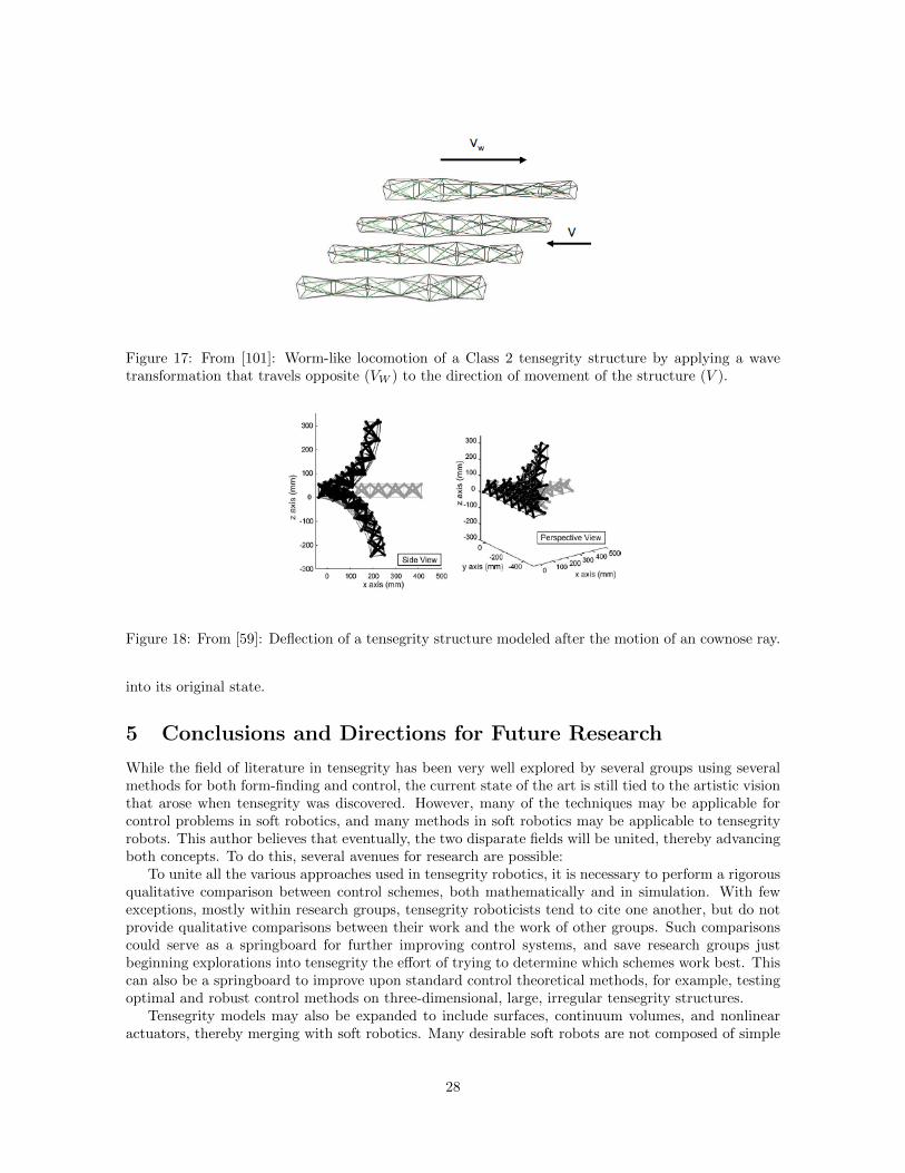
Figure 17: From [101]: Worm-like locomotion of a Class 2 tensegrity structure by applying a wavetransformation that travels opposite (VW ) to the direction of movement of the structure (V ).

Figure 18: From [59]: Deflection of a tensegrity structure modeled after the motion of an cownose ray.

into its original state.

5 Conclusions and Directions for Future Research

While the field of literature in tensegrity has been very well explored by several groups using severalmethods for both form-finding and control, the current state of the art is still tied to the artistic visionthat arose when tensegrity was discovered. However, many of the techniques may be applicable forcontrol problems in soft robotics, and many methods in soft robotics may be applicable to tensegrityrobots. This author believes that eventually, the two disparate fields will be united, thereby advancingboth concepts. To do this, several avenues for research are possible:

To unite all the various approaches used in tensegrity robotics, it is necessary to perform a rigorousqualitative comparison between control schemes, both mathematically and in simulation. With fewexceptions, mostly within research groups, tensegrity roboticists tend to cite one another, but do notprovide qualitative comparisons between their work and the work of other groups. Such comparisonscould serve as a springboard for further improving control systems, and save research groups justbeginning explorations into tensegrity the effort of trying to determine which schemes work best. Thiscan also be a springboard to improve upon standard control theoretical methods, for example, testingoptimal and robust control methods on three-dimensional, large, irregular tensegrity structures.

Tensegrity models may also be expanded to include surfaces, continuum volumes, and nonlinearactuators, thereby merging with soft robotics. Many desirable soft robots are not composed of simple

28

cables and struts; however, surfaces can be modeled as meshes of members separated by springs, andhas been quite successful in the simulation of cloth dynamics. Work toward this goal has been startedin [40], but to date, nothing else has occurred. Expanding the classes of struts and cables could leadto a variety of interesting capabilities, and would better reflect what has been studied in biology. Acurrent challenge in soft robotics is to find accurate models and controllers that describe soft robotics,as current methods are too computationally expensive to be used for real-time control [23]. By castinga soft robotics model as a tensegrity model, this might become tractable.

Research into distributed control systems should also be expanded. This has been done in [17,115],and biologically-inspired distributed control systems were investigated [26, 27]. Combined with anexpanded model of tensegrity structures to include surfaces, many interesting and useful techniquesmay be found to advance the state of soft robotics. With embedded systems, distributed controlsystems may be devised that can run in real time, and can react to local disturbances such as obstacles,grippable objects, and localized failure. This is also an opportunity to further explore the space ofpath planning and control to develop robots that can reliably maneuver through rough terrain, gripsoft objects, and be compliant.

One very noticeable hole in the literature is path and shape motion through non-equilibrium states;that is, fast movement. This happens in [26, 27, 34–36,99] as an artifact of real-time physics libraries,but specific studies have never been performed. Thus, another option is to explore control systems thatactively use the dynamics of systems to move efficiently; that is, instead of planning paths as a slowreconfiguration, reconfigure by taking advantage of swift dynamics, in order to emulate animalisticbehavior such as running, jumping, and climbing. Since the dynamics are nonlinear, it is very likelythat all tensegrity systems not in equilibrium are chaotic. However, instead of the trying to eliminatethe dynamics as all perturbation control schemes are intended to do, it may be beneficial to applychaotic control methods to these systems.

In general, all of the above goals are intended to divert focus from standard symmetrical tensegritystructures like prisms and domes to soft robotic structures, irregular structures, animal-like structures,and cell-like structures that may find practical use. Some recent work toward that goal has been done,but tensegrity robots, currently, have a very limited scope despite the enormous potential that couldcome with combination with soft robotics, but this author believes that it will soon change.

References

[1] A. Pugh, An Introduction to Tensegrity. University of California Press, 1976.

[2] R. B. Fuller, “Tensile-integrity structures,” United States Patent 3063521, November 1962.

[3] R. Motro, “Tensegrity systems: the state of the art,” Journal of Space Structures, vol. 7, no. 2,pp. 75–83, 1992.

[4] D. Ingber, “Cellular tensegrity: defining new rules for biological design that govern the cytoskele-ton,” Journal of Cell Science, vol. 104, pp. 613–627, 1993.

[5] D. Ingber, “Architecture of life,” Scientific American, vol. 52, pp. 48–57, 1998.

[6] D. Ingber, “Tensegrity i. cell structure and hierarchical systems biology,” Journal of Cell Science,vol. 116, pp. 1157–1173, 2003.

[7] D. Ingber, “Tensegrity ii. how structural networks influence cellular information processing net-works,” Journal of Cell Science, vol. 116, pp. 1397–1408, 2003.

[8] R. Beer, H. Chiel, R. Quinn, and R. Ritzmann, “Biorobotic approaches to the study of motorsystems,” Current Opinion in Neurobiology, vol. 8, no. 6, p. 777782, 1998.

[9] C. Chen and D. Ingber, “Tensegrity and mechanoregulation: from skeleton to cytoskeleton,”Osteoarthritis Cartilage, vol. 7, no. 1, pp. 81–94, 1999.

29

[10] N. Wang, K. Naruse, D. Stamenovic, J. Fredberg, S. Mijailovich, I. Tolic-Norrelykke, T. Polte,R. Mannix, and D. Ingber, “Mechanical behavior in living cells consistent with the tensegritymodel,” in Proceedings of the National Academy of Sciences, vol. 98, pp. 7765–7770, 2001.

[11] C. Sultan, D. Stamenovic, and D. Ingber, “A computational tensegrity model predicts dynamicrheological behaviors in living cells,” Annals of Biomedical Engineering, vol. 32, no. 4, pp. 520–530, 2004.

[12] T. Liedl, B. Hogberg, J. Tytell, D. Ingber, and W. Shih, “Self-assembly of three-dimensionalprestressed tensegrity structures from dna,” Nature Nanotechnology, vol. 5, pp. 520–524, 2010.

[13] D. Stamenovic, J. Fredberg, N. Wang, J. Butler, and D. Ingber, “A microstructural approach tocytoskeletal mechanics based on tensegrity,” Journal of Theoretical Biology, vol. 181, pp. 125–136, 1996.

[14] S. Vogel, Cats Paws and Catapults: Mechanical Worlds of Nature and People. W.W. Nortonand Company, 2000.

[15] S. Levin, “The tensegrity-truss as a model for spinal mechanics: biotensegrity,” Journal ofMechanics in Medicine and Biology, vol. 2, no. 3, 2002.

[16] J. B. Aldrich and R. E. Skelton, “Time-energy optimal control of hyper-actuated mechanical sys-tems with geometric path constraints,” in Proceedings of the 44th IEEE Conference on Decisionand Control, and the European Control Conference 2005, pp. 8246–8253, December 2005.

[17] O. Shai, T. Tehori, A. Bronfeld, M. Slavutin, and U. Ben-Hanan, “Adjustible tensegrity robotbased on assur graph principle,” in Proceedings of the ASME 2009 International MechanicalEngineering Congress and Exposition, 2009.

[18] R. Motro, Tensegrity: Structural Systems for the Future. Kogan Page, 2003.

[19] R. Skelton, J. Helton, R. Adhikari, J. Pinaud, and W. Chan, An Introduction to the Mechanicsof Tensegrity Structures. CRC Press, 2002.

[20] R. W. Burkhardt, A Practical Guide to Tensegrity Design. Online, 2008.

[21] R. Skelton and M. de Oliveira, Tensegrity Systems. Springer, 2009.

[22] K. Snelson, “Photograph of b-tree,” http://kennethsnelson.net/category/sculptures/outdoor-works/, 2012.

[23] D. Trivedi, C. Rahn, W. Kier, and I. Walker, “Soft robotics: Biological inspiration, state of theart, and future research,” Applied Bionics and Biomechanics, vol. 5, no. 3, pp. 99–117, 2008.

[24] N. Correll, C. Onal, H. Liang, E. Schoenfeld, and D. Rus, “Soft autonomous materials usingprogrammed elasticity and embedded distributed computation,” in International Symposium onExperimental Robotics, 2010.

[25] J. M. Mirats Tur, S. Hernandez, and A. G. Rovira, “Dynamic equations of motion for a 3-bar tensegrity based mobile robot,” in IEEE Conference on Emerging Technologies and FactoryAutomation, pp. 1334–1339, September 2007.

[26] J. Rieffel, F. Valero-Cuevas, and H. Lipson, “Morphological communication: exploiting coupleddynamics in a complex mechanical structure to achieve locomotion,” Journal of the Royal SocietyInterface, vol. 7, no. 45, pp. 613–621, 2009.

[27] C. Paul, “Morphological computation: A basis for the analysis of morphology and control re-quirements,” Robotics and Autonomous Systems, vol. 54, pp. 619–630, 2006.

30

[28] C. Sultan and R. Skelton, “A force and torque tensegrity sensor,” Sensors and Actuators, vol. 11,no. 2, pp. 220–231, 2004.

[29] S. Hernandez and J. M. Mirats Tur, “Tensegrity frameworks: Static analysis review,” Mechanismand Machine Theory, vol. 43, no. 1, pp. 859–881, 2008.

[30] V. Bohm, A. Jentzsch, T. Kaufhold, F. Schneider, and K. Zimmerman, “An approach to compli-ant locomotion systems based on tensegrity structures,” in Proceedings of the 56th InternationalScientific Colloquium, September 2011.

[31] H. Furuya, “Concept of deployable tensegrity structures in space applications,” Journal of SpaceStructures, vol. 7, no. 2, pp. 143–151, 1992.

[32] A. Tibert, Deployable Tensegrity Structures for Space Applications. PhD thesis, Royal Instituteof Technology, 2003.

[33] S. Korkmaz, N. Bel Hadj Ali, and I. F. C. Smith, “Self-repair of a tensegrity pedestrian bridgethrough grouped actuation,” in Proceedings of the International Conference in computing andBuilding Engineering, 2010.

[34] C. Paul, F. Valero-Cuevas, and H. Lipson, “Design and control of tensegrity robots for locomo-tion,” Robotics, IEEE Transactions on, vol. 22, pp. 944 –957, October 2006.

[35] C. Paul, J. W. Roberts, H. Lipson, and F. Valero-Cuevas, “Gait production in a tensegrity basedrobot,” in Proceedings of the International Conference on Advanced Robotics, 2005, pp. 216–222,July 2005.

[36] C. Paul and H. Lipson, “Redundancy in the control of robots with highly coupled mechanicalstructures,” pp. 3585–3591, August 2005.

[37] C. Sultan, Modeling, design and control of tensegrity structures with applications. PhD thesis,Purdue University, 1999.

[38] A. Tibert and S. Pellegrino, “Review of form-finding methods for tensegrity structures,” Inter-national Journal Solids and Structures, vol. 18, no. 4, pp. 209–223, 2003.

[39] J. Mirats Tur and S. Hernandez, “Tensegrity frameworks: Dynamic analysis review and openproblems,” Mechanism and Machine Theory, vol. 44, no. 1, pp. 1 – 18, 2009.

[40] C. Yu, K. Haller, D. Ingber, and R. Nagpal, “Morpho: A self-deformable modular robot inspiredby cellular structure,” in IEEE/RSJ International Conference on Intelligent Robots and Systems,2008, pp. 3571 –3578, September 2008.

[41] B. Roth and W. Whiteley, “Tensegrity frameworks,” Transactions of the American MathematicalSociety, vol. 265, pp. 419–446, 1981.

[42] R. Connelly and G. Whiteley, “Second order rigidity and prestress stability for tensegrity frame-works,” Discrete Mathematics, vol. 9, no. 3, pp. 453–491, 1996.

[43] S. Pellegrino and C. Calladine, “Two step matrix analysis of prestressed cable nets,” in Proceed-ings of the Third International Conference of Space Structures, pp. 744–749, 1984.

[44] H.-J. Schek, “The force density method for form finding and computation of general networks,”Computer Methods in Applied Mechanics and Engineering, vol. 3, pp. 115–134, 1974.

[45] R. Connelly, “Rigidity and energy,” Inventiones Mathematicae, vol. 66, no. 1, pp. 11–33, 1982.

[46] N. Kanchanasaratool and D. Williamson, “Motion control of a tensegrity platform,” Communi-cations in Information and Systems, vol. 2, no. 3, pp. 299–324, 2002.

31

[47] A. G. Rovira and J. M. Mirats Tur, “Control and simulation of a tensegrity-based mobile robot,”Robotics and Autonomous Systems, vol. 57, pp. 526–535, 2009.

[48] R. Skelton, J. Pinaud, and D. Mingori, “Dynamics of the shell class of tensegrity structures,”Journal of the Franklin Institute, vol. 338, pp. 255–320, 2001.

[49] R. Skelton, “Dynamics and control of tensegrity systems,” in IUTAM Symposium on VibrationControl of Nonlinear Mechanisms and Structures, pp. 309–318, 2005.

[50] R. Skelton, “Dynamics of tensegrity systems: compact forms,” in 45th IEEE Conference onDecision and Control, p. 22762281, 2006.

[51] H. Murakami, “Static and dynamic analysis of tensegrity structures. part 1: nonlinear equationsof motion,” International Journal of Solids and Structures, vol. 38, pp. 3599–3613, 2001.

[52] H. Murakami, “Static and dynamic analysis of tensegrity structures. part 2: quasi-static analy-sis,” International Journal of Solids and Structures, vol. 38, pp. 3615–3629, 2001.

[53] H. Murakami and Y. Nishimura, “Static and dynamic characterization of some tensegrity mod-ules,” Journal of Applied Mechanics, vol. 68, pp. 19–27, 2001.

[54] H. Murakami and Y. Nishimura, “Static and dynamic characterization of regular truncated icosa-hedral and dodecahedral tensegrity modules,” International Journal of Solids and Structures,vol. 38, no. 50-51, pp. 9359–9381, 2001.

[55] S. Hernandez and J. M. Mirats Tur, “A method to generate stable, collision free configurationsfor tensegrity based robots,” in Proceedings of the 2008 IEEE/RSJ International conference onIntelligent Robots and Systems, pp. 3769–3774, September 2008.

[56] S. Hernandez, R. E. Skelton, and J. M. Mirats Tur, “Dynamically stable collision avoidance fortensegrity based robots,” in Proceedings of the 2009 ASME/IFToMM International Conferenceon Reconfigurable Mechanisms and Robots, pp. 315–322, June 2009.

[57] J. Averseng and B. Crosnier, “Static and dynamic robust control of tensegrity systems,” inIASS 2004 Symposium on Shell and Spatial Structures From Models to Realization, vol. 45,pp. 169–174, 2004.

[58] J. Averseng, J. Dube, B. Crosnier, and R. Motro, “Active control of a tensegrity plane grid,” in44th IEEE Conference on Decision and Control, pp. 6830–6834, 2005.

[59] K. W. Moored and H. Bart-Smith, “The analysis of tensegrity structures for the design of amorphing wing,” Transactions of the ASME, vol. 74, pp. 668–676, July 2007.

[60] R. Connelly and M. Terrell, “Globally rigid symmetric tensegrities,” Structural Topology, vol. 21,pp. 59–78, 1995.

[61] M. Masic, R. E. Skelton, and P. E. Gill, “Algebraic tensegrity form-finding,” International Jour-nal of Solids and Structures, vol. 42, no. 1617, pp. 4833 – 4858, 2005.

[62] G. Estrada, H. Bungartz, and C. Mohrdieck, “Numerical form-finding of tensegrity structures,”International Journal of Solids and Structures, vol. 43, pp. 6855–6868, 2006.

[63] H. Tran and J. Lee, “Advanced form-finding of tensegrity structures,” Computers and Structures,vol. 88, pp. 237–246, 2010.

[64] H. Tran and J. Lee, “Determination of a unique configuration of free-form tensegrity structures,”Acta Mechanica Sinica, vol. 220, pp. 331–348, 2011.

32

[65] R. Connelly, “Tensegrity structures: why are they stable?,” in Rigidity theory and applications,pp. 47–54, Plenum Press, New York, 1999.

[66] C. Sultan, M. Corless, and R. Skelton, “Reduced prestressability conditions for tensegrity struc-tures,” in Proceedings of the 40th AIAA/ASME/ASCE/AHS/ASC Structures, Structural Dy-namics and Materials Conference, April 1999.

[67] J. Zhang, M. Ohsaki, and Y. Kanno, “A direct approach to design of geometry and forces oftensegrity systems,” International Journal of Solids and Structures, vol. 43, no. 7-8, pp. 2260–2278, 2006.

[68] A. Michelleti and W. Williams, “A marching procedure for form-finding for tensegrity struc-tures,” Journal of Mechanics of Materials and Structures, vol. 2, no. 5, pp. 857–885, 2007.

[69] S. Pellegrino, Mechanics of kinematically indeterminate structures. PhD thesis, University ofCambridge, 1986.

[70] R. Motro, “Forms and forces in tensegrity systems,” in Proceedings of the Third InternationalConference on Space Structures, pp. 180–185, 1984.

[71] N. B. H. Ali, L. Rhode-Barbarigos, and I. F. C. Smith, “Analysis of clustered tensegrity structuresusing a modified dynamic relaxation algorithm,” International Journal of Solids and Structures,vol. 48, no. 5, pp. 637 – 647, 2011.

[72] B. Domer, E. Fest, and V. Lalit, “Combining dynamic relaxation method with artificial neuralnetworks to enhance simulation of tensegrity structures,” Journal of Structural Engineering,vol. 129, no. 5, pp. 672–681, 2003.

[73] C. Paul, H. Lipson, and F. Valero-Cuevas, “Evolutionary form-finding of tensegrity structures,”in Proceedings of the 2005 Conference on Genetic and Evolutionary Computation, 2005.

[74] D. Lobo and F. Vico, “Evolutionary development of tensegrity structures,” BioSystems, vol. 101,pp. 167–176, 2010.

[75] J. Rieffel, F. Valero-Cuevas, and H. Lipson, “Automated discovery and optimization of largeirregular tensegrity structures,” Computers and Structures, vol. 87, pp. 368–379, 2009.

[76] X. Xu and Y. Luo, “Form-finding of nonregular tensegrities using a genetic algorithm,” MechanicsResearch Communications, vol. 37, pp. 85–91, 2010.

[77] M. Masic, R. E. Skelton, and P. E. Gill, “Optimization of tensegrity structures,” InternationalJournal of Solids and Structures, vol. 43, pp. 4687 – 4703, 2006.

[78] M. Pagitz and J. M. Tur, “Finite element based form-finding algorithm for tensegrity structures,”International Journal of Solids and Structures, vol. 46, pp. 3235–3240, 2009.

[79] B. de Jager and R. Skelton, “Inputoutput selection for planar tensegrity models,” IEEE Trans-actions on Control Systems Technology, vol. 13, no. 5, 2005.

[80] W. Chan, D. Arbelaez, F. Bossens, and R. Skelton, “Active vibration control of a three-stagetensegrity structure,” in SPIE 11th Annual International Symposium on Smart Structures andMaterials., March 2004.

[81] R. Motro, S. Najari, and P. Jouanna, “Static and dynamic analysis of tensegrity systems,” in Pro-ceedings of the ASCE International Symposium on Shell and Spatial Structures: ComputationalAspects, pp. 270–279, 1986.

33

[82] R. Motro, S. Najari, and P. Jouanna, “Tensegrity systems. from design to realization,” in Pro-ceedings of the First International conference on Lightweight structures in architecture, 1986.

[83] F. Bossens, R. de Callafon, and R. Skelton, “Experimental modeling and modal analysis of atensegrity structure,” International Journal of Solids and Structures, 2003.

[84] C. Sultan, M. Corless, and R. Skelton, “The prestressability problem of tensegrity structures:some analytical solutions,” International Journal of Solids and Structures, vol. 38, pp. 5223–5252,2001.

[85] C. Sultan, M. Corless, and R. Skelton, “Linear dynamics of tensegrity structures,” Journal ofEngineering structures, vol. 24, pp. 671–685, 2002.

[86] J. Aldrich, R. Skelton, and K. Kreutz-Delgado, “Control synthesis for a class of light and agilerobotic tensegrity structures,” in Proceedings of the American Control Conference, pp. 5245 –5251, june 2003.

[87] J. Aldrich and R. Skelton, “Control/structure optimization approach for minimum-time recon-figuration of tensegrity systems,” in Proceedings of SPIE: Smart Structures and Materials 2003:Modeling, Signal Processing, and Cotnrol, pp. 448–459, 2003.

[88] M. Raja and S. Narayanan, “Active control of tensegrity structures under random excitation,”Journal of Smart Materials and Structures, vol. 16, no. 3, pp. 809–817, 2007.

[89] S. Djouadi, R. Motro, J. Pons, and B. Crosnier, “Active control of tensegrity systems,” Journalof Aerospace Engineering, vol. 11, no. 2, pp. 37–44, 1998.

[90] N. Kanchanasaratool and D. Williamson, “Modelling and control of class nsp tensegrity struc-tures,” International Journal of Control, vol. 75, no. 2, pp. 123–139, 2002.

[91] J. van de Wijdeven and B. de Jager, “Shape change of tensegrity structures: design and control,”in American Control Conference, 2005. Proceedings of the 2005, pp. 2522 – 2527 vol. 4, june 2005.

[92] K. Shea, E. Fest, and I. Smith, “Developing intelligent tensegrity structures with stochasticsearch,” Journal of Advanced Engineering Informatics, vol. 16, no. 1, pp. 21–40, 2002.

[93] E. Fest, K. Shea, and B. Domer, “Adjustable tensegrity structures,” Journal of Structural Engi-neering, vol. 129, pp. 515–526, 2003.

[94] E. Fest, K. Shea, and B. Domer, “Active tensegrity structure,” Journal of Structural Engineering,vol. 130, no. 10, pp. 1454–1465, 2004.

[95] B. Domer and F. Smith, “An active structure that learns,” Journal of Computing in Civil Engi-neering, vol. 19, no. 16, 2004.

[96] B. Adam and I. Smith, “Tensegrity active control: multiobjective approach,” Journal of Com-puting in Civil Engineering, vol. 21, no. 3, 2007.

[97] L. Kavraki, P. Svestka, J. Latombe, and M. Overmars, “Probabilistic roadmaps for path planningin high dimensional configuration spaces,” IEEE Transactions on Robotics and Automation,vol. 12, 1996.

[98] S. LaValle, “Rapidly-exploring random trees: A new tool for path planning,” tech. rep., IowaState University, 1998.

[99] J. Rieffel, B. Trimmer, and H. Lipson, “Mechanism as mind: What tensegrities and caterpillarscan teach us about soft robotics,” Artificial Life, vol. XI, pp. 506–512, 2008.

34

[100] M. Masic and R. Skelton, “Open-loop shape control of stable unit tensegrity structures,” inProceedings of the Third World Conference on Structural Control, pp. 439–447, 2003.

[101] M. Masic and R. E. Skelton, “Open-loop control of class-2 tensegrity towers,” in SPIE’s 11thAnnual International Symposium on Smart Structures and Materials, March 2004.

[102] J. Pinaud, M. Masic, and R. Skelton, “Path planning for the deployment of tensegrity structures,”in SPIE 10th Annual International Symposium on Smart Structures and Materials, 2003.

[103] J. Pinaud, S. Solari, and R. Skelton, “Deployment of a class 2 tensegrity boom,” in Proceedingsof SPIE Smart Structures and Materials, vol. 5390, pp. 155–162, 2004.

[104] M. Arsenault and C. M. Gosselin, “Kinematic, static and dynamic analysis of a planar 2-doftensegrity mechanism,” Mechanism and Machine Theory, vol. 41, no. 9, pp. 1072 – 1089, 2006.

[105] A. Wroldsen, M. de Oliveira, and R. Skelton, “A discussion on control of tensegrity systems,” inProceedings of the 45th IEEE Conference on Decision and Control, 2006.

[106] A. Wroldsen, M. de Oliveira, and R. Skelton, “Modelling and control of non-minimal non-linearrealisations of tensegrity systems,” International Journal of Control, vol. 82, no. 3, pp. 389–407,2009.

[107] J. M. Mirats Tur, “On the movement of tensegrity structures,” International Journal of SpaceStructures, vol. 25, no. 1, pp. 1–14, 2010.

[108] A. Wroldsen, Modelling and Control of Tensegrity Structures. PhD thesis, Norwegian Universityof Science and Technology, 2007.

[109] C. Sultan and R. Skelton, “Deployment of tensegrity structures,” International Journal of Solidsand Structures, vol. 40, no. 18, p. 46374657, 2003.

[110] C. Sultan, M. Corless, and R. Skelton, “Symmetrical reconfiguration of tensegrity structures,”International Journal of Solids and Structures, vol. 32, no. 8, pp. 2215–2234, 2002.

[111] J. B. Aldrich and R. E. Skelton, “Backlash-free motion control of robotic manipulators drivenby tensegrity motor networks,” in Proceedings of the 45th IEEE Conference on Decision andControl, pp. 2300–2306, December 2006.

[112] B. de Jager, “Design for shape control of tensegrities,” in Proceedings of the 2006 AmercanControl Conference, pp. 2528–2533, June 2006.

[113] K. W. Moored, S. A. Taylor, and H. Bart-Smith, “Optimization of a tensegrity wing forbiomimetic applications,” in Proceedings of SPIE, vol. 6173, 2006.

[114] X. Xu and Y. Luo, “Collision-free shape control of a plane tensegrity structure using an incre-mental dynamic relaxation method and a trial-and-error process,” Proceedings of the Institutionof Mechanical Engineers, Part G: Journal of Aerospace Engineering, pp. 1–7, 2012.

[115] O. Orki, O. Shai, A. Ayali, and U. Ben-Hanan, “A model of caterpillar locomotion based on assurtensegrity structures,” in Proceedings of ASME 2011 International Design Engineering TechnicalConferences and Computers and Information in Engineering, August 2011.

[116] A. Bronfeld, “Shape change algorithm for a tensegrity device,” Master’s thesis, Tel Aviv Univer-sity, 2010.

[117] T. Tran, C. Crane, and J. Duffy, “The reverse displacement analysis of a tensegrity based parallelmechanism,” in Proceedings of the Fifth Biannual World Automation Congress, 2002.

35

[118] M. Marshall and C. Crane, “Design and analysis of a hybrid parallel platform that incorporatestensegrity,” in Proceedings of the ASME 2004 Design Engineering Technical Conferences andComputers and Information in Engineering Conference, 2004.

[119] C. A. Mohr and M. Arsenault, “Kinematic analysis of a translational 3-dof tensegrity mecha-nism,” Transactions of the Canadian Society for Mechanical Engineering, vol. 35, no. 4, pp. 573–584, 2011.

[120] M. Shibata and S. Hirai, “Rolling locomotion of deformable tensegrity structure,” in WSPCProceedings, 2009.

[121] M. Shibata, F. Saijyo, and S. Hirai, “Crawling by body deformation of tensegrity structurerobots,” in 2009 IEEE International Conference on Robotics and Automation, 2009.

[122] Y. Hagiwara and M. Oda, “Tetrabot: Resonance based locomotion for harsh enviroments,” inThe 2010 IEEE/RSJ International Conference on Intelligent Robots and Systems, pp. 2431–2436,October 2010.

[123] C. Sultan, M. Corless, and R. Skelton, “Tensegrity flight simulator,” Journal of Guidance, Con-trol, and Dynamics, vol. 23, no. 6, pp. 1055–1064, 2000.

[124] M. Defossez, “Shape memory effect in tensegrity structures,” Journal of Mechanics ResearchCommunications, vol. 30, no. 4, pp. 311–316, 2003.

36