a survey of the seaweeds of lennox passage and st. …

A SURVEY OF THE SEAWEEDS OF LENNOX PASSAGE AND ST. PETERS BAY,

CAPE BRETON ISLAND, NOVA SCOTIA

HERB VANDERMEULEN*Bedford Institute of Oceanography

Dartmouth, Nova Scotia, B2Y 4A2, Canada

ABSTRACT

A novel, bay-scale (i.e. tens of km) survey method was employed to examine algal populations on the southwestern shore of Cape Breton Island, Nova Scotia. Since traditional remote sensing methods were unlikely to be successful in these waters, underwater video and acoustic methods were applied. A transponder positioned towfish housing video camera and sidescan sonar was hauled along predetermined transects perpendicular to shore to provide information on bottom type and algal cover. The towfish data were used to ground truth echosounder data (bottom type and macrophyte canopy height) collected along 5, 10 and 20 m depth contour lines. The survey area was divided into six zones comprising a range of exposure, depth and bottom types. Destructive quadrat samples were collected at each depth, plus shore stations, to provide biomass estimates. Over thirty taxa were enumerated, indicating depths and zones of common occurrence. Ascophyllum was abundant at some of the shore stations. The genera Chondrus, Cystoclonium, Desmarestia, Fucus, Phyllophora, Polysiphonia, and Saccharina were common at 5 m. Desmarestia and Saccharina dominated at 10 m with wet weights sometimes over 1 kg·m-2. Agarum dominated at 20 m. The towfish / echosounder grid sampling system was relatively coarse in order to cover the 140 km2 survey area within 12 days. As a result, the survey did not produce spatially detailed information. However, adequate information was gathered to describe the general characteristics of bottom type and algal cover by zone and for focussing further exploration.

Keywords: acoustics · algal assemblages · Cape Breton · macroalgae · videoAbbreviations: VH = Visual Habitat™ software

INTRODUCTION

Over a decade has been spent developing methods to survey bottom type and macrophyte cover at bay-scales (i.e. tens of km) in nearshore

Proceedings of the Nova Scotian Institute of Science (2017)Volume 49, Part 1, pp. 61-96

* Author to whom correspondence should be addressed: Herb Vandermeulen E-mail: [email protected]; Phone: (902) 430-2875; Fax: (902) 426-6695.

VANDERMEULEN62

marine environments on Canada's eastern sea-board (Vandermeulen 2007, 2011a, 2011b, 2013, 2014a, 2014b, 2016a, 2016b, 2017). Traditionally, nearshore surveys of benthic habitat (including algae) have been performed by intertidal or SCUBA based transects. For example, Parsons et al. (2004) utilized GPS positioned diver video transects to create a detailed bottom habitat map in a small bay in New Zealand. The classification included a variety of algal habitats. The area they surveyed was small, however (less than 1 km²), and the level of effort required to sustain that intensity of survey at the bay-scale or larger would be prohibitive.

Remote sensing has often been used to assess and map algal bio-mass in the nearshore, and these methodologies can work very well in the intertidal zone or if the canopy reaches the sea surface, as is the case for some of the larger kelps (Stekoll et al. 2006). However, the utility of remote sensing in some of the more turbid, low tidal range waters of Atlantic Canada is debatable (Vandermeulen 2011a, 2014b). There remains a steady chorus of researchers either chal-lenging the accuracy of satellite or air photo based remote sensing methods for detecting benthic habitat features at depth (e.g. Shao and Wu 2008) or suggesting that acoustic methods may be more appropriate for this purpose (Sabol et al. 2002, 2009, Komatsu et al. 2003, Hewitt et al. 2004, Parsons et al. 2004, Barrell and Grant 2013). In our experience, Chamberlain et al. (2009) quite correctly state that acoustic methods detect considerably more submerged aquatic vegetation than aerial photographic methods, and the biomass detection also occurs to a greater depth.

Although acoustic methods have most commonly been used to describe bottom characteristics such as hardness or rugosity, or habi-tat features associated with benthic invertebrates (e.g. Moore et al. 2009), there have also been ongoing efforts to map aquatic macro-phytes. Earlier studies utilizing single beam echo sounders to determine the presence or cover or biomass of aquatic macrophytes used simple, visually-interpreted echosounder paper tracings to identify signals indicating macrophytes. Duarte (1987) used echosounder tracings to obtain biomass estimates of vascular macrophytes in lakes based upon canopy height. Spratt (1989) also used echosounder tracings to determine eelgrass distribution in Tomales Bay, California.

More recently, sidescan sonar has been successfully applied to sur-vey seagrass beds (Mulhearn 2001, Stolt et al. 2011, Vandermeulen 2014b) and crustose coralline algal beds (Pereira-Filho et al. 2012).

63A SURVEY OF SEAWEEDS

Modern multibeam echo sounding has also found its place. McGonigle et al. (2011) utilized multibeam backscatter to specifically target the canopy volume of deep-water benthic macroalgae including Laminaria and Agarum. Abukawa et al. (2013) used multibeam echo sounding to assess the canopy height and biomass of aquatic vegetation in a lake to a depth of about 20 m. Komatsu et al. (2003) used multibeam to map Zostera caulescens Miki bed volumes in shallow waters (< 10 m) in Japan. Using slightly different methods, Che Hasan et al. (2014) created habitat classes that included mixed brown, red and green algae via multibeam echo sounding backscatter measures. They were working down to depths of 80 m in Discovery Bay, Australia.

Single beam echosounder technology, both hardware and software, has improved greatly since the days of paper tracings. Anderson et al. (2002) used an echosounder running QTC VIEW software to discern macroalgae on rock, primarily Laminaria, Agarum and Chondrus, in the coastal waters of Newfoundland. Jordan et al. (2005) used two different echosounders on different vessels to map inshore and offshore seabed habitats for potential MPA designation in south-east Australia. They were able to distinguish both seagrasses (Halophila, Posidonia, and Zostera) and dominant brown algae (Phyllospora, Ecklonia).

BioSonics Inc. is the only company that produces echosounder hardware and software specific for the detection of aquatic macro-phytes. Their digital echosounders (mainly the DE and DT model series) and transducers (narrow beam, 6° or less; ~200, 420 or 430 kHz) have been used widely to assess rooted vascular macrophytes in marine and freshwaters. EcoSAVTM software is proprietary to the company, and provides an analysis of canopy height and cover from the echosounder data. BioSonics-based surveys have included both tropical and temperate seagrasses (Marbà et al. 2002, Sabol et al. 2002, Tegowski et al. 2003, Chamberlain et al. 2009, Stevens and Lacy 2012, Barrell and Grant 2013) and macrophytes in lakes (Thomas et al. 1990, Leisti et al. 2006, Winfield et al. 2007, Istvánovics et al. 2008, Sabol et al. 2009, Valley et al. 2010, Herbst et al. 2013).

All of the acoustic based examples mentioned above utilize some form of ground truthing to differentiate an acoustic macrophyte signature from an acoustic substrate signature. Typically, ground truthing is performed via rake or other destructive sampling, SCUBA observations, drop cameras, towed video or remotely operated vehicle.

VANDERMEULEN64

With the above background information in mind, it was decided to perform a Cape Breton based survey utilizing a novel combination of equipment and new methods which avoided the inherent problems of aerial remote sensing. A towfish combining video and sidescan hardware was run along transects to ground truth BioSonics-based echosounder data collected along depth contour lines. The novelty of the method stems from the fact that our devices are nested in scale, from video to sidescan to echosounder, each device in that sequence providing ground truth data for the next – culminating in the echo-sounder tracks which covered the greatest possible geographic area. The complete survey was set to occur during the summer months to coincide with peak algal diversity and biomass.

MATERIALS AND METHODS

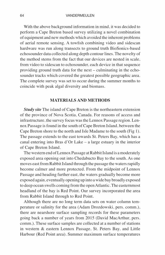
Study site The island of Cape Breton is the northeastern extension of the province of Nova Scotia, Canada. For reasons of access and infrastructure, the survey focus was the Lennox Passage region. Len-nox Passage is found in the south of Cape Breton Island, between the Cape Breton shore to the north and Isle Madame to the south (Fig 1). The passage extends to the east towards St. Peters Bay, which has a canal entering into Bras d’Or Lake – a large estuary in the interior of Cape Breton Island.

The western end of Lennox Passage at Rabbit Island is a moderately exposed area opening out into Chedabucto Bay to the south. As one moves east from Rabbit Island through the passage the waters rapidly become calmer and more protected. From the midpoint of Lennox Passage and heading further east, the waters gradually become more exposed again, eventually opening up into a wide bay broadly exposed to deep ocean swells coming from the open Atlantic. The easternmost headland of the bay is Red Point. Our survey incorporated the area from Rabbit Island through to Red Point.

Although there are no long term data sets on water column tem-perature or salinity for the area (Adam Drozdowski, pers. comm.), there are nearshore surface sampling records for these parameters going back a number of years from 2015 (David MacArthur, pers. comm.). These surface samples are collected at a number of stations in western & eastern Lennox Passage, St. Peters Bay, and Little Harbour (Red Point area). Summer maximum surface temperatures


at these stations can reach 23°C, while salinity ranges from 0 to 37 ppt depending upon freshwater inputs (David MacArthur, pers. comm.). There is variable ice cover in Lennox Passage during the winter months.

Towfish survey A novel towfish was deployed as described in Vandermeulen (2011a, 2013, 2014b). Briefly, the towfish consisted of a video camera with 10 cm laser scale and a 330 kHz sidescan sonar set to a 30 m swath width. The video feed was used to ground truth the sidescan imagery in real time. The towfish was positioned to sub-meter precision via a transponder / transceiver system coupled to a high end dGPS with Canadian Coast Guard beacon correc-tion. During the survey, the towfish was hauled behind the vessel from depth to the shallows on transects perpendicular to shore. Some transects were run from shore to an opposite shore. The ves-sel speed over ground during transect runs was approximately 1.5 knots. The towfish was held approximately 30 cm off the bottom at all times. In this position, the field of view of the camera was ap-proximately 1 m.

Fig 1 The study area. The provinces of New Brunswick (NB), Prince Edward Island (PEI), and Nova Scotia (NS) with its Cape Breton Island region (CB) including Bras d’Or Lake (BL). Inset: Ilse Madame (IM), Rabbit Island (RI), Lennox Passage (LP), St. Peters Bay (SPB), and Red Point (RP).

VANDERMEULEN66

The survey area was divided into six zones, with at least two tran-sects per zone (Fig 2). The zones were chosen to reflect differences in depth and exposure within the survey area. Zone 1 was moderately exposed with depths to just over 10m with a water surface area of approximately 12 km²; Zones 2 and 3 were much more protected and shallower (approximately 9 and 7 km², respectively); Zone 4 was a transition area where Lennox Passage widened and became deeper (>10m) and more exposed, with a surface area of 22 km²; Zone 5 was a broad exposed area with depths >20m and a surface area of approximately 37 km²; and Zone 6 was a large, deep open bay with extreme exposure (large swells from the open Atlantic). Its water surface area was approximately 52 km².

Post processing of towfish data was accomplished via the use of specialized commercial software (Vandermeulen 2011a). A MapInfo GIS project was created with a hydrographic chart background layer in which sidescan GeoTIFF images, towfish track positions (which were updated every 1.3 seconds) and AVI video clips were embedded. Each video clip was approximately 10 min long and embedded into its starting point on the associated GeoTIFF image. In this manner, each transect was assigned a number and then divided into sections defined by the associated video clips. For example, transect number

Fig 2 The survey area divided into six zones (numbers in rectangles). The towfish transects are indicated by numbers in circles.


3 in the section covered by video clip number 5 would be coded as T3S5. By examining the sidescan imagery in a particular section of the transect and comparing it to the video clip for that section, it was possible to classify bottom types and macrophyte types associated with each towfish track position. The resulting towfish based classifica-tion was used to ground truth the echosounder survey that followed.

Echosounder survey Independently of the towfish transects, an echosounder system was deployed as described in Vandermeulen (2011b). The BioSonics Inc. (Seattle, WA 98107) system consisted of a DT-X digital echosounder surface unit, a 210 kHz single beam digital transducer with 6° cone angle, and a 430 kHz single beam digital transducer with 6° cone angle and built in heading / pitch / roll (HPR) sensor. The transducers were chosen for their ability to detect bottom type and macrophyte cover, respectively. Both transducers operated at the same time, with alternating ping cycles. The echosounder track was recorded to sub-meter precision via the same dGPS unit used for the towfish. During the survey, hydrographic chart contour lines were followed to get relatively uniform sized ping foot prints for better precision in later data analyses (Vandermeulen 2011b). The vessel speed over ground was approximately 4 knots, similar to Sabol et al. (2009). In order to maximize the ability to pick out different types of algal assemblages, 5, 10 and 20 m contour lines were chosen for this survey.

Data processing was accomplished via specialized software from BioSonics, Inc. (Vandermeulen 2011b). Visual Bottom Typer™ was applied to the 210 kHz dataset to sort and cluster acoustic bottom sig-natures into groups of bottom types (e.g. hard versus soft). EcoSAV™ was used on the 430 kHz dataset to create bins of macrophyte canopy heights. Later on, both datasets were revisited with Visual Habitat™ software, an update incorporating and enhancing the properties of the previous two software packages.

Quadrat survey Data from the towfish and echosounder surveys was extracted to determine sites for SCUBA based destructive sam-pling for standing stock data on dominant algal species. An effort was made to select representative algal communities at 5, 10 and 20 m depths along towfish transects based upon the video data. The survey design was not random; it was an attempt to discern areas with notable algal cover. The survey effort was divided into the three depths plus shore stations in order to maximize the ability to explore different types of algal communities.

VANDERMEULEN68

One m2 and 0.25 m2 quadrats were constructed from aluminum angle, and paint scrapers were used to remove all algae within each quadrat at each sampling station. A slurp gun was used to remove delicate algal forms which could not easily be stuffed into a collec-tion bag after scraping (Vandermeulen et al. 2011). Three quadrats of equal size were used at each sampling station. The quadrats were deliberately placed by the divers to obtain a representative sample of the attached algal flora in the immediate area. Material from each quadrat was placed into individually labelled sampling bags, repackaged in the dive boat and placed into coolers for transport. That same evening, the algal samples were spun in a mesh bag or in a salad spinner to remove surface moisture. Material from each quadrat was sorted by species and a wet weight per species was obtained. Rare species, where wet weight was less than 1 g, were ignored. The weight of epiphytes was also ignored; the epiphyte load was light in any case. In some instances, subsamples were preserved in formalin and taken back to the lab for later sorting and weighing or to confirm identification. Average weights were calculated from the three quadrats for each algal species at each station.

RESULTS

Species list The algal and other macrophytic species found during this study

are listed in Table 1. Unless multiple species were present in a genus, species are referred to by generic name alone.

Towfish surveyThe survey ran from June 8-10, 2010. Sixteen transects were com-

pleted, covering a total distance of approximately 26 km and a total zonal surface area of approximately 140 km² (Fig 2). Fig 3 provides an example of bottom type results at the north end of transect 1 (T1), with the shoreline indicated in tan color at the top of the figure. The hydrographic chart background is useful for interpreting the towfish data. Note how our vessel was able to obtain sidescan and video data in waters <1m deep. In this example, the substrate tran-sitions from a soft muddy bottom (low acoustic reflectivity, dark brown sidescan image) into a coarse gravel bottom (high acoustic reflectivity, light ‘brassy’ sidescan image) at a depth of about 10 m from Canadian Chart Datum (essentially a point below which the


Table 1 Species list of algal and other macrophytic species found during the seaweed survey.

TaxonAgarum clathratum DumortierAhnfeltia plicata (Hudson) FriesAntithamnionella floccosa (O.F. Müller) WhittickAscophyllum nodosum (L.) Le JolisBonnemaisonia hamifera HariotCallithamnion spp.Callophyllis cristata (C. Agardh) KützingCeramium virgatum RothChondrus crispus StackhouseChorda filum (L.) StackhouseChordaria flagelliformis (O.F. Müller) C. AgardhCorallina officinalis L.Cystoclonium purpureum (Hudson) BattersDesmarestia aculeata (L.) J.V. LamourouxDesmarestia viridis (O.F. Müller) J.V. LamourouxDictyosiphon foeniculaceus (Hudson) GrevilleDilsea integra (Kjellman) RosenvingeEctocarpus spp.Fucus distichus L.Fucus serratus L.Fucus vesiculosus L.Furcellaria lumbricalis (Hudson) J.V. LamourouxGracilaria sp.Halosiphon tomentosus (Lyngbye) JaasundLaminaria digitata (Hudson) J.V. LamourouxNeosiphonia harveyi (J.W. Bailey) M.-S. Kim, H.-G. Choi, M. Guiry & G.W. SaundersOdonthalia dentata (L.) LyngbyePalmaria palmata (L.) Weber & MohrPhycodrys rubens (L.) BattersPhyllophora spp.Polysiphonia fucoides (Hudson) GrevillePtilota serrata KützingRhodomela confervoides (Hudson) P.C. SilvaSaccharina groenlandica (Rosenvinge) C.E. Lane, C. Mayes, L. Druehl & G.W. SaundersSaccharina latissima (L.) C.E. Lane, C. Mayes, L. Druehl & G.W. SaundersSphacelaria spp.Zostera marina L.

tide rarely falls). The sidescan imagery was ground truthed via the associated video clips to generate the bottom classification seen in the midline of the transect. The midline represents the actual position of the towfish during the haul, and each colored symbol is a towfish position data point generated by the towfish transponder / transceiver system. The macrophyte classification for this same portion of the bottom is shown in Fig 4. As would be expected, the deeper soft muddy bottom has no macrophytes while Saccharina grew on the coarse gravel bottom in its deeper portion with Fucus in the shallows.

VANDERMEULEN70

A thin band of Zostera was also seen in the shallows on the gravel. Different bottom types were recognizable with the sidescan imagery

(Fig 5). A dark, featureless sidescan image indicates a soft bottom of low acoustic reflectivity (Fig 5a). The two bright bands on either side of the sidescan image are artifacts. Figure 5b demonstrates the much higher acoustic reflectivity of coarse sand, resulting in a much brighter image which is also relatively flat and featureless (there are a couple of larger boulders in the lower left of the image, note the long dark acoustic ‘shadows’ they create). A bright image with more ‘texture’ or features is seen in Fig 5c, constituting a gravel base with

Fig 3 Typical results of towfish bottom type data embedded into the GIS. Sidescan image with bottom classification in mid-line (olive circles = soft sediment; blue stars = coarse gravel; the red chevron indicates the direction of the towfish haul and the position of the associated video clip). The width of the sidescan image is 30m. Transect T1.

Fig 4 The same towfish track as Fig 3 with the macrophyte classification (light blue circles = 100% bare substrate; green = Saccharina dominated; red = Fucus dominated; dark blue = Zostera dominated).


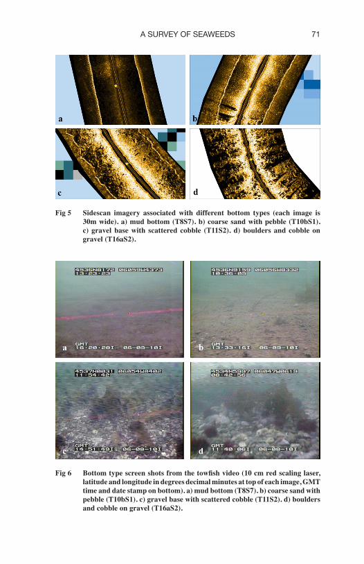
Fig 5 Sidescan imagery associated with different bottom types (each image is 30m wide). a) mud bottom (T8S7). b) coarse sand with pebble (T10bS1). c) gravel base with scattered cobble (T11S2). d) boulders and cobble on gravel (T16aS2).

Fig 6 Bottom type screen shots from the towfish video (10 cm red scaling laser, latitude and longitude in degrees decimal minutes at top of each image, GMT time and date stamp on bottom). a) mud bottom (T8S7). b) coarse sand with pebble (T10bS1). c) gravel base with scattered cobble (T11S2). d) boulders and cobble on gravel (T16aS2).

VANDERMEULEN72

scattered mid-sized cobble (note the numerous small acoustic shad-ows). The greatest amount of texture is seen on boulder / cobble bot-toms, with many long acoustic shadows covering the image (Fig 5d). All bottom types indicated by the sidescan imagery were confirmed by the associated video at the same location (Fig 6). It was also possible to identify different groups of macrophytes via the video feed (Fig 7).

The video and sidescan information from the towfish was used to create both a bottom classification (Table 2) and a macrophyte or canopy classification (Table 3). The canopy classification shown in Table 3 was driven by an attempt to find associations of algae where one species would dominate with a cover of ≥ 50%. In deeper areas

Fig 7 Macrophyte screen shots from the towfish video. a) eelgrass, Z. marina (T4S4). b) F. serratus (T10bS3). c) L. digitata (T13S2). d) S. latissima (T13S2). e) Desmarestia (T13S2). f) Agarum (T16aS2).


with many bare patches of substrate, Agarum would occasionally dominate as the main algal species but it’s cover did not approach 50%. However, Agarum and its assemblage of species did constitute a valid canopy class and was given a canopy code of four (Table 3). The term ‘crozier morph’ has been associated with the taxon Laminaria longicruris Bachelot de la Pylaie in the past (Sears 2002). It refers here to thalli of S. latissima with elongated stipes of various degrees of inflation (Chapman 1973, 1974).

The towfish survey data were used to create 22,915 ground truth point records based upon latitude and longitude of the towfish at each 1.3 s time stamp with bottom type plus canopy codes at each of those towfish positions. The towfish ground truth point records were used to derive the proportion of bottom types recorded by towfish

Table 2 Towfish bottom classification codes.

Code Type

1 soft (mud / silt)2 hard (sand / silt)3 hard (coarse gravel with occasional cobble)4 hard (cobble on sand base)5 hard (boulder / reef)

Table 3 Towfish canopy classification codes.

Code Type

1 Fucus dominant (cover ≥ 50%) – mostly F. serratus; may have some Chorda / Halosiphon, Saccharina, red algal turf or bare patches; Zostera cover can be up to 50% at some shallow locations

2 Saccharina dominant (cover ≥ 50%) – mostly crozier morph of S. latissima (T13 had L. digitata mixed in); may have some Fucus, Agarum, Desmarestia, red algal turf or bare patches

3 Zostera dominant (cover ≥ 50% as a ‘meadow’, more extensive than a col-lection of patches) – may have some Fucus, Chorda / Halosiphon, variety of other seaweeds, or bare patches

4 Agarum dominant (cover ≥ 40%) – usually in deeper areas with many bare patches, may have some Saccharina, Desmarestia or red algal turf (Ptilota)

5 70% bare – may have some algal turf (green, brown or red), Zostera, Chorda / Halosiphon, Saccharina, Desmarestia, Agarum, or drift material

6 100% bare – no consistent macrophyte cover; may have some algal mats, organic debris, or drift material

7 Desmarestia dominant (cover ≥ 50%) – may have some Saccharina, Agarum, bare patches or drift material

8 red algal coralline crust on boulders at depth (cover ≥ 50%) – may have some Agarum, Desmarestia, or sea urchins; upright coralline thalli rare

VANDERMEULEN74

Tabl

e 4

To

wfis

h bo

ttom

type

dat

a by

zon

e.

Zon

e C

ount

for

bott

om

Cou

nt fo

r bo

ttom

C

ount

for

bott

om

Cou

nt fo

r bo

ttom

C

ount

for

bott

om

Tota

l by

ty

pe #

1 (%

) ty

pe #

2 (%

) ty

pe #

3 (%

) ty

pe #

4 (%

) ty

pe #

5 (%

) zo

ne

1 29

10 (7

6.5)

38

(1.0

) 75

0 (1

9.7)

10

6 (2

.8)

0 (0

.0)

3804

2 19

21 (7

6.3)

0

(0.0

) 59

6 (2

3.7)

0

(0.0

) 0

(0.0

) 25

173

2205

(99.

5)

0 (0

.0)

11 (0

.5)

0 (0

.0)

0 (0

.0)

2216

4 37

15 (6

1.5)

23

6 (3

.9)

2010

(33.

3)

79 (1

.3)

0 (0

.0)

6040

5 12

01 (2

1.6)

87

7 (1

5.8)

22

13 (3

9.8)

0

(0.0

) 12

64 (2

2.8)

55

556

0 (0

.0)

943

(33.

9)

1350

(48.

5)

150

(5.4

) 34

0 (1

2.2)

27

83To

tals

11

952

2094

69

30

335

1604

22

915

Tabl

e 5

To

wfis

h ca

nopy

type

dat

a by

zon

e.

Zon

e C

ount

C

ount

C

ount

C

ount

C

ount

C

ount

C

ount

C

ount

To

tal

ca

nopy

type

ca

nopy

type

ca

nopy

type

ca

nopy

type

ca

nopy

type

ca

nopy

type

ca

nopy

type

ca

nopy

type

zo

ne

#1

(%)

#2 (%

) #3

(%)

#4 (%

) #5

(%)

#6 (%

) #7

(%)

#8 (%

)

1 20

4 (5

.4)

212

(5.6

) 32

(0.8

) 0

(0.0

) 21

7 (5

.7)

3139

(82.

5)

0 (0

.0)

0 (0

.0)

3804

2 43

(1.7

) 16

2 (6

.4)

33 (1

.3)

0 (0

.0)

123

(4.9

) 21

56 (8

5.7)

0

(0.0

) 0

(0.0

) 25

173

11 (0

.5)

0 (0

.0)

57 (2

.6)

0 (0

.0)

0 (0

.0)

2148

(97.

0)

0 (0

.0)

0 (0

.0)

2216

4 28

3 (4

.7)

856

(14.

2)

226

(3.7

) 11

(0.2

) 21

6 (3

.6)

4263

(70.

6)

185

(3.1

) 0

(0.0

) 60

405

970

(17.

5)

1666

(30.

0)

257

(4.6

) 38

(0.7

) 11

6 (2

.1)

2073

(37.

3)

152

(2.7

) 28

3 (5

.1)

5555

6 0

(0.0

) 34

(1.2

) 0

(0.0

) 97

6 (3

5.1)

56

2 (2

0.2)

12

11 (4

3.5)

0

(0.0

) 0

(0.0

) 27

83To

tals

15

11

2930

60

5 10

25

1234

14

990

337

283

2291

5


survey zone, not binned by depth. The resulting summary (Table 4) provides a general overview of bottom types which are consistent with the hydrography of each zone. For example, zones 1 – 4 were the more sheltered zones of the survey and they were dominated by soft mud / silt (bottom type #1) with no hard boulder / reef areas (bottom type #5) and very little or no hard sand / silt areas (bottom type #2). Zone 5 was a transitional area depth and exposure wise, and it had a relatively even proportion of each of the bottom types (Table 4). Zone 6 had the greatest depth and exposure, and no soft bottoms were recorded by the towfish in that zone.

Table 5 is a summary of the proportion of canopy types in each towfish survey zone, also not binned by depth. Once again, the results are consistent with the hydrography of each zone. The zone with the most even proportions of all bottom types also had the most even proportions of all canopy types, Zone 5. It was also the only zone not missing any canopy types. Zones 1 – 3 were notable for their relative absence of macrophytes, having no consistent macrophyte cover over 80% of the time (canopy type #6). This is reasonable, considering that >76% of the surveyed bottom in these zones was soft mud or silt (Table 4). Zone 6 was the only zone missing Zostera (canopy type #3), consistent with the high degree of wave exposure in the zone. Agarum (canopy type #4) was the dominant macrophyte in Zone 6. There was also a considerable amount of completely or partially bare bottom, as would be expected for the overall greater depths found in Zone 6.

Echosounder survey The survey was completed during June 21-24, 2010. The tracks of

the echosounder data acquisition are indicated in Fig 8. A corrupted data file led to a gap in coverage on the 10m contour in the middle of Zone 4. A total of approximately 80 km of coastline was covered by the survey.

Both Visual Bottom Typer™ and EcoSAV™ software packages are loaded with echogram files, parameters are set for analysis, and data processing occurs in a batch mode. If the results from these packages seem odd or inconsistent with towfish ground truth data, the operator must reset the parameters based upon experience or other opinions as to what might improve the results. Although the results from Visual Bottom Typer™ and EcoSAV™ on the 210 and 430 kHz datasets were reasonably consistent with the towfish ground

VANDERMEULEN76

truth data, a decision was made to revisit both datasets with more recent and updated Visual Habitat™ (VH) software.

The value of the VH software is the ability to edit echograms. The software selects bottom detection and macrophyte detection lines automatically, and these lines can be edited (Fig 9). Editing allows for the correction of errors in the creation of the original detection lines such as false positives for a macrophyte canopy. Softer bottoms oc-casionally generate these false positives and they are easily recognized in the echograms. After editing, VH can process the echograms to detect different types of acoustic signatures associated with different bottom types, or estimate the canopy height of macrophyte cover. In other words, VH includes the functions of both Visual Bottom Typer™ and EcoSAV™ in one software package.

After some experimentation with VH , it was determined that setting the software to search for six types / classes of acoustic signatures to associate with different bottom types provided quite robust results for comparison to towfish ground truth data. Similarly, binning the canopy height results into three different categories seemed most satisfactory.

Fig 8 The survey area indicating the tracks of the echosounder data acquisition. The tracks followed three different depth contour lines, 5m (red), 10m (green), and 20m (blue).


Echosounder ground truthing was obtained by examining cross points with towfish transects. Vandermeulen et al. (2017) explain this process and provide raw data tables of results. This can be illustrated by towfish transect T7 where it was crossed by a pass of the echosounder along the 10 m contour line (Figs 10 & 11). Essentially, this was an empirical process to check if the echosounder based VH classification matched the towfish classification at each cross point for both bottom type and macrophyte cover. The VH classifications were color coded in the GIS to match the towfish classifications as closely as possible. Table 6 provides the results for the VH bottom type classification.

The echosounder data and associated VH bottom classification analysis provided a mechanism to examine bottom types by zone and depth (Table 7). The proportion of unclassified (or clear) points in the GIS ranged from 10.5 to 56.3% – so an interpretation of this analysis is tentative at best. However, the general patterns of hard versus soft bottom identified by the analysis do seem logical. At the 5 m depth contour, Zone 6 had the highest proportion of hard versus soft bottom (proportion of blue versus red points in the GIS). This is consistent with the high degree of wave exposure in Zone 6. Zones 1 and 5 also had a relatively higher proportion of hard bottom at

Fig 9 Screen shot of VH bottom detection line (orange arrow) and macrophyte detection line (green arrow). The light green region between these two lines represents the macrophyte canopy.

VANDERMEULEN78

Fig 10 VH bottom classification crossing north end of towfish transect T7 near the 10m contour line. The towfish bottom classification (coarse gravel, blue stars) matches the VH classification (coarse gravel / sand or silt, blue circles) at the cross point.

Fig 11 Ground truthing for VH macrophyte canopy classification. Same location as Fig 10. The towfish classification (Saccharina, green circles) is consistent with the VH canopy height classification of 0.5 to <1.6m at the cross point (green circles). Canopy height was slightly lower on either side of the cross point (yellow circles, 0.2 to <0.5m) but still consistent with a signal from a larger algal thallus.


the 5 m depth contour, matching their exposure regime relative to Zone 6. At the 10 m depth contour, Zone 6 continued to have a very high ratio of hard to soft bottom – a pattern followed by Zone 5. Although the data for the 20 m depth contour were limited (Vander- meulen et al. 2017), it was interesting to see that Zone 6 was domi-nated by a rugose or textured bottom (many blue colored dots in the GIS) consistent with the coarse gravel or boulders seen in that area.

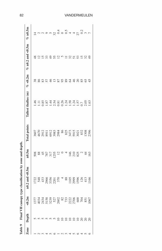
Towfish data were also used to ground truth VH canopy analy-ses. Details are provided in Vandermeulen et al. (2017) and the summary results for all depth contours are seen in Table 8. A sum-mary of canopy type classification by zone and depth is provided in Table 9. These results are consistent with the bottom type classifica-tion summarized in Table 7. For example, those zones and depths with greater than 80% of canopy in bin height <0.2 m (essentially no macrophyte cover) in Table 9 are also the zones and depths with a ‘blue to red’ ratio of <1 in Table 7. In other words, areas with little or no macrophyte cover are also dominated by softer sedi-ments or relatively featureless bottoms with little relief. Conversely, those areas with over 50% of canopy in bin height >0.2 m (areas with a substantial amount of macrophyte cover) in Table 9 are also the zones and depths with a ‘blue to red’ ratio of >4 in Table 7. Areas with hard and textured bottoms had a greater macrophyte canopy.

Quadrat surveyThe quadrat survey ran from July 10-14, 2010. Fig 12 provides

the location of the various sampling stations. More detailed station descriptions are available in Vandermeulen et al. (2017). Station B – 2 was selected on the basis of echosounder information. The echogram at the 5 m contour in this area indicated large algae with lacunae,

Table 6 Color coded VH bottom classifications in GIS.

Depth (m) Description Color code

5 ‘soft’ red5 ‘hard’ blue5 undetermined clear10 ‘soft’ red10 ‘hard’ blue10 undetermined clear20 ‘flat’ or featureless sediment of varying hardness red20 ‘hard or textured’ blue20 undetermined clear

VANDERMEULEN80

Tabl

e 7

Sum

mar

y V

H b

otto

m ty

pe c

lass

ifica

tion

by z

one

and

dept

h (G

IS p

oint

s col

or c

oded

cle

ar, r

ed a

nd b

lue)

.

Zon

e de

pth

clea

r re

d bl

ue

tota

l %

cle

ar

% r

ed

% b

lue

tota

l %

Blu

e : r

ed

1 5

966

522

2089

35

77

27.0

0587

14

.593

23

58.4

0089

10

0 4.

0019

162

5 13

68

1755

15

46

4669

29

.299

64

37.5

8835

33

.112

02

100

0.88

0912

3 5

780

1577

55

4 29

11

26.7

9492

54

.173

82

19.0

3126

10

0 0.

3513

4 5

2358

30

16

3536

89

10

26.4

6465

33

.849

61

39.6

8575

10

0 1.

1724

145

5 17

46

886

4280

69

12

25.2

6042

12

.818

29

61.9

213

100

4.83

076

5 60

2 90

32

91

3983

15

.114

24

2.25

9603

82

.626

16

100

36.5

6667

1 10

16

81

853

451

2985

56

.314

91

28.5

7621

15

.108

88

100

0.52

8722

2 10

45

39

1

85

52.9

4118

45

.882

35

1.17

6471

10

0 0.

0256

413

10

168

332

325

825

20.3

6364

40

.242

42

39.3

9394

10

0 0.

9789

164

10

1007

11

29

1338

34

74

28.9

8676

32

.498

56

38.5

1468

10

0 1.

1851

25

10

1803

32

0 37

91

5914

30

.486

98

5.41

0889

64

.102

13

100

11.8

4688

6 10

47

7 30

25

14

3021

15

.789

47

0.99

3049

83

.217

48

100

83.8

4 20

87

64

1 10

4 83

2 10

.456

73

77.0

4327

12

.5

100

0.16

2246

5 20

21

0 42

8 67

0 13

08

16.0

5505

32

.721

71

51.2

2324

10

0 1.

5654

216

20

861

129

1406

23

96

35.9

3489

5.

3839

73

58.6

8114

10

0 10

.899

22


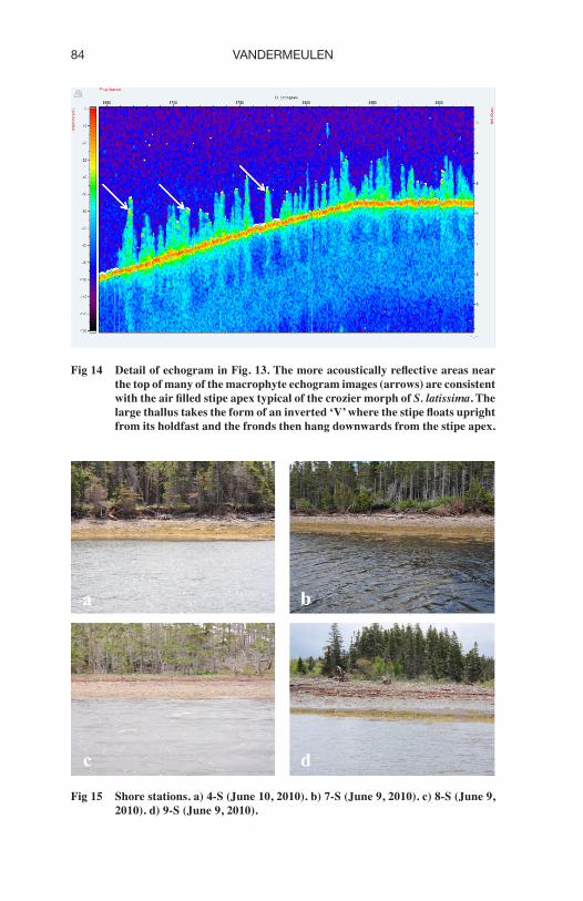
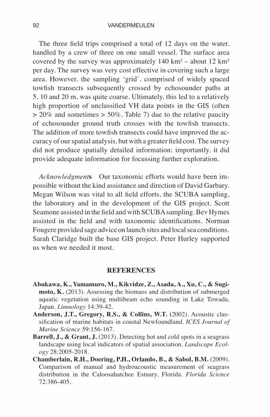
most likely the crozier morph of S. latissima with an inflated stipe (Figs 13 & 14). Images of the shore stations are shown in Fig 15.

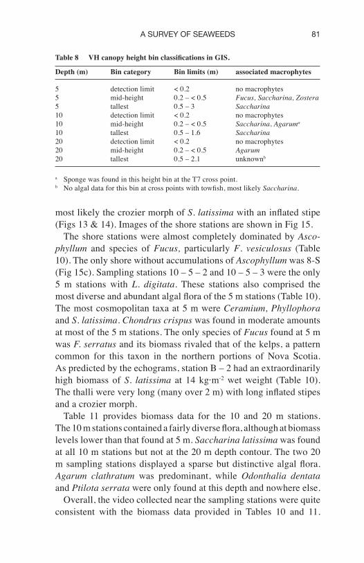
The shore stations were almost completely dominated by Asco-phyllum and species of Fucus, particularly F. vesiculosus (Table 10). The only shore without accumulations of Ascophyllum was 8-S (Fig 15c). Sampling stations 10 – 5 – 2 and 10 – 5 – 3 were the only 5 m stations with L. digitata. These stations also comprised the most diverse and abundant algal flora of the 5 m stations (Table 10). The most cosmopolitan taxa at 5 m were Ceramium, Phyllophora and S. latissima. Chondrus crispus was found in moderate amounts at most of the 5 m stations. The only species of Fucus found at 5 m was F. serratus and its biomass rivaled that of the kelps, a pattern common for this taxon in the northern portions of Nova Scotia. As predicted by the echograms, station B – 2 had an extraordinarily high biomass of S. latissima at 14 kg·m-2 wet weight (Table 10). The thalli were very long (many over 2 m) with long inflated stipes and a crozier morph.

Table 11 provides biomass data for the 10 and 20 m stations. The 10 m stations contained a fairly diverse flora, although at biomass levels lower than that found at 5 m. Saccharina latissima was found at all 10 m stations but not at the 20 m depth contour. The two 20 m sampling stations displayed a sparse but distinctive algal flora. Agarum clathratum was predominant, while Odonthalia dentata and Ptilota serrata were only found at this depth and nowhere else.

Overall, the video collected near the sampling stations were quite consistent with the biomass data provided in Tables 10 and 11.

Table 8 VH canopy height bin classifications in GIS.

Depth (m) Bin category Bin limits (m) associated macrophytes

5 detection limit < 0.2 no macrophytes5 mid-height 0.2 – < 0.5 Fucus, Saccharina, Zostera5 tallest 0.5 – 3 Saccharina10 detection limit < 0.2 no macrophytes10 mid-height 0.2 – < 0.5 Saccharina, Agaruma

10 tallest 0.5 – 1.6 Saccharina20 detection limit < 0.2 no macrophytes20 mid-height 0.2 – < 0.5 Agarum20 tallest 0.5 – 2.1 unknownb

a Sponge was found in this height bin at the T7 cross point.b No algal data for this bin at cross points with towfish, most likely Saccharina.

VANDERMEULEN82

Tabl

e 9

Fina

l VH

can

opy

type

cla

ssifi

catio

n by

zon

e an

d de

pth.

Zon

e D

epth

<0

.2m

≥0

.2 a

nd <

0.5m

≥0

.5m

To

tal p

oint

s Ta

llest

thal

lus (

m)

% <

0.2m

%

≥0.

2 an

d <0

.5m

%

≥0.

5m

1 5

1377

17

22

508

3607

1.

46

38

48

142

5 40

34

548

88

4670

1.

11

86

12

23

5 24

34

433

45

2912

0.

85

83

15

24

5 51

58

2966

78

7 89

11

1.87

57

33

9

5 5

3239

33

56

317

6912

1.

44

46

49

56

5 52

7 22

01

1255

39

83

2.54

13

55

32

1 10

26

02

370

12

2984

0.

81

87

12

0.4

2 10

82

4

0 86

0.

26

95

5 0

3 10

73

3 88

4

825

1.24

89

11

0.

54

10

2222

11

05

146

3473

1.

58

64

32

45

10

2706

29

99

210

5915

1.

24

46

51

46

10

600

1596

82

5 30

21

1.57

20

53

27

4 20

70

4 12

6 2

832

0.7

85

15

0.2

5 20

85

1 41

3 44

13

08

2.05

65

32

3

6 20

10

67

1166

16

3 23

96

1.63

45

49

7


Fig 12 Sampling stations. The coding is transect number-depth-sample number.

Fig 13 Echogram indicating large thalli of S. latissima with crozier morph at station B-2. The range scale on the right indicates that many of these thalli are close to 2m tall.

VANDERMEULEN84

Fig 15 Shore stations. a) 4-S (June 10, 2010). b) 7-S (June 9, 2010). c) 8-S (June 9, 2010). d) 9-S (June 9, 2010).

Fig 14 Detail of echogram in Fig. 13. The more acoustically reflective areas near the top of many of the macrophyte echogram images (arrows) are consistent with the air filled stipe apex typical of the crozier morph of S. latissima. The large thallus takes the form of an inverted ‘V’ where the stipe floats upright from its holdfast and the fronds then hang downwards from the stipe apex.


Tabl

e 10

B

iom

ass d

ata

(wet

wei

ght g

·m-2) f

or sh

ore

and

5 m

sam

plin

g st

atio

ns.

Taxo

n

Sa

mpl

ing

Stat

ion

ID#

4-

S 7-

S 8-

S 9-

S 2-

5-2

3-5-

1 B

-2

9-5-

4 10

-5-2

10

-5-3

12

-5-2

14

-5-4

Ahnf

eltia

68

A. n

odos

um

2200

14

000

19

00

B.

ham

ifera

2

00

C. c

rist

ata

7

.6

11

Cer

amiu

m sp

p.a

31

26

23

390

2.7

6.

4

43C

. cri

spus

44

56

11

1

30

87

Cho

rdar

ia sp

.

5

.3

C

oral

lina

sp.

73

9

.3

95

C. p

urpu

reum

5

.8

25

21

80

Des

mar

estia

spp.

b

40

21

59

Dic

tyos

ipho

n sp

.

2.2

D

. int

egra

100

Ecto

carp

us sp

.

38

F. d

istic

hus

2

00

F.

serr

atus

42

00

3

60

200

3100

160

18

00

2300

F. v

esic

ulos

us

670

3

000

1600

43

00

F.

lum

bric

alis

4

60

86

2

.7

73

62

500

L.

dig

itata

22

00

900

P. p

alm

ata

27

2

70

6

.7

5.3

P. ru

bens

20

22

Phyl

loph

ora

sp.

37

1

40

7

6

29

1100

4

10

100

92Po

lysi

phon

ia sp

p.c

42

14

16

0 6

30

110

4.0

VANDERMEULEN86

Rhod

omel

a sp

.d

5

.3

6

.3

28

29

S. la

tissi

mae

2300

67

00

1400

0

2.7

73

1200

5

00

80

Spha

cela

ria

sp.

5

.6a

Mos

t com

mon

ly C

. virg

atum

, occ

asio

nally

tang

led

in w

ith sm

all a

mou

nts o

f Pol

ysip

honi

a sp

p., C

allit

ham

nion

sp. o

r B. h

amife

ra.

b A

n al

mos

t equ

al m

ix o

f D. a

cule

ata

and

D. v

irid

is, p

lus s

ampl

es n

ot id

entifi

able

to sp

ecie

s.c

An

alm

ost e

qual

mix

of P

. fuc

oide

s and

N. h

arve

yi, p

lus a

few

sam

ples

not

iden

tifiab

le to

spec

ies.

d M

ost s

ampl

es n

ot id

entifi

able

to sp

ecie

s, bu

t a c

oupl

e se

en a

s R. c

onfe

rvoi

des

e A

n al

mos

t equ

al m

ix o

f the

shor

t stip

e m

orph

with

frill

y bl

ade

and

the

long

stip

e m

orph

. B-2

with

larg

e lo

ng st

ipe

plan

ts w

ith c

rozi

er m

orph

and

hype

r-in

flate

d st

ipe.

Man

y of

the

plan

ts u

nder

this

taxo

n m

ay a

ctua

lly b

e S.

gro

enla

ndic

a (S

aund

ers p

ers.

com

m.).

Tabl

e 10

C

ont'd

Taxo

n

Sa

mpl

ing

Stat

ion

ID#

4-

S 7-

S 8-

S 9-

S 2-

5-2

3-5-

1 B

-2

9-5-

4 10

-5-2

10

-5-3

12

-5-2

14

-5-4


Tabl

e 11

B

iom

ass d

ata

(wet

wei

ght g

·m-2

) for

10

and

20 m

sam

plin

g st

atio

ns.

Taxo

n

Sa

mpl

ing

Stat

ion

ID#

1-

10-1

2-

10-1

7-

10-1

11

-10-

2 13

-10-

1 11

-20-

1 13

-20-

1

A. c

lath

ratu

m

35

00

89An

titha

mni

onel

la sp

.

69

C. c

rist

ata

2.4

5.0

Cer

amiu

m sp

p.

39

6.7

17

C

. cri

spus

16

0

4.

0

C

hord

aria

sp.

16

C

oral

lina

sp.

130

C

. pur

pure

um

4.

0 6.

7 19

0

D

esm

ares

tia sp

p.

93

16

00

110

D. i

nteg

ra

9.

3 Ec

toca

rpus

sp.

23

F.

ves

icul

osus

61

F. lu

mbr

ical

is

180

100

Gra

cila

ria

sp.

13

0

O

. den

tata

11

4.0

P. p

alm

ata

11

6.7

11

12

P. r

uben

s

36

12Ph

yllo

phor

a sp

. 96

68

4.

0

15

5.

3Po

lysi

phon

ia sp

p.

54

190

60

530

74P.

ser

rata

8.0

11Rh

odom

ela

sp.

5.7

16

40

S.

latis

sim

a 41

00

3400

95

0 44

00

2700

VANDERMEULEN88

Dominant algal taxa in the video tended to dominate biomass in the destructive quadrat samples.

DISCUSSION

Algal communities in the survey areaThe abundance and diversity of algae observed in the study area

was strongly related to the depth, diversity and abundance of bottom types in each zone. Zones 1 – 3 were relatively shallow and shel-tered and were dominated by soft mud / silt (towfish data, Table 4). Towfish data also indicated over 80% of the bottom in these zones had no consistent macrophyte cover (Table 5). The echosounder data (Table 7) are consistent with the towfish data in this regard. The echosounder data were stratified by depth and indicated that of the three zones, only Zone 1 had moderate amounts of hard substrata and these only occurred in relative abundance at the 5 m depth contour. Zone 1 at 5 m depth was also the only location in these three zones with a relative abundance of taller canopy (Table 9), indicating kelps. Zone 4 was similar to the first three zones in terms of its shallow depths but it had slightly more hard substrate (Table 4). All four of these relatively shallow protected zones had limited algal or seagrass cover, usually less than 10% each of Fucus, Saccharina or Zostera dominated cover in the towfish transects (Table 5). Zone 4 also had small amounts of Agarum and Desmarestia (Table 5).

Zone 5 was a transitional area, deeper and with a greater variety of bottom types relative to the first four zones (towfish data, Table 4). Zone 5 also had the most even proportions of all canopy types and was the only zone not missing any canopy types (Table 5). This zone had the highest proportion of Saccharina dominated canopy at 30% (towfish data, Table 5). The echosounder data indicated that Zone 5 was also dominated by hard substrata at 5 m and 10 m depth (Table 7). Zone 5 also consistently had a detectable algal canopy of over 50% of classified VH data points at 5 and 10 m (Table 9). Of the first five zones, only Zone 1 at 5 m depth had similar algal cover (Table 9).

Zone 6 was the deepest and most exposed of all zones, with no soft bottoms recorded by the towfish (Table 4). Consistent with the greater depths of Zone 6, there was a considerable amount of com-pletely or partially bare bottom and the dominant alga was Agarum


(towfish data, Table 5). The echosounder data confirmed the very high proportion of hard bottom at all depths in Zone 6 (Table 7). Zone 6 had the highest proportion of detectable canopy in the VH analysis, with 80% or more of data points at 5 and 10 m indicating algal cover and over 50% algal cover even at 20 m (Table 9). A relatively high proportion of these data points at 5 and 10 m were for a canopy height of ≥ 0.5 m, indicating kelps.

Previous algal surveys in the study areaThe study area was impacted by the “Arrow” Bunker C fuel oil

spill of February 4, 1970 (Levy 1972). A survey of algae was made in the area approximately one month after the event, but no major effects were observed at the time (Craigie and McLachlan 1970). The observations were qualitative and limited but do match the species and distributions that we found. Thomas (1978) demonstrated that A. nodosum, C. crispus and F. vesiculosus could have significantly lower biomass at oiled locations in the area, at least over the short term. After approximately three years, much of the oiled shoreline had cleared naturally, but the upper intertidal zone of Rabbit Island was still covered in a stiff oil and sediment mixture six years later with spotty oiling still evident in portions of Lennox Passage (Keizer et al. 1978). In some sites, relatively unweathered oil deposits persisted even twenty years later (Vandermeulen and Singh 1994). Although we were not specifically looking for remnants of the oil spill in our survey, nothing obvious or untoward was observed.

Moore et al. (1986) ran several SCUBA transects within our sur-vey area. One was located just to the west of T1 at the west end of Rabbit Island. They recorded Fucus in the shallows, with a mix of Saccharina and Chondrus on boulders to a depth of approximately 10 m, and Agarum at 10 to 12 m with a softer bottom at 12 to 15 m. Their transect #36 in St. Peters Bay was located just to the north of T11. Here they found Fucus in the shallows again, with Fucus, Saccharina and Laminaria mixed on cobble and gravel to a depth of approximately 10 m. From 10 to 15 m, scattered boulders on gravel and mud began to predominate along with some filamentous algae. These observations are consistent with our survey, and indicate that the structure and zonation of the algal community had changed little in those two areas since 1984/85 – a span of 25 years. However, one of the Moore et al. (1986) transects, #37, (just east of T14) appears to be anomalous to our findings. They discovered Fucus,

VANDERMEULEN90

Saccharina and Laminaria on boulders in the shallows, and Sac-charina, Laminaria and filamentous algae on boulders in gravel and sand at 8 m. In our survey, T14 was dominated by 70% bare or 100% bare bottom classes down to 10 m depth. This may have been due to the predominantly sandy bottom that we found below 5 m depth on T14, with perhaps a recent grazing or storm event removing algal cover in the shallows. T14 is situated in a very exposed small bay.

Novaczek and McLachlan (1989) provided a comprehensive as-sessment of different shore zones in Nova Scotia and associated algal floras. Our survey area falls within their Eastern Atlantic Sector designation and their detailed taxonomic list for this sector includes the more limited subset of genera which we observed. One of their sampling stations was located at the eastern end of Isle Madame in Rocky Bay, just outside of our survey area. The vertical distribution of algal taxa that they found at that station is consistent with our own general observations for the survey area.

The value of nested acoustic methods for assessing algal populations

One of the fundamental limitations of vessel based benthic habi-tat survey methods is equipment operating depths. Our vessel and hardware (both towfish and echosounder) can operate in < 1 m of water. This is very shallow for a sidescan, but consistent with other macrophyte based echosounder surveys (e.g. Duarte 1987, Leisti et al. 2006, Istvánovics et al. 2008, Herbst et al. 2013). Our depth maxi-mum was 30 m, due to the pressure rating of the sidescan case. This operating range, essentially surface to 30 m, is adequate to capture algal populations in their normal depth ranges in Atlantic Canada.

There is a more specific limitation on the ability of an echosounder to detect a macrophyte canopy. After several decades of research on this topic, the general consensus is that narrow beam (≤ 6°) trans-ducers running at ≥ 200 kHz appear to work best (e.g. Thomas et al. 1990) and most macrophyte studies now utilize transducers with similar specifications (Marbà et al. 2002, Sabol et al. 2002, Tegowski et al. 2003, Leisti et al. 2006, Winfield et al. 2007, Istvánovics et al. 2008, Chamberlain et al. 2009, Sabol et al. 2009, Valley et al. 2010, Stevens and Lacy 2012, Herbst et al. 2013). Our macrophyte transducer ran at 430 kHz with a 6° cone angle.

The detection limit, the point of rare false positive canopy identifica-tion by echosounder software, was 20 cm in our survey. A detection


limit of approximately 10 – 20 cm is common in other macrophyte studies (Duarte 1987, Sabol et al. 2002, Chamberlain et al. 2009, Sabol et al. 2009, Abukawa et al. 2013).

Detection limits aside, it is still possible for echosounder software to incorrectly classify algal habitat as something else. Anderson et al. (2002) used an echosounder running QTC VIEW software to discern macroalgae on rock in the coastal waters of Newfoundland. There were issues with false positive QTC classifications of rock / macroalgae at depths >50 m, where the macrophytes were known not to occur. Post processing involving binning the results by depth and relief improved the accuracy of the classifications. Jordan et al. (2005) also binned echosounder data by depth strata from the surface to approximately 45 m to aid their macrophyte classifications. We tried to avoid misclassifications via our novel nested sampling technique, carefully ground truthing our data at each sampling scale and depth.

The towfish video with approximately 1 m width of view was used to ground-truth the sidescan imagery which operated at the next higher observational scale, the 30 m swath width. The tow-fish classifications of canopy and bottom types were then used to ground truth the highest survey scale, the echosounder data. To our knowledge, the only other survey to employ video, sidescan and echosounder to detect macrophytes was Hewitt et al. (2004), although with a different survey design and without transponder positioning. They used sidescan sonar to completely survey the relatively soft bottom of several 1 km2 target areas at 10 – 20 m depth in Kawau Bay, New Zealand, and then ran discrete echosounder and towed video camera transects through a portion of each area. The echo-sounder data were analysed with QTC VIEW software. Seaweeds were not the major focus of their study, although they did record kelp and coralline algae in their video classifications with no further taxonomic specifications.

Our video and acoustic methods did provide algal information of interest for further investigation. It was possible to identify areas with bottom types conducive to the presence of algae, and to locate algal canopies within these areas. This was proven conclusively at sample site B-2, where echosounder imagery suggested very large thalli of S. latissima and subsequent destructive sampling at the site confirmed the presence of these thalli and their high biomass (14 kg·m-2 wet weight, Table 10).

VANDERMEULEN92

The three field trips comprised a total of 12 days on the water, handled by a crew of three on one small vessel. The surface area covered by the survey was approximately 140 km² – about 12 km² per day. The survey was very cost effective in covering such a large area. However, the sampling ‘grid’, comprised of widely spaced towfish transects subsequently crossed by echosounder paths at 5, 10 and 20 m, was quite coarse. Ultimately, this led to a relatively high proportion of unclassified VH data points in the GIS (often > 20% and sometimes > 50%, Table 7) due to the relative paucity of echosounder ground truth crosses with the towfish transects. The addition of more towfish transects could have improved the ac-curacy of our spatial analysis, but with a greater field cost. The survey did not produce spatially detailed information; importantly, it did provide adequate information for focussing further exploration.

Acknowledgments Our taxonomic efforts would have been im-possible without the kind assistance and direction of David Garbary. Megan Wilson was vital to all field efforts, the SCUBA sampling, the laboratory and in the development of the GIS project. Scott Seamone assisted in the field and with SCUBA sampling. Bev Hymes assisted in the field and with taxonomic identifications. Norman Fougere provided sage advice on launch sites and local sea conditions. Sarah Claridge built the base GIS project. Peter Hurley supported us when we needed it most.

REFERENCES

Abukawa, K., Yamamuro, M., Kikvidze, Z., Asada, A., Xu, C., & Sugi-moto, K. (2013). Assessing the biomass and distribution of submerged aquatic vegetation using multibeam echo sounding in Lake Towada, Japan. Limnology 14:39-42.

Anderson, J.T., Gregory, R.S., & Collins, W.T. (2002). Acoustic clas-sification of marine habitats in coastal Newfoundland. ICES Journal of Marine Science 59:156-167.

Barrell, J., & Grant, J. (2013). Detecting hot and cold spots in a seagrass landscape using local indicators of spatial association. Landscape Ecol-ogy 28:2005-2018.

Chamberlain, R.H., Doering, P.H., Orlando, B., & Sabol, B.M. (2009). Comparison of manual and hydroacoustic measurement of seagrass distribution in the Caloosahatchee Estuary, Florida. Florida Science 72:386-405.


Chapman, A.R.O. (1973). Phenetic variability of stipe morphology in rela- tion to season, exposure, and depth in the non-digitate complex of Laminaria Lamour. (Phaeophyta, Laminariales) in Nova Scotia. Phycologia 12:53-57.

Chapman, A.R.O. (1974). The genetic basis of morphological differentia- tion in some Laminaria populations. Marine Biology 24:85-91.

Che Hasan, R., Ierodiaconou, D., Laurenson, L., & Schimel, A. (2014). Integrating multibeam backscatter angular response, mosaic and bathym-etry data for benthic habitat mapping. PLoS ONE 9(5): e97339.

Craigie, J.S., & McLachlan, J. (1970). Observations on the littoral algae of Chedabucto Bay following the “Arrow” oil spill. NRC Atlantic Regional Laboratory Technical Report 8, p. 9.

Duarte, C.M. (1987). Use of echosounder tracings to estimate the above ground biomass of submerged plants in lakes. Canadian Journal of Fish-eries and Aquatic Sciences 44:732-735.

Herbst, D.B., Medhurst, R.B., Roberts, S.W., & Jellison, R. (2013). Substratum associations and depth distribution of benthic invertebrates in saline Walker Lake, Nevada, USA. Hydrobiologia 700:61-72.

Hewitt, J.E., Thrush, S.E., Legendre, P., Funnell, G.A., Ellis, J., & Morrison, M. (2004). Mapping of marine soft-sediment communities: Integrated sampling for ecological interpretation. Ecological Applications 14:1203-1216.

Istvánovics, V., Honti, M., Kovács, A., & Osztoics, A. (2008). Distribu-tion of submerged macrophytes along environmental gradients in large, shallow Lake Balaton (Hungary). Aquatic Botany 88:317-330.

Jordan, A., Lawler, M., Halley, V., & Barrett, N. (2005). Seabed habitat mapping in the Kent Group of islands and its role in marine protected area planning. Aquatic Conservation 15:51-70.

Keizer, P.D., Ahern, T.P., Dale, J., & Vandermeulen, J.H. (1978). Resi- dues of Bunker C oil in Chedabucto Bay, Nova Scotia, 6 years after the Ar-row spill. Journal of the Fisheries Research Board of Canada 35:528-535.

Komatsu, T., Igarashi, C., Tatsukawa, K., Sultana, S., Matsuoka, Y., & Harada, S. (2003). Use of multi-beam sonar to map seagrass beds in Otsuchi Bay on the Sanriku Coast of Japan. Aquatic Living Resources 16:223-230.

Leisti, K.E., Millard, E.S., & Minns, C.K. (2006). Assessment of sub-mergent macrophytes in the Bay of Quinte, Lake Ontario, August 2004, including historical context. Canadian Manuscript Report of Fisheries and Aquatic Sciences 2762, p. 84.

Levy, E.M. (1972). Evidence for the recovery of the waters off the east coast of Nova Scotia from the effects of a major oil spill. Water, Air, and Soil Pollution 1:144-148.

Marbà, N., Duarte, C.M., Holmer, M., Martínez, R., Basterretxea, G., Orfila, A., Jordi, A., & Tintoré, J. (2002). Effectiveness of protection of seagrass (Posidonia oceanica) populations in Cabrera National Park (Spain). Environmental Conservation 29:509-518.

VANDERMEULEN94

McGonigle, C., Grabowski, J.H., Brown, C.J., Weber, T.C., & Quinn, R. (2011). Detection of deep water benthic macroalgae using image-based classification techniques on multibeam backscatter at Cashes Ledge, Gulf of Maine, USA. Estuarine and Coastal Shelf Science 91:87-101.

Moore, C.G., Bates, C.R., Mair, J.M., Saunders, G.R., Harries, D.B., & Lyndon, A.R. (2009). Mapping serpulid worm reefs (Polychaeta: Serpu-lidae) for conservation management. Aquatic Conservation 19:226-236.

Moore, D.S., Miller, R.J., & Meade, L.D. (1986). Survey of shallow.benthic habitat: Eastern shore and Cape Breton, Nova Scotia. Canadian

Technical Report of Fisheries and Aquatic Sciences 1546. 49 pp.Mulhearn, P.J. (2001). Mapping seabed vegetation with sidescan sonar.

Australian Department of Defence, Defence Science and Technology Organisation, Aeronautical and Maritime Research Laboratory. DSTO-TN-0381. p 28. dtic.mil/cgi-bin/GetTRDoc?AD=ADA395552. Accessed 13 January 2017.

Novaczek, I., & McLachlan, J. (1989). Investigations of the marine algae of Nova Scotia XVII: Vertical and geographic distribution of marine al-gae on rocky shores of the Maritime Provinces. Proceedings of the Nova Scotian Institute of Science 38:91-143.

Parsons, D.M., Shears, N.T., Babcock, R.C., & Haggitt, T.R. (2004). Fine-scale habitat change in a marine reserve, mapped using radio-acoustically positioned video transects. Marine and Freshwater Research 55:257-265.

Pereira-Filho, G.H., Amado-Filho, G.M., de Moura, R.L., Bastos, A.C., Guimaraes, S.M.P.B., Salgado, L.T., Francini-Filho, R.B., Bahia, R.G., Abrantes, D.P., Guth, A.Z., & Brasileiro, P.S. (2012). Extensive rhodolith beds cover the summits of southwestern Atlantic Ocean sea-mounts. Journal of Coastal Research 28:261-269.

Sabol, B.M., Kannenberg, J., & Skogerboe, J.G. (2009). Integrating acoustic mapping into operational aquatic plant management: a case study in Wisconsin. Journal of Aquatic Plant Management 47:44-52.

Sabol, B.M., Melton, R.E. Jr, Chamberlain, R., Doering, P., & Haun- ert, K. (2002). Evaluation of a digital echo sounder system for detection of submersed aquatic vegetation. Estuaries 25:133-141.

Sears, J.R. [Ed.] (2002). NEAS Keys to Benthic Marine Algae of the North-eastern Coast of North America from Long Island Sound to the Strait of Belle Isle. Second Edition. Northeast Algal Society, Dartmouth, MA, USA.

Shao, G., & Wu, J. (2008). On the accuracy of landscape pattern analysis using remote sensing data. Landscape Ecology 23:505-511.

Spratt, J.D. (1989). The distribution and density of eelgrass, Zostera ma-rina, in Tomales Bay, California. California Fish and Game 75:204-212.

Stekoll, M.S., Deysher, L.E., & Hess, M. (2006). A remote sensing approach to estimating harvestable kelp biomass. Journal of Applied Phy-cology 18:323-334.

Stevens, A.W., & Lacy, J.R. (2012). The influence of wave energy and sediment transport on seagrass distribution. Estuaries and Coasts 35:92-108.


Stolt, M., Bradley, M., Turenne, J., Payne, M., Scherer, E., Cicchet- ti, G., Shumchenia, E., Guarinello, M., King, J., Boothroyd, J., Oakley, B., Thornber, C., & August, P. (2011). Mapping shallow coastal ecosystems: A case study of a Rhode Island lagoon. Journal of Coastal Research 27:1-15.

Tegowski, J., Gorska, N., & Klusek, Z. (2003). Statistical analysis of acoustic echoes from underwater meadows in the eutrophic Puck Bay (Southern Baltic Sea). Aquatic Living Resources 16:215-221.

Thomas, G.L., Thiesfeld, S.L., Bonar, S.A., Crittenden, R.N., & Pau-ley, G.B. (1990). Estimation of submergent plant bed biovolume using acoustic range information. Canadian Journal of Fisheries and Aquatic Sciences 47:805-812.

Thomas, M.L.H. (1978). Comparison of oiled and unoiled intertidal communities in Chedabucto Bay, Nova Scotia. Journal of the Fisheries Research Board of Canada 35:707-716.

Valley, R.D., Habrat, M.D., Dibble, E.D., & Drake, M.T. (2010). Move-ment patterns and habitat use of three declining littoral fish species in a north-temperate mesotrophic lake. Hydrobiologia 644:385-399.

Vandermeulen, H. (2007). Drop and towed camera systems for ground-truthing high frequency sidescan in shallow waters. Canadian Technical Report of Fisheries and Aquatic Sciences 2687. 18 pp.

Vandermeulen, H. (2011a). Mapping the nearshore using a unique towfish. Canadian Technical Report of Fisheries and Aquatic Sciences 2959. 18 pp.

Vandermeulen, H. (2011b). An echosounder system ground-truthed by towfish data: A method to map larger nearshore areas. Canadian Technical Report of Fisheries and Aquatic Sciences 2958. 21 pp.

Vandermeulen, H. (2013). Mapping eelgrass (Zostera marina) with a novel towfish: Richibucto and Shippagan, New Brunswick. Canadian Technical Report of Fisheries and Aquatic Sciences 3064. 19 pp.

Vandermeulen, H. (2014a). Nearshore habitat mapping in Atlantic Canada: Early results with high frequency side-scan sonar, drop and towed cameras. Canadian Technical Report of Fisheries and Aquatic Sciences 3092. 16 pp.

Vandermeulen, H. (2014b). Bay-scale assessment of eelgrass beds using sidescan and video. Helgoland Marine Research 68:559-569.

Vandermeulen, H. (2016a). Video-sidescan and echosounder surveys of nearshore Bras d’Or Lake. Canadian Technical Report of Fisheries and Aquatic Sciences 3183. 39 pp.

Vandermeulen, H. (2016b). A video, sidescan and echosounder survey of nearshore Halifax Harbour. Canadian Technical Report of Fisheries and Aquatic Sciences 3162. 170 pp.

Vandermeulen, H. (2017). A drop camera survey of Port Joli, Nova Scotia. Canadian Technical Report of Fisheries and Aquatic Sciences. In press.

VANDERMEULEN96

Vandermeulen, H., Wilson, M., & Hymes, B. (2017). A novel video and acoustic survey of the seaweeds of Lennox Passage and St. Peters Bay, Cape Breton, Canada. Canadian Technical Report of Fisheries and Aquatic Sciences 3194. 64 pp.

Vandermeulen, H., Wilson, M., & Morton, G. (2011). A slurp gun for SCUBA based algal sampling. Canadian Technical Report of Fisheries and Aquatic Sciences 2951. 10 pp.

Vandermeulen, J.H., & Singh, J.C. (1994). ARROW Oil Spill, 1970-90: Persistence of 20-yr weathered Bunker C fuel oil. Canadian Journal of Fisheries and Aquatic Sciences 51:845-855.

Winfield, I.J., Onoufriou, C., O’Connell, M.J., Godlewska, M., Ward, R.M., Brown, A.F., & Yallop, M.L. (2007). Assessment in two shallow lakes of a hydroacoustic system for surveying aquatic macrophytes. Hydrobiologia 584:111-119.

a survey of the seaweeds of lennox passage and st. …

Documents