a survey on computational intelligence approaches for...
TRANSCRIPT
A Survey on Computational Intelligence Approaches forPredictive Modeling in Prostate Cancer
Georgina Cosmaa,∗, David Browna, Matthew Archera, Masood Khanb, A.Graham Pockleyc
aSchool of Science and Technology, Nottingham Trent University, Nottingham, UK.bUniversity Hospitals Leicester NHS Trust, Leicester, UK
cJohn van Geest Cancer Research Centre, Nottingham Trent University, Nottingham, UK
Abstract
Predictive modeling in medicine involves the development of computational
models which are capable of analysing large amounts of data in order to pre-
dict healthcare outcomes for individual patients. Computational intelligence
approaches are suitable when the data to be modelled are too complex for
conventional statistical techniques to process quickly and efficiently. These ad-
vanced approaches are based on mathematical models that have been especially
developed for dealing with the uncertainty and imprecision which is typically
found in clinical and biological datasets. This paper provides a survey of re-
cent work on computational intelligence approaches that have been applied to
prostate cancer predictive modeling, and considers the challenges which need
to be addressed. In particular, the paper considers a broad definition of com-
putational intelligence which includes evolutionary algorithms (also known as
metaheuristic optimisation, nature inspired optimisation algorithms), Artificial
Neural Networks, Deep Learning, Fuzzy based approaches, and hybrids of these,
as well as Bayesian based approaches, and Markov models. Metaheuristic op-
timisation approaches, such as the Ant Colony Optimisation, Particle Swarm
Optimisation, and Artificial Immune Network have been utilised for optimis-
∗Corresponding authorEmail addresses: [email protected] (Georgina Cosma),
[email protected] (David Brown), [email protected] (Matthew Archer),[email protected] (Masood Khan), [email protected] (A.Graham Pockley)
Preprint submitted to Journal of LATEX Templates November 4, 2016
ing the performance of prostate cancer predictive models, and the suitability of
these approaches are discussed.
Keywords: prostate cancer prediction; predictive modeling; computational
intelligence; machine learning; soft computing; disease classification;
evolutionary computation; metaheuristic optimisation.
1. Introduction
The increasing availability of electronic healthcare databases is enhancing
opportunities for developing computer-based prediction and decision support
models which can be used to improve the management of patients by healthcare
professionals. An important challenge for clinical teams remains the prediction5
and assessment of risk, and the development of accurate approaches for diagnos-
ing, and predicting the diagnosis and therapeutic responsiveness and outcomes.
The aim of predictive modeling in the context of medicine involves the devel-
opment of computational models which are capable of predicting future events
and/or healthcare-related outcomes for patients using contemporarily-available10
healthcare data (Waljee et al., 2014), (Shariat et al., 2009b). These models can
be based on statistical techniques or computational intelligence techniques, with
the latter being a relatively new strategy.
Computational intelligence approaches combine evolutionary algorithms such
as the Genetic Algorithm and Particle Swarm optimisation, with machine learn-15
ing algorithms such as the Deep Learning, Support Vector Machines, Bayesian
models, and hybrids of these (Mumford & Jain, 2009) for optimising the perfor-
mance of the prediction model. Machine learning algorithms have a fundamen-
tal role in predictive modeling, as they can be utilised to create the component
which learns from existing patient data in order to be able to make predictions20
on new patient data. Take, for example, a model which has been developed
to predict prostate cancer. Given a set of inputs (also called features, predic-
tors, variables, observations) and a set of clinical results (also called targets), a
model can be trained to learn the inputs of this dataset. Once the learning pro-
2

cess is accomplished, then the model can accept new inputs and predict clinical25
outcomes.
Clinical prediction systems which consider a profile of variables for predict-
ing an outcome require sophisticated computational methods (Tewari et al.,
2001). Computational intelligence approaches have the capability to deal with
the imprecision and uncertainty which is typically apparent in clinical and bio-30
logical data. Furthermore, these approaches are effective when the data to be
modelled are too large or complex for conventional statistical techniques. For
example, computational intelligence algorithms have been used in risk predic-
tion models for breast cancer (Hameed & Bagavandas, 2011), (Bourdes et al.,
2007), cardiovascular disease (Vijaya et al., 2010), and lung cancer (Sun et al.,35
2008), (Balachandran & Anitha, 2013), (Diaz et al., 2014), (Dass et al., 2014),
(Kumar et al., 2011).
This paper provides a survey of recent work on prostate cancer predictive
modeling using computational intelligence approaches, provides a broader per-
spective of the area, and considers challenges that remain to be addressed.40
The paper is structured as follows: Section 2 introduces the process of cre-
ating a classifier, cross validation techniques, and evaluation of classification
models. Section 3 discusses the recent advances in computational intelligence
algorithms that have been developed for prostate cancer, particularly the appli-
cation of Artificial Neural Networks, Deep Learning, Fuzzy approaches, Support45
Vector Machines, metaheuristic optimisation, Ensemble learning algorithms,
and Bayesian approaches, including the Bayesian Network, and the Markov
model. Section 4 discusses considerations for selecting a suitable metaheuristic
optimisation method. Section 5 provides a discussion of advances, challenges
and future areas of potential research. A conclusion and future directions are50
presented in Section 6.
3
2. Cancer Classification and Evaluation
Classification is the process of finding a model which is capable of distin-
guishing data records into classes. Prior to constructing a classification model,
the dataset must be prepared using processes that may include the following:55
• Data normalisation includes filling missing values, identifying and remov-
ing outliers, grouping variables, and normalising data.
• Feature extraction is the task of representing the original data in a reduced
dimensional space. Feature extraction approaches are related to dimen-
sionality reduction methods which include Principal Component Analysis60
(PCA) and Singular Value Decomposition (SVD).
• Feature selection involves selecting the most useful features without alter-
ing the original data representation, and hence choosing a subset of the
features relevant for the task. In large datasets, evolutionary approaches
such as the Genetic Algorithm can be used for finding the best subset of65
features.
Whether a feature extraction or selection approach is required depends on the
type of data and the task. For example, feature extraction approaches are
commonly applied to tasks involving image processing, for which it is important
to represent the original image in a reduced dimensional space from which noise70
has been eliminated. On the other hand, feature selection is important for
clinical data when the names of the features are important, for example when
identifying which symptoms are the best predictors of a cancer; or when trying
to identify which combination of features (‘biomarkers’) would make up the
optimum cancer ‘fingerprint.75
A classification model can be constructed once the data preparation stage is
completed. The process of constructing a classification model comprises of two
main phases, as illustrated in Fig. 1:
1. Learning phase (or training phase) in which the data are analysed using a
classification algorithm, and from which a classifier (i.e. learned model) is80
4

created. During the learning phase, the classification algorithm analyses
a set of training data which contains data records comprising of a set of
inputs (also called features, predictors, variables, observations) and their
known class labels (also called targets, known outputs) in order to learn
from the data and build the classifier. A class label is the outcome of an85
event, for example cancer stage after diagnosis. The class labels are only
used during the training process in order to enable the classifier to reason
with the inputs. It should be noted that, since the class labels are provided
to the classifier during the learning process, this phase is also known as
supervised learning. Supervised learning is different from unsupervised90
learning (or clustering), during which the class label of each data record is
not known in advance. Once a classifier is trained, a classification model is
derived, and that model is used to predict the class labels of data records
for which the class labels are unknown. The classification model may be
represented in the form of neural networks, classification rules, graphical95
models such as Bayesian networks, Markov random fields and decision
trees, or as a mathematical/statistical formulae (Han et al., 2011). Fig. 1
provides an overview of the process of creating a classification model for
predicting patient outputs (i.e. class labels); and
2. Prediction phase (or testing and validation) of the model is used for clas-100
sification/prediction tasks. During this phase, the learned model classifies
new unknown data (contained in test and validation datasets) which have
not been previously seen by the model in order to evaluate the accuracy
of the learned model. Initially, the predictive accuracy of the model is
evaluated and, if it is acceptable, then the learned model can be used for105
prediction.
Studies show that the accuracy of the classifiers depends on the specific
dataset and the problem to be solved, and that there is no single classifier
which outperforms all other classifiers across all tasks. Furthermore, the choice
of validation method influences the reported accuracy of the classifier. The110
5

Figure 1: Process of creating a predictive model: Initially the dataset is prepared and a
classification model is constructed. At the Learning Phase, the classifier learns from inputs
(e.g. patient data records) and known class labels (known result). At the Prediction Phase,
the classifier takes as input a new previously unseen records and predicts their class labels.
concept applies to clinical and biological data, and challenges related to sample
size, especially when biological data is concerned (Swan et al., 2013).
There are a number of methods and metrics which can be used for evaluating
the predictive performance of a classifier. Predictive models are most commonly
evaluated using the cross-validation method discussed in Section 2.1, and a115
number of evaluation measures which are discussed in Section 2.2.
2.1. Cross-Validation
Cross-validation is a technique for evaluating the performance of a model in
terms of how well it performs on an independent dataset which was not used
during the learning process. Cross-validation is also used for estimating how120
accurately a model will perform in clinical practice, and also for estimating how
a selection of biomarkers can affect the outcome of a classification or prediction
model.
As previously mentioned, in a typical prediction problem, a model is usually
trained on a given dataset and known class labels (training dataset), and tested125
6

on a previously unseen dataset of unknown data labels (testing dataset). Let
A be an m × n matrix containing m number of records (e.g. patient records),
and n number of variables (a.k.a. features, factors, or predictors). A record X
is represented by an n-dimensional vector, X = x1, x2, . . . , xn, where n is the
total number of variables. Each vector, X, is given a known class label. In k-130
fold cross-validation, the original dataset A is partitioned into k approximately
equally sized subsets, A1, A2, . . . , Ak. A single subset is retained for testing
the model, and the remaining subsets are used for training the model. The
cross-validation process is then repeated k times (i.e. k folds), with each of
the k subsets used exactly once as the validation data. Hence, in the first135
iteration subsets A2, . . . , Ak are treated as the training set to create the first
model, which is tested on subset A1; the second iteration is trained on subsets
A1, A3, . . . , Ak and tested on A2; and the process continues. The accuracy
is calculated by averaging the evaluation results obtained from each k fold to
produce a single estimation. Evaluation measures that are typically used are140
described in Section 2.2. The number of k-folds is selected based on the size of
the dataset, and usually ranges from 2 to 10 folds, but in general k remains an
unfixed parameter.
Two commonly used types of k-fold cross validation are employed in clinical
research: leave-one-out and stratified cross-validation. With leave-one-out cross145
validation, one record is left out as the testing data and the remainder of the
records are used as the training data - this process is repeated in every fold.
Furthermore, in leave-one-out cross validation, the number of k folds is equal to
the number of records m, such that k = m; the training and testing process is
repeated m times, with a different record being left out for testing each time until150
all records are left out. With stratified cross-validation, the folds are stratified
so that they contain approximately the same proportions of labels as the original
dataset. (Kohavi, 1995) provides a comprehensive overview of cross-validation
and other validation approaches for accuracy estimation and model selection.
Finally, it is important to adopt a cross validation methodology when con-155
structing classification models in order to avoid overfitting the classification
7

model to the trained dataset. Overfitting occurs when a model describes ran-
dom error or noise instead of the underlying relationship, and can occur when
a model is excessively complex by having too many parameters relative to the
number of observations. A model will exhibit very good training performance160
and very poor predictive performance when overfitting occurs. Therefore, a
suitable cross-validation should be adopted when evaluating computational in-
telligence models in order to ensure an efficient and more accurate reporting of
the performance of the model.
2.2. Evaluation of Classification models165
The performance of classification models in clinical tasks is often evaluated
by the Receiver Operating Characteristic (ROC) curve analysis, an approach
which is fundamental in clinical research. The ability of a system to differen-
tiate between the data records in given classes (e.g. cancer patient or benign
(no cancer disease) patient), is often measured by quantifying the ROC Area170
Under the Curve (AUC). The True Positive Rate (TPR, Sensitivity) measures
the proportion of actual positives which are correctly identified as such (e.g.
the percentage of cancer patients who were correctly identified as cancer pa-
tients), and the False Positive Rate (FPR, measured as 1-Specificity) measures
the proportion of actual negatives which are incorrectly identified as positives175
(e.g. the percentage of benign patients who were incorrectly identified as can-
cer patients). The aim is to identify the optimal cutoff point which maximises
the number of True Positives and minimises the number of False Positives on
the ROC curve. This is often decided by the operator who is constructing the
model.180
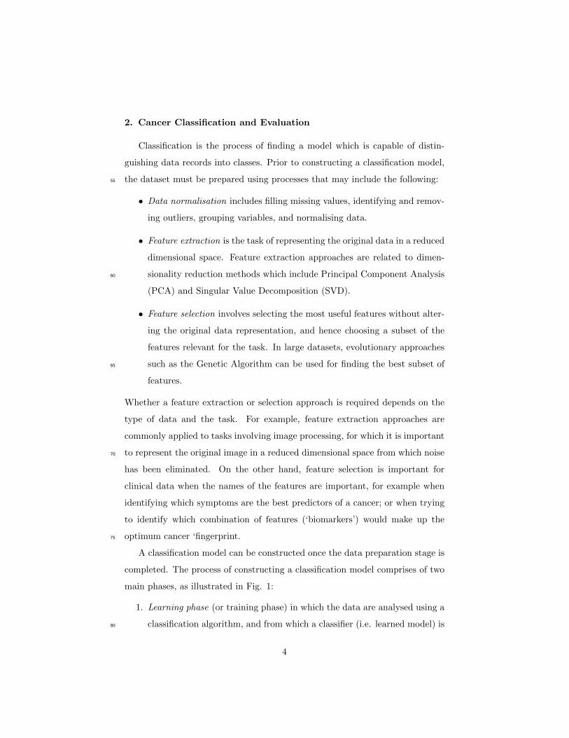
The Area Under the Curve is a reflection of how good the system’s perfor-
mance is at discriminating between patients with and without disease, and the
larger the Area Under the Curve the better the performance. Examples of ROC
curves are presented in Fig. 2, which shows the results from evaluating the
efficacy of four different types of tumour markers, as prostate cancer predictors,185
at various cutoff points (Chadha et al., 2014).
8
Figure 2: Receiver operating characteristic (ROC) graphical representation of the relationship
between sensitivity and specificity. Each graph models the probability of local disease versus
metastatic prostate cancer. Each ROC curve evaluates the efficacy of a tumour marker, as a
prostate cancer predictor, at various cutoff points, and shows the Area Under the ROC curve.
The figure shows that PSA (Prostate-Specific Antigen) and TNF (tumor necrosis factor-α)
levels were the strongest predictors of local versus metastatic disease. Soluble tumor necrosis
factor-α receptor 1 (sTFNR1) was also a reasonably good predictor (Chadha et al., 2014).
9

3. Computational Intelligence Approaches to Prostate Cancer Pre-
dictive Modeling
Computational intelligence concerns the theory, design, application, and de-
velopment of biologically and linguistically motivated computational paradigms190
which include Artificial Neural Networks, Genetic Algorithms, Evolutionary al-
gorithms, Fuzzy systems, and hybrid intelligent systems. In contrast, compu-
tational intelligence is efficient in solving problems which require reasoning and
decision-making and which traditional statistical models often fail to handle,
mainly due to uncertainty, noise and dynamically changing data. This section195
describes the literature on computational intelligence approaches that have been
applied to the prognosis and diagnosis of prostate cancer.
3.1. Artificial Neural Networks
Artificial Neural Networks are learning algorithms that are inspired by bi-
ological neural networks (the central nervous systems of the brain), and they200
consist of a set of interconnected input/output units in which each connection
has an associated weight. The interconnected ‘neurons’ send messages to each
other and their numeric weights can be tuned on the basis of the neural network’s
experience, thereby making neural networks adaptive to inputs and capable of
learning. During the learning phase, neural networks learn by adjusting their205
weights in order to predict the class label of the input records. Neural networks
must be trained for long periods of time before they can be applied to solving
problems such as classification or prediction. The limitation of the Artificial
Neural Network is that it is difficult for humans to understand the symbolic
meaning behind the learned weights of the hidden units in the network, which210
makes it difficult to understand the qualitative reasoning behind the decisions
that are made by the neural network. In addition, neural networks are more
prone to overfitting than other computational intelligence algorithms and hence
it is important to adopt a validation methodology, such as k-fold cross valida-
tion when reporting the performance of the neural network. The advantage of215
10
the Artificial Neural Network is that it often performs well with classifying data
which have not been included in the learning process (hence data that have
previously been unseen by the model).
3.1.1. Artificial Neural Networks on Clinical Data
Artificial Neural Networks have been applied to the early detection (Stephan220
et al., 2009) and diagnosis of prostate cancer (Djavan et al., 2002), and for the
prediction of its outcome (Ecke et al., 2012). Neural networks are also effective
for early diagnosis of prostate cancer when integrated into expert systems. The
performance of the Artificial Neural Network has been compared to that of
nomograms for detecting prostate cancer, and the vast majority of the literature225
supports the proposition that Artificial Neural Networks perform better than
nomograms for risk prediction, and disease diagnosis and prognosis (Shariat
et al., 2009a).
Interestingly, some studies have found that the predictive performance of
the nomograms was close to that of the Artificial Neural Network, and that the230
performance of these models is dependent on the data and task in question.
However, the outcomes of such studies were inconclusive. For example, Ecke
et al. (2012) compared the performance of Artificial Neural Network against the
nomograms developed by Karakiewicz et al. (2005) and Kawakami et al. (2008),
and found that, during the testing phase, each of the methods performed very235
similar to each other, with no definitive answer to which is best. Consequently,
they concluded that Artificial Neural Networks would be more successful for
increasing detection rates, in daily practice, than nomograms. Artificial Neu-
ral Network classifiers have been applied for early diagnosis of prostate cancer
and aiding the decision-making process without the need to perform a biopsy240
on patients. Cinar et al. (2009) applied an Artificial Neural Network and Sup-
port Vector Machines for early prostate cancer diagnosis on a reduced dataset
(which comprised features: Prostate Specific Antigen (PSA), prostate volume,
density, and smoking). To obtain the set of reduced features, they applied in-
dependent sample t-test statistical analysis as a technique for feature selection.245
11

The performance of the Artificial Neural Network was compared to that of the
Support Vector Machine classifier, and the results revealed that the Artificial
Neural Network and Support Vector Machine performances were very close.
The performance of the Artificial Neural Networks reached its highest with 81%
sensitivity, 77.9% specificity, and 79.1% accuracy, whereas the Support Vector250
Machine reached its highest performance with 84.2% sensitivity, 74.8% speci-
ficity, and 81.1% accuracy, thereby slightly outperforming the neural network.
Similarly, Saritas et al. (2010) devised an Artificial Neural Network for the
prognosis of cancer, the aim of which was to help doctors to decide whether
a biopsy is necessary. They used data obtained from 121 patients who were255
definitively diagnosed with cancer after biopsy. Their results revealed an Area
Under the Curve of 94.44%, thereby suggesting that an Artificial Neural Network
system can help doctors make quick and reliable diagnoses. However, these
results appear to be inconclusive due to the very small dataset which was used
and validation methodology adopted – 92 randomly selected records (n = 92,260
70% of the total data) were used for constructing the dataset used for training
the Artificial Neural Network, and the remaining 29 data records (n = 29, 30%
of the total data) were used for constructing the test dataset.
It is important to mention that when comparisons between prediction mod-
els, nomograms and other statistical models, are carried out, the same data265
and evaluation measures must be used for evaluating the predictive accuracy of
the models in order to allow a fair comparison between them. This will reveal
whether computational approaches are superior to nomograms when trained
and tested on small datasets. Such a comparison is described in Cosma et al.
(2016).270
3.1.2. Artificial Neural Networks on Images
Artificial Neural Networks have been applied to the detection of prostate
cancer using data obtained from transrectal ultrasonography and magnetic res-
onance images. In a study by Lee et al. (2006), the diagnostic performance of an
Artificial Neural Network model was evaluated in the presence and absence of275
12

transrectal ultrasonographic (TRUS) data which was obtained from 684 consec-
utive patients who had undergone TRUS-guided prostate biopsy. Their results
revealed that performance improved when TRUS findings were included, with
the ROC analysis revealing an average AUC of 85%.
Artificial Neural Networks have also been successfully applied to determine280
the probability of malignancy by classifying information extracted from multi-
parametric Magnetic Reasonance Imaging (MRI) (Vos et al., 2012). When the
performance of the Artificial Neural Network was compared to the systematic
biopsy, the results revealed that it can achieve a lower false positive rate than
systematic biopsy, and hence it can be utilised as a tool to assist radiologists285
and guide biopsies to the most aggressive location of the cancer. Using a similar
application of neural networks, Matulewicz et al. (2014) have assessed whether
an Artificial Neural Network can be utilised to detect cancer using information
extracted from endorectal magnetic resonance imaging and magnetic resonance
spectroscopic imaging (endo MRI/MRSI), and also information about anatomi-290
cal segmentation. The Artificial Neural Network achieved a high accuracy with
an Area Under the Curve, sensitivity and specificity of 96.8%, 62.5% and 99.0%
respectively. Although the dataset used for performing the evaluations was very
small and attributed to data availability, combining data obtained from images
with information about anatomical segmentation is a promising way forward for295
improving detection rates.
A hybrid Neural Network and Support Vector Machine system has been em-
bedded in a Computer-Aided Diagnosis (CAD) tool for predicting the Gleason
Grade of prostate cancer using histopathology images (Greenblatt et al., 2013).
This system uses the quaternion wavelet transform and modified local binary300
patterns for the analysis of image texture in regions of interest; and then utilises
a two-stage classification method for predicting the Gleason grade. Firstly, a
quaternion neural network with a new high-speed learning algorithm used for
multi-class classification is applied; aftre which several binary Support Vector
Machine (SVM) classifiers are used for classification refinement. Experimen-305
tal evaluations using the leave-one-out cross validation approach to predict the
13
Gleason grades (3, 4, and 5) using a dataset of 71 images revealed a high degree
of accuracy, 98.87%, and also that it outperformed other published automatic
Gleason grading systems. When results were averaged over all the classes, the
system achieved a specificity rate of 99% and a sensitivity rate of 96.7%. In310
the signal processing field, quaternions have been employed in adaptive filter-
ing, including Kalman filtering (Choukroun et al., 2006) and stochastic gradient
type of algorithm, such as the Quaternion Least Mean Square (QLMS) (Took
& Mandic, 2009).
3.1.3. Deep Learning Networks315
Deep Learning is a sub-field of machine learning composed of models com-
prising multiple processing layers to learn representations of data with multiple
levels of abstraction (Guo et al., 2016). Deep Learning models comprise mul-
tiple levels of distributed representations, with higher levels representing more
abstract concepts (Bengio, 2013). Deep Learning algorithms are known for320
their capability to learn features more accurately than other machine learning
algorithms, and are considered to be promising approaches for solving data an-
alytics tasks with high degrees of accuracy. Recently, the Deep Neural Network,
which is a variation of the standard Artificial Neural Network, has received
attention. Many types of Deep Neural Networks exist, some of which are the325
Deep Boltzmann Machines (Salakhutdinov & Hinton, 2009), the Restricted Deep
Boltzmann machine (Hinton & Sejnowski, 1986), and the Convolutional Deep
Belief Network (Lee et al., 2009). These methods have dramatically improved
state-of-the-art natural language processing (Mikolov et al., 2013), computer
vision (Ciresan et al., 2012), as well as many other applications such as drug330
discovery and genomics (LeCun et al., 2015), and the analysis carcinoma images
(Arevalo et al., 2015a). Convolutional neural networks have been applied for
classifying mass lesions following mammography (Arevalo et al., 2015b). The
Deep Boltzmann Machine has been applied for feature representation and fu-
sion of multi-modal information from Magnetic Resonance Imaging (MRI) and335
Positron Emission Tomography (PET) for the diagnosis Alzheimer’s Disease
14

(AD) and Mild Cognitive Impairment (MCI) (Suk et al., 2014). The authors
applied the system to solve three binary classification problems of AD versus
healthy Normal Control (NC), MCI versus NC, and MCI converter versus MCI
non-converter. Their results revealed that the system was highly accurate, with340
maximal accuracies of 95.35%, 85.67%, and 74.58%, respectively, thereby out-
performing the competing methods. The authors concluded that the proposed
Deep Learning method could hierarchically discover the complex latent patterns
that are inherent in both MRI and PET. These findings highlight the potential
value of Deep Learning on multi-modal neuro-imaging data for aiding clinical345
diagnosis. The application of Deep Learning algorithms to prostate cancer is
starting to emerge. Guo et al. (2015) proposed a deep-learning based approach
for the segmentation of the prostate using Magnetic Resonance (MR). Instead
of training a classifier using handcrafted features, the authors have proposed a
Deep Neural Network based approach which learns the feature hierarchy from350
the data. They found that the learned features were often more accurate in
describing the underlying data than the handcrafted features.
Deep Belief networks are another type of Deep Learning Networks. Deep
Belief networks are probabilistic generative models that are composed of multi-
ple layers of stochastic, latent variables. Azizi et al. (2015) have developed an355
automatic feature selection framework for analysing temporal ultrasound signals
of prostate tissue. The framework is based on a Deep Belief Network (DBN)
model and consists of: an unsupervised feature reduction step that applies the
model on spectral components of the temporal ultrasound data; and a super-
vised fine-tuning algorithm that uses the histopathology of the tissue samples to360
further optimize the model. Finally, a Support Vector Machine (SVM) classifier
uses the activation of the Deep Belief Network as input to predict the likelihood
of cancer.
3.2. Fuzzy Approaches
Traditional classification algorithms such as the Artificial Neural Network365
and the Support Vector Machine group each item into a single set (or class). In
15
classical set theory, sets can wholly include or wholly exclude any given element
(i.e. item). A fuzzy set is a set without a crisp or clearly defined boundary
and can therefore contain elements with partial degrees of membership. Fuzzy
rule-based systems are mathematical models that are based on fuzzy set theory370
(Zadeh, 1965), and are suitable approaches for solving classification and pre-
diction problems in circumstances in which an item can partially belong to one
or more sets (assigned a degree of membership for each set). Such approaches
therefore resemble human-like reasoning. Fuzzy rule-based systems have been
especially designed for dealing with the uncertainty and the imprecision found in375
data which are typical in medical data that are used for prognosis and diagnosis
of disease in patients.
As an example, one could consider the task of predicting the prostate cancer
stage of patients so that the prediction can assist clinicians when deciding on the
best treatment for the patient. Assume that true is represented by the numerical380
value of 1 and false the numerical value of 0, fuzzy logic permits in-between
values like 0.35 stage I and 0.74 stage II cancer. Hence, the values represent the
degree of membership of an element in set Stage I and set Stage II respectively.
This degree is computed via a membership function. A membership function
defines how each point in the input space is mapped to a membership value385
(or degree of membership) between 0 and 1. Fig. 3 illustrates a membership
function developed by Castanho et al. (2013) neuro-fuzzy system.
Fuzzy rule-based systems are suitable approaches for tasks which require
reasoning with data which contains degrees of uncertainty, as these approaches
provide a simple, IF-THEN rule-based approach to solve a problem. Fuzzy390
rules can be expressed using linguistic features (e.g. clinical test names, for
example: PSA, age) to create the rules which map inputs (e.g. clinical test
results: PSA=14.0, Gleason 1=4, Gleason 2=4, age=70, etc.) into outputs
(e.g. prostate cancer risk=Very High). Importantly, the derived rules (qual-
itative information) can be easily interpreted by clinicians. Fuzzy rule-based395
approaches add extra value to the prediction since they provide the reasoning
behind the prediction in the form of rules. For example, they could provide
16

Figure 3: Membership functions which refer to input variables of PSA level, Gleason score,
and Clinical stage (Castanho et al., 2013)
insight into which combinations of socio-demographic and early clinical features
increase a patient’s risk (useful for making predictions, and treatment decisions
personalised to patients).400
3.2.1. Neuro-Fuzzy Approaches
To date, fuzzy rule-based approaches are amongst the most popular ap-
proaches that have been applied to prostate cancer. Benecchi (2006) predicted
the presence of prostate cancer using a co-active neuro-fuzzy inference system
(CANFIS). CANFIS initially adopts a Genetic Algorithm (GA) to simultane-405
ously search for features and thereafter uses the selected features to derive the
fuzzy rules for prediction. Experiments were carried out with data from 1030
men, of which 195 (18.9%) had prostate cancer. All men had total prostate-
specific antigen (tPSA) level of less than 20 ng/mL. Men with a Prostate Specific
Antigen (PSA) level higher than 20 ng/mL in their bloodstream are likely (but410
not definitely) to have prostate cancer. The challenge in prostate cancer detec-
tion is to identify those men with prostate cancer who have PSA levels less than
20 ng/mL. A PSA level higher than 20 ng/mL may occur due to factors other
than cancer, such as urinary infection or an enlarged prostate. Their results
revealed that the predictive accuracy of CANFIS was superior to that of the415
PSA blood test. Similarly, Keles et al. (2007) have created a Neuro-Fuzzy Clas-
17

sification (NEFCLASS) tool for the diagnosis of prostate cancer, and prostate
enlargement diseases. The symptoms of prostate cancer are very similar to
those of prostate enlargement, and the aim of the classifier was to differentiate
between these two scenarios and hence assign them to different classes. The420
authors only used data from 90 cases (and 47 values were missing from these
cases), and concluded that the parameters of the NEFCLASS must be tuned for
better prediction performance. However, results were inconclusive due to the
small amount of data that were used to train and test the model.
Recently, Cosma et al. (2016) developed a neuro-fuzzy computational in-425
telligence model for classifying and predicting the likelihood of a patient hav-
ing Organ-Confined Disease (OCD) or Extra-Prostatic Disease (ED) using a
prostate cancer patient dataset obtained from The Cancer Genome Atlas (TCGA)
Research Network. The process for estimating the likelihood that the cancer
has spread before treatment is given to the patient, is known as cancer staging430
prediction. Such a prediction is important for determining the most suitable
treatment and optimal management strategy for patients. Clinical test results
such as the pre-treatment Prostate-Specific Antigen (PSA) level, the most com-
mon tumor pattern in tumour tissue biopsies (Primary Gleason pattern) and the
second most common tumor pattern (Secondary Gleason pattern), and the clin-435
ical T stage are commonly used by clinicians to predict the pathological stage of
prostate cancer. The neuro-fuzzy system by Cosma et al. (2016) takes as input
the results of those tests and an additional input, which is the age at diagno-
sis. Experiments revealed that the proposed neuro-fuzzy system outperformed
other computational intelligence based approaches, namely the Artificial Neural440
Network, Fuzzy C-Means, Support Vector Machine, the Naive Bayes classifiers.
The proposed neuro-fuzzy system also performed better than the AJCC pTNM
Staging Nomogram (Edge et al., 2010) which is commonly used by clinicians.
At its optimal point, the neuro-fuzzy system returned the largest Area Un-
der the ROC Curve (AUC), with a low number of false positives (FPR = 0.274,445
TPR=0.789, AUC=0.812). The proposed approach is also an improvement over
the AJCC pTNM Staging Nomogram (FPR=0.032, TPR=0.197, AUC=0.582).
18

3.2.2. Genetic-Fuzzy Approaches
Using a different application of the fuzzy rule-based approach, Castanho
et al. (2013) have developed a Genetic-Fuzzy expert system to predict the patho-450
logical stage of prostate cancer. Such a prediction impacts on the treatment
decision provided to patients. Their proposed Genetic-Fuzzy system tunes the
fuzzy rules and membership functions using a Genetic Algorithm. Their system
achieved an Area Under the Curve of 82.4% which was compared against a sys-
tem which uses Partin probability tables (i.e. nomogram) that only achieved455
and Area Under the Curve of 69.3%. It should be noted that in the study by
Castanho et al. (2013), the Genetic Algorithm was used for membership func-
tion tuning, whereas in previous studies such as that by Benecchi (2006), the
Genetic Algorithm was used for feature extraction. This demonstrates the suit-
ability of the Genetic Algorithm for tuning membership functions and feature460
extraction tasks.
3.2.3. Evolutionary Fuzzy Cognitive Maps
A Fuzzy Cognitive Map (Kosko, 1986) is an extension of cognitive maps
which inherited the main aspects of fuzzy logic and Artificial Neural Networks
for graphically representing the reasoning behind a given domain of interest.465
Fuzzy Cognitive Maps describe a system using nodes/concepts (variables, states)
and signed fuzzy relationships between them. Although the Fuzzy Cognitive
Map bears a resemblance to an Artificial Neural Network, it is a conceptual
network and therefore the nodes and arcs within the Fuzzy Cognitive Map are
able to follow semantical interpretation. The advantage of Fuzzy Cognitive470
Maps over Artificial Neural Networks is that knowledge about the casual de-
pendencies within the domain of interest is transparent and hence it can be
easily interpreted by humans. However, a limitation of Fuzzy Cognitive Maps
is that they are constructed manually, and therefore it may not be feasible to
apply them when dealing with data comprising of a large number of variables.475
In order to address this limitation, Froelich et al. (2012) proposed an evolution-
ary Fuzzy Cognitive Map approach which is capable of learning Fuzzy Cognitive
19

Maps. The proposed evolutionary Fuzzy Cognitive Map was applied to predict
a patient’s state after a period of time following a suggested therapy plan. The
evolutionary Fuzzy Cognitive Map was applied to a small dataset comprising of480
40 patients suffering with prostate cancer. The results revealed that the evo-
lutionary Fuzzy Cognitive Map outperformed the basic Fuzzy Cognitive Map.
Although it is difficult to determine the reliability of the results given the small
dataset, it is important to appreciate that the authors gave appropriate thought
to the validation of the results in order to ensure reliability of findings. They ap-485
plied two methods to validation - method 1: the data were divided into learning
and testing sets of the same cardinality (the learning set contained records of 20
patients, the remaining 20 records constituted the testing set); and method 2:
the leave-one-out cross validation (LOOCV) method was applied. The results
revealed that both validation methods returned very similar results, and this490
may not have been the case if a larger dataset was utilised.
3.3. Support Vector Machines
Support Vector Machine (SVM) (Cortes & Vapnik, 1995) is a method for
the classification of linear and nonlinear data, and uses nonlinear mapping to
transform the original training data into a higher dimension. Support Vector495
Machines then search for the linear optimal separating hyperplane, which es-
sentially is a boundary which separates the records into classes. The Support
Vector Machine finds the optimal hyperplane using support vectors (which can
be characterised as the most significant training records) and margins (which
are defined by the support vectors) (Han et al., 2011). The Support Vector500
Machine can be trained using several functions: the Linear Kernel Function,
Quadratic, Gaussian Radial Basis (GRB), Multilayer Perceptron Kernel (MP)
functions. Fig. 4 shows an example Support Vector Machine applied to ovarian
cancer prediction using a linear separation of classes (Gaul et al., 2015). The
most suitable training function is often experimentally selected. Support Vector505
Machines, when trained using the appropriate training function, are highly accu-
rate and capable of modeling complex nonlinear decision boundaries (Han et al.,
20

Figure 4: (a) Accuracy using Support Vector Machine (SVM) feature selection for metabolic
detection of early stage ovarian cancer. Plot (a) shows the performance of the SVM based
classifier against alternative approaches. A minimum of 16 metabolic features that provided
100% accuracy. Plot (b) shows the optimal linear separation between epithelial ovarian cancer
(EOC) and control samples by the SVM-based model. The vertical line is the projection of
the separating hyperplane generated by the SVM model. The discriminant linear SVM model
was evaluated by leave-one-out cross-validation (LOOCV) (Gaul et al., 2015).
2011). They are also much less prone to overfitting than other computational
intelligence methods, and can be used for classification as well as prediction
tasks. Support Vector Machines have been adopted to solve decision-making510
tasks on data which also include data obtained from images, microarray and
other clinical data.
The automatic identification of the boundary between the prostate and non-
prostate regions is challenging, as the low contrast of ultrasound prostate images
makes prostate and non-prostate boundaries fuzzy and noisy. Computational515
intelligence methods can be applied to identify and segment the prostate region
on ultrasound images. Sung et al. (2011) proposed a Computer-Aided Diagnosis
(CAD) system, based on Support Vector Machines, for prostate cancer detec-
tion using dynamic contrast-enhanced MRI (DCE-MRI) examinations. Their
system was evaluated using DCE-MRI examinations of 42 patients, and the520
results revealed that the system achieved an overall accuracy, sensitivity and
21

specificity of 83%, 77% and 77% respectively. In a recent study, Haq et al.
(2015) also produced a DCE-MRI system for prostate cancer prediction. The
approach by Haq et al. (2015) is data-driven and utilises a number of approaches
for feature extraction and feature reduction. In particular, Principal Compo-525
nent Analysis (PCA) was applied along with the least absolute shrinkage and
selection operator (LASSO) to extract the optimal set of principal components.
Using the extracted features, a predictive model was created which was based
on the Support Vector Machine classification algorithm. For testing the model,
a total of 449 tissue regions were obtained from 16 patients, and the results530
revealed that the proposed system achieved an Area Under the Curve of 86%
when using the leave-one-out cross validation approach.
Fei et al. (2011) have developed a PET/CT directed, 3D ultrasound image-
guided biopsy system for improving the detection of prostate cancer. Their
system was designed to automatically identify the areas of an image containing535
prostate and non-prostate tissues. The prostate textures were captured by train-
ing the locally placed Wavelet-based Support Vector Machines (W-SVMs). The
trained W-SVMs were used to tentatively label the voxels around the surface
into prostate and non-prostate tissues based on their texture features obtained
from different Wavelet filters. Thereafter, boundaries were formed between the540
tentatively labelled prostate and non-prostate tissues based on defined weighting
functions and labeled voxels. The authors found that, using local texture fea-
tures and geometrical data, W-SVMs can improve the classifier’s performance
with regards to differentiating the prostate tissue from the adjacent tissues.
They also found that TRUS image textures can provide important features545
for accurately defining the prostate, particularly for the regions where prostate
boundaries are not clear. The system was evaluated using data sets contain-
ing 3-D TRUS images from 5 patients. The system achieved an average DICE
overlap ratio of 90.7%± 2.5%, and an average sensitivity of 90.7%± 4.9%.
Fig. 5 shows sample segmentation and its comparison with the corresponding550
gold standard (obtained from manual segmentation) (Fei et al., 2011). Briefly,
the DICE overlap ratio is the result of using the DICE coefficient (Dice, 1945)
22

Figure 5: 2-D segmentation results in different planes: red lines are the gold standard bound-
aries (those defined by experts) and green lines are the segmentation boundaries (those defined
by the system which uses Wavelet-based Support Vector Machines, W-SVMs). (a)Coronal
plane (b) Sagital plave (c) Transverse plane (Fei et al., 2011)
which measures the extent of spatial overlap between two binary images. It
is commonly used in reporting performance of segmentation and gives more
weighting to instances where the two images agree. A DICE overlap ratio value555
ranges from 0 (or 0%), indicating no spatial overlap between two sets of binary
segmentation results, to 1 (or 100%), indicating complete overlap and there-
fore perfect agreement. The performance of the system proposed by Fei et al.
(2011) was tested on a very small dataset of images, and more evaluations need
to be conducted to conclude on the systems overall accuracy in automatically560
identifying the areas of an image containing prostate and non-prostate tissues.
Similarly, Kim & Seo (2013) proposed an approach for segmenting prostate
tissues using TRUS images and Gabor texture features, snake-like contour
smoothing algorithm and the Support Vector Machine algorithm. Gabor fea-
ture extraction was applied to smooth the image and remove speckle noises, and565
the snake-like contour algorithm was then implemented to conclusively define
the boundary of the prostate. After identifying the pixels defining the prostate
boundary, the Support Vector Machine was trained using the pixels and known
class labels (as identified by human experts) for classifying the pixels within
prostate and non-prostate. During the testing phase, the accuracy of the algo-570
rithm in identifying the pixels defining the outline for the prostate boundary is
compared to the results of a human expert who performed the same task. A
23
total of 20 experimental images were used for the tests and the results revealed
that the prostate boundaries generated differed from those that were drawn by
human experts by only 10%. More recently, a system proposed by Lehaire et al.575
(2014) used Support Vector Machines in combination with feature extraction for
distinguishing between normal, normal but suspicious, and aggressive classes of
cancer tissue found in multi-parametric magnetic resonance (mp-MR) images.
The system was evaluated using mp-MR images of 35 patients. The system
achieved a mean Area Under the Curve of 78%± 1%, which compares well with580
other current state of the art systems.
Gertych et al. (2015) emphasise that although image classification approaches
have been developed to identify and classify glandular regions in digital images
of prostate tissues, the success of these has been limited by their capability to
identify the different types of tissue components such as stroma, benign/normal585
epithelium and prostate cancer. They proposed a machine learning approach
comprising of a Support Vector Machine followed by a Random Forest classi-
fier to differentiate prostate tissue into stroma, benign/normal epithelium and
prostate cancer areas. A total of 210 high resolution images of low-grade and
high-grade tumors which were collected from 20 radical prostatectomies were590
manually annotated by two pathologists. The 210 images were split into the
training (n = 19) and test (n = 191) sets. In the pre-processing steps, the
Support Vector Machine separated the areas of stroma from the epithelium.
Subsequently, areas of epithelium were stratified into benign/normal glands and
prostate cancer using the Random Forest classifier. The Random Forest classi-595
fier was trained with a different number of trees. Algorithms were evaluated by
Jaccard (J), area overlap (O) and Rand indices (Ri) in order to determine the
concordance of the algorithm-based prediction with pathologist manual anno-
tations. J and O indices for concordance of stroma and epithelium areas were
calculated separately, whereas Ri was calculated for stroma and epithelium to-600
gether. To distinguish benign/normal glands from prostate cancer they trained
a Random Forest classifier and obtained separate performance values for be-
nign/normal glands and prostate cancer: JBN = 35.2± 24.9, OBN = 49.6± 32,
24
JPCa=49.5± 18.5, OPCa=72.7± 14.8 and Ri = 60.6± 7.6.
Singireddy et al. (2015) devised a Support Vector Machine classifier to iden-605
tify biomarkers associated with prostate cancer progression (i.e. cancer stage)
using RNA-Seq and the Support Vector Machine classifier. They utilised the
Minimum Redundancy Maximum Relevance (mRMR) (Peng et al., 2005) statis-
tical approach to select the best features, and thereafter a linear Support Vector
Machine for performing the classification task. Although the reported accuracy610
was high, in the range of 80% to 99.3%, this was a small-scale study which used
a dataset of 106 prostate cancer samples. The authors do not report on the
validation approach, nor whether the results reported were of the training or
testing stage. Luque-Baena et al. (2014) performed a comparative study of the
Stepwise Forward Selection (SFS) and Genetic Algorithms for the analysis of615
microarray data, with the aim of identifying groups of genes which have high
predictive capability and biological relevance. They found that the predictive
models returned higher accuracies when the Genetic Algorithm was utilised to
select features as opposed to the Stepwise Forward Selection approach.
In summary, the automatic identification of the boundary between prostate620
and non-prostate continues to be challenging given that the boundary is often
not clear in ultrasound prostate images and that their textures are difficult to
classify. The identification and classification of cancerous and non-cancerous tis-
sues by analysing image data is also a challenging and ongoing area of research.
A common barrier relates to the availability of datasets which are large enough625
to ensure that the reported system performance is indeed representative. How-
ever, the studies conducted thus far in this area are yielding promising results.
With regards to extracting relevant features from microarray data, this is also
a very complex task because this type of data comprises a large number of fea-
tures while few samples are generally available (Luque-Baena et al., 2014). The630
use of metaheuristic optimisation approaches for feature selection and bound-
ary identification warrant examination, and the applications of metaheuristic
optimisation algorithms to prostate cancer are discussed in Section 3.4.
25

3.4. Metaheuristic Optimisation
Metaheuristic optimisation algorithms are designed to solve complex optimi-635
sation problems and are applied to find, generate, or select a heuristic (partial
search algorithm) that may provide a sufficiently good solution to a problem.
Metaheuristic algorithms are especially effective when the information is uncer-
tain and dynamic (Bianchi et al., 2009). Some of the most popular metaheuris-
tics include the Genetic Algorithm (Holland, 1992), Particle Swarm Optimisa-640
tion (Kennedy & Eberhart, 1995), Artificial Bee Colony algorithm (Teodorovic
et al., 2006), and Ant Colony optimisation algorithm (ACO) (Dorigo & Gam-
bardella, 1997). Many of these nature-inspired algorithms are developed by
studying the evolutionary behaviour of species (e.g. birds, insects, humans) and
mimicking this in a computer science algorithm. Metaheuristic optimisation ap-645
proaches are most commonly used for finding the best features in large datasets.
These approaches require their parameters to be carefully tuned using suitable
parameter values which need to be adapted based on the dataset and problem to
be solved. Furthermore, models which comprise of a collection of optimisation
and classification algorithms can be easily over-trained and extensive evalua-650
tions using appropriate validation approaches must therefore be carried out. In
the subsections that follow, the metaheuristic optimisation approaches which
have been applied to derive prostate cancer predictive models are discussed.
3.4.1. Genetic Algorithm
A Genetic Algorithm is an evolutionary algorithm (also known as a search655
heuristic or metaheuristic) which generates solutions to optimisation and search
problems. Genetic Algorithms use techniques inspired by natural evolution, such
as inheritance, mutation, selection, and crossover, and are often combined with
other computational intelligence approaches to solve classification and predic-
tion problems. Underwood et al. (2012) developed a Genetic Algorithm based660
method that integrates a simulation model in a Genetic Algorithm with the aim
of selecting the best Prostate Specific Antigen (PSA) test screening policy. Com-
parisons between the results obtained from their proposed method and previ-
26
ously recommended screening policies revealed that patients should be screened
more aggressively, but for a shorter length of time than previously published665
guidelines recommend. Their research clearly demonstrates how computational
intelligence can be used to influence healthcare policies. Treatment planning
for radiation therapy is a multi-objective optimisation process. Yu et al. (2000)
present a machine intelligent scheme for the planning of radiation therapy which
is based on Multi-Objective Decision Analysis (MODA) and Genetic Algorithm670
(GA) optimisation. They found that a combination of MODA and GA optimi-
sation can provide solutions to practical treatment planning tasks. The authors
emphasise the potential for real time applications in radiotherapy. Shi et al.
(2013) propose a new approach to segment prostate ultrasound images using the
Genetic Algorithm optimisation. Boundary curve representations are derived675
by using Principal Component Analysis (PCA), after which prostate boundary
features are determined and a Genetic Algorithm applied in order to optimize
the parameters of the implicit curve representation. Recently, McGeachy et al.
(2015) developed a Simple Genetic Algorithm (SGA) for determining optimal
seed distributions for low-dose-rate prostate brachytherapy (McGeachy et al.,680
2015). The SGA performance was evaluated by comparing solutions obtained
from a commercial optimizer (Inverse Planning Simulated Annealing [IPSA])
with the same cohort of 45 patients. The results of the SCGA and the IPSA
were similar, and clinically acceptable. The Genetic Algorithm has also been
used in various hybrid models in which it has been used to optimise the perfor-685
mance of a classifier, or for feature selection tasks. For example, Castanho et al.
(2013) proposed a hybrid rule-based fuzzy system for predicting the pathologi-
cal stage of prostate cancer, which uses a Genetic Algorithm to tune the fuzzy
rules and membership functions was discussed in Section 3.2.2. Other hybrid
algorithms which use Genetic Algorithms are discussed in the relevant sections690
of the paper.
27
3.4.2. Ant Colony Optimisation
In computer science, the Ant Colony optimisation algorithm (ACO) (Dorigo
& Gambardella, 1997) is a probabilistic technique for solving computational
problems that are concerned with finding the best paths through graphs. Ant695
Colony optimisation algorithms are based on the behaviour of ants seeking a
path between their colony and a source of food - ants search for, and mark, the
best solutions and take account of previous markings to optimize their search.
Ant Colony optimisation has been applied to solve a variety of issues, including
classification (Martens et al., 2007) and data mining problems (Parpinelli et al.,700
2002). In the prostate cancer classification system proposed by Thangavel &
Manavalan (2014), Ant Colony Optimisation was applied to select the best fea-
tures for detecting prostate cancer from TRUS images. Initially, the Regions
of Interest (RoI) were identified from the TRUS images and thereafter optimi-
sation approaches were applied to the selected Regions of Interest in order to705
find the best features. Rough set based algorithms (namely the Hybridization
of rough set based Quick Reduct) were combined with the Ant Colony Opti-
misation (QR-ACO) algorithm for selecting the best features from the selected
Regions of Interest of TRUS images in order to improve accuracy and efficiency
(feature selection). As an alternative to QR-ACO, a Genetic Algorithm-Ant710
Colony Optimisation (GA-ACO) algorithm was also developed for reducing the
feature set. Once the best features were selected, the Support Vector Machine
was applied for classifying the images to benign and cancer. Their experimental
results revealed that the Ant Colony optimisation algorithm is an efficient ap-
proach for selecting the minimal features that are required for highly accurate715
classification of cancer and benign images.
3.4.3. Particle Swarm Optimisation
The Particle Swarm Optimisation (PSO) approach (Kennedy & Eberhart,
1995) is an adaptive, randomly optimal algorithm which is constructed on swarm
intelligence, as each particle within the swarm represents a possible solution to720
the optimisation problem. In a Particle Swarm Optimisation system, a particle
28
is within the search space and, with each iteration, it adjusts its position on the
basis of its own experience and that of nearby particles. The particles evaluate
their own position on the basis of a fitness function, and the process is repeated
until the number of iterations have been exceeded. Sadoughi & Ghaderzadeh725
(2013) have developed a system to support the diagnosis of prostate cancer which
combines the features of a Back Propagation Neural Network (BPNN) with
particle swarm optimisation host. The authors used a dataset from 360 patients
who underwent radical prostatectomy for prostate cancer. The dataset is a two-
class problem, either positive or negative, for cancer and benign hyperplasia730
of prostate (BPH) diseases respectively. Sensitivity, specificity, and accuracy
were recorded for the system during training and achieved 96.87%, 100% and
98.33%, respectively. The authors note that while the system does not produce
a concrete diagnosis for prostate cancer, it does provide information for doctors
to help assess whether a biopsy is necessary.735
3.4.4. Artificial Immune System
The Artificial Immune System (AIS), first proposed by Jerne (1974) are
another type of metaheuristic learning algorithm which has been designed to
solve optimisation problems. AIS algorithms are inspired by the principles of
theoretical immunology and the processes of the vertebrate immune system740
(Tang & Vemuri, 2005). The vertebrate immune system has many specialized
cells and molecules that interact in particular ways. AIS algorithms typically
exploit the immune system’s characteristics of learning and memory to solve a
problem.
Kuo et al. (2015) have developed a model based on the AIS for the prognosis745
of prostate cancer which also uses a two-stage fuzzy neural network. Regression
analysis was initially performed to find out the important factors which affect
prognosis, and these factors included age, Body Mass Index (BMI), Prostate
Specific Antigen (PSA), Digital Rectal Examination (DRE), clinical T-stage,
biopsy, and treatment methods. These important factors are then applied to a750
fuzzy neural network. The fuzzy neural network comprised two steps. During
29

the first stage, clustering of the features was performed using the aiNET-K
clustering algorithm which is based on an Artificial Immune Network (Kuo
et al., 2014) in order to find a good initial solution for the membership functions
at the beginning of training. During the second stage, the Artificial Immune755
Network was integrated with Particle Swarm optimisation (called Opt-aiNET)
for the training of a fuzzy neural network. Through iterative evolution, the
algorithm tries to find the optimal solutions. The system was trained using a
small dataset comprising of 100 records and using 10-fold cross validation. Their
experiments revealed that the proposed method has the potential to accurately760
predict prostate cancer, and that it outperformed the network-based fuzzy logic
control system. The drawbacks of the proposed algorithm are computational
time and parameter tuning.
3.5. Ensemble Learning Approaches
Ensemble learning is the process by which multiple models, such as classi-765
fiers, are strategically generated and combined to solve a particular problem.
Ensemble learning algorithms are mainly used for classification and prediction
problems and are considered to be effective in achieving high performance.
An Ensemble method combines a number of k learned base classifier models,
M1,M2, . . . ,Mk, and aims to create an improved classification model, M∗, which770
is a combination of all the classifiers. A dataset, A, is decomposed into a to-
tal of k training sets, such that A1, A2, . . . , Ak, where all, but one datasets,
Ai(1 ≤ i ≤ k − 1), are used to train each classifier Mi. The remaining dataset
is used for validating the predictive accuracy of each classifier, and hence the
records found in this dataset have not been previously seen by any of the classi-775
fication models. During the classification process, a record Xi is passed to each
classification model which then returns a vote (i.e. class label) for the given
record. The Ensemble algorithm then returns a final class prediction which is
based on the majority of the votes of the base classifiers (Han et al., 2011).
Alternative Ensemble methods such as bagging, boosting and Random Forests780
have been created for deriving the final prediction (i.e. processing of multiple
30
votes to reach a final prediction). The Ensemble approach described above is
illustrated in Fig. 6.
Ensemble models reflect the real life decision making process where several
opinions may be gathered, and then all opinions are considered to make a final785
decision. For example, individual opinions of several experts are typically taken
into consideration before making a final decision and agreeing on a medical
procedure to minimise errors and optimise patient treatment (Polikar, 2009).
The purpose of adopting, and ensemble approach which comprises several
classifiers, as opposed to adopting a single classifier to solve a problem could be790
due to one or more of the following reasons (Polikar, 2009):
• Statistical reason: Ensemble algorithms are suitable when there is inade-
quate data to properly represent the data distribution;
• Computational reason: Ensemble models are chosen when there are many
computational models which are suitable to solving a given problem, and795
there is uncertainty as to which model to apply for solving the problem;
and
• Representational reason: certain problems are too difficult for a single/given
classifier to solve, meaning that the decision boundary that separates data
from different classes may be too complex for the classifier to learn. How-800
ever, an appropriate combination of an Ensemble of classifiers may be
capable of learning the boundary.
3.5.1. Random Forests
Random Forests (Breiman, 2001) are an Ensemble learning method that cre-
ates a number of decision trees using a random selection of attributes. Decision805
trees are a popular method for various machine learning tasks. Decision trees
can grow to be very deep in order to be capable of learning irregular patterns.
For this reason, they tend to over-fit their training datasets (and hence per-
form better during the training than during the prediction tasks) due to their
31

Figure 6: Ensemble classification: Combining an Ensemble of classifiers for making a predic-
tion. A dataset is decomposed into k datasets which are used to generate a set of classification
models, M1, . . . ,Mk. A new data record is passed to each classifier, each classifier returns a
vote (i.e. chosen class label). All votes are combined to return a final class prediction (i.e.
class label). Adapted from Han et al. (2011).
high variance. The Random Forests Ensemble learning method aims to reduce810
variance by averaging multiple deep decision trees that have been trained on
different parts of the same training set (Hastie et al., 2001), and hence it is less
prone to overfitting noise and it is less prone to chance correlation. During the
classification process, each tree votes for a class label of a given record, and the
class label with the majority of the votes is considered to be the predicted class815
label. Random Forests have been shown to boost the performance of the final
model and are known to be more robust to errors and outliers when compared
to other Ensemble learning methods such as the AdaBoost learning method (see
Section 3.5.2).
Random Forests have been applied to predict rectal toxicity following prostate820
cancer radiotherapy (Ospina et al., 2014); to classify prostate cancer samples us-
ing a proteomic data set generated mass spectrometry data (Tong et al., 2004);
and to identify biomarker panels in serum datasets for the detection and staging
of prostate cancer (Fan et al., 2011). A recent application of Random Forest has
been reported by Mohareri et al. (2014) who have designed a system for comput-825
ing the probability of prostate cancer. Their system is based on a combination of
features which were extracted from a novel multi-parametric quantitative ultra-
sound elastography technique. The performance of the system was validated on
32

a dataset containing data from 10 patients undergoing radical prostatectomy.
A Random Forest classification algorithm was applied to the combination of830
data extracted from the images in order to separate the cancerous regions from
the non-cancerous regions, and to compute a probability for prostate cancer.
During evaluations, the system achieved an Area Under the Curve of 82%± 1%
using the leave-one-out cross validation, thereby demonstrating that this type
of system has potential for clinical use.835
Another interesting application of Random Forests for the prediction of bio-
chemical recurrence following prostate surgery has been proposed by Golugula
et al. (2011). For this, multimodal data (imaging and non-imaging data) was
collected and a hybrid approach combining Supervised Regularized Canonical
Correlation Analysis (SRCCA) with a Random Forest classifier created. Their840
proposed approach was applied on a cohort of 19 patients, all of whom had
radical prostatectomy, 10 of whom experienced biochemical recurrence within
5 years of surgery and 9 of whom did not. Their proposed approach reached
a maximum classification accuracy of 93%. Importantly, the authors empha-
sise that “computational challenges have limited the ability to quantitatively845
integrate imaging and non-imaging data channels with different dimensionality
and scales”; few attempts have been made to mine such data for the purpose
of constructing classifiers; and that no studies were found to “quantitatively
combine histology (imaging) and proteomic (non-imaging) measurements for
making diagnostic and prognostic predictions”.850
Frantzi et al. (2014) provide a very interesting discussion on biomarker re-
search and how it is continuously expanding in the field of clinical proteomics.
They discuss the technical proteomic platforms that are available along the
different stages in biomarker discovery, and clinical applications relating to
bladder cancer biomarker research. They emphasise that mass spectrometric855
techniques could provide highly valuable tools for biomarker research, and that
advances could provide biomarkers that are clinically applicable for disease di-
agnosis and/or prognosis.
Much more research into combining non-image clinical data such as clini-
33
cal data obtained from patient examinations and blood tests (biomarker and860
proteomic data) with data obtained from images needs to be performed. Due
to the uncertainty and noise found in clinical data, it is useful and important
to take into consideration multimodal data (imaging and non-imaging data)
when making predictions which can affect decision-making. The challenge is
to select the best features from the different types of data, and to be able to865
find the best combinations for solving the prediction task. Advanced compu-
tational intelligence techniques such as Ensemble learning methods are suitable
for such challenging problems for which the classification problem is complex
and a number of classifier results need to be considered for reaching a predicted
outcome.870
3.5.2. Adaboost Ensemble Method
Adaboost or adaptive boosting is a popular Ensemble method boosting al-
gorithm which is used for improving the accuracy of the learning method. As
previously mentioned, Ensemble algorithms apply a variety of classifiers and
then weigh the output of each classifier to reach a conclusion. Adaboost assigns875
a weight to each classifier’s predicted output (or vote) based on the performance
of the classifier. A classifier’s performance is computed using the error rate -
the lower the error rate, the better the performance of the classifier.
Doyle et al. (2012) have designed a boosted Bayesian multiresolution (BBMR)
system, the aim of which is to identify regions of prostate cancer on digital880
biopsy slides. Initially, the proposed system decomposes the image down into
a multiple resolution levels pyramid image. A Bayesian classifier for identifying
the cancerous regions at lower resolution levels is then applied. These regions
are then examined in greater detail at higher resolution levels - this approach
allows for a quicker and more efficient analysis of large images which would885
require more computational time compared to running the algorithm directly
at full (highest) resolution. A total of 10 image features are chosen from each
resolution level through the use of an Adaboost Ensemble method. The system
was tested on a set of 100 images, gathered from 58 patients, and evaluations
34

revealed that it achieved at its lowest, intermediate, and highest levels an Area890
Under the Curve of 84%, 83%, and 76% respectively. The authors found that
their proposed boosted Bayesian multiresolution (BBMR) system outperformed
both and individual features (no Ensemble) approach, and a Random Forest
classifier Ensemble obtained by bagging multiple decision tree classifiers. Com-
puterised image analysis is a challenge due to the size of the digitised histology895
images which contain hundreds of millions of pixels. Importantly, the authors
found that different classes and types of image features become more relevant for
discriminating between prostate cancer and areas of benign disease at different
image resolutions. It was therefore important to extract features from different
image resolutions (Doyle et al., 2012), as this improves image processing speed900
and system accuracy.
3.6. Bayesian Approaches
Bayesian classification is a probabilistic model which addresses the classi-
fication problem by learning the distribution of instances given different class
values. This section describes the Naive Bayesian and the Bayesian Belief Net-905
work classifiers.
3.6.1. Naive Bayesian Classifier
Naive Bayesian classification is based on Bayesian theorem of posterior prob-
ability. Although it is designed for use when predictors within each class are
independent of one another, it is known to work well even when that indepen-910
dence assumption is not valid. The Naive Bayesian approach, classifies data
in two steps. The first step is the training (i.e. learning) step which uses the
training input records to estimate the parameters of a probability distribution,
assuming that predictors are conditionally independent. The second step is
the prediction step, in which the classifier predicts any unseen test records and915
computes the posterior probability of that sample belonging to each class. It
subsequently classifies the test records according to the largest posterior prob-
ability. Some of the functions that can be used for tuning the Naive Bayesian
35
classifier include the Gaussian Distribution (i.e. normal distribution) and Ker-
nel Density Estimation functions, and selecting which one to use depends on920
the dataset. Bayesian approaches have been applied to predict prostate can-
cer risk and risk of high-grade disease for men who undergo a prostate biopsy
(Thompson et al., 2006). Strobl et al. (2015) demonstrated that a Bayesian
approach integrated with Markov Chain Monte Carlo (MCMC) can improve
the predictive performance of the well-known Prostate Cancer Risk Calculator925
(PCPTRC) tool, and also found that using Random Forests can consistently
over-fit the training data. The Prostate Cancer Risk Calculator (PCPTRC)
(Thompson et al., 2006) is a risk assessment tool that assesses patient risk, in
consultation of their primary care physician.
Mazzetti et al. (2011) have used a Bayesian classifier for identifying malig-930
nant areas in Magnetic Resonance Images. In particular, they developed a Dy-
namic Contrast Enhanced Magnetic Resonance Imaging (DCE-MRI) Computer-
Aided Diagnosis (CAD) system to determine whether a given image area con-
tains malignant tissue. The system can be used to help locate prostate cancer
and guide biopsy to avoid unnecessary sampling. The system performs noise935
filtering and feature extraction. A Bayesian classifier is then applied to the
extracted data to estimate the probability of malignancy. The dataset used by
the authors was small and only included 10 patients with prostate cancer, and
the evaluation results show that the system achieved an Area Under the Curve
of 89.9%, a sensitivity of 82.4% and specificity of 82.1%.940
3.6.2. Bayesian Network
Bayesian networks are probabilistic graphical models which model the depen-
dencies among subsets of attributes (Lacave & Dez, 2003). Bayesian networks
are also known as belief networks, Bayesian Belief Networks and probabilis-
tic networks. A Bayesian network consists of an acyclic directed graph, whose945
nodes represent random variables, and whose links represent relations among
them, along with a probability distribution over its variables. The nodes can
also correspond to actual variables given in the data or correspond to “hidden
36
variables” which are believed to form a relationship. For example, in the case of
medical data, a hidden variable may indicate a syndrome, representing a num-950
ber of symptoms that could characterise a disease (Han et al., 2011). Bayesian
Belief Networks are different to naive Bayes classifiers, in that Bayesian Belief
Networks do not assume class conditional independence. Class conditional inde-
pendence is when the value of a particular feature is independent of the value of
any other feature, given the class variable. If the assumption of class conditional955
independence holds, then the Naive Bayes classifier is a more accurate approach
than the Naive Bayesian approach.
Fig. 7 shows a simple belief network for six variables: FamilyHistory, Lung-
Cancer, PositiveXRay, Smoker, Emphysema, and Dyspnea. All six variables are
Boolean, meaning that they have a yes/no answer. The arcs in Fig. 7 represent960
casual knowledge about lung cancer, for example, people with FamilyHistory
of lung cancer and who are smokers have a greater risk of lung cancer. The
PositiveXRay variable is independent of whether a person has a FamilyHistory
of lung cancer or is a Smoker. Since the outcome of PositiveXRay is known,
then the results of the FamilyHistory or Smoker variables do not provide any965
additional information regarding PositiveXRay (Han et al., 2011). A Bayesian
network provides a conditional probability table (CPT) for each variable. Fig.
7 shows the conditional probability table for the variable LungCancer, where
the conditional probability for each known value of LungCancer is provided for
each possible combination of the value of its parents, for example,970
P(LungCancer=yes|FamilyHistory=yes, Smoker=yes)=0.8
P(LungCancer=no|FamilyHistory=no, Smoker=no)=0.9.
Bayesian networks have been applied to the analysis of genomic data, and
mainly for investigating relationships between data and different types of data
obtained from multiple platforms in the context of prostate cancer. Xutao975
et al. (2007) created a Bayesian network approach which uses mass spectrometry
and microarray data for cross-platform analysis of cancer biomarkers. Using
their proposed Bayesian network model, they were able to identify fourteen
genes/proteins as reliable serum biomarkers, including prostate specific antigen
37

Figure 7: Simple Bayesian belief network. (a) A proposed causal model, represented by a
directed acyclic graph. (b) The conditional probability table for the values of the variable
LungCancer (LC) showing each possible combination of the values of its parent nodes, Fami-
lyHistory (FH) and Smoker (S). Source: Adapted from Russell, Binder, Koller, and Kanazawa
Russell et al. (1995) by Han et al. (2011).
(PSA). Importantly, the authors emphasise that combining different types of980
data reduces the number of putative biomarkers and allows for more-focused
clinical studies.
Ni et al. (2014) developed a Bayesian network approach which can be used for
investigating the relationships between genetic and epigenetic alterations, and
how these mutations affect a patient’s clinical outcome. They have applied their985
methods to identify known biologically relevant relationships and new genes
that could potentially be novel biomarkers for cancer progression using a multi-
platform dataset derived from patients with glioblastoma (an aggressive form of
brain cancer). Jiang et al. (2014) have proposed a Bayesian network approach
for patient survivorship prediction. The aim of the method is to predict patient990
survivorship, while having the capability to handle high-dimensional data and
being able to incorporate it into a clinical decision support system (CDSS).
Jiang et al. (2014) evaluated the system using a breast cancer dataset, and
found that their proposed system outperformed the Cox proportional hazard
38

model and was comparable to the random survival forest method.995
Bayesian networks have not been applied to the problem of solving prostate
cancer classification tasks on non-genomic data as commonly as other approaches.
It would therefore be very useful to investigate their predictive capability and
compare this to alternative approaches which do not provide the advantage of
graphically representing the reasoning behind a prediction.1000
3.7. Markov models for Decision Making
A Markov model consists of a set of the possible states of a system, with
possible transition paths between those states, and the rate parameters of those
transitions. Future states depend only on the present state, and not on the se-
quence of events that preceded it (that is, it assumes the Markov property). The1005
Markov model is a stochastic model used to model randomly changing systems
representing the evolution of some system of random values over time. Hid-
den Markov models (HMMs) can be viewed as examples of dynamic Bayesian
networks because they use different Bayesian classification techniques like Max-
imum A Posteriori (MAP), or Maximal Posterior Mode (MPM) to restore the1010
distribution of the hidden process conditional to the observations, which is called
its “posterior” distribution (Ghahramani, 2002). Fig. 8 presents an example of
a Markov model illustrating the various health states a patient experiences from
a start state, “no evidence of disease” until the end state which can be “dead
(cancer)” or “dead (non-cancer)”. As illustrated in Fig. 8 a patient can remain1015
in a healthy state such as “no evidence of disease” until a parameter changes
which then triggers a transition to another state.
Pieczynski Pieczynski (2003) has proposed a new model called a Pairwise
Markov Chain (PMC), which generalizes the classical Hidden Markov Chain
(HMC) model so that it can be applied to more complex situations with nu-1020
merous applications to signal and image processing, such as speech recognition,
image segmentation, and symbol detection or classification. A variation of the
Pairwise Markov model (PMMs) has been applied to detect prostate cancer
using information obtained from images. Monaco et al. (2009) proposed the
39

Figure 8: A Markov model of superficial bladder cancer. In each cycle, a patient cohort
moves between the five health states. The direction of the arrows indicates the movement
of the patients between the different health states (i.e. Markov states). Reflexive arrows
(pointing back to their state) indicate that a patient can remain in a healthy state in successive
cycles.(Elkin et al., 2006)
probabilistic pairwise Markov model (PPMMs) for detecting prostate cancer in1025
whole-mount histological images. The algorithm was integrated into a Com-
puter Aided Diagnosis system which aims to detect cancerous glands. Experi-
ments were performed on a dataset which consisted of 20 histological sections of
prostate tissue taken from 19 patients. Their evaluations revealed an Area Un-
der the Curve of 87% when the probabilistic pairwise Markov model (PPMMs)1030
was used, as opposed to the alternative baseline system which returned an Area
Under the Curve of 83%. Yu et al. (2011) applied the Probabilistic Pairwise
Markov model for detecting regions of prostate cancer using colour fractal di-
mensions. Their approach combined the probability map constructed via colour
fractal dimension with their Probabilistic Pairwise Markov model (PPMM). The1035
performance of the detection system was evaluated using 27 prostatectomy spec-
imens from 10 patients. The results revealed an Area Under the Curve of 83.1%.
Markov models are useful to adopt when a clinical decision problem involves risk
that is continuous over time, when the timing of events is important, and when
40
important events may occur more than once (such as cancer recurrence) (Son-1040
nenberg & Beck, 1993). Markov models are recursive decision trees with the
advantage over the conventional decision trees that they can model situations
under uncertainty which consider timing of events which are too complex for
conventional decision trees to model. With regards to Markov models that have
been developed to solve clinical decision problems (such as life expectancy esti-1045
mation, and decision for screening), the Markov-cycle tree is a suitable model.
The Markov-cycle tree uses a tree representation of clinical events and may be
evaluated either as a cohort simulation or as a Monte Carlo simulation (Son-
nenberg & Beck, 1993). Fig. 9 shows an example of a Markov cycle tree for the
analysis of lung cancer screening that includes four health states: well, asymp-1050
tomatic lung cancer (ASYM), symptomatic lung cancer (SYM), and dead. The
decision making process starts at time zero, when the cohort of patients subject
to screening are distributed between the ‘well’ and ‘ASYM’ states (Black, 1999).
The cohort of patients then moves between the asymptomatic, symptomatic and
dead (from cancer, or other causes) states. Given that each living health state1055
(well, asymptomatic and symptomatic) is assigned a value of 1, and the dead
state is assigned a value of 0, then the Markov model can be used to estimate
life expectancy (Black, 1999).
Markov models have also been applied for finding optimal prostate cancer
treatment plans. Goulionis & Koutsiumaris (2010) developed a Markov-based1060
model (namely the Partially observable Markov decision model) for finding opti-
mal disease treatment plans. Smith et al. (2009) created a Markov model as an
aid for selecting the radiation-therapy strategy for patients with prostate cancer.
Ross et al. (2005) created a Markov model to estimate the benefits of screening
for prostate cancer as patient age at screening increases. Recently, Sanyal et al.1065
(2014) developed a Markov Monte Carlo model for predicting clinical outcomes
and mortality across risk groups, with the ultimate aim of better managing dis-
ease. In order to determine the cost-effectiveness of prostate cancer treatment,
Keegan et al. (2012) and Eldefrawy et al. (2013) applied the Markov model for
determining an economic analysis of active surveillance compared with imme-1070
41

Figure 9: Markov cycle tree for natural history of disease. Asym = asymptomatic; Symp =
symptomatic. Black (1999)
diate treatment. Black (1999) emphasise that although Randomised Controlled
Trials (RCTs) are the most valid method for determining the effectiveness of
screening, they require a large number of participants and many years of follow-
up. Decision models, such as the Markov model, can be effectively used to find
answers to clinical problems, and they can help to address, in a timely manner,1075
many of the important clinical questions about cancer screening which have not
been answered by randomised controlled trials. Markov models can be used to
predict many outcomes related to screening and the expected gain (or loss) in
life expectancy with screening. Sanyal et al. (2014) also point out the limitations
of randomised controlled trials and argue that “most of the observational stud-1080
ies and randomized trials on prostate cancer have concurrently evaluated fewer
treatments over short follow-up” and that decision analytic models can be used
to address the lack of literature on evaluations of contemporary management
options.
There is a need to apply decision making models such as the Markov model1085
for forecasting short and long-term clinical outcomes of evaluating various con-
temporary management options.
42

4. Selecting a suitable Metaheuristic Optimisation method
Many studies have focused on the topic of comparing the performance and
robustness of metaheuristic optimisation methods using benchmark problems,1090
(Kachitvichyanukul, 2012), (Xue et al., 2016), (Hassan et al., 2005), (Elbeltagi
et al., 2005). The task of comparing optimisation methods is itself a challenge,
since although the objective functions and the fitness values of their solutions
could be the same, the optimisation methods may select different individual
features to reach that best solution. For this reason it is important to experi-1095
ment with various methods and consider the difference of the fitness values; the
consistency of the selected features during the comparison process; and the time
taken for the method to reach the best solution (Xue et al., 2016).
Elbeltagi et al. (2005) evaluated the performance of various optimisation
algorithms including the GA, the PSO, and ACO using benchmark problems.1100
Twenty trial runs were performed for each problem, and the performance of
the different algorithms was compared using three evaluation criteria: (1) the
percentage of success, as represented by the number of trials required for the
objective function to reach its known target value; (2) the average value of the
solution obtained in all trials; and (3) the processing time to reach the optimum1105
target value. It was observed that the performance of the algorithms depended
on the objective function which the algorithm was trying to maximise or min-
imise. Experimenting with various objective functions, the authors concluded
that the behaviour of each optimisation algorithm in all continuous and discrete
test problems was consistent. They found that the PSO algorithm outperformed1110
all other algorithms in terms of solution accuracy and success rate, and was sec-
ond best in terms of processing time (Elbeltagi et al., 2005). The computational
effort required by PSO to arrive to optimum solutions is less than the effort re-
quired to arrive at the same solutions by the GA, due to its simple updating
mechanisms – the PSO generates a new swarm of particles via the velocity and1115
position update equations.
43

Hassan et al. (2005) compared the PSO with the GA and in particular they
carried out two tests (1) an effectiveness test to measure the quality of the solu-
tions found by the two algorithms with respect to known solutions for benchmark
test problems; and (2) an efficiency test, to determine whether the computa-1120
tional effort of PSO is less than that of the GA for the sample problem set using
the same convergence criteria. Their results revealed that the computational
effort required by PSO to arrive to high quality solutions is less than the effort
required to arrive at the same high quality solutions by the GA. Importantly,
it was concluded that the difference in computational effort between PSO and1125
the GA is problem dependent. It appears that PSO outperforms the GA when
applied to solve unconstrained nonlinear problems rather than constrained non-
linear problems using continuous or discrete design variables.
Certainly, the first consideration when choosing which metaheuristic method
to use is the type of optimisation problem, and in particular whether it is a1130
continuous optimisation or a discrete optimisation problem. Some methods work
best with discrete variables, often a subset of integers, whereas other methods
can work with variables that can take on any real value. Optimisation methods
with discrete variables are known as discrete optimisation problems; whereas
methods with continuous variables are continuous optimisation problems.1135
GA is initially a discrete optimisation technique that is also suitable for
combinatorial optimisation problems, whereas PSO is a continuous technique
that is very poorly suited to combinatorial problems. Discrete or combinatorial
optimisation deals mainly with problems where the optimum solution must be
found from a finite number of possible solutions. For this reason the GA and1140
ACO algorithm are both suited to discrete problems. However, metaheuris-
tic algorithms which were originally developed to solve continuous optimisation
problems, such as PSO, have been adapted to solve discrete optimisation prob-
lems. For example, Yang et al. (2014) proposed a new multi-objective discrete
PSO algorithm based on enhanced search strategy.1145
Most metaheuristic optimisation methods (including GA, PSO, and ACO)
have been applied for feature selection or to optimise the performance of classi-
44

fiers using datasets containing thousands of features. Of all metaheuristic opti-
misation methods, the GA is the most established algorithm with most versions
and applications.1150
Metaheuristic optimisation algorithms, such as the GA, PSO, ACO, and the
AIS are stochastic search methods, meaning that they have randomness in their
nature, and will therefore usually reach a different solution every time they are
executed. In particular, stochastic optimisation is the process of maximizing or
minimizing the value of an objective function when one or more of the input pa-1155
rameters is subject to randomness. This can pose a problem when datasets have
a large number of features and thus optimisation algorithms whose search strate-
gies can converge to a solution in a reasonable amount of time and consistently
need to be chosen. Xue et al. (2016) emphasize that for large-scale optimisation
problems, and especially feature selection problems, new approaches are needed,1160
including new search algorithms. Metaheuristic optimisation approaches have
shown their potential for large-scale (global) optimisation problems and which
provides a good opportunity to better address large-scale feature selection tasks.
In conclusion, it is important to adopt several suitable optimisation methods
and evaluate these using the dataset, objective functions, and suitable evalua-1165
tion strategies to determine most suitable method for the task at hand. Cer-
tainly, when choosing an algorithm it is worth experimenting with the Genetic
algorithm for discrete combinatorial optimisation problems and the PSO for
continuous optimisation problems.
5. Discussion and Future Directions1170
Computational intelligence based models are suitable for clinical and biolog-
ical predictions as they are efficient in finding patterns in data which contain
noisy features, and which traditional statistical models alone often fail to handle.
A commonly encountered challenge in cancer research is the collection of a
representative data sample of sufficient size to enable the algorithms to learn on1175
a subset of that data, and to predict on an unseen subset of data. This problem
45

is more apparent in research concerning image analysis. It has been observed
that many studies do not place appropriate emphasis on adopting a suitable
validation approach for evaluating the performance of algorithms. The dataset
size, dataset quality, and quality of selected features impact on the effective-1180
ness of computational intelligence approaches for accurate cancer predictions.
In general, computational intelligence approaches perform well on cancer risk
prediction tasks and, due to their capability to be retrained on new data and to
adapt their algorithm in order to further improve prediction, these approaches
are much more efficient for risk prediction than statistical approaches. Suitable1185
validation techniques (i.e. k-fold, leave-one-out, etc.) must be carefully con-
sidered and adopted for evaluating system performance appropriately in order
to accurately report results. Computational intelligence algorithms which are
over trained (and hence are susceptible to overfitting of the data) are likely to
report excellent training and poor testing and validation results. It is therefore1190
important to adopt a suitable cross validation approach. The remaining sub-
sections summarise the advances and challenges of computational intelligence
approaches, as applied to the analysis and interpretation of cancer data.
5.1. Predictive Modeling using Multimodal Data (Image and Non-Image)
Data obtained from various sources such as patient examinations, blood tests1195
and images can hold important information which is needed in order to reach
a more accurate cancer prediction. However, not all data features are needed
and it is important to select the best features (i.e. predictors) from each set of
data. The feature selection step is important because unnecessary features will
add noise and obscure a predictive model’s performance. Importantly, due to1200
the uncertainty and noise found in the different types of data, it is useful and
important to take into consideration multimodal data when making predictions
which can affect decision-making. Selecting the best features from the different
types of data and finding the best combinations for solving the prediction task is
a significant challenge. Liang et al. (2015) emphasise that “Although numerous1205
integrative clustering approaches have been developed to analyse cancer data,
46

few of them are particularly designed to exploit both deep intrinsic statisti-
cal properties of each input modality and complex cross-modality correlations
among multi-platform input data”. Although the solution proposed by Liang
et al. (2015) is not specific to prostate cancer, it is worth mentioning. They pro-1210
pose a multimodal Deep Belief Network (DBN) approach which initially encodes
the relationships of features found in each data modality, into multiple layers
of hidden variables, and then uses a joint latent model to fuse common fea-
tures derived from multiple input modalities. The Contrastive Divergence (CD)
learning algorithm is then applied to infer the parameters of a multimodal Deep1215
Belief network model in an unsupervised manner. More research which demon-
strates the benefits of multimodal data in improving cancer predictions needs
to be performed. Due to the uncertainty and noise found in data obtained from
images, and the challenges involved in identifying the cancerous regions with
confidence, combining image with non-image data is important for improving1220
predictions.
For complex problems, an Ensemble of learning algorithms can be used to
find a solution when single classification algorithms are not capable of reaching
sufficient accuracy, and the results of a number of classifiers needs to be con-
sidered as part of reaching a predicted outcome. The suitability of Ensemble1225
Learning approaches for multimodal data needs to be thoroughly investigated.
5.1.1. Big Data in Prostate Radiotherapy
Big data applied to radiation oncology involves the use of multimodal data
which includes clinical features, treatment related dose-volume metrics and bi-
ological data. Given the heterogeneity of patient populations, it is important1230
that datasets are large enough to include enough records to reflect the underly-
ing patient population (Coates et al., 2016). Coates et al. Coates et al. (2016)
provide a review of big data-mining techniques that have been applied to ra-
diotherapy outcome modeling. They found that a major limitation in modern
outcome modeling is the difficulty in grouping together datasets from multiple1235
institutions, mainly due to patient privacy and security concerns. They pro-
47
pose that appropriate data-sharing protocols are needed in order to enable big
data analytics to be applied. This will result in improved data-driven outcome
models, as these will be trained and validated on larger datasets.
5.1.2. Micro-array gene expression analysis1240
A number of studies are focusing on micro-array gene expression data for can-
cer diagnosis. Although these studies mainly utilise statistical approaches for
identifying and classifying biomarkers, computational intelligence approaches
could also be applied to improve the accuracy of these statistical models. Ac-
cording to Alexey et al. (2015) “a significant need for reliable and accurate1245
cancer diagnostics and prognosis compels the search for novel biomarkers that
would be able to discriminate between indolent and aggressive tumours at the
early stages of disease.” Very few studies on the use of machine learning and
computational intelligence approaches for developing predictive prostate cancer
models using RNA-Sequencing exist(Singireddy et al., 2015). RNA-sequencing1250
(Wang et al., 2009) is an approach that is rapidly revealing promising results
in prostate cancer. For example, a study by Shi et al. (2015) proposed using
miR-124, a small non-coding RNA, in patients to make enzalutamide therapy
more effective. Enzalutamide is a new type of hormone therapy for men whose
prostate cancer has spread to other parts of the body (advanced stage of prostate1255
cancer) and has stopped responding to other hormone therapy treatments. En-
zalutamide therapy may help some men to live longer and can also help to
control symptoms.
5.2. Feature Selection
Feature selection is the process of finding the best predictor variables which1260
can be used for maximising predictive accuracy. Although these variables can be
identified using statistical tests, these approaches may not be suitable for high
dimensional data, in that statistical algorithms can return a high number of false
positives due to random correlations (Handl et al., 2007). Extracting relevant
features from microarray data is a challenging task, as these data comprise a1265
48

large number of features with few samples being generally available (Luque-
Baena et al., 2014). There is a need for the development of suitable feature
identification approaches which can be applied to biomarker data.
Computational intelligence approaches, and in particular, metaheuristic ap-
proaches can be effective and efficient solutions to feature selection. Such ap-1270
proaches may be particularly useful when dealing with a large number of vari-
ables and there is a requirement to select the most suitable ones for optimising
the prediction task. In particular, feature selection approaches which are based
on metaheuristic optimisation algorithms are capable of finding the best com-
bination of features. These features are the predictors which would be used to1275
train a classifier. Statistical approaches can be embedded as objective functions
in metaheuristic optimisation approaches.
Only a few prostate cancer studies have applied the Genetic Algorithm and
other metaheuristic approaches to prostate cancer prediction tasks. More stud-
ies are needed for investigating the performance of computational intelligence1280
algorithms applied to multimodal data; determining which approaches are most
efficient for feature selection and extraction in multimodal and non-multimodal
data; and whether the performance of prediction models can be improved when
such approaches are adopted.
5.3. Understanding the Reasoning Behind Predictions1285
Artificial Neural Networks, Support Vector Machines, and Naive Bayesian
are among the most popular approaches that have been used for predicting
prostate cancer risk and are known to perform well on prediction tasks. How-
ever, it is impossible for the human to understand the reasoning behind the
predictions derived from the above-mentioned approaches. In contrast, Fuzzy1290
rule-based approaches and Bayesian networks have the additional benefit of
presenting the reasoning behind a prediction (either in the form of rules, or
a graphical representation of variable associations) which can be easily inter-
preted by humans, and therefore can provide a qualitative reasoning to the risk
prediction process. Although Bayesian networks are amongst the most useful1295
49
approaches for presenting reasoning behind a prediction, the most challeng-
ing task in dealing with Bayesian networks is learning their structure. Heuristic
search algorithms such as the hill-climbing search heuristic approach (Tsamardi-
nos et al., 2006), and Genetic Algorithms (Larranaga et al., 1997) therefore need
to be adopted. More research which is focussed on developing approaches to1300
learning the structure of a Bayesian network; investigating the predictive ca-
pability of Bayesian networks when various metaheuristic algorithms are inte-
grated; and comparing the performance of the Bayesian network to alternative
approaches which do not provide the advantage of graphically representing the
reasoning behind a prediction needs to be conducted. Support Vector Machines1305
are amongst the most efficient and highly accurate approaches for risk prediction
and, although they do not provide the reasoning behind the decision, they are
known for their high accuracy and capability of modeling complex non-linear
decision boundaries. When a large number of variables is needed for a predic-
tion, then interpreting the rules or graphical representation presented may not1310
be necessary. As a consequence, it may be more suitable to choose an algorithm
which does not provide that reasoning behind the prediction, but can create a
predictive model which returns higher predictive accuracy, but this is dependent
on the task.
6. Conclusion1315
Computational intelligence approaches have not been as widely adopted into
prostate cancer detection as they have for other diseases and it is now time to
embrace, challenge and expose these approaches to achieve better results in
prostate cancer predictive modeling tasks. In the future, clinical data could
be combined with novel biomarkers and imaging tools to improve accuracy in1320
risk prediction, prognosis and diagnosis tasks. Advanced feature selection ap-
proaches can be applied to find the most significant features from a variety of
data sources and bring these together for more accurate prostate cancer pre-
diction models. Despite the evidence in the literature that computational intel-
50

ligence approaches can result in effective clinical predictions, very few compu-1325
tational intelligence approaches have actually penetrated into clinical practice.
This is in contrast to statistically-based nomograms which are widely adopted
in clinical practice. There is sufficient evidence in the literature to suggest that
computational intelligence approaches are promising approaches for efficient and
accurate prediction. It is now time to comprehensively apply these approaches1330
to develop cancer prediction models which learn from large and big multimodal
data and which can benefit clinical practice. It is vital to move research be-
yond the experimental stage onto the clinical validation stage, a step towards
achieving patient benefit via improved predictions of outcomes.
Acknowledgements1335
This study was funded from the NHS Nottingham City Clinical Commission-
ing Group’s allocation of NIHR Research Capability Funding (Contract Num-
ber: CCG/NTU/02/RCF/13−14). The authors would like to acknowledge the
financial support of the John and Lucille van Geest Foundation and the Health-
care and Bioscience iNet, an ERDF funded initiative managed by Medilink East1340
Midlands. The authors would also like to acknowledge the financial support of
The Leverhulme Trust (Research Project Grant RPG-2016-252).
References
Alexey, A. D., Eugenia, E., Rosenberg, G. S., & Krasnov, e. a. (2015). Iden-
tification of novel epigenetic markers of prostate cancer by noti-microarray1345
analysis. Disease Markers, 2015 .
Arevalo, J. E., Cruz-Roa, A., Arias, V., Romero, E., & Gonzalez, F. A. (2015a).
An unsupervised feature learning framework for basal cell carcinoma image
analysis. Artificial Intelligence in Medicine, 64 , 131–145.
Arevalo, J. E., Gonzalez, F. A., Ramos-Pollan, R., Oliveira, J. L., & Guevara-1350
Lopez, M. A. (2015b). Convolutional neural networks for mammography mass
lesion classification. In EMBC (pp. 797–800). IEEE.
51

Azizi, S., Imani, F., Zhuang, B., Tahmasebi, A., Kwak, J. T., Xu, S., Uniyal,
N., Turkbey, B., Choyke, P., Pinto, P., Wood, B., Moradi, M., Mousavi,
P., & Abolmaesumi, P. (2015). Medical image computing and computer-1355
assisted intervention – miccai 2015: 18th international conference, munich,
germany, october 5-9, 2015, proceedings, part ii. chapter Ultrasound-Based
Detection of Prostate Cancer Using Automatic Feature Selection with Deep
Belief Networks. (pp. 70–77). Cham: Springer International Publishing.
Balachandran, K., & Anitha, R. (2013). Ensemble based optimal classification1360
model for pre-diagnosis of lung cancer. In Computing, Communications and
Networking Technologies (ICCCNT), 2013 Fourth International Conference
on (pp. 1–7). IEEE.
Benecchi, L. (2006). Neuro-fuzzy system for prostate cancer diagnosis. Urology ,
68 , 357 – 361.1365
Bengio, Y. (2013). Statistical language and speech processing: First interna-
tional conference, slsp 2013, tarragona, spain, july 29-31, 2013. proceedings. In
A.-H. Dediu, C. Martın-Vide, R. Mitkov, & B. Truthe (Eds.), Deep Learning
of Representations: Looking Forward (pp. 1–37). Berlin, Heidelberg: Springer
Berlin Heidelberg.1370
Bianchi, L., Dorigo, M., Gambardella, L., & Gutjahr, W. (2009). A survey on
metaheuristics for stochastic combinatorial optimization. Natural Computing ,
8 , 239–287.
Black, W. C. (1999). Should this patient be screened for cancer? Effective
Clinical Practice, 2 , 86–95.1375
Bourdes, V., Bonnevay, S., Lisboa, P. J., Aung, M. H., Chabaud, S., Bachelot,
T., Perol, D., & Negrier, S. (2007). Breast cancer predictions by neural
networks analysis: a comparison with logistic regression. In Engineering in
Medicine and Biology Society, 2007. EMBS 2007. 29th Annual International
Conference of the IEEE (pp. 5424–5427). IEEE.1380
52

Breiman, L. (2001). Random forests. Mach. Learn., 45 , 5–32.
Castanho, M., Hernandes, F., De Re, A., Rautenberg, S., & Billis, A. (2013).
Fuzzy expert system for predicting pathological stage of prostate cancer. Ex-
pert Systems with Applications, 40 , 466–470.
Cinar, M., Engin, M., Engin, E. Z., & Ziya Atesci, Y. (2009). Early prostate can-1385
cer diagnosis by using artificial neural networks and support vector machines.
Expert Syst. Appl., 36 , 6357–6361.
Chadha, K., Miller, A., Nair, B., Schwartz, S., Trump, D., & Underwood, W.
(2014). New serum biomarkers for prostate cancer diagnosis. Clinical Cancer
Investigation Journal , 3 , 72–79.1390
Choukroun, D., Bar-Itzhack, I. Y., & Oshman, Y. (2006). Novel quaternion
kalman filter. IEEE Transactions on Aerospace and Electronic Systems, 42 ,
174–190.
Ciresan, D., Meier, U., & Schmidhuber, J. (2012). Multi-column deep neural
networks for image classification. In Proceedings of the 2012 IEEE Conference1395
on Computer Vision and Pattern Recognition (CVPR) CVPR ’12 (pp. 3642–
3649). Washington, DC, USA: IEEE Computer Society.
Coates, J., Souhami, L., & El Naqa, I. (2016). Big data analytics for prostate
radiotherapy. Frontiers in Oncology , 6 , 149.
Cortes, C., & Vapnik, V. (1995). Support-vector networks. Mach. Learn., 20 ,1400
273–297.
Cosma, G., Acampora, G., Brown, D., Rees, R. C., Khan, M., & Pockley, A. G.
(2016). Prediction of pathological stage in patients with prostate cancer: A
neuro-fuzzy model. PLoS ONE , 11 , 1–27.
Dass, M. V., Rasheed, M. A., & Ali, M. M. (2014). Classification of lung cancer1405
subtypes by data mining technique. In Control, Instrumentation, Energy and
53
Communication (CIEC), 2014 International Conference on (pp. 558–562).
IEEE.
Diaz, J. M., Pinon, R. C., & Solano, G. (2014). Lung cancer classification using
genetic algorithm to optimize prediction models. In Information, Intelligence,1410
Systems and Applications, IISA 2014, The 5th International Conference on
(pp. 1–6). IEEE.
Dice, L. R. (1945). Measures of the amount of ecologic association between
species. Ecology , 26 , 297–302.
Djavan, B., Remzi, M., Zlotta, A., Seitz, C., Snow, P., & Marberger, M. (2002).1415
Novel artificial neural network for early detection of prostate cancer. Journal
of Clinical Oncology , 20 , 921–929.
Dorigo, M., & Gambardella, L. M. (1997). Ant colony system: A cooperative
learning approach to the traveling salesman problem. Trans. Evol. Comp, 1 ,
53–66.1420
Doyle, S., Feldman, M., Tomaszewski, J., & Madabhushi, A. (2012). A boosted
bayesian multiresolution classifier for prostate cancer detection from digitized
needle biopsies. Biomedical Engineering, IEEE Transactions on, 59 , 1205–
1218.
Ecke, T. H., Hallmann, S., Koch, S., Ruttloff, J., Cammann, H., Gerullis, H.,1425
Miller, K., & Stephan, C. (2012). External validation of an artificial neural
network and two nomograms for prostate cancer detection. ISRN Urology ,
2012 .
Edge, S., Byrd, D., Compton, C., Fritz, A., Greene, F., & Trotti, A. (2010).
AJCC Cancer Staging Manual . (7th ed.). New York, NY: Springer.1430
Elbeltagi, E., Hegazy, T., & Grierson, D. (2005). Comparison among five
evolutionary-based optimization algorithms. Adv. Eng. Inform., 19 , 43–53.
54

Eldefrawy, A., Katkoori, D., Abramowitz, M., Soloway, M. S., & Manoharan,
M. (2013). Active surveillance vs. treatment for low-risk prostate cancer: A
cost comparison. Urologic Oncology: Seminars and Original Investigations,1435
31 , 576 – 580.
Elkin, E., Vickers, A., & Kattan, M. (2006). Primer: using decision analysis
to improve clinical decision making in urology. Nature Reviews Urology , 3 ,
439–48.
Fan, Y., Murphy, T. B., Byrne, J. C., Brennan, L., Fitzpatrick, J. M., & Watson,1440
R. W. G. (2011). Applying random forests to identify biomarker panels in
serum 2d-dige data for the detection and staging of prostate cancer. Journal
of Proteome Research, 10 , 1361–1373.
Fei, B., Master, V., Nieh, P., Akbari, H., Yang, X., Fenster, A., & Schuster,
D. (2011). A PET/CT directed, 3D ultrasound-guided biopsy system for1445
prostate cancer. In Prostate Cancer Imaging. Image Analysis and Image-
Guided Interventions (pp. 100–108). Springer.
Frantzi, M., Bhat, A., & Latosinska, A. (2014). Clinical proteomic biomark-
ers: relevant issues on study design and technical considerations in biomarker
development. Clinical and Translational Medicine, 3 , 7.1450
Froelich, W., Papageorgiou, E. I., Samarinas, M., & Skriapas, K. (2012). Ap-
plication of evolutionary fuzzy cognitive maps to the long-term prediction of
prostate cancer. Applied Soft Computing , 12 , 3810–3817.
Gaul, D., Mezencev, R., Long, T., Jones, C., Benigno, B., Gray, A., Fernandez,
F., & McDonald, J. (2015). Highly-accurate metabolomic detection of early-1455
stage ovarian cancer. Scientific Reports, 5 .
Gertych, A., Ing, N., Ma, Z., Fuchs, T. J., Salman, S., Mohanty, S., Bhele, S.,
Velsquez-Vacca, A., Amin, M. B., & Knudsen, B. S. (2015). Machine learning
approaches to analyze histological images of tissues from radical prostatec-
55

tomies. Computerized Medical Imaging and Graphics, 46, Part 2 , 197 – 208.1460
Information Technologies in Biomedicine.
Ghahramani, Z. (2002). Hidden markov models. In An Introduction to Hidden
Markov Models and Bayesian Networks (pp. 9–42). River Edge, NJ, USA:
World Scientific Publishing Co., Inc.
Golugula, A., Lee, G., Master, S. R., Feldman, M. D., Tomaszewski, J. E.,1465
Speicher, D. W., & Madabhushi, A. (2011). Supervised regularized canonical
correlation analysis: Integrating histologic and proteomic measurements for
predicting biochemical recurrence following prostate surgery. BMC bioinfor-
matics, 12 , 483.
Goulionis, J. E., & Koutsiumaris, B. K. (2010). Partially observable markov1470
decision model for the treatment of early prostate cancer. Opsearch, 47 ,
105–117.
Greenblatt, A., Mosquera-Lopez, C., & Agaian, S. (2013). Quaternion neural
networks applied to prostate cancer gleason grading. In Systems, Man, and
Cybernetics (SMC), 2013 IEEE International Conference on (pp. 1144–1149).1475
Guo, Y., Gao, Y., & Shen, D. (2015). Deformable MR prostate segmentation
via deep feature learning and sparse patch matching. IEEE Transactions on
Medical Imaging , PP , 1–1.
Guo, Y., Liu, Y., Oerlemans, A., Lao, S., Wu, S., & Lew, M. S. (2016). Deep
learning for visual understanding: A review. Neurocomputing , 187 , 27 – 48.1480
Recent Developments on Deep Big Vision.
Hameed, W. A., & Bagavandas, M. (2011). Comparison of fuzzy and neural
network models to diagnose breast cancer. In Control, Computation and
Information Systems (pp. 241–248). Springer.
Han, J., Kamber, M., & Pei, J. (2011). Data Mining: Concepts and Techniques.1485
(3rd ed.). San Francisco, CA, USA: Morgan Kaufmann Publishers Inc.
56

Handl, J., Kell, D. B., & Knowles, J. (2007). Multiobjective optimization in
bioinformatics and computational biology. IEEE/ACM Trans. Comput. Biol.
Bioinformatics, 4 , 279–292.
Haq, N. F., Kozlowski, P., Jones, E. C., Chang, S. D., Goldenberg, S. L., &1490
Moradi, M. (2015). A data-driven approach to prostate cancer detection
from dynamic contrast enhanced MRI. Computerized Medical Imaging and
Graphics, 41 , 37–45.
Hassan, R., Cohanim, B., De Weck, O., & Venter, G. (2005). A comparison
of particle swarm optimization and the genetic algorithm. In Proceedings of1495
the 1st AIAA multidisciplinary design optimization specialist conference (pp.
18–21).
Hastie, T., Tibshirani, R., & Friedman, J. (2001). The Elements of Statistical
Learning . Springer Series in Statistics. New York, NY, USA: Springer New
York Inc.1500
Hinton, G. E., & Sejnowski, T. J. (1986). Learning and relearning in boltzmann
machines. Parallel Distributed Processing: Explorations in the Microstructure
of Cognition, 1 , 282–317.
Holland, J. H. (1992). Adaptation in Natural and Artificial Systems: An Intro-
ductory Analysis with Applications to Biology, Control and Artificial Intelli-1505
gence. Cambridge, MA, USA: MIT Press.
Jerne, N. K. (1974). Towards a network theory of the immune system. Annales
d’immunologie, 125C , 373–389.
Jiang, X., Xue, D., Brufsky, A., Khan, S., & Neapolitan, R. (2014). A new
method for predicting patient survivorship using efficient Bayesian Network1510
Learning. Cancer Informatics, 13 , 47–57.
Kachitvichyanukul, V. (2012). Comparison of three evolutionary algorithms:
Ga, pso, and de. Industrial Engineering and Management Systems, 11 , 215–
223.
57

Karakiewicz, P. I., Benayoun, S., Kattan, M. W., Perrotte, P., Valiquette, L.,1515
Scardino, P. T., Cagiannos, I., Heinzer, H., Tanguay, S., Aprikian, A. G. et al.
(2005). Development and validation of a nomogram predicting the outcome
of prostate biopsy based on patient age, digital rectal examination and serum
prostate specific antigen. The Journal of Urology , 173 , 1930–1934.
Kawakami, S., Numao, N., Okubo, Y., Koga, F., Yamamoto, S., Saito, K., Fujii,1520
Y., Yonese, J., Masuda, H., Kihara, K. et al. (2008). Development, validation,
and head-to-head comparison of logistic regression-based nomograms and ar-
tificial neural network models predicting prostate cancer on initial extended
biopsy. European Urology , 54 , 601–611.
Keegan, K. A., A, D. M., Durbin-Johnson, B., & Evans, C. P. (2012). Active1525
surveillance for prostate cancer compared with immediate treatment. Cancer ,
118 , 3512–3518.
Keles, A., Hasiloglu, A. S., Keles, A., & Aksoy, Y. (2007). Neuro-fuzzy clas-
sification of prostate cancer using NEFCLASS-J. Computers in Biology and
Medicine, 37 , 1617 – 1628.1530
Kennedy, J., & Eberhart, R. (1995). Particle swarm optimization. In Neural
Networks, 1995. Proceedings., IEEE International Conference on (pp. 1942–
1948 vol.4). volume 4.
Kim, S. G., & Seo, Y. G. (2013). A TRUS prostate segmentation using gabor
texture features and snake-like contour. Journal of Information Processing1535
Systems, 9 , 103–116.
Kohavi, R. (1995). A study of cross-validation and bootstrap for accuracy
estimation and model selection. In Proceedings of the 14th International Joint
Conference on Artificial Intelligence - Volume 2 IJCAI’95 (pp. 1137–1143).
San Francisco, CA, USA: Morgan Kaufmann Publishers Inc.1540
Kosko, B. (1986). Fuzzy cognitive maps. International Journal of Man-Machine
Studies, 24 , 65 – 75.
58

Kumar, S. A., Ramesh, J., Vanathi, P., & Gunavathi, K. (2011). Robust and
automated lung nodule diagnosis from CT images based on fuzzy systems.
In Process Automation, Control and Computing (PACC), 2011 International1545
Conference On (pp. 1–6). IEEE.
Kuo, R., Chen, S. S., Cheng, W. C., & Tsai, C. (2014). Integration of artificial
immune network and k-means for cluster analysis. Knowl. Inf. Syst., 40 ,
541–557.
Kuo, R.-J., Huang, M.-H., Cheng, W.-C., Lin, C.-C., & Wu, Y.-H. (2015).1550
Application of a two-stage fuzzy neural network to a prostate cancer prognosis
system. Artificial intelligence in medicine, 63 , 119–133.
Lacave, C., & Dez, F. J. (2003). Knowledge acquisition in PROSTANET a
Bayesian network for diagnosing prostate cancer. In V. Palade, R. J. Howlett,
& L. Jain (Eds.), Knowledge-Based Intelligent Information and Engineering1555
Systems (pp. 1345–1350). Springer Berlin Heidelberg volume 2774 of Lecture
Notes in Computer Science.
Larranaga, P., Sierra, B., Gallego, M. J., Michelena, M. J., & Picaza, J. M.
(1997). Learning Bayesian Networks by Genetic Algorithms: A case study
in the prediction of survival in malignant skin melanoma. In E. Keravnou,1560
C. Garbay, R. Baud, & J. Wyatt (Eds.), Artificial Intelligence in Medicine
(pp. 261–272). Springer Berlin Heidelberg volume 1211 of Lecture Notes in
Computer Science.
LeCun, Y., Bengio, Y., & Hinton, G. (2015). Deep learning. Nature, 521 ,
436444.1565
Lee, H., Grosse, R., Ranganath, R., & Ng, A. Y. (2009). Convolutional deep
belief networks for scalable unsupervised learning of hierarchical representa-
tions. In Proceedings of the 26th Annual International Conference on Machine
Learning ICML ’09 (pp. 609–616). New York, NY, USA: ACM.
59

Lee, H. J., Kim, K. G., Lee, S. E., Byun, S.-S., Hwang, S. I., Jung, S. I.,1570
Hong, S. K., & Kim, S. H. (2006). Role of transrectal ultrasonography in
the prediction of prostate cancer artificial neural network analysis. Journal
of Ultrasound in Medicine, 25 , 815–821.
Lehaire, J., Flamary, R., Rouviere, O., & Lartizien, C. (2014). Computer-aided
diagnostic system for prostate cancer detection and characterization combin-1575
ing learned dictionaries and supervised classification. In Image Processing
(ICIP), 2014 IEEE International Conference on (pp. 2251–2255). IEEE.
Liang, M., Li, Z., Chen, T., & Zeng, J. (2015). Integrative data analysis of multi-
platform cancer data with a multimodal deep learning approach. IEEE/ACM
Transactions on Computational Biology and Bioinformatics, 12 , 928–937.1580
Luque-Baena, R. M., Urda, D., Subirats, J. L., Franco, L., & Jerez, J. M.
(2014). Application of genetic algorithms and constructive neural networks
for the analysis of microarray cancer data. Theoretical Biology and Medical
Modelling , 11 , 1–18.
Martens, D., De Backer, M., Haesen, R., Vanthienen, J., Snoeck, M., & Bae-1585
sens, B. (2007). Classification with ant colony optimization. Evolutionary
Computation, IEEE Transactions on, 11 , 651–665.
Matulewicz, L., Jansen, J. F., Bokacheva, L., Vargas, H. A., Akin, O., Fine,
S. W., Shukla-Dave, A., Eastham, J. A., Hricak, H., Koutcher, J. A. et al.
(2014). Anatomic segmentation improves prostate cancer detection with artifi-1590
cial neural networks analysis of 1H magnetic resonance spectroscopic imaging.
Journal of Magnetic Resonance Imaging , 40 , 1414–1421.
Mazzetti, S., De Luca, M., Bracco, C., Vignati, A., Giannini, V., Stasi, M.,
Russo, F., Armando, E., Agliozzo, S., & Regge, D. (2011). A CAD system
based on multi-parametric analysis for cancer prostate detection on DCE-1595
MRI. In SPIE Medical Imaging (pp. 79633Q–79633Q). International Society
for Optics and Photonics.
60
McGeachy, P., Madamesila, J., Beauchamp, A., & Khan, R. (2015). An open-
source genetic algorithm for determining optimal seed distributions for low-
dose-rate prostate brachytherapy. Brachytherapy , 14 , 692–702.1600
Mikolov, T., Sutskever, I., Chen, K., Corrado, G. S., & Dean, J. (2013). Dis-
tributed representations of words and phrases and their compositionality. Ad-
vances in Neural Information Processing Systems 26 , (pp. 3111–3119).
Mohareri, O., Ruszkowski, A., Lobo, J., Ischia, J., Baghani, A., Nir, G., Eskan-
dari, H., Jones, E., Fazli, L., Goldenberg, L. et al. (2014). Multi-parametric1605
3D quantitative ultrasound vibro-lastography imaging for detecting palpa-
ble prostate tumors. In Medical Image Computing and Computer-Assisted
Intervention–MICCAI 2014 (pp. 561–568). Springer.
Monaco, J., Tomaszewski, J. E., Feldman, M. D., Moradi, M., Mousavi, P.,
Boag, A., Davidson, C., Abolmaesumi, P., & Madabhushi, A. (2009). Prob-1610
abilistic pairwise Markov models: application to prostate cancer detection.
Proc. SPIE , 7259 , 725903–725903–12.
Mumford, C. L., & Jain, L. C. (2009). Computational Intelligence: Collab-
oration, Fusion and Emergence. (1st ed.). Springer Publishing Company,
Incorporated.1615
Ni, Y., Stingo, F. C., & Baladandayuthapani, V. (2014). Integrative Bayesian
Network Analysis of genomic data. Cancer Informatics, (pp. 39–48).
Ospina, J., Zhu, J., Chira, C., Bossi, A., Delobel, J., Beckendorf, V., B, D.,
Lagrange, J., Correa, J., Simon, A., Acosta, O., & Crevoisier, R. (2014).
Random forests to predict rectal toxicity following prostate cancer radiation1620
therapy. International Journal of Radiation Oncology , 89 , 1024 – 1031.
Parpinelli, R., Lopes, H., & Freitas, A. (2002). Data mining with an ant colony
optimization algorithm. Evolutionary Computation, IEEE Transactions on,
6 , 321–332.
61

Peng, H., Long, F., & Ding, C. (2005). Feature selection based on mutual in-1625
formation: Criteria of max-dependency, max-relevance, and min-redundancy.
IEEE Trans. Pattern Anal. Mach. Intell., 27 , 1226–1238.
Pieczynski, W. (2003). Pairwise Markov chains. IEEE Transactions on Pattern
Analysis and Machine Intelligence, 25 , 634–639.
Polikar, R. (2009). Ensemble learning. Scholarpedia, 4 , 2776.1630
Ross, K. S., Guess, H. A., & Carter, H. B. (2005). Estimation of treatment
benefits when PSA screening for prostate cancer is discontinued at different
ages. Urology , 66 , 1038–1042.
Russell, S., Binder, J., Koller, D., & Kanazawa, K. (1995). Local learning
in probabilistic networks with hidden variables. In Proceedings of the 14th1635
International Joint Conference on Artificial Intelligence - Volume 2 IJCAI’95
(pp. 1146–1152). San Francisco, CA, USA: Morgan Kaufmann Publishers Inc.
Sadoughi, F., & Ghaderzadeh, M. (2013). A hybrid particle swarm and neural
network approach for detection of prostate cancer from benign hyperplasia of
prostate. Studies in Health Technology and Informatics, 205 , 481–485.1640
Salakhutdinov, R., & Hinton, G. E. (2009). Deep boltzmann machines. In
Proceedings of the Twelfth International Conference on Artificial Intelligence
and Statistics, AISTATS 2009, Clearwater Beach, Florida, USA, April 16-18,
2009 (pp. 448–455).
Sanyal, C., Aprikian, A., Cury, F., Chevalier, S., & Dragomir, A. (2014). Clinical1645
management and burden of prostate cancer: A markov monte carlo model.
PLoS ONE , 9 , e113432.
Saritas, I., Ozkan, I. A., & Sert, I. U. (2010). Prognosis of prostate cancer by
artificial neural networks. Expert Systems with Applications, 37 , 6646 – 6650.
Shariat, S., Kattan, M., Vickers, A., Karakiewicz, P., & P.T., S. (2009a). Critical1650
review of prostate cancer predictive tools. Future Oncology , 510 , 1555–1584.
62

Shariat, S. F., Kattan, M. W., Vickers, A. J., Karakiewicz, P. I., & Scardino,
P. T. (2009b). Critical review of prostate cancer predictive tools. Future
Oncol , 5 , 1555–84.
Shi, X.-B., Ma, A.-H., Xue, L., Li, M., Nguyen, H. G., Yang, J. C., Tepper,1655
C. G., Gandour-Edwards, R., Evans, C. P., Kung, H.-J., & deVere White,
R. W. (2015). mir-124 and androgen receptor signaling inhibitors repress
prostate cancer growth by downregulating androgen receptor splice variants,
ezh2, and src. Cancer Research, 75 , 5309–5317.
Shi, Y., Liu, Y., & Wu, P. (2013). Level set priors based approach to the1660
segmentation of prostate ultrasound image using genetic algorithm. Intelligent
Automation & Soft Computing , 19 , 537–544.
Singireddy, S., Alkhateeb, A., Rezaeian, I., Rueda, L., Cavallo-Medved, D., &
Porter, L. (2015). Identifying differentially expressed transcripts associated
with prostate cancer progression usingRNA-Seq and machine learning tech-1665
niques. In Computational Intelligence in Bioinformatics and Computational
Biology (CIBCB), 2015 IEEE Conference on (pp. 1–5).
Smith, W. P., Doctor, J. N., Meyer, J., Kalet, I. J., & Phillips, M. H. (2009).
A decision aid for intensity-modulated radiation-therapy plan selection in
prostate cancer based on a prognostic Bayesian network and a Markov model.1670
Artificial Intelligence in Medicine, 46 , 119–130.
Sonnenberg, F., & Beck, J. (1993). Markov models in medical decision making:
a practical guide. Medical Decision Making , 13 , 322–338.
Stephan, C., Cammann, H., Deger, S., Schrader, M., Meyer, H. A., Miller, K.,
Lein, M., & Jung, K. (2009). Benign prostatic hyperplasia-associated free1675
prostate-specific antigen improves detection of prostate cancer in an artificial
neural network. Urology , 74 , 873 – 877.
Strobl, A. N., Vickers, A. J., Calster, B. V., Steyerberg, E., Leach, R. J., Thomp-
son, I. M., & Ankerst, D. P. (2015). Improving patient prostate cancer risk
63
assessment: Moving from static, globally-applied to dynamic, practice-specific1680
risk calculators. Journal of Biomedical Informatics, 56 , 87–93.
Suk, H.-I., Lee, S.-W., & Shen, D. (2014). Hierarchical feature representation
and multimodal fusion with deep learning for AD/MCI diagnosis. NeuroIm-
age, 101 , 569 – 582.
Sun, A., Tan, Y., & Zhang, D. (2008). Hybrid prediction model based on BP1685
neural network for lung cancer. In IT in Medicine and Education, 2008.
ITME 2008. IEEE International Symposium on (pp. 532–535). IEEE.
Sung, Y. S., Kwon, H.-J., Park, B.-W., Cho, G., Lee, C. K., Cho, K.-S., & Kim,
J. K. (2011). Prostate cancer detection on dynamic contrast-enhanced MRI:
Computer-aided diagnosis versus single perfusion parameter maps. American1690
Journal of Roentgenology , 197 , 1122–1129.
Swan, A. L., Mobasheri, A., Allaway, D., Liddell, S., & Bacardit, J. (2013). Ap-
plication of machine learning to proteomics data: Classification and biomarker
identification in postgenomics biology. OMICS: A Journal of Integrative Bi-
ology , 17 , 595610.1695
Tang, N., & Vemuri, V. R. (2005). An artificial immune system approach to
document clustering. In H. Haddad, L. M. Liebrock, A. Omicini, & R. L.
Wainwright (Eds.), SAC (pp. 918–922). ACM.
Teodorovic, D., Lucic, P., Markovic, G., & Orco, M. D. (2006). Bee colony
optimization: Principles and applications. In Neural Network Applications in1700
Electrical Engineering, 2006. NEUREL 2006. 8th Seminar on (pp. 151–156).
Tewari, A., Porter, C., Peabody, J., Crawford, E. D., Demers, R., Johnson,
C. C., Wei, J. T., Divine, G. W., O’Donnell, C., Gamito, E. J., & Menon, M.
(2001). Predictive modeling techniques in prostate cancer. Molecular Urology ,
5 , 147–152.1705
64
Thangavel, K., & Manavalan, R. (2014). Soft computing models based feature
selection for TRUS prostate cancer image classification. Soft Computing , 18 ,
1165–1176.
Thompson, I. M., Ankerst, D. P., Chi, C., Goodman, P. J., Tangen, C. M., Lucia,
M. S., Feng, Z., Parnes, H. L., & Coltman, C. A. (2006). Assessing prostate1710
cancer risk: Results from the prostate cancer prevention trial. Journal of the
National Cancer Institute, 98 , 529–534.
Tong, W., Xie, Q., Hong, H., Fang, H., Shi, L., Perkins, R., & Petricoin, E. F.
(2004). Using decision forest to classify prostate cancer samples on the basis
of seldi-tof ms data: Assessing chance correlation and prediction confidence.1715
Environmental Health Perspectives, 112 , 1622–1627.
Took, C. C., & Mandic, D. P. (2009). The quaternion lms algorithm for adaptive
filtering of hypercomplex processes. IEEE Transactions on Signal Processing ,
57 , 1316–1327.
Tsamardinos, I., Brown, L., & Aliferis, C. (2006). The max-min hill-climbing1720
Bayesian network structure learning algorithm. Machine Learning , 65 , 31–78.
Underwood, D. J., Zhang, J., Denton, B. T., Shah, N. D., & Inman, B. A. (2012).
Simulation optimization of psa-threshold based prostate cancer screening poli-
cies. Health Care Management Science, 15 , 293–309.
Vijaya, K., Khanna Nehemiah, H., Kannan, A., & Bhuvaneswari, N. (2010).1725
Fuzzy neuro genetic approach for predicting the risk of cardiovascular diseases.
International Journal of Data Mining, Modelling and Management , 2 , 388–
402.
Vos, P., Barentsz, J., Karssemeijer, N., & Huisman, H. (2012). Automatic
computer-aided detection of prostate cancer based on multiparametric mag-1730
netic resonance image analysis. Physics in Medicine and Biology , 57 , 1527.
Waljee, A., Higgins, P., & Singal, A. (2014). A primer on predictive models.
Clinical and Translational Gastroenterology , 5 .
65

Wang, Z., Gerstein, M., & Snyder, M. (2009). RNA-Seq: a revolutionary tool
for transcriptomics. Nature Reviews Genetics, 10 , 57–63.1735
Xue, B., Zhang, M., Browne, W. N., & Yao, X. (2016). A survey on evolu-
tionary computation approaches to feature selection. IEEE Transactions on
Evolutionary Computation, 20 , 606–626.
Xutao, D., Huimin, G., & Hesham, H. A. (2007). Cross-platform analysis of
cancer biomarkers: A Bayesian Network approach to incorporating mass spec-1740
trometry and microarray data. Cancer Informatics, 3 .
Yang, Z., Wu, A., & Min, H. (2014). A multi-objective discrete pso algorithm
based on enhanced search. In Intelligent Human-Machine Systems and Cy-
bernetics (IHMSC), 2014 Sixth International Conference on (pp. 198–201).
volume 2.1745
Yu, E., Monaco, J. P., Tomaszewski, J., Shih, N., Feldman, M., & Madabhushi,
A. (2011). Detection of prostate cancer on histopathology using color fractals
and probabilistic pairwise Markov models. In Engineering in Medicine and
Biology Society, EMBC, 2011 Annual International Conference of the IEEE
(pp. 3427–3430). IEEE.1750
Yu, Y., Zhang, J., Cheng, G., Schell, M., & Okunieff, P. (2000). Multi-objective
optimization in radiotherapy: applications to stereotactic radiosurgery and
prostate brachytherapy. Artificial Intelligence in Medicine, 19 , 39 – 51.
Zadeh, L. (1965). Fuzzy sets. Information and Control , 8 , 338 – 353.
66