a symbolic generator of state equations for modeling of

\ r . .......... - ........ i.

i J

E” v. Dspianfe

.

ORNL/TM-10979

Engineering Physics and Mathematics Division

A SYMBOLIC GENERATOR OF STATE EQUATIONS FOR MODELING OF DYNAMIC

SYSTEMS BASED O N THE ELECTRICAL NETWORK ANALOG PARADIGM

Eduardo V. Depiante

DATE PUBLISHED - March 1989

Prepared for the Advanced Control Development (ACTO) Program

Office of Reactor Technology Development U.S. Department of Energy

Prepared by the OAK RIDGE NATIONAL LABORA4TORY

Oak Ridge, Tennessee 37631 operated by

MARTIN MARIETTA ENERGY SYSTEMS, INC. for the

U.S. DEPARTMENT OF ENERGY under contract D E-AC05-840 R 2 1400

CONTENTS

.

1 . INTRODUCTION . . . . . . . . . . . . . . . . 1 2 . PROBLEM STATEMENT . . . . . . . . . . . . . . 3 3 . NETWORK TOPOLOGY . . . . . . . . . . . . . . 5 4 . NETWORK EQUATIONS . . . . . . . . . . . . . . 7

4.1 INTRODUCTION . . . . . . . . . . . . . . . 7

4.2 KIRCHHOFF LAWS . . . . . . . . . . . . . . 7

4.2.1 Kirchhoff Voltage Law . . . . . . . . . . . . . 7 4.2.2 Kirchhoff Current Law . . . . . . . . . . . . 7

4.3 FORIvIULATIONS . . . . . . . . . . . . . . . 5

4.3.1 Introduction . . . . . . . . . . . . . . . 8 4.3.2 Node Basis . . . . . . . . . . . . . . . . 5

4.3.3 Loop Basis . . . . . . . . . . . . . . . . 9

4.3.4 State Variable Basis . . . . . . . . . . . . . 10

5 . SYSTEMATIC FORMULATION ON A STATE VARIABLE BASIS . . 11 5.1 NODE EQUATIONS . . . . . . . . . . . . . . 11

5.2 VOLTAGE CONDITIONS . . . . . . . . . . . . . 11 5.3 CURRENT CONDITIONS . . . . . . . . . . . . . 1'2 5.4 DEPENDENT ELEMENTS CONDITIONS . . . . . . . . 13

5.4.1 Dependent Inductors . . . . . . . . . . . . . 13

5.4.2 Dependent Capacitors . . . . . . . . . . . . . 14 5-5 SOLUTION PROCEDURE . . . . . . . . . . . . . 11 5.6 ASSUMPTIONS AND POTENTIAL EXTENSIONS . . . . . 13

5.7 ALTERNATE PROCEDURES . . . . . . . . . . . . 17

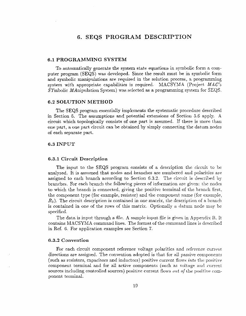
6 . SEQS PROGRAM DESCRIPTION . . . . . . . . . . . 19 6.1 PROGRAMMING SYSTEM . . . . . . . . . . . . 19

6.2 SOLUTION METHOD . . . . . . . . . . . . . . 19

6.3 INPUT . . . . . . . . . . . . . . . . . . . 19 6.3.1 Circuit Description . . . . . . . . . . . . . . 19

6.3.2 Convention . . . . . . . . . . . . . . . . 19

6.4 OUTPUT . . . . . . . . . . . . . . . . . . 20 1..

111

7 . SEQS PROGRAM APPLICATION . . . . . . . . . . . 21 7.1CASEA . . . . . . . . . . . . . . . . . . 21 7.2CASEB . . . . . . . . . . . . . . . . . . 22

8 . CONCLUSION . . . . . . . . . . . . . . . . . 25

APPENDIX A . SEQS PROGRAM LISTING . . . . . . . . . 27

8.1 SEQS SAMPLE INPUT FILE . . . . . . . . . . . . 35 REFERENCES . . . . . . . . . . . . . . . . . . 37

iv

LIST OF FIGURES

Fig. Page

1 Case A: Circuit Diagram . . . . . . . . . . . . . 21

2 Case A: SEQS Program Output . . . . . . . . . . . 22

3 Case B: Circuit Diagram . . . . . . . . . . . . . 33

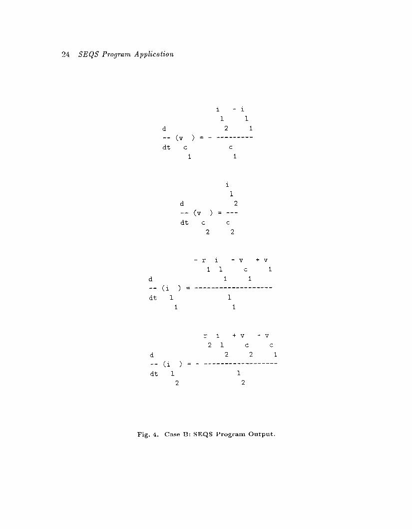
4 Case B: SEQS Program Output . . . . . . . . . . . ‘34

V

LIST OF TABLES

Table P ase

1 Case A: Circuit Description by by Branches . . . . . . . . . 21

2 Case B: Circuit Description by Branches . . . . . . . . . . 23

vii

1. INTRODUCTION

The capability of automatically generating state equations for a given system is a desirable component of an integrated environment for system control and simulation studies. A step towards the development of this capability is described in the following sections. Section 2 presents the statement of the problem to be solved. Since the solution approach involves the use of circuit analogs, network topology concepts are required; these are presented in Section 3. The governing network equations and different network formulations are given in Section 4. The problem of systematically formulating the state equations is the topic of Section 5 . A program (SEQS) developed to automatically generate the state equations is described in Section 6 and its application is illustrated in Section 7. Section 8 contains the conclusions. Appendix A gives a listing of the SEQS program and Appendix B gives a sample input file for the SEQS program.

1

2. PROBLEM STATEMENT

Given the schematic diagram of some system, for example, a nuclear power plant, it is desired to automatically generate the associated system state equations in symbolic form. These equations are used as inputs to other components of an integrated environment which may, for instance, design nonlinear optimal controllers for the system or perform numerical simulations.

A possible approach to this problem consists of two stages. First the original system schematic diagram is used to define a mathematically equivalent electric circuit. The state equations of this circuit are, by definition, the same as that of the original system. It is in this sense the circuit is the analog of the original system. Once the circuit analog is defined, it is analyzed in a systematic form to generate its state equations in symbolic form.

The first stage consists of essentially replacing different components of the original system by their circuit analogs. For each system component its associated analog may be defined in advance and stored for use in this first stage.

The concept of circuit analogs is also used in a technique known as parity simulation. Parity simulation involves the determination of a circuit analog to a physical system of interest and its construction and use to simulate the behavior of the original physical system. In recent years parity simulation has been applied to nuclear systems problems. The determination of the circuit analogs for thermal hydraulic systems, required in the first stage of state equation generation process, is discussed in Ref. 1. Related efforts are presented e l s e ~ h e r e . ~ , ~ ? ~

This work focuses on the second stage, namely, given a general electric circuit diagram find the corresponding state equations in symbolic form.

3

3. NETWORK TOPOLOGY

The concept of a graph and its use in the topological description of networks is introduced in this section. The definition of related terms is given.

A graph associated with a given a circuit diagram of an electrical network may be constructed by replacing all components by lines. Abstraction from the particular types of components that axe physically connected yields a skeleton of the network. If a reference direction is chosen for each of the lines of the graph the result is known as an oriented gruph. The lines in the graph are referred to as branches. The junction of two or more branches is known as a node or vertes. Thus graphs are composed of nodes and branches or oriented branches.

Graphs are used to describe the topological properties of networks. Topological quantities of importance in network analysis are identified in this section. The graph of a network may have more than one separate part such as the case of networks with magnetic coupling. Graphs that may be drawn on a sheet of paper without crossing lines are known as planar, otherwise they are termed nonplunar.

A node pair is simply two nodes identified for specifying a voltage varisbk. A loop or mesh is a closed path in a graph formed by a number of connected branches.

A subgraph of a given graph is formed by removing branches from the original graph. A subgraph of importance in network analysis is the tree. A tree of a connected graph (one part) of N nodes has the following properties:

1. It contains all the nodes of the graph; nodes are not left in isolated positions. 2. It contains N - 1 branches, as explained below. 3. There are no closed paths.

For a given graph there are many possible different trees. The total number is a function of the number of nodes and the number of branches in the tree. By definition, the branches removed from the graph in forming a tree are the chords or links.

An important property of a tree is the relationship between the number of nodes and the number of branches in the tree:

where: Btree = number of branches in the tree; and N = number of nodes in the tree.

This can be easily verified by constructing a tree by successively adding branches so that at each step the construct remains a tree. In other words, ncw branches are added in such a way as to never form a closed path. It is clear that each time a new branch is added exactly one new node is added. Hence Eq. (1) holds. Now the number of nodes in a tree is exactly the same as the number of nodes in the corresponding graph. Thus a tree of a connected graph is a circuitless s u b p p h of N nodes and N - 1 branches.

5

6 Network Topology

The number of chords in a graph is the difference between the total number of branches in the graph and the niunber of branches in a tree given by Eq. (1):

where: C = number of chords in the graph; B = number of branches in the graph; and N = number of nodes in the graph.

For a graph with P separate parts Eqs. (1) and (2) become

and

C = B - .€?tree = B - N + P. (4) The concept of tree is useful in determining the proper choice of current variables

for the analysis of a network.

4. NETWORK EQUATIONS

4.1 INTRODUCTION This section contains the equations that describe the behavior of networks.

Kirchhoff laws are stated and different formulations of the network equations are given including the node basis, loop basis and state variable basis formulations.

4.2 KIRCHHOFF LAWS

4.2.1 Kirchhoff Voltage Law Network equations are formulated from two simple laws first expressed by IGrch-

hoff. These laws concern the voltages around a loop and the currents entering or leaving a node.

Kirchhoff voltage law (KVL) states that the algebraic sum of all branch voltages around any closed loop of a network is zero at all instants of time. It is a consequence of the law of conservation of energy. In symbols

where: b = a branch of the network; I = a loop of the network;

b E E = all branches that belong to loop I; and (Av)b = the branch b voltage (drop or rise in the direction the loop 1 is traversed).

4.2.2 KirchhoE Current Law ICirchhoff current law (KCL) states that the algebraic sun2 of a13 branch currents

leaving any node of a network is zero at all instants of time. It is a consqiience of the law of conservation of charge. In symbols

2b = 0, for all nodes n;

where: b = a branch of the network; n = a node of the network;

b E n = all branches that belong to node n, that is, that are connected to node n; and

i b = the branch b current leaving node n.

7

8 Network Eq,uations

4.3 FORMULATIONS

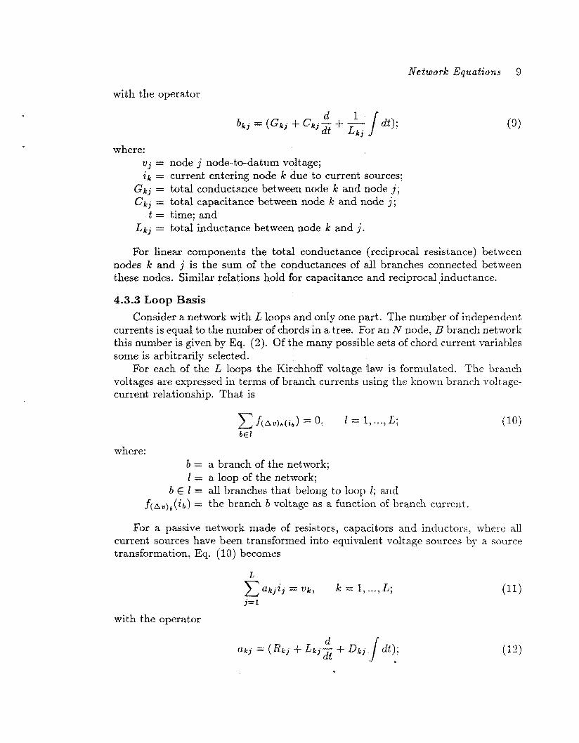
4.3.1 Introduction There is more than one possible method for the formulation of equations to

describe network behavior. Three of the most common approaches are presented in this section. ,411 methods lead to the same end result: the determination of all branch voltages and branch currents in the network. For a network with B branches this gives a total of 2B unknowns. Since the voltage-current relationship for each component is known the number of unknowns is reduced to B. That is, given the branch currents, the branch voltages may be determined, and vice versa.

Kirchhoff laws may be used to write an independent set of equations. A node is selected to be the datum or reference node.

4.3.2 Node Basis Consider a network with N nodes and only one part. The number of indepen-

dent (node pair) voltages is equal to the number of branches in a tree. For an iV node network this number is N - 1. Of the many possible node-pair variables the set of node-to-datum voltages is selected.

At each of N - 1 nodes the Kirchhoff current law is formulated. The branch currents are expressed in terms of branch voltages using the known branch voltage- current relationship. That is


b E n = a.11 branches that belong to node n, that is, that are connected to node n;

n , n' = nodes that belong to branch b; v, = node n node-to-datum voltage;

vnt = node n' node-to-datum voltage; and f ib(vn - vnj) = branch b current leaving node n as a function of branch voltage.

For a passive network made of resistors, capacitors and inductors, where all voltage sources have been transformed into equivalent current sources by a source transformation*, Ref. 5 becomes

N-1

b k j v ~ == ik, k 1, ..., N - 1; ( 8 ) 3=1

* It can be shown that a the series connection of voltage source 1,; a id resistor Rl is equivalcnt to the parallel connection of current source V;/R, and resistor A,. This is one example of a source transformation.

Network Equations 9

with the operator

where: vj = node j node-to-datum voltage; i k = current entering node k due to current sources;

G k j = total conductance between node k and node j ; c k j = total capacitance between node k and node j ;

L k j = total inductance between node k and j . t = time; and

For linear components the total conductance (reciprocal resistance) between nodes k and j is the sum of the conductances of all branches connected between these nodes. Similar relations hold for capacitance and reciprocal inductance.

4-3.3 Loop Basis Consider a network with L loops and only one part. The number of independent

currents is equal to the number of chords in a tree. For an N node, B branch network this number is given by Eq. (2). Of the many possible sets of chord current variables some is arbitrarily selected.

For each of the L loops the Kirchhoff voltage law is formiilated. The branch voltages are expressed in terms of branch currents using the known branch voltage- current relationship. That is

f ( A " ) * ( i b ) = 0, 1 = 1, *", L; b E I

where: b = a branch of the network; 1 = a loop of the network;

b E I = all branches that belong to loop I; and f ( A v l b ( i b ) = the branch b voltage as a function of bra.nch current.

For a passive network made of resistors, capacitors and inductors, where all current sources transformation,

with the operator

have been transformed into equivalent voltage sources by a source Eq. (10) becomes

L

j = 1

(12)

10 Network Equutions

where: i j = branch j current; V k = total voltage rise dong loop k due to voltage sourees;

&j = total resistance common to loops k and j ; L k j = total inductance common to loops k and j ;

Dkj = total elastance (reciprocal capacitance) common to loops k and j . t = time; and

For linear components the total resistance of a loop is the sum of the resistances of all branches that form the loop. Similar relations hold for inductance and elast ance.

4.3.4 State Variable Basis The

state variables usually selected for network analysis are the capacitor voltages and inductor currents. These replace node-to-datum voltages and loop currents in the two previous formulations. Knowledge of the state variables permits determination of all other network voltages and currents.

The state variable formulation is especially suited for describing systems in general, including time-varying and nonlinear systems. The resulting form is par- ticularly appropriate for the computer simulation of the system. 'This formulation is covered in detail in the following section.

A third formulation of network equations is that using state variables.

5. SYSTEMATIC FORMULATION O N A STATE VARIABLE BASIS

To write network equations in state variable form a systematic procedure must be developed. The description of the developed procedure follows. -4 number of applicable conditions and the solution sequence are presented. Assumptions and possible extensions axe discussed. Finally an alternate procedure is mentioned.

A network of one part, N nodes, B branches and C chords is assumed.

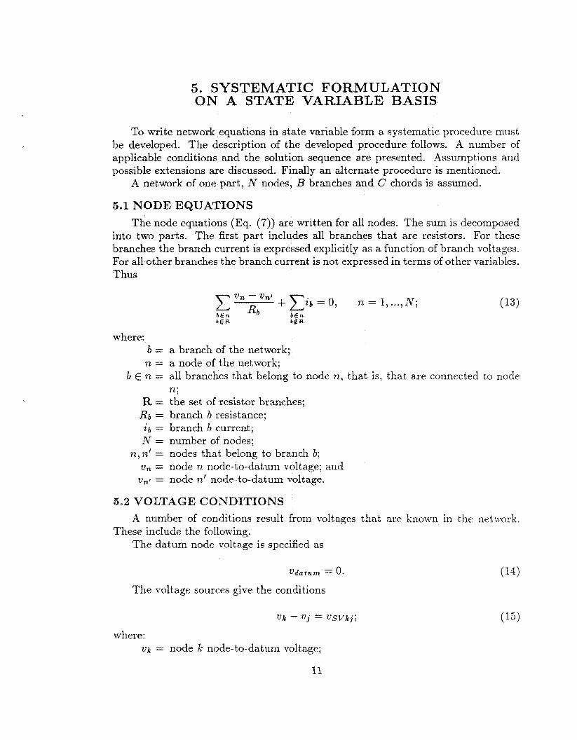
5.1 NODE EQUATIONS The node equations (Eq. (7)) are written for all nodes. The sum is decomposed

into two parts. The first part includes all branches that are resistors. For these branches the branch current is expressed explicitly as a function of branch voltages. For all other branches the branch current is not expressed in terms of other variables. Thus

c On ,.""' + Gib = 0, n = I, ..., N ;


b E n = all branches that belong to node n, that is, that are connected to node n;

R = the set of resistor branches; Rb = branch b resistance;

i b = branch b current; N = number of nodes;

un = node n node-to-datum voltage; and v,r = node n' node-to-datum voltage.

n, rz' = nodes that belong to branch b;

5.2 VOLTAGE CONDITIONS

These include the following. A number of conditions result from voltages that are known in the network.

The datum node voltage is specified as

The voltage sources give the conditions

where: vh = node k node-to-datum voltage;

11

12 Systematic Formulation on a State Variable Basis

vj = node j node-to-datum voltage; and V s V k j = voltage determined by the source connected between nodes k and j .

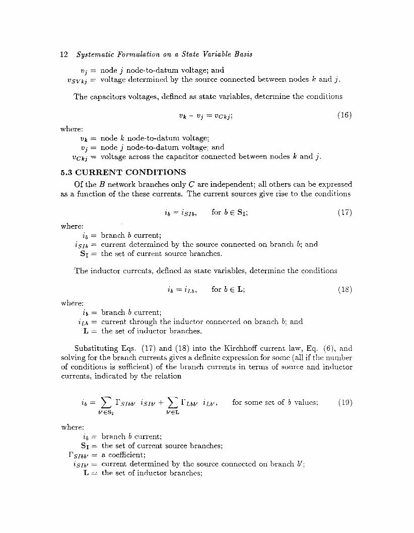
The capacitors voltages, defined as state variables, determine the conditions

v k - v j = V C k j ; (16) where:

v k = node k node-to-datum voltage; v j = node j node-to-datum voltage; and

V C k j = voltage across the capacitor connected between nodes k and j .

5.3 CURRENT CONDITIONS Of the B network branches only C are independent; all others can be expressed

as a function of the these currents. The current sources give rise to the conditions

where: i b = branch b current;

SI = the set of current source branches. i s r b = current determined by the source connected on branch b; and

The inductor currents, defined as state variables, determine the conditions

i b = i r , b , for b E L; (18) where:

i b = branch b current;

L = the set of inductor branches. zr,b = current through the inductor connected on branch b; and

Substituting Eqs. (17) and (18) into the Kirchhoff current law, Eq. (6), and solving for the branch currents gives a definite expression for some (all if the number of conditions is sufficient) of the branch currents in terms of source and inductor currents, indicated by the relation

branch b current; the set of current source branches; a coefficient; current determined by the source connected on branch b’; the set of inductor branches;

Systematic F o r m u h t i o n o n a State Variable Basis 13

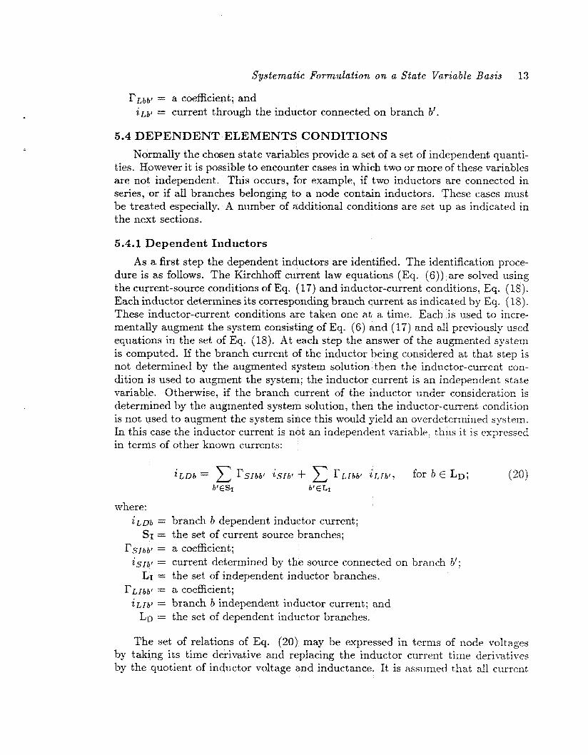
r L b b ’ = a Coefficient; and i L b ’ = current through the inductor connected on branch h’.

5,4 DEPENDENT ELEMENTS CONDITIONS Normally the chosen state variables provide a set of a set of independent quanti-

ties. However it is possible to encounter cases in which two or more of these variables are not independent. This occurs, for example, if two inductors are connected in series, or if all branches belonging to a node contain inductors. These cases must be treated especially. A number of additional conditions are set up as indicated in the next sections.

5.4.1 Dependent Inductors As a first step the dependent inductors are identified. The identification proce-

dure is as follows. The Kirchhoff current law equations (Eq. ( 6 ) ) are solved using the current-source conditions of Eq. (17) and inductor-current conditions: Eq. (18). Each inductor determines its corresponding branch current as indicated by Eq. (18). These inductor-current conditions are taken one at a time. Each is used to incre- mentally augment the system consisting of Eq. (6) and (17) and all previously used equations in the set of Eq. (18). At each step the answer of the augmented system is computed. If the branch current of the inductor being considered at that step is not determined by the augmented system solution then the inductor-current condition is used to augment the system; the inductor current is an independent state variable. Otherwise, if the branch current of the inductor under consideration is determined by the augmented system solution, then the inductor-cument condition is not used to augment the system since this would yield an overdetermined system. In this case the inductor current is not an independent variable, thus it is espressed in terms of other known currents:

where : iLDb = branch b dependent inductor current; SI = the set of current source branches;

rsrbf,’ = a coefficient; iSIb’ = current determined by the source connected on branch b’;

LI = the set of independent inductor branches.

i L I b j = branch b independent inductor current; and r L l b b ’ = a coefficient;

LD = the set of dependent inductor branches.

(20)

The set of relations of Eq. (20) may be expressed in terms of node voltages by taking its time derivative and replacing the inductor current time derivatives by the quotient of inductor voltage and inductance. It is assumed that all current

14

source coefficients are zero or that current source time derivatives are negligible. The result is

Systematic Formulation on a State Variable Basis

where : n+(b) == the positive node of branch b; u,+(b) = node n+(b) node-to-datum voltage; n-(b) = the negative node of branch b; v,- (a) = node n-(b) node-to-datum voltage;

n+(b’) = the positive node of branch b‘; vn+(bt) = node n+(b’) node-to-datum voltage; n-(b’) = the negative node of branch b’; v n - ( b t ) = node n-(b’) node-to-datum voltage; and

Lb = branch b inductance;

L b l = branch b’ inductance.

Equation (21) is an additional relation to enable determination of node voltages.

5.4.2 Dependent Capacitors Dependent capacitors occur? for example, if two or more are connected in parallel

or in the case of capacitor loops. A treatment similar to the dependent inductors case can be developed. The end result is a linear combination of branch currents where the coefficients depend on the dependent capacitances. For practical nuclear systems the capacitor loop case is unlikely to occur. The case of capacitors in parallel can be avoided by an appropriate construction of the circuit analog. For these practical reasons no further consideration is given to the dependent capacitor case.

5.5 SOLUTION PROCEDURE The previous sections contain the various conditions that must be satisfied in

the network. The solution procedure consists of the following steps. First a system is assembled iising the node cqimtions, Eq. (13), and the voltage conditions, Eqs. (14), (15), and (16). The current condition, Eq. (19)7 is used to substitute the right hand side of Eq. (19) for its left hand side in the initial system of equations. The resulting system is augmented by the dependent inductor conditions. Ecl. (21). Any remaining branch currents are subsequently eliminated and finally the system is solved for the node voltages at all nodes:

vn 7 for n = 1, ..,, N . (22)

The next step consists of writing the state equations using previously stated relations. For capacitors the state equat.ion is

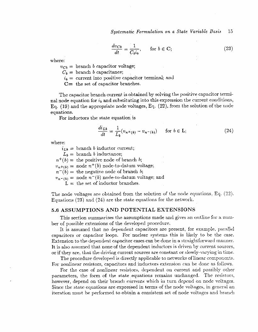
Systematic Formulation on a State Variable Basis 15

where: VCb = branch b capacitor voltage; Cb = branch b capacitance;

i b = current into positive capacitor terminal; and C= the set of capacitor branches.

The capacitor branch current is obtained by solving the positive capacitor terminal node equation for i b and substituting into this expression the current conditions, Eq. (19) and the appropriate node voltages, Eq. (22), from the solution of the node equations.

For inductors the state equation is

where: i L b = branch b inductor current; Lb = branch b inductance;

n+(b) = the positive node of branch b; vn+(b) = node n+(b> node-to-datum voltage; n-(b) = the negative node of branch b; nn-(b) = node n-(b) node-to-datum voltage; and

L = the set of inductor branches.

The node voltages are obtained from the solution of the node equations, Eq. (22). Equations (23) and (24) are the state equations for the network.

5.6 ASSUMPTIONS AND POTENTIAL EXTENSIONS This section summarizes the assumptions made and gives an outline for a num-

ber of possible extensions of the developed procedure. It is assumed that no dependent capacitors are present, for example, parallel

capacitors or capacitor loops. For nuclear systems this is likely to be the case. Extension to the dependent capacitor cases can be done in a straightforward manner. It is also assumed that none of the dependent inductors is driven by current sources, or if they are, that the driving current sources are constant or slowly-varying in time.

The procedure developed is directly applicable to networks of linear components. For nonlinear resistors, capacitors and inductors extension can be done as follows.

For the case of nonlinear resistors, dependent on current and possibly other parameters, the form of the state equations remains unchanged. The resistors, however, depend on their branch currents which in turn depend on node voltages. Since the state equations are expressed in terms of the node voltages, in general an iteration must be performed to obtain a consistent set of node voltages and branch

16 Systematic Formulation o n a State Variable Basis

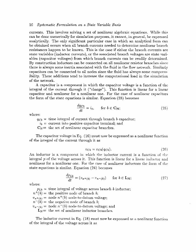
currents. This involves solving a set of nonlinear algebraic equations. While this can be done numerically for simulation purposes, it cannot, in general, be expressed analytically. The only significant particular case in which an analytical form can be obtained occurs when all branch currents needed to determine nonlinear branch resistances happen to be known. This is the case if either the branch currents are state variables (inductor currents), or the associated branch voltages are state variables (capacitor voltages) from which branch currents can be readily determined. By construction inductors can be connected on all nonlinear resistor branches since there is always some inertia associated with the fluid in the flow network. Similarly capacitors can be connected to all nodes since the fluid has always some compress- ibility. These additions tend to increase the computational load in the simulation of the network.

A capacitor is a component in which the capacitor voltage is a function of the integral of the current through it (“charge”). This function is linear for a linear capacitor and nonlinear for a nonlinear one. For the case of nonlinear capacitors the form of the state equations is similar. Equation (23) becomes

for b E CN; dqCb . -- - a b , d t

where: qCb = time integra.1 of current through branch b capacitor;

CN= the set of nonlinear capacitor branches. i b = current into positive capacitor terminal; and

The capacitor voltage in Eq. (16) rnwt now be expressed as a nonlinear function of the integral of the current through it as

V C b = vCb( Q C b ) . (26) ,4n inductor is a component in which the inductor current is a function of the integral p of the voltage across it. This function is linear for a linear inductor and nonlinear for a nonlinear one. For the case of nonlinear inductors the form of the state equations is similar. Equation (24) becomes

for b E LN; where:

P L b = time integral of voltage across branch b inductor; n+(b) = the positive node of branch b; 2),+(b) = node n+(b) node-to-datum voltage; n-(b) = the negative node of branch b; vn-(b) = node n - ( b ) node-to-datum voltage; and

Lx= the set of nonlinear inductor branches.

(27)

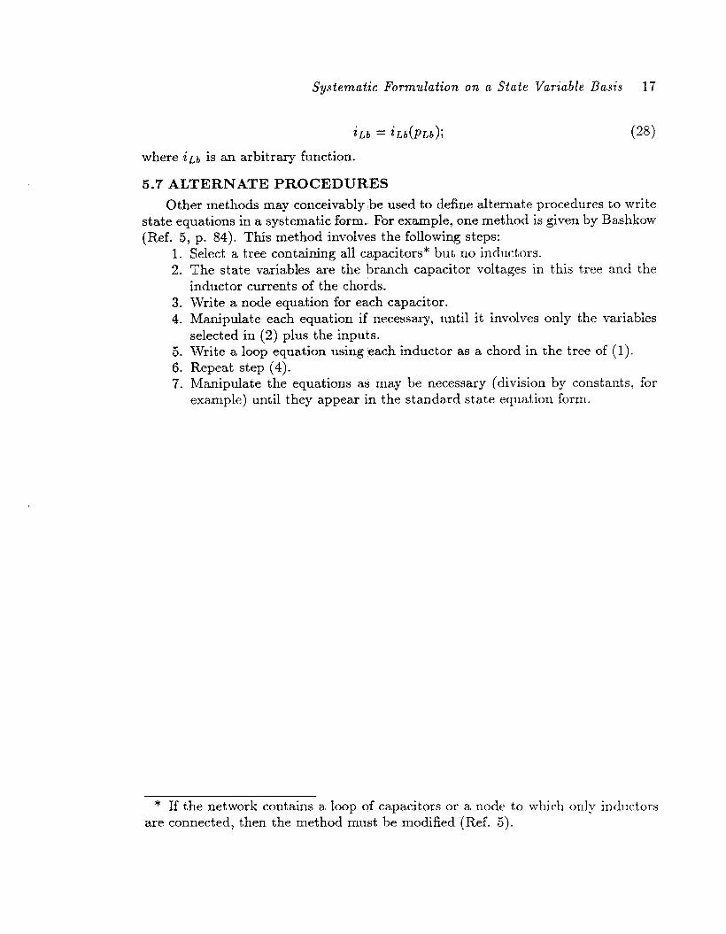
The inductor current in Eq. (18) must now be expressed as a nonlinear function of the integral of the voltage across it as

~ y s t e m a t i c Formulafaon on a State Variable Basis 17

where i ~ b is an arbitrary function.

5,.7 ALTERNATE PROCEDURES Other methods may conceivably be used to define alternate procedures to write

state equations in a systematic form. For example, one method is given by Bashkow (Ref. 5, p. 84). This method involves the following steps:

1. Select a tree containing all capacitors* but no inductors. 2. The state variables are the branch capacitor voltages in this tree and the

3. Write a node equation for each capacitor. 4. Manipulate each equation if necessary, until it involves only the variables

5. Write a loop equation using each inductor as a chord in the tree of (1). 6. Repeat step (4). 7. Manipulate the equations as may be necessary (division by constants, for

inductor currents of the chords.

selected in (2) plus the inputs.

example) until they appear in the standard state equation form.

* If the network contains a loop of capacitors or a node to which only inductors are connected, then the method must be modified (Ref. 5 ) .

6 . SEQS PROGRAM DESCRIPTION

6.1 PROGRAMMING SYSTEM

To automatically generate the system state equations in symbolic form a computer program (SEQS) was developed. Since the result must be in symbolic form and symbolic manipulations are required in the solution process, a programming system with appropriate capabilities is required. MACSYMA (Project M A C’s Symbolic MAnipulaticsn System) wits selected as a programming system for SEQS.

6.2 SOLUTION METHOD

The SEQS program essentially implements the systematic procedure described in Section 5 . The assumptions and potential extensions of Section 5.6 apply. A circuit which topologically consists of one part is assumed. If there is more than one part, a one part circuit can be obtained by simply connecting the datum nodes of each separate part.

6,3 INPUT

6.3.1 Circuit Description

The input to the SEQS program consists of a description the circuit to be analyzed. It is assumed that nodes and branches are numbered and polarities are assigned to each branch according to Section 6.3.2. The circuit is described by branches. For each branch the following pieces of information are given: the nodes to which the branch is connected, giving the positive terminal of the branch first, the component type (for example, resistor) and the component name (for example, R3). The circuit description is contained in one matrix, the description of a branch is contained in one of the rows of this matrix. Optionally a datum node may be specified.

The data is input through a file. A sample input file is given in -4ppendix B. It contains MACSYMA command lines. The format of the command lines is described in Ref. 6. For application examples see Section 7.

6.3.2 Convention

For each circuit component reference volt age polarities and reference current directions are assigned. The convention adopted is that for all passive Components (such as resistors, capacitors and inductors) positive current flows into the positive component terminal and for all active components (such as voltage and current sources including controlled sources) positive current flows out of the positive component terminal.

19

SEQS Pr0gra.m Description 20

6.4 OUTPUT The output of the SEQS program is the list of the system state equations in

symbolic form. This list is output to the terminal and saved for further symbolic manipulations in the MACSYMA environment.

7. SEQS PROGRAM APPLICATION

b

1 2 3 4 5 6

To illustrate the application of the SEQS program two cases are presented in this section.

n+ n- component component t Y Pe name

1 2 C C1 2 3 R rl 3 4 R 7-2 4 1 C c2 3 5 R 7-3 5 1 C c3

7.1 CASE A As a first case of the application of the SEQS program consider the circuit

of Fig. 1. In Fig. 1 nodes and branches are numbered arbitrxily, with branch numbers given in parenthesis. Using the numbering indicated in Fig. 1 the circuit description matrix is farmed; the result is shown in Table 1. In Table 1 a branch is indicated by b while nf and n- refer to the associated nodes. With the information of Table 1 an input file is prepared. For this case the input file is the one given in Appendix B. The SEQS program generates the equations given in Fig. 2. The result of Fig. 2 may be verified by a hand calculation of the state equations.

1

Fig. 1. Case A: Circuit Diagram.

Table 1: Case A: Circuit Description by Branches.

21

22 SEQS Program Application

r v + r v +(r + r ) v 2 c 3 c 3 2 c

d 3 2 1

dt c ( c r + c r ) r + c r r 1 1 2 1 1 3 1 . 1 2

Fig. 2. Case A: SEQS Program Output.

7.2 CASE B Consider the circuit of Fig. 3. In Fig. 1 nodes and branches are numbered

with branch numbers given in parenthesis. Using the nunbering given in Fig. 3 the circuit description matrix is formed; the result is shown in 'Table 2. In Table 2 b indicates the branch, and n+ and n- the associated nodes. With the input of Table 2 the SEQS program generates the equations given in Fig. 4. The result of Fig. 4 may be verified by a hand calculation of the state equations.

SEQS Program Application 23

1

Fig. 3. Case B: Circuit Diagram.

Table 2: Case B: Circuit Description by Branches.

24 SEQS Program Applicataon

i - i 1 1

d 2 1

dt c C

_ _ ( v ) = - ---------

1 1

i 1

d 2 _- (v ) = --- dt c C

2 2

- r i - v + v 1 1 C 1

d 1 1 _ _ (1 ) = ------------------- dt 1 1

1 1

Fig. 4. Case B: SEQS Program Output.

8. CONCLUSION

A step towards the development of the capability of automatically generating state equations for a given system is described. The solution approach involves the use of circuit analogs. The different network formulations are discussed. The state equation formulation and a systematic implementation procedure is addressed. Potential extensions of this procedure are outlined. A program (SEQS) is developed to automatically generate the state equations. Results of the application of the SEQS program are given for illustrative cases.

25

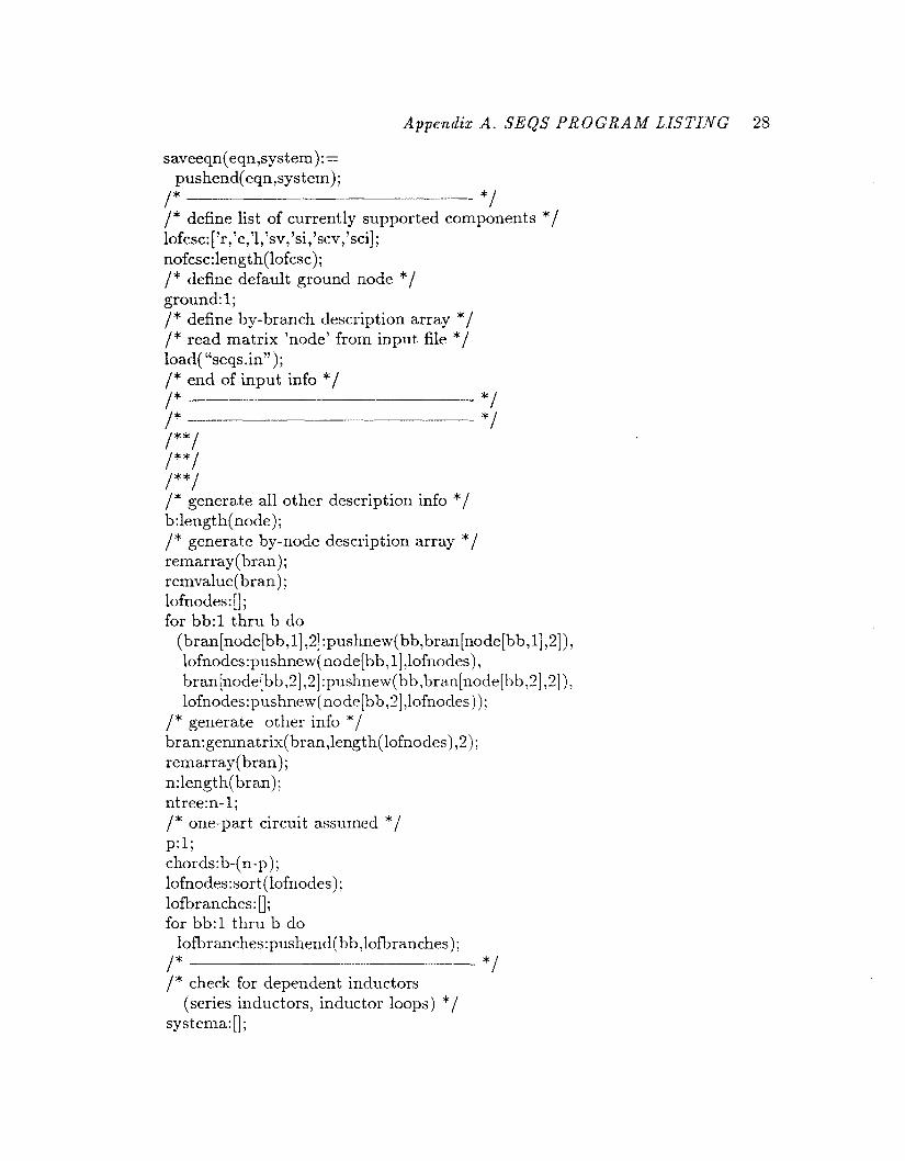
APPENDIX A. SEQS PROGRAM LISTING

This Appendix contains the listing of the SEQS program.

/* - * / /**I /**I /**I /* Symbolic State Equation Generator for a Circuit */ /* SEQS Program */ /* 8-SET-1988 Version */ /* File 'seqs.mac' */ I**/ /**I /**I /* - * / /* define auxiliary functions first */ /* define auxiliary function pushnew */ pushnew(elem,list):=

if (listp(1ist)) then (if (not member(elern,list)) then

list:cons(elem,list )

list)

[elem];

else

else

/* define auxiliary function pushend */ pushend(elem,lis t ) : =

if (Pistp(1ist)) then (if (not member(elem,list)) then

list :endcons( elem,list) else list)

[elem]; else

/* define auxiliary function makealist */ makealist (list ,filter) :=

(for bb:l thru b do if(mernber(node[bb,3] ,filter)) then

Bist:pushend( bb,list), list);

/* define auxiliary function saveeqn */

Appendix A. SEQS PROGRAM LISTING 28

saveeqn(eqn,system): = pushend( eqn’system) ;

- */ .... /* /* define list of currently supported components */ lofcsc: [’ r , ’c,’l,’sv,’si, ’ scv, ’sci] ; nofcsc:length( lofcsc); /* define default ground node */ ground: 1 ; /* define by-branch description array */ /* read matrix ’node’ from input file */ load( “seqs.in”); /* end of input info */

*/ /* _____ /* - * / /**I /**/ /**/ /* generate all other description info */ b:length(node); /* generate by-node description array */ remarray (bran); remvaluet bran); lofnodes:[]; for bb:l thru b do

(bran [node [ bb ) 1],2] :pus hnew( b b, bran [node [ bb , 1],2]), lofnodes:pushnew( node[bb,l],lofnodes), bran [node[ bb ’31 ,2] :pushnew( bb ,bran[node[bb ,3] ,2] ) ) lofnodes: pushnew (no de [ bb ,3] Jofnodes ) ) :

/* generate other info * / bran:genmatrix( bra,n,length(lofnodes) J); remarray( bran) ; n:length( bran); ntreen- 1; /* one-part circuit assumed */ p:l; chords:b-( n-p); lofnodes:sort( lofnodes); lofbranches: [I; for bb:l thru b do

lofbranches:pushend( bb,lofbranches); */ ......._. /*

/* check for dependent inductors

systems:[]; (series inductors, inductor loops) */

29 Appende‘z A . SEQS PROGRAM LISTING

for nn:l thru n do (sum:O, for bb in bran[nn,2] do

(if (nn=node[bb,l]) then alpha:+l, if (nn=node[bb,2]) then alpha:-1, sum:sum+alpha*i [ bb]),

eqn:sum=O, systema:saveeqn(eqn,sys tema));

/* solve systema for {i[b]} */ lofcurrents: 1; for bb:l thru b do

lofcurrents:pushend(i [bb] Jofcurrents); solve( sys tema Jofcurrent s) ; /* make list of (real) current sources */ lofrcsources: [I ; lofr csources :make alis t ( lofr csources , [‘si, ’sci] ) ; /* make list of inductors */ lofinductors: [I; lofinduct ors:makealist (lofinductors, [ ’1] ) ; /* process list of (real) current sources */ s ys tema 1 : [I ; for bb in lofrcsources do

/* recompute answer from augmented system */ /* reset counter */ (%rnum:O, temp:solve(append(systema,systemal) Jofcurrents), /* is i[b] free? */ if (not apply( ’freeof,

endcons( part (temp ,1 ,bb) ,%rnuxnlist) j then /* Yes */ (eqn:i[bb]=isource[bb], systemal :saveeqn(eqn,systemal))

/* no */ (print( “inconsistent current source specification: ,”

bb7

else

current source on branch,” Lf

“attempts to impose a current,” “already determined as: ,” Idisplay( part (temp,l ,bb))),

/* stop */ error( ’errorl)));

/* process list of inductors */ lofindinductors: [I ;

A p p e n d i x A . SEQS PROGRAM LISTING 30

lofdepinductors: [I; lofindindbran: 1 ; lofdepindbran: [I ; for bb in lofinductors do

/* recompute answer from augmented system */ /* reset counter */ (%rnum:O, t emp:solve( append( sys t enia,sys t e n d ) Jofcurrent s) , /* is i[b] free? */ if (not apply( ’freeof,

endcons(part (tenip,l ,bb) ,%rnumlist ))) then /* Yes */ (eqn:i[bb]=isource[bb], systemal:saveeqn( eqn,systemal), lofindinductors: saveeqn( eqn ,lo findinduct ors) , lofindindbr an: pushend( bb ,lofindindbr an) )

else /* no */ (eqn:part (temp,l ,bb), lofdepinductors:saveeqn( eqnJofdepinductors) , lofdepiIidbran:pushend( bb’lofdepindbran)));

.. */ /* /* define current-source conditions */ systemcurr: [I; /* recompute final answer from augmented system */ /* reset counter */ % rnum : 0 ; temp:solve( append( sys tema,sys temal ) Jofcurrent s); for eqn in part(temp,l) do

/* is i[b] free? * / (if (not apply( ’freeof,

endcons(eqn,%rnum-list))) then /* yes: do nothing */ c1

else /* no: save equation */ systemcurr: saveeqn( eqn ,s ys t emcurr));

I**/ I**/ /* make list of resistors * / lofresistors:[]; lofresistors:niakeaIist(lofresistors, [’r]); 1ofacsources:lofresistors; if systemcurr=[] then

31 Appendix A . SEQS PROGRAM LISTING

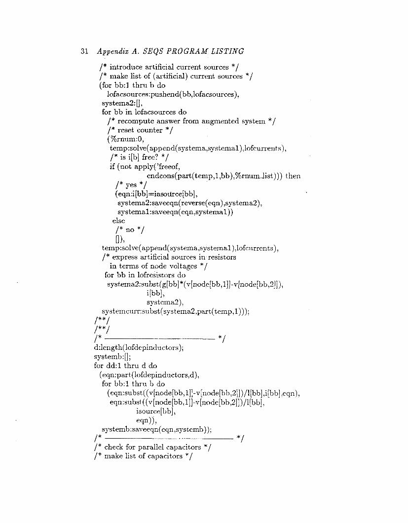
/* introduce artificial current sources */ /* make list of (artificial) current sources */ (for bb:l thru b do

systema2: [I, for bb in lofacsources do

lofacsources:pushend( bbJofacsources),

/* recompute answer from augmented system */ /* reset counter */ (%rnum:O, temp:solve( append(systema,systemal),lofcurrent s), /* is i[b] free? */ if (not apply(’freeof,

endcons( part( t emp, 1 ,bb),%rnumlist ))) then /* Yes */ (eqn:i[bb]=iaso~irce[bb] , sys tem&:saveeqn( reverse( eqn) ,sys tema2)) systemal :saveeqn( eqn,systemal))

else /* no */ [ I > ?

temp: solve( append( sys tema,sy s temal ) Jofcurren t s) , /* express artificial sources in resistors

for bb in lofresistors do in terms of node voltages */

systema2:subst(g[bb] *( v[node[bb,l J J -v[node[bb,2]]), i bbl, systema2),

sys t emcurr: subst (s y s t ema2 ,part (temp, 1))); /**/ /**/ I* *I d :lengt h( lofdepinduc t ors ) ; systemb: [] ; for dd:l thru d do (eqn:part(lofdepinductors,d), for bb:l thru b do

( eqn: subs t ( ( v[node[b b , l]]-v[ node [bb ,211) /1[ bb] ,i [ b b] ,eqn) , eqn:subst (( v [node[bb, l]]-v[node[bb72]])/l[bb],

isource[bb],

systemb:saveeqn( eqn,sys temb));

/* check for parallel capacitors */ /* make list of capacitors */

esn)),

/* - */

Appendix A . SEQS PROGRAM LISTING 32

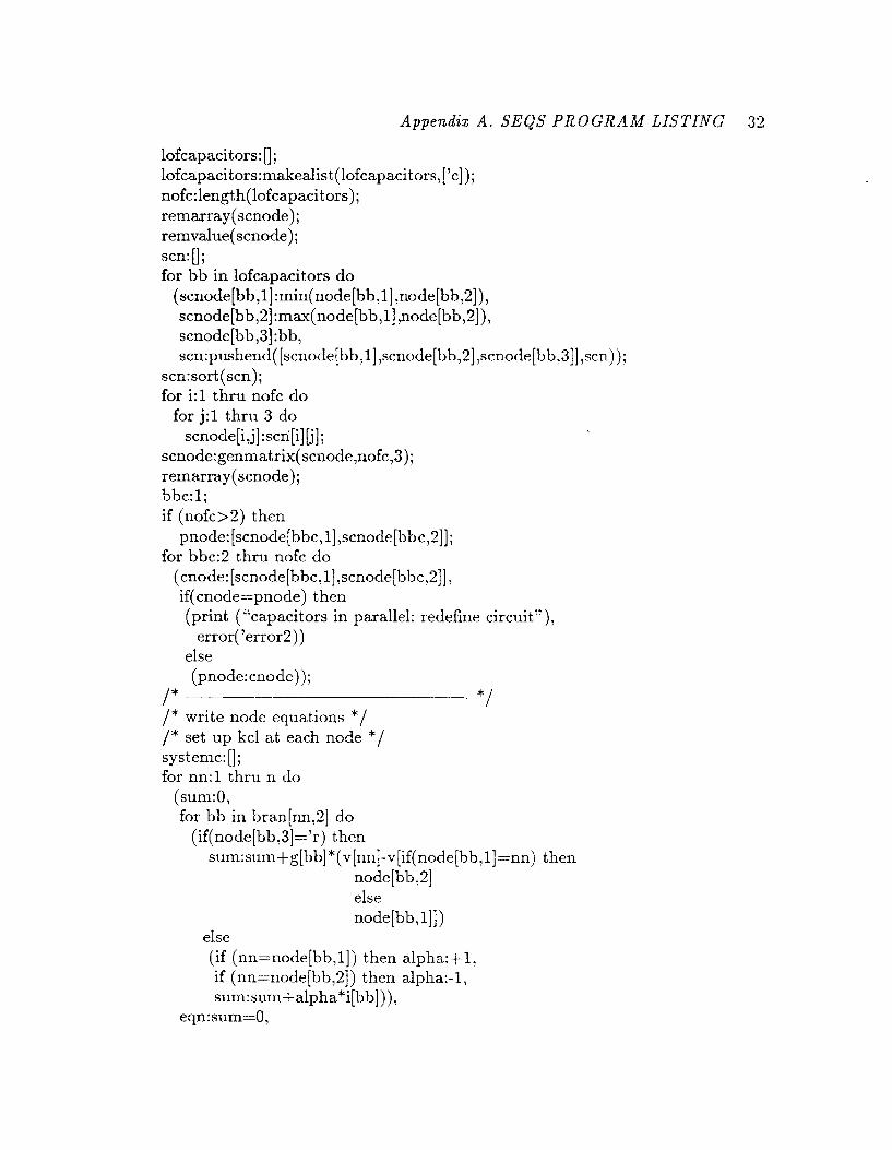
lofcapacitors: [I; lofcapaci tors:makealist (lofcapacitors, [ ’c] ); nofc:length( lofcapacitors); remarray( scnode); remvalue( scnode); scn: [I; for bb in lofcapacitors do

(scnode[bb,l] :min( node[ bb,l] ,node[bb,2]), scnode[bb,2]:max(node[bb,l] ,node[bb,Z]), scnode[ bb ,3] : bb, scn: pushend( [ scnode[ bb , 11 ,scnode [ bb ,2] ,scnode [ b b ,311 ,scn) ) ;

scn:sort(scn); for i:l thru nofc do

for j:1 thru 3 do scnode [i ,j] : scri [i] [j] ;

scnode:geximatrix( scnode,nofc,3); remarray( scnode); bbc:l; if (nofc>2) then

for bbc:2 thru nofc do pnode: [scnode[bbc, 11 ,scnode[bbc,2]] ;

(cnode: [scnode [bbc, 11 ,scnode[ bbc,2]] , if( cnode=pnode) then (print (“capacitors in parallel: redefine circuit”),

else error( ’error2))

(pnode:cnode)); - */ _- /”

/* write node equations */ /* set up kcl at each node */ systemc:[]; for nn:l thru n do

(sum:O, for bb in bran[nn,2] do

(if( nocle[bb ,3]= ’r ) then sum: siim+g [bb] * (v[nn]-v[if( node[bb, 11 =nn) then

node[bb,2] else node [ bb, 111)

else. (if (nn=node[bb,l]) then alpha:+l, if (nn=node[bb,Z]) then alpha:-1, sum:sum+alpha*i[l-)b])),

eqn: sum=O,


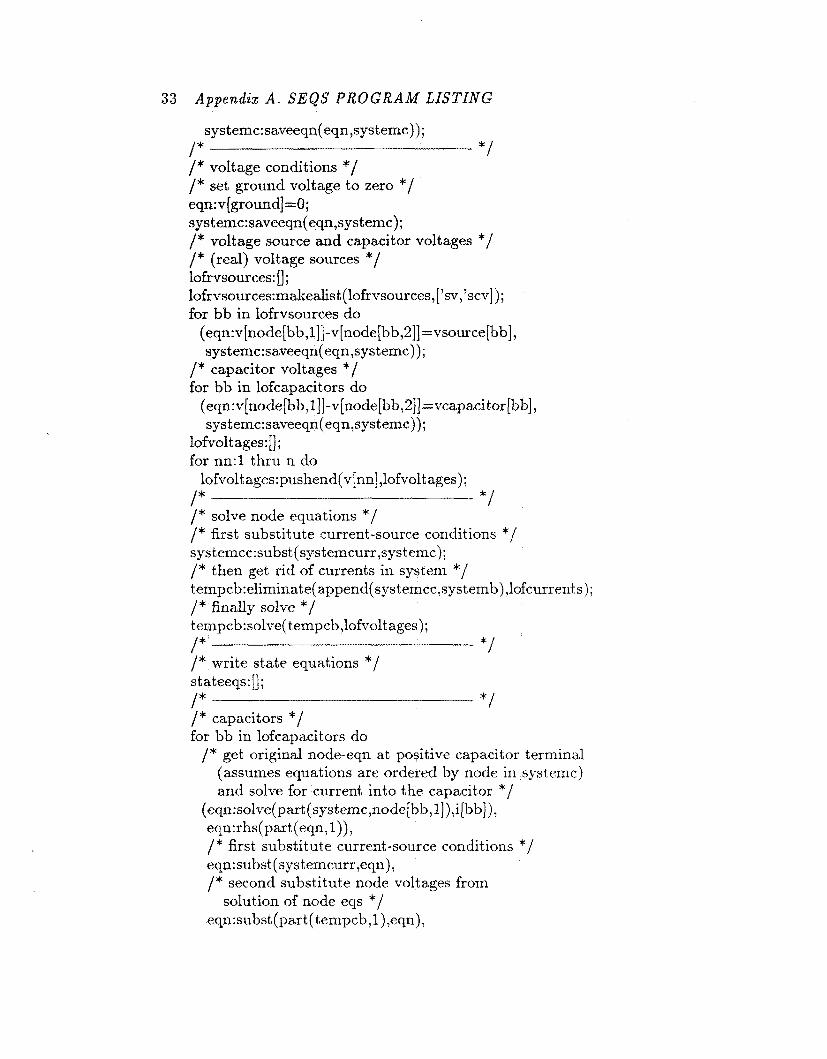
systemc:saveeqn(eqn,systemc)); /* - */ /* voltage conditions */ /* set ground voltage to zero */ eqn:v[groundJ =O; systemc:saveeqn(eqn,systemc); /* voltage source and capacitor voltages */ /* (red) voltage sources */ lofrvsources: u ; 1ofrvsources:makeaLst (lofrvsources, ['sv,'scv] ); for bb in lofrvsources do

(eqn:v[node[ bb,l]] -v[node[b b ,211 =vsource [bb] , systemc:saveeqn( eqn,systemc));

/* capacitor voltages */ for bb in lofcapacitors do

(eqn:v{node[ bb,l]]-v[node[bb, 211 Evcapaci t or [ bb] , systemc:saveeqn( eqn,systemc));

lofvol t ages: [] ; for nn:l thru n do

lofvoltages:pushend( v[nn] ,lofvoltages); /* - * / /* solve node equations */ /* first substitute current-source conditions */ sys t emcc: subst( sys t emcurr ,s ystemc); /* then get rid of currents in system */ tempcb: eliminat e( append( sys temcc, sys temb) Jofcurrent s ) ; /* finally solve */ tempcb: solve( t empcb ,lofvol t ages); /* - */ /* write state equations */ st ateeqs: [I;

*/ /* /* capacitors */ for bb in lofcapacitors do

__-

/* get original node-eqn at positive capacitor terminal (assumes equations are ordered by node in systemc) and solve for current into the capacitor */

(eqn:solve( pad (s ys t emc,node [ b b ,1] ) ,i [b b] ) , eqn:rhs( part (eqn, I)), /* first substitute current-source conditions */ eqn:subst (s yst emcurr,eqn), /* second substitute node voltages from

solution of node eqs */ eqn:subst( part (tempcb, l),eqn),

Appendis A . SEQS PROGRAM LISTING 34

eqn: 'diff (vcapacit or [ bb] , t ) = ( 1 /c [b b] ) *eqn, stateeqs:saveeqn( eqn,st ateeqs));

*I /* ___________ ~- /* inductors */ for bb in lofinductors do (eqn:'diff(iinductor[bb],t)=( l/l[hb])*

(part (t empcb, 1 ,node[bb, 11'2) -part(tempcb,l,node[bb,Z] ,2)),

stateeqs:saveeqn(eqn,st ateeqs)); .I_____. - */ /*

/* make final substitutions */ sst ateeqs: [I ; for eqn in stateeqs do

(eqnl :eqn, for bb in lofinductors do (eqnl:subst(iinductor[bb] ,i[bb] ,eqnl), eqnl:subst( iinductor[bb] ,isource[bb] ,eqnl)),

sst at eeqs:saveeqn( eqnl ,sst at eeqs)); /* put in desired form */ for bb in lofresistors do

/* change na.mes */ /* make list of (independent) voltage sources */ lofsvsources: [I ; lofsvsources:makealist(lofsvsoiirces, ['sv]); /* make list of controlled voltage sources */ lofscvsources: 0 ; lofscvsources:makealist (lofscvsources , ['scv] ); for bb in lofsvsources do

ss t ateeqs: subst (sv [ h b] ,vsource [b b] , sst ateeqs) ; for bb in lofscvsources do

sstateeqs:subst( scv[bb] ,vsource[bb],sstateeqs); /* make list of (independent) current sources */ lofsisources: [I ; lofsisources:makealist (lofsisources '['si]); /* make list of controlled current sources */ lofscisources: [I ; 1ofscisources:makealist (lofscisources, ['sci]); for bb in lofsisources do

for bb in lofscisources do

ss tat eeqs:subst ( 1 /r [bb] ,g [bb] ,sst ateeqs) ;

sstateeqs:suhst (si [bb] ,isource[bb] 'sstateeys);

sstateeqs:subst (sci[bb] ,isource[bb] ,sstateeqs); /**/ for bb:l thru b do


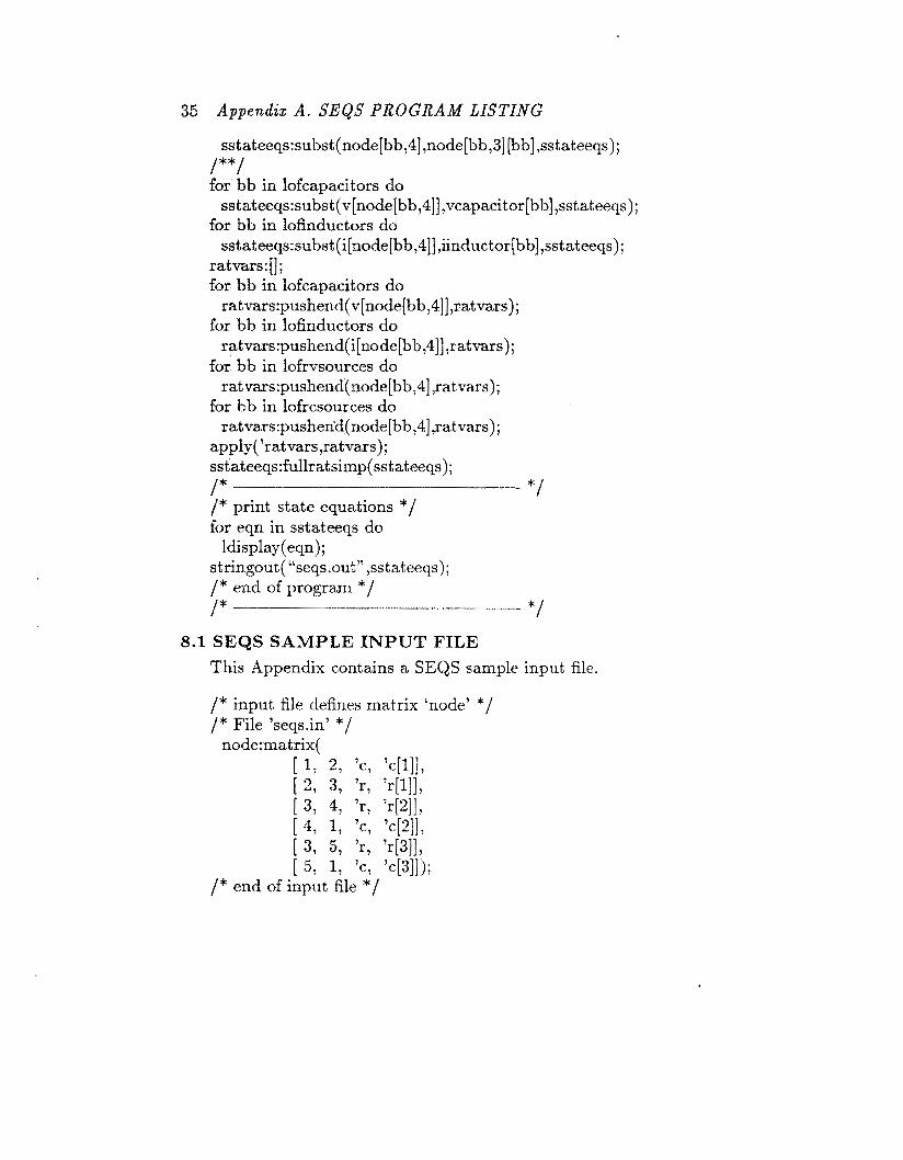
sstateeqs:subst (node[ bb ,4] ,node [ bb ,3] [bb] ,sst ateeqs ) ; /**/ for bb in lofcapacitors do

for bb in lofinductors do

rat~rc~-rs:[] ; for bb in lofcapacitors do

for bb in lofinductors do

for bb in lofrvsourees do

for bb in lofrcsources do

apply( 'ratvars,ratvars); sst ateeqs:fullratsirnp( sst ateeqs);

/* print state equations */ for eqn in sstateeqs do

stringout ( "seqs.out" ,sstat eeqs) ; /* end of program */

sstateeqs:subst (v[node[bb,4]] ,vcapacitor[bb] ,sstateeqs);

sstateeqs:subs t (i [node[bb,$]] ,iinductor [ bb] ,ss tat eeqs ) ;

ratvars:pushend( v[node[bb ,411 ,ratvars);

ratvars:pushend(i[node[bb74]] ,ratvars);

rat vars:pushend( node[bb,4] ,ratvan);

ratva.rs:pushen'd( node[bb,4] ,ratvars) ;

/* */

Idisplay( eqn);

/* - - */ 8.1 SEQS SAMPLE INPUT FILE

This Appendix contains a SEQS sample input file.

REFERENCES

1. Depiante, E. V., “Parity Simulation of Light Water Reactor Thermal Hydraulics,” Ph. D. Thesis, Dept. of Nucl. Eng., M.I.T. (May 1988).

2. Laughton, P. J., “Parity Simulation Applied to Reactor Physics Nodal Thcory Transient Analysis,” Ph. D. Thesis, Dept. of Nucl. Eng., M.I.T. (December

3. Lam, J.-T., “Parity Simulation of the Boiling-Pot, A Specific Two-Phase Flow System,” S. B. Thesis, Dept. of Electrical Eng., M.I.T. (May 1986).

4. Mweene, L. H., “Parity Simulation of Two-Phase Hydraulic Flow with Application to Nuclear Power Plants,” S. M. Thesis, Dept. of Electrical Eng., M.I.T. (1988).

1987).

5. Van Valkenburg, M. E., Network Analysis, Third Edition, Prentice-Hall, New Jersey, 1974.

6. V A X UNIX MACSYMA’“ Reference Manual, Version 11, Symbolics, I I~c. , Cambridge, Massachusetts, 1985.

37

0 RNL/TM-109 79

INTERNAL DISTRIBUTION

1. B. R. Appleton 2. F. C. Maienschein 3. P. J. Otaduy

9. J. T. Robinson 4-8. F. G. Pin

10-14. C. R. Weisbin 15-19. J. D. White

20. J. J. Doming (Consultant) 21. R. M. Haralick (Consultant)

22. EPMD Reports Office 23-24. Laboratory Records

Department 25. Laboratory Records,

26. Document Reference

27. Central Research Library 28. ORNL Patent Section

ORNL-RC

Section

EXTERNAL DISTRIBUTION

29. Office of Assistant Mana er, Energy Research and Development, Department of Energy, % ak Ridge Operations, P.O. Box 2001, Oak Ridge, T N 37831

30-34. E. V. Depiante, Energy Laboratory, Nuclear Engineering Dept., Massachusetts Institute of Technology, 77 Mass Ave., Cambridge, MA 02139

35-44. Office of Scientific and Technical Information, P.O. Box 62, Oak Ridge, T N 37830

39

a symbolic generator of state equations for modeling of

Documents