a system study on ultrasonic transceivers for haptic
TRANSCRIPT
Master of Science Thesis in Electrical EngineeringDepartment of Electrical Engineering, Linköping University, 2018
A System Study onUltrasonic Transceivers forHaptic Application
Ishan Arya and Viswanaath Sundaram
Master of Science Thesis in Electrical Engineering
A System Study on Ultrasonic Transceivers for Haptic Application
Ishan Arya and Viswanaath Sundaram
LiTH-ISY-EX–18/5175–SE
Supervisor: Professor Atila Avandpourisy, Linköpings universitet
Examiner: Professor Atila Alvandpourisy, Linköpings universitet
Division of Integrated Circuits and SystemsDepartment of Electrical Engineering
Linköping UniversitySE-581 83 Linköping, Sweden
Copyright © 2018 Ishan Arya and Viswanaath Sundaram

Abstract
We are investigating the use of ultrasound in Haptic applications. Initially abrief background of ultrasonic transducers and its characteristics were presented.Then a theoretical research was documented to understand the concepts thatgovern haptics. This section also discusses the algorithm adopted by variousresearches to implement haptics in the professional world. Then investigationswere made to understand the behavior of ultrasonic transducers and conduct soft-ware simulations to obtain various results. At first simulations were conductedon Field II software. This simulations involved the creation of elements in trans-ducers, transducer’s spatial impulse responses, transducer’s impulse responsein time and frequency domain, effect of adding apodization to the transducers,pulse echo response of the transducers, beam profile variation along the focallength of the transducers. Then a Matlab based GUI was used to study the rela-tionship between number of elements in transducers, the frequency of the inputsignal and duty cycle variation of the input wave. A concept of phase shift, whichexplains the time delay generation was also coded in Matlab.
iii


Acknowledgments
We would like to express our great appreciation to our examiner, Professor AtilaAlvandpour for his valuable suggestions, advice and guidance for the planningand development of this thesis work. He has shown us how to perform the re-search in a professional and scientific manner. We thank him for his continuousguidance and encouragement from initial steps to the end of the thesis. Withouthis generous feedback, it would have been not possible for us to complete thethesis work.
We also would like to thank research engineer, Mr. Arta Alvandpour for hissupport in setting up the office and system environment for working in thesis.
Linköping, September 2018Ishan Arya and Viswanaath Sundaram
v

Contents
Notation ix
1 Introduction 11.1 Thesis Outline . . . . . . . . . . . . . . . . . . . . . . . . . . . . . . 11.2 Introduction to Medical Imaging . . . . . . . . . . . . . . . . . . . 2
1.2.1 X-Ray Radiography . . . . . . . . . . . . . . . . . . . . . . . 21.2.2 Ultrasonography . . . . . . . . . . . . . . . . . . . . . . . . 2
1.3 SONAR . . . . . . . . . . . . . . . . . . . . . . . . . . . . . . . . . . 31.4 Haptic Relation . . . . . . . . . . . . . . . . . . . . . . . . . . . . . 31.5 Goal of the Thesis . . . . . . . . . . . . . . . . . . . . . . . . . . . . 4
2 Theory 52.1 Basic of Ultrasonic Principles . . . . . . . . . . . . . . . . . . . . . 52.2 Piezoelectric Transducer . . . . . . . . . . . . . . . . . . . . . . . . 5
2.2.1 Contact Transducers . . . . . . . . . . . . . . . . . . . . . . 62.2.2 Immerse Transducers . . . . . . . . . . . . . . . . . . . . . . 6
2.3 Characteristics of Piezoelectric Transducers . . . . . . . . . . . . . 72.3.1 Efficiency and Bandwidth . . . . . . . . . . . . . . . . . . . 72.3.2 Resonance . . . . . . . . . . . . . . . . . . . . . . . . . . . . 72.3.3 Damping . . . . . . . . . . . . . . . . . . . . . . . . . . . . . 72.3.4 Frequency Response . . . . . . . . . . . . . . . . . . . . . . 7
2.4 RLC Model of a Piezoelectric Transducer . . . . . . . . . . . . . . . 82.5 Transfer Function of a Transducer . . . . . . . . . . . . . . . . . . . 92.6 Single Element Transducer . . . . . . . . . . . . . . . . . . . . . . . 10
2.6.1 Quality Factor, Focusing and Resolution Principles of Sin-gle Element Transducers . . . . . . . . . . . . . . . . . . . . 11
2.6.2 Radiation Field of a Single Element Transducer . . . . . . . 112.6.3 Transmitter and Receiver circuit . . . . . . . . . . . . . . . 12
2.7 Multiple-Element Transducer Array . . . . . . . . . . . . . . . . . . 13
3 Haptic Research 153.1 Basics about Haptics . . . . . . . . . . . . . . . . . . . . . . . . . . 153.2 Haptics using Air Vortices . . . . . . . . . . . . . . . . . . . . . . . 17
vii
viii Contents
3.3 Haptics using Ultrasound . . . . . . . . . . . . . . . . . . . . . . . . 173.4 Principles used in Haptics . . . . . . . . . . . . . . . . . . . . . . . 18
3.4.1 Acoustic Radiation Force . . . . . . . . . . . . . . . . . . . . 183.4.2 Maximum Displacement . . . . . . . . . . . . . . . . . . . . 203.4.3 Acoustic Pressure Function for a Transducer . . . . . . . . . 20
3.5 Beamforming . . . . . . . . . . . . . . . . . . . . . . . . . . . . . . . 213.5.1 Analog Beamforming . . . . . . . . . . . . . . . . . . . . . . 223.5.2 Digital Beamforming . . . . . . . . . . . . . . . . . . . . . . 22
3.6 Computation of Amplitude and Phase . . . . . . . . . . . . . . . . 243.6.1 Model of Acoustic Field . . . . . . . . . . . . . . . . . . . . 253.6.2 Mathematical Representation of Phase and Amplitude . . . 253.6.3 Optimization of Calculated Parameters . . . . . . . . . . . . 263.6.4 Haptic Efficiency . . . . . . . . . . . . . . . . . . . . . . . . 273.6.5 Summary of the Wave Synthesis Algorithm . . . . . . . . . 27
3.7 Alternate Method Used for Amplitude Modulation . . . . . . . . . 273.7.1 Input wave . . . . . . . . . . . . . . . . . . . . . . . . . . . . 28
4 Implementation 314.1 Matlab Based GUI . . . . . . . . . . . . . . . . . . . . . . . . . . . . 32
4.1.1 Input Field . . . . . . . . . . . . . . . . . . . . . . . . . . . . 324.1.2 Excitation Signals . . . . . . . . . . . . . . . . . . . . . . . . 33
4.2 Modified GUI . . . . . . . . . . . . . . . . . . . . . . . . . . . . . . 344.3 Field II . . . . . . . . . . . . . . . . . . . . . . . . . . . . . . . . . . 36
4.3.1 Spatial Impulse Response . . . . . . . . . . . . . . . . . . . 364.3.2 Spatial Impulse Response Calculation According to Field II 38
5 Results and Inferences 415.1 Field II Simulations . . . . . . . . . . . . . . . . . . . . . . . . . . . 42
5.1.1 Creation of a Single Element Transducer . . . . . . . . . . . 425.1.2 Creation of Array of Elements . . . . . . . . . . . . . . . . . 445.1.3 Spatial Impulse Response and Pressure Measurement Along
a Line . . . . . . . . . . . . . . . . . . . . . . . . . . . . . . 475.1.4 Beam Profile Variation with Focal Length . . . . . . . . . . 495.1.5 Apodization . . . . . . . . . . . . . . . . . . . . . . . . . . . 515.1.6 Pulse Echo Field . . . . . . . . . . . . . . . . . . . . . . . . . 52
5.2 Transducer Array Calculation GUI . . . . . . . . . . . . . . . . . . 545.2.1 Single Element Configuration . . . . . . . . . . . . . . . . . 545.2.2 Comparison of Multi Element Array . . . . . . . . . . . . . 555.2.3 Pulse Width Modulated Wave . . . . . . . . . . . . . . . . . 585.2.4 Phase Shift . . . . . . . . . . . . . . . . . . . . . . . . . . . . 60
6 Conclusion 636.1 Thesis Contribution . . . . . . . . . . . . . . . . . . . . . . . . . . . 636.2 Future Work . . . . . . . . . . . . . . . . . . . . . . . . . . . . . . . 646.3 License for using TAC GUI . . . . . . . . . . . . . . . . . . . . . . . 65
Bibliography 67

Notation
Abbreviations
Abbreviation Description
RLC Resistor, Inductor and CapacitorKLM Transducer Model developed by Krimholtz, Leedom
and MatthaeiBD Beam Diameter
LNA Low Noise AmplifierPGA Programmable Gain AmplifierAAF Anti Aliasing FilterT/R Transmitter or ReceiverADC Analog to Digital ConverterGUI Graphical User InterfaceTAC Transducer Array Calculation
PWM Pulse Width ModulationSIR Spatial Impulse Response
ROC Radius of CurvatureSPL Sound Pressure Level
ix


1Introduction
Technology has been increasing exponentially with time in the last decade. Theserevolutions in technology has brought major updates in every field such as engi-neering, medical applications, financial sectors, etc. The improvements in themedical treatment and surgical procedures have contributed largely towards thebetter health of humans. On contrary, different challenges in terms of treatmenthave been on rise; for e.g. surgery performed on extremely sensitive organs ofhuman body, delivery of antibodies to a particular core organ of the body. Due tothe intricacies of human body, these treatments require extreme caution and per-fection. In this scenario, technology has been of great importance and help. Thenew techniques of medical imaging have brought great revolution in this sector.Haptic Feedback Technology and 3D imaging of internal organs provides the doc-tors and analysts with a clear vision of the internal anatomy of humans, which inturn helps them to plan better in advance to tackle the issues in a much cautiousand effective way.
1.1 Thesis Outline
The outline of the thesis is presented as follows: Initially the basic buildup, thecore fields and and intended goals have been discussed in the introductory chap-ter. Chapter 2 describes the basics behind ultrasonic principles, its applicationsin medical imaging in accordance with haptics. In the thesis, ultrasonic trans-ducers are chosen as the primary source for the generation of ultrasound , whichis later configured to obtain tactile sensations. So Chapter 2 also discusses thebasics of ultrasonic transducers. Chapter 3 describes the basic research on haptictechnology and its underlying principles for creating a tactile sensation. Chap-ter 4 provides the introduction to the tools, softwares and concepts used in thegeneration of haptic in the most basic way. Chapter 5 displays the results and
1

2 1 Introduction
inferences obtained from the simulations conducted using the tools, softwaresand concepts presented in Chapter 4. Chapter 6 describes the conclusion andfuture work in the presented research in this thesis. This is followed tool licenseagreement copy for using TAC GUI and bibliography in the respective order.
1.2 Introduction to Medical Imaging
Medical Imaging is a technologically advanced technique that consists of dif-ferent processes to obtains the images of the various internal organs of humananatomy for the purpose of treatment and surgery of the patients. This techniquenot only provides images but also provides the plots depicting the behavior of var-ious internal organs in the human body. The most common imaging techniquesare X-ray radiography, Magnetic Resonance Imaging (MRI) and ultrasonography.
1.2.1 X-Ray Radiography
X-ray is the common and one of the oldest techniques incorporated in the medicalimaging field. It consists of the uses of ionized radiation to produce images ofthe internal organs of the human body. It is used to detect bone fractures, tendonand muscle tears and pinpoint the presence of any stones or blockages in thetissues. Different organs of the body absorb varying amount of X-ray. For e.g.bones absorb most and hence they appear white in color whereas muscles andskin absorb less and pass more , so they are gray in the x-ray images. A test objectis rotated and simultaneously x-rays are projected onto it from different anglesand 2D images are obtained. An algorithm then reconstructs the internal organsand combines them to give a 3D image.
1.2.2 Ultrasonography
Ultrasonography is a medical imaging technique based on application of ultra-sound. It is also referred as sonography. This method is used to obtain imagesof internal body organs, detection of any disease, narrowing down of a pathogenin the body. Its unique applications include the detection of pregnancy relatedand infertility related issues in women. It can also be used for the detection anddiagnosis of heart diseases, prostrate glands in men.
In spite of the intricate tasks and applications covered by sonography , itstands on the basic scientific principle of using a simple sound wave having a par-ticular frequency. The simplicity of the generation of ultrasound makes sonog-raphy as the most commonly used imaging technique in today’s world. It alsoprovides the advantage of dealing with live images. Due to this, user can selectthe particular area for diagnosis in real time. Its safety and portability alleviatesthe need of patients going to the lab every time for tests. The equipment for thesonography can be easily carried to the patient’s home for conducting varioustests. Sonography is performed with the use of ultrasonic transducers that trans-mits the sound into the body. Some of these sound pulses are reflected (from the
1.3 SONAR 3
tissue or muscle depending on the impedance of the material) as an echo. 2Dimages are obtained by phased array of transducers by sweeping the beam elec-tronically. A combination of these 2D images results into the construction of 3Dimages.
1.3 SONAR
One of the most common and major application of ultrasound is underwaterrange finding. This use of ultrasound is referred to as SONAR(Sound Naviga-tion And Ranging). Sound travels faster in water than in air. Due to this propertyof sound, ultrasound can be used to navigate and locate obstacles underwater byemitting the ultrasonic pulse in a particular direction. If an obstacle is presentin the path of the pulse, it gets reflected back as an echo to the transmitter andis detected through the receiver. By calculating the time difference between theemitted pulse and the received echo, it is possible to calculate the distance be-tween the source and obstacle. This technique is used by ships and submarinesto detect underwater obstacles.
1.4 Haptic Relation
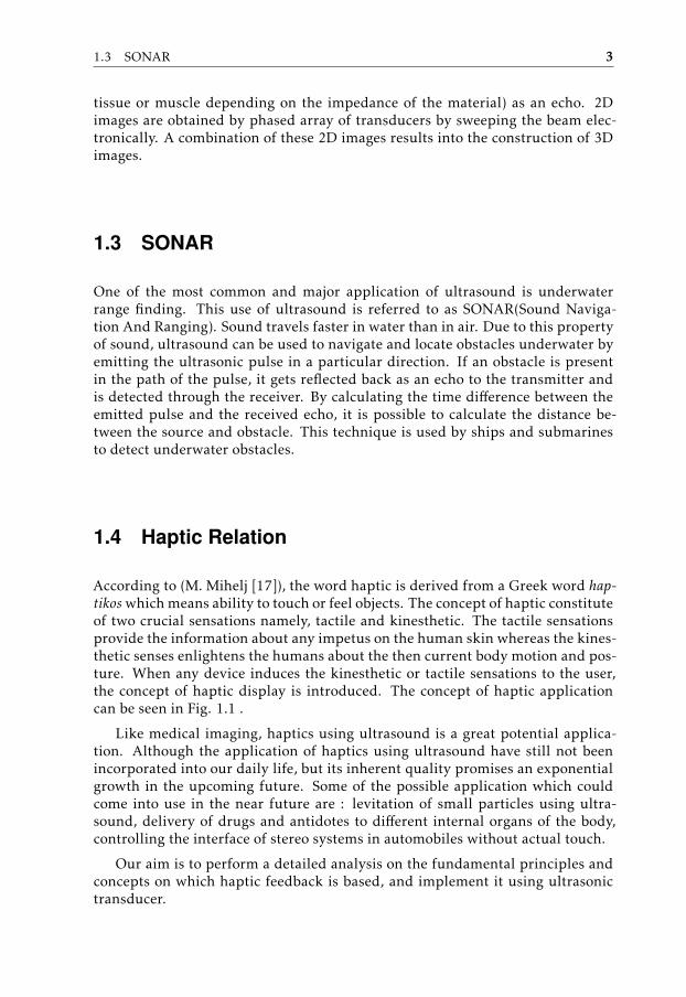
According to (M. Mihelj [17]), the word haptic is derived from a Greek word hap-tikos which means ability to touch or feel objects. The concept of haptic constituteof two crucial sensations namely, tactile and kinesthetic. The tactile sensationsprovide the information about any impetus on the human skin whereas the kines-thetic senses enlightens the humans about the then current body motion and pos-ture. When any device induces the kinesthetic or tactile sensations to the user,the concept of haptic display is introduced. The concept of haptic applicationcan be seen in Fig. 1.1 .
Like medical imaging, haptics using ultrasound is a great potential applica-tion. Although the application of haptics using ultrasound have still not beenincorporated into our daily life, but its inherent quality promises an exponentialgrowth in the upcoming future. Some of the possible application which couldcome into use in the near future are : levitation of small particles using ultra-sound, delivery of drugs and antidotes to different internal organs of the body,controlling the interface of stereo systems in automobiles without actual touch.
Our aim is to perform a detailed analysis on the fundamental principles andconcepts on which haptic feedback is based, and implement it using ultrasonictransducer.
4 1 Introduction
Figure 1.1: Virtual Sphere Created By Focused Ultrasound. Adapted FromBenjamin Long [3]
1.5 Goal of the Thesis
The main goal of the thesis is to conduct a system study on the principles ofhaptic, implementing electronic beamformation using ultrasound and creating asense of touch by constantly varying the acoustic pressure at the target point.
This is currently an upcoming research field and has tremendous potentialfor creating technical advancements in medical field. Since this field is still in itsnascent stage, no particular software or tool available for accurate modeling andaccurate validation of haptics. In order to accomplish the main goal of the thesisthe following tasks needs to be completed:
1. Studying the characteristics and transfer function of a piezoelectric trans-ducer to establish the mathematical relation between the frequency of theinput signal of the transducer and its corresponding output.
2. Understanding the principles underlying haptics.
3. Performing simulations on various characteristics of transducers using FieldII software.
4. Implementing the concept of phase delay to focus ultrasound beam at thetarget point.
5. Achieving a constant variation in pressure by using a pulse width modu-lated wave as input.
The credibility of this work depends on the implementation, application andthe evaluation methods.
2Theory
2.1 Basic of Ultrasonic Principles
Human ear is capable of perceiving sounds whose frequencies lie between 20Hzto 20 KHz. Any sound with the frequency greater than 20 KHz is termed as ultra-sound. The frequency of ultrasound is the number of cycles in one second and isinverse of the time period. According to (NDT [18]), the velocity of ultrasound isrelated to its wavelength as in Eq. (2.1)
λ =cf
(2.1)
where ’c’ is the velocity of ultrasound, ’f’ is the frequency of ultrasound and ’λ’ isits wavelength.
The waves representing ultrasound are either longitudinal(the particles mo-tion is along the line of propagation) or shear waves(the particle motion is per-pendicular to propagation direction). Ultrasound can be used to obtain informa-tion about an object. One such example is to calculate thickness of an object,according to (NDT [18]) is given by Eq. (2.2)
T =ct2
(2.2)
where ’T’ is the thickness of material, ’c’ is sound velocity, ’t’ is the time of flight.Every ultrasonic system has the potential to detect an errors in any obstacle
along its path of propagation. This property is described as sensitivity.
2.2 Piezoelectric Transducer
As per (Center [6]), a transducer is a simple device which converts one form of en-ergy to another form of energy. At the elementary level, a transducer is classified
5
6 2 Theory
into two categories namely input and output transducers. They differ with eachother on the basis of the type of input signal given to them. The transducers thatconvert electrical energy into another forms of energy, or vice versa with the useof material such as quartz crystal, are termed as piezoelectric transducers. Thisconversion of energy into various different forms inside piezoelectric transducersforms the base for ultrasound testing. When mechanical stress is applied to cer-tain piezoelectric material, they produce an electrical charge in response to thatinput. This process is termed as piezoelectric effect. The piezoelectric transducerproduces ultrasound when it is subjected to an electrical signal of a particularfrequency, thus acting as a transmitter. It can also produce electrical signal asan output when subjected to ultrasound, thus acting as a receiver. PiezoelectricTransducers are also classified based on their application : contact transducersand non contact transducers.
2.2.1 Contact Transducers
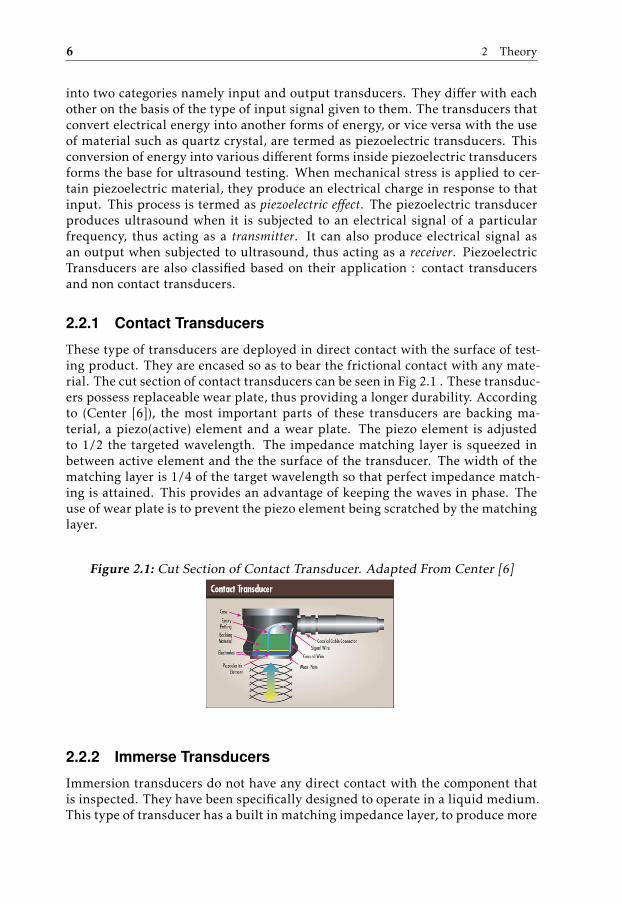
These type of transducers are deployed in direct contact with the surface of test-ing product. They are encased so as to bear the frictional contact with any mate-rial. The cut section of contact transducers can be seen in Fig 2.1 . These transduc-ers possess replaceable wear plate, thus providing a longer durability. Accordingto (Center [6]), the most important parts of these transducers are backing ma-terial, a piezo(active) element and a wear plate. The piezo element is adjustedto 1/2 the targeted wavelength. The impedance matching layer is squeezed inbetween active element and the the surface of the transducer. The width of thematching layer is 1/4 of the target wavelength so that perfect impedance match-ing is attained. This provides an advantage of keeping the waves in phase. Theuse of wear plate is to prevent the piezo element being scratched by the matchinglayer.
Figure 2.1: Cut Section of Contact Transducer. Adapted From Center [6]
2.2.2 Immerse Transducers
Immersion transducers do not have any direct contact with the component thatis inspected. They have been specifically designed to operate in a liquid medium.This type of transducer has a built in matching impedance layer, to produce more

2.3 Characteristics of Piezoelectric Transducers 7
sound energy in the liquid medium to inspect the component. It can be used in awater tank or bubbler system in scanning applications.
2.3 Characteristics of Piezoelectric Transducers
According to (Center [6]), the characteristics of piezoelectric transducers such asefficiency, resonance and damping are described briefly in this section.
2.3.1 Efficiency and Bandwidth
Efficiency of a transducer depends on its sensitivity and resolution. Sensitivityis directly proportional to the product of the both transmitter and receivers ef-ficiency. The capacity of a transducer to detect any errors near the surface ofmaterial is termed as resolution.
Every transducer has a frequency mentioned on it. This frequency is known asthe center frequency and is dependent on the backing material. The most efficientdamping is produced when the impedance of backing material is analogous tothat of the piezo element. The bandwidth and sensitivity of the transducers isdirectly proportional to the impedance matching. Bandwidth of transducers isinversely proportional to penetration of ultrasound in a material.
2.3.2 Resonance
Every transducer has a tendency to vibrate at its natural frequency with maxi-mum amplitude at its lowest harmonic frequency. The natural frequency of atransducer is dependent on its shape, size and material. Natural frequency isalso known as resonant frequency. When we provide an energy source possess-ing a frequency which is approximately equal to its natural frequency, the phe-nomenon known as resonance occurs. If the frequency of the energy source isgreater than the natural frequency, then the output frequency has a low ampli-tude.
2.3.3 Damping
The ability of a transducer to decrease the number of vibrations or noise is termedas damping. The process through which the system decreases the vibrations in-volves the absorption of some part of mechanical or electrical energy. One ad-vantage of damping phenomenon is that it helps alleviate the excess higher fre-quency unwanted noise.
2.3.4 Frequency Response
The transducer produces an output frequency in response to the frequency ofthe input given to it. This inherent property of the transducers to produce therequired frequencies is termed as frequency response.

8 2 Theory
2.4 RLC Model of a Piezoelectric Transducer
The RLC circuit of a piezoelectric device represents its electromechanical behav-ior.This model is valid for only one resonance. The RLC circuit can be seen in Fig2.2 . In the Fig 2.2, C0 is dielectric capacitance R1, C1, L1 are the resistor, capac-
Figure 2.2: RLC circuit of a piezoelectric device. Adapted From Asztalos [2]
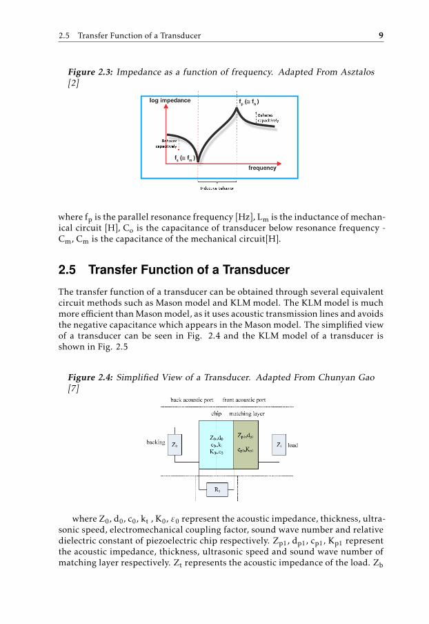
itor and inductor connected in series. According to (as in Asztalos [2] ), patternof piezo element’s response can be seen in Fig 2.3. It depicts that increase in cy-cling frequency is proportional to piezo’s first approximation of frequency wherethe impedance observed is minimal (fm) i e. at this point admittance is maximum.The fm is approximately equal to series resonance frequency, fs, where impedanceof piezo element is zero. With the further increase in cycling frequency, the risein impedance is maximum. The frequency at which this happens is symbolized asfn, which is approximately equal to the parallel resonance frequency fp. The max-imum impedance frequency is also termed as anti resonance frequency, fa. thepiezo element depicts capacitive behavior for frequencies f<fs and f>fp, whereasit depicts inductive behavior for frequency fm<f<fn.The maximum response fromthe piezo element is observed between fm and fn.
According to (Asztalos [2]), the series resonance frequency fs, is given by theEq. (2.3)
f s =1
2π
√1
L1C1(2.3)
where fs is the series resonance frequency [Hz], L1 is the inductance of mechani-cal circuit [H], and C1 is the capacitance of mechanical circuit [F]. According to(Asztalos [2] ), the parallel resonance frequency fp, is given by Eq. (2.4)
f p =1
2π
√Co + Cm
LmCoCm(2.4)
2.5 Transfer Function of a Transducer 9
Figure 2.3: Impedance as a function of frequency. Adapted From Asztalos[2]
where fp is the parallel resonance frequency [Hz], Lm is the inductance of mechan-ical circuit [H], Co is the capacitance of transducer below resonance frequency -Cm, Cm is the capacitance of the mechanical circuit[H].
2.5 Transfer Function of a Transducer
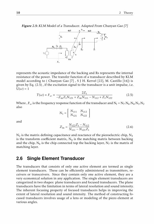
The transfer function of a transducer can be obtained through several equivalentcircuit methods such as Mason model and KLM model. The KLM model is muchmore efficient than Mason model, as it uses acoustic transmission lines and avoidsthe negative capacitance which appears in the Mason model. The simplified viewof a transducer can be seen in Fig. 2.4 and the KLM model of a transducer isshown in Fig. 2.5
Figure 2.4: Simplified View of a Transducer. Adapted From Chunyan Gao[7]
where Z0, d0, c0, kt , K0, ε0 represent the acoustic impedance, thickness, ultra-sonic speed, electromechanical coupling factor, sound wave number and relativedielectric constant of piezoelectric chip respectively. Zp1, dp1, cp1, Kp1 representthe acoustic impedance, thickness, ultrasonic speed and sound wave number ofmatching layer respectively. Zt represents the acoustic impedance of the load. Zb
10 2 Theory
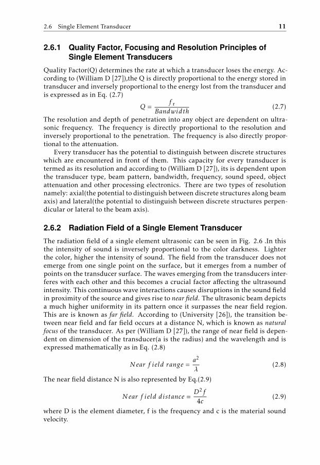
Figure 2.5: KLM Model of a Transducer. Adapted From Chunyan Gao [7]
represents the acoustic impedance of the backing and Rs represents the internalresistance of the power. The transfer function of a transducer described by KLMmodel according to ( Chunyan Gao [7] , S J H. Kervel [22], M. Castillo [16]) isgiven by Eq. (2.5) , if the excitation signal to the transducer is a unit impulse, i.e.U(ω) = 1
T (ω) = Fω =2Zt
−Z inZtN t21 + Z inN t11 − N t12 + ZtN t22(2.5)
Where , Fω is the frequency response function of the transducer and Nt = N7.N6.N4.N3.N2also
N t =[N t11 N t12N t21 N t22
]and
Z in =N t22Zt − N t12
N t11 − N t21Zt(2.6)
N2 is the matrix defining capacitance and reactance of the piezoelectric chip, N3is the transform coefficient matrix, N4 is the matching matrix between backingand the chip, N6 is the chip connected top the backing layer, N7 is the matrix ofmatching layer.
2.6 Single Element Transducer
The transducers that consists of only one active element are termed as singleelement transducers. These can be efficiently administered as transmitters, re-ceivers or transceivers. Since they contain only one active element, they are avery economical solution in any application. The single element transducers arecategorized in two shapes: plane transducers and focused transducers. The planetransducers have the limitation in terms of lateral resolution and sound intensity.The inherent focusing property of focused transducers helps in improving theextent of lateral resolution and sound intensity. The method of constructing fo-cused transducers involves usage of a lens or modeling of the piezo element atvarious angles.
2.6 Single Element Transducer 11
2.6.1 Quality Factor, Focusing and Resolution Principles ofSingle Element Transducers
Quality Factor(Q) determines the rate at which a transducer loses the energy. Ac-cording to (William D [27]),the Q is directly proportional to the energy stored intransducer and inversely proportional to the energy lost from the transducer andis expressed as in Eq. (2.7)
Q =f r
Bandwidth(2.7)
The resolution and depth of penetration into any object are dependent on ultra-sonic frequency. The frequency is directly proportional to the resolution andinversely proportional to the penetration. The frequency is also directly propor-tional to the attenuation.
Every transducer has the potential to distinguish between discrete structureswhich are encountered in front of them. This capacity for every transducer istermed as its resolution and according to (William D [27]), its is dependent uponthe transducer type, beam pattern, bandwidth, frequency, sound speed, objectattenuation and other processing electronics. There are two types of resolutionnamely: axial(the potential to distinguish between discrete structures along beamaxis) and lateral(the potential to distinguish between discrete structures perpen-dicular or lateral to the beam axis).
2.6.2 Radiation Field of a Single Element Transducer
The radiation field of a single element ultrasonic can be seen in Fig. 2.6 .In thisthe intensity of sound is inversely proportional to the color darkness. Lighterthe color, higher the intensity of sound. The field from the transducer does notemerge from one single point on the surface, but it emerges from a number ofpoints on the transducer surface. The waves emerging from the transducers inter-feres with each other and this becomes a crucial factor affecting the ultrasoundintensity. This continuous wave interactions causes disruptions in the sound fieldin proximity of the source and gives rise to near field. The ultrasonic beam depictsa much higher uniformity in its pattern once it surpasses the near field region.This are is known as far field. According to (University [26]), the transition be-tween near field and far field occurs at a distance N, which is known as naturalfocus of the transducer. As per (William D [27]), the range of near field is depen-dent on dimension of the transducer(a is the radius) and the wavelength and isexpressed mathematically as in Eq. (2.8)
Near f ield range =a2
λ(2.8)
The near field distance N is also represented by Eq.(2.9)
Near f ield distance =D2f
4c(2.9)
where D is the element diameter, f is the frequency and c is the material soundvelocity.
12 2 Theory
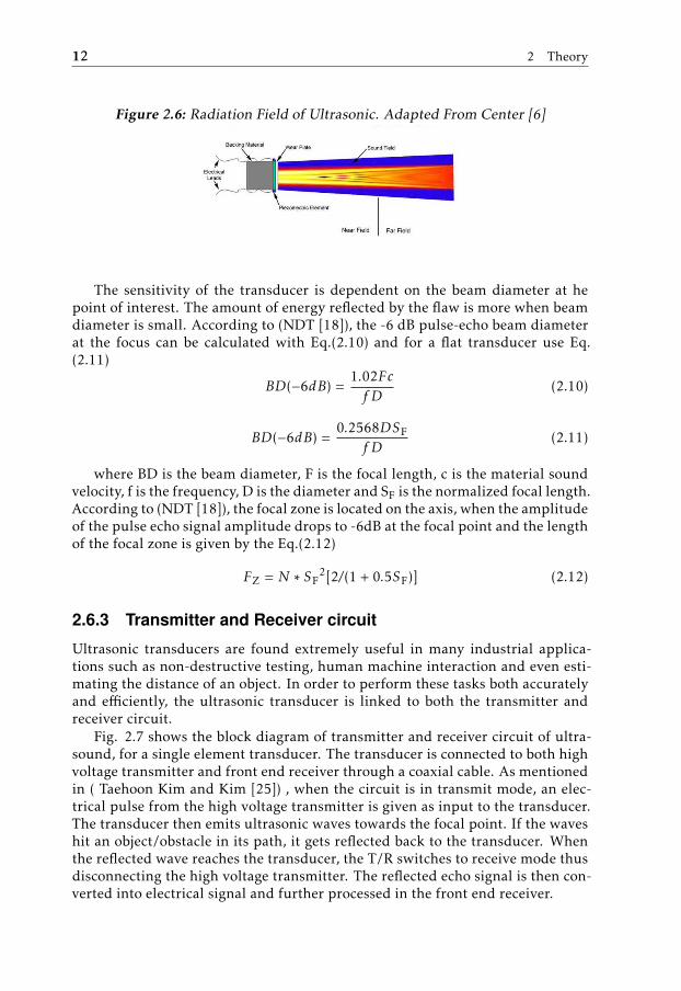
Figure 2.6: Radiation Field of Ultrasonic. Adapted From Center [6]
The sensitivity of the transducer is dependent on the beam diameter at hepoint of interest. The amount of energy reflected by the flaw is more when beamdiameter is small. According to (NDT [18]), the -6 dB pulse-echo beam diameterat the focus can be calculated with Eq.(2.10) and for a flat transducer use Eq.(2.11)
BD(−6dB) =1.02Fcf D
(2.10)
BD(−6dB) =0.2568DSF
f D(2.11)
where BD is the beam diameter, F is the focal length, c is the material soundvelocity, f is the frequency, D is the diameter and SF is the normalized focal length.According to (NDT [18]), the focal zone is located on the axis, when the amplitudeof the pulse echo signal amplitude drops to -6dB at the focal point and the lengthof the focal zone is given by the Eq.(2.12)
FZ = N ∗ SF2[2/(1 + 0.5SF)] (2.12)
2.6.3 Transmitter and Receiver circuit
Ultrasonic transducers are found extremely useful in many industrial applica-tions such as non-destructive testing, human machine interaction and even esti-mating the distance of an object. In order to perform these tasks both accuratelyand efficiently, the ultrasonic transducer is linked to both the transmitter andreceiver circuit.
Fig. 2.7 shows the block diagram of transmitter and receiver circuit of ultra-sound, for a single element transducer. The transducer is connected to both highvoltage transmitter and front end receiver through a coaxial cable. As mentionedin ( Taehoon Kim and Kim [25]) , when the circuit is in transmit mode, an elec-trical pulse from the high voltage transmitter is given as input to the transducer.The transducer then emits ultrasonic waves towards the focal point. If the waveshit an object/obstacle in its path, it gets reflected back to the transducer. Whenthe reflected wave reaches the transducer, the T/R switches to receive mode thusdisconnecting the high voltage transmitter. The reflected echo signal is then con-verted into electrical signal and further processed in the front end receiver.
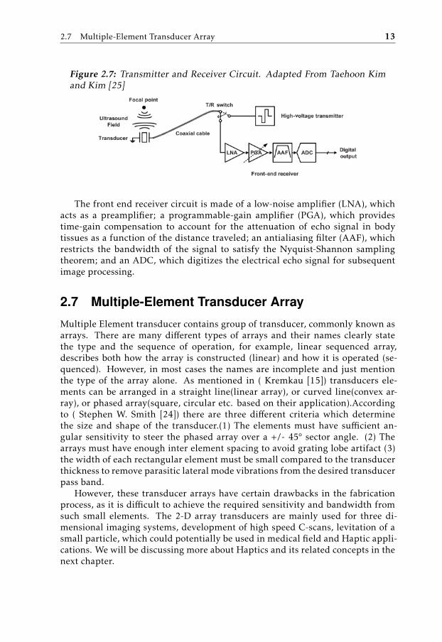
2.7 Multiple-Element Transducer Array 13
Figure 2.7: Transmitter and Receiver Circuit. Adapted From Taehoon Kimand Kim [25]
The front end receiver circuit is made of a low-noise amplifier (LNA), whichacts as a preamplifier; a programmable-gain amplifier (PGA), which providestime-gain compensation to account for the attenuation of echo signal in bodytissues as a function of the distance traveled; an antialiasing filter (AAF), whichrestricts the bandwidth of the signal to satisfy the Nyquist-Shannon samplingtheorem; and an ADC, which digitizes the electrical echo signal for subsequentimage processing.
2.7 Multiple-Element Transducer Array
Multiple Element transducer contains group of transducer, commonly known asarrays. There are many different types of arrays and their names clearly statethe type and the sequence of operation, for example, linear sequenced array,describes both how the array is constructed (linear) and how it is operated (se-quenced). However, in most cases the names are incomplete and just mentionthe type of the array alone. As mentioned in ( Kremkau [15]) transducers ele-ments can be arranged in a straight line(linear array), or curved line(convex ar-ray), or phased array(square, circular etc. based on their application).Accordingto ( Stephen W. Smith [24]) there are three different criteria which determinethe size and shape of the transducer.(1) The elements must have sufficient an-gular sensitivity to steer the phased array over a +/- 45° sector angle. (2) Thearrays must have enough inter element spacing to avoid grating lobe artifact (3)the width of each rectangular element must be small compared to the transducerthickness to remove parasitic lateral mode vibrations from the desired transducerpass band.
However, these transducer arrays have certain drawbacks in the fabricationprocess, as it is difficult to achieve the required sensitivity and bandwidth fromsuch small elements. The 2-D array transducers are mainly used for three di-mensional imaging systems, development of high speed C-scans, levitation of asmall particle, which could potentially be used in medical field and Haptic appli-cations. We will be discussing more about Haptics and its related concepts in thenext chapter.

3Haptic Research
3.1 Basics about Haptics
For haptics, an artificial ambiance is created where virtual objects are generatedthrough the means of some processing unit and then humans interact with thesevirtual objects through the means of motor sensations. Generally, any hapticbased unit comprises of a display, which depicts images and sound on the basisof human interaction with the computer. The generation of any virtual objector of the haptic sensations is dependent on human’s capability to decipher theobjects haptic parameters, the technical ability to generate objects in real timeand the precision of haptic device for providing the right stimulus.
Any haptic system that constitute only visual and audio sensations of the userlimits its application. However the haptic system that involves the audio-visualsensations and most importantly comprises of providing the opportunity to hu-mans for manipulating the objects such as grasping, moving, etc is considered tobe a highly efficient haptic unit.
According to (M. Mihelj [17]), a haptic interface is the device that is used formanipulation of virtual objects. It records positions/impetus force and displaysthe same after manipulation, to the user. This device acts as a substitute for handrelated tasks in real world. It receives motor inputs from the user and in responseto that, it displays haptic image to the user.
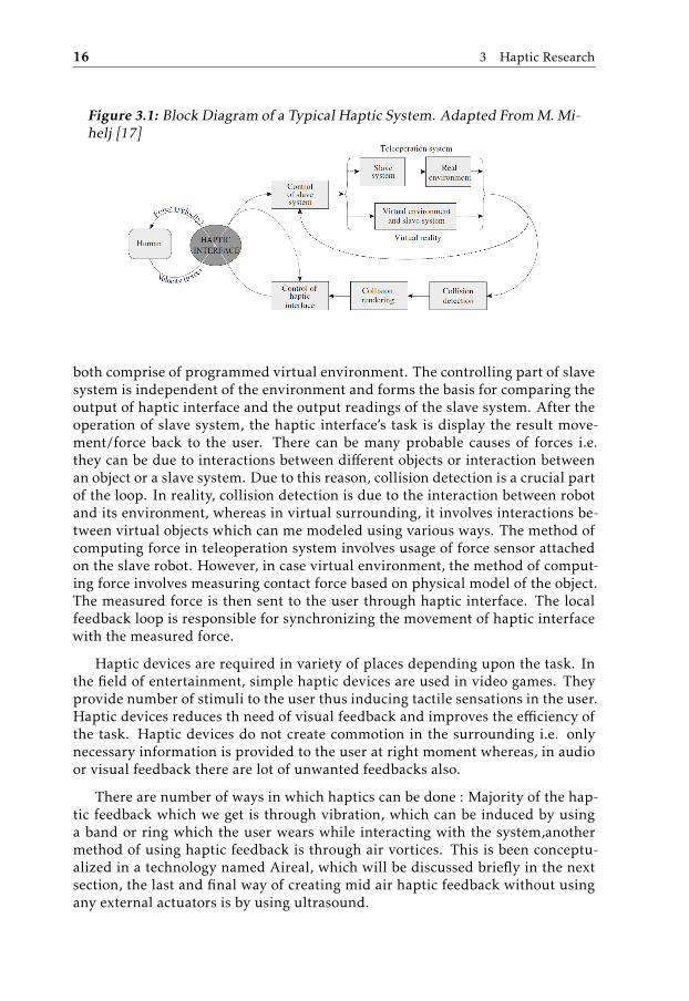
According to (M. Mihelj [17]), the typical block diagram of any haptic sys-tem can be seen in Fig. 3.1 The human interacts with the haptic interface viathe means of any movement. This interface gauges and records the stimulus pro-vided by the human. The recored input value is used as a reference input tothe teleoperation system or to the virtual environment. The teleoperation systemconsists of a slave robot, whose job is to perform the task in reality, that the hu-man instructs to the interface. The slave system and the object affected by it ,
15
16 3 Haptic Research
Figure 3.1: Block Diagram of a Typical Haptic System. Adapted From M. Mi-helj [17]
both comprise of programmed virtual environment. The controlling part of slavesystem is independent of the environment and forms the basis for comparing theoutput of haptic interface and the output readings of the slave system. After theoperation of slave system, the haptic interface’s task is display the result move-ment/force back to the user. There can be many probable causes of forces i.e.they can be due to interactions between different objects or interaction betweenan object or a slave system. Due to this reason, collision detection is a crucial partof the loop. In reality, collision detection is due to the interaction between robotand its environment, whereas in virtual surrounding, it involves interactions be-tween virtual objects which can me modeled using various ways. The method ofcomputing force in teleoperation system involves usage of force sensor attachedon the slave robot. However, in case virtual environment, the method of comput-ing force involves measuring contact force based on physical model of the object.The measured force is then sent to the user through haptic interface. The localfeedback loop is responsible for synchronizing the movement of haptic interfacewith the measured force.
Haptic devices are required in variety of places depending upon the task. Inthe field of entertainment, simple haptic devices are used in video games. Theyprovide number of stimuli to the user thus inducing tactile sensations in the user.Haptic devices reduces th need of visual feedback and improves the efficiency ofthe task. Haptic devices do not create commotion in the surrounding i.e. onlynecessary information is provided to the user at right moment whereas, in audioor visual feedback there are lot of unwanted feedbacks also.
There are number of ways in which haptics can be done : Majority of the hap-tic feedback which we get is through vibration, which can be induced by usinga band or ring which the user wears while interacting with the system,anothermethod of using haptic feedback is through air vortices. This is been conceptu-alized in a technology named Aireal, which will be discussed briefly in the nextsection, the last and final way of creating mid air haptic feedback without usingany external actuators is by using ultrasound.

3.2 Haptics using Air Vortices 17
3.2 Haptics using Air Vortices
AIREAL is a technology that produces tactile sensations in the air without the useof any equipments to be worn while experiencing it. It is a huge boost in this fieldas not wearing any physical equipments will not hamper natural user interaction.The concept described in this paragraph about AIREAL is derived from (Rajin-der Sodhi [21]). AIREAL induces tactile sensation in mechanoreceptors by theuse of air pressure fields , which are compressed in nature. It involves the usageof air vortices to impart the haptic feel . Air vortices are the rings of air, whichinduce a force that the user feels while interacting with it. An air vortex is formedwhen air is squeezed out of a circular opening. The air particles at the center ofthe opening moves with a higher speed as compared to the particles which arepresent at the edges of the ring. This difference in speed is due to the frictionalpull between particles of air. When the air ejects from the opening, the speedanomalies between different molecules results into the circular formation of airin the form of a ring. As this ring increases its diameter and passes a nominalvalue, it kicks off from the opening of AIREAL and travels through the air by us-ing its rotatory momentum. This rotatory motion inhibits the amount of energyloss and hence helps in maintaining the stability of vortex. The advantages ofusing these air vortices are: Tactile sensations can be felt over large distances, theequipment for generation of vortices in comparatively cheap and the air vorticescan be dynamically directed to a particular location by controlling the configu-ration of the nozzle in AIREAL . According to (Rajinder Sodhi [21]), air vorticesare described as a field where behavior of air has been noticed in a whirlpoolmotion circumventing a translational axis. The air vortices exert a considerableamount of force when they collide any obstacle in their field of propagation andcan traverse upto long distances without getting degraded in speed and form. AnAIREAL device trasnmitting air vortex can be seen in Fig. 3.2
3.3 Haptics using Ultrasound
Haptic touch generation using ultrasound is one of the most interesting tech-nique. In this approach we use the principle of acoustic radiation pressure byfocusing ultrasound. The ultrasonic transducers emit Ultrasound which is madeto converge and create a primary focal point by the concept of beamforming andphase computation. (Beamforming will be discussed in detail later in this chap-ter). This acoustic force when reflected from the focal point, creates a displace-ment in the skin tissue, which in turn induces a feeling of touch in the mechanore-ceptors of our skin. However a single ultrasonic transducer doesn’t have enoughpotential to create the force required to activate the mechanoreceptors in the skin.As a result, an array of transducers is needed to create required force to create asense of touch and this force can be varied by changing the size of the array oftransducers. By this approach, we can create the feel of 3 dimensional shapes inmid air without any external actuators. Biologically, the mechanoreceptors aredensely populated at the fingertips as compared to the palm. This is the reason

18 3 Haptic Research
Figure 3.2: AIREAL device ejecting air vortex that can be felt on hand.Adapted From Rajinder Sodhi [21]
why the haptic feedback is more strong at our fingertips as compared to rest of thepalm. One factor which makes ultrasound better when compared to other tech-niques is its increased accuracy and the range at which the tactile sensation canbe felt. By the use of ultrasonic transducer array, a single feedback point couldbe formed at finger to provide a feel of mid air haptics. Later, this single pointof feedback can be altered in position continuously so as to provide an illusion ofcontinuous movement at human hand.
3.4 Principles used in Haptics
Acoustic waves are longitudinal in nature and inherit the concept of reflection,interference and diffraction. According to (Beyer [4]) the wave equation is repre-sented by Eq.(3.1)
δ2p
δx2 −1c2δ2p
δt2= 0 (3.1)
where ’p’ is the acoustic pressure and ’c’ is the speed of sound and ’x’ is itsposition.
3.4.1 Acoustic Radiation Force
Whenever an acoustic wave strikes any object along its line of propagation, itresults into the creation of a force, which is then exerted on that inhibiting ob-ject. This force is termed as acoustic radiation force. This force is represented bynegative gradient of Gor’kov potential in Eq.(3.2). We can understand the mainmechanism underlying the acoustic radiation force by using a simple analysis.

3.4 Principles used in Haptics 19
We assume that the particle is spherical and rigid with dimensions smaller thanthe wavelength of the incident wave, but much larger than the viscous and ther-mal skin depth. By looking into this idea, we realize that no force will appear onthe particle if it has the same acoustic properties as the surrounding medium.Thefactors which govern acoustic radiation force are size of particle, amplitude of ul-trasound and acoustic contrast. Hence, the field incident on the particle will bereflected from its surface.
As a result, the radiation force acting on the particle will be a combination ofthe incident and reflected wave. According to(Asier Marzo and Drinkwater [1])to calculate the force exerted on a sphere due to a complex pressure field, thenegative gradient of the Gor’kov potential U is used as in (3.2)
F = − 5U (3.2)
and the complex acoustic pressure P at point r due to a piston source emitting ata single frequency is shown in Eq. (3.3)
P (r) = P 0ADf(θ)d
exp i(φ + kd) (3.3)
where P0 represents transducer amplitude and is a constant, A is the peak to peakamplitude of the excitation signal, d is the propagation distance in free space. Dfis the far- field directivity function, which depends on the angle between thetransducer normal and r. Directivity is the measure of degree to which the soundemitted from a source is concentrated in a particular direction. The directivityfunction of a circular piston source as in (Asier Marzo and Drinkwater [1]) isrepresented by Eq. (3.4)
Df = 2J1(kasinθ)/kasinθ (3.4)
where J1 is the Bessel function, a is the piston radius, k is the wave number, andis given as k = 2π/λ, where λ is the wavelength and φ is the initial phase of thepiston. The directivity plot of a transducer is shown in Fig. 3.3.
Figure 3.3: A typical directivity plot of transducer. Adapted From Park [19]
As per, (Asier Marzo and Drinkwater [1]), the potential function is expressedusing the acoustic pressure and velocity as shown in Eq.(3.5).
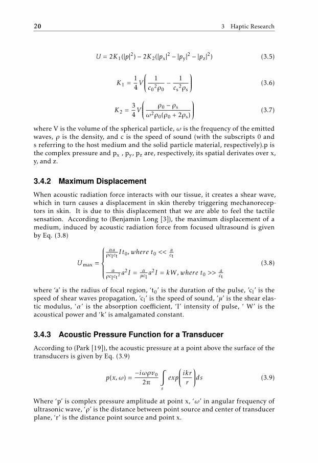
20 3 Haptic Research
U = 2K1(|p|2) − 2K2(|px|2 − |py|2 − |pz|2) (3.5)
K1 =14V
1c0
2ρ0− 1cs
2ρs
(3.6)
K2 =34V
ρ0 − ρs
ω2ρ0(ρ0 + 2ρs)
(3.7)
where V is the volume of the spherical particle, ω is the frequency of the emittedwaves, ρ is the density, and c is the speed of sound (with the subscripts 0 ands referring to the host medium and the solid particle material, respectively).p isthe complex pressure and px , py, pz are, respectively, its spatial derivates over x,y, and z.
3.4.2 Maximum Displacement
When acoustic radiation force interacts with our tissue, it creates a shear wave,which in turn causes a displacement in skin thereby triggering mechanorecep-tors in skin. It is due to this displacement that we are able to feel the tactilesensation. According to (Benjamin Long [3]), the maximum displacement of amedium, induced by acoustic radiation force from focused ultrasound is givenby Eq. (3.8)
Umax =
αaρclct
I t0, where t0 <<act
αρclct
2 a2I = α
µcla2I = kW , where t0 >>
act
(3.8)
where ‘a’ is the radius of focal region, ‘t0’ is the duration of the pulse, ’cl’ is thespeed of shear waves propagation, ’cl’ is the speed of sound, ’µ’ is the shear elas-tic modulus, ‘α’ is the absorption coefficient, ‘I’ intensity of pulse, ‘ W’ is theacoustical power and ‘k’ is amalgamated constant.
3.4.3 Acoustic Pressure Function for a Transducer
According to (Park [19]), the acoustic pressure at a point above the surface of thetransducers is given by Eq. (3.9)
p(x, ω) =−iωρv0
2π
∫s
exp
ikrrds (3.9)
Where ‘p’ is complex pressure amplitude at point x, ‘ω’ in angular frequency ofultrasonic wave, ‘ρ’ is the distance between point source and center of transducerplane, ‘r’ is the distance point source and point x.
3.5 Beamforming 21
For Far Field
For far field, the complex pressure is divided into two parts: on axis and off axis.The on axis pressure decays exponentially with the increase in distance from thesimulation plane as described in (Park [19]) is given by Eq. (3.10)
p(z, ω) = ρcv0
exp(ikz) − exp(ik2√z2 − a2)
(3.10)
Where ‘z’ is the distance between on axis point and transducer surface, ‘a’ is theradius of the transducer, ‘ρ’ is the distance between the point source and centerof transducer plane, ‘k’ is the wave-number, ‘c’ is the speed of sound, ‘v0’ is theconstant velocity of sound in z direction.
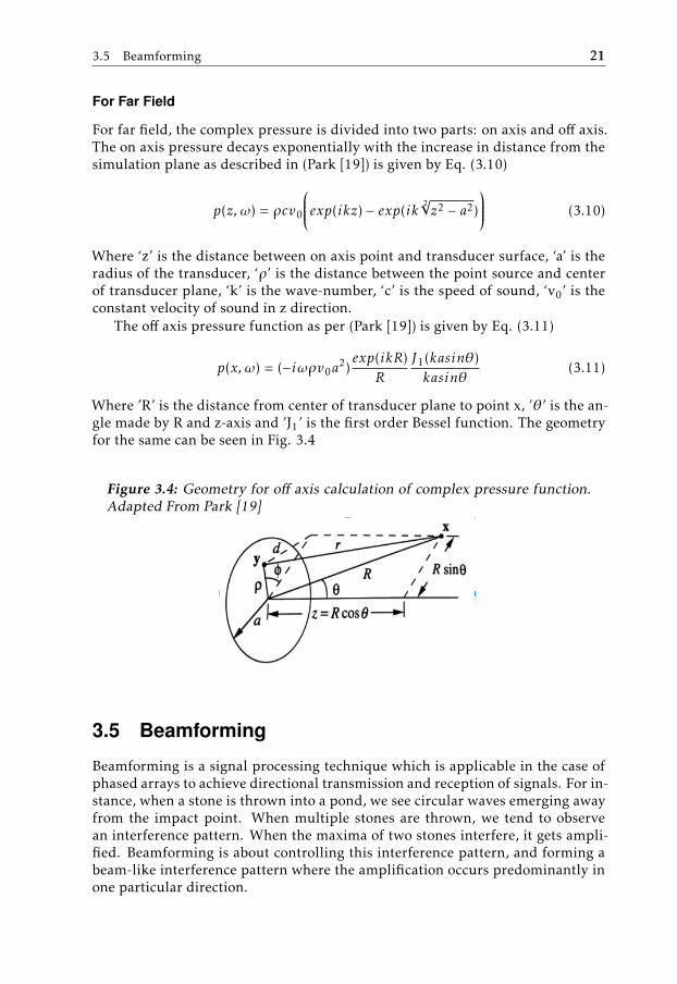
The off axis pressure function as per (Park [19]) is given by Eq. (3.11)
p(x, ω) = (−iωρv0a2)exp(ikR)
R
J1(kasinθ)kasinθ
(3.11)
Where ’R’ is the distance from center of transducer plane to point x, ’θ’ is the an-gle made by R and z-axis and ’J1’ is the first order Bessel function. The geometryfor the same can be seen in Fig. 3.4
Figure 3.4: Geometry for off axis calculation of complex pressure function.Adapted From Park [19]
3.5 Beamforming
Beamforming is a signal processing technique which is applicable in the case ofphased arrays to achieve directional transmission and reception of signals. For in-stance, when a stone is thrown into a pond, we see circular waves emerging awayfrom the impact point. When multiple stones are thrown, we tend to observean interference pattern. When the maxima of two stones interfere, it gets ampli-fied. Beamforming is about controlling this interference pattern, and forming abeam-like interference pattern where the amplification occurs predominantly inone particular direction.

22 3 Haptic Research
In our case, we use small piezoelectric transducers instead of stones to createthe interference pattern. As mentioned in the previous chapter, when an alter-nating voltage signal is applied to the piezoelectric transducer, it starts to vibrateand emits sound. If the spacing between the transducer elements and the delay inthe element’s signals is just right, we can create an interference pattern accordingto our needs, where in majority of the signal energy is focused in one angular di-rection. The same principle is applied when the transducer is used to receive thesound. Just by adjusting the amplitude and delay of the received signal on eachtransducer element, it is possible to receive the echo from a particular angulardirection. According to (Biegert and 2018 [5]), beamforming can be formulatedmathematically using Eq. (3.12)
ζ(θ) =k=N∑k=0
ak(θ).xk (3.12)
where N is the number of elements, k is the index variable, ak is the complexcoeffecient of the kth element, xk is the voltage response from the kth element, ζis the beam response, θ is the angle of the beam main lobe.
3.5.1 Analog Beamforming
In this beamforming, the input analog signal at the transmitter is altered dueto the modifications in amplitude or phase. After transmission, the signals areadded before ADC conversion at receiver. A traditional analog filter comprises oftransducer array for transmission and receiving of signals and analog filter for thepurpose of filtration of the received signal. This analog filter consists of a delayline. The role of this delay line is to add delay to each of the received signal. thetwo advantages of using analog filter in an ultrasound system is that it reducesthe power consumption of the system and decreases the number of componentsin system. Analog beamforming can be performed in variety of ways in differentimplementation setups.
• When pressure waves are the signals at the receiver and transducer arrayconvert these signals to voltage or current.
• When different types of filter such as narrow filter, finite impulse responsefilter or infinite impulse response filter are used in the analog filter sectionbefore the receiver.
• Two types of modules can be used for reducing the side lobes ; either sum-mation module or apodization circuit.
The typical transmitter and receiver module displaying analog beamforming canbe seen in Fig. 3.5 and Fig. 3.6
3.5.2 Digital Beamforming
In digital beamforming, the amplitude and phase modifications are made to thedigital signal before the Digital to analog converter in transmission side. In

3.5 Beamforming 23
Figure 3.5: Analog Beamforming Transmitter. Adapted From World [28]
Figure 3.6: Analog Beamforming Receiver. Adapted From World [28]
the receiving end each transducer element is connected to an analog to digitalconverter(ADC) followed by the signal summation.The block diagram of digitalbeamforming is shown in Fig.3.7.
Figure 3.7: Transmitter and Receiver of Digital Beamformer. Adapted fromKerem Karadayi and Kim [13]

24 3 Haptic Research
Once, the received signal passes through analog signal conditioning, the sig-nals are digitized using ADCs, so that digital beamforming can be performed.After beamformation, the signal goes into demodulator, to get rid of the carrierfrequency of and extract the complex baseband data. This data is then used forsignal and image processing.
Figure 3.8: Schematic diagram illustrating the principle of digital beam-forming. Adapted from Kerem Karadayi and Kim [13]
Figure 3.8 is a schematic diagram showing the principle of digital beamform-ing. Each transducer element receive the reflected echo signal from the targetpoint at different timings. According to (Kerem Karadayi and Kim [13]) in Fig.3.8 the element in the center receives the signal first when compared to otherelements. The transducers at both the ends will be the last to receive the echo.The received echoes are then aligned properly by introducing appropriate delayto each channel, before summation.
Time delay quantization errors are minimized in digital beamforming. Thedelay accuracy in analog beamformers is in the range of 20ns. For operationsat high frequencies (above 10MHz) the quantization noise will appear due tothe increase in the side lobe level, thus reducing the contrast resolution. Thedigital beamformers can be used in high frequency operations due to its greatlyimproved delay accuracy.
3.6 Computation of Amplitude and Phase
In this section we discuss the computation of phase and amplitude at differentcontrol points. To get haptic feedback, amplitude at each control point needsto be controlled. We can do this by changing the phase to make the waves con-structively interfere in points of high amplitude and destructively interfere inpoints of low amplitude. So, to obtain the desired amplitudes at the given points,we must determine the phase values relative to each other. According to (Ben-jamin Long [3]) , control points with same amplitude, tend to amplify each other
3.6 Computation of Amplitude and Phase 25
if they move closer and their phase difference is zero, or cancel out each other ifthe phase difference is half a period and they move closer.
3.6.1 Model of Acoustic Field
To understand the calculation of phase and amplitude, it is of paramount impor-tance to understand the acoustic field, ψ produced by n ultrasonic transducers.According to (Emad S. Ebbini [8]), the wavefunction at far field in 3D can bemathematically stated as in Eq. (3.13)
f (∆x,∆y,∆z) =eik 2
√(∆x)2 + (∆y)2 + (∆z)2
[((∆x)2 + (∆y)2 + (∆z)2)2]34
(3.13)
where ∆x = x-x’, ∆y = y-y’, ∆z = z-z’ and x, y, z are the coordinates with re-spect to the aperture and x’, y’, z’ provide absolute positions in far field. Thesound wave emitting from a transducer q can be divided into 4 parts: productof emission amplitude Aq
emit ,a phase offset eiφq , amplitude attenuation function
Aqattn(x′ , y′ , z′) and a phase difference function eikq(x′ ,y′ ,z′). So for n transducers,
the field ψΩ is expressed mathematically by Eq. (3.14)
ψΩ(x′ , y′ , z′) =n∑q=1
Aqemiteiφq .ψq(x′ , y′ , z′) (3.14)
where ψq(x′ , y′ , z′) is the product of Aqattn(x′ , y′ , z′) and eikq(x′ ,y′ ,z′). Now a set
of m control points were selected in x’, y’, z’ and are represented by (χ1,...χm),where each elements gives information about phase and amplitude and are com-ponent of field φΩ. The phase and amplitude can be obtained by equation Ax =b, where A is given by
A =
ψ1(χ1) . . . ψn(χ1)...
. . ....
ψ1(χm) . . . ψn(χm)
and vector x is given by [A1
emit eφ1 ,....,Anemit eφn ]T and b is given by [ψ′Ω(χ1),...ψ′Ω(χ1)]T
and these values are solved using the minimum solver algorithm as presented in(Emad S. Ebbini [8]).
3.6.2 Mathematical Representation of Phase and Amplitude
A matrix R is used to represent the phase and amplitude effect of one controlpoint on other. This is shown by the Eq. (3.15)
Rx = λx (3.15)
According to (Benjamin Long [3]) we can quite simply find a solution for any onecontrol point, we then use symbolic algebra to algebraically generate a simplified

26 3 Haptic Research
minimum-norm solution for each single control point case:
Aqemiteiφq =
Aqattn(χC − χq)eikq(χC−χq)AC∑n
i=0(Aiattn(χC − χi)2)
(3.16)
where χC is the position of the control point, with AC its amplitude, while χq isthe transducer origin. Using these resulting complex values for the transduceremissions from Eq. (3.14), we generate hypothesized single control point fieldsψΩ C
1,...,m. From this matrix R is constructed
R =
ψ1(χC1 ) . . . ψm(χC1 )
.... . .
...ψ1(χCm ) . . . ψm(χCm )
which is the vector of amplitude and phases of the control point depending onthe amplification eigenvalue given. The estimation of maximally amplified con-trol points is generated by the assumption of weighted ’mixing’ of each singlecontrol point solution. Therefore, finding a large eigenvalue λ leads to a largeconstructive amplification of phases in the eigenvector. This phase can then beused in any linear system to generate similar amplitudes and for more efficienttransducer usage. A simple power method can be used to find the eigenvectorwith the largest eigenvalue. This method can be estimated and restarted fromprevious solution, thus providing a time-bound solution. By using this method,it is possible to make control points of a linear system coexist, thus reducing theexclusion caused by destructive interference and noise by constructive interfer-ence.
3.6.3 Optimization of Calculated Parameters
Now that we calculated the phases and amplitude for the array of transducers, itsimportant that we set some algorithm to optimize the power and easily modifythe matrix configuration. For this, the algorithm called tikhonov regularizationwas used according to (Benjamin Long [3]). In this the the linear system Ax = bwas enlarged and modified as
Aσ1
γ . . . 0...
. . ....
0 . . . σnγ
x =
b0...0
and σq can be represented by Eq.
σq =
√√∣∣∣∣∣∣∣∣∣∣∣∣ m∑i=0
Aqattn(χCi − χq)ACi
m
∣∣∣∣∣∣∣∣∣∣∣∣ (3.17)
where γ is either 0 or 1 depending on whether the method for computing phaseand amplitude involves the usage of minimum norm solver algorithm or if it

3.7 Alternate Method Used for Amplitude Modulation 27
involves the optimization of amplitude to equal values so as to provide betterpower emission.
3.6.4 Haptic Efficiency
Once the computation of phase and amplitude is achieved, the next step is lowfrequency modulation. As described in (Asier Marzo and Drinkwater [1]), hapticsis only perceivable by humans at 200 Hz and to attain this 200 Hz modulation(Benjamin Long [3]), the array is is excited for (1/400)th second period and then isnot excited for next (1/400)th second period. However, as a result of this process,there is a considerable undesired loss in power.
So, a solution for outwitting this obstacle is achieved which involves usingof both the halves of modulation cycle to attribute for the output. It involvescareful generation and division of control points in two different parts and thenemitting them in an alternating manner. The proximity of the control pointsdetermines the effectiveness of phase computation method. So based on this,usage of principal component analysis provides with probability of bifurcatingthe plane into two highly populated control point groups. Therefore, by choosingbetween either of the fields in a continuous manner, a powerful perception oftactile sensations is created.
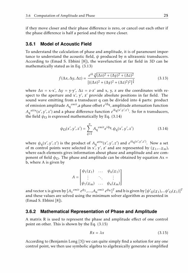
3.6.5 Summary of the Wave Synthesis Algorithm
The procedure for wave generations involves the following steps: The acosuticfield produced by a single transducer is being calculated and is then projected asa large modeled volume. Then that particular transducer undergoes offsetting forposition , phase and amplitude for real values. This involves formations of con-structive interferences and destructive interferences. After this a control point isdefied in the plane . Then optimal values of phase is calculated. There will bemore than one solutions(so there will be repeated calculations of the phases) foroptimal value of phases but the value with maximum intensity is being sent tothe transducer array. The flowchart for the same can be seen in Fig. 3.9
3.7 Alternate Method Used for Amplitude Modulation
The previous section describes the wave synthesis algorithm and amplitude com-putation in a generic way. Another way of implementing amplitude modulationof the input wave (for the purpose of achieving tactile sensation) is presented inthis section. It was adapted from (Peter R. Smith and Freear [20]).
The concept which was used in implementation of this thesis work was de-rived from the method presented in this section and will be discussed in theresults section of the thesis.
28 3 Haptic Research
Figure 3.9: Algorithm of Wave Synthesis
3.7.1 Input wave
The input wave given to the transducer can be of any type and in our case weuse a half square wave. Despite using a half square wave, we get a sinusoidaloutput from the transducer due to its resonating nature. In order to get the tactilesensation, the output wave from the transducer needs to be modulated at 200Hz
3.7 Alternate Method Used for Amplitude Modulation 29
frequency. So, for the transducer to emit a sound wave modulated at a particularfrequency, the input signal show be pulse width modulated.
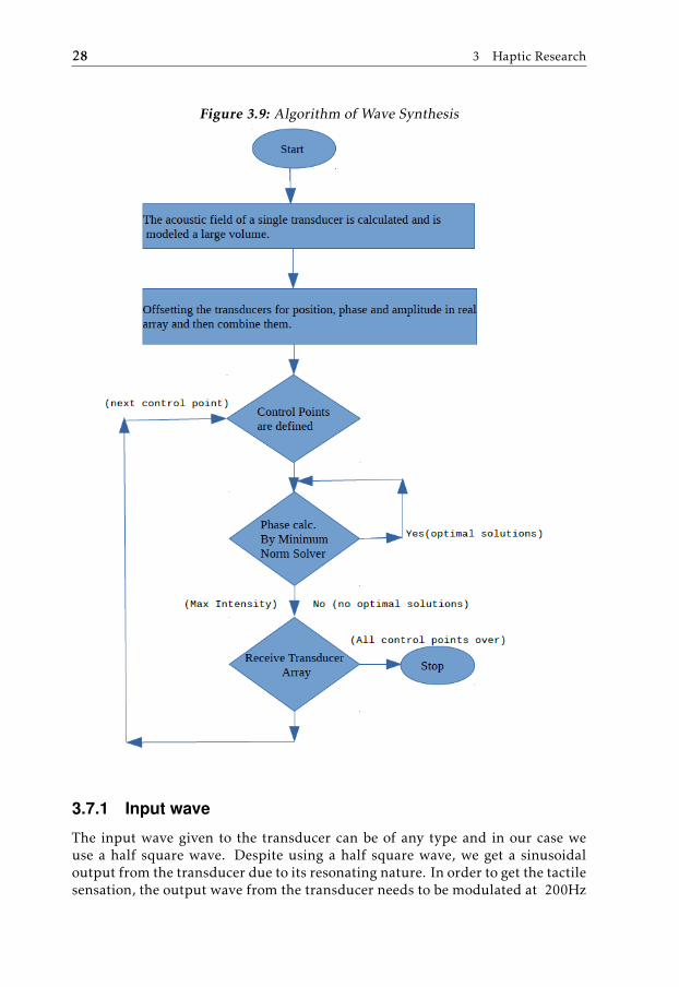
Figure 3.10: Triangular (sawtooth) symmetrical pulse width modulationconsisting of a carrier (dotted line), and a desired output level(gray solidline). Adapted From Peter R. Smith and Freear [20]
The conventional carrier based PWM generates pulses of varying width bycomparing the carrier wave of known form to a desired output level or modu-lating wave. As seen in Fig. 3.10 a conventional triangular carrier wave with aspecific output level can vary the pulse width of the output wave in a linear fash-ion. Therefore the width of the output pulse is directly proportional to the dclevel.
A linear triangular carrier wave is defined as
c(t) = A.|(2/π)(sin-1(sin(ωt + φ)))| + L (3.18)
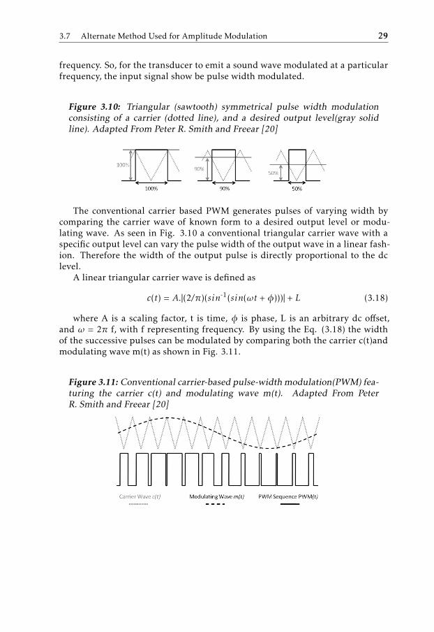
where A is a scaling factor, t is time, φ is phase, L is an arbitrary dc offset,and ω = 2π f, with f representing frequency. By using the Eq. (3.18) the widthof the successive pulses can be modulated by comparing both the carrier c(t)andmodulating wave m(t) as shown in Fig. 3.11.
Figure 3.11: Conventional carrier-based pulse-width modulation(PWM) fea-turing the carrier c(t) and modulating wave m(t). Adapted From PeterR. Smith and Freear [20]

4Implementation
This chapter describes the implementation of Matlab Based Graphical User In-terface (GUI) describing the various elements involved in ultrasonic transducerconfiguration simulation. It involves validation and modifications made in thisGUI, with the aim of incorporating the concept of haptics through it. After thatthe chapter describes the mathematical equation incorporated by us to imple-ment haptics and how it is different from the generic application of haptics. Thesecond part of this chapter describes the use of an ultrasonic transducer simu-lation platform named ’Field II’. This platform allowed us to develop varioustransducers configurations and plot its impulse responses in different scenarios.The third part of this chapter states concept developed by us though Matlab codeto represent the concepts of beamforming, transducer geometry, delay generationand phase generation for array of transducers.
31

32 4 Implementation
4.1 Matlab Based GUI
The Fig. 4.1 depicts the graphical user interface named as Transducer array Cal-culation(TAC), which was taken from (Kohout [14]). This simulation platformalleviates the need for any hardware tools required to run trials for computingvarious parameters of ultrasonic transducers. It helps us to visualize directivitypatterns, near field region, far field region of a transducer. It provides us with thepossibility to configure transducer array size, selection of single element in thearray, excitation of input signal and impedance and attenuation characteristicsof a transducer. It helps us to view the input signal either in time or frequencydomain, the relationship between angle of the transducer and its frequency, di-rectivity pattern of a transducer, pressure variation in near field. it provides auser friendly feature of importing user input configuration of transducers, atten-uation user input file, impedance user input file and user input excitation signal.
Figure 4.1: Original GUI. Adapted From Kohout [14]
4.1.1 Input Field
The input platform of the TAC GUI is shown in the Fig. 4.2 . The GUI allows theuser to load and save the transducer configuration, select the type of excitationsignal given to the transducer, change the transducer geometry, spacing betweenthe transducer and load attenuation and impedance configuration of the trans-ducer.
A new transducer configuration can be given by the user by changing thefollowing parameters like number of X and Y elements, spacing between the Xand Y elements, phase shift of the excitation signal in both X and Y direction,

4.1 Matlab Based GUI 33
Figure 4.2: Input Parameters of Transducer. Adapted From Kohout [14]
rectangular patch parameters of individual elements. In the transducer array,every single element can be configured separately. It is possible to activate anddeactivate individual elements using the green and red buttons as shown in Fig.4.3. A single element from the array can be selected and visualized to know thephase and amplitude of the element.
Figure 4.3: Single Element Configuration. Adapted From Kohout [14]
4.1.2 Excitation Signals
The excitation signal given to the transducer can also be selected and modifiedaccording to the user requirements. By clicking the ’options’ button present onthe right top of the array input parameters, the input wave can be selected as

34 4 Implementation
shown in Fig. 4.4. The frequency and other parameters can be set by the userto achieve the desired input waveform. It is also possible to load any arbitrarysignal by using the option’ other wave’. The input signal can be represented inboth time and frequency domain.
Figure 4.4: Excitation Signal Editor. Adapted From Kohout [14]
4.2 Modified GUI
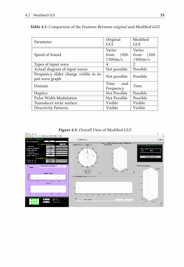
The modified version of GUI can be seen in Fig. 4.5. These modifications weredone by us by keeping in mind the following aim: adding and deleting featuresaccording to the requirements and specifications of our project. The inclusion ofadditional parts required the coding in Matlab. The Matlab codes for the updatedcomponents can be found in the Appendix section. The differences in originaland modified GUI are summarized in Table. 4.1
4.2 Modified GUI 35
Table 4.1: Comparison of the Features Between original and Modified GUI
ParameterOriginalGUI
ModifiedGUI
Speed of SoundVariesfrom (300-1500)m/s
Variesfrom (300-1500)m/s
Types of input wave 4 2Actual diagram of input waves Not possible PossibleFrequency slider change visible in in-put wave graph
Not possible Possible
DomainTime andFrequency
Time
Haptics Not Possible PossiblePulse Width Modulation Not Possible PossibleTransducer array surface Visible VisibleDirectivity Patterns Visible Visible
Figure 4.5: Overall View of Modified GUI
36 4 Implementation
4.3 Field II
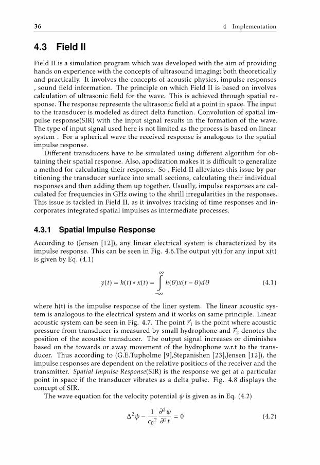
Field II is a simulation program which was developed with the aim of providinghands on experience with the concepts of ultrasound imaging; both theoreticallyand practically. It involves the concepts of acoustic physics, impulse responses, sound field information. The principle on which Field II is based on involvescalculation of ultrasonic field for the wave. This is achieved through spatial re-sponse. The response represents the ultrasonic field at a point in space. The inputto the transducer is modeled as direct delta function. Convolution of spatial im-pulse response(SIR) with the input signal results in the formation of the wave.The type of input signal used here is not limited as the process is based on linearsystem . For a spherical wave the received response is analogous to the spatialimpulse response.
Different transducers have to be simulated using different algorithm for ob-taining their spatial response. Also, apodization makes it is difficult to generalizea method for calculating their response. So , Field II alleviates this issue by par-titioning the transducer surface into small sections, calculating their individualresponses and then adding them up together. Usually, impulse responses are cal-culated for frequencies in GHz owing to the shrill irregularities in the responses.This issue is tackled in Field II, as it involves tracking of time responses and in-corporates integrated spatial impulses as intermediate processes.
4.3.1 Spatial Impulse Response
According to (Jensen [12]), any linear electrical system is characterized by itsimpulse response. This can be seen in Fig. 4.6.The output y(t) for any input x(t)is given by Eq. (4.1)
y(t) = h(t) ∗ x(t) =
∞∫−∞
h(θ)x(t − θ)dθ (4.1)
where h(t) is the impulse response of the liner system. The linear acoustic sys-tem is analogous to the electrical system and it works on same principle. Linearacoustic system can be seen in Fig. 4.7. The point ~r1 is the point where acousticpressure from transducer is measured by small hydrophone and ~r2 denotes theposition of the acoustic transducer. The output signal increases or diminishesbased on the towards or away movement of the hydrophone w.r.t to the trans-ducer. Thus according to (G.E.Tupholme [9],Stepanishen [23],Jensen [12]), theimpulse responses are dependent on the relative positions of the receiver and thetransmitter. Spatial Impulse Response(SIR) is the response we get at a particularpoint in space if the transducer vibrates as a delta pulse. Fig. 4.8 displays theconcept of SIR.
The wave equation for the velocity potential ψ is given as in Eq. (4.2)
∆2ψ − 1c0
2
∂2ψ
∂2t= 0 (4.2)

4.3 Field II 37
Figure 4.6: Linear Electrical System. Adapted From Jensen [12]
Figure 4.7: Linear Acoustic System. Adapted From Jensen [12]
Figure 4.8: Spatial Impulse Response of a Transducer. Adapted From Jensen[12]
The pressure according to Eq. (4.2), is given by Eq. (4.3)
p(~r, t) = ρ0∂ψ(~r, t)∂t
(4.3)
According to (Jensen [10]), the solution to the wave equation is expressed as inEq. (4.4)
ψ(~r1, ~r2, t) = ve(t) ∗ ha(~r1, ~r2, t) (4.4)
where ve(t) is the velocity wave form and ha(~r1, ~r2, t) is the apodized spatial im-pulse response. So now based on Eq. (4.4), the pressure field is given as in Eq.(4.5)
p(~r1, ~r2, t) = ρ0∂ve(t)∂t
∗ ha(~r1, ~r2, t) (4.5)
According to (Jensen [10]), the spatial impulse response is calculated by observ-ing a point over time and integrating from each of the spherical waves. It is
38 4 Implementation
mathematically expressed with Huygens’ Principle as Eq. (4.6)
h(~r1, t) =∫s
δ(t − |~r1−~r2 |c
2π|~r1 − ~r1|dS (4.6)
where |~r1- ~r2| is the distance from the transducer at position ~r2 to the field pointat ~r1, δ(t) is the Dirac delta function, ’S’ is the area and ’c’ is the speed of sound.
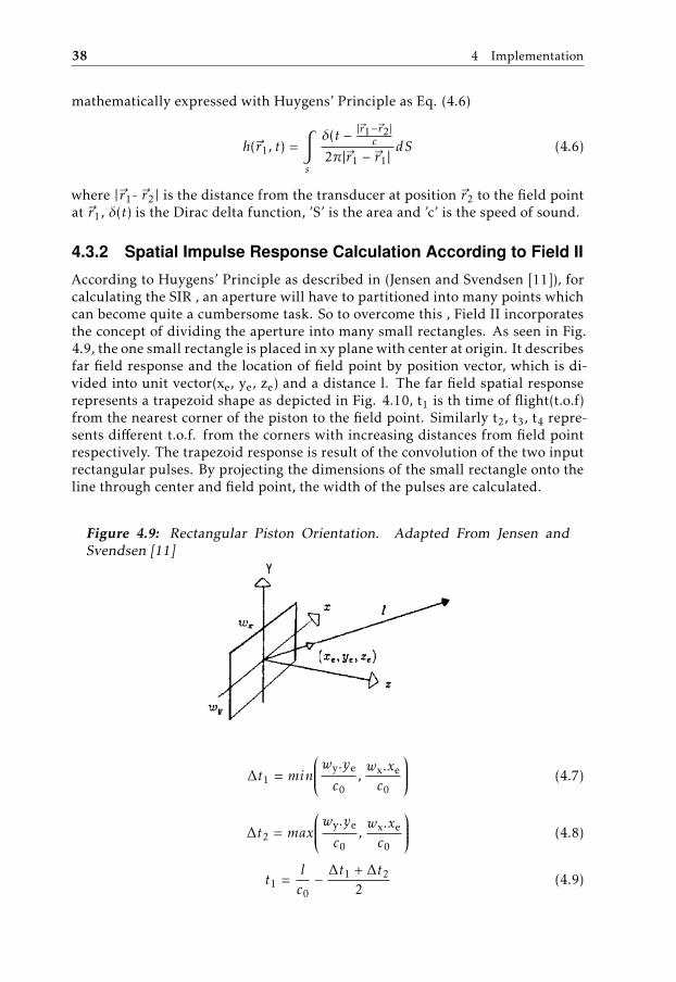
4.3.2 Spatial Impulse Response Calculation According to Field II
According to Huygens’ Principle as described in (Jensen and Svendsen [11]), forcalculating the SIR , an aperture will have to partitioned into many points whichcan become quite a cumbersome task. So to overcome this , Field II incorporatesthe concept of dividing the aperture into many small rectangles. As seen in Fig.4.9, the one small rectangle is placed in xy plane with center at origin. It describesfar field response and the location of field point by position vector, which is di-vided into unit vector(xe, ye, ze) and a distance l. The far field spatial responserepresents a trapezoid shape as depicted in Fig. 4.10, t1 is th time of flight(t.o.f)from the nearest corner of the piston to the field point. Similarly t2, t3, t4 repre-sents different t.o.f. from the corners with increasing distances from field pointrespectively. The trapezoid response is result of the convolution of the two inputrectangular pulses. By projecting the dimensions of the small rectangle onto theline through center and field point, the width of the pulses are calculated.
Figure 4.9: Rectangular Piston Orientation. Adapted From Jensen andSvendsen [11]
∆t1 = min
wy.ye
c0,wx.xe
c0
(4.7)
∆t2 = max
wy.ye
c0,wx.xe
c0
(4.8)
t1 =lc0− ∆t1 + ∆t2
2(4.9)

4.3 Field II 39
Figure 4.10: Far Field Response. Adapted From Jensen and Svendsen [11]
t2 = t1 + ∆t1 (4.10)
t3 = t1 + ∆t2 (4.11)
t4 = t1 + ∆t1 + ∆t2 (4.12)
where wx and wy are the side lengths of rectangle and t1,t2,t3,t4 are the arrivaltimes and area of the trapezoid is given by Eq. (4.13)
arec(l) =wx.wy
2πl(4.13)


5Results and Inferences
This section elucidates the simulation results that were obtained while runningthe simulation tests on Field II and modified TAC GUI. The parameters whichwere simulated in Field II are as follows: single element array transducer and itscorresponding parameters, an array of transducers and its parameters, SIR andpressure along the axis for array of transducers, pressure along radial line, pres-sure field in xz plane, apodization concept addition, sensitivity of the receiverarray and dynamic focusing, pulse echo response and grating lobes for the arrayof transducers. The results comprises of Matlab coding and its correspondingsimulated graphs for the parameters set by us.
The later part of the result section displays the simulation results om TACGUI. It displays the directivity plots, near field region, far field region, hapticsfor various configurations of transducer parameters.
41
42 5 Results and Inferences
5.1 Field II Simulations
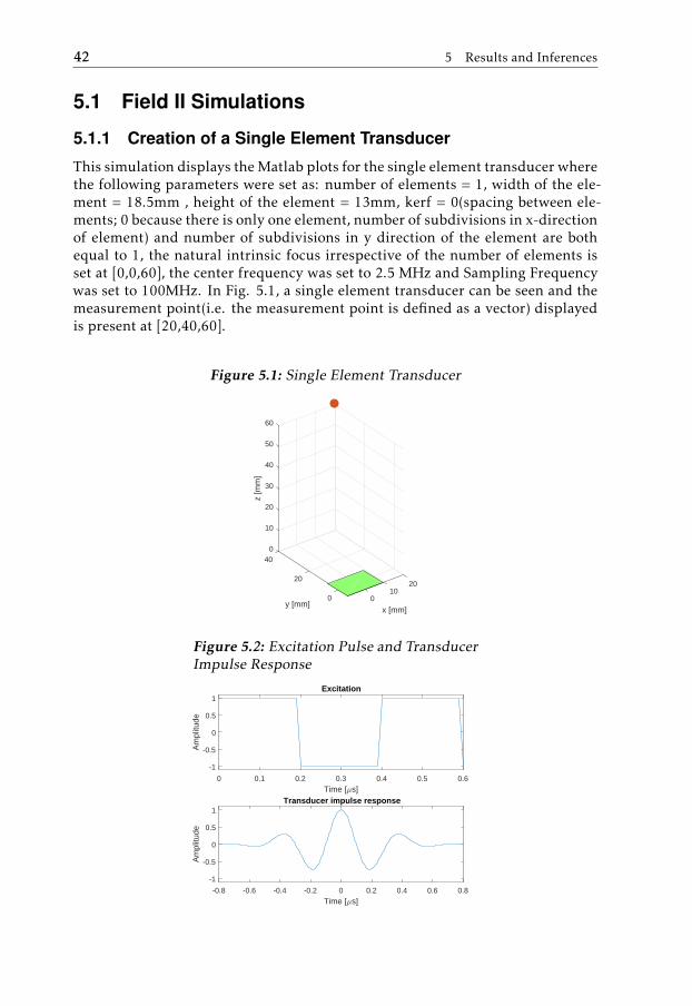
5.1.1 Creation of a Single Element Transducer
This simulation displays the Matlab plots for the single element transducer wherethe following parameters were set as: number of elements = 1, width of the ele-ment = 18.5mm , height of the element = 13mm, kerf = 0(spacing between ele-ments; 0 because there is only one element, number of subdivisions in x-directionof element) and number of subdivisions in y direction of the element are bothequal to 1, the natural intrinsic focus irrespective of the number of elements isset at [0,0,60], the center frequency was set to 2.5 MHz and Sampling Frequencywas set to 100MHz. In Fig. 5.1, a single element transducer can be seen and themeasurement point(i.e. the measurement point is defined as a vector) displayedis present at [20,40,60].
Figure 5.1: Single Element Transducer
040
10
20
30
z [m
m]
20
y [mm]
40
20
50
10
x [mm]
60
0 0
Figure 5.2: Excitation Pulse and TransducerImpulse Response
0 0.1 0.2 0.3 0.4 0.5 0.6
Time [ s]
-1
-0.5
0
0.5
1
Am
plitu
de
Excitation
-0.8 -0.6 -0.4 -0.2 0 0.2 0.4 0.6 0.8
Time [ s]
-1
-0.5
0
0.5
1
Am
plitu
de
Transducer impulse response
5.1 Field II Simulations 43
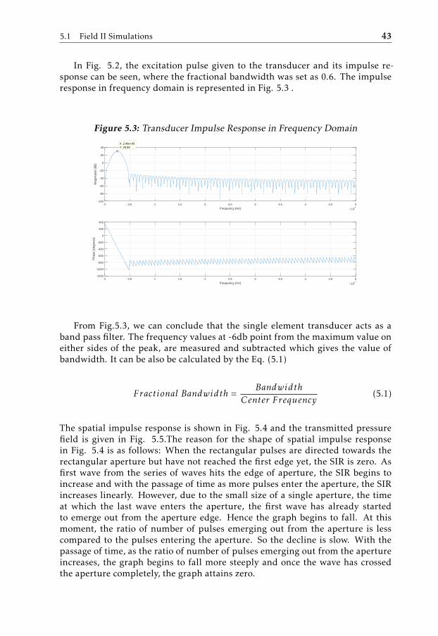
In Fig. 5.2, the excitation pulse given to the transducer and its impulse re-sponse can be seen, where the fractional bandwidth was set as 0.6. The impulseresponse in frequency domain is represented in Fig. 5.3 .
Figure 5.3: Transducer Impulse Response in Frequency Domain
0 0.5 1 1.5 2 2.5 3 3.5 4 4.5 5
Frequency (Hz) 107
-1200
-1000
-800
-600
-400
-200
0
200
400
Pha
se (
degr
ees)
0 0.5 1 1.5 2 2.5 3 3.5 4 4.5 5
Frequency (Hz) 107
-100
-80
-60
-40
-20
0
20
40
Mag
nitu
de (
dB)
X: 2.49e+06Y: 29.89
From Fig.5.3, we can conclude that the single element transducer acts as aband pass filter. The frequency values at -6db point from the maximum value oneither sides of the peak, are measured and subtracted which gives the value ofbandwidth. It can be also be calculated by the Eq. (5.1)
Fractional Bandwidth =Bandwidth
Center Frequency(5.1)
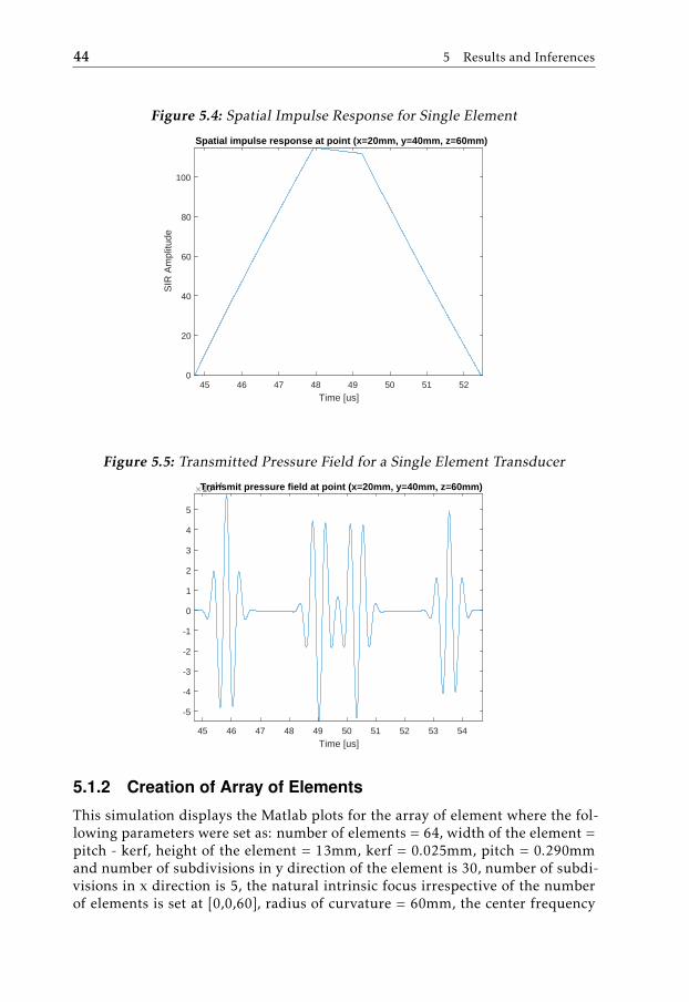
The spatial impulse response is shown in Fig. 5.4 and the transmitted pressurefield is given in Fig. 5.5.The reason for the shape of spatial impulse responsein Fig. 5.4 is as follows: When the rectangular pulses are directed towards therectangular aperture but have not reached the first edge yet, the SIR is zero. Asfirst wave from the series of waves hits the edge of aperture, the SIR begins toincrease and with the passage of time as more pulses enter the aperture, the SIRincreases linearly. However, due to the small size of a single aperture, the timeat which the last wave enters the aperture, the first wave has already startedto emerge out from the aperture edge. Hence the graph begins to fall. At thismoment, the ratio of number of pulses emerging out from the aperture is lesscompared to the pulses entering the aperture. So the decline is slow. With thepassage of time, as the ratio of number of pulses emerging out from the apertureincreases, the graph begins to fall more steeply and once the wave has crossedthe aperture completely, the graph attains zero.
44 5 Results and Inferences
Figure 5.4: Spatial Impulse Response for Single Element
45 46 47 48 49 50 51 52
Time [us]
0
20
40
60
80
100S
IR A
mpl
itude
Spatial impulse response at point (x=20mm, y=40mm, z=60mm)
Figure 5.5: Transmitted Pressure Field for a Single Element Transducer
45 46 47 48 49 50 51 52 53 54
Time [us]
-5
-4
-3
-2
-1
0
1
2
3
4
5
10-14Transmit pressure field at point (x=20mm, y=40mm, z=60mm)
5.1.2 Creation of Array of Elements
This simulation displays the Matlab plots for the array of element where the fol-lowing parameters were set as: number of elements = 64, width of the element =pitch - kerf, height of the element = 13mm, kerf = 0.025mm, pitch = 0.290mmand number of subdivisions in y direction of the element is 30, number of subdi-visions in x direction is 5, the natural intrinsic focus irrespective of the numberof elements is set at [0,0,60], radius of curvature = 60mm, the center frequency
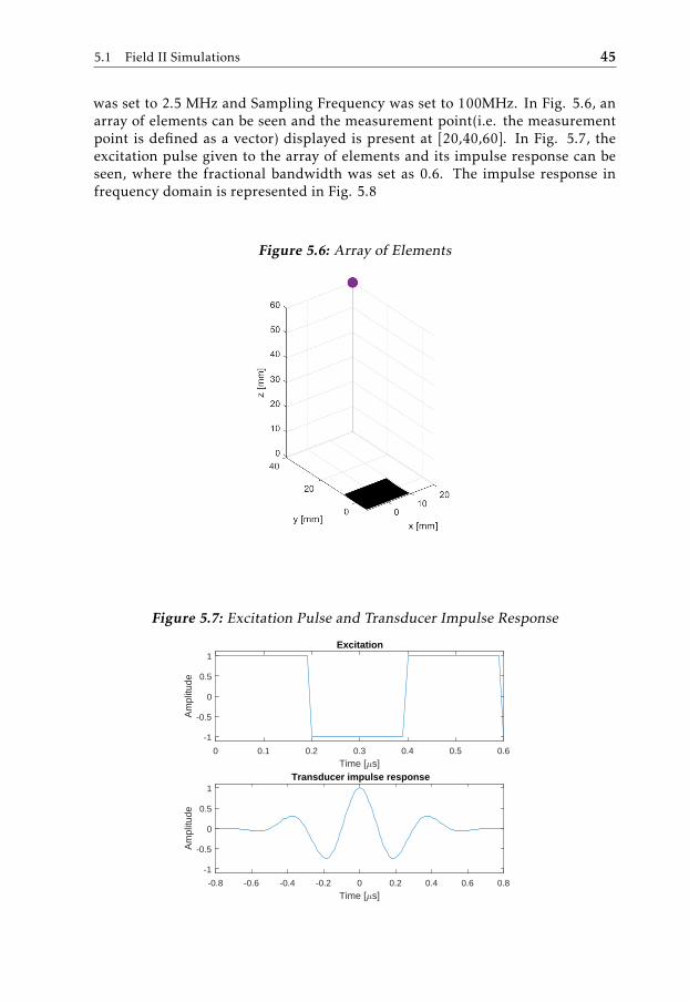
5.1 Field II Simulations 45
was set to 2.5 MHz and Sampling Frequency was set to 100MHz. In Fig. 5.6, anarray of elements can be seen and the measurement point(i.e. the measurementpoint is defined as a vector) displayed is present at [20,40,60]. In Fig. 5.7, theexcitation pulse given to the array of elements and its impulse response can beseen, where the fractional bandwidth was set as 0.6. The impulse response infrequency domain is represented in Fig. 5.8
Figure 5.6: Array of Elements
Figure 5.7: Excitation Pulse and Transducer Impulse Response
0 0.1 0.2 0.3 0.4 0.5 0.6
Time [ s]
-1
-0.5
0
0.5
1
Am
plitu
de
Excitation
-0.8 -0.6 -0.4 -0.2 0 0.2 0.4 0.6 0.8
Time [ s]
-1
-0.5
0
0.5
1
Am
plitu
de
Transducer impulse response
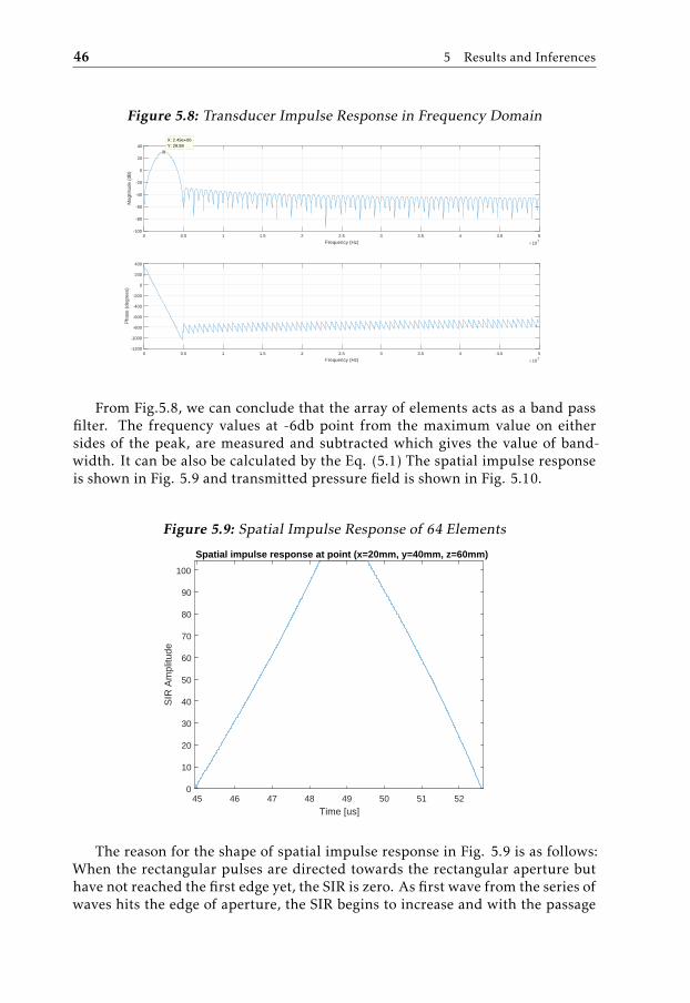
46 5 Results and Inferences
Figure 5.8: Transducer Impulse Response in Frequency Domain
0 0.5 1 1.5 2 2.5 3 3.5 4 4.5 5
Frequency (Hz) 107
-1200
-1000
-800
-600
-400
-200
0
200
400
Pha
se (
degr
ees)
0 0.5 1 1.5 2 2.5 3 3.5 4 4.5 5
Frequency (Hz) 107
-100
-80
-60
-40
-20
0
20
40
Mag
nitu
de (
dB)
X: 2.49e+06Y: 29.89
From Fig.5.8, we can conclude that the array of elements acts as a band passfilter. The frequency values at -6db point from the maximum value on eithersides of the peak, are measured and subtracted which gives the value of band-width. It can be also be calculated by the Eq. (5.1) The spatial impulse responseis shown in Fig. 5.9 and transmitted pressure field is shown in Fig. 5.10.
Figure 5.9: Spatial Impulse Response of 64 Elements
45 46 47 48 49 50 51 52
Time [us]
0
10
20
30
40
50
60
70
80
90
100
SIR
Am
plitu
de
Spatial impulse response at point (x=20mm, y=40mm, z=60mm)
The reason for the shape of spatial impulse response in Fig. 5.9 is as follows:When the rectangular pulses are directed towards the rectangular aperture buthave not reached the first edge yet, the SIR is zero. As first wave from the series ofwaves hits the edge of aperture, the SIR begins to increase and with the passage
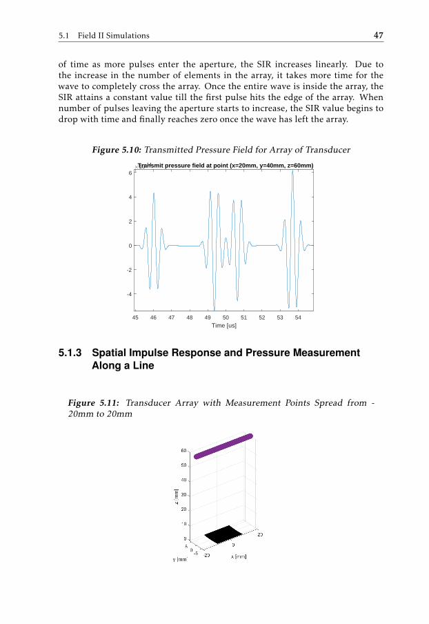
5.1 Field II Simulations 47
of time as more pulses enter the aperture, the SIR increases linearly. Due tothe increase in the number of elements in the array, it takes more time for thewave to completely cross the array. Once the entire wave is inside the array, theSIR attains a constant value till the first pulse hits the edge of the array. Whennumber of pulses leaving the aperture starts to increase, the SIR value begins todrop with time and finally reaches zero once the wave has left the array.
Figure 5.10: Transmitted Pressure Field for Array of Transducer
45 46 47 48 49 50 51 52 53 54
Time [us]
-4
-2
0
2
4
610-14Transmit pressure field at point (x=20mm, y=40mm, z=60mm)
5.1.3 Spatial Impulse Response and Pressure MeasurementAlong a Line
Figure 5.11: Transducer Array with Measurement Points Spread from -20mm to 20mm
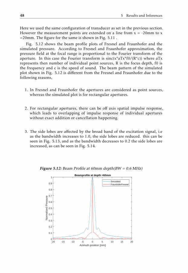
48 5 Results and Inferences
Here we used the same configuration of transducer as set in the previous section.However the measurement points are extended on a line from x = -20mm to x=20mm. The figure for the same is shown in Fig. 5.11 .
Fig. 5.12 shows the beam profile plots of Fresnel and Fraunhofer and thesimulated pressure. According to Fresnel and Fraunhofer approximation, thepressure field at the focal range is proportional to the Fourier transform of theaperture. In this case the Fourier transform is sinc(x*aTx*f0/(R*c)) where aTxrepresents then number of individual point sources, R is the focus depth, f0 isthe frequency and c is the speed of sound. The beam pattern of the simulatedplot shown in Fig. 5.12 is different from the Fresnel and Fraunhofer due to thefollowing reasons,
1. In Fresnel and Fraunhofer the apertures are considered as point sources,whereas the simulated plot is for rectangular apertures.
2. For rectangular apertures, there can be off axis spatial impulse response,which leads to overlapping of impulse response of individual apertureswithout exact addition or cancellation happening.
3. The side lobes are affected by the broad band of the excitation signal, i.eas the bandwidth increases to 1.0, the side lobes are reduced. this can beseen in Fig. 5.13, and as the bandwidth decreases to 0.2 the side lobes areincreased, as can be seen in Fig. 5.14.
Figure 5.12: Beam Profile at 60mm depth(BW = 0.6 MHz)
-20 -15 -10 -5 0 5 10 15 20
Azimuth position [mm]
0
0.1
0.2
0.3
0.4
0.5
0.6
0.7
0.8
0.9
1
Nor
mal
ized
Pre
ssur
e
Beamprofile at depth =60mm
SimulatedFraunhoferFresnel
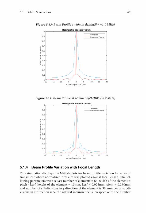
5.1 Field II Simulations 49
Figure 5.13: Beam Profile at 60mm depth(BW =1.0 MHz)
-20 -15 -10 -5 0 5 10 15 20
Azimuth position [mm]
0
0.1
0.2
0.3
0.4
0.5
0.6
0.7
0.8
0.9
1
Nor
mal
ized
Pre
ssur
e
Beamprofile at depth =60mm
SimulatedFraunhoferFresnel
Figure 5.14: Beam Profile at 60mm depth(BW = 0.2 MHz)
-20 -15 -10 -5 0 5 10 15 20
Azimuth position [mm]
0
0.1
0.2
0.3
0.4
0.5
0.6
0.7
0.8
0.9
1
Nor
mal
ized
Pre
ssur
e
Beamprofile at depth =60mm
SimulatedFraunhoferFresnel
5.1.4 Beam Profile Variation with Focal Length
This simulation displays the Matlab plots for beam profile variation for array oftransducer where normalized pressure was plotted against focal length. The fol-lowing parameters were set as: number of elements = 64, width of the element =pitch - kerf, height of the element = 13mm, kerf = 0.025mm, pitch = 0.290mmand number of subdivisions in y direction of the element is 30, number of subdi-visions in x direction is 5, the natural intrinsic focus irrespective of the number
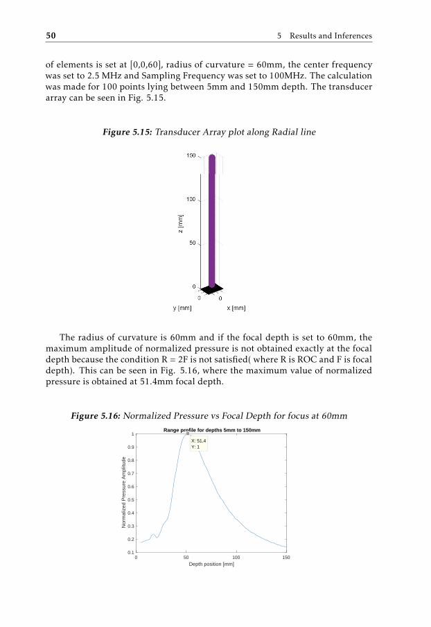
50 5 Results and Inferences
of elements is set at [0,0,60], radius of curvature = 60mm, the center frequencywas set to 2.5 MHz and Sampling Frequency was set to 100MHz. The calculationwas made for 100 points lying between 5mm and 150mm depth. The transducerarray can be seen in Fig. 5.15.
Figure 5.15: Transducer Array plot along Radial line
The radius of curvature is 60mm and if the focal depth is set to 60mm, themaximum amplitude of normalized pressure is not obtained exactly at the focaldepth because the condition R = 2F is not satisfied( where R is ROC and F is focaldepth). This can be seen in Fig. 5.16, where the maximum value of normalizedpressure is obtained at 51.4mm focal depth.
Figure 5.16: Normalized Pressure vs Focal Depth for focus at 60mm
0 50 100 150
Depth position [mm]
0.1
0.2
0.3
0.4
0.5
0.6
0.7
0.8
0.9
1
Nor
mal
ized
Pre
ssur
e A
mpl
itude
Range profile for depths 5mm to 150mm
X: 51.4Y: 1

5.1 Field II Simulations 51
Figure 5.17: Normalized Pressure vs Focal Depth for focus at 30mm
0 50 100 150
Depth position [mm]
0
0.1
0.2
0.3
0.4
0.5
0.6
0.7
0.8
0.9
1
Nor
mal
ized
Pre
ssur
e A
mpl
itude
Range profile for depths 5mm to 150mm
X: 31.1Y: 1
Instead if we set the value of F to 30mm, the condition gets satisfied andmaximum pressure amplitude is obtained at approximately 30mm focal depth.This is seen in Fig. 5.17
5.1.5 Apodization
Figure 5.18: Transmit Beam Pressure Field in Whole XZ plane withoutapodization
Apodization is the technique used to reduce the strength of the side lobes, whichare formed during the focusing of ultrasound. The amplitude across the aperture
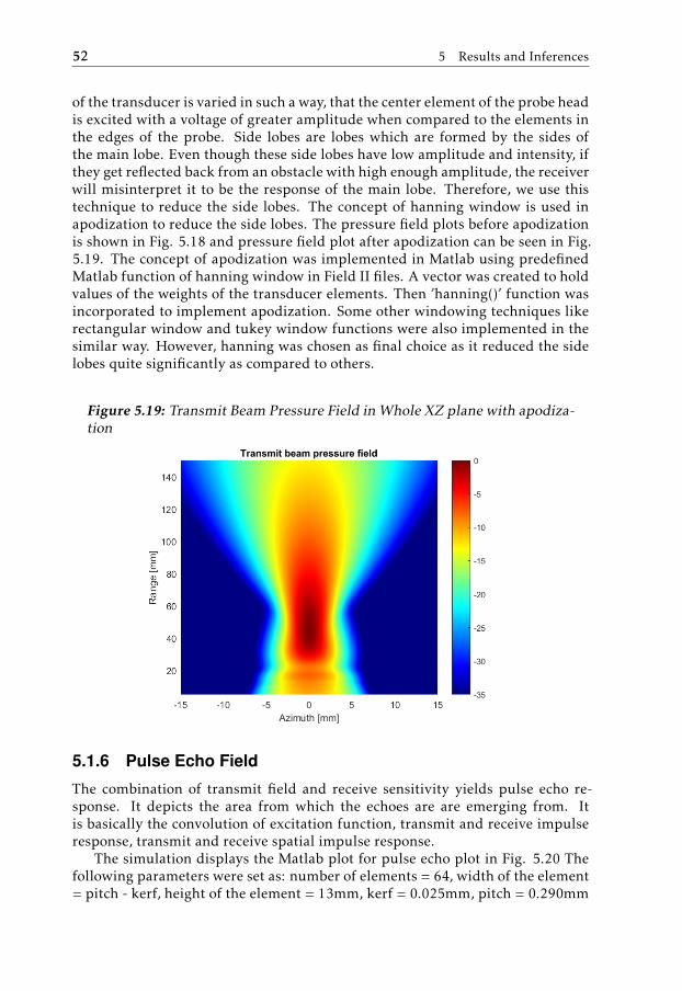
52 5 Results and Inferences
of the transducer is varied in such a way, that the center element of the probe headis excited with a voltage of greater amplitude when compared to the elements inthe edges of the probe. Side lobes are lobes which are formed by the sides ofthe main lobe. Even though these side lobes have low amplitude and intensity, ifthey get reflected back from an obstacle with high enough amplitude, the receiverwill misinterpret it to be the response of the main lobe. Therefore, we use thistechnique to reduce the side lobes. The concept of hanning window is used inapodization to reduce the side lobes. The pressure field plots before apodizationis shown in Fig. 5.18 and pressure field plot after apodization can be seen in Fig.5.19. The concept of apodization was implemented in Matlab using predefinedMatlab function of hanning window in Field II files. A vector was created to holdvalues of the weights of the transducer elements. Then ’hanning()’ function wasincorporated to implement apodization. Some other windowing techniques likerectangular window and tukey window functions were also implemented in thesimilar way. However, hanning was chosen as final choice as it reduced the sidelobes quite significantly as compared to others.
Figure 5.19: Transmit Beam Pressure Field in Whole XZ plane with apodiza-tion
5.1.6 Pulse Echo Field
The combination of transmit field and receive sensitivity yields pulse echo re-sponse. It depicts the area from which the echoes are are emerging from. Itis basically the convolution of excitation function, transmit and receive impulseresponse, transmit and receive spatial impulse response.
The simulation displays the Matlab plot for pulse echo plot in Fig. 5.20 Thefollowing parameters were set as: number of elements = 64, width of the element= pitch - kerf, height of the element = 13mm, kerf = 0.025mm, pitch = 0.290mm
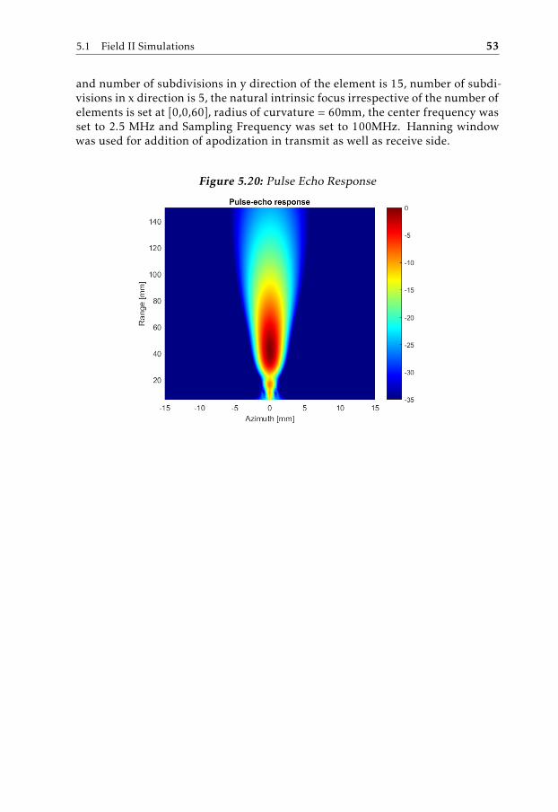
5.1 Field II Simulations 53
and number of subdivisions in y direction of the element is 15, number of subdi-visions in x direction is 5, the natural intrinsic focus irrespective of the number ofelements is set at [0,0,60], radius of curvature = 60mm, the center frequency wasset to 2.5 MHz and Sampling Frequency was set to 100MHz. Hanning windowwas used for addition of apodization in transmit as well as receive side.
Figure 5.20: Pulse Echo Response
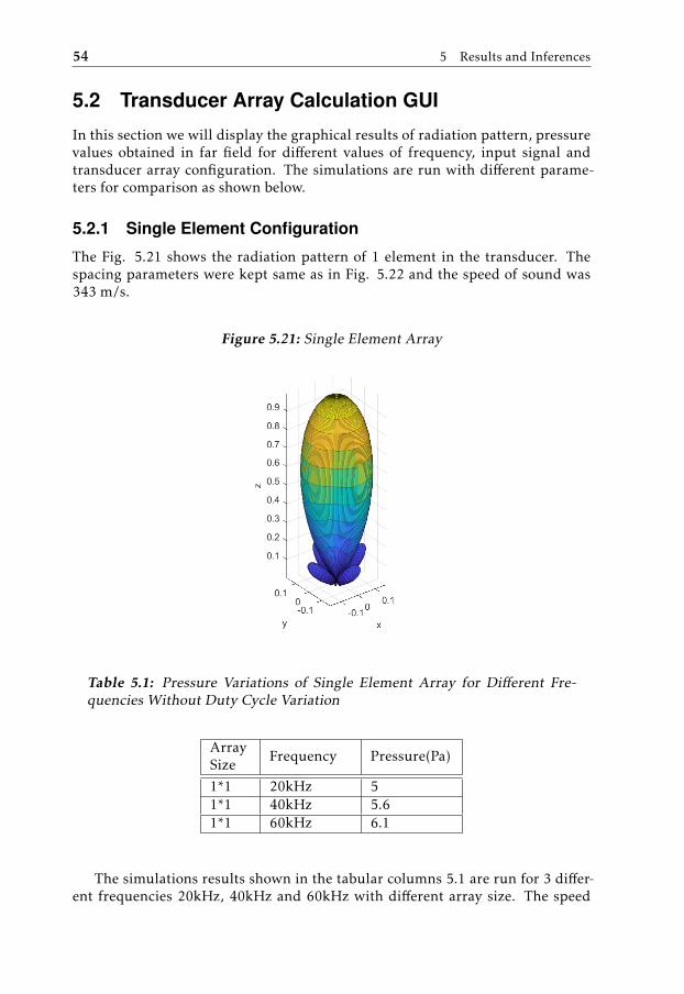
54 5 Results and Inferences
5.2 Transducer Array Calculation GUI
In this section we will display the graphical results of radiation pattern, pressurevalues obtained in far field for different values of frequency, input signal andtransducer array configuration. The simulations are run with different parame-ters for comparison as shown below.
5.2.1 Single Element Configuration
The Fig. 5.21 shows the radiation pattern of 1 element in the transducer. Thespacing parameters were kept same as in Fig. 5.22 and the speed of sound was343 m/s.
Figure 5.21: Single Element Array
Table 5.1: Pressure Variations of Single Element Array for Different Fre-quencies Without Duty Cycle Variation
ArraySize
Frequency Pressure(Pa)
1*1 20kHz 51*1 40kHz 5.61*1 60kHz 6.1
The simulations results shown in the tabular columns 5.1 are run for 3 differ-ent frequencies 20kHz, 40kHz and 60kHz with different array size. The speed

5.2 Transducer Array Calculation GUI 55
of sound is kept constant (343m/s) and the pressure and intensity values are ob-tained at a distance of 5cm from the array. All the other spacing parameters werekept same as Fig. 5.22
5.2.2 Comparison of Multi Element Array
In this subsection the element array configuration that we used initially can beseen in Fig. 5.22. This configuration was given an input signal of 20 Khz squaresignal.
Figure 5.22: Element Array Configuration
The corresponding radiation pattern can be seen in Fig. 5.23.
Figure 5.23: Radiation Pattern of 3*3 Matrix
As seen in Fig.5.23 the radiation pattern is for a 3*3 matrix array, which showsthe maximum Z distance(cm) at which the pressure can be felt. The radiation pat-tern in Fig. 5.27 is obtained for a 6*6 matrix by changing the number of elements

56 5 Results and Inferences
in the transducer array configuration. From these two graphs it can be clearlyseen that by increasing the number of elements in the matrix(keeping other pa-rameters constant), it is possible to obtain the pressure at a much higher distance.
Figure 5.24: Radiation Pattern of 6*6 Matrix
The far field regions of 3*3 and 6*6 matrix is seen in Fig. 5.29 and Fig. 6.1respectively.
Figure 5.25: Far Field Region of 3*3 Matrix
0 0.02 0.04 0.06 0.08 0.1 0.12
z in [m]
0
500
1000
1500
2000
2500
abs
(Pre
ssur
e)
Field Region
X: 0.1Y: 22.91
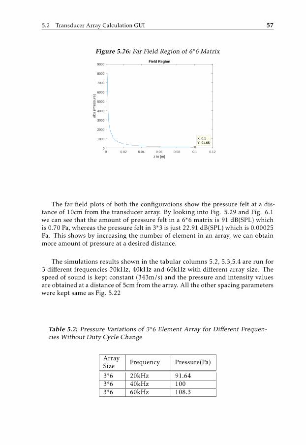
5.2 Transducer Array Calculation GUI 57
Figure 5.26: Far Field Region of 6*6 Matrix
0 0.02 0.04 0.06 0.08 0.1 0.12
z in [m]
0
1000
2000
3000
4000
5000
6000
7000
8000
9000
abs
(Pre
ssur
e)
Field Region
X: 0.1Y: 91.65
The far field plots of both the configurations show the pressure felt at a dis-tance of 10cm from the transducer array. By looking into Fig. 5.29 and Fig. 6.1we can see that the amount of pressure felt in a 6*6 matrix is 91 dB(SPL) whichis 0.70 Pa, whereas the pressure felt in 3*3 is just 22.91 dB(SPL) which is 0.00025Pa. This shows by increasing the number of element in an array, we can obtainmore amount of pressure at a desired distance.
The simulations results shown in the tabular columns 5.2, 5.3,5.4 are run for3 different frequencies 20kHz, 40kHz and 60kHz with different array size. Thespeed of sound is kept constant (343m/s) and the pressure and intensity valuesare obtained at a distance of 5cm from the array. All the other spacing parameterswere kept same as Fig. 5.22
Table 5.2: Pressure Variations of 3*6 Element Array for Different Frequen-cies Without Duty Cycle Change
ArraySize
Frequency Pressure(Pa)
3*6 20kHz 91.643*6 40kHz 1003*6 60kHz 108.3
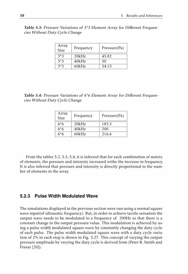
58 5 Results and Inferences
Table 5.3: Pressure Variations of 3*3 Element Array for Different Frequen-cies Without Duty Cycle Change
ArraySize
Frequency Pressure(Pa)
3*3 20kHz 45.823*3 40kHz 503*3 60kHz 54.15
Table 5.4: Pressure Variations of 6*6 Element Array for Different Frequen-cies Without Duty Cycle Change
ArraySize
Frequency Pressure(Pa)
6*6 20kHz 183.36*6 40kHz 2006*6 60kHz 216.6
From the tables 5.2, 5.3, 5.4, it is inferred that for each combination of matrixof elements, the pressure and intensity increased withe the increase in frequency.It is also inferred that pressure and intensity is directly proportional to the num-ber of elements in the array.
5.2.3 Pulse Width Modulated Wave
The simulations displayed in the previous section were run using a normal squarewave input(of ultrasonic frequency). But, in order to achieve tactile sensation theoutput wave needs to be modulated to a frequency of 200Hz so that there is aconstant change in the output pressure value. This modulation is achieved by us-ing a pulse width modulated square wave by constantly changing the duty cycleof each pulse. The pulse width modulated square wave with a duty cycle varia-tion of 2% in each step is shown in Fig. 5.27. This concept of varying the outputpressure amplitude by varying the duty cycle is derived from (Peter R. Smith andFreear [20]).

5.2 Transducer Array Calculation GUI 59
Figure 5.27: Pulse Width Modulated Square Wave
2 4 6 8 10 12 14 16
Time(in s) 10-4
-3
-2
-1
0
1
2
3A
mpl
itude
When the PWM signal is given as input to the transducer, the output pres-sure of the sound wave varies constantly, showing that the output pressure isproportional to the width of the pulse. But, the change in pressure is not directlyor linearly proportional to the width of the pulse. According to (Peter R. Smithand Freear [20]) a linear relationship between pulse width and pressure outputdoes not exist; a percentage increase in pulse width does not provide the samepercentage increase in output pressure. On contrary when we consider a linearrelationship between pulse width and amplitude, the variation in amplitude ofthe output wave with respect to input, can be seen in Fig. 5.28.
Figure 5.28: Amplitude Modulation using PWM
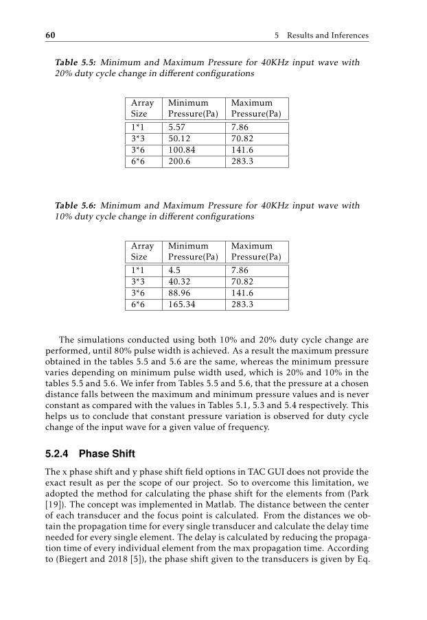
60 5 Results and Inferences
Table 5.5: Minimum and Maximum Pressure for 40KHz input wave with20% duty cycle change in different configurations
ArraySize
MinimumPressure(Pa)
MaximumPressure(Pa)
1*1 5.57 7.863*3 50.12 70.823*6 100.84 141.66*6 200.6 283.3
Table 5.6: Minimum and Maximum Pressure for 40KHz input wave with10% duty cycle change in different configurations
ArraySize
MinimumPressure(Pa)
MaximumPressure(Pa)
1*1 4.5 7.863*3 40.32 70.823*6 88.96 141.66*6 165.34 283.3
The simulations conducted using both 10% and 20% duty cycle change areperformed, until 80% pulse width is achieved. As a result the maximum pressureobtained in the tables 5.5 and 5.6 are the same, whereas the minimum pressurevaries depending on minimum pulse width used, which is 20% and 10% in thetables 5.5 and 5.6. We infer from Tables 5.5 and 5.6, that the pressure at a chosendistance falls between the maximum and minimum pressure values and is neverconstant as compared with the values in Tables 5.1, 5.3 and 5.4 respectively. Thishelps us to conclude that constant pressure variation is observed for duty cyclechange of the input wave for a given value of frequency.
5.2.4 Phase Shift
The x phase shift and y phase shift field options in TAC GUI does not provide theexact result as per the scope of our project. So to overcome this limitation, weadopted the method for calculating the phase shift for the elements from (Park[19]). The concept was implemented in Matlab. The distance between the centerof each transducer and the focus point is calculated. From the distances we ob-tain the propagation time for every single transducer and calculate the delay timeneeded for every single element. The delay is calculated by reducing the propaga-tion time of every individual element from the max propagation time. Accordingto (Biegert and 2018 [5]), the phase shift given to the transducers is given by Eq.

5.2 Transducer Array Calculation GUI 61
(5.2)φ = 2.π.f .δt (5.2)
where φ is the phase shift, f is the transmit frequency and δt is the time delayof the signal for each element.
Figure 5.29: 3*3 circular transducers
A 3*3 square array of circular transducer with the point of focus representedby a blue point is shown in Fig.5.29. The coordinate points are [0.01,0.01,100e-3]m. The phase shift values obtained from the time delay using Eq. (5.2) are shownin the tabular column 5.7
Table 5.7: Phase Shift Values for 3*3 Matrix
TransducerNumber
Delay(in µs)PhaseShift(indeg)
1 5.9384 85.512 10.547 151.873 11.998 172.774 4.5174 655 9.1040 1316 10.547 151.877 0 08 4.5174 659 5.9384 85.5
It can be seen from the table 5.7 that the transducer farthest(i.e 7) from thepoint of focus needs the least delay. This is because, it has the maximum propaga-

62 5 Results and Inferences
tion time for the sound wave to reach the point of focus. However, the transducerclosest to the point of focus (i.e 3) has the maximum time delay.

6Conclusion
6.1 Thesis Contribution
The initial part of the thesis constitutes the understanding of characteristics andworking principles of an Ultrasonic Transducer. The next section involves theresearch on Haptic feedback using ultrasonic transducers. This provides us theinsight of the principles that govern haptics.
For validating the characteristics of transducer we used Field II simulationtool. In this, we initially measured the impulse responses of single element andmulti element transducer in both time as well as frequency domain. With theirfrequency domain analysis we concluded that both, the single and multi elementtransducer act as band pass filter. This can be seen from Fig. 5.3 and 5.8. Next,we simulated transducer beam profile for a multi element array and comparedit with Fresnel and Fraunhofer approximation. The simulated beam profile wasmuch wider then the Fresnel and Fraunhofer beam profile. It was also observedthat with the increase in bandwidth of the input signal of a transducer, the sidelobes in the beam profile plot can be reduced. The beam profile was then simu-lated with focal length to observe the variation in pressure at various focal depth.It gave a clear validation that the maximum pressure was obtained when ROC isequal to twice the focal length. The concept of apodization was validated usinghanning window to reduce the number of side lobes in the pressure field. Thiscomparison is shown in Fig. 5.18 and 5.19.
A Matlab based GUI was also used to perform simulations of transducer pres-sure field. The pressure field simulations were conducted for single element aswell as multi element array. By observing the pressure plots and the comparingtheir pressure and intensity values, it is unambiguous to say that by increasingthe number of elements and frequency of the input signal of the transducer, thepressure and intensity values increases. Furthermore, the far field pressure plots
63
64 6 Conclusion
for various configurations also proves that by increasing the distance of the fo-cus from the array the pressure value decreases. The above mentioned analyseswere simulated for both normal square wave input as well as pulse width mod-ulated wave. The concept of phase shift and delay were implemented in Matlabwhich demonstrated that by changing these values the point of focus for beamformation can be altered by the user.
6.2 Future Work
The field of haptics is very interesting and is growing rapidly. The research pre-sented in this paper can form the basis for the following areas in future:
1. Development of electronics hardware, which will involve the concepts ofduty cycle variation and amplitude modulation presented by the researchwork. The guidance for the electronics can be derived from Asier Marzoand Drinkwater [1].
2. Merging of the phase shift concept presented in the thesis research workalong with the TAC GUI. This could be done to obtain dynamic relationshipbetween time and acoustic pressure variation.
3. The thesis research work could provide the requisite knowledge for anyaspirant who wants to continue the topic as a PhD research.

6.3 License for using TAC GUI 65
6.3 License for using TAC GUI
The following license was obtained for using TAC GUI in our thesis work. The li-cense copy can be found in https://se.mathworks.com/matlabcentral/fileexchange/35657-transducer-array-calculation-tac-gui.
Figure 6.1: license Agreement

Bibliography
[1] Tom Corkett Asier Marzo and Bruce W. Drinkwater. Ultraino: An openphased-array system for narrowband airborne ultrasound transmission. Vol-ume 65, No. 1:Pages 102–111, January 2018. Cited on pages 19, 27, and 64.
[2] Katherine Asztalos. Design and development of a nasal inhaler. 2016.URL https://www.researchgate.net/profile/Katherine_Asztalos/publication/317701554_Design_and_Development_of_a_Nasal_Inhaler/links/594992e90f7e9b0d85230b30/Design-and-Development-of-a-Nasal-Inhaler.pdf?origin=publication_detail. Cited on pages 8 and 9.
[3] Tom Carter Sriram Subramanian Benjamin Long, Sue Ann Seah. Renderingvolumetric haptic shapes in mid air using ultrasound. Cited on pages 4, 20,24, 25, 26, and 27.
[4] Nonlinear Acoustics Beyer. The acoustic wave equation and simple solu-tions. 1974. Cited on page 18.
[5] Mark Biegert and Math Encounters 2018. Beamforming math. 20 January2012. Cited on pages 22 and 60.
[6] NDT Education Resource Center. The collaboration for ndt education. 2001-2014. URL www.ndt-ed.org. Cited on pages 5, 6, 7, and 12.
[7] Qinxue Pan Chunguang Xu Chunyan Gao, Dingguo Xiao. Ultrasonic trans-ducers frequency response study with equivalent circuit and finite elementmethod. 2011. Cited on pages 9 and 10.
[8] Charles A. Cain Emad S. Ebbini. Multiple-focus ultrasound phased-arraypattern synthesis: Optimal driving-signal distributions for hyperthermia.Vol.36, No.5, September 1989. Cited on page 25.
[9] G.E.Tupholme. Generation of acoustic pulses by baffled plane pistons.Vol.16, 1969. Cited on page 36.
67

68 Bibliography
[10] Jorgen Arendt Jensen. Simulation of advanced ultrasound systems usingfield ii. Center fo Fast Ultrasound Imaging, Technical University of Den-mark, 2004. Cited on page 37.
[11] Jorgen Arendt Jensen and Niels Bruun Svendsen. Calculation of pressurefields from arbitrarily shaped, apodized, and excited ultrasound transduc-ers. IEEE TRANSACTIONS ON ULTRASONICS. FERROELECTRICS. ANDFREQUENCY CONTROL. Cited on pages 38 and 39.
[12] Jørgen Arendt Jensen. Linear description of ultrasound imaging systems.June 1999. Cited on pages 36 and 37.
[13] Cheoljin Lee Kerem Karadayi and Yongmin Kim. Software-based ultrasound beamforming on multi-core dsps. Im-age Computing Systems Laboratory., 2011. URLDepartmentsofElectricalEngineeringandBioengineering.Cited on pages 23 and 24.
[14] Benedikt Kohout. Transducer array calculation gui. Ver-sion 1.9.0.0, 12th September 2012. URL https://se.mathworks.com/matlabcentral/fileexchange/35657-transducer-array-calculation-tac-gui. Cited onpages 32, 33, and 34.
[15] Fredrick W. Kremkau. Multiple element transducers. 13. Cited on page 13.
[16] Eduardo Moreno M. Castillo, P. Acevedo. Klm model for lossy piezoelectrictransducers. pages Pages 671–679, 2003. URL www-sciencedirect-com.Cited on page 10.
[17] J. Podobnik M. Mihelj. Haptics for virtual reality and teleoperation, intel-ligent systems, control and automation: Science and engineering 64. Citedon pages 3, 15, and 16.
[18] Olympus NDT. Ultrasonic transducers technical notes. 2006. Cited on pages5 and 12.
[19] Hyo Won Park. Modeling and simulation of acoustic pressure field forultrasonic tactile displays. Theses and Dissertations. 2934., 2017. URLhttps://preserve.lehigh.edu/etd/2934. Cited on pages 19, 20, 21,and 60.
[20] David M. J. Cowell Peter R. Smith and Steven Freear. Width-modulatedsquare-wave pulses for ultrasound applications. Volume 60, No. 11:Pages2244–2256, November 2013. Cited on pages 27, 29, 58, and 59.
[21] Matthew Glisson Ali Israr Rajinder Sodhi, Ivan Poupyrev. Aireal: Interactivetactile experiences in free air. Cited on pages 17 and 18.
Bibliography 69
[22] J M. Thijssen S J H. Kervel. A calculation scheme for the optimum de-sign of ultrasonic transducers. Volume 21:Pages 134–140, May 2011. URLwww-sciencedirect-com. Cited on page 10.
[23] P. R. Stepanishen. Transient radiation from pistons in an infinite planarbaffle. Vol.49, 1971. Cited on page 36.
[24] Efland; Paul J. Roeder Pittsboro; Thomas R. Poulin Cary Stephen W. Smith,Durham; Olaf T. von Ramm. Ultrasonic transducer array. Cited on page 13.
[25] Hyongmin Lee Hyunsook Lee Heewon Kim Eunhee Shin Taehoon Kim,Sangmin Shin and Suhwan Kim. Matlab/simulink pulse-echo ultrasoundsystem simulator based on experimentally validated models. pages Pages290–291, February 2016. Cited on pages 12 and 13.
[26] Iowa State University. Radiation field of ultrasonic transducers. The Collab-oration for NDT Education, 2001-2014. URL www.ndt-ed.org. Cited onpage 11.
[27] O’Brien William D. Single element transducers. 13. Cited on page 11.
[28] RF Wireless World. Rf and wireless vendors and resources. 2012.URL http://www.rfwireless-world.com/Terminology/Analog-Beamforming-vs-Digital-Beamforming.html. Citedon page 23.