a taxonomy for classification and comparison of dataflows
TRANSCRIPT

A Taxonomy for Classification and Comparison ofDataflows for GNN Accelerators
Raveesh Garg∗, Eric Qin∗, Francisco Muñoz Matrínez†, Robert Guirado‡, Akshay Jain‡, Sergi Abadal‡,José L. Abellán§, Manuel E. Acacio†, Eduard Alarcón‡, Sivasankaran Rajamanickam¶, Tushar Krishna∗
Georgia Institute of Technology∗, Universidad de Murcia†, Universitat Politecnica de Catalunya‡
Universidad Católica de Murcia§, Sandia National Laboratories¶
Email: ∗{raveesh.g, ecqin}@gatech.edu, †{francisco.munoz2, meacacio}@um.es, ‡[email protected],‡{akshay.jain, eduard.alarcon}@upc.edu, ‡[email protected], §[email protected], ¶[email protected],
Abstract—Recently, Graph Neural Networks (GNNs) havereceived a lot of interest because of their success in learningrepresentations from graph structured data. However, GNNsexhibit different compute and memory characteristics comparedto traditional Deep Neural Networks (DNNs). Graph convolutionsrequire feature aggregations from neighboring nodes (knownas the aggregation phase), which leads to highly irregular dataaccesses. GNNs also have a very regular compute phase thatcan be broken down to matrix multiplications (known as thecombination phase). All recently proposed GNN acceleratorsutilize different dataflows and microarchitecture optimizationsfor these two phases. Different communication strategies betweenthe two phases have been also used. However, as more customGNN accelerators are proposed, the harder it is to qualitativelyclassify them and quantitatively contrast them. In this work,we present a taxonomy to describe several diverse dataflowsfor running GNN inference on accelerators. This provides astructured way to describe and compare the design-space of GNNaccelerators.
I. INTRODUCTION
Graph Neural Networks (GNNs) are gaining attention be-cause of their ability to accurately learn representations ofgraph structured data to solve graph/node classification, graphgeneration, and link prediction problems [38]. Example appli-cations include item recommendation [9], molecular featureextraction [8], natural language processing [30], semanticsegmentation [32], and fraud detection [17]. Computing GNNinference requires a mix of memory and compute intensiveoperations, which commodity CPUs, GPUs and traditionalDNN accelerators do not exploit efficiently [27], [39], [40],[44]. This led to the development of many dedicated GNNaccelerators, each with their own design methodology toextract as much performance as possible [3], [4], [11], [21],[27], [39], [41]–[43].
GNN accelerators mainly focus on accelerating two phasesthat dominate GNN inference: (1) aggregation and (2) com-bination. Aggregation phase requires irregular accesses ofdata. This is due to the irregular degree distribution in thegraphs of interest and as a result irregularity in the neighborlocations of a particular vertex in a given dataset. For example,Figure 1a shows a directed graph, and Figure 1c shows itsequivalent adjacency matrix. Since the number of vertices can
Adjacency Matrix A
1 1 0 0 00 1 1 0 00 1 1 0 11 0 0 1 01 0 0 0 1
Feature Matrix Xl
Weight Matrix W
Feature Matrix Xl+1
# Vertices: V*#
Verti
ces:
V# In Features: F
# In
Fea
ture
s: F
# Out Features: G# Out Features: G
# Ve
rtice
s: V*
# Ve
rtice
s: V
0
4 3
1
2
CSR representation of adjacency graph
# Neighbors: N*
Edge-array = [0, 1, 1, 2, 1, 2, 4, 0, 3, 0, 4]
Vertex-array = [0, 2, 4, 7, 9, 11]Vertex ID 0 1 2 3 4
Edge-ID 0 1 2 3 4 5 6 7 8 9 10
(a) (b)
(c)
Fig. 1. (a) Example graph (self loops not shown), (b) CSR repre-sentation of the adjacency matrix, (c) main computations. (Note: V*can be represented as neighbors (N*) if it is represented in CSRformat.) Any computation with A is the aggregation phase (e.g. AXor A(XW)), and any computation with W is the combination phase(e.g. XW or (AX)W).
be in the millions and the total number of edges can be inthe billions [25], accessing data efficiently is necessary forreasonable execution time. Aggregation phase can be mappedas sparse matrix × dense matrix multiplication (SpMM) withthe extremely large sparse matrix (adjacency matrix withnumber of vertices in each dimension) being the main sourceof costly irregular accesses. Combination phase computationsare similar to that of traditional DNNs. Rather than beingmemory intensive like Aggregation phase, Combination phaseis compute intensive. The main kernel for combination isdense matrix × dense matrix (GEMM). During this phase,not only the data accesses are regular, but also there are lotsof opportunities for data reuse.
Each GNN accelerator has its own unique way to computeboth Aggregation and Combination phases. This is due to threefactors: the different loop transformation choices, mappingstrategies across the processing elements, and the acceleratorarchitecture itself. The factors determine the possible dataflowan accelerator can perform. For this paper, we label the
arX
iv:2
103.
0797
7v1
[cs
.DC
] 1
4 M
ar 2
021

dataflow of one phase, either Aggregation or Combinationphase, as intra-phase dataflow. Through our evaluations, weobserve that different intra-phase dataflows perform better fordifferent graph workloads. This stems from the fact that thereare various graph categories (from social networks to citationnetworks to biochemical graphs), which leads to variousgraph properties (such as number of vertices, edges, features).Additionally, different partitions of a single large graph canpresent different structures. Unfortunately, many state-of-the-art GNN accelerators only support a fixed intra-phase dataflow,leading to inefficiencies for other graph workloads.
Efficient data movement from one phase to the next isimportant as it can reduce costly main memory or global bufferreads and writes. We refer to this as inter-phase dataflow. Weclassify three types of inter-phase dataflows: (1) sequential, (2)sequential pipeline, and (3) parallel pipeline. All three typesare used in GNN accelerators, but similar to the intra-phasedataflows, each GNN accelerator has its own fixed inter-phasedataflow. This paper will qualitatively and quantitatively showhow different inter-phase dataflows perform better for differentgraph workloads.
Different GNN accelerators have chosen their own uniqueintra- and inter-phase dataflows and implemented hardwareto run those dataflows; however, no work has classified andevaluated which dataflows perform better across a suite ofworkloads. Additionally, no work has attempted to providea comprehensive taxonomy for classification and comparisonof the possible dataflows for GNN accelerators. In this paper,we propose the first dataflow taxonomy for GNN accelerators.Then, we contrast the performance of various dataflows (somealready implemented by previous accelerator proposals andsome that have never been studied) across both synthetic andreal workloads.The key contributions of this paper are:
• We evaluate the characteristics of GCN [22] and Graph-SAGE [13], which are two representative state-of-the-artGNNs, on an NVIDIA Titan RTX GPU. We show how thetime spent on different phases depends on the workloadsize and structure.
• We develop a novel dataflow taxonomy to characterizethe design-space of GNN accelerator dataflows. This isthe first work to do this, to the best of our knowledge.This taxonomy expresses: (1) Aggregation intra-phasedataflow, (2) Combination intra-phase dataflow, (3) Inter-phase strategy, and (4) computation ordering.
• Using the taxonomy, we contrast existing and hypotheti-cal GNN dataflows on a cycle-accurate GNN acceleratorsimulator across synthetic and real graph datasets.
• We conclude that there is no “right” dataflow and prescribea vision for how future GNN accelerators should bearchitected to handle different workloads.
Value of Proposed Taxonomy. This work provides in-sights into understanding the design-space of dataflowsfor GNN accelerators, which have so far picked specific
dataflows [39], [27], [11] and classifying them with a commontaxonomy. While there has been significant work on classify-ing dataflows for DNN accelerators via papers like Eyeriss [6]and MAESTRO [23], and there exist tools for DNN dataflowexploration [31], [23] their focus has been on dense GEMMs.GNNs comprise GEMM and SpMM, introducing additionaloptimization and reuse opportunities between these two phasesthat this work tries to capture in a succinct taxonomy. Asystematic classification and understanding of GNN dataflowsusing our taxonomy will lead to more informed design space-exploration for GNN accelerator hardware architectures anddataflow choices. This work can also pave the way for interest-ing future work on mapping optimizers for GNN accelerators.Researchers targeting specific graph applications will be ableto choose the appropriate dataflows with proper understandingof the design space. We also propose our vision for the designof a flexible GNN accelerator in Section V-D which can adaptbased on the optimal dataflow which would be efficient for allgraphs.
II. BACKGROUND AND CHARACTERIZATION
A. Graph Neural Networks
An input graph is represented by G(V, E) with V ver-tices/nodes and E edges. Figure 1a shows an example graphwith five vertices and eleven edges, including self loops. Fig-ure 1b is the Compressed Sparse Row (CSR) representation ofthe graph’s adjacency matrix, as shown on the left of Figure 1c.They both represent the same information. The get_neighboroperation gathers attributes from neighboring nodes, and isessential for aggregation. The get_neighbor operation com-plexity is O(n) where n is the number of neighbors of aparticular vertex. For CSR representation, shown in Figure 1b,the neighbors of a particular vertex is stored back-to-back.Because most graphs are extremely sparse (> 99% sparsity)[19], CSR is often used as the graph representation [11], [39].We use CSR to represent the adjacency matrix in this paper.As shown in Figure 1b, CSR has an edge-array and vertex-array. The vertex-array determines the number of neighbors ofa particular vertex and points to the corresponding edge-arraylocation, which contains the specific neighbor vertices.
GNN accelerators mainly target aggregation and combina-tion. Aggregation can be generalized as SpMM (i.e., sparsematrix multiplication) operation, while combination is typ-ically generalized as GEMM operation. Geng et al. [11]describe two possible compute ordering for the forward propa-gation of a Graph Convolutional Network (GCN): (A×X)×Wand A × (X × W). As labeled in Figure 1c, A representsthe adjacency matrix, X represents the feature matrix, andW represents the weight matrix. Regardless of the computeorder, we refer to any computation with A as part of theAggregation phase, and any computation with W as part ofthe Combination phase. Other variables include: F (# inputfeatures), G (# output features), and N (# of neighbors of avertex). In this work, tile size (T_<Dimension>) is used in thecontext of spatial loop tiling and it refers to the number ofelements of a dimension mapped in parallel across PEs. For
2

instance, T_F is the number of input features (F) processed inparallel across PEs.
B. PyTorch Geometric Characterization
We first characterize two state-of-the-art GNNs, GCN [22]and GraphSAGE [13] on an NVIDIA Titan RTX GPU. We usePyTorch Geometric and its default model implementations forevaluation. We separate inference into four phases: aggrega-tion, pooling, combination, and softmax. Fig. 2a-b shows thecomputation breakdowns on GraphSAGE and GCN inferencerespectively. We use five datasets for graph classificationevaluation: Mutag, Proteins, Imdb-bin, Reddit-bin, and Collab(details in Table IV). We also vary both the number of graphconvolution layers (two or three), and the hidden dimensionsize (8 or 512). A network with two convolution layers willget information from nodes that are two hops away.
We observe that aggregations consume roughly ∼40%–∼80% of the total runtime. Mean Pool Phase consumes agood portion of runtime. Pooling phase for GNN acceleratorscan be implemented with (1) additional parallel lightweightlogic for simple pooling operations such as max-poolingand min-pooling and (2) slight extensions to the aggregationhardware for mean-pooling. As shown in in Fig. 2c, mean pooluses many ThCudaTensor_scatterAddKernels which are alsopresent in the Aggregation phase. Again, similar to previousGNN accelerators [3], [4], [11], [21], [27], [39], [41]–[43], thiswork will focus only on the Aggregation and Combinationphases, as the main kernels in aggregation and combinationconsume a majority of the GNN inference runtime.
Fig. 2c shows memory and compute intensive kernels thatwere launched during each inference stage. Benchmarkedwith NVIDIA Nsight [1], the table shows the memory uti-lization (percentage of GPU resource utilized per kernel),compute (SM) utilization, number of cycles, L1/ Texturecache hit rate, and L2 cache hit rate. To highlight, indexS-electLargeIndex (gathers neighbor information) consumes alarge percentage of the memory bandwidth and has lowL1 hit rate. On the other hand, volta_sgemm_64x64_tn andvolta_sgemm_64x32_sliced1x4_tn (GEMM operations) has arelatively high L1 hit rate. In summary, our key observationis that the workload size and structure determine how muchtime is spent on the different phases.
III. DATAFLOW TAXONOMY AND EXPLORATION
A. Dataflow description
In the spatial accelerator domain, dataflow refers to the looporder and parallelism strategy employed when mapping thedata and computation tiles over the PEs. The dataflow choiceexposes reuse opportunities for data operands over space (i.e.,over wires via multicasts and reductions) and time (i.e., viascratchpad buffers) [23]. Fig. 3a shows an example of a 2Dsystolic array using a weight stationary dataflow. The KNmatrix is loaded spatially onto the PEs, and the elements ofMK matrix are multicasted to the PEs. The output matrix isgenerated by spatial reductions across the K dimension. Fig. 3bshows typical 2D GEMM dataflows. In the following sections,
indexSelectLargeIndex
THCudaTensor_scatterAddKernel
volta_sgemm_64x64_tn
THCudaTensor_scatterAddKernel
volta_sgemm_64x32_sliced1
x4_tnMem [%] 50.38 52.21 41.97 32.40 24.72SM [%] 32.55 45.12 70.49 30.40 21.88Cycles 1826261 1830520 310265 63641 12086
L1 hit [%] 24.20 34.09 75.52 18.40 49.44L2 hit [%] 30.17 32.31 41.97 20.30 12.28
(a)
(b)
(c)
Fig. 2. (a) GraphSAGE and (b) GCN inference runtime breakdown.The labels are: <dataset>_<layers>_<hidden dim>. (c) Selectkernels from each computation phase on COLLAB dataset withhidden dimension size of 256.
we discuss GEMM/ SpMM dataflows within an individualphase (Intra-phase dataflows) and the overall dataflow withboth the phases (Inter-phase dataflows).
B. Intra-phase Dataflow
1) Aggregation Dataflow: Fig. 4a-b illustrate two examplesof dataflows present in the aggregation operation. For the ex-ample, we assume an unweighted adjacency matrix; therefore,only adders are necessary. This is because the adjacency matrixonly has values of “1”, so multiplications are unnecessary.Both examples show V (vertex dimension) as the most outerloop, and both are marked as temporal. This means that thenext vertex starts after the current vertex finishes along withtheir inner loops. In the next loop, Fig. 4a shows F (features)as spatial, while Fig. 4b shows N (neighbors) as spatial. Inthe most inner loop, Fig. 4a shows N as temporal and Fig. 4bshows F as temporal. Since the corresponding features of eachneighbor must be accumulated, the dataflow defines whichreduction strategy is required. Fig. 4a and Fig. 4b requiretemporal and spatial reductions, respectively. Note that spatialreduction can be done through a linear chain or adder tree.Finally, for our taxonomy, we define Fig. 4a and Fig. 4baggregation dataflows as (Vt {Fs Nt}) and (Vt {Ns Ft})respectively. Here s and t in the subscript represent whethera dimension Dim is spatial (T_Dim > 1) or temporal (T_Dim= 1) and x in the subscript implies that the dimension canbe either temporal or spatial. The curly brackets show thatthe loop order is interchangeable; for example, Fig. 4a can
3

Matrix A
K
M
Matrix O
Matrix BK
N
N
M
time
Step 1) Load Matrix B stationary onto the systolic array (K and N dimensions are both spatial).
Step 2) Multicast Matrix A (K is spatial and M is temporal).
Step 3) Spatial reduction of the K dimension to generate Matrix O.
1
2
3
Dataflow Implication of Loop Order Implication of Spatial Dimensions
{Ms Ns} KtOutput (MN) stationary, Inputs (MK) and Weights (KN) stream every cycle
Spatial multicast of Inputs and Weights every cycle. Temporal reduction of partial sums within each PE.
{Ns Ks} MtWeight (KN) stationary, Input (MK) streams every cycle
Spatial multicast of inputs every cycle. Spatial reduction of partial sums across PEs
{Ms Ks} NtInput (MK) stationary, Weight (KN) streams every cycle
Spatial multicast of weights every cycle. Spatial reduction of partial sums across PEs
(a)
(b)
Fig. 3. (a) Weight stationary systolic array GEMM dataflow. (b)Common 2D dataflows. The order of dimensions within {} can beinterchanged. The subscript s on two dimensions represents a spatialmapping (i.e., unrolling) of those dimensions across the rows andcolumns of the accelerator (in a tiled manner), while t representstemporal. GEMM’s standard M, N, K dimension notations correlateto V, F, N for aggregation and V, G, F for combination (assumingaggregation to combination). Note that the N in GEMM’s notationof M, N, K is different than V, F, N, which represents neighbors.
be either (Vt {Fs Nt}) or (Vt {Nt Fs}). This is because thedataflow is determined by relative order of the temporal loops.In Figure 4, we assume that the spatial dimension fits on thePEs. However, if the dimensions do not fit, then they haveto be completed in multiple iterations. There is a temporalloop nest for multiple iterations and the order of the spatialdimensions matters in that case. Note that we show only fourdataflows. Other possible dataflows are different combinationsof temporal and spatial loops orderings.
2) Combination Dataflow: Fig. 4c shows an examplecombination dataflow. Both the V × F and F × G matricesare streaming into the multiply-accumulate (MAC) units. Theinput features vary each cycle; and thus the dimension istemporally mapped. The other dimensions are spatial, resultingto ({Vs Gs Ft}). Note that this dataflow is identical to anoutput stationary systolic array. Fig. 4d also shows an outputstationary approach, but with the G dimension as temporal.This leads to each PE holding multiple outputs. Differentdataflows require different hardware implementations (e.g.Fig. 4c and Fig. 4d). Even the same dataflow can have differentimplementations (e.g. Fig. 4c data can be sent through a store-and-forward manner or through a single cycle bus multicast).
Although each phase can use any intra-phase dataflow, thedataflow choice for one can affect the other. For e.g., anefficient aggregation dataflow should generate partial outputsthat can readily be used as inputs for the combination dataflow.
for (v=0; v<V; v++) // spatial for (g=0; g<G; g++) // temporal for (f=0; f<F; f++) // temporal x1
v,g += hv,f * wf,g
Dataflow: Vs {Gt Ft}
for (v=0; v<V; v++) // spatial for (g=0; g<G; g++) // spatial for (f=0; f<F; f++) // temporal x1
v,g += hv,f * wf,g
Dataflow: {Vs Gs Ft}
(c)
Aggregation feature vectors
h1,a x11,A
x13,A
x14,A
x12,A
x11,B
x13,B
x14,B
x12,B
x11,C
x13,C
x14,C
x12,C
h1,bh1,c
h2,ah2,bh2,c
wb,A
wc,A
wa,B
wb,B
wc,B Weight matrix
wa,A
hv=1,a
x0n=1,a x0n=1,b x0n=1,c x0n=1,d
x0n=2,a x0n=2,b x0n=2,c x0n=2,d
x0n=N,a x0n=N,b x
0n=N,c x
0n=N,d
time x0n=N-1,a
hv=1,a
x0n=1,a x0n=2,a x
0n=3,a x0n=N,a
x0n=1,b x0n=2,b x
0n=3,b x0n=N-1,b x0n=N,b
hv=1,b
time
Adder (temporal reduction)
for (v=0; v<V; v++) // temporal for (f=0; f<F; f++) // spatial for (n=0; n<N; n++) // temporal hv,f += x0
n,f
Dataflow: Vt {Fs Nt}
for (v=0; v<V; v++) // temporal for (n=0; n<N; n++) // spatial for (f=0; f<F; f++) // temporal hv,f += x0
n,f
Dataflow: Vt {Ns Ft}
hv=1,b hv=1,c hv=1,d(a) (b)
Adder (spatial reduction)
time
time
(d)
x11,D
x13,D
x14,D
x12,D
x11,(AB)
x13,(AB)
x14,(AB)
x12,(AB)
h1,a
h2,a
h3,a
h4,a
h1,b
h2,b
h3,b
h4,b
h1,c
h2,c
h3,c
h4,cwa,Awb,Awc,Awb,B wa,B
timetime
Multiply Accumulate Unit (temporal reduction)
Fig. 4. (a,b) Aggregation dataflow example showing temporal andspatial maps. (c, d) Combination dataflow example. Feature Nota-tion: xlayer
vertex,feature, Weight Notation: winfeature,outfeature, In-termediate Notation: hvertex,feature. Dataflow notion is describedin Sec. III-B.
We term this bridge as inter-phase dataflow.
C. Inter-phase Dataflow
Each GNN accelerator has proposed its own unique dataflowthat merges the data between aggregation and combinationseamlessly, which we refer to as inter-phase dataflow. Thisis important because it determines the number of memoryaccesses required to move data from one phase to the next.Fig. 5 presents the types described below.
1) Sequential (Seq): occurs when there is only one unitto compute both aggregation and combination phases. First,one phase (either aggregation or combination) allocates allthe PEs in the accelerator for computation. After finishing the
4

Sequential (Seq) Sequential Pipeline (SP) Pipeline Parallel (PP)
PE0PE1PE2…PEn
PE0PE1PE2…PEn
PE0PE1PE2…PEn
Aggregation Combination Buffer/SetupLegend:
time time time
Buffer/Setup*
Fig. 5. Different inter-dataflow strategies between aggregation andcombination phases. Buffer/setup* is optional depending on thedataflow.
full phase, the output goes into a global buffer. Then, for thenext phase, all the necessary data are gathered from the globalbuffer and are allocated back onto the PEs.
2) Sequential Pipeline (SP): is similar to sequential butsplits aggregations and combinations into small stages, whichare then interleaved over time on the same unit. Dependingon the intra-phase dataflows, it is possible to reduce datamovement between aggregation and combination stages. Thisis represented by the light gray region in Fig. 5. Specifically,the output data of one stage can be kept stationary within thePEs’ local buffers (as EnGN does [27]) rather than going intoan intermediate global buffer. An intermediate global buffer isplaced between the aggregation and combination units. Thisis represented by the yellow rectangle in Fig. 7.
3) Parallel Pipeline (PP): is when both phases are allo-cated onto units of an accelerator at the same time. A fixedratio of PEs (like in HyGCN [39]) or a flexible ratio of PEs(like in AWB-GCN [11]) are allocated to different phases. Anintermediate NoC is needed to send data from one stage tothe next. For this methodology, it is critical to balance theproduction and consumption rate to reduce stalls.
D. Detailed Taxonomy and Example: HyGCN
Given the dataflow types described above, the taxonomytemplate that we use to describe GNN accelerators is:
<Inter><order>(<AggIntra>, <Cmb Intra>)<Inter> represents the inter-phase dataflow, <order> rep-
resents the computation order (aggregation to combinationis AC, combination to aggregation is CA). The computationorder affects the data movement and buffer utilization of theaccelerator. <AggIntra> represents the aggregation phase intra-phase dataflow, and <CmbIntra> represents the combinationphase intra-phase dataflow. Using this template, we can de-scribe HyGCN [39] as: PPAC(VxFsNt, VsGsFt)
Note that HyGCN’s aggregation and combination intra-dataflows correspond to Fig. 4a and Fig. 4c respectively.HyGCN gathers intermediate output data from the aggregationengine using an unidirectional high bandwidth bus, and thendistributes the data into the combination engine; therefore,the computation order is AC. To summarize, Table I showscomplete dataflow descriptions of multiple GNN acceleratorsusing our proposed taxonomy fields. The table also shows whathardware structures are required.
Compute Unit
Aggregation Unit Combination Unit
# In Features: F
# Ve
rtice
s: V
*
T_V
Buffer (Intermediate Values)
Write
Read
c) PPIntermediate matrix
b) SP - EnGN like
# In Features: F
# Ve
rtice
s: V
*
T_F
T_VDRAM
Global or Interm buffer
Local memory(PE)
Intermediate matrix
Compute unit
Memory hierarchy
# In Features: F
# Ve
rtice
s: V
*
a) Seq and other SP
Intermediate matrix
Fig. 6. Intermediate buffering in Inter-Phase dataflows
E. Analyzing Inter-Phase Dataflows
This section discusses Inter-phase dataflows in more detail.We mainly focus on phase order Aggregation to Combinationbut the concepts are similar for the reverse phase order. Weanalyze inter-phase dataflows in terms of runtime, intermedi-ate global buffering support needed and feasible dataflows.Table II describes the runtime and intermediate bufferingreqirements for intermediate dataflows.
1) Sequential Dataflow: In sequential dataflow, the phasessimply run one after the other using any intra-phase dataflow.The overall latency is the sum of latencies of individual phases.The entire intermediate matrix is first written to the memoryby first phase and then read from the memory by second phase.Hence the intermediate storage (Bufferinter) used is simply thenumber of output elements which is V×F data elements asshown in Fig 6a. Such amount of data cannot be stored on-chip for large graphs and hence incurs high energy overhead.
2) Sequential Pipeline: In Sequential pipeline, a few ele-ments of the first phase are computed and then second phaseacts on those elements and the process is repeated in aninterleaved manner. In general, the whole workload can bedivided and processed in an interleaved manner using anydataflow. For example, one trivial way can be to partitionthe graph by vertices and process the partitions in an in-terleaved manner, any dataflow can be used for aggregationand combination for the selected vertices. For any arbitrarydataflow, the intermediate data can be written in the buffersand then read from the buffers as shown in Fig 6a. Thus,the intermediate storage required is equal to the tile sizeT_V×T_F. The runtime is same as that of sequential dataflow.
Sequential pipeline provides savings in latency and memoryover sequential only when the full outputs produced in theprocessing elements are used as inputs without reading themfrom global buffer memory as it saves extra memory reads andloading latency. We focus our analysis on the correspondingspecific dataflow SPAC({VxFx}Nt,{VxFx}Gt) in second row ofTable I and is used in EnGN [27].
In order to save memory and latency, the above SP-EnGN-like dataflow requires support to store intermediate outputslocally inside the processing element for the next phase to useit directly as input. The loop order pair for aggregation to com-bination phase should be ({VF}N, {VF}G). After, one iterationof temporal loop-nest of V,F is finished with all neighborsreduced, the accumulated data remains in the MAC units and
5

TABLE ICHARACTERIZING THE DESIGN-SPACE OF DATAFLOWS FOR GNN ACCELERATORS (NOTE THAT ANY DIRECTION WILL AFFECT THE AGGREGATION AND
COMBINATION DIMENSION VARIABLES, BUT SIMILAR CONCEPTS APPLY). SUBSCRIPT S, T, X MEANS SPATIAL, TEMPORAL, EITHER SPATIAL ORTEMPORAL RESPECTIVELY. CURLY BRACKETS ’{}’ SHOW THAT THE LOOP ORDER IS INTERCHANGEABLE.
Inter Phase Aggregation Combination IntermediateBuffer NoC / PE Support Example &
Order Remarks
Sequential(Seq) {Vx Fx Nx} {Vx Gx Fx} 3 Depends on Accelerator
TPU [18]Eyeriss [5](any direction*)
Similar to running one full or tiled layer at atime. Outputs of one layer gets stored inscratchpad and rescheduled back into the PEs.
SequentialPipeline(SP)
{Vx Fx} Nt {Vx Fx} Gt 7
Requires support tostore phase 1 outputslocally inside PE, sothat phase 2 can usethem as inputs
EnGN [27](any direction*)
No intermediate support required, as output dataof one phase is stationary in the buffers, and canbe used as input for the next phase. Order of V,Fshould be the same for both the phases. T_VAGG=T_VCMB and T_FAGG=T_FCMB and reductionis temporal as data is always in in-place buffers.
Vt {Fs Nt} {Vs Gs Ft} 3
Requires support tostore agg. phase outputslocally inside PE, sothat cmb. phase can usethem as inputs
Rubik [4](agg->cmb)
Paper also focuses on reducing redundantaggregations by saving duplicate data onto aprivate cache. Similar to EnGN, no intermediatedata reordering required as output data of onephase is stationary in PEs and is used as inputsfor the next phase.
{Vx Fx Nx} {Vx Gx Fx} 3
Agg:Vs,Fs require multicastdistribution. Ns/t requiresspatial/temporal reduction.Cmb:Vs,Gs require multicastdistribution. Fs/t requiresspatial/temporal reduction.
(any direction*)There will be a buffer/ setup delay betweenaggregation and combination phases to remapoutput data to new location.
ParallelPipeline(PP)
{Vx Fx} Nx {Vx Fx} Gx 3Need support to connectagg and cmb units tointermediate buffer
(agg ->cmb)
Element(s) wise granularity: Element(s) of theintermediate matrix indexed by V,F can bepipelined. The order of V,F should be same forboth phases.
Vx {Fx Nx} Vx {Gx Fx} 3Need support to connectagg and cmb units tointermediate buffer
HyGCN [39]DAC GNN [3](agg ->cmb)
Row(s) wise granularity: Row(s) of intermediatematrix indexed by V can be pipelined. The ordershould not be (VFN,VFG) since that can be doneelement wise. HyGCN allocates fixed number ofPEs per unit, which may lead to stalls. E.g.,combination engine idle while waiting. HyGCNdataflow - PPAC(VxFsNt, VsGsFt)
Fx {Vx Nx} Fx {Gx Vx} 3Need support to connectagg and cmb units tointermediate buffer
(agg ->cmb)Column(s) wise granularity: Column(s) of theintermediate matrix indexed by F can bepipelined. The order should not be (FVN,FVG).
{Nx Fx} Vx {Vx Gx} Fx 3Need support to connectagg and cmb units tointermediate buffer
(cmb ->agg)Element(s) wise granularity: The order shouldbe (NFV, VGF) or (FNV, GVF). V×G matrixafter cmb becomes N × F for agg.
Nx {Vx Fx} Vx {Gx Fx} 3Need support to connectagg and cmb units tointermediate buffer
(cmb ->agg) Row(s) wise granularity: Order should not be(NFV, VGF) since it can be done element wise.
Fx {Vx Nx} Gx {Fx Vx} 3Need support to connectagg and cmb units tointermediate buffer
AWB-GCN [11](cmb ->agg)
Column(s) wise granularity: The order shouldnot be (FNV, GVF). AWB-GCN enables flexibleallocation of PEs for different phases to matchproduction and consumption rates. AWB-GCNdataflow- PPCA(FsNtVs, GtFtVs)
then dimension G is streamed over it. Moreover, correspondingT_Dimensions for both Aggregation and Combination wouldbe same since the same intermediate data stored in the PEs bythe first phase is processed by the second phase. Thus for thephase order Aggregation to Combination, T_VAGG=T_VCMBand T_FAGG=T_FCMB. Also, since the data should be availablefor consumption locally in the processing elements, reductionmust be temporal (T_N=1).
The advantage of SP-EnGN-like dataflow is reduced mem-ory accesses, since the data to be used in the second phase isdirectly used from the PEs, there is no extra buffering requiredas also shown in Fig 6b. Moreover it saves the latency andmemory read overhead of loading the data into PEs.
3) Parallel Pipeline Dataflow: Parallel pipeline dataflowconsists of two compute engines with one engine feeding theother engine spatially. The advantage that this kind of dataflowhas over the others is that computation is done parallely,
so the latency of one phase is hidden. The intermediatedata is broken down into small granularities and the data isprocessed in a pipelined manner. For example, if granularityis a single row of intermediate matrix, then the aggregationphase computes and writes the data corresponding to nth rowand in parallel, combination phase reads and processes datacorresponding to (n-1)th row. To facilitate this, intermediatebuffers are required and the amount of intermediate bufferingrequired is twice number of elements of the intermdiate matrix(PPel) pipelined (2×PPel) as shown in Fig 6. The runtime ofone pipeline iteration is equal to the runtime of the slowerphase for producing PPel elements. The total runtime is thesum of runtimes of individual iterations sum(max(tAGG, tCMB)).There are three broad categories of granularities at whichintermediate matrix can be broken.
Element-wise granularity: Element(s) wise granularity in-volves tiles of few elements being processed in a pipelined
6
Adjacency Matrix A
1 1 0 0 00 1 1 0 00 1 1 0 11 0 0 1 01 0 0 0 1
Feature Matrix Xl
Weight Matrix W
Feature Matrix Xl+1
# Vertices: N*
# Ve
rtice
s: V
# In Features: F
# In
Fea
ture
s: F
# Out Features: G# Out Features: G
# Ve
rtice
s: V
*
# Ve
rtice
s: V
# In Features: F
# Ve
rtice
s: V
*
Aggregation Unit
Adjacency Matrix A
1 1 0 0 00 1 1 0 00 1 1 0 11 0 0 1 01 0 0 0 1
Feature Matrix Xl
Weight Matrix W
Feature Matrix Xl+1
# Vertices: N*
# Ve
rtice
s: V
# In Features: F
# In
Fea
ture
s: F
# Out Features: G# Out Features: G
# Ve
rtice
s: V
*
# Ve
rtice
s: V
# In Features: F
# Ve
rtice
s: V
*
(b) Row wise granularity
(c) Column wise granularity
Adjacency Matrix A
1 1 0 0 00 1 1 0 00 1 1 0 11 0 0 1 01 0 0 0 1
Feature Matrix Xl
Weight Matrix W
Feature Matrix Xl+1
# Vertices: N*
# Ve
rtice
s: V
# In Features: F
# In
Fea
ture
s: F
# Out Features: G# Out Features: G
# Ve
rtice
s: V
*
# Ve
rtice
s: V
# In Features: F
# Ve
rtice
s: V
*
Aggregation Phase Combination Phase
(a) Element wise granularity
T_V
for v=1:V for f=1:F for n=1:N
for v=1:V for f=1:F for g=1:G
for v=1:V for f=1:F for n=1:N
for v=1:V for g=1:G for f=1:F
for f=1:F for v=1:V for n=1:N
for f=1:F for g=1:G for v=1:V
Buffer (Intermediate
Values)
T_F
T_F
T_V
Combination Unit
Aggregation Phase Combination Phase
Aggregation Phase Combination Phase
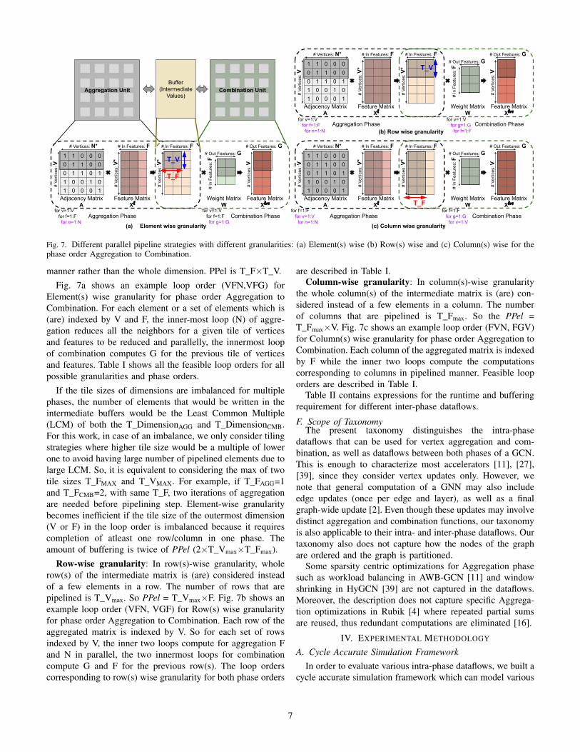
Fig. 7. Different parallel pipeline strategies with different granularities: (a) Element(s) wise (b) Row(s) wise and (c) Column(s) wise for thephase order Aggregation to Combination.
manner rather than the whole dimension. PPel is T_F×T_V.
Fig. 7a shows an example loop order (VFN,VFG) forElement(s) wise granularity for phase order Aggregation toCombination. For each element or a set of elements which is(are) indexed by V and F, the inner-most loop (N) of aggre-gation reduces all the neighbors for a given tile of verticesand features to be reduced and parallelly, the innermost loopof combination computes G for the previous tile of verticesand features. Table I shows all the feasible loop orders for allpossible granularities and phase orders.
If the tile sizes of dimensions are imbalanced for multiplephases, the number of elements that would be written in theintermediate buffers would be the Least Common Multiple(LCM) of both the T_DimensionAGG and T_DimensionCMB.For this work, in case of an imbalance, we only consider tilingstrategies where higher tile size would be a multiple of lowerone to avoid having large number of pipelined elements due tolarge LCM. So, it is equivalent to considering the max of twotile sizes T_FMAX and T_VMAX. For example, if T_FAGG=1and T_FCMB=2, with same T_F, two iterations of aggregationare needed before pipelining step. Element-wise granularitybecomes inefficient if the tile size of the outermost dimension(V or F) in the loop order is imbalanced because it requirescompletion of atleast one row/column in one phase. Theamount of buffering is twice of PPel (2×T_Vmax×T_Fmax).
Row-wise granularity: In row(s)-wise granularity, wholerow(s) of the intermediate matrix is (are) considered insteadof a few elements in a row. The number of rows that arepipelined is T_Vmax. So PPel = T_Vmax×F. Fig. 7b shows anexample loop order (VFN, VGF) for Row(s) wise granularityfor phase order Aggregation to Combination. Each row of theaggregated matrix is indexed by V. So for each set of rowsindexed by V, the inner two loops compute for aggregation Fand N in parallel, the two innermost loops for combinationcompute G and F for the previous row(s). The loop orderscorresponding to row(s) wise granularity for both phase orders
are described in Table I.Column-wise granularity: In column(s)-wise granularity
the whole column(s) of the intermediate matrix is (are) con-sidered instead of a few elements in a column. The numberof columns that are pipelined is T_Fmax. So the PPel =T_Fmax×V. Fig. 7c shows an example loop order (FVN, FGV)for Column(s) wise granularity for phase order Aggregation toCombination. Each column of the aggregated matrix is indexedby F while the inner two loops compute the computationscorresponding to columns in pipelined manner. Feasible looporders are described in Table I.
Table II contains expressions for the runtime and bufferingrequirement for different inter-phase dataflows.
F. Scope of TaxonomyThe present taxonomy distinguishes the intra-phase
dataflows that can be used for vertex aggregation and com-bination, as well as dataflows between both phases of a GCN.This is enough to characterize most accelerators [11], [27],[39], since they consider vertex updates only. However, wenote that general computation of a GNN may also includeedge updates (once per edge and layer), as well as a finalgraph-wide update [2]. Even though these updates may involvedistinct aggregation and combination functions, our taxonomyis also applicable to their intra- and inter-phase dataflows. Ourtaxonomy also does not capture how the nodes of the graphare ordered and the graph is partitioned.
Some sparsity centric optimizations for Aggregation phasesuch as workload balancing in AWB-GCN [11] and windowshrinking in HyGCN [39] are not captured in the dataflows.Moreover, the description does not capture specific Aggrega-tion optimizations in Rubik [4] where repeated partial sumsare reused, thus redundant computations are eliminated [16].
IV. EXPERIMENTAL METHODOLOGY
A. Cycle Accurate Simulation FrameworkIn order to evaluate various intra-phase dataflows, we built a
cycle accurate simulation framework which can model various
7

TABLE IIRUNTIME AND BUFFERING REQUIREMENTS FOR INTER-PHASE
DATAFLOWS
Inter-phase Intermediate Runtimedataflow BufferingSeq V×F tAGG+tCMBSP-arbitrary T_V×T_F tAGG+tCMBSP-EnGN-like 0 tAGG+tCMB-tloadPP-elements 2×T_Vmax×T_Fmax sum(max(tAGG,tCMB)PPel)PP-Row 2×T_Vmax×F sum(max(tAGG,tCMB)PPel)PP-Column 2×V×T_Fmax sum(max(tAGG,tCMB)PPel)
dataflows. We build our cycle accurate framework aroundSTONNE simulator [29].
STONNE simulator models flexible accelerators MAERI[24] and SIGMA [33]. The underlying hardware model con-sists of a flexible distribution network with distribution latencyof one cycle and the reduction is tree based. The simulator cansupport re-configurable spatial reduction sizes. The enginescan therefore handle different tile sizes. We add support forSpMM (Sparse×Dense) memory controller in STONNE. Thesimulator can be used in both SpMM configuration and Denseconfiguration and is used to compute the complete phasesaggregation and combination respectively. To implement inter-phase dataflows, we built an analytical model around thesimulator that computes the runtime and energy of a GNNlayer. We input the sparse graphs of the workloads using CSRformat and use the dimensions V, F and G as the inputs to theframework
In this work, since our goal is to compare the impact ofthe dataflows, we assume that there is sufficient buffering torun any dataflow to ensure that there are no stalls due todata fetches from the memory. Any performance differenceis purely due to under-utilization of a dataflow, loading andstreaming delays, and stalls in parallel pipeline dataflow.
B. Dataflow EvaluatorFor evaluation, we choose 8 representative dataflows. All
the configurations have phase order from Aggregation toCombination and vertex is always the outermost loop. Parallelpipeline dataflow assumes row-wise granularity and since thenumber of vertices is high, it is possible to have differentnumber of rows to have different impact. Sequential pipelinehas vertex as the outer loop and feature as the inner loopbecause of the huge amount of memory saving in that order.The dataflow configurations have been named based on thetaxonomy in Section III-D. Since we select a subset ofmapping choices, we use a compact dataflow name for theevaluation section. The compact name consists of three partsseparated by ’-’. First part represents Inter-phase dataflow,second part indicates dimensions which are necessarily spatialor temporal for aggregation and the third part (if any) indicatesdimensions which are necessarily spatial or temporal for com-bination. In third part of compact name for PP the subscriptscorresponding to the vertex are t/sl for lower(l) granularityand sh for higher(h) granularity. We also introduce High-Vs-SP dataflow to highlight the problem of parallelizing sparsedimensions for all datasets except proteins and Mutag where
T_V is already high due to smaller T_F limited by F. Table III1
describes all the configurations that we use for evaluations.
TABLE IIIREPRESENTATIVE DATAFLOW CONFIGURATIONS FOR EVALUATION.
Dataflow Configuration Compact DescriptionSeqAC(VxFxNt,VxGxFx) Seq-Nt Sequential dataflow
Temporal AggregationSeqAC(VxFxNs,VxGxFx) Seq-Ns Sequential dataflow
Spatial AggregationSPAC(VxFsNt,VxFsGx) SP-FsNt-Fs Sequential Pipeline dataflow
EnGN-likeTemporal AggregationRelatively high T_F
SPAC(VsFxNt,VsFxGx) SP-VsNt-Vs Sequential Pipeline dataflowEnGN-likeTemporal AggregationRelatively high T_V
PPAC(VxFxNt,VxGxFx) PP-Nt-Vt/sl Parallel Pipeline dataflowTemporal AggregationHyGCN-likeGranularity of lower rows
PPAC(VxFxNs,VxGxFx) PP-Ns-Vt/sl Parallel Pipeline dataflowSpatial AggregationGranularity of lower rows
PPAC(VxFxNt,VsGxFx) PP-Nt-Vsh Parallel Pipeline dataflowTemporal AggregationHyGCN-likeGranularity of higher rows
PPAC(VxFxNs,VsGxFx) PP-Ns-Vsh Parallel Pipeline dataflowSpatial AggregationGranularity of higher rows
SPAC(VsFxNt,VsFxGx) High-Vs-SP SP dataflow with high T_V
TABLE IVDATASETS INFORMATION. FIRST HALF FOR GRAPH CLASSIFICATION (WEUSE BATCH SIZE OF 64), BOTTOM HALF FOR NODE CLASSIFICATION. (*
MEANS THAT INDICATOR VECTORS WERE USED IN PLACE OF FEATURES).
Name # Graphs # Nodes(avg)
# Edges(avg) # Features
Mutag (MU) 188 17.93 19.79 28*Proteins (PR) 1113 39.06 72.82 1(reg)/29(full)Imdb-bin (IB) 1000 19.77 96.53 136*Reddit-bin (RB) 2000 429.63 497.75 3782*Collab (CL) 5000 74.49 2457.78 492*Citeseer (CS) 1 3327 9464 3703Cora (CR) 1 2708 10858 1433
C. GNN Algorithms and Datasets
We evaluate the dataflows described in Table III for GCN[22] for the target datasets described in Table IV. For eachdataflow, we also selected appropriate tile sizes as describedbelow to create a complete mapping.
D. Choosing Tile SizesWe pick a few representative tile sizes for our analysis,
based on the following heuristics.
• Number of PEs=512 and Mapping Efficiency (Product ofTile sizes/Number of PEs) is close to 100%. Since Parallel
1Our purpose here is to not compare HyGCN and EnGN’s underlyingimplementation. We evaluate HyGCN-like (PP) and EnGN like (SP) dataflowsto understand the factors affecting the runtime associated with the dataflows.
8

a) b)
Fig. 8. Aggregation dataflow- VtFxNx. Impact of tile size T_N onperformance for graphs with (a) V=10000 (High) and F=32 (low)and (b) F=512 (High) and V=1000 (Low) for varying average degrees(D). Number of PEs = 128. T_V=1 and T_F=128/T_N. Runtime isnormalized by runtime correspoding to highest D and lowest T_N
Pipeline has two phases operating in parallel, to have samenumber of total PEs, each phase has 256 PEs.
• For SP, we use EnGN-like dataflow. The buffer setup timebetween aggregation and combination is 0, that is theintermediate outputs are directly in PEs for next phase.T_VAgg=T_VCmb and T_FAgg=T_FCmb. T_N=1 since theintermediate matrix should be accumulated inside PE.
V. EVALUATION
A. Runtime Analysis using Synthetic Matrices
In this subsection we evaluate GCN [22] on syntheticmatrices to understand the impact of tile sizes for some ofthe dataflows in Table III. Synthetic workload used comprisesof GEMMs. Each of the synthetic adjacency matrices usedhave varying number of edges (i.e., sparsity ratio).
1) Intra-phase dataflows: Here, we evaluate the factorsthat influence the performance of an individual phase. For,combination (Dense) phase, there is a vast literature describingDense CNNs and Dense GEMMs and we refer the reader toKwon et al. [23].
For Aggregation (SpMM), two primary factors that influ-ence the run-time is the set of tile sizes for various dimensionsand the amount of sparsity. Large T_N can lead to under-utilization of PEs. However if T_N=1, latency can be highspecially when the second phase needs to use the output soon,for example PP. The impact of tile sizes on performance fordifferent graphs is shown in Fig. 8. These plots show that asthe graph becomes more densely connected, higher T_N ismore optimal. Thus, optimal tile size for reduction in SpMMdepends on the graph sparsity.
2) Inter-phase dataflows: The factors affecting the perfor-mance of Sequential dataflow are same as the factors affectingdataflows of individual phases as the number of cycles issimply the sum of number of cycles of individual phases.
In Parallel Pipeline dataflow, the delay is governed by theslower phase. Therefore intra-phase performance is critical toparallel pipeline. Parallel pipeline is also affected by gran-ularity as increase in granularity increases the delay of thenon-overlapping part. Fig. 9a shows the impact of temporalor spatial reduction in Aggregation on overall pipelining.For lower average degrees, combination delay dominates the
a) b)
Fig. 9. Impact of factors affecting pipelining for Aggregation followedby Combination. V=1024, F=512 and G=16 and number of PEs=512for each phase for different average degrees D. (a) shows the runtimefor different tile sizes. Dataflow - PPAC(VtFxNx, VtGsFs). T_N inthe inter-phase pipeline. T_V=1, T_FCMB=32, T_G=16, T_FAGG =512/T_N. (b) shows the variation of performance with the increase ingranularity of pipelining. Dataflow- PPAC(VtFsNt, VxGtFx). V=1024,T_VCMB is varied and it represents the number of rows beingpipelined. T_FCMB=512/T_VCMB.
Fig. 10. Impact of factors affecting interleaving for Aggregation fol-lowed by Combination. Dataflow - SPAC(VxFxNt,VxFxGt). V=1024,F=512, G=16, Number of PEs = 512. These figures show the impactof different tile size combinations T_V and T_F. Sequential pipeliningfor T_V = {1,8,64,512}. T_V = 512/T_V with T_N = T_G = 1. Notethat this example does not aim to model exact EnGN implementation.Here, inter-phase dataflow is EnGN like.
Aggregation and thus change in T_N does not impact thenet delay. But as average degree increases, Aggregation delaystarts to dominate and affect the net delay. Fig. 9b shows theimpact of having high granularity on performance. On increas-ing T_VCMB, the parallel pipeline delay first decreases dueto parallelization of the stationary dimension V but increasesbecause of the increase in the non-overlapping delay.
For SP, we use EnGN-like dataflow. We evaluate thisdataflow for phase order aggregation to combination for tilesizes T_F and T_V.
Fig. 10 shows the impact of different tile sizes T_V and T_Fon interleaving. In this example, aggregation and combinationhave vertex in the outermost loop. Thus, tiling T_V spatiallyreduces the number of cycles needed to load vertices in thePEs, however, beyond a point the latency becomes higher. Themain reason for that is that V is an irregular dimension andparallelizing V implies that the computation is limited by thevertex with most neighbors in the tile which is referred toas "evil row" in AWB-GCN [11]. The impact of evil row ismore significant in real world graphs. AWB-GCN has a loadbalancing engine that schedules the evil row on multiple PEs.Alternatively, one can also choose lower T_V.
9

Thus the choice of tile sizes has a huge impact on eachdataflow and the optimal tile sizes can vary with the graph.
B. Runtime Evaluation on Real Graph Structures
We evaluate dataflow configurations in Table III for datasetsin IV. Figure 11 shows the GCN runtimes normalized by thedelay of Seq-Nt dataflow. Our observations are as follows-
• For Collab, spatial reduction (Ns) in general performsmuch better than temporal reduction (Nt), since Collabis densely connected, for Imdb, the performance is similarwhich means optimal is between 1 and 10, for otherdatasets, since they are sparse, optimal T_N is low.
• SP-VsNt-Vs performs well in most of the cases sinceparallelization of the vertices leads to reduced loadingoverhead, however, as observed in most of the datasets,specially in Reddit-bin, Citeseer and Cora, extremely highT_V can lead to delay as the performance is limited bythe evil row as demonstrated in High-Vs-SP dataflow
• For PP dataflow, spatial or temporal reduction hasmore impact on runtime compared to the granularity ofpipelining. This is because pipelining delay is dominatedby the slower phase and the non-overlapping extra delayis that of a faster phase.
• For all datasets SP-FsNt-Fs and PP-Nt-Vt/sl have tilingssuch that PP-Nt-Vt/sl computes both phases in parallelwith half the feature tile size compared to SP-FsNt-Fs.Yet both SP-FsNt-Fs and PP-Nt-Vt/sl display differentcharacteristics across different workloads.
The impact of a mapping or a tile size is highly dependent onthe graph structure.
C. Energy of GNN Dataflows
This subsection discusses the on-chip energy for GNNdataflows. Fig 12 shows the Energy consumed by variousdataflows for various workloads. We assume the energy ofa global buffer (GB) access to be 1.046pJ and the energy ofa local buffer (L1) access to be 0.053pJ based on the energymodel from Dally et al. [7]. Some of the observations relatedto energy are as follows:
• Energy is dominated by GB reads followed by L1 reads.• Energy trends for T_N are similar to performance across
applications. Collab favors high T_N while most of theothers favor low T_N.
• SP usually exhibits low energy but that is not true forHigh-Vs-SP.
• Fig 13 shows the GB access breakdown for two examples,since GB energy is dominant. SP dataflow does not haveGlobal Buffer Intermediate accesses, since the secondphase uses the data locally in PE. SP dataflow has partialsum (psum) accesses because T_F features are processedat once and then phases are switched. When T_F is lowin High-Vs-SP, increase in psum accesses compensates forthe reduction in Intermediate data accesses.
• In Mutag, where the number of features is low, input fea-ture map reads in the Agg phase dominate but in Citeseerwhere the number of features is even higher than the num-ber of vertices, weight reads in the Cmb phase dominate.
• High T_VCMB reduces the Weight Read energy consider-ably due to spatial reuse of vertices in DenseGEMM.
D. Takeaways, Insights and Architectural Vision
Graph datasets have highly irregular structures which evenamongst datasets are different. We have observed in theevaluations using both synthetic and real workloads that tilesizes are critical to performance and energy. In terms of energy,SP-VsNt-Vs works well, however there is an optimal T_Vfor which the energy is the best. In terms of runtime, SPworks well for low F (but there is an optimal T_V) but PPworks well for high F (RedditBIN, Cora, Citeseer) with highT_VCMB. For runtime and energy, there is an optimal T_Vin SP dataflow. Parallelizing V dimension improves latency,however the performance can be limited by evil row if T_Vis too large. From energy perspective, high T_V reduces theweight reads but also increases the partial sum accesses (dueto low T_F) as shown in Fig 13.
The choice of desired metric influences the design choices.To achieve optimal energy, SP dataflow with flexible distri-bution network for variable T_V, T_F is a good choice. Forperformance, the optimal inter-phase dataflow is workloaddependent. For acceleration of all GNN workloads, we needa flexible accelerator substrate for GNNs with an ability tochoose various intra-phase parameters like tile sizes and alsowith the ability to model inter-phase dataflows - sequentialpipeline and parallel pipeline. Note-By "flexibility" we meanconfigurability of tile-sizes and partition sizes, not Turing-completeness like CPUs/GPUs.
Our vision for the flexible accelerator is as follows:• A flexible Network-On-Chip (NoC) for Intra-phase
dataflows which adds the ability to support reduction anddistribution of variable tile sizes for each dimension like inMAERI [24] and SIGMA [33]. This will always be helpfulwhatever the inter-phase dataflow since intra-phase metricsdepend on tile sizes.
• Supporting variable sized splitting of a substrate into twophases for parallel pipelining which requires a flexibleNoC and homogeneous substrate.
• The ability to support different inter-phase dataflows, ahigh-level architecture of which is shown in Fig. 14
• The ability to turn off intermediate buffers when notneeded for EnGN like SP dataflow to save energy.
VI. RELATED WORK
The acceleration of GNN workloads is an active area ofresearch that distinguishes between software and hardwareacceleration [2]. On the one hand, software acceleration forGNNs aims at exploiting the knowledge of the graph propertiesto better adapt the workload to the underlying hardware [4],[10], [14], [16], [20], [28], [34]–[37], [45]. This includes
10

Fig. 11. Runtimes of Dataflows normalized to Seq-Nt for GCN algorithm. Tile sizes are represented as(T_VAGG,T_N,T_FAGG,T_VCMB,T_G,T_FCMB)
Fig. 12. On-Chip Buffer access energies of Dataflows, GB is Global Buffer and L1 is local (PE) buffer
Fig. 13. Global Buffer breakdown for Mutag and Citeseer, Adj-Adjacency matrix, Inp-Input matrix, Int-Intermediate matrix, Wt-weight matrixand Op-output matrix, Psum-partial sum accesses
Reduction N
etwork
Dist. N
etwork
Intermediate BufferIntermediate Buffer
Reduction N
etwork
Dist. N
etwork
Intermediate Buffer
Reduction N
etwork
Dist. N
etwork
(a) Sequential / Sequential Pipeline (b) Pipeline Parallel
Fig. 14. Supporting multiple inter-phase dataflows in an accelerator.
techniques such as intelligent partitioning [34], sparsity-awareworkload management [37], vertex reordering [4], or thecaching of partial aggregations to avoid redundant sums [16].These techniques are either specific for GPUs, such as thedataflow constructs in Neugraph [28], or orthogonal to the
dataflow approach.
On the other hand, hardware accelerators employ specificarchitectures to combat the alternating dense–sparse phasesof GNNs and to adapt to their time-varying needs [3], [4],[11], [21], [27], [39], [42]. The existing accelerators tacklethe challenge in various ways. For instance, EnGN [27] relieson a unified architecture to perform both aggregation andcombination efficiently, whereas HyGCN [39] utilizes twoseparate engines to that end. Centaur [15] tackles both denseand sparse computations, although not aiming directly atGNNs. Finally, we highlight GRIP [21] as being among thefirst accelerators to explicitly consider edge updates. Eachof these hardware accelerators inherently implements a givendataflow, but the choice is generally fixed and not formallystated. This is, to the best of our knowledge, none of thelisted works formalize the taxonomy for the dataflows for
11

GNN accelerators. Recently, GCNAX [26] proposed a flexibleaccelerator with Design Space Exploration to choose the idealdataflow for a workload. Recently, there has also been work onanalytical modelling of data movement for GNN accelerators[12].
VII. CONCLUSION
GNN accelerators are recently becoming extremely popular.Each accelerator has picked a specific dataflow to stage theGNN computations on the accelerator’s compute and memoryresources. To date, there exists no systematic mechanism toqualitatively and quantitatively compare different accelerators.This is the first work to propose a taxonomy to describethe space of dataflow choices for GNN accelerators. Thetaxonomy captures intra- and inter- phase dataflows and thenaccurately analyzes the hardware requirements and perfor-mance characteristics. We envision this work paving the wayfor systematic study and design of future GNN accelerators.
ACKNOWLEDGEMENTS
Support for this work was provided through the ARIAA co-design center funded by the U.S. Department of Energy (DOE)Office of Science, Advanced Scientific Computing Researchprogram. Sandia National Laboratories is a multimission lab-oratory managed and operated by National Technology andEngineering Solutions of Sandia, LLC., a wholly owned sub-sidiary of Honeywell International, Inc., for the U.S. Depart-ment of Energy’s National Nuclear Security Administrationunder contract DE-NA-0003525.
REFERENCES
[1] “Nvidia nsight,” in https://developer.nvidia.com/nsight-visual-studio-edition, 2018.
[2] S. Abadal, A. Jain, R. Guirado, J. López-Alonso, and E. Alarcón, “Com-puting graph neural networks: A survey from algorithms to accelerators,”arXiv preprint arXiv:2010.00130, 2020.
[3] A. Auten, M. Tomei, and R. Kumar, “Hardware Acceleration of GraphNeural Networks,” DAC, 2020.
[4] X. Chen, Y. Wang, X. Xie, X. Hu, A. Basak, L. Liang, M. Yan, L. Deng,Y. Ding, Z. Du et al., “Rubik: A hierarchical architecture for efficientgraph learning,” arXiv preprint arXiv:2009.12495, 2020.
[5] Y. Chen, T. Yang, J. Emer, and V. Sze, “Eyeriss v2: A flexible acceleratorfor emerging deep neural networks on mobile devices,” IEEE Journalon Emerging and Selected Topics in Circuits and Systems, vol. 9, no. 2,pp. 292–308, 2019.
[6] Y.-H. Chen, J. Emer, and V. Sze, “Eyeriss: A spatial architecturefor energy-efficient dataflow for convolutional neural networks,” inProceedings of the 43rd International Symposium on ComputerArchitecture, ser. ISCA ’16. IEEE Press, 2016, p. 367–379. [Online].Available: https://doi.org/10.1109/ISCA.2016.40
[7] W. J. Dally, Y. Turakhia, and S. Han, “Domain-specific hardwareaccelerators,” Commun. ACM, vol. 63, no. 7, p. 48–57, Jun. 2020.[Online]. Available: https://doi.org/10.1145/3361682
[8] D. K. Duvenaud, D. Maclaurin, J. Iparraguirre, R. Bombarell, T. Hirzel,A. Aspuru-Guzik, and R. P. Adams, “Convolutional networks on graphsfor learning molecular fingerprints,” in Advances in neural informationprocessing systems, 2015, pp. 2224–2232.
[9] W. Fan, Y. Ma, Q. Li, Y. He, E. Zhao, J. Tang, and D. Yin, “Graphneural networks for social recommendation,” in The World Wide WebConference, 2019, pp. 417–426.
[10] M. Fey and J. E. Lenssen, “Fast graph representation learning withpytorch geometric,” arXiv preprint arXiv:1903.02428, 2019.
[11] T. Geng, A. Li, T. Wang, C. Wu, Y. Li, R. Shi, A. Tumeo, S. Che,S. Reinhardt, and M. Herbordt, “Awb-gcn: A graph convolutionalnetwork accelerator with runtime workload rebalancing,” in 2020 53rdAnnual IEEE/ACM International Symposium on Microarchitecture (MI-CRO), 2020, pp. 922–936.
[12] R. Guirado, A. Jain, S. Abadal, and E. Alarcón, “Characterizing thecommunication requirements of gnn accelerators: A model-based ap-proach,” in 2021 IEEE International Symposium on Circuits and Systems(ISCAS), 2021.
[13] W. Hamilton, Z. Ying, and J. Leskovec, “Inductive representationlearning on large graphs,” in Advances in neural information processingsystems, 2017, pp. 1024–1034.
[14] Y. Hu, Z. Ye, M. Wang, J. Yu, D. Zheng, M. Li, Z. Zhang, Z. Zhang,and Y. Wang, “Featgraph: A flexible and efficient backend for graphneural network systems,” arXiv preprint arXiv:2008.11359, 2020.
[15] R. Hwang, T. Kim, Y. Kwon, and M. Rhu, “Centaur: A chiplet-based,hybrid sparse-dense accelerator for personalized recommendations,”ISCA, 2020.
[16] Z. Jia, S. Lin, R. Ying, J. You, J. Leskovec, and A. Aiken, “Redundancy-free computation graphs for graph neural networks,” KDD, 2020.
[17] J. Jiang, J. Chen, T. Gu, K.-K. R. Choo, C. Liu, M. Yu, W. Huang, andP. Mohapatra, “Anomaly detection with graph convolutional networksfor insider threat and fraud detection,” in MILCOM 2019-2019 IEEEMilitary Communications Conference (MILCOM). IEEE, 2019, pp.109–114.
[18] N. P. Jouppi, , C. Young, N. Patil, D. Patterson, G. Agrawal, R. Bajwa,S. Bates, S. Bhatia, N. Boden, A. Borchers, R. Boyle, P. l. Cantin,C. Chao, C. Clark, J. Coriell, M. Daley, M. Dau, J. Dean, B. Gelb,T. V. Ghaemmaghami, R. Gottipati, W. Gulland, R. Hagmann, C. R.Ho, D. Hogberg, J. Hu, R. Hundt, D. Hurt, J. Ibarz, A. Jaffey,A. Jaworski, A. Kaplan, H. Khaitan, D. Killebrew, A. Koch, N. Kumar,S. Lacy, J. Laudon, J. Law, D. Le, C. Leary, Z. Liu, K. Lucke,A. Lundin, G. MacKean, A. Maggiore, M. Mahony, K. Miller, R. Na-garajan, R. Narayanaswami, R. Ni, K. Nix, T. Norrie, M. Omernick,N. Penukonda, A. Phelps, J. Ross, M. Ross, A. Salek, E. Samadiani,C. Severn, G. Sizikov, M. Snelham, J. Souter, D. Steinberg, A. Swing,M. Tan, G. Thorson, B. Tian, H. Toma, E. Tuttle, V. Vasudevan, R. Wal-ter, W. Wang, E. Wilcox, and D. H. Yoon, “In-datacenter performanceanalysis of a tensor processing unit,” in Proceedings of the 44th AnnualInternational Symposium on Computer Architecture (ISCA), 2017.
[19] K. Kersting, N. M. Kriege, C. Morris, P. Mutzel, and M. Neu-mann, “Benchmark data sets for graph kernels, 2016,” URLhttp://graphkernels.cs.tu-dortmund.de, vol. 795, 2016.
[20] K. Kiningham, P. Levis, and C. Re, “GReTA: Hardware OptimizedGraph Processing for GNNs,” in Proceedings of the Workshop onResource-Constrained Machine Learning (ReCoML 2020), March 2020.
[21] K. Kiningham, C. Re, and P. Levis, “GRIP: A Graph Neural NetworkAccelerator Architecture,” pp. 1–14, 2020. [Online]. Available:http://arxiv.org/abs/2007.13828
[22] T. N. Kipf and M. Welling, “Semi-supervised classification with graphconvolutional networks,” ICLR, 2017.
[23] H. Kwon, P. Chatarasi, M. Pellauer, A. Parashar, V. Sarkar, and T. Kr-ishna, “Understanding reuse, performance, and hardware cost of dnndataflow: A data-centric approach,” in Proceedings of the 52nd AnnualIEEE/ACM International Symposium on Microarchitecture. ACM,2019, pp. 754–768.
[24] H. Kwon, A. Samajdar, and T. Krishna, “MAERI: enabling flexibledataflow mapping over dnn accelerators via programmable intercon-nects,” in Proceedings of the Twenty-Third International Conferenceon Architectural Support for Programming Languages and OperatingSystems. ACM, 2018, p. 461–475.
[25] J. Leskovec and A. Krevl, “SNAP Datasets: Stanford large networkdataset collection,” http://snap.stanford.edu/data, Jun. 2014.
[26] J. Li, A. Louri, A. Karanth, and R. Bunescu, “Gcnax: A flexible andenergy-efficient accelerator for graph convolutional neural networks,” in2021 IEEE International Symposium on High Performance ComputerArchitecture (HPCA), 2021, pp. 775–788.
[27] S. Liang, Y. Wang, C. Liu, L. He, L. Huawei, D. Xu, and X. Li, “Engn:A high-throughput and energy-efficient accelerator for large graph neuralnetworks,” IEEE Transactions on Computers, 2020.
[28] L. Ma, Z. Yang, Y. Miao, J. Xue, M. Wu, L. Zhou, and Y. Dai,“Neugraph: Parallel deep neural network computation on large graphs,”in 2019 USENIX Annual Technical Conference (USENIX ATC 19), 2019,pp. 443–458.
12

[29] F. M. Matrínez, J. L. Abellán, M. E. Acacio, and T. Krishna, “Stonne: Adetailed architectural simulator for flexible neural network accelerators,”arXiv preprint arXiv:2006.07137v1, Jun. 2020.
[30] M. Miwa and M. Bansal, “End-to-end relation extraction using lstms onsequences and tree structures,” arXiv preprint arXiv:1601.00770, 2016.
[31] A. Parashar, P. Raina, Y. S. Shao, Y. Chen, V. A. Ying, A. Mukkara,R. Venkatesan, B. Khailany, S. W. Keckler, and J. Emer, “Timeloop:A systematic approach to dnn accelerator evaluation,” in 2019 IEEEInternational Symposium on Performance Analysis of Systems andSoftware (ISPASS), 2019, pp. 304–315.
[32] X. Qi, R. Liao, J. Jia, S. Fidler, and R. Urtasun, “3d graph neuralnetworks for RGBD semantic segmentation,” in Proceedings of the IEEEInternational Conference on Computer Vision, 2017, pp. 5199–5208.
[33] E. Qin, A. Samajdar, H. Kwon, V. Nadella, S. Srinivasan, D. Das,B. Kaul, and T. Krishna, “Sigma: A sparse and irregular gemm ac-celerator with flexible interconnects for dnn training,” in 2020 IEEEInternational Symposium on High Performance Computer Architecture(HPCA), 2020, pp. 58–70.
[34] C. Tian, L. Ma, Z. Yang, and Y. Dai, “PCGCN: Partition-Centric Pro-cessing for Accelerating Graph Convolutional Network,” Proceedings ofIPDPS 2020, pp. 936–945, 2020.
[35] A. Tripathy, K. Yelick, and A. Buluc, “Reducing communication ingraph neural network training,” arXiv preprint arXiv:2005.03300, 2020.
[36] M. Wang, L. Yu, D. Zheng, Q. Gan, Y. Gai, Z. Ye, M. Li, J. Zhou,Q. Huang, C. Ma et al., “Deep graph library: Towards efficient andscalable deep learning on graphs,” arXiv preprint arXiv:1909.01315,2019.
[37] Y. Wang, B. Feng, G. Li, S. Li, L. Deng, Y. Xie, and Y. Ding,“GNNAdvisor: an efficient runtime system for gnn acceleration ongpus,” arXiv preprint arXiv:2006.06608, 2020.
[38] Z. Wu, S. Pan, F. Chen, G. Long, C. Zhang, and P. S. Yu, “A comprehen-sive survey on graph neural networks,” arXiv preprint arXiv:1901.00596,2019.
[39] M. Yan, L. Deng, X. Hu, L. Liang, Y. Feng, X. Ye, Z. Zhang, D. Fan,and Y. Xie, “HyGCN: a GCN accelerator with hybrid architecture,” in2020 IEEE International Symposium on High Performance ComputerArchitecture (HPCA), 2020, pp. 15–29.
[40] M. Yan, Z. Chen, L. Deng, X. Ye, Z. Zhang, D. Fan, and Y. Xie,“Characterizing and understanding GCNs on GPU,” IEEE ComputerArchitecture Letters, vol. 19, no. 1, pp. 22–25, 2020.
[41] W. Yan, W. Tong, and X. Zhi, “FPGAN: an FPGA accelerator for graphattention networks with software and hardware co-optimization,” IEEEAccess, vol. 8, pp. 171 608–171 620, 2020.
[42] H. Zeng and V. Prasanna, “GraphACT: Accelerating GCN training onCPU-FPGA heterogeneous platforms,” FPGA 2020 - 2020 ACM/SIGDAInternational Symposium on Field-Programmable Gate Arrays, pp. 255–265, 2020.
[43] B. Zhang, H. Zeng, and V. Prasanna, “Hardware Acceleration of LargeScale GCN Inference,” in Proceedings of the ASAP ’20, 2020, pp. 61–68.
[44] Z. Zhang, P. Cui, and W. Zhu, “Deep Learning on Graphs: A Survey,”IEEE Trans. Knowl. Data Eng., vol. 14, no. 8, pp. 1–1, 2020.
[45] R. Zhu, K. Zhao, H. Yang, W. Lin, C. Zhou, B. Ai, Y. Li, andJ. Zhou, “AliGraph: A comprehensive graph neural network platform,”Proceedings of the VLDB Endowment, vol. 12, no. 12, pp. 2094–2105,2018.
13