STOCKHOLM SCHOOL OF ECONOMICS Department of Economics 659 Degree project in economics Spring 2018

A Taylor Rule for the Euro Area?

Angelica Arnqvist (23597) and Karolina Larsdotter Nilsson (23654)

Abstract

The purpose of this paper is to examine whether the original Taylor rule can be used to describe the monetary policy set by the European Central Bank (ECB), when using aggregated inputs for inflation and output gap from the whole euro area as well as for specific regions. If the original Taylor rule is not applicable to the monetary policy of the ECB, we aim to develop a new Taylor rule equation specially adapted for the euro area and the ECB, based on their monetary policy set 1999–2016. The methodology used is to compute the interest rate implied by the original Taylor rule and regress it on the actual interest rate set by the ECB. The conclusion is that the monetary policy of the ECB does not follow the original Taylor rule. The original Taylor rule is not applicable to the monetary policy of the ECB when breaking down the euro area into different regions either. Therefore a new Taylor rule better suitable for the euro area is developed. The new formula puts more weight on the output gap than the deviation from the inflation target, as opposed to the original Taylor rule where there are equal weights on the two variables. The new Taylor rule is shown to be applicable for almost all regions in the euro area.

Keywords: Monetary policy, Taylor rule, European Central Bank, Euro area JEL: E43, E52, E58 Supervisor: Federica Romei Date submitted: 14 May 2018 Date examined: 30 May 2018 Discussants: Ludvig Holmér and Johanna Ohlin Examiner: Johanna Wallenius

1

Acknowledgements We would like to express our gratitude to our supervisor Federica Romei for her guidance and her dedication to our project. We also want to thank Örjan Sjöberg for the introductory lectures.

2

TABLEOFCONTENTS

1.INTRODUCTION.........................................................................................................................................3

2.BACKGROUND.............................................................................................................................................52.1THESTRUCTUREOFTHEECB...................................................................................................................................52.2ECB’SMONETARYPOLICY..........................................................................................................................................52.2.1Standardmonetarypolicymeasures.........................................................................................................52.2.2Thezerolowerbound.......................................................................................................................................62.2.3Non-standardmonetarypolicymeasures................................................................................................7

2.3THEEUROAREACHALLENGE.....................................................................................................................................8

3.CURRENTSTATEOFKNOWLEDGE...................................................................................................103.1THETAYLORRULE–APOLICYRULE.....................................................................................................................103.2THETAYLORRULEANDTHEECB.........................................................................................................................133.3THETAYLORRULEANDTHEEUROAREACOUNTRIES.......................................................................................14

4.RESEARCHDESIGN.................................................................................................................................164.1SPECIFICATIONOFDETAILEDRESEARCHFOCUS.................................................................................................164.2METHODOLOGY.........................................................................................................................................................174.2.1Testingforstationarityandcointegration............................................................................................174.2.2RegressingtheoriginalTaylorrateontheECBrate........................................................................174.2.3RegressingtheregionaloriginalTaylorratesontheactualECBrate.....................................184.2.4ThemodifiedTaylorequationfortheeuroarea................................................................................204.2.5RegionalregressionsontheECBrateusingthenewTaylorequation.....................................22

4.3DATA...........................................................................................................................................................................22

5.RESULTS....................................................................................................................................................225.1REGRESSIONOFTHEORIGINALTAYLORRATEONTHEECBINTERESTRATE...............................................225.2REGRESSIONOFTHEREGIONALORIGINALTAYLORINTERESTRATESONTHEECBRATE.........................245.3THENEWTAYLORREGRESSIONFORTHEEUROAREA.......................................................................................265.4REGIONALREGRESSIONSWITHTHENEWTAYLORRATESONTHEECBRATE.............................................27

6.DISCUSSION..............................................................................................................................................28

7.CONCLUSION............................................................................................................................................30

8.REFERENCES............................................................................................................................................31

APPENDIXA..................................................................................................................................................37

APPENDIXB..................................................................................................................................................39

3

1. Introduction Since the financial crisis in 2007–2008, many countries have struggled to keep the inflation at

target levels (European Central Bank, 2018d). In its endeavours to keep the inflation at 2%,

the European Central Bank (ECB) has for the past couple of years used negative deposit

facility interest rates. The negative deposit rates have spurred a discussion about whether the

ECB should adopt alternative monetary policy measures. One of the suggestions has been to

use a mechanical formula such as the Taylor rule, instead of the flexible inflation targeting

strategy currently used (Constancio, 2017). There are even those who argue that it is time for

the ECB to normalise its monetary policy, an argument based on the Taylor rule (Alcidi,

Busse and Gros, 2017). The Taylor rule was originally designed for the Federal Reserve, the

central bank in the United States, offering a formula for the Fed funds rate. Comparing the

actual Fed funds rate and the Taylor rule predictions, one can conclude that the rates align

relatively well (Jones, 2014, p. 389). The ECB has not formally adopted a similar mechanical

formula (ECB, 2018h).

However, the modern macroeconomics is clear on the fact that policy rules have significant

advantages over a monetary policy without a pre-defined contingency plan in improving

economic performance. Hence, it should be important to preserve the concept of a policy rule

even in an environment where it is practically impossible to mechanically follow the

algebraic formulas developed by economists to describe their preferred policy rules (Taylor,

1993). Therefore we find it relevant to examine whether the Taylor rule can be applied to the

euro area and the ECB or if a similar mechanical rule could be adapted for the ECB. Thus, in

this paper, we research whether the interest rate predictions, given by the Taylor rule

historically coincide with the actual ECB interest rates. If the analysis shows that the interest

rate set by the ECB follows the Taylor rule, this could provide some predictability to the

monetary policy carried out by the ECB. It would also be possible to further analyse whether

the Taylor rule could be formally adopted as a policy rule that is part of the monetary policy

strategy of the ECB.

However, the ECB differs from the Fed, since the ECB sets a monetary policy for a range of

different countries, each with different economic preconditions. The differing economic

conditions provide further challenges for the ECB when conducting their monetary policy.

Even if our results would indicate that the ECB as a whole does not follow the Taylor rule

4

when conducting its monetary policy, it might still be possible that the ECB does follow the

Taylor rule to some extent. In other words, they might consider only a few countries in the

European Union (EU) when setting interest rates. For example, either the ECB might

consider solely the bigger economies such as Germany and France or the financially

struggling countries such as Portugal, Ireland, Italy, Greece and Spain. The applicability of

the Taylor rule will therefore also be analysed with regards to different regions in the euro

area separately.

If the Taylor rule is shown not to be explanatory of the actual interest rates, an alternative

Taylor rule, specifically adapted for the euro area, will be suggested. We determine there

might be a need for such adjustment to the original Taylor rule since this original formula was

created based on the monetary policy conducted by the Fed (in particular 1987–1992)

(Taylor, 1993). If it is possible to suggest such a formula that is suitable for the euro area, this

new formula could perhaps serve as a monetary policy rule not currently in use by the ECB.

It would provide predictability and might even prevent future challenges with low inflation.

For example, in Taylor (2009), empirical evidence showed that government actions had

worsened the financial crisis by deviating from historical principles. Therefore Taylor urged

central banks to return to interest setting principles such as the Taylor rule.

The purpose of this paper is to examine whether the original Taylor rule can be used to

describe the monetary policy set by the ECB, when using aggregated inputs for inflation and

output gap from the whole euro area as well as for specific regions. If the original Taylor rule

is shown to not be applicable to the monetary policy of the ECB, we aim to develop a "new”

Taylor rule equation specially adapted for the euro area and the ECB, based on their

monetary policy setting 1999–2016 (except July 2012–June 2014). The research questions are

thus the following:

• How well does the original Taylor rule describe the actual interest rates set by the

ECB?

• Could the ECB be said to follow the original Taylor rule when using inflation and

output gap values from a specific region?

• How could the Taylor rule be adjusted to better explain the interest rate set by the

ECB from 1999–2016 (except July 2012–June 2014)?

5

The remaining parts of the paper are divided into the following. Section 2 provides a

background of the monetary policy conducted by the ECB. Section 3 gives an overview of

the current state of research. In Section 4 the research design is presented and Section 5

contains the results. In Section 6 the results are discussed and in Section 7 the conclusion is

presented.

2. Background This section gives a background to the structure and monetary policy of the ECB. This

background information aims to give a context to the subsequent analysis to facilitate the

understanding of the thesis.

2.1 The structure of the ECB The ECB is a central bank for the EU member states having the euro as their currency,

hereafter called the euro area (European Union, 2012). The Governing Council of the ECB is

the highest decision-making body and is conducting the ECB's monetary policy. The

Governing Council consists of six Executive Board members and the central bank Governors

of the euro area countries. The Executive Board members have permanent voting rights. In

addition to this, there are 15 voting rights. The five countries that have the greatest economies

and financial sectors (Germany, France, Italy, Spain and the Netherlands) share four voting

rights and the remaining countries share 11 voting rights. The voting rights rotate between the

Governors (ECB, 2014a). The ECB is independent of any political influence, whether it is

from EU institutions or national governments (European Union, 2012). One of the aims of the

ECB being independent is to ensure it acts in the best interest of the euro area as a whole

instead of favouring certain national interests (ECB, 2017).

2.2 ECB’s monetary policy

2.2.1 Standard monetary policy measures The primary objective of the ECB's monetary policy is to maintain price stability. To reach

this objective, the ECB has adopted a monetary policy strategy comprising of a quantitative

definition of price stability, and a two-pillar approach to the analysis of the risks to price

stability. The quantitative definition of price stability does, more specifically; mean keeping

6

inflation rates below, but close to 2% (ECB, 2018e). Inflation is defined as the increase in

consumer prices and is measured by an index for the EU member states, called the

Harmonized Index of Consumer Prices (HCIP) (ECB, 2018c). The two-pillar approach is the

ECB’s approach to analyse economic developments and to assess the risks to price stability.

These two pillars are economic analysis and monetary analysis. The economic analysis is

concerned with short and medium-term price developments and the factors influencing price

development. On the other hand, the monetary analysis assesses the long-run link between

money and prices (ECB, 2018e).

The main measure used to achieve this monetary policy objective is the setting of interest

rates. There are three key interest rates set by the ECB; the interest rate on the main

refinancing operations (MROs), the rate on the deposit facility and the marginal lending

facility. The deposit facility rate is fixed at a spread below the MRO rate (Coeure, 2015). In

this paper, the interest rate on the MROs will be used as it determines the bulk of liquidity to

the banking system. Hence, the MRO rate determines the price at which banks can borrow

money from the ECB, and as a consequence, it also determines at which rate the banks can

lend out to the end consumer. Thus, if the ECB wishes to stimulate the economy they lower

the MRO, which stimulates investment, which in turn increases the inflation level. This rate

can be either variable or fixed. Since the ECB began its monetary policy measures the 1

January 1999 the interest rate has mostly been fixed, however between 28 June 2000 and 9

July 2008, the interest rate was variable (ECB, 2018b). A high-interest rate makes it more

expensive to borrow money from the bank, resulting in lower investment and consumption,

which in turn keeps the price level, that is inflation, low. On the other hand, when investment

and consumption are low, the ECB can lower the interest rate to encourage more borrowing,

investment and consumption. In turn, more investment and consumption typically raises the

inflation. In order to keep inflation at a steady level, the ECB consequently needs to adjust

the interest rate on a regular basis (Jones, 2014, pp. 306–324).

2.2.2 The zero lower bound Traditionally the perception has been that interest rates cannot go below zero (or slightly

above zero). This concept is called the zero lower bound. The reasoning underlying the

assumption of the zero lower bound is that investors would never hold a fixed-income

instrument with a risk-free negative return, since holding cash (with a zero nominal return)

7

would always be the superior alternative. Likewise, central banks were expected to be

constrained by the zero lower bound when setting monetary policy rates to stimulate the

economy. Before the financial crisis, the zero lower bound had not been a topic of discussion

since the ECB had not been close to this lower bound. However, in July 2012 the ECB set the

deposit facility rate to zero and in June 2014 the ECB decided to decrease the deposit facility

rate to a negative rate of -0.10. A new negative lower bound was thus established (Lemke and

Vladu, 2017). After this first decrease, three more rate cuts followed. In September 2014 the

ECB lowered the deposit facility rate to -0.20, in December 2015 to -0.30 and in March 2016

to -0.40 percent (ECB, 2018b). While investors considered negative interest rates

inconceivable in the euro area for a long time, investors seemed to adapt their view of the

lower bound when the ECB decreased policy rates to negative levels (Lemke and Vladu,

2017). Coeure (2015) states that the lower bound should not be seen as a strict bound on

interest rates, but it is rather the combination of standard as well as non-standard monetary

policy measures that constrain the lower bound.

2.2.3 Non-standard monetary policy measures Before the financial crisis, the standard monetary policy measures fully explained the

monetary policy conducted by the ECB. However, after the financial crisis, adjusting interest

rates have been insufficient in controlling inflation and stimulating the economy, especially

when the ECB treated the zero lower bound as binding. As a consequence, the ECB has

started to set negative interest rates, as well as introduced non-standard monetary policy

measures (ECB, 2014b). One such non-standard measure is quantitative easing which was

introduced in March 2015. Quantitative easing means that the ECB buys bonds from

commercial and public banks, which increases the price of these bonds. As a result, interest

rates fall, and people are able to borrow more money. When people can borrow more they

can consume and invest more, which leads to a higher inflation level (ECB, 2018a). Thus,

quantitative easing helps with reaching the inflation target of 2% when low interest rates are

insufficient. According to Lhuissier (2016), the impact of quantitative easing results in a

monetary condition comparable to an interest rate below -3%.

The ECB has also targeted longer-term refinancing operations (TILTROs) that provide long-

term financing to credit institutions at attractive conditions to stimulate bank lending to the

real economy (ECB, 2018f). Under the TILTRO-II program, borrowing banks can borrow up

to 30% of their outstanding loans from the ECB at a lower interest rate and with a maturity of

8

four years. Usually, the amount and cost of borrowing depend on how much loans the banks

provide the real economy, and the maturity of the loans are usually within one week or three

months. By instead providing the attractive conditions for borrowing under the TILTRO-II

program, the ECB enables borrowing banks to lend money to business and consumers in the

euro area. This, in turn, stimulates the real economy. Thus the TILTROs are also non-

standard monetary policies helping the ECB to reach its main objective (ECB, 2016).

In conclusion, the ECB monetary policy is determined by the interaction of a range of

instruments including the level of interest rates, the pace of quantitative easing and other non-

standard monetary policy tools. The different tools complement each other to generate

sustainable inflation convergence (Draghi, 2017).

2.3 The euro area challenge The ECB is different from domestic banks in Europe because the ECB has to manage

countries with such differing economies. Instead, inflation and output growth differentials in

the euro area are more comparable with other large currency areas such as the United States.

The differentials in inflation and output growth may be due to differences in demographic

trends, long-term catching-up processes or on-going adjustments leading to a more efficient

allocation of resources. As long as the inflation and output growth differentials are moderate,

there is no problem for the ECB to conduct its monetary policy for the euro area. However, if

there is a persistence of inflation and growth differentials, induced by structural inefficiencies

or misaligned national policies, of individual euro area countries over a longer period it needs

to be addressed by national policy adjustments (ECB, 2011, pp. 52–53).

9

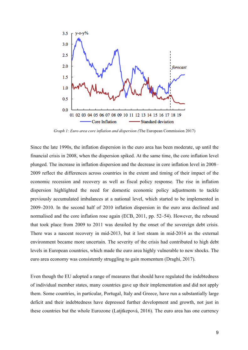
Graph 1: Euro area core inflation and dispersion (The European Commission 2017)

Since the late 1990s, the inflation dispersion in the euro area has been moderate, up until the

financial crisis in 2008, when the dispersion spiked. At the same time, the core inflation level

plunged. The increase in inflation dispersion and the decrease in core inflation level in 2008–

2009 reflect the differences across countries in the extent and timing of their impact of the

economic recession and recovery as well as fiscal policy response. The rise in inflation

dispersion highlighted the need for domestic economic policy adjustments to tackle

previously accumulated imbalances at a national level, which started to be implemented in

2009–2010. In the second half of 2010 inflation dispersion in the euro area declined and

normalised and the core inflation rose again (ECB, 2011, pp. 52–54). However, the rebound

that took place from 2009 to 2011 was derailed by the onset of the sovereign debt crisis.

There was a nascent recovery in mid-2013, but it lost steam in mid-2014 as the external

environment became more uncertain. The severity of the crisis had contributed to high debt

levels in European countries, which made the euro area highly vulnerable to new shocks. The

euro area economy was consistently struggling to gain momentum (Draghi, 2017).

Even though the EU adopted a range of measures that should have regulated the indebtedness

of individual member states, many countries gave up their implementation and did not apply

them. Some countries, in particular, Portugal, Italy and Greece, have run a substantially large

deficit and their indebtedness have depressed further development and growth, not just in

these countries but the whole Eurozone (Latjtkepová, 2016). The euro area has one currency

10

and one interest rate but lacks a fiscal union to stand alongside the monetary union. This

limits the ECB capabilities to stabilise the Eurozone and reduces differentials in inflation and

output growth across countries as they cannot recycle taxes raised in those parts of the

Eurozone that recovered well into higher spending for those parts of the Eurozone that are

performing poorly (Elliott, 2015). Apergis and Cooray (2014) point out that neither for the

EU nor the Eurozone itself is there one single recommendation for crisis measures. Instead,

they recommend that each country proceed in accordance with its specific conditions.

However, in recent years the euro area recovery has evolved from being fragile and uneven

into a firming, broad-based upswing. According to Mario Draghi (2017), there are only two

"exogenous" factors that can realistically explain the resilience of the recovery: the collapse

in oil prices in 2014–2015 and the ECB monetary policy. But even though there have been

signs of progress such as growth and employment rates converging upwards across the euro

area, significant gaps remain in terms of levels, reflecting the ECB challenge of managing

such differing economies and their inability to use fiscal policy. In large parts of the euro

area, there are still substantial under-utilised resources, reflected in a negative output gap and

high unemployment rates (Draghi, 2017).

3. Current State of Knowledge This section gives an overview of previous research conducted in the area relating to our

research questions. The original Taylor rule is presented followed by previous research

concerning the Taylor rule in relation to the ECB and to the countries in the euro area.

3.1 The Taylor rule – a policy rule In Taylor (1993), John B. Taylor examines how econometric policy evaluation research on

monetary policy rules can be applied in a practical policy-making environment. According to

this paper, which is based on Taylor’s research, a good policy rule typically calls for changes

in the federal funds rate in response to changes in the price level or changes in real income. A

policy rule is here defined as “a contingency plan that lasts forever unless there is an explicit

cancellation clause”. The opposite of a policy rule is pure discretion, where the setting for the

instruments of policy is determined from scratch each period without attempting to follow a

predefined contingency plan. As previously mentioned in the introduction, most

11

macroeconomists argue that policy rules have major advantages over discretion in improving

economic performance (Taylor, 1993).

Taylor’s research has resulted in one of the most well-known instrument rules to determine

the nominal short-term interest rate. Taylor finds that it is preferable for a country to set

interest rates based on their own economic conditions, and to pay little attention to exchange

rates (which preferably should be flexible). Also, placing a positive weight on the real output

and price-level is preferable in most countries. However, there is no consensus on the size of

the coefficients (Taylor, 1993). The rule he suggests describes how the nominal short-term

interest rate responds to inflation and the short-run output gap. The policy rule, which

captures the result of his research, is stated below.

The Taylor rule equation: 𝑖! = 𝑟 + 𝜋! + 𝑚 𝜋! − 𝜋 + 𝑛𝑌!

Where 𝑚 = 𝑛 = 0.5 (Taylor, 1993)

In the equation above 𝑖! is the nominal interest rate set at time t, 𝜋! is the inflation at time t

and 𝑌! is the GDP output gap at time t. The inflation target is 𝜋 and the real interest rate

target is 𝑟 (Jones, 2014, p. 359). The 2% equilibrium real rate is close to the assumed steady-

state growth of 2.2% (Taylor, 1993). The policy rule has the feature that the federal funds rate

raises if inflation rises above the target of 2% and decreases if it is below target. A positive

output gap results in an increase in the Fed funds rate and a negative output gap results in a

decrease. The rule was found to describe the monetary policy setting for the early years of

Alan Greenspan’s chairmanship of the Board of Governors of the U.S Federal Reserve

system “the Fed” (1987–1992) extremely well (Carare and Tchaidze, 2005).

12

Graph 2: Federal funds rate and the Taylor rate 1987–1992 (Taylor, 1993)

Although the Taylor rule is widely recognised, there is research criticising the rule.

Österholm (2003) investigates the econometric properties of the Taylor (1993) rule applied to

U.S., Australian and Swedish central banks to evaluate its empirical relevance. He concludes

that little attention has been paid to the time series properties of the data that underlie the

calculations when using interest rate rules. Using unit root tests, he shows that the variables

in the Taylor rule are likely to be integrated of order one or near integrated. Given this,

Österholm argues, that cointegration should be a necessary condition for consistent

estimation of the parameters in the model. Since this condition cannot be shown to be

satisfied, Österholm concludes that the Taylor rule generally cannot be a reasonable

description of how monetary policy is conducted. Gerlach-Kristen (2003) argues that

previous work has disregarded the factor of non-stationarity of variables when computing the

Taylor rule on the euro area. In this paper, Gerlach-Kristen estimates interest rate reaction

functions under the hypothesis that the variables of the Taylor rule have a unit root. In order

to account for the non-stationarity, a cointegration approach is taken. The results show that

the interest rate reaction functions using the cointegration approach are, in contrast to

traditional Taylor rules, stable in sample and forecast better out of sample. Based on this

research we will in this paper also test for unit roots and cointegration.

There are those who argue that the Taylor rule should not be followed strictly but rather as a

guidepost. Carlstrom and Fuerst (2003) suggest that the exact form of the Taylor rule

probably is not that important but instead that monetary policy rules should satisfy the Taylor

principle. The Taylor principle says that the nominal interest rate must increase more than for

13

each unit of increase in inflation. Such a monetary policy rule, they argue, can be used as a

guidepost for monetary policy conducted by central banks. Guideposts provide the credibility

of strict rules but make it possible to deviate from the principle to respond to unforeseen

events temporarily. This idea of having a Taylor rule as a guidepost rather than, as a strict

rule is further elaborated on in Section 6 of this paper.

3.2 The Taylor rule and the ECB Much research has been carried out regarding the Taylor rule in relation to the Fed. However,

there is also some previous research relating the Taylor rule to the ECB. Sauer and Sturm

(2003) research how Taylor rules can be used to understand the ECB monetary policy. They

begin by concluding that a form of the Taylor rule does apply to the ECB based on the ECB's

two-pillar approach. Taylor rules are thus determined applicable and their results show that

the ECB has put a higher weight on the output gap relative to inflation. These results by

Sauer and Sturm confirm the conclusion drawn by Faust et al. (2001) who argue that the ECB

has put a too high weight on the output gap relative to the inflation when they compare the

monetary policy of the ECB and the Bundesbank (the central bank of Germany). These

research papers are examples of papers where Taylor rules are determined applicable to the

monetary policy conducted by the ECB. However, these research papers do not claim that the

ECB follows the standard formula where equal weights of 0,5 are put on the inflation and the

output gap respectively. This is because the notion of “Taylor rules” here merely is defined as

a mechanical formula where the nominal interest rate is related to the output gap and the

deviation from the inflation target.

Belke and Pelleit (2006) further analyse the weights put on the deviation from the inflation

target and the output gap respectively and conclude that Taylor rules generally describe the

Fed's policy better than the ECB's policy. In this study, the monetary policies of the ECB and

the Fed are measured in the period 1999 to 2005. The results for the ECB show that the

weight on the deviation from the inflation target is smaller than the weight on the output gap

as opposed to the equal weights postulated by the original Taylor rule. Moreover, the ECB

appears to have considered money growth as an important factor in the monetary policy

strategy. The estimation results for the Fed, however, show that the weights on the deviation

from the inflation target and the output gap respectively are not too different. The authors

conclude that both the ECB and the Fed seem to follow some form of Taylor rule, but the

14

standard Taylor rule appears to describe the behaviour much better for the Fed. However, the

inflation in the euro area was low during the sample period, which they mean, might explain

why the ECB assigned such a low weight to inflation.

In conclusion, there are research papers showing that the ECB is following some kind of

Taylor rule although not the original standard formula from 1993. However, these research

papers were produced many years ago, which means there were only a few years of ECB

monetary policy included in the samples studied. Furthermore, these papers were produced

before the financial crisis, which means they are not descriptive for the more recent years.

This is because the ECB, after the financial crisis, has faced challenges previously not

encountered. Therefore we see the need for a more recent study in this area, which our

research paper is aiming to provide.

3.3 The Taylor rule and the euro area countries Our second research question is aiming to answer the question of whether the ECB can be

said to follow the Taylor rule when dividing the euro area into different regions. There is no

previous research on this exact research question. However, there are papers analysing the

monetary policy of the ECB in relation to the specific countries constituting the euro area.

Ullrich (2006) aims to answer the question of how much the economic situation of the

member states influences the interest rate decision of the council. The background to this

research question is the following. In the Statute of the ECB, the monetary policy decisions

shall be made given the situation of the euro area as a whole. However, the decision-making

body of the ECB (the Governing Council) consists of representatives of national central

banks. These representatives might consider the national economic situations over the euro

area as a whole. To investigate this question, the researcher estimates Taylor type functions

for the period 1999 to 2005 where country-specific variables for the Eurozone member states

are included. These variables include inflation rates as well as economic sentiment indicators.

The result from this research paper is that a dominant influence from specific countries

cannot be detected; meaning the decisions of the ECB do indeed take the whole euro area into

account.

However, there are research papers showing that there are notable differences in how the

single monetary policy affects each member country. Sturm and Wollmershäuser (2008)

15

analyse this issue by using Taylor rule functions. They show that the degree of adequacy of

the monetary policy of the ECB for each member country depends on the underlying

weighting scheme in the decision process. By attaching the actual policy weights that the

ECB has implicitly attached to each member country, they show that developments in small

member countries have received more than proportional weights in actual monetary policy

decisions of the ECB. Their reasoning concerns stress levels, defined as the difference

between the ECB main refinancing rate and the optimal monetary policy of a country. From a

country perspective, their results show for example that the interest rates should have been

2.8 percentage points higher in Ireland on average whereas they should have been 0.6

percentage points lower in Germany. Moons and van Poeck (2007) reach similar results in

their research paper where they aim to show whether the interest rate setting of the ECB is in

accordance with the needs of the individual member countries. In this paper, they assume that

the standard Taylor equation is applicable to the ECB’s monetary policy. Their result shows

that the ECB’s interest rate setting does not suit all European Monetary Union (EMU)

members equally well. For example, the interest rate is too high for Germany and too low for

Ireland. In a research paper by Hayo (2006) the question is whether interest rates would have

been different for the EMU countries if their national central banks had not given up control

over monetary policy to the ECB. The study period is from the year 1999 to 2004, and the

estimates of the monetary policy reaction functions are derived using Taylor rules. The

results are that most countries would have set higher national interest rates than the ECB

interest rates. The country gaining higher credibility when becoming a member of the ECB

can explain these lower interest rates. The only exception is Germany that would have set

lower national interest rates than the ECB interest rates.

In conclusion, there are research papers relating Taylor rules to the specific countries in the

euro area. However, there are no research papers that research the Taylor rule’s applicability

to regions, rather than countries. Furthermore, the results from previous papers are

contradictory, which confirms the need for more research and clarity in this area, which our

thesis is aiming to provide.

16

4. Research Design In this section we present the research design, which constitutes of the specification of our

detailed research focus, the methodology and the data sources used.

4.1 Specification of detailed research focus In order to keep the research topic focused, a number of specifications to the research

questions are made. We analyse the time period from January 1999 until December 2016,

excluding the period July 2012–June 2014. We want as large of a sample as possible to be

able to draw relevant conclusions and therefore we decide to use all the data available.

January 1999 is when the ECB introduced their monetary policy measures and after

December 2016 we lack the necessary data for the output gap. The reason we exclude the

years July 2012–June 2014 is that before July 2012 the zero lower bound was, as mentioned,

for the most part, seen as a purely theoretical problem whereas between July 2012 and June

2014 the zero lower bound became a concrete problem as further actions were required to

stimulate the economy. The Taylor formula would not have been applicable in the presence

of a zero lower bound. This is because, during the years with the zero lower bound, the ECB

would not set an interest rate below 0% even though the Taylor rule would recommend it.

However, after the replacement of the zero lower bound to a negative lower bound in June

2014, the lower bound does not appear to have been very binding since the lower bound has

decreased several times since mid-2014. As the ECB has relaxed the assumption of the “zero

lower bound” four times one could expect this to happen again if the ECB finds it necessary.

Therefore, the periods after June 2014 are included in the analysis.

In this thesis, we choose to focus on regional analysis as we find it more interesting than a

country-specific analysis. This is because we determine a regional analysis to be able to show

trends more clearly as it gives aggregate outputs. The EU countries analysed, comprising the

regions, are the countries having the euro as its currency and that joined the EU before the

year 1999. The reason for this is that the ECB is the central bank for the euro area. Hence it

makes sense to analyse the Eurozone. Furthermore the regional Taylor rate comparison to the

actual ECB rate would not be possible for all the years in our sample if we include member

states that joined after 1999.

17

An additional specification to the research focus is that the Taylor formula used is the

original equation presented by Taylor in 1993. The rule has undergone many modifications as

researchers have tried to make it a better fit for current monetary policy. However, in this

research paper, we only seek to investigate whether the ECB follows the original Taylor

formula (93) and thus this is the only one we will consider.

4.2 Methodology

4.2.1 Testing for stationarity and cointegration As mentioned, there are some previous research papers criticising the fact that the Taylor rule

has been used without taking time series properties of the data into account. When analysing

regressions using time series, the time series must be stationary. Time series that are not

stationary have a unit root. Therefore, we test whether the variables have a unit root or not.

The first order difference of non-stationary variables can be included in the regression

analysis under the condition that they are cointegrated. Cointegration means that the variables

have long run associations. If the variables are non-stationary but not cointegrated the

regression can be spurious with inconsistent estimated parameter vectors and diverging t- and

F-statistics. The augmented Dickey-Fuller (ADF) test is used to test for unit root and the

Johansen test is used to test for cointegration. Since the Johansen test is sensitive for the

number of lags we test for the recommended number of lags with lag-order statistics for VAR

and VEC (Sjö, 2008). The results of these tests can be seen in Appendix A.

4.2.2 Regressing the original Taylor rate on the ECB rate In order to answer the proposed research questions, we compute the nominal interest rate

implied by the Taylor rule (93) for the entire euro area. The idea is to compare and see if

these predicted rates could be used to explain the interest rates set by the ECB from 1999–

2016 (except July 2012 to June 2014). To make the predictions on the interest rates we use

panel data on all the inputs in the Taylor equation, including GDP output gap, inflation rate,

inflation target and the real interest rate target. With regards to our research question to

investigate if the original Taylor rule can be used to describe the monetary policy in the euro

area and due to limited and contradictory information on what input to use for the real interest

rate target in the euro area, the original value of 2% proposed by the Taylor rule (93) is used

as the real interest rate target in our equation. Data sources for the other inputs used can be

found in the data sources section. The rate implied by the Taylor rule is calculated for the

18

period 1 January 1999 to 31 December 2016 (except July 2012–June 2014). Quarterly

observations are used to increase the number of observations and also to make sure that we

capture all changes in the interest rate. To analyse if the Taylor rule can describe the ECB

interest rate, the implied nominal interest rates are regressed on the actual interest rate set by

the ECB.

4.2.3 Regressing the regional original Taylor rates on the actual ECB rate The procedure described in the above section is then repeated, but by using region-specific

inflation and output gap numbers. The point is to see how well the Taylor rule can describe

the ECB interest rate setting, when using values for inflation and output gap from specific

regions in the euro area, instead of using the inflation and output gap numbers for the whole

euro area.

FG BeNeLuxA PIIGS

France Belgium Portugal

Germany Netherlands Ireland

Luxembourg Italy

Austria Greece

Spain

Table 1: The regional split of the Eurozone countries that joined the EU before 1999

Splitting the countries in the Eurozone into different regions is done based on economic

similarities between countries. Countries with similar characteristics are placed into the same

“region”. There are several factors we take into consideration; how the countries performed

during and after the financial crisis, the geographic location of the countries, their inflation

development and the output gap of the countries. The regions can be found in Table 1. When

all countries from the Eurozone included in our sample are put in a region, the input data

(inflation, output gap) for all the countries within a region are aggregated. The aggregation of

the predictive values for a region is performed by weighting the input from each country

19

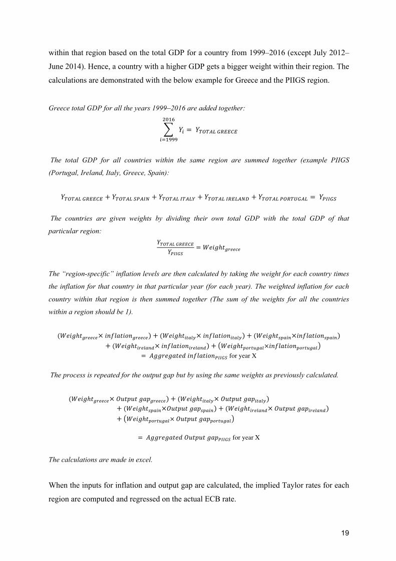
within that region based on the total GDP for a country from 1999–2016 (except July 2012–

June 2014). Hence, a country with a higher GDP gets a bigger weight within their region. The

calculations are demonstrated with the below example for Greece and the PIIGS region.

Greece total GDP for all the years 1999–2016 are added together:

𝑌!

!"#$

!!!"""

= 𝑌!"!#$ !"##$#

The total GDP for all countries within the same region are summed together (example PIIGS

(Portugal, Ireland, Italy, Greece, Spain):

𝑌!"!#$ !"##$# + 𝑌!"!#$ !"#$% + 𝑌!"!#! !"#$% + 𝑌!"!#$ !"#$%&' + 𝑌!"!#$ !"#$%&'( = 𝑌!""#$

The countries are given weights by dividing their own total GDP with the total GDP of that

particular region: 𝑌!"!#$ !"##$#

𝑌!""#$= 𝑊𝑒𝑖𝑔ℎ𝑡!"##$#

The “region-specific” inflation levels are then calculated by taking the weight for each country times

the inflation for that country in that particular year (for each year). The weighted inflation for each

country within that region is then summed together (The sum of the weights for all the countries

within a region should be 1).

(𝑊𝑒𝑖𝑔ℎ𝑡!"##$#× 𝑖𝑛𝑓𝑙𝑎𝑡𝑖𝑜𝑛!"##$#)+ (𝑊𝑒𝑖𝑔ℎ𝑡!"#$%× 𝑖𝑛𝑓𝑙𝑎𝑡𝑖𝑜𝑛!"#$%)+ (𝑊𝑒𝑖𝑔ℎ𝑡!"#$%×𝑖𝑛𝑓𝑙𝑎𝑡𝑖𝑜𝑛!"#$%)+ (𝑊𝑒𝑖𝑔ℎ𝑡!"#$%&'× 𝑖𝑛𝑓𝑙𝑎𝑡𝑖𝑜𝑛!"#$%&')+ 𝑊𝑒𝑖𝑔ℎ𝑡!"#$%&'(×𝑖𝑛𝑓𝑙𝑎𝑡𝑖𝑜𝑛!"#$%&'(

= 𝐴𝑔𝑔𝑟𝑒𝑔𝑎𝑡𝑒𝑑 𝑖𝑛𝑓𝑙𝑎𝑡𝑖𝑜𝑛!""#$ for year X The process is repeated for the output gap but by using the same weights as previously calculated.

(𝑊𝑒𝑖𝑔ℎ𝑡!"##$#× 𝑂𝑢𝑡𝑝𝑢𝑡 𝑔𝑎𝑝!"##$#)+ (𝑊𝑒𝑖𝑔ℎ𝑡!"#$%× 𝑂𝑢𝑡𝑝𝑢𝑡 𝑔𝑎𝑝!"#$%)+ (𝑊𝑒𝑖𝑔ℎ𝑡!"#$%×𝑂𝑢𝑡𝑝𝑢𝑡 𝑔𝑎𝑝!"#$%)+ (𝑊𝑒𝑖𝑔ℎ𝑡!"#$%&'× 𝑂𝑢𝑡𝑝𝑢𝑡 𝑔𝑎𝑝!"#$%&')+ 𝑊𝑒𝑖𝑔ℎ𝑡!"#$%&'(× 𝑂𝑢𝑡𝑝𝑢𝑡 𝑔𝑎𝑝!"#$%&'(

= 𝐴𝑔𝑔𝑟𝑒𝑔𝑎𝑡𝑒𝑑 𝑂𝑢𝑡𝑝𝑢𝑡 𝑔𝑎𝑝!""#$ for year X

The calculations are made in excel.

When the inputs for inflation and output gap are calculated, the implied Taylor rates for each

region are computed and regressed on the actual ECB rate.

20

4.2.4 The modified Taylor equation for the euro area In order to answer the third research question “How could the Taylor rule be adjusted to

better explain the interest rates set by the ECB from 1999–2016 (except July 2012–June

2014)?” we develop our own regression by using the inputs from the original Taylor equation

as our independent variables and the actual interest rate set by the ECB as our dependent

variable. However, due to multicollinearity between variables, we cannot include both the

inflation variable and the deviation from the inflation target variable. Multicollinearity refers

to when there is a perfect relationship between two independent variables. Hence one

independent variable could be described as a linear combination of another independent

variable. As a result when regressing all the variables from the Taylor equation on the ECB

interest rate the deviation from the inflation target automatically becomes omitted

(Wooldridge, 2012, p. 95). Therefore we choose to only keep the deviation from the inflation

target as a variable, as it is the deviation from the target that determines the ECB monetary

policy setting (ECB, 2018g). Furthermore, the real interest rate target variable is uncertain

and not possible to observe directly (Taylor, 1999) and therefore we decide to instead include

it as part of the intercept of the model. Since the relationship between the variables in the

original Taylor equation is linear, we choose to use a linear multiple regression as a starting

point. However, before performing the regression, we need to conduct a series of tests on our

data to ensure that the linear regression is, in fact, an appropriate regression model. We use

Stata to check how well our data meet the assumptions of a multiple regression (Laerd

Statistics, 2018). These conducted pre-tests can be found in the Appendix B. The following

assumptions are considered and tested for:

1) Dependent and independent variables are measured at a continuous level: The variables

have to be continuous for both the predictors and the response, which is true for our dataset

(Laerd Statistics, 2018).

2) Linearity and no significant outliers: The relationship between the predictor variables and

the outcome should be linear and there should be no significant outliers. To examine the

linear relationship between the predictors and the outcome, scatter plot diagrams are used.

Each independent variable is regressed on the dependent variable and a fitted line is added to

easier spot potential outliers in the data (Laerd Statistics, 2018).

21

3) Independence of observations: No serial correlation on data (Laerd Statistics, 2018). The

Breusch-Godfrey test is used to test for serial correlation (independence of variables). There

are two main reasons we choose Breusch-Godfrey, rather than the classical Durbin-Watson

statistic. First, the classical Durbin-Watson test relies heavily on the assumption of normally

distributed residuals, while the Breusch-Godfrey test is less sensitive to that assumption.

Second, the Breusch-Godfrey allows us to test for serial correlation through a number of lags,

as opposed to just one lag as in the Durbin-Watson test (Wooldridge, 2012, p. 422).

4) Homoskedasticity: The error variance should be constant. We begin to test the

homoscedasticity assumption using the Breusch-Pagan test. The idea behind this test is to

regress the squared residuals (e2) from the original model on all of the explanatory variables

(statadiff and outputgap), and test for the overall significance on this second regression. If

there is joint significance we conclude that the explanatory variables have an effect on the

variance of the error term and therefore there is heteroskedasticity. The null hypothesis is that

there is no joint significance (and homoskedasticity) (Wooldridge, 2012, p. 477). We also

conduct two versions of the White test. The White test is different from the Breusch-Pagan

test since it also allows for the independent variables to have a non-linear and interactive

effect on the error variance (Williams, 2015).

5) No multicollinearity: The two independent variables are not allowed to be perfectly

correlated. A VIF test is used to test for multicollinearity (Laerd Statistics, 2018).

6) Normally distributed errors: Residuals of the regression should follow a normal

distribution. To test the assumption of normally distributed errors in our regressions, we plot

a histogram of the residuals as well as conduct a Jarque-Bera test. The Jarque-Bera test has a

null hypothesis of a normal distribution, so if the null hypothesis can be rejected, then the

errors are not normally distributed (Ciuiu, 2008).

After having considered and tested for all the assumptions that must hold for unbiased

multiple regression, the ECB rate is regressed on the deviation from the inflation target and

the output gap.

22

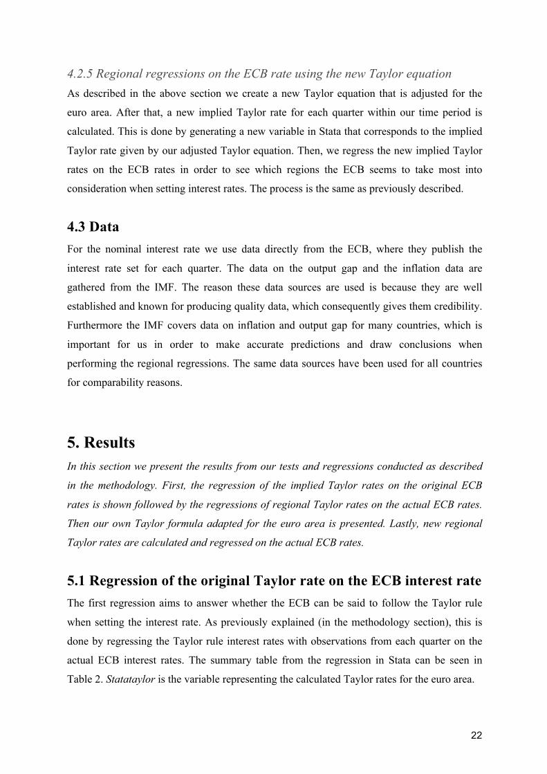
4.2.5 Regional regressions on the ECB rate using the new Taylor equation As described in the above section we create a new Taylor equation that is adjusted for the

euro area. After that, a new implied Taylor rate for each quarter within our time period is

calculated. This is done by generating a new variable in Stata that corresponds to the implied

Taylor rate given by our adjusted Taylor equation. Then, we regress the new implied Taylor

rates on the ECB rates in order to see which regions the ECB seems to take most into

consideration when setting interest rates. The process is the same as previously described.

4.3 Data For the nominal interest rate we use data directly from the ECB, where they publish the

interest rate set for each quarter. The data on the output gap and the inflation data are

gathered from the IMF. The reason these data sources are used is because they are well

established and known for producing quality data, which consequently gives them credibility.

Furthermore the IMF covers data on inflation and output gap for many countries, which is

important for us in order to make accurate predictions and draw conclusions when

performing the regional regressions. The same data sources have been used for all countries

for comparability reasons.

5. Results In this section we present the results from our tests and regressions conducted as described

in the methodology. First, the regression of the implied Taylor rates on the original ECB

rates is shown followed by the regressions of regional Taylor rates on the actual ECB rates.

Then our own Taylor formula adapted for the euro area is presented. Lastly, new regional

Taylor rates are calculated and regressed on the actual ECB rates.

5.1 Regression of the original Taylor rate on the ECB interest rate The first regression aims to answer whether the ECB can be said to follow the Taylor rule

when setting the interest rate. As previously explained (in the methodology section), this is

done by regressing the Taylor rule interest rates with observations from each quarter on the

actual ECB interest rates. The summary table from the regression in Stata can be seen in

Table 2. Statataylor is the variable representing the calculated Taylor rates for the euro area.

23

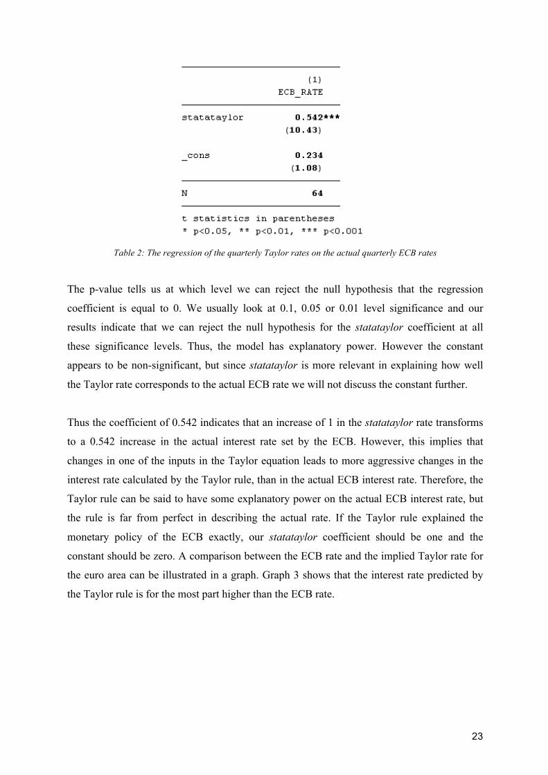
Table 2: The regression of the quarterly Taylor rates on the actual quarterly ECB rates

The p-value tells us at which level we can reject the null hypothesis that the regression

coefficient is equal to 0. We usually look at 0.1, 0.05 or 0.01 level significance and our

results indicate that we can reject the null hypothesis for the statataylor coefficient at all

these significance levels. Thus, the model has explanatory power. However the constant

appears to be non-significant, but since statataylor is more relevant in explaining how well

the Taylor rate corresponds to the actual ECB rate we will not discuss the constant further.

Thus the coefficient of 0.542 indicates that an increase of 1 in the statataylor rate transforms

to a 0.542 increase in the actual interest rate set by the ECB. However, this implies that

changes in one of the inputs in the Taylor equation leads to more aggressive changes in the

interest rate calculated by the Taylor rule, than in the actual ECB interest rate. Therefore, the

Taylor rule can be said to have some explanatory power on the actual ECB interest rate, but

the rule is far from perfect in describing the actual rate. If the Taylor rule explained the

monetary policy of the ECB exactly, our statataylor coefficient should be one and the

constant should be zero. A comparison between the ECB rate and the implied Taylor rate for

the euro area can be illustrated in a graph. Graph 3 shows that the interest rate predicted by

the Taylor rule is for the most part higher than the ECB rate.

24

Graph 3: Comparison between the actual interest rates set by the ECB and the interest rates implied by the

Taylor rule

5.2 Regression of the regional original Taylor interest rates on the ECB rate As a second step, the Taylor rates are computed for each region using regional inflation and

output gap numbers. The calculated Taylor interest rate for the different regions are then

regressed on the actual ECB interest rates. The results for all of these regressions are

demonstrated in the below table. All coefficients appear to be significant, which demonstrates

that they all have explanatory power for describing the ECB rate. As before, a coefficient

close to one indicates that the regional Taylor rate is in line with the actual ECB rate.

25

Table 3: The regressions of the quarterly regional Taylor rates on the actual quarterly ECB rates

The regional regressions (Table 3) provide similar results as the regression for the whole euro

area, except for the PIIGS Taylor coefficient, which is significantly lower. The coefficient for

the variable Taylor rate with inputs from BeNeLuxA and the coefficient for Taylor rate with

inputs from FG are both slightly higher than the Taylor coefficient with inputs from the

whole euro area and are thus more in line with the original Taylor rate. However, the

difference is marginal. For the PIIGS countries the coefficient was significantly lower

(0.374). These are the countries in the euro area that struggled the most after the financial

crisis (2008–2009) as they have suffered from poor inflation numbers and periodically

negative output gaps (IMF, 2018).

From these regressions, we conclude that it doesn’t seem like the ECB follows the original

Taylor rule when setting their interest rates. Even when computing Taylor rates using inputs

from specific regions the ECB does not seem to follow the original rule. Furthermore, since

the ECB does not appear to follow the original Taylor rule, it is not possible for us to draw

any conclusions regarding how well the different regional regressions correspond to the

actual ECB rates at this stage.

26

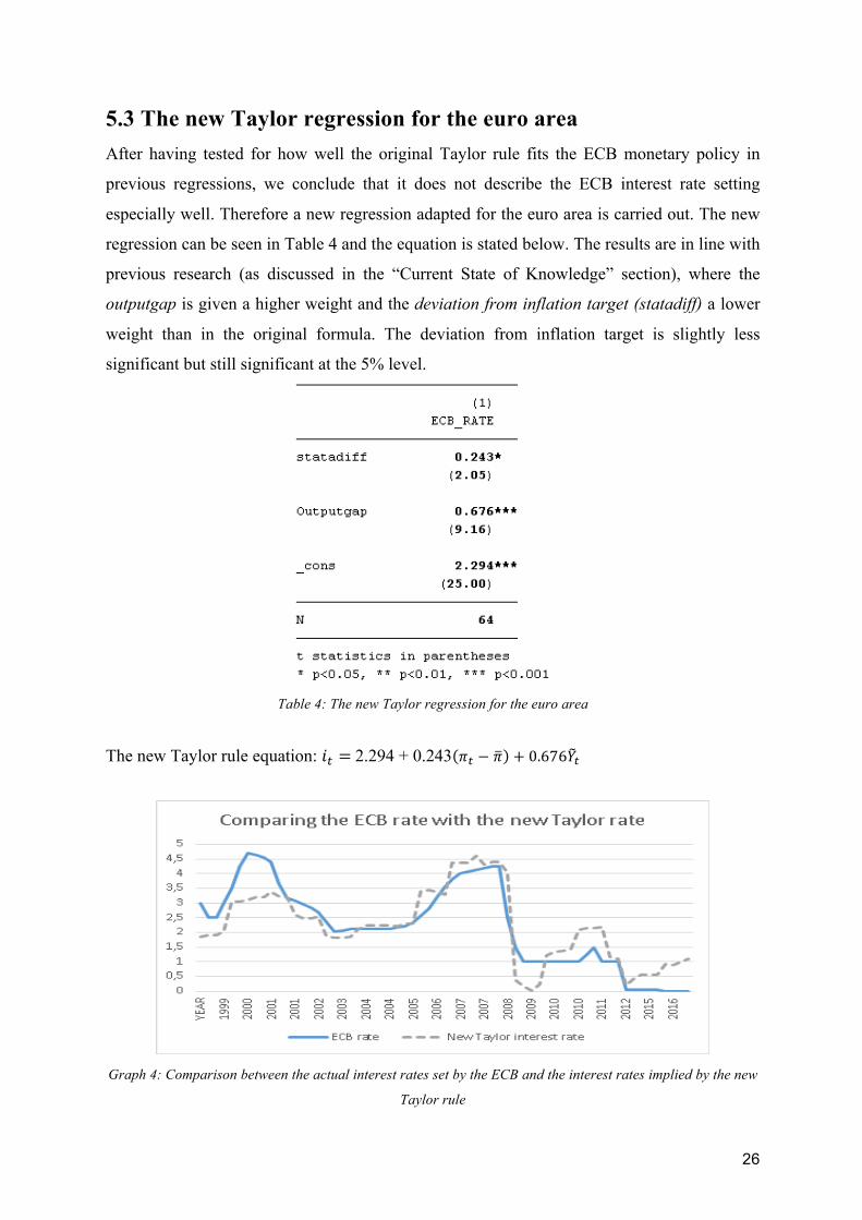
5.3 The new Taylor regression for the euro area After having tested for how well the original Taylor rule fits the ECB monetary policy in

previous regressions, we conclude that it does not describe the ECB interest rate setting

especially well. Therefore a new regression adapted for the euro area is carried out. The new

regression can be seen in Table 4 and the equation is stated below. The results are in line with

previous research (as discussed in the “Current State of Knowledge” section), where the

outputgap is given a higher weight and the deviation from inflation target (statadiff) a lower

weight than in the original formula. The deviation from inflation target is slightly less

significant but still significant at the 5% level.

Table 4: The new Taylor regression for the euro area

The new Taylor rule equation: 𝑖! = 2.294 + 0.243 𝜋! − 𝜋 + 0.676𝑌!

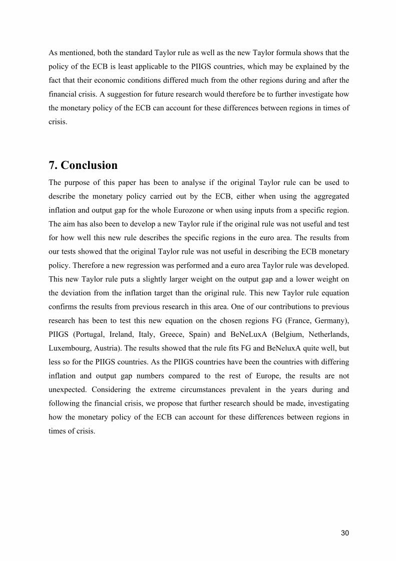
Graph 4: Comparison between the actual interest rates set by the ECB and the interest rates implied by the new

Taylor rule

27

5.4 Regional regressions with the new Taylor rates on the ECB rate The implied Taylor rates for each region are calculated again but this time by using the new

Taylor equation adapted for the euro area. The new regional Taylor rates are regressed on the

actual ECB rates. The results can be seen in the below table.

Table 5: The regression of the quarterly regional new Taylor rates on the actual quarterly ECB rates

The BeNeLuxA coefficient is the one that corresponds the best to the actual ECB rate when

comparing across all regions. The coefficient of 1.015 is very close to 1, which means that

the new regression is almost perfectly applicable to these countries’ economies. For FG the

coefficient is also close to 1. Thus the new Taylor formula is also well suited for their

economic situations. However, the coefficient of 0.465 for the PIIGS countries is the one that

corresponds the worst to the euro area coefficient of 1. As mentioned, these are the countries

that were worst affected by the financial crisis. Even though there are some correlation

between the new Taylor rates and the ECB rates, they have not been able to lower the interest

rates as much as the new Taylor rule would require. Thus, it is not unexpected that the PIIGS

Taylor rates are not in line with the actual ECB rates.

28

From this section, we conclude that the implied Taylor rates from the new equation give a

correlation closer to 1 between the regional Taylor rates and the actual ECB rates than the

original Taylor rule rates did. The new Taylor equation is thus better suited for the ECB

overall than the original Taylor equation is. Furthermore, the results seem to match fairly well

for all different regions (except for the PIIGS region for reasons mentioned), meaning that the

ECB considers all regions in the euro area when conducting their monetary policy.

6. Discussion This section presents a discussion of the results obtained above. We discuss our results and

connect them back to the purpose and research questions of our thesis, previous research and

the current economic situation in the euro area.

As mentioned in the introduction, the purpose of this thesis is to examine whether the Taylor

rule could be applied to the euro area, either when looking at the euro area as a whole or

when comparing across different regions in the euro area. The results of our study showed

that a form of Taylor rule can be applied to the euro area, although the coefficients in the

Taylor rule regression must be adjusted to better fit the ECB monetary policy.

The new Taylor rule regression confirms the results of previous research by Faust et al.

(2001), Sauer and Sturm (2003) and Belke and Pelleit (2006), who all conclude that a larger

weight is placed on the output gap and that a smaller weight is placed on the deviation from

the inflation target. Thus, despite the fact that the ECB introduced unconventional monetary

policy tools after the financial crisis in 2008, our findings confirm that the merits on which

the ECB bases its interest rate setting have not changed significantly since before the crisis.

In other words, the ECB still places a bigger weight on the output gap and a smaller weight

on the deviation from the inflation target. Thus the conclusions drawn by authors who have

conducted previous studies remain accurate in this regard. As our findings show, the original

Taylor rule cannot be said to be particularly applicable to any of the regions in the euro area.

However, when specifying our own formula, the Taylor rates implied by our new regression

correspond best to the actual ECB rates for the France-Germany region and the BeNeLuxA

region. Perhaps the rotating voting system of the ECB can be thought to give an advantage to

the greater economies Germany, France and the Netherlands. However, Italy and Spain are

29

also among the five greater economies and the new implied Taylor rates for the PIIGS

countries correspond the least to the actual ECB rates. A possible explanation can be that the

PIIGS countries have had inflation and output gap levels that differ significantly from the

other euro area countries. Since the new Taylor regression is based on aggregate inflation and

output gap levels for the euro area, where the majority of the countries have inputs closer to

for example the BeNeLuxA countries than to the PIIGS countries, it makes sense that the

regression is less applicable to the PIIGS countries. However the conclusion we draw from

the regional regression table is that most regions have a Taylor rate coefficient close to 1 and

thus it seems like the ECB take all regions into account when setting interest rates, rather than

just focusing on the major or most troubled economies.

Following up with a normative discussion, we suggest the ECB should not follow the

standard Taylor formula. Instead, they should follow a Taylor rule specifically adapted to the

euro area. In this paper, such a formula has been presented and we argue that this formula

could be adopted as part of the monetary policy strategy of the ECB. The reason for this, as

mentioned in Taylor (1993), is because monetary policy rules have major advantages over a

monetary policy without a pre-defined contingency plan for improving economic

performance. However, we do not suggest the Taylor rule to be followed in detail, especially

not in the presence of non-standard monetary policy measures. What we do suggest though, is

that this proposed Taylor rule should be used as a guidepost for monetary policy just as

Carlstrom and Fuerst (2003) argue. Guideposts would provide the credibility of strict rules

while still making it possible to temporarily deviate from the principle to respond to

unforeseen events. If the new Taylor rule would have been part of the ECB’s monetary

policy, the ECB should have started to raise their interest rate a few years ago, which can be

seen in graph 4. Instead, the ECB did the opposite and lowered the interest rates. In addition

to this, they loosed the monetary conditions further through non-standard monetary policy

measures. Therefore, if the Taylor rule is to be used as an indication, we suggest the ECB

should start to either increase their interest rates or loosen their non-standard measures. As

mentioned earlier, Alcidi, Busse and Gros (2017) also argue based on the Taylor rule that the

ECB should start to normalise their monetary policy. However, on the press conference that

was held the 26 April 2018, the ECB announced that neither the key interest rates nor the

pace of the net asset purchasing would change at this moment (Constancio and Draghi, 2018).

30

As mentioned, both the standard Taylor rule as well as the new Taylor formula shows that the

policy of the ECB is least applicable to the PIIGS countries, which may be explained by the

fact that their economic conditions differed much from the other regions during and after the

financial crisis. A suggestion for future research would therefore be to further investigate how

the monetary policy of the ECB can account for these differences between regions in times of

crisis.

7. Conclusion The purpose of this paper has been to analyse if the original Taylor rule can be used to

describe the monetary policy carried out by the ECB, either when using the aggregated

inflation and output gap for the whole Eurozone or when using inputs from a specific region.

The aim has also been to develop a new Taylor rule if the original rule was not useful and test

for how well this new rule describes the specific regions in the euro area. The results from

our tests showed that the original Taylor rule was not useful in describing the ECB monetary

policy. Therefore a new regression was performed and a euro area Taylor rule was developed.

This new Taylor rule puts a slightly larger weight on the output gap and a lower weight on

the deviation from the inflation target than the original rule. This new Taylor rule equation

confirms the results from previous research in this area. One of our contributions to previous

research has been to test this new equation on the chosen regions FG (France, Germany),

PIIGS (Portugal, Ireland, Italy, Greece, Spain) and BeNeLuxA (Belgium, Netherlands,

Luxembourg, Austria). The results showed that the rule fits FG and BeNeluxA quite well, but

less so for the PIIGS countries. As the PIIGS countries have been the countries with differing

inflation and output gap numbers compared to the rest of Europe, the results are not

unexpected. Considering the extreme circumstances prevalent in the years during and

following the financial crisis, we propose that further research should be made, investigating

how the monetary policy of the ECB can account for these differences between regions in

times of crisis.

31

8. References Alcidi, C., Busse, M. and Gros, D. 2017. Time for the ECB to normalise its monetary policy?

Insights from the Taylor rule. CEPS commentary 8 June 2017. Centre for European Policy

Studies (CEPS). https://www.ceps.eu/publications/time-ecb-normaliseits-monetary-policy-

insights-taylor-rule (16 April 2018).

Apergis, N and Cooray, A. 2014. Convergence in sovereign debt ratios across heavily

indebted EU countries: evidence from club convergence. Applied Economics Letters, vol. 21,

no. 11, pp. 786-788.

Belke, A. and Polleit, T. 2006. How the ECB and US Fed set interest rates. Applied

Economics, vol. 39, no. 17, pp. 2197-2209.

Carare, A. and Tchaidze, R. 2005. The use and abuse of Taylor rules: how precisely can we

estimate them? IMF Working Paper No. 148, International Monetary Fund.

Carlstrom, C.T. and Fuerst, T.S. 2003. The Taylor rule: a guidepost for monetary policy?

Federal Reserve Bank of Cleveland, Economic Commentary.

https://www.clevelandfed.org/en/newsroom-and-events/publications/economic-

commentary/economic-commentary-archives/2003-economic-commentaries/ec-20030701-

the-taylor-rule-a-guidepost-for-monetary-policy.aspx (16 April 2018).

Ciuiu, D. 2008. On the Jarque-Bera normality test. Working Paper Series No. 124, Technical

University of Civil Engineering Bucharest.

Coeure, B. 2015. How binding is the zero lower bound? European Central Bank.

https://www.ecb.europa.eu/press/key/date/2015/html/sp150519.en.html (10 May 2018).

Constancio, V. 2017. The future of monetary policy frameworks. European Central Bank.

https://www.ecb.europa.eu/press/key/date/2017/html/ecb.sp170525.en.html (25 March 2018).

32

Constancio, V. and Draghi, M. 2018. Press conference 26 April 2018 introductory statement.

European Central Bank.

https://www.ecb.europa.eu/press/pressconf/2018/html/ecb.is180426.en.html (2 May 2018).

Draghi, M. 2017. Monetary policy and the economic recovery in the euro area. European

Central Bank. https://www.ecb.europa.eu/press/key/date/2017/html/sp170406.en.html (2 May

2018).

Elliott, Larry. 2015. Greece’s problems are the result of the eurozone having no fiscal policy.

The Guardian. https://www.theguardian.com/business/2015/feb/01/greece-

problemseurozone-fiscal-policy-germany (25 March 2018).

European Central Bank. 2011. The monetary policy of the European Central Bank. 3rd

edition. Frankfurt am Main: European Central Bank, pp. 52-54.

https://www.ecb.europa.eu/pub/pdf/other/monetarypolicy2011en.pdf. (25 March 2018).

European Central Bank. 2014a. Rotation of voting rights in the Governing Council.

https://www.ecb.europa.eu/explainers/tell-me-more/html/voting-rotation.en.html (5 April

2018).

European Central Bank. 2014b. The ECB’s negative interest rate.

https://www.ecb.europa.eu/explainers/tell-me-more/html/why-negative-interest-rate.en.html

(4 April 2018).

European Central Bank. 2016. What is TILTRO-II?

https://www.ecb.europa.eu/explainers/tell-me/html/tltro.en.html (4 April 2018).

European Central Bank. 2017. Why is the ECB independent?

https://www.ecb.europa.eu/explainers/tell-me-more/html/ecb_independent.en.html (5 April

2018).

European Central Bank. 2018a. How quantitative easing works.

https://www.ecb.europa.eu/explainers/show-me/html/app_infographic.en.html (26 March

2018).

33

European Central Bank. 2018b. Key ECB interest rates.

https://www.ecb.europa.eu/stats/policy_and_exchange_rates/key_ecb_interest_rates/html/ind

ex.en.html (25 March 2018).

European Central Bank. 2018c. Measuring inflation – the Harmonised Index of Consumer

Prices (HICP).

https://www.ecb.europa.eu/stats/macroeconomic_and_sectoral/hicp/html/index.en.html (25

March 2018).

European Central Bank. 2018d. Monetary policy.

http://www.ecb.europa.eu/mopo/html/index.en.html (30 March 2018).

European Central Bank. 2018e. Strategy.

https://www.ecb.europa.eu/mopo/strategy/html/index.en.html (5 April 2018).

European Central Bank. 2018f. Targeted longer-term refinancing operations (TILTROs).

http://www.ecb.europa.eu/mopo/implement/omo/tltro/html/index.en.html (30 March 2018).

European Central Bank. 2018g. The definition of price stability.

https://www.ecb.europa.eu/mopo/strategy/pricestab/html/index.en.html (30 March 2018).

European Central Bank. 2018h. The Eurosystem’s instruments.

https://www.ecb.europa.eu/mopo/implement/html/index.en.html (30 March 2018).

European Central Bank Statistics. 2018. ECB statistics.

https://www.ecb.europa.eu/stats/html/index.en.html (20 February 2018).

European Commission. 2017. European economic forecast – autumn 2017. Brussels:

European Commission, p.13. https://ec.europa.eu/info/publications/economy-

finance/european-economic-forecast-autumn-2017_en (25 March 2018).

34

European Union. 2012. Protocol (No 4) on the Statute of the European System of Central

Banks and of the European Central Bank. Official Journal of the European Union, C

326/230, art. 1 and 7.

Faust, J. et al. 2001. An empirical comparison of Bundesbank and ECB monetary policy

rules. International Finance Discussion Papers No. 705, Board of Governors of the Federal

Reserve System (U.S.).

Gerlach-Kristen. 2003. Interest rate reaction functions and the Taylor rule in the euro area.

European Central Bank Working Paper No. 248, European Central Bank.

Hayo, B. 2006. Is European monetary policy appropriate for the EMU member countries? A

counterfactual analysis. Marburg Working Papers on Economics 200610, Philipps-

Universität Marburg.

International Monetary Fund. 2018. World economic outlook database.

http://www.imf.org/external/pubs/ft/weo/2018/01/weodata/index.aspx (20 February 2018).

Jones, C.I. 2014. Macroeconomics. 3rd edition. New York: W. W. Norton and Company, pp.

306-389.

Laerd Statistics. 2018. Multiple regression analysis using Stata.

https://statistics.laerd.com/stata-tutorials/multiple-regression-using-stata.php (23 March

2018).

Lajtkepová, E. 2016. Differences and similarities in the indebtedness of EU member states

after last financial crisis. Oeconomia Copernicana, vol. 7, no. 4, p. 551.

Lemke, W. and Vladu, A.L. 2017. Below the zero lower bound: a shadow-rate term structure

model for the euro area. European Central Bank Working Paper No. 1991, European Central

Bank.

35

Lhuissier, S. 2016. Through the lenses of the natural rate of interest, European monetary

policy appears to be too loose since 2015. CEPII.

http://www.cepii.fr/blog/en/post.asp?IDcommunique=469 (16 April 2018).

Moons, C. and van Poeck, A. 2007. Does one size fit all? A Taylor-rule based analysis of

monetary policy for current and future EMU members. Applied Economics, vol. 40, no. 2, pp.

193-199.

Sauer, S. and Sturm, J. 2003. Using Taylor rules to understand ECB monetary policy.

German Economic Review, vol. 8, no. 3, pp. 375-398.

Sjö, B. 2008. Testing for unit roots and cointegration - guide. Linköping University.

https://pdfs.semanticscholar.org/7ce6/2a0c7f6dab85f264a5403bf9b99a0f20a156.pdf (20

February 2018).

Sturm, J. and Wollmershäuser, T. 2008. The stress of having a single monetary policy in

Europe. KOF Working Papers No. 08-190, KOF Swiss Economic Institute, ETH Zurich.

Taylor, J.B. 1993. Discretion versus policy rules in practice. Carnegie-Rochester Conference

Series on Public Policy 39, Stanford University.

Taylor, J.B. 1999. A historical analysis of monetary policy rules. Working Paper 6768,

National Bureau of Economic Research.

Taylor, J.B. 2009. The financial crisis and the policy responses: an empirical analysis of

what went wrong. NBER Working Paper No. 14631, National Bureau of Economic Research.

Ullrich, K. 2006. An impact of country-specific economic developments on ECB decisions.

ZEW Discussion Papers No. 06-049, Center for European Economic Research.

Williams, R. 2015. Heteroskedasticity. University of Notre Dame.

https://www3.nd.edu/~rwilliam/stats2/l25.pdf (23 March 2018).

36

Wooldridge, J.M. 2012. Introductory econometrics a modern approach. 5th edition.

SouthWestern: Cengage Learning, pp. 95-477.

Österholm, P. 2003. The Taylor rule: a spurious regression? Working Paper Series No. 20,

Uppsala University.

37

Appendix A

Tests for unit root and cointegration Before regressing the ECB interest rate to the interest rate implied by the Taylor rule, we test

for unit roots and cointegration for the variables composing the Taylor formula, as described

in the methodology section.

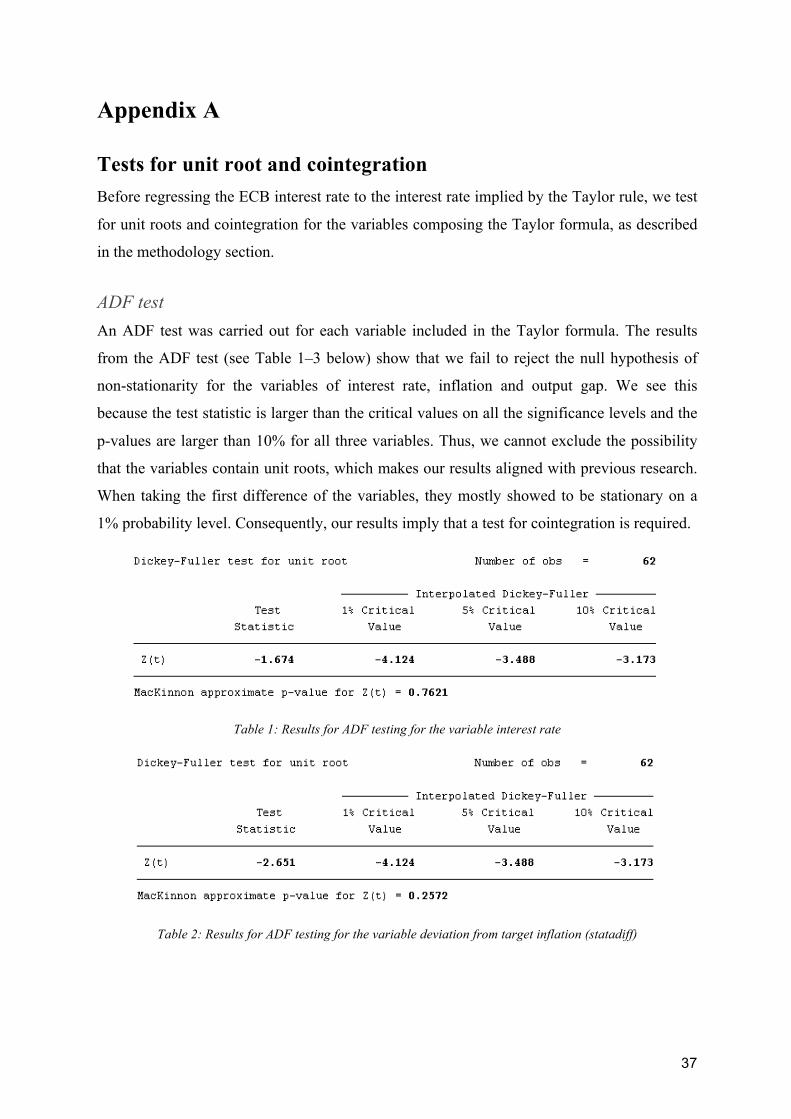
ADF test An ADF test was carried out for each variable included in the Taylor formula. The results

from the ADF test (see Table 1–3 below) show that we fail to reject the null hypothesis of

non-stationarity for the variables of interest rate, inflation and output gap. We see this

because the test statistic is larger than the critical values on all the significance levels and the

p-values are larger than 10% for all three variables. Thus, we cannot exclude the possibility

that the variables contain unit roots, which makes our results aligned with previous research.

When taking the first difference of the variables, they mostly showed to be stationary on a

1% probability level. Consequently, our results imply that a test for cointegration is required.

Table 1: Results for ADF testing for the variable interest rate

Table 2: Results for ADF testing for the variable deviation from target inflation (statadiff)

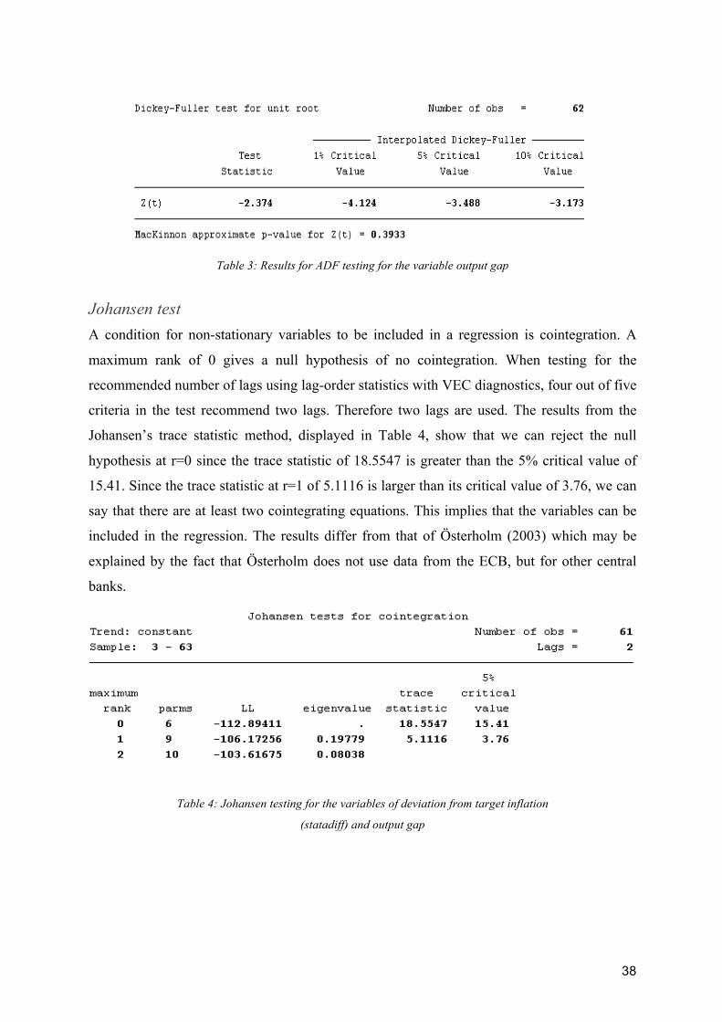
38

Table 3: Results for ADF testing for the variable output gap

Johansen test A condition for non-stationary variables to be included in a regression is cointegration. A

maximum rank of 0 gives a null hypothesis of no cointegration. When testing for the

recommended number of lags using lag-order statistics with VEC diagnostics, four out of five

criteria in the test recommend two lags. Therefore two lags are used. The results from the

Johansen’s trace statistic method, displayed in Table 4, show that we can reject the null

hypothesis at r=0 since the trace statistic of 18.5547 is greater than the 5% critical value of

15.41. Since the trace statistic at r=1 of 5.1116 is larger than its critical value of 3.76, we can

say that there are at least two cointegrating equations. This implies that the variables can be

included in the regression. The results differ from that of Österholm (2003) which may be

explained by the fact that Österholm does not use data from the ECB, but for other central

banks.

Table 4: Johansen testing for the variables of deviation from target inflation

(statadiff) and output gap

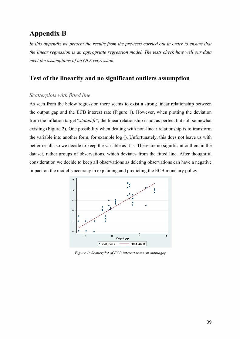
39

Appendix B In this appendix we present the results from the pre-tests carried out in order to ensure that

the linear regression is an appropriate regression model. The tests check how well our data

meet the assumptions of an OLS regression.

Test of the linearity and no significant outliers assumption

Scatterplots with fitted line As seen from the below regression there seems to exist a strong linear relationship between

the output gap and the ECB interest rate (Figure 1). However, when plotting the deviation

from the inflation target “statadiff”, the linear relationship is not as perfect but still somewhat

existing (Figure 2). One possibility when dealing with non-linear relationship is to transform

the variable into another form, for example log (). Unfortunately, this does not leave us with

better results so we decide to keep the variable as it is. There are no significant outliers in the

dataset, rather groups of observations, which deviates from the fitted line. After thoughtful

consideration we decide to keep all observations as deleting observations can have a negative

impact on the model’s accuracy in explaining and predicting the ECB monetary policy.

Figure 1: Scatterplot of ECB interest rates on outputgap

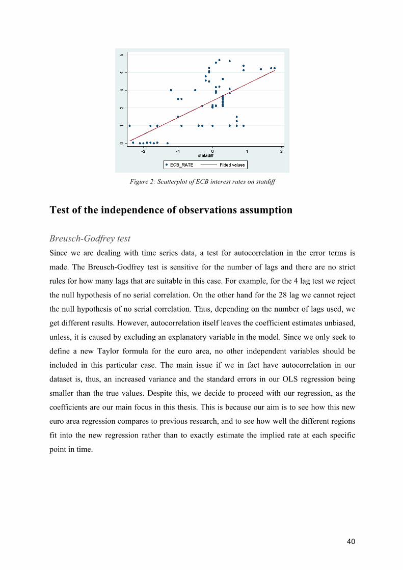
40

Figure 2: Scatterplot of ECB interest rates on statdiff

Test of the independence of observations assumption

Breusch-Godfrey test Since we are dealing with time series data, a test for autocorrelation in the error terms is

made. The Breusch-Godfrey test is sensitive for the number of lags and there are no strict

rules for how many lags that are suitable in this case. For example, for the 4 lag test we reject

the null hypothesis of no serial correlation. On the other hand for the 28 lag we cannot reject

the null hypothesis of no serial correlation. Thus, depending on the number of lags used, we

get different results. However, autocorrelation itself leaves the coefficient estimates unbiased,

unless, it is caused by excluding an explanatory variable in the model. Since we only seek to

define a new Taylor formula for the euro area, no other independent variables should be

included in this particular case. The main issue if we in fact have autocorrelation in our

dataset is, thus, an increased variance and the standard errors in our OLS regression being

smaller than the true values. Despite this, we decide to proceed with our regression, as the

coefficients are our main focus in this thesis. This is because our aim is to see how this new

euro area regression compares to previous research, and to see how well the different regions

fit into the new regression rather than to exactly estimate the implied rate at each specific

point in time.

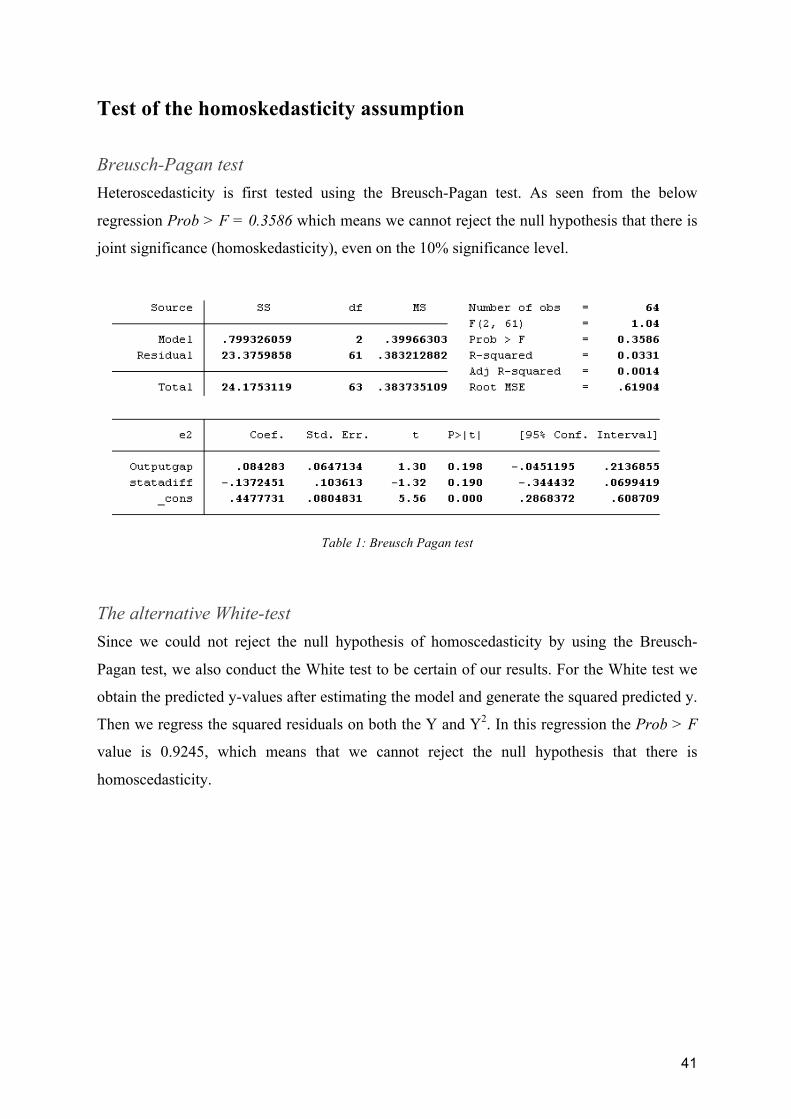
41

Test of the homoskedasticity assumption

Breusch-Pagan test Heteroscedasticity is first tested using the Breusch-Pagan test. As seen from the below

regression Prob > F = 0.3586 which means we cannot reject the null hypothesis that there is

joint significance (homoskedasticity), even on the 10% significance level.

Table 1: Breusch Pagan test

The alternative White-test Since we could not reject the null hypothesis of homoscedasticity by using the Breusch-

Pagan test, we also conduct the White test to be certain of our results. For the White test we

obtain the predicted y-values after estimating the model and generate the squared predicted y.

Then we regress the squared residuals on both the Y and Y2. In this regression the Prob > F

value is 0.9245, which means that we cannot reject the null hypothesis that there is

homoscedasticity.

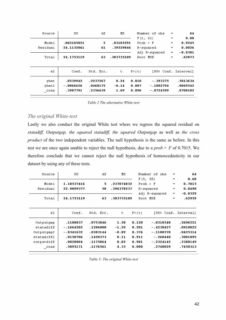
42

Table 2 The alternative White-test

The original White-test Lastly we also conduct the original White test where we regress the squared residual on

statadiff, Outputgap, the squared statadiff, the squared Outputgap as well as the cross

product of the two independent variables. The null hypothesis is the same as before. In this

test we are once again unable to reject the null hypothesis, due to a prob > F of 0.7015. We

therefore conclude that we cannot reject the null hypothesis of homoscedasticity in our

dataset by using any of these tests.

Table 3: The original White-test

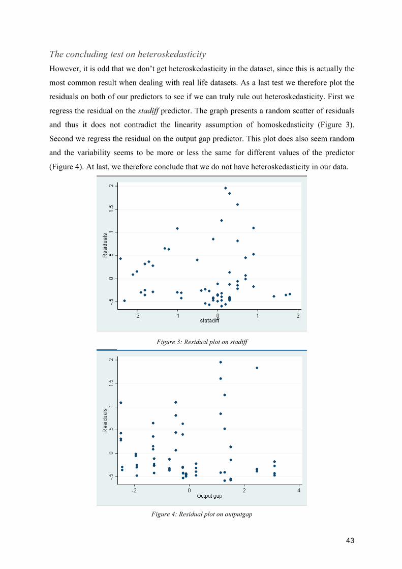
43

The concluding test on heteroskedasticity However, it is odd that we don’t get heteroskedasticity in the dataset, since this is actually the

most common result when dealing with real life datasets. As a last test we therefore plot the

residuals on both of our predictors to see if we can truly rule out heteroskedasticity. First we

regress the residual on the stadiff predictor. The graph presents a random scatter of residuals

and thus it does not contradict the linearity assumption of homoskedasticity (Figure 3).

Second we regress the residual on the output gap predictor. This plot does also seem random

and the variability seems to be more or less the same for different values of the predictor

(Figure 4). At last, we therefore conclude that we do not have heteroskedasticity in our data.

Figure 3: Residual plot on stadiff

Figure 4: Residual plot on outputgap

44

Test for multicollinearity

The VIF test To test for multicollinearity between the independent variables, the VIF test is used. If VIF is

above 5, there is a problem with multicollinearity. But as in this case VIF is below 5, which

means there is no multicollinearity between the independent variables.

Table 4: The VIF test

Test for normally distributed errors

Histogram of residuals First, we plot a histogram on the errors (residuals) of our regression. As we can see from the

below diagram the residuals seem to be normally distributed.

Figure 5: Histogram of residuals

45

Jarque-Bera test Secondly, we conduct the Jarque-Bera test, to be certain that the residuals are in fact normally

distributed in line with our assumption. As mentioned, the Jarque-Bera test has a null

hypothesis of normal distribution. As seen in Table 5 the p-value in our test is 0.5577 and

therefore we do not reject the null hypothesis. Based on the histogram and our Jarque-Bera

test we conclude that the errors are normally distributed.

Table 5: The Jarque-Bera test