A TECHNIQUE TO MEASURE CIRRUS CLOUD EFFECTIVE PARTICLE SIZE

USING A HIGH SPECTRAL RESOLUTION LIDAR

by

Ralph E. Kuehn

A thesis submitted in partial fulfillment of

the requirements for the degree of

Master of Science

(Atmospheric and Oceanic Sciences)

at the

UNIVERSITY OF WISCONSIN–MADISON

2001

Approved by:

Steven A. Ackerman

Professor, Atmospheric and Oceanic Sciences

Approved by:

Edwin W. Eloranta

Senior Scientist, Atmospheric and Oceanic Sciences

Date:

i

ACKNOWLEDGMENTS

I would like to thank my advisor Dr. Edwin Eloranta for providing me the opportunity to

work with some of the most unique and exiting lidar instruments in the world. I also appreciate

all the time he has spent teaching and guiding me through this part of my education.

My thanks also go to Professors Steve Ackerman and Greg Tripoli for their thoughtful and

constructive comments about this thesis to help improve the presentation of this work.

I would also like to thank all the present and past members of the University of Wisconsin

Lidar Group who have helped make this work possible. A special thanks go to Partrick Pon-

sardin who spent hours working with me aligning the HSRL optics, Dan Forrest for helping

me through many computer and electronic related problems with the HSRL and HSRL data

processing, and to Bob Holz for helping me collect the data used in this thesis. I also thank

Jim Hedrick for machining many new optic mounts for me and for keeping the HSRL trailer

systems in good working condition. Shane Mayor also provided a lot of help with chapter 1

and a great deal of moral support during the writing process.

Finally, I would like to thank my family for their patience and support during this part

of my education. Most importantly I would like to thank Nancy, my wife, for her love and

support, she deserves as much credit for this work as I do.

DISCARD THIS PAGE

ii

TABLE OF CONTENTS

Page

LIST OF TABLES . . . . . . . . . . . . . . . . . . . . . . . . . . . . . . . . . . . . iv

LIST OF FIGURES . . . . . . . . . . . . . . . . . . . . . . . . . . . . . . . . . . . v

ABSTRACT . . . . . . . . . . . . . . . . . . . . . . . . . . . . . . . . . . . . . . . vii

1 Introduction . . . . . . . . . . . . . . . . . . . . . . . . . . . . . . . . . . . . . 1

1.1 Motivation . . . . . . . . . . . . . . . . . . . . . . . . . . . . . . . . . . . . 11.2 Background: Lidar Instruments and the HSRL . . . . . . . . . . . . . . . . . 31.3 Lidar Multiple Scattering . . . . . . . . . . . . . . . . . . . . . . . . . . . . 51.4 The Technique . . . . . . . . . . . . . . . . . . . . . . . . . . . . . . . . . 71.5 Overview . . . . . . . . . . . . . . . . . . . . . . . . . . . . . . . . . . . . 8

2 Theory . . . . . . . . . . . . . . . . . . . . . . . . . . . . . . . . . . . . . . . . 9

2.1 Introduction . . . . . . . . . . . . . . . . . . . . . . . . . . . . . . . . . . . 92.2 Lidar Equation . . . . . . . . . . . . . . . . . . . . . . . . . . . . . . . . . 92.3 HSRL Principles . . . . . . . . . . . . . . . . . . . . . . . . . . . . . . . . 11

3 Multiple Scattering . . . . . . . . . . . . . . . . . . . . . . . . . . . . . . . . . 16

3.1 Introduction . . . . . . . . . . . . . . . . . . . . . . . . . . . . . . . . . . . 163.2 Infinite FOV Model . . . . . . . . . . . . . . . . . . . . . . . . . . . . . . . 163.3 Gaussian Approximate Solution . . . . . . . . . . . . . . . . . . . . . . . . 183.4 Monte Carlo . . . . . . . . . . . . . . . . . . . . . . . . . . . . . . . . . . . 20

3.4.1 Overview . . . . . . . . . . . . . . . . . . . . . . . . . . . . . . . . 203.4.2 Model Detail . . . . . . . . . . . . . . . . . . . . . . . . . . . . . . 21

3.5 Model Comparison . . . . . . . . . . . . . . . . . . . . . . . . . . . . . . . 25

4 Measurement and Data Analysis Techniques. . . . . . . . . . . . . . . . . . . 29

4.1 Introduction . . . . . . . . . . . . . . . . . . . . . . . . . . . . . . . . . . . 29

iii

Page

4.2 Measuring Multiple Scattered Photons: HSRL Receiver . . . . . . . . . . . . 294.3 Deriving the AWFOV Ratio Equation . . . . . . . . . . . . . . . . . . . . . 334.4 Correcting for the Relative Detector Efficiencies . . . . . . . . . . . . . . . . 35

4.4.1 Method I . . . . . . . . . . . . . . . . . . . . . . . . . . . . . . . . 354.4.2 Method II . . . . . . . . . . . . . . . . . . . . . . . . . . . . . . . . 354.4.3 Method III . . . . . . . . . . . . . . . . . . . . . . . . . . . . . . . 36

5 Results . . . . . . . . . . . . . . . . . . . . . . . . . . . . . . . . . . . . . . . . 37

5.1 February 22, 2001 Measurements . . . . . . . . . . . . . . . . . . . . . . . . 375.2 Gaussian Model Results . . . . . . . . . . . . . . . . . . . . . . . . . . . . 425.3 Determining the effective radius . . . . . . . . . . . . . . . . . . . . . . . . 45

6 Summary . . . . . . . . . . . . . . . . . . . . . . . . . . . . . . . . . . . . . . . 50

LIST OF REFERENCES . . . . . . . . . . . . . . . . . . . . . . . . . . . . . . . . 52

APPENDICES

Appendix A: Instrumentation . . . . . . . . . . . . . . . . . . . . . . . . . . . 55Appendix B: FOV-Aperture Mapping . . . . . . . . . . . . . . . . . . . . . . . 60

DISCARD THIS PAGE

iv

LIST OF TABLES

Table Page

3.1 Model Comparison, Cloud Optical Properties . . . . . . . . . . . . . . . . . . . 25

3.2 Model Comparison Transmitter and Receiver Specifications . . . . . . . . . . . 25

5.1 Multiple Scatter Model Parameters for 02/22/2001. . . . . . . . . . . . . . . . . 42

AppendixTable

A.1 HSRL Transmitter Specifications . . . . . . . . . . . . . . . . . . . . . . . . . 55

A.2 HSRL Receiver Specifications . . . . . . . . . . . . . . . . . . . . . . . . . . . 57

A.3 HSRL Data Acquisition System Specifications . . . . . . . . . . . . . . . . . . 58

A.4 Monte Carlo, Computer Specifications. . . . . . . . . . . . . . . . . . . . . . . 58

A.5 Gaussian Model, Computer Specifications. . . . . . . . . . . . . . . . . . . . . 59

DISCARD THIS PAGE

v

LIST OF FIGURES

Figure Page

1.1 Lidar Scattering Geometry. . . . . . . . . . . . . . . . . . . . . . . . . . . . . . 4

2.1 Spectral diagram of the HSRL transmitter and receiver . . . . . . . . . . . . . . 12

2.2 An example of multiple scattering effects on measurements ofτs . . . . . . . . . 14

3.1 Model Cloud Optical Properties . . . . . . . . . . . . . . . . . . . . . . . . . . 26

3.2 Pn/P1, Gaussian Model - Monte Carlo Comparison (10.3mrad FOV) . . . . . . 27

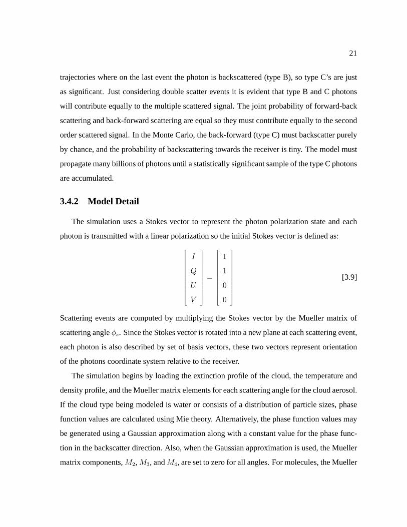
3.3 FOV Ratios, Gaussian Model-Monte Carlo Comparison . . . . . . . . . . . . . 28

4.1 A diagram of the HSRL receiver . . . . . . . . . . . . . . . . . . . . . . . . . . 31

4.2 A ray diagram of the primary field stop and how it separates the narrow field ofview from wider fields of view. . . . . . . . . . . . . . . . . . . . . . . . . . . . 32

5.1 02/22/2001, Altitude vs. time image of aerosol backscatter cross-section, from01:14 to 04:53 UT. . . . . . . . . . . . . . . . . . . . . . . . . . . . . . . . . . 38

5.2 02/22/2001, Altitude vs. time image of aerosol depolarization, from 01:14 to04:53 UT. . . . . . . . . . . . . . . . . . . . . . . . . . . . . . . . . . . . . . . 39

5.3 02/22/2001, 02:17:36-02:41:22 UT, mean cirrus backscatter cross section and sta-tistical errors. . . . . . . . . . . . . . . . . . . . . . . . . . . . . . . . . . . . . 40

5.4 02/22/2001, 02:17:36-02:41:22 UT, simple optical depth and fractional errors. . . 41

5.5 02/22/2001, 02:17:36-02:41:22 UT, Multiple Scatter model results for all particlesizes. . . . . . . . . . . . . . . . . . . . . . . . . . . . . . . . . . . . . . . . . 44

5.6 02/22/2001, 02:17:36-02:41:22 UT,G(r), for all FOV, model and HSRL results. 45

vi

AppendixFigure Page

5.7 02/22/2001, 02:17:36-02:41:22 UTC, AWFOV ratios results for2200µrad, in-cluding statistical errors. . . . . . . . . . . . . . . . . . . . . . . . . . . . . . . 46

5.8 02/22/2001, 02:17:36-02:41:22 UT, AWFOV ratios results for503µrad and963µradFOVs, including statistical and FOV errors . . . . . . . . . . . . . . . . . . . . 47

5.9 02/22/2001, 02:17:36-02:41:22 UT, AWFOV ratios results for296µrad, includ-ing statistical errors. . . . . . . . . . . . . . . . . . . . . . . . . . . . . . . . . 49

AppendixFigure

A.1 A diagram of the HSRL transmitter . . . . . . . . . . . . . . . . . . . . . . . . 56

B.1 Conceptual diagram of the HSRL wide field receiver . . . . . . . . . . . . . . . 60

vii

ABSTRACT

High Spectral Resolution Lidar (HSRL) measurements of cirrus cloud extinction and mul-

tiple scattering are used to determine cloud effective particle size. Multiple scattering is sig-

nificant in clouds because as the transmitted laser pulse travels through the cloud, half of the

single scattered energy from the cloud particles is contained within the forward diffraction

peak. This scattered energy propagates along with the transmitted beam and contributes to

the lidar signal. The width of the diffraction peak can be determined from HSRL multiple

scattering measurements, and since the diffraction peak width is proportional to the particle

cross-sectional area, particle size information can be obtained. The multiple scattering contri-

bution to the lidar signal depends on the transmitter divergence, receiver field-of-view, cloud

extinction profile, effective particle size, and the scattering phase function in the backward

direction. The HSRL transmitter divergence and receiver field-of-view are determined ex-

perimentally from system calibrations, and the extinction profile is provided from HSRL mea-

surements. The effective particle size and backscatter phase function information are unknown

parameters and in order to determine the effective particle size, backscatter phase function in-

formation must be provided. If the backscatter particles are molecules then the backscatter

phase function information can be provided from Rayleigh scattering theory. Using the HSRL

it is possible to only measure photons that have backscattered from molecules.

An approximate analytic model is used to calculate the multiple scatter contribution using

the HSRL-measured extinction profile for several effective particle sizes. The model results

viii

are then compared to the HSRL multiple scattering results to find the set of model results that

best fit the HSRL data for a specific effective particle size.

Presented are the first measurements of HSRL molecular multiple scattering from Febru-

ary 22, 2001 in Madison, Wisconsin. Comparisons with an approximate analytical multiple

scatter model indicate that the cirrus cloud observed during the period 02:17-02:41 UT had an

effective radius of 70± 10µm, which is a reasonable value for a cirrus cloud particle size.

1

Chapter 1

Introduction

1.1 Motivation

Cirrus clouds are important modulators of radiation in the earth-atmosphere system be-

cause they scatter incoming solar radiation and absorb outgoing longwave radiation. Even

though most cirrus clouds are optically thin, their location high in the troposphere, above most

other clouds, and large global coverage (> 30%, (Wylie et al., 1994)) means that their global

radiative impact can be quite significant. Depending on the cloud altitude, effective particle

size, and optical depth, the net radiative forcing can cool or warm the planet (Stephens and

Webster, 1981). Using International Satellite Cloud Climatology Project (ISCCP) C1 cloud

data and Earth Radiation Budget Experiment (ERBE) broadband energy flux data Hartmann

et al. (1992) produced global estimates of cloud radiative forcing by cloud type. This analysis

shows that the sign and magnitude of radiative cloud forcing varies with cloud optical depth,

altitude, time of year and geographical location. However, these analyses do not provide in-

formation on how cirrus clouds respond radiatively to changes in the Earth’s climate. Whether

cirrus clouds warm the earth in response to global warming (positive feedback), or cool the

planet (negative feedback), remains to be determined (Stephens et al., 1990; Wielicki et al.,

1995; Lindzen et al., 2000).

Cirrus cloud radiative properties depend on the cloud microphysical properties, such as

particle size, particle shape, and vertically integrated ice-water-content, the ice-water-path

(IWP). The relationship between the microphysical and optical properties is still poorly de-

scribed, because there is relatively little data of cirrus cloud microphysics properties. Little of

2

this data exists because measurements of cirrus cloud microphysical properties are difficult to

make since the clouds are found at high altitudes and are often tenuous. More measurements

of cirrus cloud microphysical and optical properties are required for a better understanding of

the role of cirrus in the radiation balance of the earth-atmosphere system and to model climate

change (Stephens et al., 1990).

The purpose of this thesis is to demonstrate a new method of measuring cirrus cloud ef-

fective particle size from lidar multiple scattering1 and extinction measurements, using the

University of Wisconsin High Spectral Resolution Lidar (HSRL). The effective radius is de-

termined by measuring the width of the diffraction peak from HSRL multiple field-of-view

molecular backscatter measurements. The molecular backscattering events depend only on the

diffraction peak width and the extinction profile and do not depend on the shape or magnitude

of the backscatter phase function of the cirrus particles. The multiple scattering contribution

is significant in clouds because as the transmitted laser pulse travels through the cloud, half

of the single scattered energy from cloud particles is contained within the forward diffraction

peak. This scattered energy propagates along with the transmitted beam and contributes to

the lidar signal (see figure 1.1). The diffraction peak width is inversely proportional to the

number weighted average cross-sectional area (van de Hulst, 1957), which is directly related

to the effective particle size.

The effective particle size is a representation of the cloud particle size distribution. In the

most general form, the effective particle size or effective radius,ae, is the number weighted

average volume divided by the number weighted average cross-sectional area for an ensem-

ble of cloud particles. For ensembles of irregularly shaped particles such as ice crystals, the

exact mathematical relationship between the size distribution and the effectiveradiusis some-

what obscure, since a radius is not well defined, see Wyser (1998). If the cloud particles are1Multiple scattering is a term to define the physical process of a photon that scatters from more than one

aerosol or molecule before returning to the lidar receiver.

3

spherical the effective radius can be defined as:

ae =

∞∫0

a3n(a)da

∞∫0

a2n(a)da=〈a3〉〈a2〉 [1.1]

Wheren(a) is the size distribution of the cloud particles; the number of particles as a function

of radius,a.

1.2 Background: Lidar Instruments and the HSRL

Light Detection and Ranging (lidar) instruments have long been used to make measure-

ments of cloud altitude, cloud depth, aerosol2 extinction (optical depth), and aerosol backscat-

ter cross-section. A lidar works by sending a short pulse of light into the atmosphere, and

as this pulse propagates along, some of the light is scattered back towards the receiver. For

visible wavelengths of light, scattering occurs for both aerosols and molecules. The intensity

of the received light is measured versus time, and since the velocity of light is known this

provides a profile of the received power versus range.

A fundamental problem of traditional lidar systems is that to obtain profiles of aerosol

extinction,a priori information about the relationship between backscatter and extinction must

be used, where,

βe = the extinction cross-section, per unit volume,m−1;

β′ = βePa(π)

4πthe backscatter cross-section, per unit volume,m−1sr−1;

Pa(π) is the backscatter phase function. The most notable lidar inversion technique relies on

a power law relationship between backscatter and extinction (Klett, 1981). The power law is

based on mathematical convenience rather than physical relationships. For example, in a given

scattering volume ifβe is fixed, the size distribution, particle shapes, and index of refraction

can be changed to produce almost any value ofβ′. Thus, profiles of extinction generated using2In this paper aerosols include both cloud droplets/crystals and macroscopic airborne particles (dust, pollen,

soot, etc.)

4

θs

I( )θ θs

Energy DistributionTransmitted Beam

ScatteringMedium

θ

ρ

Lidar

θ

C

B

A

Figure 1.1 Lidar scattering geometry. The grey shaded area represents the angular distributionof transmitted energy of the laser transmitter,θs is thee−1 point of the distribution, I is theradiance,W ·m−2sr−1. The anglesθ andρ represent the narrow, and wide field-of-view of thereceiver. The photon pathA shows a single scatter event.B andC show examples of possiblephoton trajectories that scatter from more than one particle (multiple scattering).B shows atrajectory where the photon backscattered on thelastevent before returning to the receiver.Cshows a photon path where the photon backscattersbeforehigher order scattering events.

5

the Klett method may have large errors (Mitev et al., 1992). The HSRL was developed to

overcome this fundamental limitation by separating the received signals into their molecular

and aerosol scattering components, (Shipley et al., 1983; Grund, 1987; Piironen, 1994). Using

Rayleigh scattering theory and an atmospheric temperature and density profile, the measured

molecular signal provides a known target at each altitude from which the aerosol backscatter

cross-section can be determined. The aerosol extinction profile can also be determined by

comparing the measured molecular signal to the molecular signal calculated in the absence of

aerosol extinction. Error bars can be calculated for each data product without relying on as-

sumed relationships between extinction and backscatter, because these measurements depend

only on statistical (photon counting) errors, system alignment errors, and calibration errors.

Also, lidar systems that can measure molecular Raman scattering can provide calibrated

profiles of aerosol extinction and backscatter.

1.3 Lidar Multiple Scattering

When making atmospheric measurements with a lidar system, the multiple scattering con-

tribution is usually treated as an error term when deriving the extinction profile. The capability

of the HSRL to measure the multiple scatter contribution for several receiver fields-of-view

allows this “error” term to be utilized as a powerful source of information about the cloud mi-

crophyics. Eloranta (1967) conducted some of the earliest multiple scattering lidar research,

and provided both the mathematical framework for modeling the double scattered lidar return

and made model comparisons with lidar measurements of fogs and hazes. Eloranta (1967)

also showed that the size distribution,n(a), of fogs and hazes could be determined using this

method. Also, at that time it was still not generally accepted nor understood that multiple scat-

tering contributed significantly to the single scattered lidar return thus affecting measurements

of extinction and backscatter. Work by Liou and Schotland (1971) seemed to indicate that

the multiple scattering contribution would in fact be small compared to the single scattered

lidar return, even for large receiver fields-of-view (FOV). This result was contradicted and

6

found to be incorrect by the work of Eloranta (1972), who presented an exact analytical solu-

tion for double scattered photons and showed that the multiple scatter contribution would be

roughly ten times greater than that presented by Liou and Schotland (1971). Eloranta (1972)

had also suggested that it may be possible to determine the width of the forward diffraction

peak with lidar measurements. Since then several investigators have developed models that

can describe the multiple scattering contribution as a function of receiver FOV, transmitter

divergence, cloud optical depth, effective particle size and scattering phase function in the

backscatter direction. (Eloranta, 1998; Bissonnette, 1996).

Several investigators have also demonstrated the use of lidar multiple scattering measure-

ments to determine the effective radius,ae, and the particle size distribution,n(a), of clouds.

Allen and Platt (1977) presented a description and measurements from single channel lidar

system. They showed that multiple scattering from water and cirrus clouds could be mea-

sured, and that it varied with receiver FOV. Later, Bissonnette and Hutt (1995); Roy et al.

(1997) demonstrated that lidar multiple scattering measurements could provideae, andn(a)

for water clouds, and made comparisons with aircraftin situ measurements. These measure-

ments, while successful, have been limited to clouds at low altitudes (< 2km), because of

instrument limitations. Benayahu et al. (1995) also reported a technique to measure the cloud

droplet size distribution,n(a), in water clouds. This technique required near horizontal point-

ing direction for the lidar so as to probe the cloud from the side, son(a) would not vary with

range (i.e. altitude). They only considered second order scattering, and were limited to small

optical depths. Yet another technique is described by Roy et al. (1999) to measuren(a), at

cloud base from lidar measurements of depolarization as a function of the receiver FOV. This

method however assumes the cloud is optically thin (optical depth< 1), since only second

order scattering is considered, and that the scattering particles are spherical.

The particle size measurement techniques presented above require information about the

backscatter phase function,P(π), of the backscattering particles in order to determinen(a),

or ae. This is a necessary requirement, since the photons that are most likely to contribute

to the lidar signal undergo only one large angle scattering event, (i.e. the scattering angle,

7

θs, ≈ π). For single scattering the photons that contribute scatter precisely at an angle ofπ,

so the single scattered return depends onP(π). The multiple scattered lidar signal must also

depend onP(θs ≈ π), and for most multiple order scatter events the backscattering angle

will be less thanπ in order to return the photon to the receiver. The result is that the multiple

scattered signal depends on bothP(π), and〈P(π)〉n. Where〈P(π)〉 is the average backscatter

phase function of the backscattering particles, encountered by the multiple scattered photons

of scattering order,n. Since the multiple scatter contribution depends on both the width of the

forward diffraction peak and〈P(π)〉, 〈P(π)〉 must be assumed or measured so the width of

the forward diffraction peak can be determined. If the backscattering particles are spherical

aerosols and a size distribution is specified, Mie theory can provide backscatter phase function

information. For irregularly shaped aerosols such as ice crystals, the particle shapes and size

distribution information is necessary to provide the backscatter phase function. Even with this

information, the phase function could only be modeled3, or perhaps estimated from laboratory

measurements. However, if the backscattering particles are molecules, the scattering phase

function is known to be nearly isotropic. BothP(π) and〈P(π)〉 are provided by Rayleigh

scattering theory.

1.4 The Technique

The technique presented in this thesis utilizes the ability of the HSRL to simultaneously

measure multiple scattered photons backscattered from atmospheric molecules and cloud ex-

tinction. An approximate multiple scatter model (see section 3.3) is used to calculate the

multiply scattered lidar return as a function of the receiver FOV and particle size, given the

parameters of the cloud extinction profile, receiver FOV, and transmitter divergence. Then,ae

is used as a variable to optimize the fit between HSRL observations and the model data. When

the model results are in agreement with the observations, the value ofae used for the model

calculations is assumed to representae of the cloud.3This is an enormous field of study, the details of which are beyond the scope of this thesis. Much information

about this topic can be found in Mishchenko et al. (2000)

8

1.5 Overview

This section provides a brief overview of the remaining chapters of this thesis. In chapter

2, lidar theory and HSRL principles will be discussed. Chapter 3 will describe three different

multiple scattering models, the last of which is a Monte Carlo scheme. The last section shows

a numerical comparison of the models. Chapter 4 will describe the method for HSRL multiple

scattering measurements and how to present the data so that it can be easily compared with the

multiple scattering model results. Chapter 5 shows the first HSRL measurements of molecular

multiple scattering from 22 February 2001 in Madison, Wisconsin, and the profiles of cloud

extinction necessary to run the multiple scatter model. Chapter 6 shows the model results

from 22 February 2001, and Chapter 7 presents a comparison of the model results and HSRL

measurements.

9

Chapter 2

Theory

2.1 Introduction

The purpose of this chapter is to provide the background information necessary to under-

stand how profiles of extinction cross-section , optical depth, backscatter cross-section, and

depolarization are derived from HSRL measurements. Starting with a general form of the

lidar equation, the molecular and aerosol components can be separated allowing these param-

eters to be derived. Two methods are included to derive the optical depth. The first, termed

the simple optical depth, depends only on the measured molecular signal, and is sensitive to

multiple scattering contributions to the lidar signal. The second method uses a vertically aver-

aged value of the backscatter phase function to derive the extinction profile, and if the cloud

is transparent to the lidar then the uncertainty in the derived extinction profile, from multiple

scatter contributions, will be significantly reduced.

2.2 Lidar Equation

This section defines the lidar equation, shown in terms of the number of received photons,

rather than power received. A derivation of this equation can be found in Measures (1988).

N(r, fov) = F (r, fov)No(fov)cA

2r2

(3

8πβm(r)+βa(r)

Pa(π, r)

4π

)e−2τ(r)+M(r, fov)+b(fov)

[2.1]

where,

N(r, fov) = number of photons incident on the receiver from range r, inside FOV,fov;

10

F (r, fov) = a geometrical factor, which depends on the receiver optics

and the transmitter beam divergence;

No(fov) = number of transmitted photons within the FOV,fov;

c = speed of light,ms−1;

A = area of receiver, m2;

βa(r), βm(r) = aerosol and molecular scattering cross sections

per unit volume from range r, respectively,m−1

3

8π= molecular backscatter phase function, sr−1;

Pa(π, r)

4π= aerosol backscatter phase function from range r, sr−1;

τ(r) = optical depth of the layer between rangesr1, andr2,

is given by∫ r2

r1

βe(r′)dr′,

βe(r) = total extinction cross section per unit volume at range r, m−1;

M(r, fov) = multiple scattering contribution (See section 3);

b(fov) = background signal;

The dependence of the termsN(r, fov), M(r, fov), b(fov) andF (r, fov) on FOV is explic-

itly indicated in this work, since the HSRL operates with several receiver FOVs, not just one

fixed receiver FOV. The termF (r, fov) accounts for the fact that at close ranges the telescope

is out of focus. This is a dimensionless quantity and is less than unity within 4 km of the

HSRL receiver.

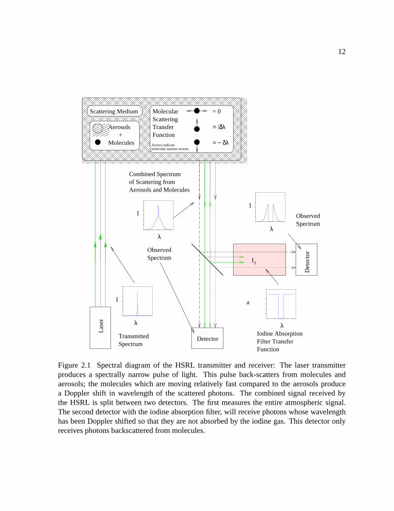
The HSRL is able to separate the molecular and aerosol signals by transmitting a spec-

trally narrow laser pulse, which is tuned to an absorption line of iodine gas. Thermal motion

of atmospheric molecules Doppler broaden the spectrum of the backscattered photons. The

aerosols which are much heavier and moving more slowly do not shift the backscattered spec-

trum significantly. Aerosol scattering is removed from one HSRL channel by removing the

center of the returned spectrum with an iodine gas absorption filter. (See figure 2.1).

11

2.3 HSRL Principles

The signals measured by the HSRL areSM andSA+M . SM is called the molecular channel,

since most of the photons measured by this channel have backscattered from molecules. There

is some leakage into this channel from photons that have backscattered from aerosols, because

not all the aerosol photons are absorbed by the iodine filter.SA+M is the combined channel,

measuring all molecular and aerosol photons. These signals can be inverted to provide the

individual aerosol and molecular signals as a function of range. The inversion requires system

coefficients derived from a spectral scan across the iodine absorption line while recording the

signals from both channels (Piironen, 1994). If the background light is subtracted from the

lidar signals and multiple scattering is ignored, the lidar equation above can be written:

For aerosols,

Na(r, fov) = F (r, fov)No(fov)cA

2r2βa(r)

Pa(π, r)

4πe−2τ(r) [2.2]

For molecules,

Nm(r, fov) = F (r, fov)No(fov)cA

2r2βm(r)

3

8πe−2τ(r) [2.3]

From these two equations the following parameters can be derived.

The scattering ratio:

SR(r) =Na(r)

Nm(r)[2.4]

SR(r) does not depend on FOV, since the terms that depend on FOV in both equations of

Na(r, fov) andNm(r, fov), cancel.

The aerosol backscatter cross-section:

β′a(r) = βa(r)Pa(π, r)

4π= SR(r)βm(r)

3

8π[2.5]

The simple optical depth:

τs(r) = −1

2log

(Nm(r, fov)

NT (r)

)[2.6]

12

−10 −5 0 5 100

0.2

0.4

0.6

0.8

1

1.2

−10 −5 0 5 100

0.2

0.4

0.6

0.8

1

1.2

−10 −5 0 5 100

0.2

0.4

0.6

0.8

1

1.2

−10 −5 0 5 100

0.2

0.4

0.6

0.8

1

1.2

a

Iodine AbsorptionFilter TransferFunction

ScatteringMolecular

TransferFunction

= + δλ

= − δλ

= 0Scattering Medium

Arrows indicatemolecular motion vectors

Las

er

Combined Spectrumof Scattering fromAerosols and Molecules

Molecules

Aerosols+

I

I

λ

λ

I

TransmittedSpectrum

Detector

Det

ecto

r

SpectrumObserved

λ

I

ObservedSpectrum

λ

2

Figure 2.1 Spectral diagram of the HSRL transmitter and receiver: The laser transmitterproduces a spectrally narrow pulse of light. This pulse back-scatters from molecules andaerosols; the molecules which are moving relatively fast compared to the aerosols producea Doppler shift in wavelength of the scattered photons. The combined signal received bythe HSRL is split between two detectors. The first measures the entire atmospheric signal.The second detector with the iodine absorption filter, will receive photons whose wavelengthhas been Doppler shifted so that they are not absorbed by the iodine gas. This detector onlyreceives photons backscattered from molecules.

13

NT (r) ∝ F (r, fov)No(fov)cA

2r2βm(r)

3

8π

where the termNT (r) is the derived molecular signal is the absence of aerosol extinction .

NT (r) is calculated using pressure and temperature profiles provided by radio sonde mea-

surements, and molecular scattering theory.NT (r) is then scaled to the molecular profile

Nm(r, fov) at a range,ro, which is above the lidar overlap region (i.e.F (r, fov) = 1, above 4

km). τs is given the subscripts to designate it as the simple optical depth. Note that the simple

optical depth is the optical depth from the range,ro, not from the lidar.

The aerosol extinction profile may be calculated fromτs(r) by,

〈βa(r)〉 =τs(r2)− τs(r1)

r2 − r1

[2.7]

Where〈βa(r)〉 is the average value ofβa between range binsr1 andr2.

βa(r) may also be determined in another way and will minimize errors from multiple

scatter contributions as long as the total cloud optical depth does not exceed 3.0, the maximum

optical depth measurable with the HSRL. The following equation,

∫ r2

r1

β′a(r)

〈Pa(π)4π

〉dr = τs(r2)− τs(r1) [2.8]

will be satisfied when the correct value of the bulk backscatter phase function of the cloud

particles,〈Pa(π)〉/4π is used,r1 is the altitude of the cloud base, andr2 is an altitude several

kilometers above the cloud top where multiple scatter contributions to the signalNm(r, fov)

are small. Figure 2.2 shows a comparison of the integral in equation 2.8 using〈Pa(π)〉/4π =

0.027 and a profile ofτs(r) derived from HSRL measurements. Then the profile ofβa(r) is

calculated from,

βa(r) =β′a(r)

〈Pa(π)4π

〉 [2.9]

By calculatingβa(r) in this manner the error from multiple scattering contributions to the

the single scattered lidar signal can be minimized. The multiple scatter contribution to the

signalsNa(r, fov) andNm(r, fov) are proportional to the individual single scatter signals.

14

5 6 7 8 9 10 11 12 130

0.1

0.2

0.3

0.4

0.5

0.6

0.7

0.8

0.9

Opt

ical

Dep

th

5 6 7 8 9 10 11 12 1310

−8

10−7

10−6

10−5

Altitude (km)

Bac

ksca

tter

Cro

ss−

Sec

tion

(1/(

m *

sr)

)

Simple OD Integrated β

e

Figure 2.2 An example of the simple optical depth,τs(r), and the integrated extinction profile,τ(r), derived from HSRL measurements on 2/22/01. Also, plotted along with the profile ofβ′a(r). The effect of multiple scattering on the profile ofτs is seen as a systematic decrease inthe optical depth in and above the cloud.

Therefore the value ofSR(r) is relatively insensitive to multiple scattering effects. Used

alone, the multiple scatter contribution to the molecular signalNm(r) is significant enough

that in calculating the optical depth from equation 2.6 (i.e the simple optical depth) results in

a systematic decrease in the optical depth in and above the cloud, until 2-3km above the cloud

top where multiple scatter contributions are small. For example, figure 2.2 shows the simple

optical depthτs(r), is biased from multiple scattering contributions while the contribution to

the integrated extinction profile is small.

Finally, in the aforementioned definitions, the aerosol signalNa(r, fov) is defined as a

single parameter, the HSRL however, also measures the change in the polarization state of the

received photons. The receiver separately measures the number of parallel(‖) and perpen-

dicular (⊥) polarized photons with respect to the transmitted linear polarization. Given the

15

measurementsNa‖(r, fov) andNa⊥(r, fov) the quantityδ, the depolarization, is defined as:

δ =Na⊥(r, fov)

Na‖(r, fov)[2.10]

This quantity is useful for unambiguously classifying the phase of the cloud particles. Since

water droplets are spherical, photons that backscatter from water droplets have the same polar-

ization. Depolarization measurements of water clouds typically range from 0.01 to 0.05. Since

ice crystals are irregularly shaped the polarization state of the scattered photon is rotated with

respect to the incident polarization. Depolarization values from ice range from 0.25-0.5. These

depolarization values represent measurements from the UW HSRL which has been designed

to minimize the multiple scatter contribution in the channels responsible for depolarization

measurements. Therefore, these depolarization values are not directly comparable to mea-

surements with lidar systems that have different receiver FOVs. The depolarization ratio will

increase as multiple scattering increases, so measurements using larger receiver FOVs may

not be able to unambiguously classify cloud phase.

16

Chapter 3

Multiple Scattering

3.1 Introduction

The measured lidar signal consists of both single and multiple scattered photons. The

multiple scattering contribution is significant when there are clouds in or below the scattering

volume, relative to the lidar. This is because as the transmitted laser pulse travels through the

cloud layer, half of the energy scattered by the cloud particles is contained within the forward

diffraction peak. This energy propagates along with the transmitted beam and contributes to

the lidar signal. At this time an exact analytic solution that describes the amount of multiple

scattering does not exist. However, there are several approximate models that can accurately

describe lidar multiple scattering.

The rest of this chapter is dedicated to describing two models based on analytical approx-

imations for multiple scattering and one Monte Carlo model. The final section shows the

results of a numerical comparison between all three models.

3.2 Infinite FOV Model

The approximate analytical solution to lidar multiple scattering formulated by Eloranta

and Shipley (1982) is dubbed in one of its forms as the infinite FOV model. When the FOV is

assumed to be large compared to the diffraction peak width of the particles the multiple scatter

contribution can be determined very easily.

17

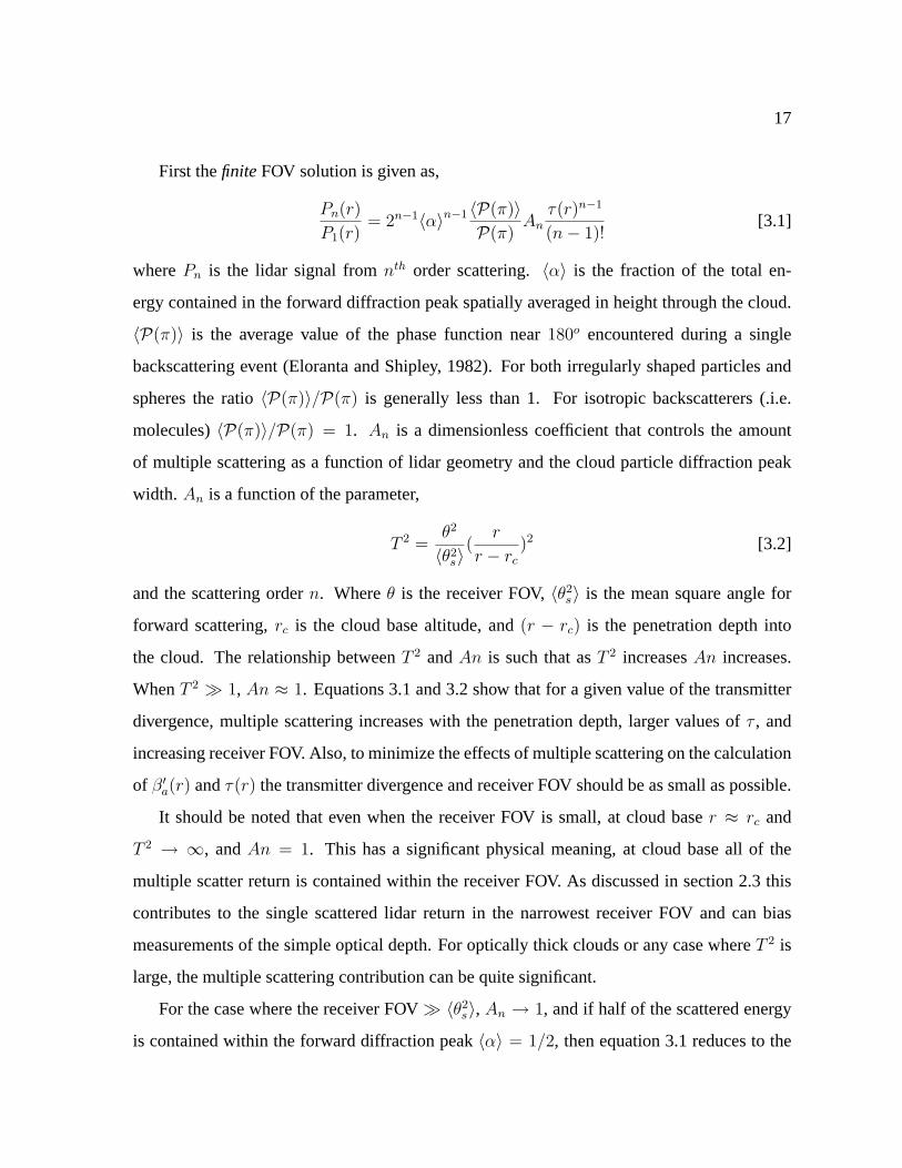
First thefiniteFOV solution is given as,

Pn(r)

P1(r)= 2n−1〈α〉n−1 〈P(π)〉

P(π)An

τ(r)n−1

(n− 1)![3.1]

wherePn is the lidar signal fromnth order scattering.〈α〉 is the fraction of the total en-

ergy contained in the forward diffraction peak spatially averaged in height through the cloud.

〈P(π)〉 is the average value of the phase function near180o encountered during a single

backscattering event (Eloranta and Shipley, 1982). For both irregularly shaped particles and

spheres the ratio〈P(π)〉/P(π) is generally less than 1. For isotropic backscatterers (.i.e.

molecules)〈P(π)〉/P(π) = 1. An is a dimensionless coefficient that controls the amount

of multiple scattering as a function of lidar geometry and the cloud particle diffraction peak

width. An is a function of the parameter,

T 2 =θ2

〈θ2s〉

(r

r − rc

)2 [3.2]

and the scattering ordern. Whereθ is the receiver FOV,〈θ2s〉 is the mean square angle for

forward scattering,rc is the cloud base altitude, and(r − rc) is the penetration depth into

the cloud. The relationship betweenT 2 andAn is such that asT 2 increasesAn increases.

WhenT 2 À 1, An ≈ 1. Equations 3.1 and 3.2 show that for a given value of the transmitter

divergence, multiple scattering increases with the penetration depth, larger values ofτ , and

increasing receiver FOV. Also, to minimize the effects of multiple scattering on the calculation

of β′a(r) andτ(r) the transmitter divergence and receiver FOV should be as small as possible.

It should be noted that even when the receiver FOV is small, at cloud baser ≈ rc and

T 2 → ∞, andAn = 1. This has a significant physical meaning, at cloud base all of the

multiple scatter return is contained within the receiver FOV. As discussed in section 2.3 this

contributes to the single scattered lidar return in the narrowest receiver FOV and can bias

measurements of the simple optical depth. For optically thick clouds or any case whereT 2 is

large, the multiple scattering contribution can be quite significant.

For the case where the receiver FOVÀ 〈θ2s〉, An → 1, and if half of the scattered energy

is contained within the forward diffraction peak〈α〉 = 1/2, then equation 3.1 reduces to the

18

infinite FOV equation:Pn(r)

P1(r)=〈P(π)〉P(π)

τ(r)n−1

(n− 1)![3.3]

Equation 3.3 depends on both the optical depth and the backscatter phase function ratio. If the

backscattering particles have an isotropic backscatter phase function, then this ratio is one and

the multiple scatter contribution depends only on the optical depth.

3.3 Gaussian Approximate Solution

The multiple scattering model describe here was developed by Eloranta (1998) and is

in fact a derivative of the infinite FOV model. This model is referred to as the Gaussian

model. Like the infinite FOV model the primary assumption is that each photon experiences

only one large angle scattering event. This means that photons are assumed to be scattered

within the forward diffraction peak and in the backscatter direction. No other photons are

considered. Given this assumption the ratio〈P(π)〉/P(π) is again used as a parameter. For

isotopic backscatters, like molecules, this ratio equals one. The second assumption is that a

Gaussian function represents the forward scattering diffraction peak. The form is:

P(θ)

4π=P(0)true

4πexp

(−θ2

θ2s

)[3.4]

WhereP(0)true/4π is the value of the phase function at zero degrees provided by Mie theory

or calculated as a function of the effective particle size. The value ofθs is determined explicitly

from the valueP(0) if we assume that equation 3.4 is integrated over the sphere and is equal

12, or rather that the diffraction peak contains half of the scattered energy. So,

∫

4π

P(θ)

4πdΩ = 1/2

yields,

〈θ2s〉 =

2

P(0)[3.5]

19

To generalize this for any arbitrary distribution of particle sizesn(a), the scattering cross

sectionβs can be defined as,

βs[λo, n(a)] = π

a2∫

a1

a2n(a)Qsc(λo, a)da [3.6]

whereQsc is the scattering efficiency factor. Then the average value of the phase function at

zero degrees may be calculated in following way after Deirmendjian (1969),

P(0) =4π

k2βs

a2∫

a1

n(a)I(0, a)da [3.7]

If we assume that the particles are large so thatQsc(λo) = 2 andI(0, a) = k4a4/8, where

k = 2π/λ, then equation 3.7 becomes:

P(0) =

πk2

2

a2∫a1

a4

8n(a)da

2πa2∫a1

a2n(a)da=〈a4〉〈a2〉

2π2

λ2

ae ≈ λ

π

√P(0)

2[3.8]

Where,ae = 〈a3〉〈a2〉 and the following assumption has been made:ae ≈

√〈a4〉〈a2〉 . This approxima-

tion is surprisingly robust and is not limited to the previous assumption that the particles are

spherical. Since in general the value of the scattered intensityI(0) in the forward direction

depends primarily on the cross-sectional particle area. For the remainder of this thesis the

effective particle size will be represented byae.

Assuming that the diffraction peak contains half of the forward scattered energy, has a

Gaussian shape, andP(0) = 2/〈θs〉, it is possible to derive an equation describing the ra-

tio of returned power of scattering ordern, divided by the single scattered returned power,

Pn(r)/P1(r). This ratio must be evaluated numerically and can be calculated given the fol-

lowing input parameters,βe(r), ae, βm(r), the receiver FOV, andθt the laser transmitter diver-

gence (full-angle). The numerical model used for the multiple scatter calculations has been

fully implemented by Eloranta, and the results computed for this paper were calculated using

this software.

20

3.4 Monte Carlo

This section describes the Monte Carlo simulation of lidar multiple scattering. The name

Monte Carlo comes from the city bearing that name and generally defines a statistical method

of evaluating mathematical or physical systems. This Monte Carlo simulation was developed

to investigate multiple scattering for lidar systems that are difficult or impossible to solve by

other approximate analytical models. The main purpose of this Monte Carlo was to validate

the Gaussian model, and the Gaussian model software. Part one gives a general overview of

this Monte Carlo, and part two describes the model in more detail.

3.4.1 Overview

In this application of the Monte Carlo method one photon is propagated at a time into the

atmosphere. The probability of when the photon scatters depends on the prescribed extinc-

tion profile. The scattering angle of each event is determined by Mie or Rayleigh scattering

theory, depending whether the scattering particle is an aerosol or molecule. Instead of prop-

agating each photon indefinitely until it returns to the receiver, at each scattering event the

photon is assumed to have returned to the receiver and is weighted according to the probabil-

ity of that event occurring. The photon is then scattered randomly and propagated to the next

scatter event, where it is again assumed to have returned to the receiver. At each scattering

event the photon properties are accumulated according to the FOV, range, scattering order,

and polarization. This methodology was chosen to minimize the number of accumulated pho-

tons necessary for a statistically significant multiple scattered signal, compared to a traditional

random walk scheme.

Even though this model calculates the partial return at each scattering event, photons that

have backscattered before a higher order scattering event and remain within the receiver FOV,

are rare (type C, see figure 1.1). The example in figure 1.1 shows just one type C trajectory,

a forward-back-forward trajectory would also be considered type C for third order scattering.

In the real atmosphere these types of photon trajectories are just as likely to occur as those

21

trajectories where on the last event the photon is backscattered (type B), so type C’s are just

as significant. Just considering double scatter events it is evident that type B and C photons

will contribute equally to the multiple scattered signal. The joint probability of forward-back

scattering and back-forward scattering are equal so they must contribute equally to the second

order scattered signal. In the Monte Carlo, the back-forward (type C) must backscatter purely

by chance, and the probability of backscattering towards the receiver is tiny. The model must

propagate many billions of photons until a statistically significant sample of the type C photons

are accumulated.

3.4.2 Model Detail

The simulation uses a Stokes vector to represent the photon polarization state and each

photon is transmitted with a linear polarization so the initial Stokes vector is defined as:

I

Q

U

V

=

1

1

0

0

[3.9]

Scattering events are computed by multiplying the Stokes vector by the Mueller matrix of

scattering angleφs. Since the Stokes vector is rotated into a new plane at each scattering event,

each photon is also described by set of basis vectors, these two vectors represent orientation

of the photons coordinate system relative to the receiver.

The simulation begins by loading the extinction profile of the cloud, the temperature and

density profile, and the Mueller matrix elements for each scattering angle for the cloud aerosol.

If the cloud type being modeled is water or consists of a distribution of particle sizes, phase

function values are calculated using Mie theory. Alternatively, the phase function values may

be generated using a Gaussian approximation along with a constant value for the phase func-

tion in the backscatter direction. Also, when the Gaussian approximation is used, the Mueller

matrix components,M2, M3, andM4, are set to zero for all angles. For molecules, the Mueller

22

matrix is calculated using:

M1(φ) =1

2(1 + cos(φ)2);

M2(φ) =1

2(cos(φ)2 − 1)

M3(φ) = cos(φ)

M4(φ) = 0.0 [3.10]

The probability distributions for choosing the scattering angle and the scattering distance are

also created. These are lookup tables generated so that only random numbers are necessary

at each scattering event to determine the scattering angle and distance traveled. The main

program loop has the following structure.

1. Pick initial direction based on transmitted Gaussian energy distribution.

2. Move photon to cloud base.

3. Pick random number to determine distance to scattering event. (From probability distri-

bution generated from extinction profile).

4. Move photon to scattering particle.

5. Determine if photon is within the receiver FOV.

6. Determine if particle is an aerosol or molecule. (From scattering cross-sections.)

7. Now assume photon scatters back to receiver.

(a) Calculate scattering angleφs back to receiver.

(b) Rotate photon Stokes vector into scattering plane, angleψ. (For scattering orders

> 2. The plane is defined by last and current scattering particle and the receiver.)

(c) Multiply photon Stokes vector by Mueller matrixM(φs).

23

(d) Calculate probability of photon traveling along this path back to receiver without

being extinguished. This becomes the photon weight.

w =cos(Φ)

r′2e−τ(z) [3.11]

WhereΦ is the angular location of the photon with respect to the z-axis.r′ is the

distance from the receiver to the photon, andτ(z) is the optical depth from the

altitudez to the receiver.

(e) Move photon to receiver.

(f) Rotate photon Stokes vector into original coordinate system of receiver.

(g) Record photon properties binned according to total distance traveled, scattering

order, and FOV:

P (l, n, fov) ∝ w · I [3.12]

P⊥(l, n, fov) ∝ w · (I −Q)

2

P‖(l, n, fov) ∝ w · (I + Q)

2

l andn are the path length and scattering order, respectively. The last two expres-

sions account for the linear polarization state of the received photon in terms of the

⊥ and‖ components with respect to the transmitted polarization.

Let photon continue along its original path.

8. Determine scattering angle,φs, from phase function probability distribution and load

appropriate Mueller matrix,M(φs).

9. Rotate photon Stokes vector into scattering plane, angleψ. (Picked from uniform prob-

ability distribution.)

24

10. Multiply Stokes vector by Mueller matrix,M(φs).

11. Normalize Stokes vector by component I.

12. Return to step 3.

The rotation and multiplication steps are performed using the following matrix multiplication

(steps 7b,7c and 9, 10)

I

Q

U

V

=

M0 M1 0 0

M1 M0 0 0

0 0 M2 M3

0 0 −M3 M2

0 0 0 0

0 cos(2ψ) −sin(2ψ) 0

0 sin(2ψ) cos(2ψ) 0

0 0 0 0

I0

Q0

U0

V0

[3.13]

Step 11, the Stokes vector normalization, is done to preserve the continuity that only one

photon is propagated at a time and the photon polarization state.

25

3.5 Model Comparison

This section shows a comparison of the Monte Carlo and multiple scattering models. This

was necessary because both the Monte Carlo and the Multiple Scatter model code had not

been rigorously tested for coding errors. A hypothetical cloud was created to perform this

comparison. The cloud optical and simulated lidar parameters used were:

Table 3.1 Cloud Optical Properties

Base 600 m

Top 900 m

ae(r) uniform, 25µ m

βa(r) uniform,3.33x10−3(m−1)

Total τ 1.0

Table 3.2 Transmitter, Receiver Specifications

Transmitter Div. (Gaussian)110µ rad

Receiver FOVs (wide 1) 10.3 mrad

(wide 2) 963µ rad

(wide 3) 296µ rad

(narrow) 110µ rad

The cloud properties were chosen to minimize the time required to accumulate a statis-

tically significant signal from multiple scattered photons in the Monte Carlo model. It was

necessary to accumulate4.8 · 1010 photons to generate good statistics.

The Monte Carlo model run consisted of 8 separate model runs of6.0 · 109 photons each.

The total computer time required was approximately 65 hours, see appendix A for computer

details. Figure 3.2 shows a comparison of the Monte Carlo, Gaussian, and infinite FOV mod-

els. The Monte Carlo results show the mean value ofPn/P1 for 2nd, 3rd, and 4th order scat-

tering. The error bars estimate±σ, the standard deviation in the mean, for all the model runs.

26

10−6

10−4

10−2

Ext

inct

ion

Cro

ss S

ectio

n (m

−1 ) β

eβ

M

600 700 800 900 1000 1100 12000

0.2

0.4

0.6

0.8

1

Opt

ical

Dep

th

Altitude (m)

Figure 3.1 Model Cloud Optical Properties

At this time the Monte Carlo does not provide a measurement of the statistical fluctuations in

the values ofPn.

The Monte Carlo, Gaussian, and infinite FOV model are in agreement (see figure 3.2). The

infinite FOV deviates slightly from the Monte Carlo and the Gaussian models, because these

models only approximate an infinite FOV with a value of 10.3 mrad. This is especially clear

for 3rd and 4th order scattering, above 900 meters altitude. Figure 3.3 shows the ratios for

three different fields of view. The plotted ratio is:

G(r) =P2(r, fovw) + P3(r, fovw) + P4(r, fovw)

P1(r, fovn) + P2(r, fovn) + P3(r, fovn) + P4(r, FOVn)[3.14]

27

0

0.5

1

1.5

P2/

P1

Monte CarloMS Model INF FOV

0

0.2

0.4

0.6

0.8

1

P3/

P1

600 700 800 900 1000 1100 12000

0.1

0.2

0.3

Altitude (m)

P4/

P1

Figure 3.2Pn/P1, Gaussian Model - Monte Carlo Comparison (10.3mrad FOV)

Wherefovw is the particular wide FOV,fovn is the narrowest receiver FOV. The multiple

scatter contribution tofovn is small, so that this equation can be approximated by,

G(r) ≈ P2(r, fovw) + P3(r, fovw) + P4(r, fovw)

P1(r, fovn)[3.15]

This comparison does not include the results from the infinite FOV model since the receiver

FOV can longer be considered infinite. The 0.963 mrad , and 0.296 mrad results show a large

decay in the multiple scattering contribution above the cloud top, this is due to the multiple

scattered photons leaving these FOV. Even with the large number of photons collected, in this

Monte Carlo run the 0.296 mrad FOV shows fairly poor statistics. However, a rough agreement

28

0

1

2

3(1

0.3

mra

d)

Monte CarloMS Model

0

0.2

0.4

0.6

0.8

1

(0.9

63 m

rad)

600 700 800 900 1000 1100 12000

0.05

0.1

0.15

0.2

(0.2

96 m

rad)

Altitude (m)

Figure 3.3 FOV Ratios,(P4 + P3 + P2)/P1 , Gaussian Model-Monte Carlo Comparison

between the two models can be seen. Also, the Gaussian model results are not smooth in this

case because of roundoff error in the calculation of the multiple scatter contribution. So,

these comparisons show that the Gaussian model can be used to determine the contribution of

multiple scattering to the lidar signal.

29

Chapter 4

Measurement and Data Analysis Techniques

4.1 Introduction

Values of the effective radius,ae, are inferred from the comparison of HSRL multiple

scattering data and Gaussian model results, computed using different values ofae. The HSRL

provides profiles of the aerosol backscatter cross-sectionβ′a(r), and extinction cross-section

βe(r), as shown in section 2.3. Given these profiles the Gaussian model can be used to compute

the multiple scatter contribution for different FOV and values ofae. The HSRL also provides

measurements ofM(r, fov), section 2 of this chapter discusses how this is accomplished.

Section 3 then describes how the ratiosG(r) are computed from measurements ofM(r, fov)

so they can be compared with the Gaussian model results ofG(r). The final section discusses

how the HSRL profile ofG(r) must be corrected for the relative efficiency factor between the

two detectors used to make single and multiple scattering measurements.

4.2 Measuring Multiple Scattered Photons: HSRL Receiver

This section describes features of the HSRL receiver required for multiple scattering mea-

surements. Further details about the HSRL can be found in appendix A, and in (Piironen,

1994). Figure 4.1 shows a schematic of the HSRL receiver setup. The receiver is split into

two major parts, the narrow field of view (NFOV) channels, and the annular wide field-of-view

(AWFOV) channels. The NFOV channels measure the single scatter lidar return, which are

used to derive the quantities ofβ′a(r), τ(r) andδ. This FOV is designed to be as small as pos-

sible to minimize the contribution from multiple scattered photons. The NFOV minimum size

30

is limited by the laser transmitter divergence, since the FOV must be large enough to collect a

large percentage of the single scattered return. Currently, the laser transmits with a Gaussian

beam profile with a divergence of 110µrad, full-anglee−1 width. The NFOV size is currently

set to 110µrad.

The FOV of the HSRL is controlled by an aperture placed at the focal plane of the tele-

scope. This is because an incoming photon with angleθ with respect to the optical axis of the

telescope will be mapped to a position,y, on the focal plane. The relationship is expressed

mathematically as,y ∼ f · θ, where f is the effective focal length of the telescope (figure B.1).

The limiting aperture for the NFOV is shown in figure 4.1 and in an expanded view in figure

4.2, the location of the aperture is in fact at an image of the telescope prime focus. The NFOV

aperture is an 800µm hole in center of a flat mirror. Photons that fall outside the NFOV are

redirected by the mirror to the AWFOV channels. This allows both normal HSRL and multiple

scattering measurements to be made simultaneously with a minimum amount of signal loss

(i.e. as opposed to splitting the entire signal off before the NFOV aperture.)

The AWFOV aperture is placed at an image of the telescope prime focus before the NFOV

aperture. This aperture can be changed in diameter and is controlled by the data acquisition

system. Typically the aperture diameter is changed after every averaging period. One averag-

ing period orshot is the sum of 4000 individualseededlaser pulses.Seededlaser pulses are

those that have the proper spectral characteristics necessary to separate the HSRL signal for

aerosol and molecular scattering. During operation the laser is typically seeded 70% of the

time, fired at a rate of4kHz. Each lasershottakes approximately 3 seconds to acquire. The

AWFOV aperture is stepped every shot through a cycle of 3 to 4 different diameters/FOVs (i.e.

0.3, 0.5, 1.0, 2.0, 0.3, 0.5...mrad). This is done to simplify data analysis and to minimize the

time between observations with each AWFOV.

31

AW

FO

V

NF

OV

To

Atm

osph

ere

Ref

ocus

ing

Len

s

Opt

iona

l

Fabr

y−Pe

rot

Eta

lon

Inte

rfer

ence

Fi

lter

Mir

ror

Mot

oriz

ed

Hol

ogra

phic

D

iffu

ser

Hol

ogra

phic

D

iffu

ser

D 1

Pola

rizi

ngB

eam

Spl

itter

s

Dec

tect

or D

escr

iptio

ns

D 4

= A

WFO

V C

ombi

ned

Cha

nnel

, Ham

amat

su R

5600

U P

MT

D 2

= C

ombi

ned

Cha

nnel

, Ham

amat

su R

7400

P PM

T

D 1

= I

odin

e R

ejec

tion

(Mol

ecul

ar)

Cha

nnel

,

D 3

= I

odin

e R

ejec

tion

(AW

FOV

Mol

ecul

ar)

Cha

nnel

,

EG

+ G

SPC

M, A

vala

nch

Phot

odio

de

Tho

rn E

MI

9853

B/3

50 P

MT

NFO

V A

pert

ure

(Mir

rore

d)

Iodi

ne C

ell

D 2

D 4

Gla

re S

top

Ape

rtur

e fo

r A

WFO

VC

ompu

ter

Con

tolle

d

Bea

m S

plitt

ers

0.5m

Pri

mar

y

λ/4

Iodi

ne C

ell

From

Las

er T

rans

mitt

er

D 3

Figure 4.1 A diagram of the HSRL receiver

32

Computer ControlledAperture for AWFOV

Collimating LensTurning Mirror

Primary Field StopCollimating Lens Focusing Lens

Figure 4.2 A ray diagram of the primary field stop and how it separates the narrow field ofview from wider fields of view. The rays represent possible paths of photons that scatteredback to the receiver from outside(green) or inside(blue) the NFOV. NFOV.

33

4.3 Deriving the AWFOV Ratio Equation

This section describes how the ratiosG(r) are computed from measurements ofM(r, fov)

so they can be compared with the Gaussian model results ofG(r). The following two equa-

tions describe the lidar signals measured with the AWFOV molecular channel, and the narrow

molecular FOV channels, respectively.

NΨ(r) =((eρ − eθ) + MΨ(r)

)R(r)CΨ [4.1]

Nθ(r) =(eθ + Mθ(r)

)R(r)Cθ [4.2]

where

NΨ(r) = the number of photons received in the wide annular FOV as a function of range.

This is a measured quantity.

Nθ(r) = the number of photons received in the narrow FOV channel as a function of range.

This is a measured quantity.

Ψ = ρ− θ,the full-angle receiver AWFOV.

eθ = (1− exp(−θ2/θt)2) the percentage of energy transmitted within the FOVθ.

θt is the transmitter divergence full-anglee−1 width.

eρ = the percentage of energy transmitted within the FOVρ.

R(r) = NocA

2r2

(3

8πβm(r)

)e−2τ(r) [4.3]

The total Rayleigh component of the signal, including aerosol

extinction and range dependence.

No = the number of transmitted photons.

MΨ(r) = the signal from aerosol multiple scattering in the wide annular FOVΨ.

Defined as a percentage of the total Rayleigh signal.

Mθ(r) = the signal from aerosol multiple scattering in the narrow FOVθ.

34

Defined as a percentage of the total Rayleigh signal.

CΨ = annular-wide FOV detector efficiency and optical transmission factor.

Cθ = narrow FOV detector efficiency and optical transmission factor.

If the we use the lidar signals from a region where there is little or no aerosol single or

multiple scattering a constantk can be defined as:

k =NΨ(rmol)

Nθ(rmol)=

(eρ − eθ)R(r)CΨ

eθR(r)Cθ

=(eρ − eθ)CΨ

eθCθ

[4.4]

The ratios G(r) are calculated using a form of the following equation. This form was

chosen to minimize the contribution from single scattering in the annular FOV.

G(r) =NΨ(r)− kNθ(r)

Nθ(r)[4.5]

By expanding this equation it can be seen that the single scattered component is removed from

the numerator.

G(r) =((eρ − eθ) + MΨ(r))R(r)CΨ − k(eθ + Mθ(r))R(r)Cθ

(eθ + Mθ(r))R(r)Cθ

=((eρ − eθ) + MΨ(r))CΨ − (eρ−eθ)CΨ(eθ+Mθ(r))Cθ

eθCθ

(eθ + Mθ(r))Cθ

=(MΨ(r)− (eρ − eθ)Mθ(r))CΨ

(eθ + Mθ(r))Cθ

[4.6]

The ratios must be corrected for the termCΨ/Cθ, the relative detector and optical trans-

mission factor. This can be computed by inverting the equation used to determinek and its

computed value.CΨ

Cθ

=keθ

(eρ − eθ)[4.7]

Note that the transmitter divergence,θt and the receiver FOV,θ andρ, must also be used to

calculate this ratio. Finally, the computed ratios are:

G′(r) =G(r)

CΨ

Cθ

=NΨ(r)− kNθ(r)

Nθ(r)

(Cθ

CΨ

)[4.8]

35

4.4 Correcting for the Relative Detector Efficiencies

The HSRL AWFOV ratios must be properly scaled by the relative detector efficiency and

optical transmission factor, which is expressed as a single quantity, the relative channel effi-

ciency. It is impractical to measure the channel efficiencies directly, so the relative efficiency

is measured instead.

4.4.1 Method I

The first method is to use the equation 4.7. The value ofk is calculated from equation 4.4,

k = NΨ(r)/Nθ(r), from lidar measurements in a region absent of aerosol scattering. The

transmitter beam divergence has been estimated from measurements to have a Gaussian profile

containing 88% of the total energy with a divergence of110±10µrad. Using this value for the

transmitter divergence and a NFOV width of 110µrad, the relative channel efficiency factor

C ′ is calculated to be0.34± 0.10.

4.4.2 Method II

The second method uses information only collected from the calibration source. The cal-

ibration source is an aperture designed to uniformly illuminate the AWFOV and NFOV aper-

tures1. The signal measured from the calibration source is proportional to the aperture area

and the channel efficiencies. This method assumes that the calibration source is uniformly

illuminated, and that all optical elements in the HSRL receiver have been correctly aligned.

C ′ =Sρ−θ

Sθ

Aθ

(Aρ − Aθ)[4.9]

WhereAθ is the area of the narrow FOV aperture imaged onto the AWFOV aperture, andAρ

is the area of the annular wide field of view aperture. The value ofC ′ measured with this

technique is0.31± 0.09.1See Piironen (1994) for further information about the calibration source

36

4.4.3 Method III

The final and preferred method to correct for the relative channel efficiency does not de-

pend on system calibrations. From the infinite FOV model, equation 3.3, no longer depends

on 〈θs〉 which is proportional toae. So for ranges in the cloud wherer À (r − rc), the ratio

(P4 + P3 + P2)/P1 is independent ofae. So the ratioG(r) computed from HSRL measure-

ments should have the same slope if the correct value ofC ′ is used. In this caseC ′ was varied

until G(r) has the same slope as(P4 + P3 + P2)/P1. As long as at least one receiver FOV is

large compared to〈θs〉, this relationship can be used. Figure 5.5, the 2200µrad FOV panel,

demonstrates this effect. These are the Gaussian model results computed from the extinction

measurements on February 22, 2001, as a function ofae. Once the multiple scattering equi-

librium is obtained a few hundred meters from cloud base, all the ratios have the same slope.

Since this FOV is not infinite, at farther ranges the multiple scatter signal decays as photons

exit the FOV.

The value ofC ′ found to give the best fit slope to the model results from 2/22/01, is 0.35.

This is within the limits of experimental error inC ′ computed using both methods I, and II

above.

37

Chapter 5

Results

5.1 February 22, 2001 Measurements

On February 22, 2001 the HSRL collected data from 01:14 UT until 04:53 UT, in Madi-

son, Wisconsin (43.07 N, 89.38W). During this period the AWFOV aperture was operated to

collect multiple scattering data. High altitude ice clouds (cirrus) were observed during this pe-

riod. Figure 5.1 shows altitude versus time image of aerosol backscatter cross-section(β′a(r))

derived from inverted HSRL data. Figure 5.2 shows and altitude versus time image from the

same period of inverted aerosol depolarization.

Since the multipley scattered signal measured with the HSRL is quite small, the data must

be averaged to ensure that the statistical errors (photon counting) are small. In this case 24

minutes, 400 laser shots, were required to reduce statistical errors to an acceptable level. Since

four AWFOVs were used the total number of shots summed for each channel was 100. The

averaging period was from 02:17:36 until 02:41:22 UT. During this period the cloud base

remained relatively constant and uniform. Also, the region below the cloud layer was free

from other cloud layers or aerosols.

Multiple scatter calculations require the atmospheric profile ofβa(r). Since the maximum

optical depth of this section of the cloud was 0.7, it was possible to calculateβa(r) from

equation 2.9. Figure 2.2 (shown previously) is a plot of the simple optical depth,τs(r), and

the integrated extinction,βa(r), calculated using〈Pa(π)/4π〉 = 0.027.

Although the errors inβa(r) were not determined explicitly, the errors inβ′a(r) and τs

were calculated to illustrate the largest possible sources of error inβa(r). Figure 5.3 shows

38

Figure 5.1 02/22/2001, Altitude vs. time image of aerosol backscatter cross-section showingcirrus clouds from 01:14 to 04:53 UT. The period used to estimate the effective particle size isfrom 02:17:36 to 02:41:22 UT. This area is delineated by vertical blue lines.

the derived profile ofβ′a(r) and the associated statistical errors. Figure 5.4 showsτs, as well

as the contribution of both statistical errors and errors from using a atmospheric temperature

profile that may not be representative of the atmospheric temperature profile over Madison,

WI, during the HSRL operation. During normal HSRL operations radio sonde profiles from

Green Bay, WI are used for temperature and density information. A difference between the

true vertical lapse rate through the cloud layer, and the lapse rate of the temperature profile

used to calculate the theoretical molecular profile,NT (r), is a significant source of error for

the simple optical depth,τs(r). A constant difference between the true temperature profile and

39

Figure 5.2 02/22/2001, Altitude vs. time image of aerosol depolarization, from 01:14 to 04:53UT. The values of depolarization, (≈ 0.4), indicate that the cloud consists of ice particles forthe entire period, 01:14 to 04:53 UT. The period used to estimate the effective particle size isfrom 02:17:36 to 02:41:22 UT. This area is delineated by vertical blue lines.

the one used to calculateNT (r) is nota significant source of error sinceNT (r) is scaled to the

measured molecular signal at reference altitude below the cloud.

The error in the lapse rate was estimated by computing the maximum difference in the

lapse rates between 6 and 10 km, from the three different soundings. The maximum difference

was determined to be1/km. When including both the statistical and lapse rate errors, the error

in the simple optical depth was less than 3% at 12 km. This is the reference altitude used to

determine the profile of integrated aerosol extinction.

40

10−8

10−7

10−6

10−5

5

6

7

8

9

10

11

12

13

14

15

Aerosol Backscatter Cross Section (1/(m*sr))

Alti

tude

(km

)

10−3

10−2

10−1

100

Fractional Error

Figure 5.3 02/22/2001, mean cirrus backscatter cross section and statistical errors for theperiod 02:17:36 to 02:41:22 UT.

41

0 0.2 0.4 0.6 0.8 15

6

7

8

9

10

11

12

13

14

15

Simple Optical Depth

Alti

tude

(km

)

10−2

10−1

100

Fractional Error

Total StatisticalLapse Rate

Figure 5.4 02/22/01, mean simple optical depth and fractional errors for the period 02:17:36 to02:41:2 UT. The errors shown are from photon counting (statistical) errors and from errors dueto using a atmospheric temperature profile that may not be representative of the temperatureprofile over Madison, WI, during the HSRL data collection.

42

5.2 Gaussian Model Results

The multiple scatter model was run with the parameters given in table 5.2. The 84 separate

data files (1 for each FOV and particle size) required 8 hours to complete running 2 processes

on the computer describe by Table A.

Table 5.1 Multiple Scatter Model Parameters for 02/22/2001, 02:17-02:41 UT.

Transmitter Div. 110µrad

Receiver FOV (narrow) 110µrad

(Annular wide 1) 296µrad

(Annular wide 2) 503µrad

(Annular wide 3) 963µrad

(Annular wide 4) 2200µrad

(Annular wide 5) 10.3mrad

ae(r) uniform in altitude, 40..5..110µm

βm(r) Green Bay, WI, 00:00 UT Sounding.

βa(r) Values computed from section 5.1.

Max scattering order 4

The results from this model run are summarized by figure 5.5. This figure shows the

AWFOV ratios,G(r), for each FOV as described in section 4.3 by equation 4.8. Its purpose is

to demonstrate the variability of the AWFOV ratios with both particle size and FOV. The first

thing to note is that for a given value of effective particle size the maximum value of the ratio

G(r) decreases with smaller FOVs. This is because with each scattering event the probability

that a photon will leave a given FOV increases. So, large FOVs contain more photons of

higher scattering order than small ones.

By just considering one FOV, the smaller particles always have the smallest peak value in

G(r). Since the diffraction peak width is inversely proportional to the effective particle size,

43

the smaller particles have the broadest diffraction peak. This limits the highest scattering order

that contributes to the multiple scatter signal.

Near cloud base and for large receiver FOVs the differences betweenG(r) for different

particle sizes are smaller. First, near cloud base only the first few scattering orders are signifi-

cant, there has not been enough space for the photons to scatter more than a few times. So, the

dependence on the diffraction peak width is small. As the receiver FOV increases the region

where multiple scattering is insensitive to particle size becomes larger. Even though photons

that have scattered many times contribute to the signal, they are all still contained within the

receiver FOV so the dependence on the diffraction peak width is small. This leads to the in-

finite FOV case where there is no dependence on particle size inside the cloud. However, at

higher altitudes, in this case near cloud top, the termr/(r − rc) from equation 3.2 becomes

smaller, andAn < 1, so, a significant variation in the profilesG(r) with effective particle size

is observed.

44

6 8 10 12Altitude (km)

296 m rad FOV

AW

FOV

Rat

io

0

0.05

0.1

0.15

0.2

0.25

0.3

6 8 10 12Altitude (km)

503 m rad FOV

0

0.1

0.2

0.3

0.4

0.5

0.6

6 8 10 12

963 m rad FOV

AW

FOV

Rat

io

0

0.2

0.4

0.6

0.8

1

1.2

6 8 10 12

2200 m rad FOV

0

0.5

1

1.5 110 mm

40 mm

40 mm

40 mm

40 mm

110 mm

110 mm

110 mm

Figure 5.5 02/22/2001, 02:17:36-02:41:2 UT, Gaussian model AWFOV ratios,G(r), for eachFOV and particle sizes ranging from 40-110µm in intervals of 10µm. The shaded area isthe profile ofβ′a(r), shown for reference.β′a(r) is plotted on a linear scale ranging from0 to1.0 · 10−5 (m−1 · sr−1).

45

6 7 8 9 10 11 0

0. 5

1

1. 5 A

WFO

V R

atio

Altitude (km)

2200

963

503

296

mrad

mrad

mrad

mrad

Figure 5.6 02/22/2001, 02:17:36-02:41:2 UT,G′(r) for all FOV, model and HSRL resultscomparison. The cyan and yellow shaded curves represent the approximate model results. Forthe cyan curve,ae ranges from 60 to 70µm. For the yellow curve,ae ranges from 70 to 80µm. The HSRL derived ratios (solid lines) are plotted at a vertical resolution of15m, andwere smoothed with a 21 bin(315m) moving average filter.

5.3 Determining the effective radius

The average effective radius can be determined by comparing the real AWFOV to those

computed with the multiple scatter model. The method is to find the set of computed AWFOV

ratios,G(r), that best fit the data for each FOV for only one effective radius, or range of

effective particle radii.

The average value ofae during the period 02:17:22-02:41:36 UT was determined to be

70µm. This is based on the comparison of the approximate and HSRL values ofG′(r) shown

in figure 5.6. The HSRL ratios for each FOV along with a shaded curve computed from the

Gaussian model, are shown in this figure. Each shaded curve represents a range ofae from

60− 80µm, for each FOV. The HSRL values ofG′(r), were calculated according to equation

4.8, using a value forC ′ of 0.35, as discussed in section 4.4.3.

46

6 7 8 9 10 11 120

0.2

0.4

0.6

0.8

1

1.2

1.4

1.6

AW

FO

V R

atio

Altitude (km)

2200 µ rad FOV

Figure 5.7 02/22/2001, 02:17:36-02:4136 UT: AWFOV ratios results for2200µrad, HSRLderived values(), with error bars representing statistical errors. The approximate modelresults are shown by the solid line, and shaded area. The shaded area represents the range ofmodel results± 30µrad for the specified receiver AWFOV.

The figures 5.7 through 5.9 show the comparisons ofG′(r), ae = 70 µm, from the Gaus-

sian model with the HSRL data. The uncertainty in the measurement of the diameter of the

computer controlled aperture is approximately 0.15 mm. This can be translated directly into

an error in the size of the AWFOV, which is±30 µrad. So, for each AWFOV, the ratiosG′(r)

have been calculated with the Gaussian model to show the dependence ofG′(r) on this un-

certainty. The shaded area in these figures represent the variation inG′(r) for the error in the

measurement of the size of the AWFOV apertures.

Also, the HSRL derived values ofG′(r) are displayed with error bars that represent the

uncertainty from statistical errors. It is important to note that these error bars do not account

for the variance seen between neighboring points at altitudes above 9km. At this time it is

unclear why the fluctuations inG′(r) above 9km are so large.

47

6 7 8 9 10 11 120

0.1

0.2

0.3

0.4

0.5

0.6

Altitude (km)

AW

FO

V R

atio

503 µ rad FOV

6 7 8 9 10 11 120

0.2

0.4

0.6

0.8

1

1.2

AW

FO

V R

atio

Altitude (km)

963 µ rad FOV

Figure 5.8 02/22/2001, 02:17:36-02:4136 UT: AWFOV ratios results for503µrad (top), and963µrad (bottom) FOVs. HSRL derived values(), with error bars representing statisticalerrors. The approximate model results are shown by the solid line, and shaded area. Theshaded area represents the range of model results± 30µrad for the specified receiver AWFOV.

48

In general the results from the three larger AWFOVs comparisons show much better agree-

ment. However, if the comparisons are examined one FOV at a time significant discrepancies

are evident. For both the 503 and the 963µrad FOVs the approximate model values ofG(r)

between 7 and 8 km are 15% to 100% greater than the HSRL values in the same region, see

figure 5.8. This is inconsistent with the 2200µrad FOV comparison at the same altitudes

where the differences on average are only a few percent, see figure 5.7. Another disagreement

is seen in the 2200µrad AWFOV ratio comparison. This comparison indicates that at altitudes

above 9 km the approximate model data would fit better with a smaller effective particle size

or AWFOV. This is contradictory however, to the comparisons of the 503 and 963µrad FOVs

where a smaller particle size would produce an AWFOV ratio that is to low above 9 km.

The largest discrepancy between the approximate model results and the HSRL computed

ratios are seen in the smallest AWFOV (296µrad), see figure 5.9. This discrepancy however,

can be explained as a systematic error in the measurement of the 296µrad AWFOV signal. In

the current measurement configuration the computer controlled aperture is stepped in the fol-

lowing order (1.33, 2.27, 4.34, 10.04, 1.33, 2.27, ...etc (mm)). Each aperture is held for 1 shot,

≈ 2 seconds. The transition from the largest to the smallest aperture takes approximately 500

ms to complete. So the296µrad signal includes photons from larger fields-of-view, causing

the ratio to be larger than expected.

With the exception of the 296µrad AWFOV results, the discrepancies seen in the remain-

ing wider FOVs are not unexpected. Especially considering the assumptions that have been

made. It was assumed thatn(a) andP(π) remain constant with altitude and throughout the

averaging period. Heymsfield and Iaquinta (2000) have shown for midlatitude clouds that it

would be likely to find larger particles near cloud base since the larger particles have a greater

fall velocity. This could possibly explain the results from the 503 and 963µrad FOVs between

7 and 8 km. If a few large particles were present in this region, the narrower diffraction peak

would keep more photons in the NFOV, resulting in a smaller ratio in that region.

Variations of the cloud extinction with respect to time are manifested as an uncertainties

in the measured extinction profile and the measured multiple scattering signal,M(r, fov).

49

6 7 8 9 10 11 120

0.05

0.1

0.15

0.2

0.25

0.3

Altitude (km)

AW

FO

V R

atio

296 µ rad FOV

Figure 5.9 02/22/2001, 02:17:36-02:4136 UT: AWFOV ratios results for296µrad, HSRLderived values(), with error bars representing statistical errors. The approximate modelresults are shown by the solid line, and shaded area. The shaded area represents the range ofmodel results± 30µrad for the specified receiver AWFOV.

SinceM(r, fov) depends onexp(+τ(r)), and the molecular signal,Nm(r), on exp(−τ(r)),

the measurements ofM(r, fov) andτs(r) respond differently when the data is averaged over

time. The profile ofM(r, fov) will be dominated by temporal sections of the cloud that were

optically dense compared to the mean optical depth.τs(r) will be dominated by temporal

sections that were optically thin, compared to the mean optical depth. So, the uncertainty in

bothM(r, fov) andτs(r) can be minimized by shortening the averaging time, or by selecting

a temporal section of the cloud where the optical depth remained relatively constant. At this

time a quantitative analysis of the magnitude of this uncertainty has not been done. It is

estimated that temporal section of the cloud used in this presentation is uniform enough that

uncertainties due to temporal averaging are no more than those of the statistical and AWFOV

size uncertainties.

50

Chapter 6

Summary

This thesis has presented a method of determining the effective particle size from lidar

multiple scattering measurements, with the University of Wisconsin High Spectral Resolution

Lidar. Specifically, the multiple scattered signal is measured that consists of photons that have

only backscattered from molecules. Using simultaneous measurements of extinction provided

by the HSRL, an approximate analytical solution to lidar multiple scattering is used to gen-

erate the multiple scattering contribution as a function ofae, 〈P(π)〉, andP(π). Since the

backscattering particles are molecules the backscatter phase function information is provided

by Rayleigh scattering theory. The solution for〈P(π)〉 is in fact trivial since molecular scatter-

ing is isotropic for scattering angles nearπ. The model results are then compared to the HSRL

measurements. When the model and measurements agree, the value of the effective particle

size is assumed to represent that of the cloud. Currently, multiple scatter measurements are

limited to nighttime operations.

For the case on February 22, 2001, the first successful molecular multiple scatter mea-

surements were made. Using the extinction profile derived from HSRL measurements, the

Gaussian multiple scatter model results indicate that the cloudae was 70± 10µm. This is a

plausible value forae for cirrus clouds. It was assumed that particle size distribution and hence

ae do not vary with height. The optical depth and effective particle size are assumed to remain

constant with time over the averaging period. In this case the temporal section of the cloud

was chosen based on its uniformity, so that good signal-to-noise values could be obtained in

the annular wide FOV channels without introducing large uncertainties from averaging over

inhomogeneities in the cloud.

51

Future improvements to this technique will include, resolving the range dependence of

ae, and calculating the multiple scatter contribution using a gamma size distribution. Also,

a better evaluation of the measurement uncertainties, such as the transmitter beam shape and

divergence, and the annular wide FOV aperture sizes, will be conducted. Further hardware

improvements may include replacing the Molecular annular wide FOV detector will a detector

that has a higher photon detection efficiency. This would reduce the temporal averaging time

required to obtain good photon counting statistics.

52

References

Allen, R. J. and C. M. R. Platt: 1977, Lidar for multiple backscattering and depolarization

observations.Appl. Opt., 16, 3193–3199.

Benayahu, Y., A. Ben-David, S. Fastig, and A. Cohen: 1995, Cloud-droplet-size distribution

from lidar multiple-scattering measurements.Appl. Opt., 34, 1569–1577.

Bissonnette, L. R.: 1996, Multiple-scattering lidar equation.Appl. Opt., 35, 6449–6465.

Bissonnette, L. R. and D. L. Hutt: 1995, Multiply scattered aerosol lidar returns: inversion

method and comparison with in situ measurements.Appl. Opt., 34, 6959–6975.

Deirmendjian, D.: 1969,Electromagnetic Scattering on Spherical Polydisperions. Elsevier,

New York.

Eloranta, E. W.: 1967,An Investigation of Lidar Pulses Doubley Scattered by Atmospheric

Aerosols. Master’s thesis, University of Wisconsin.

— 1972,Calculation of Doubly Scattered Lidar Returns. Ph.D. thesis, University of Wiscon-

sin.

— 1998, Practical model for the calculation of multiply scattered lidar returns.Appl. Opt., 37,

2464–2472.

Eloranta, E. W. and S. T. Shipley: 1982, A solution for multiple scattering.Atmospheric

Aerosols: Their Formation, Optical Properties, and Effects., A. Deepak, ed., Spectrum,

Hampton, VA, 227–239.

53

Grund, C. J.: 1987,Measurement of Cirrus Cloud Optical Properties by High Spectral Reso-

lution Lidar. Ph.D. thesis, University of Wisconsin, Madison.

Hartmann, D. L., M. E. Ockert-Bell, and M. L. Michelsen: 1992, The effect of cloud type on

the earth’s energy balance: Global analyis.J. Climate, 5, 1281–1304.

Heymsfield, A. J. and J. Iaquinta: 2000, Cirrus crystal terminal velocities.J. Atmos. Sci., 57,

916–938.

Lindzen, R. S., M. Chou, and A. Y. Hou: 2000, Does the earth have an adaptive infrared iris.

Bull Amer. Meteor. Soc., 82, 417–432.

Liou, K.-N. and R. M. Schotland: 1971, Multiple backscattering and depolarization from

water clouds for a pulsed lidar system.J. Atmos. Sci., 28, 772–784.

Measures, R. M.: 1988,Laser Remote Chemical Analysis. Wiley Interscience, New York.

Mishchenko, M. I., J. W. Hovenier, and L. D. Travis, eds.: 2000,Light Scattering by Nonspher-

ical Particles. Academic Press, San Diego, CA, theory, Measurements and Applications.

Mitev, V. M., I. Grigorov, and V. B. Simenov: 1992, Lidar measurements of atmospheric

aerosol extinction profiles: a comparison between two techniques-Klett inversion and pure

rotational Raman scattering nethods.Appl. Opt., 31, 6469–6474.

Piironen, P.: 1994,A High Spectral Resolution Lidar Based on an Iodine Absorption Filter.

Ph.D. thesis, University of Joensuu, Finland.

Roy, G., L. Bissonnette, C. Bastille, and G. Vallee: 1999, Retrieval of droplet-size density dis-

tribution from multiple-field-of-view cross-polarized lidar signals: theory and experimental

validation.Appl. Opt., 38, 5202–5210.

Roy, G., L. R. Bissonnette, C. Bastille, and G. Vallee: 1997, Estimation of cloud droplet size

density distribution from multiple-field-of-view lidar returns.Opt. Eng., 36, 3404–3415.

54

Shipley, S. T., D. H. Tracy, E. W. Eloranta, J. T. Trauger, J. T. Sroga, F. L. Roesler, and J. A.

Weinman: 1983, High spectral resolution lidar to measure optical scattering properties of

atmospheric aerosols. 1: Theory and instrumentation.Appl. Opt., 22, 3716–3724.

Stephens, G. L., S.-C. Tsay, P. W. S. Jr., and P. J. Flatau: 1990, The relevance of the micro-

physical and radiative properties of cirrus clouds to climate and climate feedback.J. Atmos.

Sci., 47, 1742–1753.

Stephens, G. L. and P. J. Webster: 1981, Clouds and climate: Sensitivity to simple systems.J.

Atmos. Sci., 38, 235–247.

van de Hulst, H. C.: 1957,Light Scattering by Small Particles. John Wiley and Sons, New

York, N.Y., reprinted 1981 by Dover Publications, New York, N.Y.

Wielicki, B. A., R. D. Cess, M. D. King, D. A. Randall, and E. F. Harrison: 1995, Mission to

planet earth: Role of clouds and radiation in climate.Bull. Amer. Meteor. Soc., 76, 2125–

2153.

Wylie, D. P., W. P. Menzel, H. M. Woolf, and K. L. Strabala: 1994, Four years of global cloud

statistics using HIRS.J. Climate, 7, 1972–1986.

Wyser, K.: 1998, The effective radius in ice clouds.J. Climate, 11, 1793–1802.

DISCARD THIS PAGE

55

Appendix A: Instrumentation

The following section contains detailed information about the HSRL instrumentation and

the computers used to make the Monte Carlo and multiple scatter calculations.

Table A.1 HSRL Transmitter Specifications

Parameter Value

Wavelength 532.112 nm

Frequency Stability < 50 MHz / hour

Spectral Width (FWHM) < 0.5 pm (SLM)

Pulse Duration 180 ns

Pulse Repetition Rate4 kHz

Average Power 0.25 W

Beam Profile Gaussian(TM)Beam Diameter after Expansion4 cm

Beam Divergence after Expansion< 0.13 mrad

Polarization Type Linear(>1:1000)

Polarization Direction Alternate‖ or⊥Polarization Switching Rate2 kHz

56

= 532nm, PRF = 4kHzλQ−Switched,

Injection Seeded,Nd:YAG

MotorizedMirror

Energy Monitor

SourceTo Calibration

Iodine Cell

Spatial FilterPockels Cell

Expander4x Beam

Fiber Delays100 m, Each

λ/2

Figure A.1 A diagram of the HSRL transmitter.Laser: Produces a pulse of 1024 nm light thatis frequency doubled using a KTP crystal to 532 nm.Spatial filter: This is a 200µm aperturethat prevents photons from being transmitted that are traveling outside of the main beam.Fiber delays: These are used to delay the transmitted pulse so the light from the calibrationsource can be observed after the data system has been triggered.Iodine Cell (4 cm): Is used towavelength-lock the laser to the peak of the iodine absorption spectrum.Energy monitor: Thepulse energy is measured for each laser pulse so that the lidar profiles can be normalized bythe pulse energy.Pockels cell: When a high voltage ( 1000 V) is applied to the Pockels Cell,the cell becomes a half-wave plate and will rotate the pulse polarization by180. Have-waveplate (λ/2): Is used to rotate the pulse polarization by180. It also facilitates the alignmentof the transmitted polarization angle with respect to the receiver optics.Motorized Mirror: Isused to precisely align the transmitter pointing direction to the receiver narrow field-of-view.Beam expander (4x): Is used to expand the beam diameter, this reduces both the pulse energyper unit area (for eye safety reasons), and the beam divergence.

57

Table A.2 HSRL Receiver Specifications

Parameter Value

Telescope Type Dall-Kirkham

Telescope Diameter0.5 m

Telescope Effective Focal Length5.08 m

Interference Filter Bandwidth 0.3 nm

Fabry-Perot Etalon Bandwidth (daytime)8 pm

Cross-Polarization Rejection10−3

NARROW FOVFixed FOV 0.11 mrad

Iodine Transmission Channel:

Signal Detected Molecular

Detector Type APD (Geiger Mode)

I2 Notch Filter Bandwidth (FWHM) 1.8 pm

Direct Channel:

Signal Detected Aerosol+ Molecular

Detector Type PMT

ANNULAR FOVAdjustable Annular FOV 0.11 - 2.2 mrad

(Computer Controlled)

Iodine Transmission Channel:

Signal Detected Molecular

Detector Type PMT

I2 Notch Filter Bandwidth (FWHM) 1.8 pm

Direct Channel:

Signal Detected Aerosol+ Molecular

Detector Type PMT

58

Table A.3 HSRL Data Acquisition System Specifications

Parameter Value

Detection Mode Photon Counting

Maximum Range 35 km

Range Resolution 15 m

Number of Counters 4

Counters Max. Counting Rate1 GHz

Number of Range Bins Available8192 / Channel

Number of Bins Used (Laser PRR Limited)2333 / Channel

Min. Bin Width (Variable) 100 ns

Number of Data Buffers 8 (2 polarizations / Channel)

Number of Returns Cumulated4000

Data Acquisition Computer Embedded Intel i960CA

Real-Time Control & Display ComputerDEC Alpha 333 Mhz

Connection interface between ComputersEthernet

Table A.4 Monte Carlo, Computer Specifications

Parameter Value

Manufacturer Dell

Model PowerEdge 4400

Number of Processors2

Processor Type Pentium Xeon

Processor Speed1.0 Ghz

2nd level cache size 512 Kb

Memory Size 4 GB

Operating System Linux, kernel version 2.4

59

Table A.5 Gaussian approximate multiple scattering model, computer specifications

Parameter Value

Manufacturer Generic

Number of Processors2

Processor Type Pentium III

Processor Speed900 Mhz

2nd level cache size 512 Kb

Memory Size 512 MB

Operating System Linux, kernel version 2.2

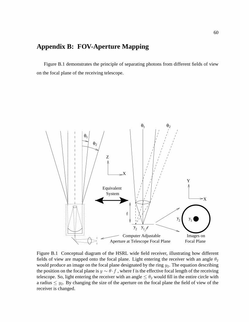
60

Appendix B: FOV-Aperture Mapping

Figure B.1 demonstrates the principle of separating photons from different fields of view

on the focal plane of the receiving telescope.

f

Z

X

y2

y1y2

y1

Equivalent System

Y

X

Computer Adjustable Aperture at Telescope Focal Plane

Images onFocal Plane

θ1 θ2

θ1

θ2

Figure B.1 Conceptual diagram of the HSRL wide field receiver, illustrating how differentfields of view are mapped onto the focal plane. Light entering the receiver with an angleθ2

would produce an image on the focal plane designated by the ringy2. The equation describingthe position on the focal plane isy ∼ θ ·f , where f is the effective focal length of the receivingtelescope. So, light entering the receiver with an angle≤ θ2 would fill in the entire circle witha radius≤ y2. By changing the size of the aperture on the focal plane the field of view of thereceiver is changed.