a theoretical analysis for tube bulge forming using

AIJSTPME (2012) 5(4): 7-20

7

A theoretical analysis for tube bulge forming using elastomer medium

Ramezani M. and Neitzert T.

Centre of Advanced Manufacturing Technologies (CAMTEC), School of Engineering, Auckland University of

Technology, Auckland, New Zealand

Abstract

A new theoretical model is presented in this paper for bulge forming of tubular components with solid bulging

mediums. The model is based on the results of the friction model which was developed previously by one of the

authors for rubber/metal contact and takes into account the effect of local contact conditions. FE simulations

using commercial software ABAQUS are carried out for an axisymmetric tube bulging operation using the

defined friction model. The comparisons of the results of the theoretical model and the FE simulations clearly

show that the newly developed theoretical model is suitable for predicting forming pressure and stress in the

tube. The effect of key process parameters such as the friction between the tube and the die, the tube initial

thickness and the length of the ealastomeric rod on the results are investigated using theoretical and FE

models.

Keywords: Finite element simulation; Friction; Theoretical analysis, Tube bulging.

1 Introduction

In recent years, tube bulge forming techniques have

been used in producing a wide range of tubular

components. This is mainly due to the quest to

decrease production costs and to optimize production

technology. This technique is used for producing

bicycle frame brackets from mild steel bulging and to

manufacture the rear axle castings for automobiles.

The process is also widely used in forming copper

pipe fittings for domestic water and gas supplies [1].

The bulge forming of pipes can be done by

implementing the internal hydrostatic pressure via a

medium. The pressure medium is usually a liquid

(hydraulic fluid or water) or solid elastomer (rubber

or polyurethane). By restraining the pipe in dies with

different geometries, components with desired shapes

can be produced. Excessive thinning due to the high

internal pressure is the main limitation of this

process. To overcome this problem, compressive

axial loading is applied to the end of the tube together

with the internal pressure. In the bulge forming of

tubes with solid medium, an elastomer rod inside the

tube applies lateral pressure to expand the tube

circumferentially, while simultaneous axial feeding

of the tube is secured by the frictional traction on the

tube as the elastomer rod deforms relative to the tube.

The use of elastomeric media has further advantages.

The need for an elaborate control system to co-

ordinate the axial compression with the hydraulic

pressure is eliminated. Frictional forces between the

tube and the elastomer are used to generate the axial

compression, and the flexible medium applies a

lateral pressure to the tube causing it to expand

within the die. Moreover, the friction acting on the

tube has an advantage in delaying the onset of tensile

instability. When bulging with solid medium, sealing

problems and the possibility of leakage of the high-

pressure liquid employed in hydraulic bulging are

eliminated. The cost of producing the component is

much less than using a specialized machine required

for hydraulic bulging. The need for the filling and

removal of oil or the cleaning of the bulged tube of

oil after forming is eliminated. The insertion of the

elastomer rod is both quick and convenient and the

rod can be re-used again [2].

Many experimental studies concerning bulge forming

are available in literature [3-4] and in recent years a

significant number of finite element simulation

studies have been detailed out [5-8]. Different

theoretical models have also been developed for the

process [9-11]. Mac Donald and Hashmi [5]

developed a three-dimensional simulation of the

Ramezani M. and Neitzert T. / AIJSTPME (2012) 5(4): 7-20

8

manufacture of cross-branch components using a

solid bulging medium. The effect of varying friction

between the bulging medium and the tube was

examined in their paper and the history of

development of the bulge and stress conditions in the

formed component were investigated.

Hwang and Lin [7] proposed a theoretical model to

examine the plastic deformation behavior of a thin-

walled tube during the bulge hydro-forming process

in an open die. They considered non-uniform

thinning in the free-bulged region and sticking

friction between the tube and die. The analysis was

followed by finite element simulation of the process

using DEFORM and the relationship between the

internal pressure and the bulge height of the tube was

achieved. Yang et al. [8] investigated the effect of the

loading path on the bulged shape and the wall

thickness distribution of the tube using theoretical

and FE models. Using their model, a reasonable

range of the loading path for the tube bulge hydro-

forming process was determined.

Thiruvarudchelvan [9, 10] developed a theoretical

model based on the experimental friction analysis

performed by Fakuda and Yamaguchi [12]. Using

this model he could determine the initial yield

pressure and the final forming pressure needed to

bulge a tube. Boumaiza et al. [11] discussed the

plastic instabilities of elasto–plastic tubes subject to

internal pressure and developed a local necking

criterion based on a modified Hill’s assumption for

localized necking. In all these studies, the FE and

theoretical analysis based on a comprehensive

analytical friction model which takes into account the

local contact condition have been missed.

Ramezani et al. [2] developed a friction model for

rubber-metal contact in tube bulge forming process

using solid medium. They showed in their paper that

the newly developed friction model is very effective

in producing reliable FE simulations compared to a

traditional Coulomb friction model. In the present

work, this friction model is used in theoretical

analysis of tube bulging process to examine its

efficacy in developing analytical models for rubber

forming processes. Based on the results of a friction

model developed by Ramezani et al. [2, 13] and an

analytical model developed by Thiruvarudchelvan

[9], an analytical analysis is performed for the case of

tube end bulging with polyurethane medium,

followed by finite element simulation of an

axisymmetric tube bulging operation using ABAQUS

software. To evaluate the influence of the new

friction model, theoretical and FE simulation results

have been compared with each other and with

experimental results from [4].

2 Static friction model

When two solids are squeezed together they will in

general not make atomic contact everywhere within

the apparent contact area and contact happens only on

peak asperities of surfaces [14]. To model the contact

between rough surfaces, it is necessary to determine

the contact parameters between the pair of asperities

carrying the load [15]. For two elastic spherical

asperities which are loaded by a normal force nF ,

Hertz theory [16] is the basic theory for specifying

the radius of the contact circle, the pressure and the

normal approach. For the case when a tangential

force tF is subsequently applied, the tangential

displacement of asperities and the shear stress within

the contact can be determined by Mindlin theory

[17]. He considered a stick region in the centre of

contact between a pair of asperities surrounded by an

annulus area of micro-slip across the edge of the

contact. Johnson [18] presented a solution for this

micro-slip region.

Rubber materials exhibit both elastic and viscous

resistance to deformation. The materials can retain

the recoverable (elastic) strain energy partially, but

they also dissipate energy if the deformation is

maintained [13]. Viscoelastic materials behavior can

be modeled using springs and dashpots connected in

series and/or in parallel. A dashpot is connected in

parallel with a spring in Figure 1. This is known as a

Voigt element. If deformed, the force in the spring is

assumed to be proportional to the elongation of the

assembly, and the force in the dashpot is assumed to

be proportional to the rate of elongation of the

assembly. In this model, if a sudden tensile force is

applied, some of the work performed in the assembly

is dissipated in the dashpot while the remainder is

stored in the spring.

A dashpot is connected in series with a spring is

shown in Figure 1(b). This is called a Maxwell

element. In this assembly, if a sudden tensile force is

applied, it is the same in both the spring and the

dashpot. The total displacement experienced by the

element is the sum of the displacements of the spring

and the dashpot. The response of rubber to changes in

stress or strain is actually a combination of elements


9

of both mechanical models (see, Figure 1(c)). The

response is always time-dependent and involves both

the elastic storage of energy and viscous loss.

The Standard Linear Solid (SLS) model (Figure 1(c))

gives a relatively good description of both stress

relaxation and creep behavior. Stress relaxation is the

time-dependent decrease in stress under constant

strain at constant temperature. For the SLS model the

generalized Hook’s equation can be written as

).( 21211 ggggg dd (1)

where 1g , 2g are the elasticity of springs, d is

the viscosity of the dashpot, is the strain and is

the stress.

By making the stress constant and equal to 0 in

Eq. (1) and solving the differential equation with

respect to the strain , we arrive at the creep

compliance function )(t as follows:

)]exp(1[11)(

)(2210 T

t

gg

tt

(2)

where

22

gT d is the retardation time.

Similarly, the stress relaxation function )(t can be

obtained by taking the strain constant and equal to

0 in Eq. (1), resulting in

)]exp([)(

)(2

1221

1

0 T

tgg

gg

gtt

(3)

where )( 21

2gg

T d

is the retardation time.

Surface roughness can be modeled as a composed set

of spherical asperities which have the same radius

and their heights following a statistical distribution,

as for instance a Gaussian distribution (see, Figure 2).

Three parameters are commonly used to describe a

random rough surfaces model. The statistical

parameters of the asperities are: the average asperity

radius (spherical shaped asperities), the asperity

density n , and the standard deviation of the asperity

heights s . According to experiments reported by

Greenwood and Williamson [19] most surfaces show

a value in the range of 0.03-0.05 for the product

sn .

Hui et al. [20] developed a theory for viscoelastic-

rigid contacts under several loading conditions such

as constant load test, load relaxation test and constant

displacement rate test. In this theory, an

exponentially distribution of asperities is considered

and then an analytical solution is developed for the

real contact area and the total normal load. In this

paper, the case of a viscoelastic rough surface which

is normally loaded against a rigid surface is

considered.

2.1 Normal loading of viscoelastic/rigid multi-

asperity contact

For a certain separation h the number of asperities in

contact, the real contact area and the total load carried

by the asperities can be calculated using the

following equations. The number of asperities in

contact at a certain separation is given by

h

nc sdsnAn )( (4)

where nA denotes the nominal contact area,

sss / is the normalized asperity height,

shh / is the normalized separation, and )(s

is the normalized Gaussian height distribution which

can be obtained as

2

2

2

1)(

s

es

(5)

Then, the real contact area is given by:

h

snr dsshsnAA )()( (6)

The total normal load can be obtained as the sum of

all normal loads carried by the asperities in contact.

sdshst

nAF

h

snn )()()(

1

3

8 2

3

2

3

2

1

(7)


10

2.2 Tangential loading of viscoelastic/rigid multi-

asperity contact

Considering the multi-asperity contact introduced in

Section 2.1 to be subsequently loaded by an

increasing tangential load, an approach is presented

in this section for a viscoelastic rough surface pressed

against a rigid flat.

At a certain separation and for a tangential load

smaller than the force necessary to initiate macro-

sliding, so-called maximum static friction force, the

multi-contact interface will be composed of micro-

contacts which are in the partially-slip regime and

micro-contacts which are totally sliding. Macro-

sliding will occur if all contacting asperities are in the

fully sliding regime [17].

A condition has been set for an elastic multi-contact

interface by Bureau et al. [21] which provides a

critical asperity height above which the micro-

contacts are partially sliding. In their approach, a

constant local coefficient of friction is considered for

all micro-contacts. Using Bureau method, a critical

asperity height for a viscoelastic multi-contact

interface can be derived.

]).

1(1[)2()()( 3

2

n

tntv

F

Ftt

(8)

where tv is the preliminary displacement; is the

Poisson’s ratio; and is the local coefficient of

static friction. Rearranging the factors in Eq. (8), we

arrive at:

3

2

).

1()2()(

)(1

n

t

n

tv

F

F

t

t

(9)

The right-hand side of Eq. (9) is a positive real

number for nt FF . , thus:

)()2(

)(t

tn

tv

(10)

The indentation depth of the asperity n can be

replaced by )( hz . Then, the inequality (10)

becomes

ht

z tv

)2(

)(

(11)

From Eq. (11) it can be inferred that the asperities

which have the height

ht

s tvc

)2(

)(

(12)

are in the fully sliding regime because they carry a

tangential force which is equal to or larger than the

maximum static friction force. The micro-contacts of

which heights satisfy the relation csz are in the

partially-slip regime.

The total tangential load carried by the multi-contact

interface can be written as:

slipstickt FFF (13)

where stickF component is calculated as the sum of

all tangential loads carried by the micro-contacts

which are not fully sliding. That means that their

contact areas are composed of stick and slip regions.

Deladi [22] presented the following equation for

stickF component:

sdhs

shs

tnAtF

cs s

t

snstick

2

3

2

3

2

1

2

3

)()2(11)()(

)(

1

3

8)(

(14)

The slipF component is taken as the sum of all

tangential loads carried by the micro-contacts which

are fully sliding and is calculated with equation

sdc

s

h

shs

tsn

nAt

slipF

)(2

3

)(

2

1

)(

1

3

82

3)(

(15)

Having obtained the tangential load carried by the

multi-contact interface, the maximum force required

to initiate macro-sliding (or maximum static friction

force) can be determined as the sum of all tangential

loads causing gross sliding of all micro-contacts [22].

When this condition is obeyed, the partially sliding


11

component stickF becomes zero and the condition

can be written as:

0max

stick

Fifslip

Fst

F (16)

So, the static coefficient of friction can be

calculated as:

nF

stFs

max (17)

By giving the micro-geometry, the nominal area of

contact and the material properties, the real area of

contact, rA and the normalized separation, h can be

obtained from Eqs. (6) and (7). Next, assuming a

tangential displacement, the critical height, cs can

be calculated from Eq. (12). Then, the tangential

loads carried by each micro-contact are obtained

from Eqs. (14) and (15). If the partially stick

component of the tangential force is not zero, the

tangential displacement should be increased until all

micro-contacts are fully sliding. This maximum

tangential displacement corresponding to the

occurrence of macro-sliding is taken as the global

limiting displacement. At this stage, the maximum

static friction force is reached and so, the static

coefficient of friction is determined from Eq. (17).

Figure 1: Mechanical models representing the

response of viscoelastic materials: (a) Voigt model,

(b) Maxwell model, (c) SLS model.

Figure 2: Contact model of rough surfaces.

2.3 Calculation of friction coefficient

An Alicona imaging infinite focus microscope (IFM

2.1) was used to measure the surface parameters of

polyurethane. Surface parameters in terms of density

of asperity n , mean radius of asperity , and

standard deviation of the asperity heights s are the

input parameters of the friction model. Figure 3

shows the roughness profile along a selected line in

the surface. The geometrical parameters mentioned

above can be obtained by these measurements using

the Alicona microscope.

The viscoelastic material parameters in terms of

spring elasticity 21, gg and dashpot viscosity d of

the SLS model are the other input parameters of the

friction model. The values of viscoelastic material

parameters used in the calculations of the friction

model are obtained from a stress relaxation test of

rubber. In a stress relaxation test a compressive strain

at a constant rate within a very brief period of time is

applied on an unconstrained cylinder and the stress

required maintaining the compressive strain is

recorded in time. The test is performed according to

ASTM D 6048 standard. Stress relaxation modulus as

a function of time (see, Eq. 3) for polyurethane of

Shore hardness A 95 is shown in Figure 4. According

to Eqs. (2) and (3), for 0t we obtain

11)0()0( g and for t we have

21

211

.)()(

gg

gg . The values of input

parameters for calculation of the coefficient of

friction as a function of contact pressure are

presented in Table 1.

Figure 3: Roughness profile for polyurethane.

Using the values of parameters in Table 1 as input

values for the friction model presented in Section 2,

we calculated the coefficient of friction between

polyurethane and copper tube as a function of contact

pressure (see, Figure 5). It can be seen from Figure 5


12

that an increase in contact pressure results in decrease

in coefficient of friction. At low pressures this

decrease is more significant than at higher loads

when the coefficient of friction reaches a quite stable

level. This is comparable to the observation made by

Benabdallah [23] where experimental work on some

thermoplastics against steel and aluminum showed

similar effect.

Figure 4: Stress relaxation modulus as a function of

time for polyurethane rubber.

Figure 5: Coefficient of friction (for polyurethane/

copper contact) as a function of contact pressure.

The physical explanation for the increasing friction

coefficient at lower pressures is that the effect of the

adhesion force becomes more significant at lower

normal loads [24]. High adhesion force decreases the

separation h , at a given normal load and brings more

asperities into contact especially when the normal

load is small, enabling support for larger tangential

load, and hence, the friction force and friction

coefficient increase with decreasing normal load.

From Figure 5 the following equation for the

variation of coefficient of friction s with pressure

P is curve-fitted.

22.0695.0 Ps (18)

Table 1: Values of the input parameters for friction

model.

Parameters Values

n )( 2m 11107.2

)( m 542.0

s )( m

28.0

1g )(Pa

71030.8

2g )(Pa 81089.1

d ).( sPa 91068.2

4.0

3 Theoretical model

The schematic of tube bulge forming is shown in

Figure 6. As can be seen in the figure, the tube and

the polyurethane rod are divided into two zones (i.e.

0-1 and 1-2) to simplify the theoretical analysis. The

tube is in full contact with the die wall in zone 0-1

and there is no plastic deformation of tube in this

region. However, the tube is not constrained

circumferentially in zones 1-2 and can deform

plastically until taking the shape of the die. The

theoretical model presented in this section is based on

the work of Thiruvarudchelvan [9]. Mathematical

formulations for the pressure in the polyurethane rod

and stress components in the tube are developed for

each zone and are presented below.

Zone 0-1:

According to Figure 6, the equilibrium equation for

polyurethane rod at zone 0-1 can be expressed as

xdpd

p s d4

d2

(19)


13

Substituting Eq. (18) into Eq. (19) and simplifying

the result, we arrive at

xd

pp d695.04

d78.0

(20)

By integrating Eq. (20), we will have

Cd

xC

d

xp 612.0695.088.022.0

(21)

According to Figure 6 at 0x we have 0pp

and so Cp 22.00 . Therefore

22.0 22.00 612.0

d

xpp (22)

Figure 6: Schematic of tube bulge forming process.

On the other hand, the compressive axial load on the

tube exerted by the polyurethane frictional force can

be expressed as

)(4

0

2

ppd

Fx

(23)

As the tube is dragged to the die surface, the

frictional force exerted on the tube from the die is

xd

xpdxdpF

xx

F d612.0

d0

22.0 22.000

0

0

(24)

Integrating Eq. (24) leads to

22.122.100

22.1612.0

22.0pp

ddFF

(25)

where 0 is the coefficient of friction between the

die and the tube. The axial compressive stress and the

hoop stress on the tube wall in zone 0-1 can now be

easily derived from Eqs. (22), (23) and (25) by using

the following equations:

22.122.1

00

22.0 22.0

00

295.0

612.0

4

ppT

d

d

xpp

T

d

Td

FF Fxx

(26)

22.0 22.0

0

612.0

22 d

xp

T

d

T

dp (27)

As the tube is completely surrounded by the die wall

at zone 0-1, the hoop stress is small and may be

neglected. For this region and by neglecting the

lateral pressure p , the Tresca yield criterion is

01.1 x , where 0 is the initial yield

stress of the tube material. Thus

0

22.122.1

00

22.0 22.0

00

1.1295.0

)612.0

(4

ppT

d

d

xpp

T

dx

(28)

Zone 1-2:

The axial equilibrium equation for the polyurethane

rod at zone 1-2 can be expressed as

)cos(sincos

d

4)d(

4

)d( 22

s

xpD

pD

PpDD

(29)

By neglecting higher order terms of Eq. (29) and

rearranging the equation, we have


14

)(tantan2

d4)dd2(

DppDDp (30)

Considering tan2/dd Dx , we have

cot39.1

d

cot2

dd78.0p

p

p

p

D

D

s

(31)

Integrating Eq. (31) leads to

0cot39.111

50ln 22.0

CpD

(32)

According to Figure 6 at dD we have 1pp

and so Cpd

22.0

1cot

27.3ln

. Therefore

22.0 22.01 cotln306.0

d

Dpp (33)

Neglecting the effect of bending at point 1, the

equilibrium equation normal to the conical surface of

the tube at zone 1-2 is

T

pp

r

d

cos (34)

where is the tensile hoop stress. Assuming

constant thickness, the equilibrium equation along the

axis of the tube is

cotcot)(d

)(dcos 0 dsd pprpp

r

rT

(35)

Combining Eqs. (34) and (35) leads to

rT

pp

rr

ds dcos

cot)(

dd

0

(36)

where and are tensile and compressive

stresses respectively. Using the modified Tresca yield

criterion m 1.1 and combining Eqs.

(34) and (36) lead to

rppT

r

r

r

rm

d)695.0(eccos

d)1cot(1.1

dcotd

0

78.0

00

(37)

where m is the average yield stress of the tube

material. By integrating and manipulating Eq. (37),

we arrive at the following expression for the

compressive meridian stress in section 2 ( 2rr ):

rrr

rp

DT

rrr

rp

DT

D

d

D

d

r

r

r

r

m

dlncot306.0)2/(

eccos

dlncot306.0)2/(

eccos695.0

1cot

1cot1.1

)cot(

55.4

1

22.0

1)cot(

0

)cot(

55.3

1

22.0

1)cot(

)cot(

0

01

)cot(

2

0

2

1

0

0

2

1

0

00

(38)

Calculation procedure:

From the above calculations, the pressures at sections

1 and 2 are given by Eqs. (22) and (33), respectively.

22.0 22.012

22.0 122.001

cotln306.0

612.0

d

Dpp

d

Lpp

(39)

Also, the compressive meridian stresses at sections 1

and 2 can be achieved by Eqs. (26) and (38),

respectively.

22.11

22.10

0101

295.0

4pp

T

dpp

T

d

(40)

rrr

rp

DT

rrr

rp

DT

D

d

D

d

r

r

r

r

m

dlncot306.0)2/(

eccos

dlncot306.0)2/(

eccos695.0

1cot

1cot1.1

)cot(

55.4

1

22.01)cot(

0

)cot(

55.3

1

22.01)cot(

)cot(

0

01

)cot(

2

0

2

1

0

0

2

1

0

00

(41)

The initial pressure exerted on the top of the

polyurethane rod to bulge the tube, 0p can be

obtained from FE simulations and subsequently, the

values of 21 , pp and 21 , can be calculated

using Eqs. (39-41).


15

4 Finite element simulation

Numerical studies were carried out to reveal the

deformation pattern of the tube and to verify the

theoretical analysis. A range of forming parameters

can be used in the finite element simulations and the

optimal values can be predicted at low CPU cost.

ABAQUS finite element code was used to simulate

the process and predict the material deformation

during forming. Due to the axisymmetric character of

the forming, only a 2-D model was used to reduce

computation time. Figure 7 shows the shape at the

last stage of the tube bulging using a solid bulging

medium. A polyurethane rod of Shore Hardness 95A

and diameter 38mm was used to bulge an annealed

copper tube of diameter 42mm and wall thickness of

1.2mm. The bottom plate of the die was not modeled,

instead the nodes at the bottom of die, tube and

flexible medium were constrained in the appropriate

directions to simulate the presence of the die bottom

plate.

Figure 7: FE simulation of the process at the last

stage of bulge forming.

Die tool material was assumed to be steel, and the

tube was modeled using CAX4R (a 4-node bilinear

axisymmetric quadrilateral, reduced integration,

hourglass control) elements. The polyurthane rod was

modeled using CAX4RH elements. Penalty contact

interfaces were used to enforce the intermittent

contact and the sliding boundary condition between

the blank and the tooling elements. The Coulomb

friction model with various values of coefficient of

friction is used for contact surfaces between the tube

and the metallic die. The coefficient of friction

between the polyurethane and the tube changes with

contact pressure based on the model presented in

section 2. The contact pressure dependent

coefficients of friction are implemented into the

model through the contact property option of the

ABAQUS program. This option is used to introduce

friction properties into the mechanical surface

interaction models.

The simulation begins with the tube in contact with

the die and the polyurethane rod. The flexible rod

then moves down to bulge the tube. The interface

between the die and the tube, and between the tube

and the flexible rod are modeled using an automatic

surface to surface contact algorithm. The forming

loads were applied on the polyurethane rod in terms

of displacements on the top surface of the rod. The

displacement was assigned to be equal to the

displacement of the rod measured during the

experimental tests performed by Girard et al. [4].

The constitutive behavior of the tube is described by

an elastic–plastic model. For the elastic part, Young's

modulus of 110GPa and Poisson's ratio of 0.343 is

used. For the plastic part, the hardening model is

assumed to be isotropic described by the power law

approach:

nK (42)

where is the true stress (MPa), is the total true

strain (dimensionless), K is the strength coefficient

(MPa) and n is the strain-hardening exponent

(dimensionless). For the annealed copper in this

research, MPaK 530 and 44.0n are being

used and the average yield stress of the annealed

copper is MPam 97 .

Rubber is made of isotropic, non-linear, hyper-

elastic, incompressible, strain-history-independent

material. Hyper-elastic materials are described in

terms of a strain energy potential W which defines

the strain energy stored in the material per unit of

reference volume (volume in the initial configuration)

as a function of the strain at that point in the material


16

[25]. Among several forms of strain energy potentials

available in ABAQUS, Ogden (N=3) strain energy

[26] is used for rubber modeling. The Ogden material

model has previously been used with success to

predict the behavior of hyper-elastic materials at high

strain rates (see, e.g. [27]). The form of the Ogden

strain energy potential is:

ijij

W

(43)

iel

i

N

i

i

iN

i

JD

W iii

2

1

32121

)1(1

)3(2

(44)

where W is the strain energy per unit of reference

volume;

i are the deviatoric principal stretches

which can be defined by ii J 3/1 ; i are the

principal stretches; J is the total volume ratio; elJ

is the elastic volume ratio; and i , i and iD are

temperature-dependent Ogden constants.

Compressibility can be defined by specifying nonzero

values for iD , by setting the Poisson's ratio to a

value less than 0.5, or by providing test data that

characterize the compressibility. We assumed a fully

incompressible behavior for rubber with

4997.0 and iD

equal to zero and so the

second expression in Eq. (44) can be eliminated. To

determine the strain energy density W, ABAQUS

uses a least-squares fitting algorithm to evaluate the

Ogden constants automatically from experimental

data.

5 Results and discussions

To validate the FE model developed in Section 4, the

final thickness of the tube after bulging is compared

with experimental results presented by Girard et al.

[4] and is shown in Figure 8. As demonstrated in the

figure, the thickness distribution obtained from the

FE model and the experiments agree very well with

each other with the error less than 6%. As shown in

the figure, the maximum thinning happens at the end

of the tube, where the tube has the maximum

expansion. The undeformed part of the tube does not

show any reduction in thickness.

The pressure 0P at the top of the polyurethane rod

obtained from FE simulations with different values of

coefficient of friction between the die and the tube is

shown in Figure 9. As can be seen in the figure,

higher pressures are needed for bulging with higher

friction coefficients to overcome the frictional

resistance between the die and the tube.

Figure 8: Thickness distribution of the bulged tube

obtained from FE simulations.

Figure 9: Pressure at the top of the polyurethane rod

obtained from FE simulations.

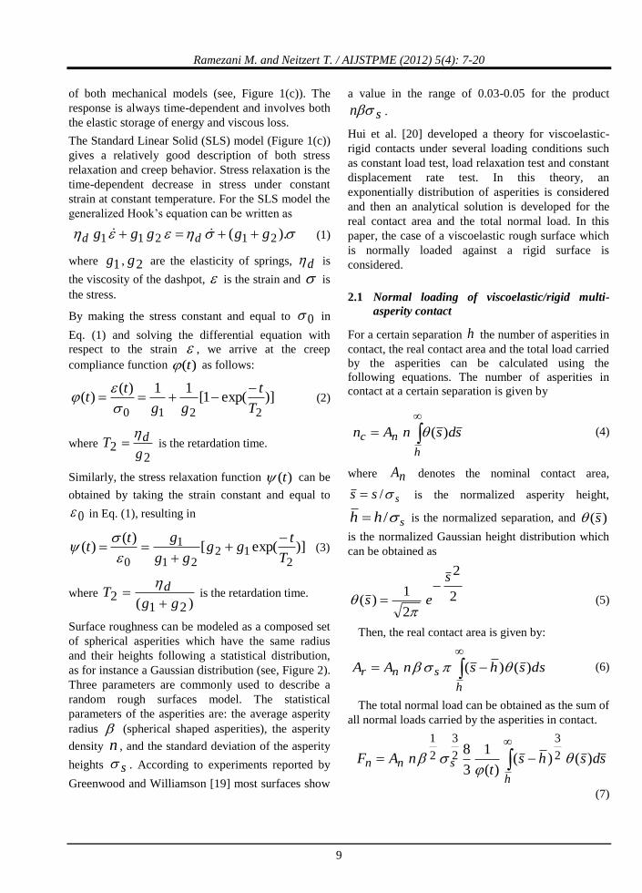
The variations of pressures at points 1 and 2

(see Figure 6) of the rod are illustrated in Figures 10

and 11. The values of 1P and 2P are calculated using

Eq. (39). According to the figures, the results of FE

simulations and the theoretical model correlate with

each other. The maximum error for predicting 1P is


17

4.6% which happens at the coefficient of friction of

0.1. The error increases to 4.9% for prediction of 2P .

Figure 10: Variation of 1P with coefficient of

friction.

Figure 11: Variation of 2P with coefficient of

friction.

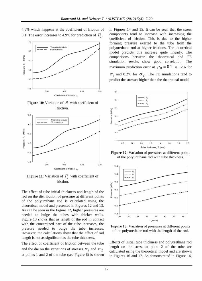
The effect of tube initial thickness and length of the

rod on the distribution of pressure at different points

of the polyurethane rod is calculated using the

theoretical model and presented in Figures 12 and 13.

As can be seen in the Figure 12, higher pressures are

needed to bulge the tubes with thicker walls.

Figure 13 shows that as length of the rod in contact

with the constrained part of the tube increases, the

pressure needed to bulge the tube increases.

However, the calculations show that the effect of rod

length is not as significant as the tube thickness.

The effect of coefficient of friction between the tube

and the die on the variations of stresses 1 and 2

at points 1 and 2 of the tube (see Figure 6) is shown

in Figures 14 and 15. It can be seen that the stress

components tend to increase with increasing the

coefficient of friction. This is due to the higher

forming pressure exerted to the tube from the

polyurethane rod at higher frictions. The theoretical

model predicts this increase quite linearly. The

comparisons between the theoretical and FE

simulation results show good correlation. The

maximum prediction error at 2.00 is 12% for

1 and 8.2% for 2 . The FE simulations tend to

predict the stresses higher than the theoretical model.

Figure 12: Variation of pressures at different points

of the polyurethane rod with tube thickness.

Figure 13: Variation of pressures at different points

of the polyurethane rod with the length of the rod.

Effects of initial tube thickness and polyurethane rod

length on the stress at point 2 of the tube are

calculated using the theoretical model and are shown

in Figures 16 and 17. As demonstrated in Figure 16,


18

the stress at point 2 increases sharply with decreasing

the initial tube thickness which makes it difficult to

bulge very thin tubes. According to Figure 17, the

increase in the rod length does not have a remarkable

effect on the stress at point 2.

Figure 14: Variation of stress 1 with coefficient of

friction.

Figure 15: Variation of stress 2 with coefficient of

friction.

The history of radial stress at points 1 and 2 during

the FE simulation is shown in Figure 18. As shown in

the figure, the compressive radial stress increases

constantly during the process and makes it possible to

expand and bulge the tube end. The values of stresses

at points 1 and 2 are quite similar which is due to the

hydrostatic nature of the bulge forming using an

elastomer bulging medium. The variation of axial

stress at points 1 and 2 of the tube with simulation

time is shown in Figure 19. As can be seen in the

figure, the axial stresses increase with time, however

there is a sharp decrease in axial stress at point 1 at

the end stages of the bulge forming process.

Figure 16: Effect of initial tube thickness on

stress 2 .

Figure 17: Effect of polyurethane rod length on

stress 2 .

Figure 18: Radial stress history at point 1 ad 2 of the

tube during bulging simulation.


19

Figure 19: Axial stress history at point 1 ad 2 of the

tube during bulging simulation.

6 Conclusions

In this paper bulge forming of tubular components

was investigated using an analytical model and FE

simulations. A new friction model based on local

contact conditions was used in the FE simulation of

the process and based on the results of this friction

model, a theoretical model for bulge forming was

developed. The main conclusions of this research are

as follows:

An increase in contact pressure results in decrease

in coefficient of friction between rubber and

metal. The coefficient of friction reaches a nearly

constant value at higher normal pressures.

Higher pressures are needed to bulge the tubes

with thicker walls. The stress at the end of the

tube increases sharply with decreasing the initial

thickness of the tube, which may cause rupture at

the end of the tubes with very thin walls.

The effect of the length of the elastomeric rod on

the pressure and stress distributions is negligible.

Compressive axial and radial stresses at the tube

increase constantly during the process which

makes it possible to bulge the tube.

References

[1] Mac Donald BJ, Hashmi MSJ (2002) Near-net-

shape manufacture of engineering components

using bulge-forming processes: a review. J

Mater Process Technol 120:341–347.

[2] Ramezani M, Ripin ZM, Ahmad R (2009) A

static friction model for tube bulge forming

using a solid bulging medium. Int. J. Adv.

Manuf. Tech. 43 (3–4):238–247.

[3] Kim J, Kim SW, Park HJ, Kang BS (2006) A

prediction of bursting failure in tube

hydroforming process based on plastic

instability. Int J Adv Manuf Technol 27:518–

524.

[4] Girard AC, Grenier YJ, Mac Donald BJ (2006)

Numerical simulation of axisymmetric tube

bulging using a urethane rod. J Mater Process

Technol 172:346–355.

[5] Mac Donald BJ, Hashmi MSJ (2001) Three-

dimensional finite element simulation of bulge

forming using a solid bulging medium. Finite

Elem Anal Des 37:107–116.

[6] Pipan J, Kosel F (2002) Numerical simulation

of rotational symmetric tube bulging with inside

pressure and axial compression. Int J Mech Sci

44:645–664.

[7] Hwang YM, Lin YK (2002) Analysis and finite

element simulation of the tube bulge

hydroforming process. J Mater Process Technol

125–126:821–825.

[8] Yang B, Zhang WG, Li SH (2006) Analysis and

finite element simulation of the tube bulge

hydroforming process. Int J Adv Manuf

Technol 29 (5):453–458.

[9] Thiruvarudchelvan S (1994) A theory for the

bulging of aluminum tubes using a urethane

rod. J Mater Process Technol 41:311–330.

[10] Thiruvarudchelvan S (1994) A theory for initial

yield conditions in tube bulging with a urethane

rod. J Mater Process Technol 42:61–74.

[11] Boumaiza S, Cordebois JP, Brunet M, Nefussi

G (2006) Analytical and numerical study on

plastic instabilities for axisymmetric tube

bulging. Int J Mech Sci 48:674–682.

[12] Fukuda M, Yamaguchi K (1974) On the

coefficient of friction between rubber and metal

under high pressure. Bulletin of JSME 17

(103):157–164.

[13] Ramezani M, Ripin ZM, Ahmad R (2009)

Computer aided modelling of friction in rubber-

pad forming process. J Mater Process Technol

209 (10):4925-4934.


Modelling of kinetic friction in V-bending of

ultra-high-strength steel sheets. Int J Adv

Manuf Technol 46 (1-4):101-110.

[15] Ramezani M, Ripin ZM (2010) A friction

model for dry contacts during metal-forming

processes. Int J Adv Manuf Technol 51

(1-4):93-102.

http://www.scopus.com/search/submit/author.url?author=Ramezani%2c+M.&origin=resultslist&authorId=24081569700&src=s

http://www.scopus.com/search/submit/author.url?author=Ripin%2c+Z.M.&origin=resultslist&authorId=7801694840&src=s

http://www.scopus.com/search/submit/author.url?author=Ahmad%2c+R.&origin=resultslist&authorId=24079897000&src=s




http://www.sciencedirect.com/science/journal/09240136




20

[16] Hertz H (1882) Über die Berührung fester

elastischer Körper. J. Reine. Angew. Math.

92:156–171.

[17] Mindlin RD (1949) Compliance of elastic

bodies in contact. ASME J. Appl. Mech. 16:

259–268.

[18] Johnson KL (1985) Contact mechanics.

Cambridge: Cambridge University Press.

[19] Greenwood JA, Williamson JBP (1966) Contact

of nominally flat surfaces. Proc. Roy. Soc.

London, A 295:300–319.

[20] Hui CY, Lin YY, Baney JM (2000) The

mechanics of tack: viscoelastic contact on a

rough surface. J Polym Sci, B: Polymer

Physics, 38:1485–1495.

[21] Bureau L, Caroli C, Baumberger T (2003)

Elasticity and onset of frictional dissipation at a

non-sliding multi-contact interface. Proc. Roy.

Soc. London, A 459, 1183:27871–2805.

[22] Deladi EL (2006) Static friction in rubber–

metal contacts with application to rubber pad

forming processes. PhD thesis, University of

Twente, The Netherlands.

[23] Benabdallah HS (2007) Static friction

coefficient of some plastics against steel and

aluminum under different contact conditions.

Tribol. Int. 40:64–73.

[24] Yu N, Pergande SR, Polycarpou AA (2004)

Static friction model for rough surfaces with

asymmetric distribution of asperity heights.

ASME J Tribol 126:626–629.


Numerical simulation of sheet stamping process

using flexible punch. Proc. IMechE, B: J. Eng.

Manuf. 223 (7):829-840.

[26] Ogden RW (1972) Large deformation isotropic

elasticity–on the correlation of theory and

experiment for incompressible rubberlike

solids. Proc. Roy. Soc. London, A 326:565-84.

[27] Ramezani M, Ripin ZM (2010) Combined

experimental and numerical analysis of bulge

test at high strain rates using split Hopkinson

pressure bar apparatus. J. Mater. Process. Tech.

210 (8):1061-1069.




http://www.scopus.com/source/sourceInfo.url?sourceId=20406&origin=resultslist

http://www.scopus.com/source/sourceInfo.url?sourceId=20406&origin=resultslist



http://www.sciencedirect.com/science/journal/09240136

a theoretical analysis for tube bulge forming using

Documents