a theoretical earth resistivity study with …
TRANSCRIPT

A THEORETICAL EARTH RESISTIVITY STUDY
WITH APPLICATIONS ON THE
LLANO ESTACADO
by
RUSSELL A. BLUMENTRITT, B. S.
A THESIS
IN
GEOLOGY
Submitted to the Graduate Faculty of Texas Technological College in Partial Fulfillment of the Requirements for
the Degree of
MASTER OF SCIENCE
August, 1969
r3 / ^^^
/Jo Cop'
9 '
IL ABSTRACT
Mathematical model calculations and field resistivity measure
ments related to ground-water investigations on the Llano Estacado
were made.
The original potential function equations by Ehrenburg and Watson
were extended to eleven parallel layers (ten layers and a half space)
to represent a horizontally stratified earth. From these equations
a computer program was written to calculate apparent resistivities
for the Wenner configuration. The properties of this computer program
and related plot subroutines are described.
Electrical resistivities on the Llano Estacado were determined
from available electric logs and surface resistivity measurements in
outcrop areas. These regional resistivities were used to represent
various earth models for the calculation of apparent resistivity
curves by digital computer.
A surface resistivity survey covering 150 square miles was car
ried out in the Yellow House Canyon area. The interpretation was made
from an isoresistivity map, resistivity profiles and sounding data.
A theoretical formation resistivity analysis, electrical interval logs
from surface data and sounding curves computed from an electric log
were also included in the area study.
A brief review of the history, applied surveys in the Western
hemisphere and theory of the surface resistivity method are also pre
sented. A catalogue of 462 apparent resistivity curves is included
in the appendix.
ii

ACKNOWLEDGMENTS
To the many people who helped make this study possible, my
sincere appreciation. In particular, I wish to express my gratitude
to:
Dr. John J. Dowling, for his suggestion of the original problem.
Without his sincere interest and boundless patience this study would
not have been possible.
Dr. William D. Miller, for his helpful criticism and suggestions.
Dr. George S. Innis, for the invaluable computer facilities and
services made available.
Mrs. Sandy Struve, for typing the manuscript.
My parents, Mr. and Mrs. S. A. Blumentritt, for their encourage
ment and aid during this study.
Hi

TABLE OF CONTENTS
ABSTRACT ii
ACKNOWLEDGMENTS iii
LIST OF ILLUSTRATIONS vii
I. INTRODUCTION 1
Electrical Methods of Exploration 1
Purpose 1
Previous Work 3
History 3
II. CASE HISTORIES 5
Salt-Water Boundaries 5
Pollution Investigations 5
Surveys in Illinois 6
Water Study in Jamaica 6
Arid Region Surveys 6
Location for Ground-Water Recharge Facilities. . . . 7
III. SURFACE RESISTIVITY METHOD 8
Theory of Current Flow 8
Resistivities of Sedimentary Rocks 9
Anisotropy 10
Electrode Arrangements to Measure Earth
Resistivities 11
Expression for Two Horizontal Layers 13
Multi-Layer Developments 17
Approximation and Direct Methods of Calculation
for a Small Number of Layers 18 iv

V
Standard Curve Compilations 18
IV. A RESISTIVITY COMPUTATION METHOD FOR LAYERED EARTH
MODELS 20
Original Derivation by Ehrenburg and Watson 20
Extension of Ehrenburg and Watson's Formulae . . . . 21
Determination of Reflection Combinations 21
Formulae for Electric Image Poles 23
V. SURFACE RESISTIVITY PROGRAM 26
Convergence Properties 27
Subroutines 33
Plot Subroutine No. 1 33
Plot Subroutine No. 2 34
VI. SUMMARY OF LLANO ESTACADO GEOLOGY AND HYDROLOGY . . . . 40
Geology 40
Hydrology 41
VII. DETERMINATION OF ELECTRICAL RESISTIVITIES ON THE
LLANO ESTACADO 42
Information from Electric Logs 42
Information from Surface Resistivity Measurements. . 43
VIII. PARAMETERS FOR MASTER CURVE COMPILATIONS 44
IX. CATALOGUE OF APPARENT RESISTIVITY CURVES 46
Description 46
Accuracy 46
X. APPARENT RESISTIVITY CURVES FOR THE WENNER ARRAY. . . . 48
XI. APPLIED SURVEY IN THE YELLOW HOUSE CANYON AREA 55
Geography 55
Field Survey 55

VI
Measurement Procedures 56
Reading Accuracy 57
Determination of Lateral Variations 58
Geology and Ground Water 58
Triassic System 58
Cretaceous System 58
Tertiary System 59
Quaternary System 59
Interpretation 60
Isoresistivity Map 60
Resistivity Profiles - Line A-A' 64
Sounding Curves - Line B-B* 68
Electric Log 74
XII. SUMMARY AND CONCLUSIONS 77
Theory and Computer Programming 77
Model Studies and Apparent Resistivity Curves. . . . 77
Survey in the Yellow House Canyon Area 78
General Discussion 79
Success of Surface Resistivity Measurements 80
LIST OF REFERENCES 81
APPENDIX 85

LIST OF ILLUSTRATIONS
Figures
Figure 1. Index map showing location of the Llano Estacado
and Yellow House Canyon area 2
Figure 2. Wenner configuration 12
Figure 3. Common in-line electrode arrangements for surface resistivity measurements 14
Figure 4. Positions of near images due to a source and
sink 15
Figure 5. Nomenclature for layered earth model 22
Figure 6. Q(N) coefficient pattern for model S 28
Figure 7. Q(N) coefficient pattern for model T 29
Figure 8. Q(N) coefficient pattern for model U 30
Figure 9. Q(N) coefficient pattern for model V 31
Figure 10. Layered models (part a) for x-y plot 36
Figure 11. Layered models (part b) for x-y plot 37
Figure 12. Tabulations of electrode spacings versus apparent
resistivities for x-y plot 38
Figure 13. Representative x-y plot by computer 39
Figure 14. Descending (A) and ascending (B) curves 49
Figure 15. Minimum (A) and maximum (B) curves 50
Figure 16. Double-descending (A) and double-ascending (B) curves 51
Figure 17. Descending double-ascending (A) and ascending
double-descending (B) curves 52
Plates
Plate I. Yellow House Canyon Area-Isoresistivity Map . . . 61
Plate II. Resistivity Profiles 65 • *
Vll

Vlll
Plate III. Field Sounding Curves with Computed Models. . . . 69
Plate IV. Electrical Log and Computed Sounding Curves . . . 75

CHAPTER I
INTRODUCTION
Electrical Methods of Exploration
The electrical properties of the subsurface can be examined ei
ther by electric or electromagnetic procedures. The three electrical
methods are (1) spontaneous- or self-potential (SP), (2) induced po
larization (IR) and (3) geoelectric or electrical resistivity (ER) .
The spontaneous-potential technique measures natural potential fields
in the earth. In the induced polarization method an artificial field
is applied and the earth response is measured. The electrical re
sistivity method is based on the application of a direct, commutated
or low frequency current into the ground. Measurement of the resulting
potentials at the surface enables one to determine the distribution
of the electrical resistivity in the subsurface.
Purpose
The purpose of this thesis is to provide a theoretical study with
applications of earth resistivity methods on the Llano Estacado
(Figure 1) by the following:
1. Extend existing equations for mathematical models which would include sufficient layers to realistically represent the geology of the Llano Estacado.
2. Based on the above mathematical denotations, write a computer program that will calculate standard graphs for resistivity prospecting.
3. Prepare an assemblage of master electrical resistivity curves which could be used to interpret field measurements .

YELLOW HOUSE CANYON AREA
33**55'
ss'so'
33** 45'
SCALE -M ILES
Figure 1. Index map showing location of the Llano Estacado and Yello^: House Canvon area

4. Apply the surface resistivity method to a diversified ground-water study in a local area.
Previous Work
An extensive literature survey was not a goal of this study, but
it was necessary to consult numerous sources not included in the List
of References. An extensive bibliography on resistivity methods can
be found in the publication by Van Nostrand and Cook (1966).
Numerous papers have been written on geophysical techniques re
lated to geological and hydrological studies in ground water. Ex
periments using shallow geophysical methods have been carried out on
the Llano Estacado, but these results were not available.
Textbooks on modern applied geophysics do not place much emphasis
on the surface resistivity method; therefore, a brief review of this
method is worthwhile.
History
As early as 1720 Gray and Wheeler made electrical studies of
rocks and listed their conductivities. Electrical prospecting meth
ods have grown from Fox's investigations of natural earth currents
through Schlumberger's use of artificial field forces from 1912-1914.
In 1912 Wenner stated the theorem of reciprocity with regard to four
electrodes and later calculated apparent resistivities by passing a
current between two electrodes and measuring the potential between
two auxiliary electrodes.
Although electrical prospecting for economic purposes was still
in its infancy, the applications of these principles were used for
mining problems during and immediately following World War I. The

application of electrical prospecting methods to oil exploration enabled
Compagnie Generale de Geophysique to delineate several salt domes
during the 1920's. From these surface resistivity studies the
Schlumberger group developed the basic electrical logging methods now
used to measure various petrophysical properties in drilled holes
throughout the world.
In the years following the early 1930's the work done in France,
Germany, Sweden, as well as the United States, consisted of making
improvements in instrumentation, refining already established field
techniques and theoretical interpretations.

CHAPTER II
CASE HISTORIES
Surface resistivity methods have been used for various ground
water studies throughout the world. Such studies have been published
in many languages and indicate various degrees of success and failure.
The method has been used more widely, and much more successfully, in
the Eastern hemisphere than in the Western hemisphere. Some typical
applications used to solve hydrogeologic problems in the United States
and Jamaica are summarized in the following case histories.
Salt-Water Boundaries
Successful resistivity surveys, particularly in coastal regions,
have been carried out to delineate the good resistivity contrast at
fresh-salt water contacts. The Gound-Water Division of the United
States Geological Survey successfully mapped salt-water boundaries
and associated sand lenses in the bolson deposits near El Paso, Texas,
(Sayre and Stephenson, 1937). In the Hawaiian Islands several re
sistivity surveys predicted the top of the salt-water contact in porous
lavas to within 1 foot at depths of approximately 100 feet (Swartz,
1937).
Pollution Investigations
In order to help solve the pollution problem of water wells in
Kansas, electrical resistivity equipment was used to trace the move
ment of saline water in the subsurface from abandoned oil wells and dis-

posal ponds (O'Conner and Bayne, 1959). Surface resistivity and soil
temperature measurements in metropolitan Chicago were used to test
the possibility of detecting and tracing the movement of pollutants
(Cartwright and McComas, 1968). They found that changes in chemically
altered water could be traced in uniform earth materials if the water
table was constant. In West Texas resistivity surveys were used for
the purpose of detecting and tracing polluted ground water near sev
eral unlined oil field brine-disposal pits (Warner, 1969).
Surveys in Illinois
Difficult drilling in the heterogeneous glacial drift of the Mid-
West has resulted in considerable use of the resistivity method to
locate favorable areas to drill for ground water. Among the most
extensive surveys are those which have been conducted by the Illinois
State Geological Survey since 1935. Through 1963 a total of 1,137
surface resistivity surveys had been made in Illinois to locate favor
able water-bearing sands for municipalities, industries and farms
(Buhle and Bruckman, 1964) .
Water Study in Jamaica
Surface resistivity surveys in Jamaica were directed at finding
water in a fairly thick bed of broken limestone overlain by uncon
solidated deposits (Vincenz, 1968). From these surveys the location
of the aquifer and an estimate of its yield was achieved.
Arid Region Surveys
Very little published work is available on resistivity surveys
used to prospect for ground water in arid regions of the southwestern

United States. Some early surveys in Arizona were successful in de
termining accurate depths to the water table in various Arizona can
yons (Jakosky and Wilson, 1934). Dudley and McGinnis (1962) did some
resistivity work in the Humboldt River Basin in Nevada. In an ig
neous and sedimentary area McFarland (1962) carried out a resistivity
survey to outline possible water supplies for the city of Alpine,
Texas.
Location for Ground-Water Recharge Facilities
In California the North Santa Clara Valley Water Conservation
District and Stanford University made a cooperative study of geologic
and hydrologic conditions using seismic refraction and resistivity
methods (Zohdy, 1965b). The basic resistivity procedures used in the
study are now being used by the District to investigate locations for
ground-water recharge facilities (Page, 1968).

CHAPTER III
SURFACE RESISTIVITY METHOD
Theory of Current Flow
The resistivity, p, for isotropic materials is defined by
- ) •
E
J
->-
where E = electric field strength ->-
J = electric current density.
The above is the differential vectorial form of Ohm's law:
-> -> _ 1 -)- ->
J = aE where o = — . If the quantities E and J are infinitesimally
small, values for p will result for every point in space. Since con
ductivity is a scalar quantity in an isotropic media, the resistivity
of a macroscopic material is defined as being numerically equal to
the resistance of a material of unit length and unit cross-sectional
area. This unit of resistivity in the mks system is the ohm-meter
(1 ohm m^/m).
The basic procedure of the resistivity method is established where
the potential field resulting from a flow of current may be described
by a solution of Laplace's equation which satisfies prescribed bound
ary conditions. The value of the electric potential V at any point
due to a point source of electric current I in an infinite homogeneous
and isotropic medium of resistivity p is given by
V = ^ 4ITR
where R = (x2 + y2 + z^)^/^ ^ ^^2 + ^2)1/2^
8

If the point electrode is located on the earth's surface, as in
the case of geophysical exploration; the above becomes an equation
for a half space and can be stated as
V = ^£-27rr
where z = 0.
Resistivities of Sedimentary Rocks
The conductivity of rocks and minerals is an extremely variable
physical property. In terms of resistivity, p, values for sedimentary
rocks range from about 1 ohm-m for salt-water saturated sands to more
than 1,000 ohm-m in desert sands. It is these differences that the
electric anomalies in a non-homogeneous earth are dependent on.
The resistivities of relatively porous formations, which are of
most interest to the ground-water hydrologist, can be determined by
using similar techniques established by Archie (1942). The resistivity
of a water-bearing formation, as determined by an electric log, to
the water resistivity, as measured in the laboratory, can be stated
as
where F = formation resistivity factor.
In a few instances the resistivity of a rock is dependent on
mineral composition, degree of saturation and texture. This can be
stated in the form
F F. = ^ f F F *
s t

10
Since near-surface rocks usually contain considerable void spaces
with electrically conductive water, F approaches unity. The pre
ceding equation then becomes a function of the conductivity of water
in the pore spaces where
F. = '
and
f F F s t
Pw P = F F •
s t
For different formations F F can be expressed in the form d) where s t '
m is an empirically determined constant.
With various degrees of saturation the formation resistivity is
related to the following connate water formula
p
where n = saturation exponent.
Anisotropy
Three kinds of electrical anisotropy are generally recognized:
micro-, mega- and pseudo-anisotropy. These have been discussed in
detail by Schlumberger et. al. (1934), Maillet (1947) and Orellana
(1963).
If a homogeneous but anisotropic earth has resistivities p
parallel and p . transverse to its surface; the apparent resistivity
p determined by a linear quadripole array on the surface is /pp..
Then any anisotropic layer of thickness h can be replaced by an iso
tropic layer of thickness h/(p ./p ) without altering the surface po
tential distribution.

11
This evidently introduces an indeterminancy in the interpretation
of the resistivity data if the coefficient of anisotropy /o ./p, is large
These non-isotropic properties exist in rocks such as shales, slates
and some bedrock formations.
Electrode Arrangements to Measure Earth Resistivities
A symmetrical electrode arrangement to measure earth resistivities
(Wenner, 1915) is shown in Figure 2. The derivation is obtained by
using V = ——, the equation for the electric potential due to a point
source at the surface.
The potential at electrode M will be
Pi V = | i 1 27T
1 _ 1_ a 2a 47Ta
Simi la r ly , the p o t e n t i a l a t e lec t rode N w i l l be
V2 Pi 27T
1 l_ 2a a
£ l 47Ta
The difference in potential that may be measured with a potentiometer
is (Vi - V2), thus
A V = ^ . 27Ta
Transposing, the resistivity may be written as
p = 2TTaR
where R = — .
The above equation will give a true resistivity, p, provided a
semi-infinite homogeneous and isotropic medium is considered; otherwise
an apparent resistivity will be obtained. In connection with the above
configuration it can be shown that the value of p is independent of the

Illk
AV
m M
^
N
///xww/z'/'AWvvy/'/'yAV^y/'/'yxwvy/'/'/'Avww^/'/'xwvvvyyyxvvu///,,' 9?
h H- -h H
Figure 2. Wenner configuration.

13
positions of the electrode and is not affected when the current and
potential electrodes are interchanged.
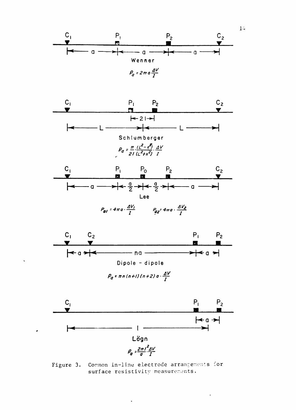
In addition to the Wenner configuration various arrangements of
current and potential electrodes can be deployed along the ground.
The Wenner set-up is commonly used in the United States, while the
Schlumberger configuration is more popular in Europe. Certain arrays
in some areas may permit better evaluations of the subsurface and as
a result many different electrode arrangements are used and described
in the literature. Some of the more common in-line arrays and the
corresponding apparent resistivity equations are illustrated in Fig
ure 3.
Expression for Two Horizontal Layers
A method to calculate potential fields in a layered medium by
the use of electric images was introduced by Lord Kelvin (Sir William
Thompson) in 1845 and later applied by Maxwell in 1891 to parallel
boundaries. Both Hummel (1929) and Lancaster-Jones (1930) applied
the optical analogy to electrical currents to solve the two-layer
boundary problem. The potential difference which can be measured with
the Wenner array is derived for clarity here.
From Figure 4 conditions are shown where a positive source and
a negative sink at a finite distance apart represent the two current
electrodes. A parallel plane surface is introduced at a distance
below the ground so that a layer with resistivity p is bounded by two
semi-infinite media p and p . The combined effect of the two bound
aries in terms of reflection coefficients, k, produce an infinite series
of images so that the potential at any point on the surface is given by
K
K
JS.
- K a >+-<-
L
Wenner
XL H-2M
Sch I um berger
L
a
14
C2
-H
A .
Lee
Pai =^^0 zjk>
-H
C,
KaH<- na Dipole - dipole
Pfj^nn(nH)(ni-2)a-Y
-H a H
Figure 3
Logn
'a - a I
Common in-iine electrode arrancerients lor surface resistivitv measurements.

15
= k' l • - k ' l
' I ' I i I I I
= k'l • - k ' I -T- 4h
T 2h
T
I 1 I I ' Medium 0 I
n I - I
I Medium I i ^ I I J_ ,
V7777Z^777777P7777;7P77777777Z!7777777777777777777777777777777777777777777777 2 h I I
I Medium 2 i I , • = k ' l • - k ' I - ^ 4h
« I I I I I I ' i I 9 I 2
I2 • = k^I • - k ^ I
I I I I
i
Figure 4. Positions of near images due to a source and sink.

16
V = 27T ^ I
n=^ n 2k I
r " n n=l r
where p = resistivity of top layer
I = electric current
r = spacing factor
k = P2 - Pj
P2 ^ ' l
The potential at M is
Ip V = —
1 27T a za /?7 (2h) / ( 2 a ) ^ + (2h)
+ k / a ^ + (4h)^ / ( 2 a ) ^ + (4h)
+
Ip , n=°° - 1 + 2 y k""
n=l 47Ta
/ L + (^^) 2nh.2 a
/A + ( ^ ) 2
From the symmetry of the figure, at point N
V = -V . 2 1
Therefore, the potential difference is
\ - \ = \ - ( - ^ > = ^ \
Ip AV =
277 a
n= 1 + 4 I k"
n=l / 1 + (2nh)2 ^ ^ ^ 2nhj2 a a
or
AV = ^ ( 1 + 4 F ) . 2iTa

17
Thus
\ -^2 27Ta = p^(l + 4F).
The quantity p (1 + 4F) is denoted by p which is a weighted average
of the resistivity that may exist in a region within which the current
flows.
Then the apparent resistivity, p , for a Wenner array can be 3.
expressed as
Pa = Pl n=c
1 + 4 I k" n=l /l + (23!l)2 /, + (2nh)2
a a
where a = equal electrode spacing
h = thickness of first layer.
Multi-Layer Developments
Various numerical methods to calculate apparent resistivities
for multi-layers have been developed since Hummel's expression. A
form equivalent to Hummel's formulae was given by Stefanesco and
Schlumberger (1930) as
Ip 1 1 V = 27^ • + 2 / e (X , k, h) J (A^) dX .
0
Both Hummel and Stefanesco gave explicit solutions for two and
three layers and indicated the extension to more layers. The nomen
clature used in this discussion will not include the air layer; there
fore, the number of layers refers to the actual number of subsurface
layers including the infinite substratum or half space.
Ehrenburg and Watson (1932) used the principle of the image theory
to develop expressions for a six-layer case. Slichter (1933) expanded

18
Stefanesco's determinants and showed results for six layers. Recur
rence formulae for a six-layer case was shown by Fathe (1963) in which
he used Horner's procedure in algebra to find the roots of a reciprocal
polynomial equation. Onodera (1960) started from Fathe's paper to
determine recurrence formulae for a maximum of seven layers. The
kernel function was used by Van Dam (1967) for expansion as a series
in ke so as to denote results for six layers.
Approximation and Direct Methods of Calculation for a Small Number of Layers
Since the use of the above methods require long and tedious cal
culation processes, various approximation methods can be used. These
approximations are more applicable if only one or two interfaces are
present.
When only one interface is involved a direct interpretation for
h and k can be made from the simultaneous equations in the form
where p = p for small distances, a . Tagg (1934) has constructed
master curves to solve the function F which is the infinite series
containing the above h and k terms.
If one or more layers are added to the above equations, curve
matching techniques then become advantageous in the interpretation
of sounding data.
Standard Curve Compilations
As an aid to the interpretation of field resistivity data, master
curves for different parallel-layer earth models have been published.
19
Compilations of 100 curves or less include work by Roman (1934),
Watson (1934), Wetzel and McMurray (1937), Fathe (1955) and Koefoed
(1955).
The most extensive catalogues containing master curves are by
Compagnie Generale de Geophysique (1955) and those by Mooney and
Wetzel (1956). Compagnie Generale de Geophysique published an album
of three-layer curves for the Schlumberger array. Mooney and Wetzel
directed a group in the preparation of tables and related curves for
two-, three-, and four-layer cases for the Wenner array.
Other model studies for curve compilations have included vertical
or dipping fault planes, vertical dikes, filled sinks and buried
spheres.
CHAPTER IV
A RESISTIVITY COMPUTATION METHOD FOR
LAYERED EARTH MODELS
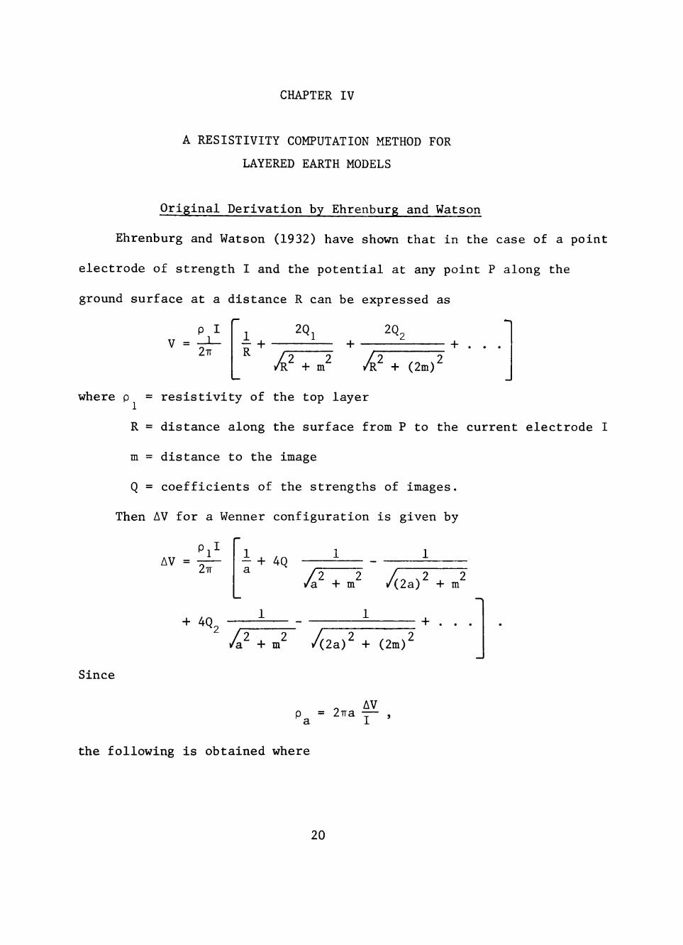
Original Derivation by Ehrenburg and Watson
Ehrenburg and Watson (1932) have shown that in the case of a point
electrode of strength I and the potential at any point P along the
ground surface at a distance R can be expressed as
V = P I 1
27T
2Qi 2Q,
R ri 2 •R + m
JFl (2m) where p = resistivity of the top layer
R = distance along the surface from P to the current electrode I
m = distance to the image
Q = coefficients of the strengths of images.
Then AV for a Wenner configuration is given by
AV = 2TT
+ 4Q / 2 . 2 •a + m /
+ 4Q,
(2a)^ + m^
+ . . . J^ + m /(2a) ^ + (2m)
Since
p = 27Ta — , a 1
the following i s obtained where
20

21
2.a Pl^ P = • ^a I 27T
+ 4Q
/ ^ + m^ /(2a) + m^
+ 4Q
J^ + m^ /(2a) + (2m)
+ .
= p ri + 4a(Q P + Q P ^ + . . .)J 1 1 ai ^2 a2 ••
n=oo p^ =p [1 + 4a j; Q P _ ] . a 1 n=l n an
where a = electrode spacing
m/2 = bed thickness.
Since P is a function of electrode spacing and bed thickness, an r o >
the main problem is to find the relationship of Q . Ehrenburg and
Watson used the optical analogy to build up a set of differential
equations to satisfy the necessary conditions. These differential
equations are then expressed as a set of algebraic equations to ob
tain the strengths of electrical image poles. Watson (1934) has given
formulae for layered media through Q in terms of reflection coef-
ficients.
Extension of Ehrenburg and Watson's Formulae
The equations for electrical image poles have been extended in
this thesis so as to include formulae sufficient for a maximum eleven-
layer sequence (Figure 5). The determination of the reflection com
binations became lengthy; therefore, a numbers search by computer as
described below was used to check these derivations.
Determination of Reflection Combinations
The number of combinations of selecting r objects from a set of
n objects is denoted by

Layer
Layer
Layer
Layer
Layer
Layer
Layer
Layer
Layer
Layer
Layer
0
1
2
3
4
5
6
7
8
9
10
^ 0
P^
Pz
Pz
^ 4
/>5
^ 6
Pi
PB
PB
P^o
ho
h,
he
h^
h4
h5
he
hr
he
h.
f^io
Layer I M P„ h„ L = Half Space
Layer I 2 j P^z h,2
-- 3
8
.0
Figure 5. Nomenclature for layers, earth model

23
C = P / r ! . n r n r
Then t h e number of combinat ions for n l a y e r s t aken s u c c e s s i v e l y
1 , 2 , 3 , . . . , n a t a t ime i s
C, + C_ + C_ + . . . + C = 2 ^ - 1. n l n 2 n 3 n n
A computer program was written to search for all permutations
for a maximum of ten layer boundaries with the necessary number of
nested DO loops. The combinations of the reflection interfaces were
printed out from corresponding IF statements so as not to permute the
reflections among themselves.
Formulae for Electric Image Poles
The original equations through Q are repeated below for conti-5
nuity. The expression for Q by Watson (1934) was found to be in error 6
and has been corrected in this study. Since these expressions for
shallow image poles become quite lengthy past Q , the remaining equations 7
are not given in their entirety in the text.
Q = A 1 1
Q = (1 - A ^)A + A Q 2 1 2 1 1
Q = ( 1 - A ^ ) ( 1 - A ^)A + (A - A A )Q + A Q 3 1 2 3 1 1 2 2 2 1
Q = (1-A ^ ) ( 1 - A ^ ) ( 1 - A ^)A + (A -A A -A A )Q k 1 2 3 k 1 1 2 2 3 3
+ (A -A A +A A A )Q + A Q 2 1 3 1 2 3 2 3 1
Q = (1-A ^ ) ( 1 - A ^ ) ( 1 - A ^ ) ( 1 - A ^)A + (A -A A -A A -A A )Q 5 1 2 3 k 5 1 1 2 2 3 3 4 4
+ (A -A A -A A +A A A +A A A -A A A A )Q + (A -A A 2 1 3 2 4 1 2 3 1 3 4 1 2 3 4 3 3 1 4
+A A A +A A A )Q + A Q 1 2 4 2 3 4 2 4 1
24
Q = (1-A ^)(1-A ^)(1-A ^)(1-A ^)(1-A ^)A + (A -A A -A A 6 1 2 3 4 5 6 1 1 2 2 3
-A A -A A )Q + (A -A A -A A -A A +A A A +A A A +A A A 3 4 4 5 5 2 13 2 4 3 5 1 2 3 1 3 4 1 4 5
-A A A A -A A A A -A A A A )Q + (A -A A -A A +A A A 1 2 3 4 1 2 4 5 2 3 4 5 4 3 1 4 2 5 1 2 4
+A A A +A A A +A A A -A A A A -A A A A +A A A A A )Q 2 3 4 1 3 5 2 4 5 1 2 3 5 1 3 4 5 1 2 3 4 5 3
+ (A -A A +A A A +A A A +A A A )Q + A Q 4 1 5 1 2 5 2 3 5 3 4 5 2 51
Q = (1-A ^)(1-A ^)(1-A ^)(1-A ^)(1-A ^)(1-A ^)A + (A -A A 7 1 2 3 4 5 6 7 1 1 2
-A A -A A -A A -A A )Q + (A -A A -A A -A A -A A +A A A 2 3 3 4 4 5 56 6 2 13 2 4 3 5 4 6 1 2 3
+ A A A + A A A + A A A - A A A A - A A A A - A A A A - A A A A 1 3 4 1 4 5 1 5 6 1 2 3 4 1 2 4 5 1 2 5 5 2 3 4 5
-A A A A -A A A A )Q + (A -A A -A A -A A +A A A +A A A 2 3 5 6 3 4 5 6 5 3 1 4 2 5 36 1 2 4 1 3 5
+ A A A + A A A + A A A + A A A - A A A A - A A A A - A A A A 1 4 6 2 3 4 2 4 5 2 5 6 1 2 3 5 1 2 4 6 1 3 4 5
- A A A A - A A A A - A A A A + A A A A A + A A A A A + A A A A A 1 3 5 6 2 3 4 6 2 4 5 6 1 2 3 4 5 1 2 3 5 6 1 3 4 5 6
-A A A A A A )Q + (A -A A -A A +A A A +A A A +A A A 1 2 3 4 5 6 4 4 1 5 2 6 1 2 5 1 3 6 2 3 5
+ A A A + A A A + A A A - A A A A - A A A A - A A A A 2 4 6 3 4 5 3 5 6 1 2 3 6 1 3 4 6 1 4 5 6
+A A A A A +A A A A A +A A A A A )Q + (A -A A +A A A 1 2 3 4 6 1 2 4 5 6 2 3 4 5 6 3 5 16 1 2 6
+A A A +A A A +A A A )Q + A Q 2 3 6 3 4 6 4 5 6 2 6 1
Q = (1-A ^ ) ( 1 - A ^ ) ( 1 - A ^ ) ( 1 - A ^ ) ( 1 - A ^ ) ( 1 - A ^ ) ( 1 - A ^)A 8 1 2 3 4 5 6 7 8
+ (A -A A -A A -A A -A A -A A )Q + . . . + A Q 1 1 2 2 3 4 5 5 6 6 7 7 7 1
Q = (1-A ^ ) ( 1 - A ^ ) ( 1 - A ^ ) ( 1 - A ^ ) ( 1 - A ^ ) ( 1 - A ^ ) ( 1 - A ^ ) ( 1 - A ^)A 9 1 2 3 4 5 6 7 8 9
+ (A -A A -A A -A A -A A -A A -A A )Q + . . . + A Q 1 1 2 2 3 4 5 5 6 6 7 7 8 8 8 1
Q = (1-A ^ ) ( 1 - A ^ ) ( 1 - A ^ ) ( 1 - A ^ ) ( 1 - A ^ ) ( 1 - A ^ ) ( 1 - A ^ ) ( 1 - A ^) 10 1 2 3 4 5 6 7 8
(1-A ^)A + (A -A A -A A -A A -A A -A A -A A -A A )Q 9 10 1 1 2 2 3 4 5 5 6 6 7 7 8 8 9 9
+ . . . + A Q 9 1

25
11 (1-A ) ( 1 - A 2 ) ( i . A 2 ) ( i _ A 2 ^ ^ ^ _ ^ 2 ^ ^ ^ _ ^ 2 ^ ^ ^ _ ^ 2 ^ ^ ^ _ ^ 2
2 ^ 2 "" ^ ^ ^ ^ (1-A ) ( 1 - A )A + (A -A A -A A -A A -A A -A A -A A -A A
^ 10 11 1 1 2 2 3 4 5 5 5 6 7 7 8 8 9 -A A )Q + . . . + A Q
9 10 10 10 1
From the above the following recursion formulas result for the
deep image poles.
n=oo
Q = (l-A^)A + I A Q ^ 1 2 ^ t o 1 n - 1 n=2
Q = (1-A 2 ) ( 1 - A 2)A ^ 1 2 3
n=°° n=<» + I (A -A A )Q + I A Q -
n=3 1 1 2 n - 1 ^ ^ 3 1 n - 2
Q^ = (1-A ^ ) ( 1 - A ^^ ' • ' - 2 n 1 2
n=<» ) ( 1 - A )A + y (A -A A -A A )Q ,
3 4 ^^^4 1 1 2 2 3 n - 1
n=oo n=oo
+ I (A -A A +A A A )Q . + J A Q ^=A 2 1 3 1 2 3 n - 2 ^f:, 3^n-n=4 n=4 3 n - 3
Q^ = (1-A 2) (1-A 2 ) ( i _ / 2 . , , . 2 n 1 2
n=oo
n=oo
A ) ( 1 - A )A + y (A -A A -A A -A A )Q , 3 ^ 5 j^=5 1 1 2 2 3 3 4 n - 1
+ I (A -A A +A A +A A A +A A A -A A A A )Q ^ n=5 2 1 3 2 4 1 2 3 1 3 4 1 2 3 4 n - 2
n=oo n=oo
+ y (A -A A +A A A +A A A )Q ^ + y A Q , n=5 3 1 4 1 2 4 2 3 4 n - 3 ^^^ i+^n-4

CHAPTER V
SURFACE RESISTIVITY PROGRAM
The principal task of this program is to compute apparent re
sistivities for parallel-layer earth models when the Wenner electrode
arrangement is used. The exactness of the computed apparent resistivity
values as determined from single precision arithmetic is limited only
by the accuracy of the computer used.
The shallow image pole strengths, coefficients Q(l) through Q(ll),
are sufficient for a layered model up to a maximum of eleven layers.
Each coefficient in the program includes all preceding coefficients
SO that 2 -2 reflection combinations are contained in each equation.
Since the coefficient formulae became rather lengthy, these arithmetic
expressions have been separated into individual statements so as not
to exceed 250 syntactical units.
These equations reduce to more simplified forms when any of the
reflection coefficients, Al through A9, are determined to be zero from
the true resistivities and layer thicknesses. When the required
number of coefficients are computed for a model, a transfer is made
to the proper recurrance formulae so as to generate the deeper image
poles internally. Iterations from DO loops eliminate the mul
tiplication by any reflection coefficients that may be zero as deter
mined from the shallow image poles.
The main input for individual models includes true formation
resistivities, thicknesses of individual layers and electrode spacings.
26

27
Input parameters are used to select the desired tables and graphs for
the output.
Convergence Properties
The coefficient patterns were examined for different layered models
Some representative Q(N) patterns for designated models S, T, U and V
are illustrated in Figures 6 through 9.
Since the calculations to determine the apparent resistivities
involved an infinite series resulting from Q(N) coefficients and the
distance equation P , it was necessary to terminate the summation an
process by some criteria. The proof of the convergency test is shown
below where
Therefore,
u = S - S . n n+1 n
lim u = lim (S , - S ). n n+1 n
n- ^ n^^
From this the series may be convergent if S and S approach the
same value and thus.
lim (S ,, - S ) = 0. n+1 n
n-x"
Then applying this test to the Q(N) illustrations, it is seen that
the series will eventually converge for model T; but does not converge
for models S, U and V. If some finite number, £, had been selected for
model V; in this case il = 59, then the following would have been ap
plicable
lim (S T - S ) = 0. n+1 n

'-^n s ....
• .(Ml C t»f ll. I ts'S •
-»•" -O.S 0.0
« c • • « « X
B S B « S S « B * * K B « S S a S
100*
Figure 6. Q(N) coefficient pattern for model S
28

29
• • * • . "Ol iCL I • • • « •
• oiNi coE^ricUNrs •
- I . O - 0 . » 0.0
ObO*
oao*
too*
Figure 7. Q(N) coefficient pattern for model T

. . . ..„, 3 0
• J.S
a • K
• • • «
100*
Figure 8. Q(N) coefficient pattern for model U

• CIS) COEFFICItMS •
-t.O -0.* 0.0 'O.^
Q*0-
ODD
100
Figure 9. Q(N) coefficient pattern for model V,

As n is allowed to increase to 64, it is seen that
lim (S , - S ) ? 0 ^, n+1 n
n=64
Now consider the series where
32
n=oo
an ^, n=l /l 2~2 / 2 ^ 2~T
/a - n m /4a + n m
If
lim T = T;
n-x» n
therefore,
lim — n-Kx) n
1 T
Then,
l i m C n-x»
S n
1 T
n = C (lim S )(lim — )
n 1 n-H» n- ^ n
where C = constant,
Since
lim — ^ 0; n-<» n
therefore.
Since it was found that
P ^ 0 as n ^ 00 an
-1 < Q(N) < 1,
the following is true
lim C n- <» n
= I
Consequently, p ^ L when applied to
Pa = Pi 1 + 4a[(lim Q )(lim P )] n ^ an

33
where £ is limited only by the available storage space for Q and
P . an
The desired accuracy for p can be determined if p = L for n a a
and n+1 by comparing apparent resistivity values. This is easily done
by terminating the series at a finite number, n, and then visually
comparing a specified number of computed p values. An alternate a
method is to use the function a - [a,/a la where [x] is the integer 1 1 2 2
whose magnitude does not exceed the magnitude of x and whose sign is
the same as the sign of x. When the modular arithmetic function
(a ,a ) is used to compare significant digits, the series can be ter
minated as a selected accuracy and compared to previously stored p ci
values to determine the convergency.
Subroutines
The two FORTRAN plotting subroutines were written for use with
a line printer and do not require special plotting equipment. A brief
discussion of both subroutines is included to describe the program
ming used to obtain these detailed plots.
Plot Subroutine No. 1
This subroutine plots the patterns of the Q(N) coefficients stored
in the main program. A Hollerith field in the main program is used
to print the graph heading across the paper for the designated x-axis.
Then a one-dimensional variable is set up on the subroutine so as to
contain 101 elements named BLANK. A positive integer is computed from
NDX = (PT(I)/.02) +51.5
where PT(I) = Q(N).

34
The side of the axis is determined by an IF statement that trans
fers to one of two DO loops J = 51, NDX or J = NDX, 51 that place a
designated symbol EPLOT in LINE(J). The variable LINE is printed from
an alphameric field lOlAl and the above process is repeated down the
page until N is completed. A numerical value from the DATA statement
is printed every 20th time at x = 0 to denote the number of coefficients
printed along the y-axis.
Plot Subroutine No. 2
This subroutine is used to plot apparent resistivity versus
electrode spacing on a 10 x 10 inch graph. A maximum of eight curves
in the form y = f(x) can be plotted using the symbols
A B C D E F G H .
Values to be plotted from the main program are stored in a one-
dimensional array designated by
ROEIl R0EI8
ROEAPl R0EAP8
where ROEIl . . . = true resistivity of the top layer
ROEAPl. . . = apparent resistivity for increasing electrode
distances.
The electrode distance is determined from the input data where
the spacing choices are 2.5, 5.0 and 10.0. After the values for the
designated number of curves per graph are computed in the main program,
the subroutine is automatically called.
The value of the resistivity of the first curve is determined
from
35
I = (ROEIl(l)/(SROE*0.25)) + 1.5
I = (ROEAPl(JR)/(SROE*0.25)) +1.5
where SROE = scale factor for horizontal axis
JR = identification of electrode spacing number for vertical
axis.
The multiplication by 0.25 determines the proper value for the
horizontal scale while the added 1.5 includes 0.5 for rounding purposes
and 1.0 to establish the zero plot value. The proper alphameric
character is substituted for the computed integer in the relationship
SYMBOL(I) = A. The above process is repeated until all alphameric char
acters are stored in the single-dimensional array containing a maximum
of 101 spaces. This array is then printed and the above process is
repeated until the proper number of electrode spacings is completed.
An intrinsic coordinate system is used to plot the grid patterns
and label the x and y scales for the selected graph scale. A lack of
resolution for a few curves may require the option to print the tab
ulation of electrode spacings versus apparent resistivities so that
more accurate values can be obtained.
The plots obtained were printed with a line printer set at a
vertical spacing of six lines per inch. Since the vertical spacing
and the type print spacing were not equal, a distortion of 0.9:1.0
is inherent. Examples of model parameters input, tabulations and the
resulting x-y plot are shown in Figures 10 through 13.

36
I / )
OJ
< or < o a.
Ul o o o O T. X
• »/> »A »/* */^ »/»
l/> . - ^ . - . - . -0( _ _ _ _ _ ui I T 7 r 2
• >- 3 3 3 3 3
• -< z z z: z z I I I X I
• U. o o c o c o
o o o o o i/» > o o o o o ^ t- o o o o o l i i < . H O o * ^ > o m o t / ^ o O "^ O o "« *-_ #•> O o *^ fc^ tL f^ O o "^ _ U. < « 0 « 0 0 0 0 - C 0 ' ^ 0 «rt UJ . • • • # . . * • • * OJ 0 0 0 0 0 0 0 0 0 0 3 0 X I I I I I U I I I I I I I
o 1 r O • • • l i l l l l l i l l i l t i l « _ 4/t t / l 1/1 v^ OJ ^ . « _ _ _ M _ _ _ . . _ _ . ^ . . ^ k - t j O _ r g # » N ^ t r - 0 ^ " C D ^ C — t/ _ _ _ _ < Ui _ _ i n Z ? 2 ' Z O . J _ _ _ _ _ _ _ _ _ _ _ lii 0 3 3 D I / 1
u/ at O C o C u. ec o • • • . -J
_ ir o i/> o « I . . cv r» (»< X
i/i */* ^ - • - -y/S ^ ^ ^ . ^ —
' O I O i O i O o
I o
O ' O ' o • O ' o O '
r z 3 3 z z X r
z z
c 5 • •
•r c
u. < n « 0 0 0 0 0 0 - 0 ' ~
UJ o o o o z z
o u z o
u Ui .J
o o o o o o o o o
o o o z
^ *A . r . - _
— — ^ z r z £ -< < < < < « < < < « « z — — -
a< C C C C . O t • • • _ _ IT iT ^ i - «
>
Ui at z 3 z
s z 3 z
cr.
o
< < a.
z
o o
o O ' o O * o o *** O O '* o o •" o o **
O O O O ' O O O O ' ^ O
• 3 0 0 0 0 0 0 0 0 0
I/I
Ui > •
4
^ u. o > •
.-« •
> . •
l/> */> i/> (/) Wl
^ ' .- .- ^ z z z z z 3 3 3 3 3
z z z z z Z X X Z X
o o c o o o o o o o o o o o o o o o o o • • • • • o IT o <r o _ XV _
I I I I I o
Ui O ? ? C O O i i a i i i i i i i i < O Z _ VI vn ^r X ^ — — — — . . - . - _
O - . ( M ^ ^ J ^ ^ ^ - C O ^ C - . i/t _ _ _ l U i _ — V » 2 Z Z . . J _ _ _ _ _ _ _ _ _ _ _ UJ 3 3 3 ec u. < < < « < < < < < < < z < u ac O C O UJ flf o * . t
_ «r o / X — c —
t/) Ui
— < ^ a.
o < •O T
1/1
Ui o 3 O O Z z
ec UJ ^ » ^ . . . « . SC » . ' ^ f.^ ^ ^ z 3 _ Z . J - i -J - I - I
y/\sA ^ ^ --t/> _ _ _ _ —
Ui -z z r r ^ • > 3 3 3 = r
4 • ^ Z Z X z z
r r X X X • u. c ;; c ; X
o o o o c r
vn > o o c c -. - . - O 3 C C C Z * * ^ O C '* •" . . • • • u i i ^ o o 1^ > o j " C i - r ^m fl\ o o ^ _ — - ^ - « VJ f* o o ^ . -_ ** o O '^ */ IL **> O O "^ "" u. " ^ O O - C O O - C O O - ' O .^ Ui . • • . . * * • • • • u. 3 O O O C O O O O O O O t I I I ' t O I I I I I • 1
o z z o * • • • < _ 1/1 */l ^^ . - _ o ^ r > i # A . i > i r < c ^ e o ^ o - " * _ - . _ — < oi . . _ * / ^ 7 : ' ^ * i . J _ _ _ _ _ _ _ _ _ _ _ u, X X 3 I : . " u. < < < < < « < < < < < Z u. X c c c : _ D C < _ > • • • • —
— f IT ^ .' < Z - " * •* -^ X
Ui — . - « • » » - . S — ">< ^ * . -z 3
3

37
i/> *rt <•> ^ i / i */» ^ - ^ ^ ^
v> ct UJ
^ Ui
z < K
< o CL u
-J UJ
MOOE
MOO
RTH
H-Z U i • -
u
.— U. U. Ui
o u
CTION
Ui
u.
1/s |. #^ lA in r- ^. irv m rg rg lA lA ^- ^. lA lA CM rsi t/> ir K ^. lA m O ^ j O O O O A i O J ^ • • » • • • . « • • O O O O O O O O O O
1 1
- . f s J r ' ^ ^ l / ^ ^ ^ . « f f ' 0
*
O
. o
_ • ^
¥' * •
> * M
^ (/) * r t
t/1 Ui
« ra z <
i n
Ui
z
Ui
> -1
u. o
>-• -
"-> •-
z z z z z 3 3 3 3 3 z z z r z I X X r r o c o o o o o o o o o o o o o o o o o o * • • • • O rf\ o m o
- . I.S rg j . \ - .
I I I I
I I I I
I iA Ui
ec « Z a.
Ui o o o o z z
in
VO 1/* t^ «/ i^ l/> _ . - t - •- ^ ac _ _ — Ui z z z z 2-> 3 3 X 3 : ^
- I Z Z T Z Z X I I I I
u. O o c o o o
o c o o o > o o o o o >- o c o c o
> O "J" O J" o — _ - ^ rg -»• _
u. i / v O O ' N i O O ' N O O k J ^ O »/>
O O O O O O O O O O O O I I
I I I I
z z z 3 3 3
z a. 3 </>
O o c o u. I o m o « I I.S ^. pn I
-« r« m •# m
ec «
o z z o • • • • • • « • • \/t ^ ^ ^ OJ N. * « « — * » * - ^ - * _ — * » - » • ^ _ ^ ^ i ^ o - . f N i » . * . t t r - c f * e o c " 0 — */» _ — _ _ ^ Ui — — v i i ^ z z z a . _i _ — _ _ UJ 3 3 3 3 v ^
». c c c o — J^ J-Z — .» •r X
UJ ^ — .» .« — A . * P f« ^ ^ z 3 Z -I -I -I -I ^
O
>% I X
U o
>-l
CO
1/1«/) 1/1 i/> • - . - • -ec _ _ _ Ui z z z >- 3 3 3
Ik
O
</) ec Ui
»• Ui
z < oc « Ui Oi
^ ^ UJ
MODE
MOO
z
ec < Ui
•
i / i
-z Ui
.« o
.« u. u. ut o o
CTION
Ui
a. UJ oc
• •
i»i
<n m f\ <n i»i
• o o o o o o o o . « • • • • • * o o o o o o o o
^oiP' i^ino^^oD
o • o
o-
m CN
!.> JO t*\
m * t
o 1
o -
o . o
_ m^
> •
»• .* > .. »-I/I * • Irt Oi
ec o z <
1/1 I/I Ui z >c
THIC
•
z z Z X o o o o o o o o
I « •
1 o o 1 M - .
I I I I
I/I Ui
_ < z o. 3 i/l
i i l OC
u. o
l/>
oc
z « ec < u. a
-I .J Ui Ui o o o o z z
o o
in »o #.1 in m h- K. m in j\j t\i it^ in f- ^- »n rf^ «N rg vn in h- »^ in i n i N i o o o o o o ^ i n o • • • • • • • • • • • O O O O O O O O O O O
I I
I/l */» I/l /l l/t
z z z z z 3 3 3 3 3 z z z z z X I X r I O O O D 3
O o o o o o o o o o o o o o o
t • • • •
o .n o m o
I I I I
> in < 1 Kl z
at UI — — —
3 Z ^ - I - I
OC
o z z o • • • « • • « MB l/l l/l 1/1 I/l UJ ^ ^ ^ ^ ^ ^ ^ ^ ^ ^ ^ ^ . » - _ » . M . O o _ r s ( ' ^ ^ l n c ^ - a o c - o - ^ IJ _ _ _ _ < Ui _ — i / I Z Z Z Z Q . J _ _ _ _ _ _ _ _ _ _ _ UJ X 3 3 3 I / 1 U. < « • « < < < < < < < « Z UJ X C C C C U. oc U t • • t _J
• • w ij^ rf^ »n < I _ _ o — r
ec Ui .» — ^ , . - . oc _ -Nj "^ * rfi z 3 Z ^ -J ^ ^ -I
o S
u <u
(U
3 W) •H

38
o * * • • • • • • • • • •
» C- <>i ^ ® ' ^ -^ ^ 9 '^
0 « * « * * ' • • • • • • # • • • • • • • • • • • • •
o « « * * * « * * « « < « » « • •
> [ • - — — ^ ^ ^ ^ ^ ^ — ^ - ^ — ^ ^ ^ • * ^ ^ , * — ^ ^ ^ ^ ^ ^ ^ w ^ — — — — — — — ^ — — - - ^ . - — — — — — — — ^ — — . - — — — — — — —
Q • • • • • • « . • • •
e P » * r - f C * ' ^ ' V
« <0 « 4 <£ ^ < £ < C ^ l ^ ' t / * l / ^ ^ t f ^ < ^ ^ ^ 't ^ •* ^t
— O • t • •
« X — ^ ^ — — ^ - - ^ — — — — - . — — — — — — — — — — - — — — — — — — — — - • — — — - — — ^ — — — — — — — — - -
lAJ
or
Z w O f ^ - f «*^<^ 'C»*-**^ '^ -« -C 'OXO^*f l03 ' f f^"* 0 ' * * * 0 ' O f f c C i O ' ^ f f ^ 9^ r^ ^ &• t^ ^ ^ ^^ w 9 9 9 9 <y ( ^ x « ' ^ ^ l ^ * rs, — ctr**- ^ -r ^^ u J u * o < ^ ^ r < ^ ' ^ « c ^ • < r i * • t f ^ * x C ' ^ ^ / ^ • * < ^ - • ' ^ ^ ^ ^ < ^ c — f ^ J ^ ^ r f ^ ^ ^ ^ x e o < ^ ( ^ t ^ o o o o o o c c c o o c c o o o c c o c ? < ^ ^ • 7 • ( y ( ^ © • • • • • • • • • • • • • • • • • • • • • • • • • • • • • • • • • • • • • * • • • • • • • • • * O o < ^ < ^ e o * » * • » * ^ • ^ * ' ^ ^ * ^ " • « ) « o f l o e c c ^ c ^ a ' ( ^ < ^ o o o o o o o o o o o o o o - ^ - - — — • - — - ^ - ^ - ^ — — - - — — — •— — — — - - 0 0 0 0 0 a . z - « ^ — — — — — — — — — — — — — - . - — - . - • - i — — -. — — — — — — — — — -• — - — - — — a 4
» O 'Ni r ^ - * lA o -^ (^ «D «r O -J o <M -« o a Z UJ O ^ *^ <D "*
-* c o o o (^ <^ oo oc « K —
(0 3 W M a> > (0 bO
c •H O to a, CO
0) '13 O U 4J O (U
i H 0)
U-l o (0
c o •H iJ to
. H 3
X I to H
• 4-1 o
f H D.
>^ 1 X U O
U-l
(0 0)
•H 4J •H >
•H • P CO
•H CO (U M
4->
c (U M to a p. to
P^I^O-C-^'C^'C' • c o 0 e o e D x c o a ) « c a ) x x ( D ( O c o t f ) x a > ( ^ c ^ 9 ( ^ < ^ ( ^ c ^ ( ^ < ^ ( ^ c ^ ( ^ ( ^ < r ( ^ < ^ c ^ ( ^ c ^ 9
CM o o flC « o •- o u ^ o Ui u. O
' o t —
I I
^ X Nt 4> c ^ ^ ^ j ^ ^ « ^ 4> iT ^ ^ fNj ^ X ^ 1^ ^ ^ tr %r nT -c ^
o — ^ — -* '^ — ? »- C '^ /^
O O f f ' f f ' t t X f ^ o ^ o ^ ^ o t r i r ' t r ^ o ^ ^ ^ O ' C ^ ^ ^ ' C ^ ^ ' C C ^ ' O - C ' C ' C - o * ^ - ^ - ' ^ ^ ^ * ' ^ ^ ^ ^ ^ - * * - ' * ' ^ ' ^ * * ' * ' ^ ' * ' * ^ * * ' * ' * * '
(U
3 00
•H •4

o o
o a > •
I
o • o
o in
o o
o o ro
o O O
Figure 13. Representative x-y plot by computer.

CHAPTER VI
SUMMARY OF LLANO ESTACADO GEOLOGY AND HYDROLOGY
Geology
Sellards, et. al. (1934) and Frye and Leonard (1957) have studied
the geologic history of the High Plains. A brief summary of the re
gional geology is given here.
During the Mesozoic era subaerial erosion of the Permian beds
resulted in fine-textured sediments being deposited mainly in a flood-
plain environment. These strata of the Triassic system are known locally
as "red bed" rocks by water-well drillers. Erosion removed any Jurassic
sediments that may have been deposited and a part of the underlying
Triassic. An arm of the sea then covered this region during Cretaceous
time. Sands, clays and limestones were deposited in littoral and
epineritic environments, but erosion removed all or considerable portions
of these Cretaceous rocks.
Most authors agree the Ogallala sediments of Pliocene age were
deposited by streams in various stages of alluvial plain building that
originated in the mountains located to the west and northwest during
the Cenozoic era. These Tertiary deposits consist of beds and lenses
of clay, silt and gravel with caliche as a secondary deposit. Evans
(1949) proposed the Ogallala be considered as a group and that it in
clude the Couch and Bridwell formations.
The greatest amount of local orogenic movement occurred during
pre-Permian time and major structural features are not dominant in the
post Permian rocks as determined from petroleum exploration work.
40

41
Hydrology
Erosion has left the Ogallala Group of the Llano Estacado isolated
hydrologically from the surrounding areas, except through the under
lying rocks (White, et. al., 1946). This group lies at or near the
surface and its thickness ranges from zero to more than 600 feet in
some places. The saturated thickness also varies considerably, but
is being depleted rapidly from widespread agricultural irrigation.
At some places where little or no water is obtained from the
Ogallala, the older rocks become important as a ground-water source.
Most of the rocks immediately under the Ogallala are far less permeable
or they contain highly mineralized water, so usually they are not
sources of water.

CHAPTER VII
DETERMINATION OF ELECTRICAL RESISTIVITIES
ON THE LLANO ESTACADO
Information from Electric Logs
The number of electric logs obtained from water wells on the
Llano Estacado was limited. Petroleum bore holes were usually cased
near the surface; therefore, the critical near-surface electrical
properties usually could not be obtained from this source. The ma
jority of available electric logs were obtained from ten water test
holes in the Lubbock area. These drilled holes were logged with normal
AM and lateral OA electrode arrangements as a part of an exploratory
program for the city of Lubbock in 1945.
Lack of fluid in uncased holes or log calibrations near the sur
face prevented a specific determination of any resistivity contrast
between the dry and saturated Ogallala. Only a questionable contrast
could be observed from a few of the available electric logs. Below
the water table the Ogallala displayed a wide range of resistivities,
both vertically and horizontally. Numerous thin stringers of sands
and shales within the Ogallala made it difficult to predict the re
gional resistivities within this group.
The Cretaceous section, where present, displayed variable re
sistivities that indicated changes in lithology, porosity and perme
ability. The limestones within the section generally had resistivities
of 100 ohm-m or more.
42

43
The most conspicuous property observed from the electric logs
was the low resistivity of the Triassic when compared to the overlying
section. The resistivity range of this section was very low with
small lateral variations over long distances.
In addition to the electric logs, available spontaneous-potential
and radioactive logs were used as an aid to evaluate some of the for
mation changes.
Information from Surface Resistivity Measurements
In order to supplement the electric log data, numerous surface
resistivity measurements were made over the Llano Estacado. With a
portable resistivity apparatus electrical resistivities were determined
by deploying an expanding electrode separation over short distances.
This expanding electrode separation was necessary to insure that a
resistivity determination was not made of a thin weathered zone.
Surface resistivity determinations were made on outcrops of the
Bridwell and Couch formations of the Ogallala Group, the Comanche
series of the Cretaceous system, and the Dockum Group of the Triassic
system. The regional study of electrical resistivities also included
sand dunes, different playa lake sediments, caliche deposits and sat
urated sediments at various springs. A wide range of resistivities
was found to exist not only due to differences in lithology, but also
due to changes in water content and quality. These average regional
differences varied from 1.5 to over 100 ohm-m. In a few places dry
sands and caliche deposits near the surface indicated the resistivities
to be more than 500 ohm-m.

CHAPTER VIII
PARAMETERS FOR MASTER CURVE COMPILATIONS
The catalogue of master curves represents subsurface models of
the Llano Estacado determined from the regional geology, ground
water conditions and related electrical resistivity study. Simple
two-layer cases with various layer depths and resistivities were used
initially to represent the Ogallala and underlying Triassic.
Three-layer cases were then modeled with various thicknesses and
resistivities to represent two divisions within the Ogallala. This
extra layer represents geological differences between the upper and
lower Ogallala, or hydrological differences between a dry and saturated
zone when an overall electrical resistivity contrast is present in
the Ogallala Group. Variations of these models were also made in which
thin layers were added to delineate a soil zone, facies changes and
saturation differences. For some models a layer was added directly
over the infinite substratum to represent the Cretaceous above the
Triassic. Only simple models of the Llano Estacado were considered
in order to keep the catalogue at a reasonable size.
The concept of a parallel-layer case can be used on the Llano
Estacado, in most cases, because of the low rate of dip at shallow
depths. Aldredge (1937) has shown for dips less than 9 degrees there
is only a slight change in apparent resistivities when compared to
a two-layer horizontal case. The material within any given horizon
tal layer was assumed to be homogeneous and isotropic. An infinite
44

45
layer thickness of constant resistivity is applicable to the Triassic
as there is a lack of resistivity contrast within this thick section.

CHAPTER IX
CATALOGUE OF APPARENT RESISTIVITY CURVES
Description
The appendix contains 462 apparent resistivity curves for the
Wenner electrode set-up plotted in linear coordinate form. This cat
alogue was used as a basis for preliminary interpretations in the de
tailed area study. Although the catalogue was designed primarily for
the Llano Estacado; it is adaptable to other regions with small re
sistivity contrasts.
The reflection coefficient is a dimensionless quality so arbitrary
units (feet, meters, etc.) can be used for the models and associated
curve coordinates. Changes in depth proportions, apparent resistivity
scale and units of length can be used to obtain considerable varia
tions from this set of curves.
Accuracy
After the mathematical derivations and formula translation to
the computer program had been checked, several tests were used to
verify the results obtained from the coefficients and associated re
cursion formulae. These tests included (1) equating from longer to
shorter coefficient formulae for comparisons within the computer pro
gram and (2) comparing the computed values with published curves.
The comparison of published curves did not agree in all cases which
was attributed to approximation methods used by various workers. Mooney
and Wetzel used a reliability index for their curves and tables.
46

47
Most of the apparent resistivity calculations for this study were
made with the IBM 360 computer where the accuracy was to seven sig
nificant digits.

CHAPTER X
APPARENT RESISTIVITY CURVES FOR THE WENNER ARRAY
The eight basic types of apparent resistivity curves that were
computed for various layered models are illustrated in Figures 14
through 17. Curves that result from perfectly conducting or perfectly
insulating layers were not computed as the resistivity contrasts in
the region were too small to make this theoretical assumption. The
nomenclature for the various kinds of curves are the same as used by
Zohdy (1965a) to review four types of three-layer sounding curves for
the Schlumberger array. These type curves are designated minimum,
maximum, double-descending and double-ascending.
When sounding curves are obtained in the field, some preliminary
information about the properties of the subsurface can be obtained be
fore the complete interpretation is carried out. For example, when
the electrode separation, a, is small compared to the top layer thick
ness, then p = p. As the electrode spacing is increased, a greater pro-a.
portion of the current flows through the lower layer so eventually the
value of p asymptotically approaches the value of the infinite sub-
stratum, p . n
If two layers are considered with a constant first layer thickness,
h, only two possibilities exist between p and p when p ^ p . These 1 2 1 2
are p > p and p < p . The type curves that result are designated 1 2 1 2
descending or ascending as illustrated in Figure 14. This rate of
descent of ascent will be dependent on the reflection coefficient, k ,
48

49
• - ^ •
_^-« c_ •
^ a»-a: 3r-A^a'
ttr-^ a« «•-•. - r OJ X. a.~ 3. OJ ;L &. <L. a."'
Figure 14. Descending (A) and ascending (B) curves

50
F i g u r e 1 5 . Ilinimum (A) and r.axiraum (B) curves

51
*A^
3. 4. .fa.-*
^ a.-A^«? X c
Figure 16. Double-descending (A) and double-ascending (B) curves

Figure 17. Descending double-ascending (A) and ascending double-descending (B) curves.
53
and the depth to interface, h. As p ^ p for a constant p and h, 1 2 2
the point of inflection increases with the electrode spacing. When
k = 0 , then p = p and a straight line plot for apparent resistivity
versus distance will exist for an infinite homogeneous medium. For a constant p and p the rate of ascent or descent increases with an
1 2
increase in h. Since the resistivity contrast is dependent on the
factor (p -p)/(p + p ) , "mirror image" curves will not result when 2 1 2 1
the absolute values of the contrasts are equal.
When another layer of resistivity, p , is added; then four pos-3
sibilities exist among p , p and p . These are p > p < p , 1 2 3 1 2 3
p < p > p , p < p < p and p > p > p . 1 2 3 1 2 3 1 2 3
If p > p < p and p < p > p where h < h for a sufficiently 1 2 3 1 2 3 1 2
large h , two types of curves are possible when sufficient resistivity 2
contrasts exist. These are minimum and maximum types of curves as
illustrated in Figure 15. When the effect of p is suppressed as the 2
h :h ratio is decreased, the curves will become ascending or descending 2 1 types more dependent on p < p or p > p
1 3 1 3 When p < p < p o r p > p > p where h < h for a s u f f i c i e n t l y
1 2 3 1 2 3 1 2
large h , then double-ascending or double-descending curves are pos-2
s i b l e as shown in Figure 16. Due to the q u a l i t i e s of p < p < p 1 2 3
and p > p > p , the effect of the middle layer is usually hidden 1 2 3
and its influence is on the slope of the ascending or descending
curves.
The curves illustrated in Figure 17 were obtained as the com
plexity of the subsurface layering was increased. These curves are
designated as descending double-ascending and ascending double-de-

54
scending in this thesis. The lack of resolving power for the Wenner
array as discussed by Depperman (1956) and Unz (1963) did not pre
clude these types of curves. Similar types for the Schlumberger array
have been obtained by Fathe (1963) for a five-layer case in which the
infinite layer was considered to be a perfect insulator.
Other types of apparent resistivity curves were not obtained in
this study; instead, the curves degraded to the types discussed pre
viously. This was the result of one or more of the following:
(1) constant rates of increase or decrease in the resistivities of
the layers, (2) ratio of a bed thickness to its depth of burial and
(3) suppression of layers from the effects of the surrounding layers.

CHAPTER XI
APPLIED SURVEY IN THE YELLOW HOUSE CANYON AREA
Geography
The detailed electrical resistivity survey covered an area of
150 square miles in northwest Hockley and southwest Lamb Counties.
This area is designated the Yellow House Canyon area in this thesis.
In the central portion an undulating plain covered by native
grasses comprises 50 per cent of the area. The most prominent fea
tures in this part are the three large alkali lakes which are named
Bull, Illusion and Yellow Lakes. Only Bull Lake contained consider
able amounts of water during the survey.
The remainder of the land, more characteristic of the Llano
Estacado, has a level topography that slopes to the south-southeast
approximately 10 feet to the mile. This more level surface is used
for farming, both irrigated and dry-land. Prominent features in the
farming region are the numerous small dish-shaped lakes that contain
water only when an above normal amount of rainfall occurs.
Field Survey
The survey was carried out with a portable R-50 model stratameter
manufactured by Soiltest, Inc. of Evanston, Illinois. With the Wenner
configuration a direct current was applied to the earth through the
two outer electrodes and the resulting potential difference was meas
ured between the inner electrodes.
55

56
Stations were usually spaced at 1 mile intervals, but in some
instances the stations were as much as 2 miles apart due to inacces
sibility. Measurements were taken at 121 stations with an expanding
electrode separation ranging from 1 foot to 500 feet. From 5 to 20
readings were taken at each station.
Measurement Procedures
Resistivity measurements in deeply plowed fields and drainage
ditches, near cultural features or topographic irregularities were
avoided to minimize their effects on the readings. When possible
the electrode line was orientated E-W, otherwise the line was in a
N-S direction.
Before each measurement the potential difference caused by stray
D.C. potential was compensated. In some cases a weak secondary field
in the form of either a drifting or decaying action was present that
could not be nulled. Sometimes these natural potentials could be
minimized by replanting the electrodes or moving to another location.
If these secondary effects could not be eliminated from the main field,
then either an average determination was made or a first reading was
used. This depended on whether a pulsating or decaying effect was
present. The nature of this noise was not determined but could be
attributed to various sources such as telluric currents, stray power
line currents, electrochemical effects, induced polarization, etc.
At the short electrode spacings, care was taken so as not to drive
the electrode probes deeply in the ground. The theoretical assumption
of a point source is critical at very short distances.

57
During the survey differences in ground moisture from local rain
fall also affected the readings at very short spacings. To compensate
for these near-surface moisture changes so that the readings were rel
ative to each other, corrections were made back to a series of estab
lished base stations.
Reading Accuracy
The apparent resistivity for most electrode arrangements is given
by
. AV Pa = "l-
The majority of the resistivity measurements were made using a
constant current of 100 millamperes as recommended by the manufacturer
of the resistivity apparatus. When this constant current and a po
tential accuracy of ±0.0005 volt was assumed under stead state con
ditions, a limit existed in the reading accuracy of the resistivity
apparatus used. An effective 0.001 volt reading could be made if
p > 2.5 ohm-m at a - 140 feet. With the available cable lengths, a a —
0.001 volt reading was possible when p > 9.0 ohm-m at a - 500 feet. Si
If the potential was too small to be read at a given electrode inter
val, then it was necessary to increase the applied current.
For the outcrop measurements a technique was used in which the
apparent resistivity, p , could be read directly in the field. Within
a prescribed AV/I range the linearity of the resistivity apparatus
was established. From this the apparent resistivity can be read di
rectly if k = I; therefore, AV = p . Since k is a factor having units
of length, a conversion was applied so that the resulting apparent
58
2 resistivity determination was in ohm m /m (ohm-m) when the distances
were measured in feet.
Determination of Lateral Variations
Irregularities or "jumps" from some of the Wenner soundings in
dicated the presence of lateral resistivity variations in the area.
Carpenter (1955) described the use of the tripotential system with
the usual linear array to detect these lateral variations. If the
reciprocity theorem is applicable, then these lateral changes can be
detected as indicated by some of the experimental tripotential
soundings.
Geology and Ground Water
Triassic System
The Dockum Group of Late Triassic age occurs beneath the entire
area with an average thickness of 1500 feet. In the vicinity of the
three large lakes, where much of the overlying material has been re
moved, the Dockum Group is encountered at depths less than 50 feet
(Leggat, 1957). These beds are considerably deeper in other parts of
the area as indicated by the irrigation wells. Available water in
the Triassic is highly mineralized as determined from petroleum test
holes.
Cretaceous System
Rocks of the Comanche series of Early Cretaceous rest on the
eroded surface of the Triassic and are exposed along the western mar
gins of Bull, Illusion and Yellow Lakes (Grice, et. al., 1956 and New-

59
man, 1962). Erosion has removed much of the Cretaceous material so
that the aggregate thickness varies from less than 10 feet to more
than 200 feet. Small quantities of highly mineralized water are ob
tained from these rocks in some places.
Tertiary System
The Ogallala Group of the Pliocene series underlies all of the
area except in the vicinity of the alkali lakes (Cronin and Myers,
1964). To the south the thickness is less than 100 feet, while to
the north it has a thickness of more than 200 feet.
Some irrigation wells are located in the northern part of the
area, but the majority of the irrigation is concentrated to the south.
Water wells for domestic and livestock purposes are scattered through
out the area. Usually the water is very hard and in some places it is
too mineralized for use. The saturated thickness of the zone averages
from less than 25 feet to the south to more than 100 feet to the north.
Water-table depths decrease toward the alkali lakes where the water is
near the surface. The Ogallala yields very little water in many places,
especially in the eastern and western parts of the area.
Quaternary System
Thin deposits of Pleistocene and Recent age mantle most of the
area. The soils were probably developed and reworked during the mid-
Pleistocene epoch (Lotspiech and Coover, 1962). These deposits are
important hydrologically where they form catchment areas for rainfall
or for recharge facilities.

60
Interpretation
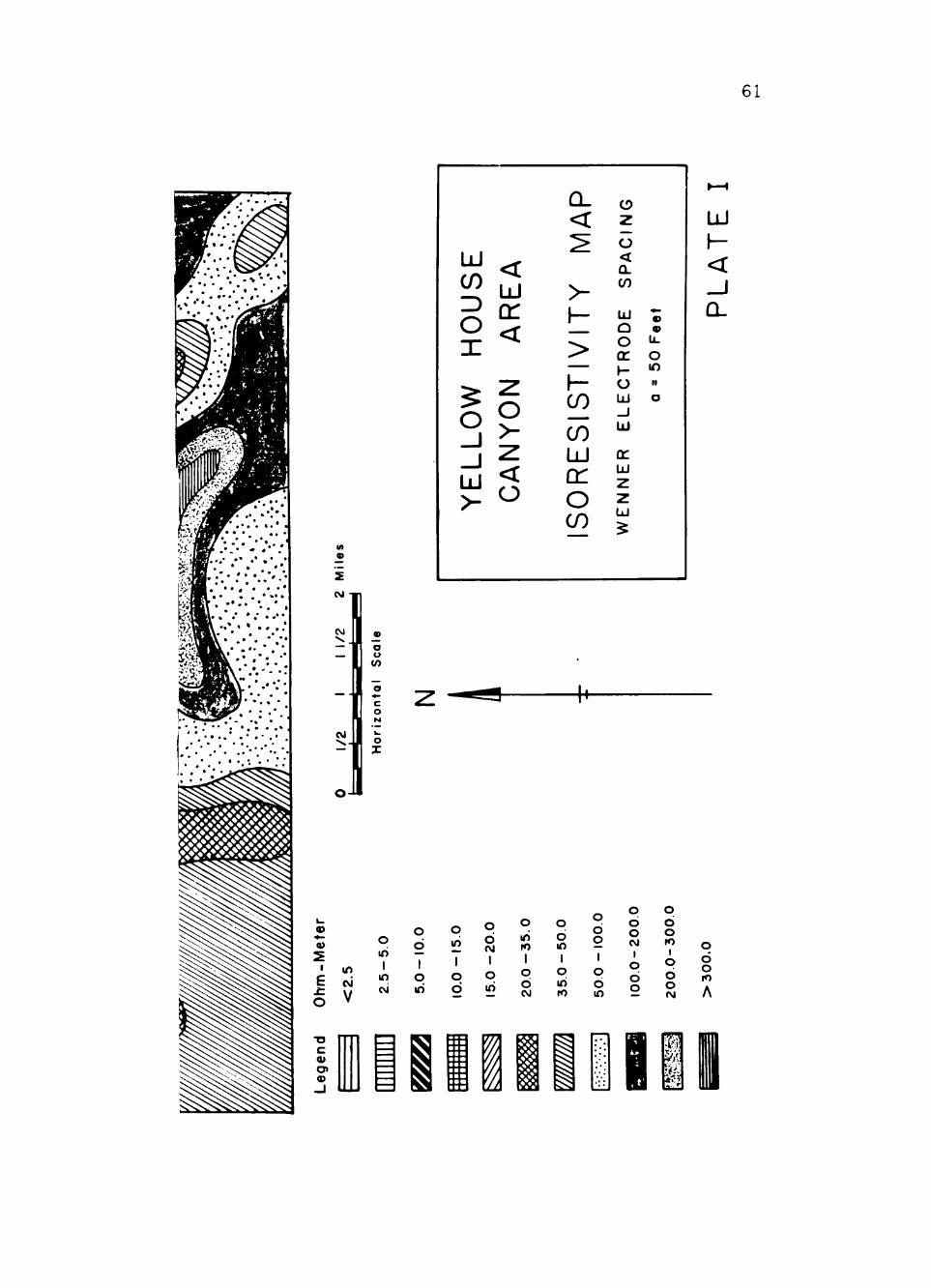
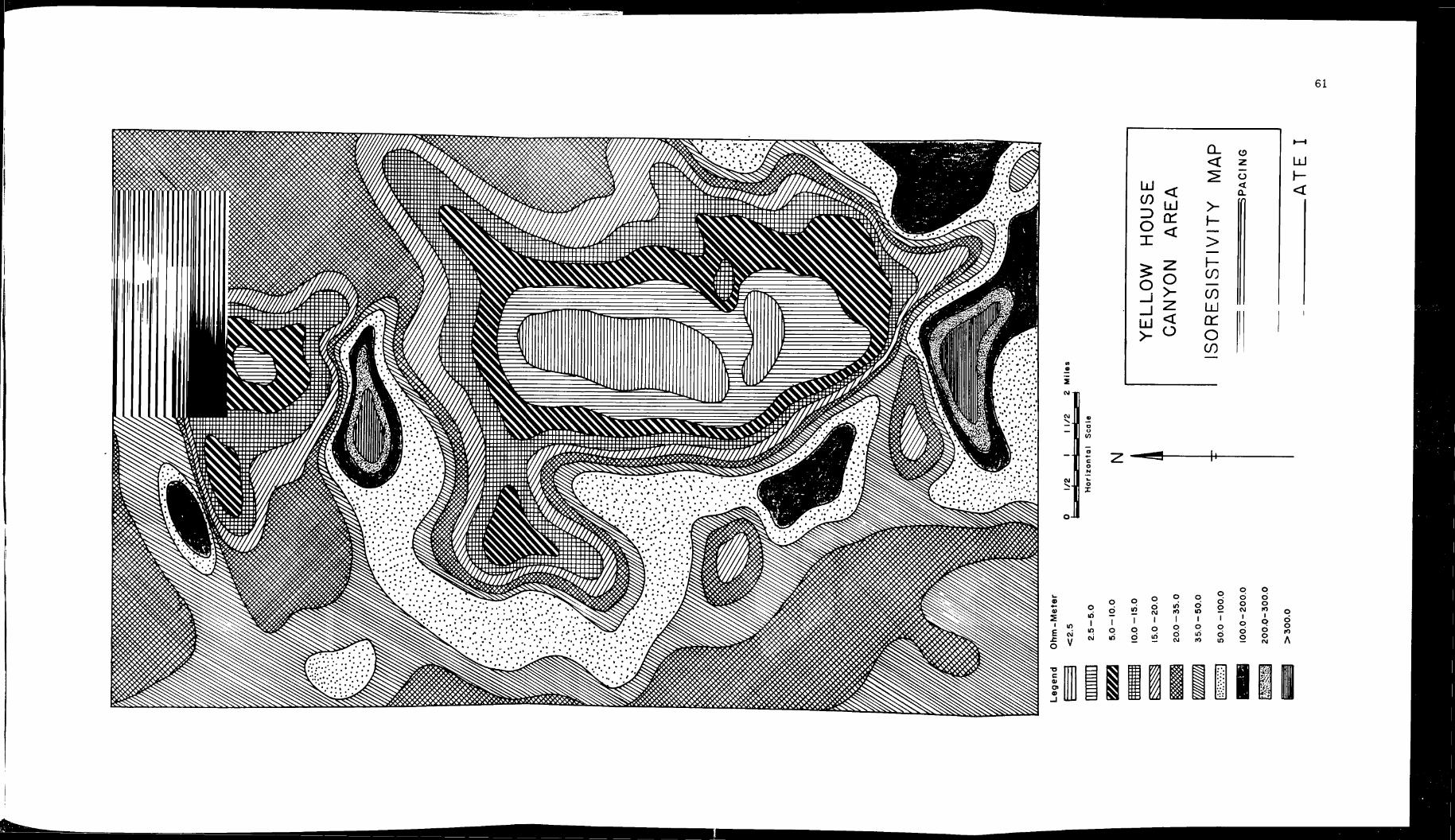
Isoresistivity Map
A contour map of equal apparent resistivities in the Yellow House
Canyon area (Plate I) shows the areal variations at a = 50 feet. This
electrode interval was selected as the most significant when the over
all changes in apparent resistivities were considered. Values obtained
from expanding electrode separations are evaluated in the interpreta
tion of the constant 50-foot electrode intervals.
The Triassic in this area dips to the southeast at about 13 feet
per mile as indicated from a few wells. Most of the interpretation
was made without subsurface control as data from numerous water wells
and seismic test holes were not available.
The most distinctive features of the map are the two large areas
of low apparent resistivities and a number of small anomalies dis
playing high apparent resistivities. The two large areas of low re
sistivities correspond to the three large alkali lakes and their
surrounding areas.
A considerable area around Bull Lake gives apparent resistivities
from 5 to 20 ohm-m. These resistivities result from the near-surface
Cretaceous deposits. Brand (1953) has mapped over 100 feet of Cre
taceous section in outcrops west of Bull Lake. When compared to some
of the regional Cretaceous determinations, the Bull Lake resistivity
values are somewhat lower. These lower Cretaceous resistivities are
probably due to the heterogeneous rock mixture. Brand (1953) has
measured considerable amounts of shale in the outcrop areas.
61
r • • • • . % • • • • • • • • • ^
-C . v - /
f .T"
. . . . cvi
CM
UJ CO 3 o X
o _ l llJ >
<
LU
<
YO
N
z. < o
Q_ <
^
>
h-
> •^^
S S
T
LU cr o
o z o < a. CO
UJ o o oc y-
EL
EC
oc UJ
z
WE
N
• u. o lO 11
o
o u
CM o X
4^
«
Q>
I
E
O
• o c a> o> a>
m cvi V
o in
I in
d 1 o m
in 1 o o
o 1 o in
o m
1
20
.0-
o o in
1
35
.0-
o d o I o d m —
o d o CiJ
I
o d o
o d o I o d o (M
UJ I -<
a.
o o lO
1
61
^S ?< X
'i IJ 5 ^ f^. > ^
CL (0 < 2 ^ o
< a.
>- fl h->
S S
T
LJJ Q: o
LU I -
- T X
ii M
^ z: c^
ii i :*s

62
A low resistivity anomaly was obtained on the plain located to
the northeast of Bull Lake. These low resistivity values here indi
cate the shallow sediments may contain highly mineralized water or
the Triassic is very near the surface. Regional dip does not indi
cate the Triassic to be shallow here. To the southwest in an area of
lower elevations, test holes indicate the Triassic lies from 5 to 10
feet below the surface of Bull Lake (Leggat, 1957). Lack of accessi
bility prevented the confirmation of these shallow depths.
The apparent resistivities rapidly increase away from the Bull
Lake area. This indicates the Cretaceous becomes deeper and/or thin
ner and the overlying sediments are increasing the apparent resist
ivities at these short electrode spacings.
Low resistivities of less than 2.5 ohm-m around the edges of
Illusion and Yellow Lakes were obtained. The low resistivities at
this shorter electrode interval indicate highly mineralized water in
the near-surface sands. The assumption of water-bearing sands below
the surface is based on the nearness of the soundings to the alkali
lakes. Changes in depth to the Triassic could not be established here
because of the inadequate resistivity contrasts. Regional dip indi
cates the Triassic is approximately 25 feet below the lake bottoms
of Illusion and Yellow Lakes. The sounding data indicated the Cre
taceous series is thin or contains water of high mineral content if
significant amounts of Cretaceous strata are present. Scattered sub
surface control shows the Cretaceous is thin under Illusion and Yellow
Lakes.

63
The gradual increase in apparent resistivities (2.5-10.0 ohm-m)
around the perimeters of the lakes indicate one or any of the fol
lowing: (1) decrease in the mineral content of the water, (2) de
crease in the saturation thickness, (3) increase in porosity, (4) in
crease in the Cretaceous thickness or (5) increase in the Triassic
depth. Constant or small resistivity changes were assumed for the
Triassic within this part of the area. Some of the descending curves,
when compared to the data near Illusion and Yellow Lakes, indicate
there is a high resistivity stringer above the Triassic. The re
sistivity contrasts and depth to thickness ratios were not sufficient
to produce any double-descending curves here. Sounding data farther
to the west of the lakes indicate the Triassic depth increases con
siderably.
A slight widening of the 5-10 ohm-m contour interval to the east
shows the influence of the sand-dune deposits along the eastern edge
of Illusion and Yellow Lakes. In this part of the area a 10-15 ohm-m
value is located on a topographic high of sandy material which indi
cates the influence of a dry-porous material near the surface and not
a Cretaceous remnant at depth. This was demonstrated by the sounding
data in this vicinity.
The anomaly of high resistivity that separates Bull and Illusion
Lakes indicates considerable deposits of different petrographic char
acteristics near the surface as shown by the quarry operations located
in this part of the area. A high resistivity anomaly does not sepa
rata Illusion and Yellow Lakes which indicates the sediments separating
these two lakes are similar to the lake deposits.

64
A number of small anomalies with high resistivities begin at the
north-central portion of the map and occur along the western edge of
the lake regions and then trend to the southeast. The topography along
this trend indicates these high resistivity anomalies are the result
of caprock deposits of indurated caliche. Numerous shallow gravel
deposits located in the area will also give these high apparent re
sistivities .
The low apparent resistivity areas to the northwest and north
east of the Illusion and Yellow Lake basin area corresponds to drain
age systems into Illusion Lake. To the southeast, low resistivity
values indicate a drainage valley out of the Yellow Lake basin. Con
siderable high resistivity material was measured on both sides of
this southeastern drainage system.
The resistivities become higher and more general further from
the lake areas which indicate small changes in the arid near-surface
zone. Any resistivity contrasts due to the presence or absence of
the Cretaceous and changes in the Triassic had little effect on the
apparent resistivity values at these short intervals.
Resistivity Profiles - Line A-A'
The E-W resistivity profiles at stations A-1 through A-10 (Plate
II) illustrate the differences obtained with an expanding electrode
separation (a = 5, 50, 150, 300 and 500 feet). These profiles show
a considerable transition as the line crosses the southern part of
the Yellow Lake basin. Only a qualitative interpretation is made at
the different electrode spacings. Existing information did not permit

in CD
I
1»»J U0|1D»»|3
o in Q lO O t^ in ei
JS|8n-u'M0 — ^(!A!ts|s*U tusJDddtf
UJ
o cr < CL I
< >-^- UJ
lO o o o o lO lO o o
— ro lo O O O D a
UJ I -< _J a.
CO
c/) UJ
i

66
a more precise interpretation. There would have been too many arbi
trary values involved to quantitatively interpret the sounding data.
The 5-foot electrode spacings showed considerable variations in
the conductivity of the soil. These apparent resistivities varied from
25 ohm-m at A-7 to 168 ohm-m at A-4. From A-5 through A-IO there
appears to be a shallow zone of variable materials as indicated by the
apparent resistivities at these shorter spacings. The low readings
at A-6 and A-7 are influenced by the Portales loam and Spur soils
that are common in the lake areas and small drainageways of the county.
Also, there is the probability the moisture content lowered the ap
parent resistivity at A-7. To the east at A-9, a small amount of
superficial covering may be present as indicated by the high resist
ivity of 106 ohm-m at the 5-foot electrode spacing. At the 50-foot
intervals the current penetration becomes deeper and a more combined
effect of the soil zone and the underlying less resistant material
is shown at A-5 through A-10.
To the west at A-4, a considerable amount of high resistivity
material is present near the surface which is indicated by high ap
parent resistivities at both the 5- and 50-foot intervals. The ef
fect with depth is also displayed at the 150-foot interval. These
higher apparent resistivities are caused by the indurated caliche de
posits that are exposed at this location. This phenomenon of a thick
cover with a constant resistivity exists 2 miles to the west, although
the resistivities are much lower.
The differences in apparent resistivity values at the 50- and
150-foot spacings indicate there are considerable variations near the

67
surface. These set-ups were all orientated E-W so the possibility
of the electrode line not being along strike was considered. Steep
interfaces from buried channel deposits in the Ogallala or erosional
surfaces of the Cretaceous would effect the parallel bed assumption,
if these contacts were of sufficient resistivity contrast combined
with a favorable thickness to depth of burial ratio. Azimuthal changes
of the soundings did not show significant changes in the apparent re
sistivities. The possibility of faulting was considered, but the more
detailed field plots did not indicate any fault-pattern curves.
At the 150-foot electrode spacings two average values exist along
the line. The higher values of approximately 35 ohm-m are present
from A-1 through A-5. To the east where the elevations are consid
erably lower, the values at this distance average about 8 ohm-m. The
only definite interpretation that can be made from the data is that
the Triassic is considerably deeper to the west.
Extensions of the electrode spacings were later made to 300 and
500 feet at stations A-1, A-4, A-7 and A-10. From these more com
plete data a double-descending curve was obtained at A-1 while the
other three stations displayed descending curves. Although stations
A-4, A-7 and A-10 show the same type curves, there were considerable
differences in their slopes.
The profile at A-7 indicates the Triassic to be approximately
100 feet. A value of 4.7 ohm-m at 500 feet shows very little, if
any, high resistivity material immediately above the Triassic. In
dications are the same conditions occur at A-10 with the higher re
sistivities at the 300- and 500-foot distances caused by a thick layer

68
of high resistivity material near the surface. West of A-7 the depth
increases considerably to A-1 where the depth to the Triassic was
determined to be approximately 250 feet.
Sounding Curves - Line B-B'
Sounding curves (Plate III) and associated electric log models
computed from the field data are illustrated for Line B-B'. This N-S
line was somewhat easier to interpret when compared to line A-A'. The
sounding data at stations B-1 through B-6 were of the same general
curve type, in which the apparent resistivity decreases with distance.
The asymptotic portions of soundings B-1 through B-6 indicate a
layer with a low resistivity and considerable thickness. Since the
water table at or near these locations was known to be at shallow
depths ranging from 6 to 44 feet; there appeared to be very little
indication of an electrical contrast between the low resistivity
Triassic and the immediately overlying layers.
Because the asymptotic values appeared to be rather low, it was
necessary to consider if the values were valid along this line. There
fore, it was important to (1) obtain some knowledge of the resistivity
of the Ogallala, (2) consider the presence or absence of the Cretaceous
and (3) evaluate the resistivity of the Triassic.
As discussed previously, the resistivity of a saturated formation
involves at least three independent variables. These are porosity,
degree of saturation and conductivity of contained fluids.
An estimate of the water resistivity was based on the conduc
tivity of water samples from Lamb County. In the Bull Lake area water
samples from nine wells used for domestic or livestock water gave a

69
NFIELD SOUNDING CURVES WITH
COMPUTED MODELS
• LINE B ^ '
PLATE in

%
h
ca
laU-BNIOVdi 3000133-13
I I I
\ I I'lj I t 1 ' ^ -*
h
03
!.k «
• ^ i -I I I
\
h
8-
njt-; v»=.
i
rr—t—r^- -t-
Ut
(0 UJ > a: 3 O
o Z I 5 t z i
SO
U 1
I ^ 1 u.
(f) _ ] UJ o O 2
o UJ 1— 5 a. 2" O o
.
_ -T. (D
UI
LIN
B UJ h-< _ ] Q,
$
X33d-N0llVA3-ia
I
IL^
H
I
s
8-1»
a I 9 8
1' l_
^ _ _ .
=^'
•9

'actor" was not
ition; i.e.,
basis of ir-
1 formation
with 10 per
entirely too
)unding curves.
and F values. t
iconsidered by
iase in the
Lty of the
jasonably per -
/ i t y of 20 ohm-m
with the data
J adjust the
cal l lake areas
v^^ /ing a whi te -
1 ind ica ted the
r e s i s t i v i t y
zent, an aquifer

70
specific conductance ranging from 665 to 8,030 micromhos at 25*0
(Leggat, 1957). Wilcox (1948) indicates a specific conductance of
2,000 micromhos (resistivity = 5 ohm-m) is a permissible limit for
water to be used for irrigation in Lamb County.
For a preliminary consideration the "cementation factor" was not
used in the evaluation of porosity and degree of cementation; i.e.,
m = 1. A 10 per cent porosity was first assumed on the basis of ir
rigation wells with small yields in the area. A 5 ohm-m formation
water resistivity in a 100 per cent saturated formation with 10 per
cent porosity gives an aquifer resistivity of 50 ohm-m, entirely too
high as indicated from the asymptotic portions of the sounding curves.
It was therefore necessary to adiust the assumed p , F and F values. ^ -^ w s t
The saturation and porosity of the aquifer were reconsidered by
using the previous 5 ohm-m value for the water. A decrease in the
100 per cent saturation will only increase the resistivity of the
aquifer. When the average porosity is increased to a reasonably per
missible upper limit of 25 per cent, an aquifer resistivity of 20 ohm-m
will be obtained.
Since this value of 20 ohm-m still does not agree with the data
obtained from the sounding curves, it was necessary to adjust the
value assumed for the resistivity of the water. The alkali lake areas
located to the west and northwest, irrigated fields showing a white-
mineralized crust and some of the vegetation in the area indicated the
available water to be highly mineralized. When a water resistivity
of 1 ohm-m is used with a formation porosity of 25 per cent, an aquifer
resistivity of 4 ohm-m is obtained.
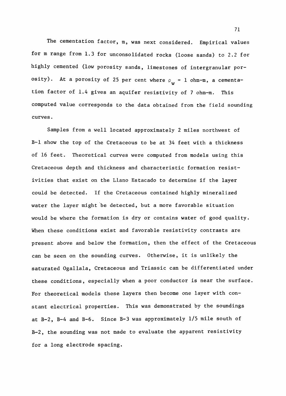
71
The cementation factor, m, was next considered. Empirical values
for m range from 1.3 for unconsolidated rocks (loose sands) to 2.2 for
highly cemented (low porosity sands, limestones of intergranular por
osity). At a porosity of 25 per cent where p = 1 ohm-m, a cementa-w
tion factor of 1.4 gives an aquifer resistivity of 7 ohm-m. This
computed value corresponds to the data obtained from the field sounding
curves.
Samples from a well located approximately 2 miles northwest of
B-1 show the top of the Cretaceous to be at 34 feet with a thickness
of 16 feet. Theoretical curves were computed from models using this
Cretaceous depth and thickness and characteristic formation resist
ivities that exist on the Llano Estacado to determine if the layer
could be detected. If the Cretaceous contained highly mineralized
water the layer might be detected, but a more favorable situation
would be where the formation is dry or contains water of good quality.
When these conditions exist and favorable resistivity contrasts are
present above and below the formation, then the effect of the Cretaceous
can be seen on the sounding curves. Otherwise, it is unlikely the
saturated Ogallala, Cretaceous and Triassic can be differentiated under
these conditions, especially when a poor conductor is near the surface.
For theoretical models these layers then become one layer with con
stant electrical properties. This was demonstrated by the soundings
at B-2, B-4 and B-6. Since B-3 was approximately 1/5 mile south of
B-2, the sounding was not made to evaluate the apparent resistivity
for a long electrode spacing.

72
Stations B-1 and B-5 show a slight increase in apparent resist
ivity with distance but these soundings do not give a complete cov
erage. At B-5 this increase in apparent resistivity is based only
on one reading at 200 feet and may not be reliable as indicated by
stations B-4 and B-6. At the northern end of the line, B-1 shows a
small but definite increase with electrode spacing. Although this
station has a maximum spacing of 80 feet and the increase is very
small, the field readings are deemed to be reliable due to the close
electrode spacing.
Since the infinite layer resistivities could be determined from
the sounding curves and depths to the top of this zone were known
from the water-table depths, it was then possible to determine the
model within the aerated zone. The basic shapes of sounding curves
B-1 through B-5 did not indicate an overburden of constant resistivity
above the water table, but more nearly a constant decrease in re
sistivities. Computed models with a constant rate of decrease did
not match the field data very well. Instead, a considerable portion
of the upper layer decreased rapidly and then was followed by a slow
decrease. In order to match the field sounding curves closely in some
cases, a low resistivity layer was needed below the shallow high re
sistivity layering.
Station B-7 gave a considerably different curve when compared
to the rest of the stations along Line B-B'. The subsurface model
shown on the cross section is one of a number of models that was found
to fit the curve reasonably well. This type of double-descending curve

73
with high apparent resistivities was characteristic of sounding data
obtained in the southeastern part of the area.
The computed models of Line B-B' show the lateral and vertical
variations that can be expected within the Ogallala. From the il
lustrated models it is seen that the Cretaceous was not detected and
is probably thin along most of the line. A thickening of the Cre
taceous section may occur near B-1, but this is not conclusive since
there may be a change within the Ogallala. This sounding was not ex
tended since the apparent resistivity changes were very small from
15 to 80 feet.
A limited resistivity contrast probably exists between the dry
and saturated Ogallala in the area. This lack of contrast may indi
cate a transition between the aeration and saturation zones. Although
there are considerable lithology and porosity changes in the vertical
section, there is indicated a general decrease in saturation of the
vertical section above the water table from B-1 through B-7.
The water table dips to the north from B-1 to B-6, contrary to
the regional dip of the water table on the Llano Estacado. It would
appear the values for water depths are reliable since the dip is con
stant between these stations. At B-5, B-6 and B-7 there is an in
crease in the resistivity of the infinite layer, although the value
at B-5 is based on only one point and may be unreliable. If changes
in resistivity and/or depth do occur in the Cretaceous and Triassic
at B-6 and B-7; these differences appear to be too great when the re
gional geology of the Cretaceous and Triassic is considered over a
distance of 2 miles. Therefore, a considerable change within the
Ogallala is probable.

74
Electric Log
The electric log (Plate IV) is from a Texas Water Development
Board test site located approximately 1 mile east of the southern
portion of Yellow Lake. A calibration was made to the nearest sounding
station at B-2 so that the asymptotic portions of a theoretical curve
at the well site and the field curve at B-2 would be equal. Interval
resistivities used to calculate the theoretical curves at the well site
were determined first by numerical integration using Simpson's rule
where b
y = / f(x)dx. a
A probable error exists in the computed interval resistivities as
various unknown bore-hole factors influencing the log readings were
not known. Also, the lack of penetrating power and a non-linear re
sponse from the single-point logging sonde did not permit an accurate
determination of the specific resistance of the formations.
For the formation resistivities above the fluid level in the hole,
selected values of 4.5 and 80.0 ohm-m were used to compute theoretical
soundings at the site. These two models show that at an electrode
spacing of 50 feet or more the apparent resistivities are nearly equal,
while at shorter spacings there is considerable change in the two
curves.
A Cretaceous section 24 feet thick with its top at a depth of
79 feet was determined from the well core. Two interval resistivities
of 4.0 and 5.0 ohm-m totaling 21 feet were used to represent this
section. When a 4.5 ohm-m upper layer resistivity was used in cal-

75
60 80 ohms m'/tn
f^
ELECTRICAL LOG
AND
IITED SOUNDING CURVES
PLATE 12
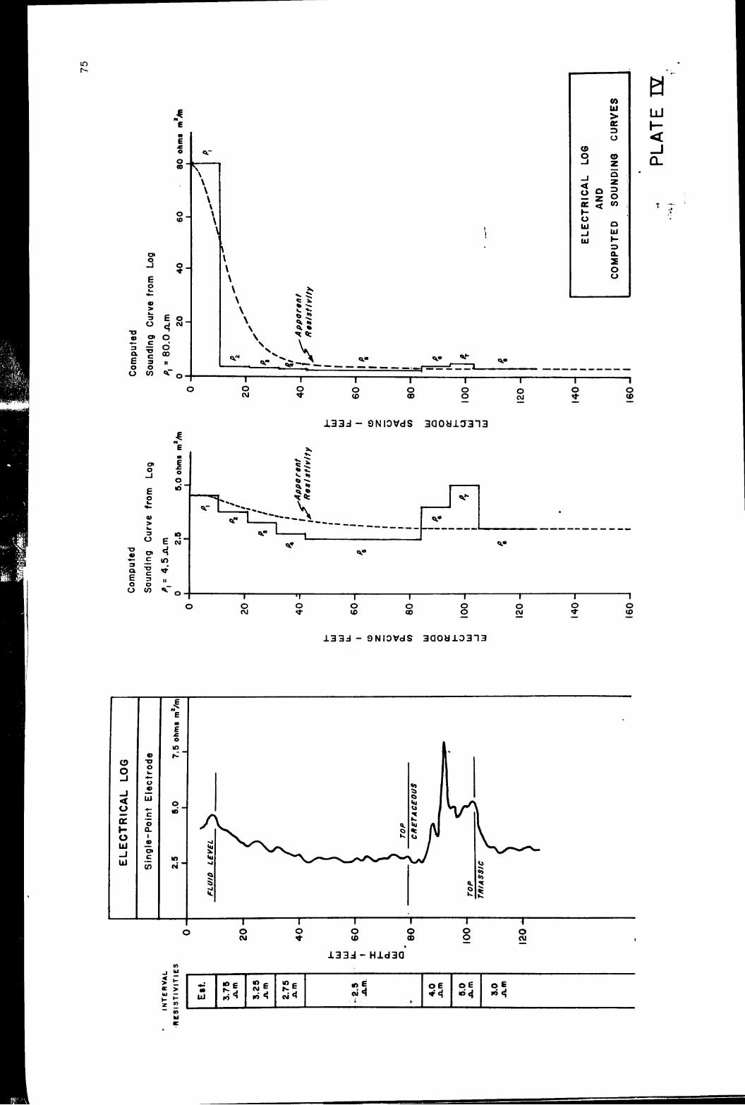
lO
3 E
o . CO
• o
« 3
a. b o u
o» o -1
E o &. ».— o > 3 o
a> c
c 3 o to
E < O
• o 00 II
«».
(C
o
o CM
r»
CO UJ
> 3 o
o q © -J z
_i ^
o o g — 2 S (C < OT ; K O _ UJ 9 _ j UJ UJ » -
3 a. Z o u
0 LU 1 -< .J O.
t
«*.• «*.•
o cvi
O o (0
o o o o cu
-r o o
(0
i 3 3 d - 9 N I 0 V d S 3a0aiJ313
«l • -
3 a t= a (J
a> o - I
E o t .
«»-w > ^ 3
o
o> c
•D
3 O OT
E < in «!f
«».
^ N E •• E
Oo
h
n
lO CM
n--^-.,S VlIZ «i.«
o CVJ
O 'I-
T " o o
00
o o o C\J
1 ^ o o
CO
1 3 3 d - ONIOVcJS 3 a o a i D 3 1 3
o o
< o Q : I -o UJ _ i UJ
a> o
« UJ
o 0 . I
— c en
E M
E e
lO 1 ^ '
o id
m CM
T " O
-r o o o
CM o (0
o o
i 3 3 d - Hl<J3a CO
5 E K >
UJ
n
•o CM •? CU S • i - .
O E o E

4f ^
76
culating a sounding curve, a minimum of 2.982 ohm-m occurred at an
electrode spacing of 110 feet and a second maxima of 3.034 ohm-m oc
curred at 290 feet. When an upper layer of poor conducting material
of 80.0 ohm-m was used, these critical points were reduced in amplitude
so as not to be observable by conventional field methods.
From the study of the well log, the previous conclusions about
the sedimentary section southeast of Yellow Lake were confirmed. With
in the upper part of the Ogallala, this log shows a definite decrease
in resistivities. The lower part of the Ogallala has a more constant
resistivity as illustrated by the previous electric log models com
puted for Line B-B'. Both the Cretaceous and Triassic resistivities
observed on the log were very nearly equal to those values predicted
from surface measurements.
On the basis of the well data it appears that both the Cretaceous
and Triassic dip to the south along Line B-B'. A favorable depth to
thickness ratio of the Cretaceous may influence the field curve at *,
B-1, while at B-2 and B-3 the curves are not influenced considerably
by this ratio. A smaller apparent resistivity for the infinite layer
at B-2 when compared to B-3 results from the increased depth to the
top of the Cretaceous at B-2.

CHAPTER XII
SUMMARY AND CONCLUSIONS
Theory and Computer Programming
Some mathematical preliminaries of the surface resistivity method
are discussed in Chapter II. Applications of the resistivity method
to ground-water problems in the Western hemisphere are reviewed in
Chapter III. Equations for a horizontally stratified earth were ex
tended to a maximum of eleven layers so the geology of the Llano
Estacado could be suitably represented. As indicated in Chapter IV,
the image analysis yielded mathematical expressions that were lengthy
and not suitable for hand calculations. These expressions were adapted
for use in a computer program so that apparent resistivity curves
could be computed rapidly.
Model Studies and Apparent Resistivity Curves
Average electrical properties of the Llano Estacado were evaluated
from the electric log and outcrop measurements as discussed in Chapter
VII. From the electrical resistivities of the shallow sedimentary
section, it was found that the section could be divided into three
overall units. These are as follows:
(1) Ogallala that varied considerably due to thin stringers
with varying degrees of porosity and lithology.
(2) Cretaceous that could be differentiated sometimes
from the overlying Ogallala.
77

78
(3) Triassic of considerable thickness with constant
resistivities.
A catalogue of apparent resistivity curves was prepared to rep
resent lithological and hydrological changes of the basic sedimentary
section described above. The effects of changes in resistivities,
thicknesses and depths are visually illustrated in the catalogue of
curves. Although the catalogue was designed primarily for use on the
Llano Estacado; it is readily adaptable to other areas, especially
when the resistivity contrasts are small. The exactness of these
curves makes it possible to interpolate with considerable accuracy
among the various models.
Survey in the Yellow House Canyon Area
Applications of the surface resistivity method on the Llano
Estacado are described in Chapter XI. The field data obtained in the
Yellow House Canyon area were closely related to the regional measure
ments made on the Llano Estacado.
Resistivity profiles, sounding data and an isoresistivity map
were interpreted. Theoretical values for water conductivities, degree
of saturation and porosities were used to demonstrate the reliability
of the sounding curves and related interpretation. Also, theoretical
sounding curves were computed from an electric log of an area test hole.
The resistivities obtained from this log compared favorably to the
theoretical resistivities that were computed from the sounding data
near the test site.
Much of the field data obtained in the area produced either de
scending or double-descending types of curves. These type curves re-
79
suited from a poor conducting material very near the surface and a
half space of low resistivity material. The rate of descent was con
trolled by the depth to the Triassic with changes in the double-de
scending curves attributed mainly to resistivity contrasts within the
Ogallala.
Prominent features of the isoresistivity map include the low ap
parent resistivities near the alkali lakes. The soundings indicate
considerable amounts of Cretaceous at or near the surface in the Bull
Lake area. Shallow water-saturated sands of high mineral content ap
pear to be present northeast of Bull Lake and in the vicinities of
Illusion and Yellow Lakes.
The two zones of low resistivity in the northern part of the
Illusion Lake area correspond to drainage systems into this lake.
Although separated by a topographic high, the apparent resistivities
indicate both Illusion and Yellow Lakes are in the same basin and this
basin area extends approximately four miles southeast of Yellow Lake.
High apparent resistivities were mapped on both sides of the basin
to the southeast.
A series of high resistivity anomalies were mapped in a north-
south direction through the central portion of the area and to the
southeast. These high resistivities result from considerable near-
surface caliche deposits in the area.
General Discussion
The material in this thesis brings together the aspects of theory,
computer programming and applications of the surface resistivity method
into a single analysis.

o
80
Certain field techniques were used to insure correct measurements
f the potentials. These accurate determinations were necessary before
any reliability in the interpretations could be made.
Changes in resistivities were observed by "jumps" in some of the
sounding curves. The differences between lateral variations and ver
tical changes were investigated on an experimental basis by using
Carpenter's tripotential method.
Eight basic types of curves were obtained from the regional field
data of the Llano Estacado. These were the same types as obtained in
the theoretical study.
Resistivity contrasts between the Triassic and overlying sediments
indicate the electrical boundary is equivalent to the top of the
Triassic in most places on the Llano Estacado. The physical and chem
ical characteristics of the Ogallala and Cretaceous are considerably
different based on a comparison of the lithological and electrical
sections above the Triassic.
Success of Surface Resistivity Measurements
The interpretation of apparent resistivities from surface methods
are usually dependent on curve matching techniques. With an increase
in the complexity of a section a unequivocal interpretation is not
possible without supporting evidence. Sound theoretical foundations,
accurate field measurements, and an intelligent combination of geo
physics and geology are necessary to translate these resistivity prop
erties into meaningful geology on the Llano Estacado.

81
LIST OF REFERENCES
Aldredge, R. F., 1937, The effect of dipping strata on earth resistivity determinations: Colorado School of Mines Quart., v. 32, no. 1, p. 169-186.
Archie, G- E., 1942, The electrical resistivity log as an aid in determining some reservoir characteristics; Am. Inst. Mining Metall. Trans., v. 146, p. 54-62.
Brand, J. P., 1953, Cretaceous of Llano Estacado of Texas: Bur. Econ. Geology, Texas Univ., Rept. Inv. 20, 59 p.
Buhle, M. B., and Brueckman, J. E., 1964, Electrical earth resistivity surveying in Illinois: Illinois Geol. Survey Circ. 376, 51 p.
Carpenter, E. W., 1955, Some notes concerning the Wenner configuration: Geophys, Prosp., v. 3, p. 388-402.
Cartwright, Keros, and McComas, M. R., 1968, Geophysical surveys in the vicinity of sanitary landfills in northeastern Illinois: Ground Water, v. 6, no. 5, p. 23-30.
Compagnie, Generale de Geophysique, 1955, Abaques de Sondage electrique: Geophys. Prosp., v- 3, supp. no. 3, 7 p.
Cronin, J. G., and Myers, B. M., 1964, A summary of the occurence and development of ground water in the southern High Plains of Texas: U. S. Geol. Survey Water-Supply Paper 1693, 88 p.
Depperman, K., 1954, Die Abhangigkeit des scheinbaren Widerstandes vom Sondenabstand bei der Vierpunktmethode: Geophys. Prosp., V. 2, p. 262-273.
Dudley, W. W., Jr., and McGinnis, L. D., 1962, Seismic refraction and earth resistivity investigation of hydrogeologic problems in the Humboldt river basin, Nevada: Desert Research Inst., Univ. of Nevada, Tech. Report No. 1.
Ehrenburg, D. 0., and Watson, R. J., 1932, Mathematical theory of electrical flow in stratified media with horizontal, homogeneous and isotropic layers: Am. Inst. Mining Metall. Engineers Trans., V. 97, p. 423-442.
Evans, G. L., 1949, Upper Cenozoic of the High Plains: West Texas and New Mexico Geol. Soc. Guidebook, Field Trip no. 2, p. 1-9.
Flathe, H., 1955, A practical method of calculating geoelectrical model graphs for horizontally stratified media: Geophys. Prosp., V. 3, p. 268-294.

82
1963, Five-layer master curves for the hydrogeological interpretation of geoelectrical resistivity measurements above a two-story aquifer: Geophys. Prosp., v. 11, p. 471-493.
Frye, J. C., and Leonard, A. B., 1957, Studies of Cenozoic geology along eastern margin of Texas High Plains, Armstrong to Howard Counties: Bur. Econ. Geology, Texas Univ., Rept. of Inv. no. 32, 62 p.
Grice, D. G., Green, Wilton, and Richardson, Wayne, 1965, Soil survey of Hockley County, Texas: Series 1961, No. 27, 65 p.
Hummel, J. N., 1929, Der scheinbare spezifische Widerstand bei vier pIan-parallelen Schichten: Zeitschr. Geophysik, v. 5, no. 5-6, p. 228-238.
Jakosky, J. J., and Wilson, C. H., 1934, Geophysical studies in placer and water supply problems: Eng. and Min. Jour., v. 135, p. 71-74.
Koefoed, 0., 1955, Resistivity curves for a conducting layer of finite thickness embedded in an otherwise homogeneous and less conducting earth: Geophys. Prosp., v. 3, p. 258-267.
Lancaster-Jones, E., 1930, The earth-resistivity method of electrical prospecting: Mining Mag., v. 42, no. 6, p. 352-355; v. 43, no. 1, p. 19-29.
Leggat, E. R. , 1957, Geology and ground-water resources of Lamb County, Texas: Texas Board of Water Engineers, Bull. 5704, 104 p.
Lotspiech, F. B., and Coover, J. P., 1962, Soil forming factors on the Llano Estacado: parent material, time and topography: Texas Jour. Sci., V. 14, p. 7-17.
Maillet, Raymond, 1947, The fundamental equations of electrical prospecting: Geophysics, v. 12, p. 529-556.
McFarland, H. F., 1962, Water is where you find it: Mines Magazine (Colorado), v. 52, no. 5, p. 12-15.
Mooney, H. M., and Wetzel, W. W., 1956, The potentials about a point electrode and apparent resistivity curves for a two-, three-, and four-layer earth: Minneapolis, Univ. of Minnesota Press, 146 p.
Newman, A. L., 1962, Soil survey of Lamb County, Texas: Series 1959, No. 7, 69 p.
O'Conner, R. E., and Bayne, C. K., 1959, Electrical resistivity studies in brine pollution problems: Symposium on Geophysics in Kansas, Kansas Geol. Sur. Bull. 137, p. 209-218.

83
Onodera, Seibe, 1960, The kernel function in the multiple-layer resistivity problem: Jour. Geophys. Research, v. 65, p. 3787-3794.
Orellana, Ernesto, 1963, Properties and drawing of the so-called Dar Zarrouk curves: Geophysics, v. 28, p. 99-110.
Page, L. M., 1968, Use of the electrical resistivity method for investigating geologic and hydrologic conditions in Santa Clara County, California: Ground Water, v. 6, no. 5, p. 31-40.
Roman, Irwin, 1934, Some interpretations of resistivity data: Am. Inst. Min. Metall. Engineers Trans., v. 110, p. 183-200.
Sayre, A. N., and Stephenson, E. L., 1937, The use of resistivity methods in the location of salt water bodies in El Paso, Texas, area: Am. Geophys. Union Trans., vol. 18, pt. 2, p. 393-398.
Schlumberger, Conrad, Schlumberger, Marcel, and Leonardon, E. G., 1934, Some observations concerning electrical measurements in anisotropic media, and their interpretation: Am. Inst. Mining Metall. Engineers Trans., v- 110, p. 159-182.
Sellards, E. H., Adkins, W. S., and Plummer, F. B., 1934, The geology of Texas, Vol. I, Stratigraphy: Bur. Econ. Geology, Texas Univ. Bull. 3232, 1007 p.
Slichter, L. B., 1933, The interpretation of the resistivity prospecting method for horizontal structures: Physics, v. 4, p. 307-322 and 407.
Stefanesco, S. S., Schlumberger, Conrad, and Schlumberger, Marcel, 1930, Sur la distribution electrique potentielle autour d'une prise de terre ponctue-le dans un terrain a couches horizontales humogenes et isotropes: Jour. Physique et Radium, ser. 7, v. 1, p. 132-141.
Swartz, J. H., 1937, Resistivity-studies of some salt-water boundaries in the Hawaiian Islands: Am. Geophys. Union Trans., v. 18, pt. 2, p. 387-393.
Tagg, G. F., 1934, Interpretation of resistivity measurements: Am. Inst. Min. Metall. Engineers Trans., v. 110, p. 135-147.
Unz, M., 1963, Relative resolving power of four-point resistivity configurations: Geophysics, v. 28, p. 447-456.
Van Dam, J. C., 1967, Mathematical denotation of standard-graphs for resistivity prospecting in view of their calculation by means of a digital computer: Geophys. Prosp., v. 15, p. 57-70.
Van Nostrand, R. G., and Cook, K. L., 1966, Interpretation of resistivity data: U. S. Geol. Survey Prof. Paper 499, 310 p.

84
Vincenz, S. A., 1968, Resistivity investigations of limestone aquifers in Jamaica: Geophysics, v. 33, no. 6, 1968, p. 980-994.
Warner, D. L. , 1969, Preliminary field studies using earth resistivity measurements for delineating zones of contaminated ground water. Ground Water, v. 7, no. 1, p. 9-16.
Watson, R. J., 1934, A contribution to the theory of the interpretation of resistivity measurements obtained from surface potential observations: Am. Inst. Mining Metall. Engineers Trans., v. 110, p. 201-236.
Wenner, Frank, 1915, A method of determining earth resistivity: U. S. Bur. Standards Bull., v. 8, p. 559-610.
Wetzel, W. W., and McMurry, H. V., 1937, A set of curves to assist in the interpretation of the three-layer resistivity problem: Am. Inst. Mining Metall., Engineers Trans., v. 2, p. 329-341.
White, W. H. , Broadhurst, W. L., and Lang, J. W., 1946, Ground water in the High Plains of Texas; U. S. Geol. Survey Water-Supply Paper 889-F, p. 381-420.
Wilcox, L. v., 1948, The quality of water for irrigation use: U. S. Dept. Agr. Tech. Bull. 962, p. 26.
Zohdy, A. A. R., 1965a, Earth resistivity and seismic refraction investigations near Santa Clara County, California: Ground Water, V. 3, no. 3, p. 41-48.
1965b, The auxiliary point method of electrical sounding interpretation, and its relationship to the dar Zarrouk parameters Geophysics, v. 30, no. 4, p. 644-660.

APPENDIX
CATALOGUE OF APPARENT RESISTIVITY CURVES
FOR THE WENNER CONFIGURATION
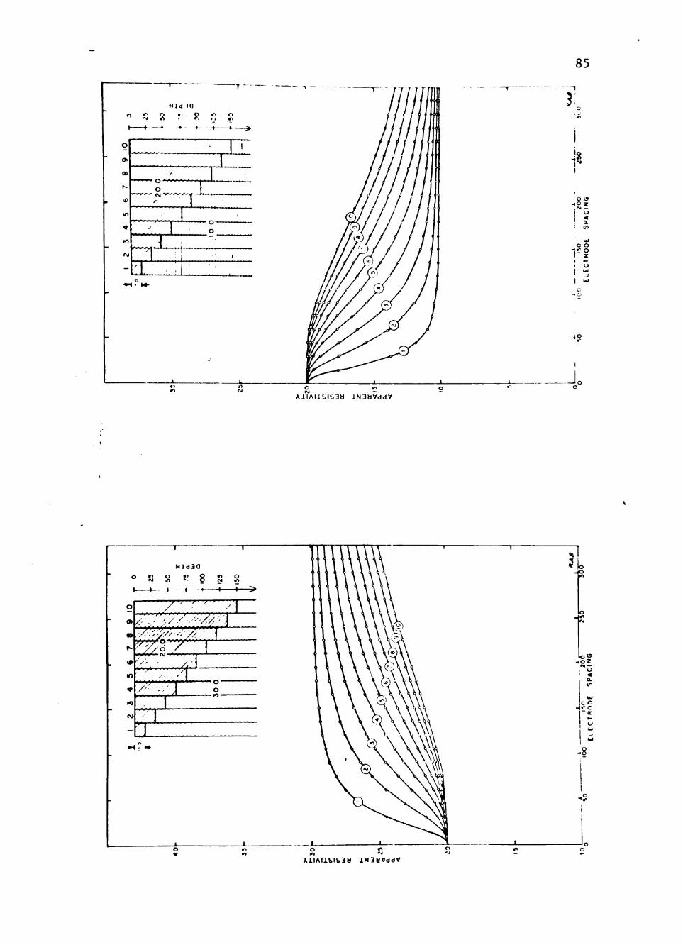
85
"T
H i d 10
" S 8 r ?. 1} I K —4 - • - * -•-
O r t
—•--
o>
<o
• o -o
J8 I
o o
:°-< in
c o I C O
-1°
J, X l l A I J S I s a U l N 3 U V d d «
Uld3Q
o o •A
—t—
n o « ^- O r j
- «»/•
-.4^5
/ ' :?
^^ i i , r , «n i < i^» i i > ' n ' » ' i
X' -"3
o
o
• / - ' ' ' 7]
o HO
4oz < — < a
c c •!•• c
AitAl i i>l i>3U l N 3 t t V d d V

86
H l d B Q O r>
o o>
OS
N
•
lO
r j
-
1—1
rt
$1 »i ft
g
o
r t
d
1 ^
1
' i 1
o '
1
'l
..i J
A1IAIXSIS3U l N 3 U V d d V
HidSO Q lO O in \ "-" f j o r- 1
M
— O
0>
a>
f-
(0
m
* •o
(M
-
oo^ OOfr
=:~bcv ^ ,6oc ^
0 oc
OOf \
ooe
0 0 2
0 0 2 '
• 0 0 1
! 0 0 1
' : 0 01
ooc 0 0 2
0 0 1
OOtF
0 0 2
lOOr
OOfr
OOC
| 0 0 1
0 0 *
ooc 0 0 2
A1IAI1SIS3« i N 3 a V d d *

87
to
N
o
(T
a>
f^
«> v>
* tn
<\t
-
'' / ,' /
''/'>' ///?
/. / '-' .'" /
./I
•' A-
/ • / , .
. . . ^ /.y.-:
• ' , ' ' ' • • '
occ ooc CC2
0 22
0 12
0 0 2
0 61
o e i
o« t
S2I
0 01
%L
OS
A1IAIXSIS3U IN3U«ddV
HldBO
° S 8 P I 1 ( 1 >
N
-o
0>
o
r-.
<o
m
•
•o
rg
-
0'5C
OOC
0 £2
0 0 2
C / l
OSI
a z i
o i l
oe S i
OS
S2
o
o o
g o
o < a.
o o ICO
IE
O • o
-Jo o
AJIAI1SIS3« IN38»ddV

88
Hid3a o *>. o
0)
» K
to
irt
V
•o
CM
-
0 0 *
OrSC
OT>C
0 9 2
OOZ
OSI
001
i l
ov
/
/;-
6 '
/
, ; /
Cl
Ai lA l lS ISaU IN3UVddV
ffl
CD
h-
«
lO
•
10
(M
-
0 0 *
OCC
ooc OC2
002
OCI
001
S i
OS
• ,
//
"4'^^. . 67
• / •
/ /- /
- o — 6
. 1 .
AllAl iSIS3b iN3UVddV

S:
Hid3Q
8 —4—
« i r
•
•>
N
-
X.^OOC v
ooc 0 0 2
- r yOOZ
0 0 1
1 0 0 1
' 0 0 2 / '
0 0 1
0-01
;ooc-.
ooc ' ^ 0 0 2 '
0 0 1
0 02
ooc 0 01
0 0 2
OOC
A l l A l i S l S 3 U l N 3 U V d d V
HXd30
1
(0
m
* m
CM
-
1 1
OOC
OOC
0 0 2
0 0 2
0 0 1
lOOl
- H 1
0 0 2
0 0 1
0 0 1
OOC
ooc 0 0 2
\ *
0 01
0 0 2
OOC
0 01^
0 0 2
OOC
A l l A l i S I S a H l N 3 U V d d V

90
HldSO
t—t—^
» ;
«;;
• s
« ;
rj P
— o
^ 0 01
^00?
i OOC
2 001
S 002
° OOC
A 1 1 A U S I S 3 M i N 3 « V d H V
A i l A l l S I S 3 H i N 3 U V d d V

AilAliSISaU i.N3UVddV
Hid30 (
0>
» N
« lO
•
K)
N
-
3 n rg
o n o e
.,2
5
•150
f
•
V V •" ^ ,
O >"v
lO ^
\
-
'
. / /.<'
^ l w < ^ o - ' / _
\
.i •',
y':V^y'
— . / ^ . . . . . . . / j ^ . . . . . . .
0.0
i
•¥*<•>*
o • o
o _ a. Z
•S i
-ii
AilAliSISaU INaUVddV

o
1
Hi.d3a O *t Q *>
«M B K
I 1 I I
2 CM
IT
O
9>
€0
K
W
n
*
10
CJ
" 6
•••• X
^ •
x^ -
0 .^
001
SI
09
X)S
o»
SC
^ S
sz
02
SI
fiz
OS
sz
1
d
1
;
AilAtiSIS3U i.N3(lVddV
Hid3a
S S S I > — f -
lO
N
— o
91
OD
N.
<t>
m
•
lO
N
-
••/•/ ' V
-'-•• 7 . y..- -.
'< • • / •
, . < ' / •
V / ' '
VrT^J^ V ,
^^;;y^ , > #
/ yy'.
/7Z-;
OOI
sx
0»
OS
0 *
sc
•o€
?z
102
61
fiZ
OS
rz
1
1
i
1
c
.
li l i •,'. 1
<3
C 3
I -
8 = A1IAIXSIS3U XN3UVddV

93
c
t
= o
<7t
CD
ID
* to
ni
-
H i d 3 0
"r 1
t "
•
10.0
•l
.1
o •*
^
9
rt
a s 5
1 I t
•t "l
ill ^ l l ' . i
ilill.
i l l ' I J ! ' • 1 ;
• 1 ,
i i j .
AXIAIXS1S3U XN3UVddV
HXd30 O o o n
lO
CSI
-O
«i
OD
K
« m
•
n
(M
1 • »
6
,
i i> i 1. 1
001
sx
09
X>i
0*
6 f
X)t
^Z
02
-fli
s;
OC
s-z
1 — >
~o—* 6
-X_
(Oo
°z
"Co
o -•o
_ o
AJ . IA IX6 I83U X N 3 b V d d V

'
94
Hid30 o ' o
1 1 ( 1
01
OD
K
<0
Irt
•
lO
<V1
-
,
O
- /
'
I ^
•
CsJ / /
.y/.'' 7'/ .^
— *
0.0
• < • * .
o : z <
- • - c a:
-8
J o
AX1AIXSIS3« X N 3 a V d d V
HXdBQ o "
9>
• r»
i «
m
lO
<M
1 \ ^
•?
"iJ I i 9
C4
l.<,
1
—o o
8
8?
a.
- C c
AXIAIXSIS3U XNSUVddV
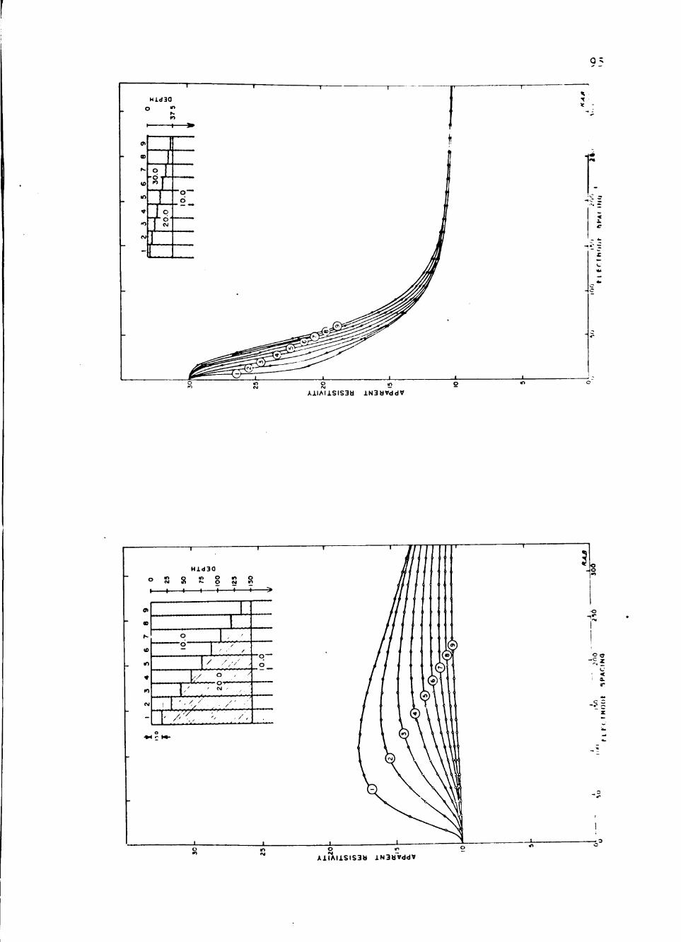
HXdiO
1 1
o
-T"o" J ~
10.0
1 1
U
AX1A1XS1S3U XN3UVddV
HXd30
o S 8 £ _ _ I 1 1 i ( +
o o M o
lO
01
OD
N
10
m
•
10
p j
-
1 o o
, '
I - . ' , V ,
__k 1 ' . /
' yy'
// ° ,' ^ ' CM ^ ^
/ / / ^ •
o
o - o
•o
1
-II • <
a.
AXIA IXS IS3b XNSUVddV

96
AXIAIXS1S3U XN3UVddV
AXIAIXSIS3t ) XN3t lVddV

97
HXdSO O « O
t
<r>
00
K
10
o
<t
lO
PJ
-
1 1 1 —
30
0
N
1
; o o
. » . • 1 1
/ ''
->
/' y
/..
T-O
v 6 y.
/ / •'
/ •
'/ //.
/ .
AXIAIXSIS3U XN3UVddV
HXdSa O « o
0>
CD
K
(0
in
•
10
CJ
-
M O 1
^ \
. \l s «. r
, J ' l . s '
• i ' ' '1 ,1,
\
b x\
^ \ ^ '• , s
•< : : • •
A X I A I I S I S 3 U XN3U«ddV

95
HXd3a O »> O if> S <n Q to m '~ 9 N n
I 1 • 1 1 « 1-
^
T j O . ; 4 iig'i I - o
51 o
. o . n ^ ^
A. n f^**
z
ICC r • — u
-i
AXIAIXSIS3U XN3tiVddV
o
HXd3a o m
n Q m O r- O <sj in
-H 1 1 1 -
\ '' /
, , , , ; , ' : M
, ''!
1
• ^
X /
! • ! '
- o q :, CJ '
H' '"'•'' 1
F
OO
C
\
^ •
-
•'• / V
1 ' \ ^
Hf l - t J
•3 o • o
-8?
^
JO
A X I A I X S I S a u XN3tJVddV

99
MXd3G o
»— 2 r o O r^ ri -* 1 f-
K
<0
in
* (O
CJ
-
" p 6
1 o -1 o
/ •
1
1
0.0
1
* o
u < a.
sla'
AX1A1XSIS38 X N 3 U V d d V
—lo o
N X d 3 0
K<i *H
- ^
<
OD
r
10
m
* lO
(M
-
> m r j s lO
100
1
3 3
"*t"••
/ ' ^ - • '
• 15
0
•/y
• ' - ' / • ^ ; > / ' '
' lo ' ,/. X
'H
. . - / •
• - ^ A • /
c c
> >
1
kXI>IX
"f o
I
< ' a.
o o I t / O
a
c - o
iO
S1S3H XN3UVddV

1C3
AXlA IXS lS3d XN3UVddV
HXd30
1 1——1 1 1 1 1 -^
—o-d
— lO -
y
.^ /
20.0
f
/
' '• / •
A
/ ' / •
/
/'/ 1
o o
t
' 1
? ,
• c z
r.
jz
AXIAIXSIS3M X N 3 a V d d V

101
AXIAIXSIS3U XN3UVddV
HXd3a o
I—
to o o m o
to m
(O
r j
•< rw --r/) 1—
° '\''yy • *
/yyy<^o<y<y-z
-M. '.y/y.^'/-
• . 1 ^ M-
^ o
-8
IO I —
u <
«%o
u
AXIAIXSlS3ti XN3UVddV

i c : 1 —I
H idSO o ' " o r > p r > o
'M »> - 9 5? 5
« 1 1 K
10
- C.
-
1 1 o
O CJ
*
1
o
<»•
1
AXIAIXSIS38 XNSaVddV
HXd30 « o » o
•' ' l O
o *o,-
I 9 -ro*
'! I
w-s* *
3:
^ ; z I <
1 • •
o in AXI^IXSIS3U XN3UVddV

103
o
HXdSa
o
to
zz o
o>
OD
in
* fO
<M
-
i
ij
OO
I-
1 ,1
$
Si •1 N ci fO
•ri
o
s o ri in
O
<3i
1 ,
o — o —
_ o _
• H t k
I '
AXIAIXSIS3U XN3UVddV
A i l A I X S I S 3 U l N 3 U V d d V

K
HXd30 o n o n
1
to
~ o
at
w
10
in
«• ") to
-
^ 1 T 5 ^
' I ' '
i •
U t 1-
''
*
10.0
t
! . ' •
ix' 1 1 1
1 XL
i 1
*
s » N
to
rt
rt
O in
»J
p
6
1 •
.' i \'\ • \
1 10
0
!
:
—... I
_ ^ . -" *— ..*...
• o ' • .
::::;:
:::n3
*! IT U
; * •";
- K 2 *+s» -
JJ£
c -
AXIAIXSIS3U XN3UVddV
AXIAIXSIS3U XN3UVddV

105
H i d 3 a r> o
(VJ
-o
0>
OD
I--
<0
IO
* lO
Ol
-
10.0
o
« S d
r> rJ 6 eg
.0.
IS
n
c> r>
r> cvi
p
r) d
•
. 1
00
$ K>
o to S
. 0.
O IO
m rj O
O
10.0
o
—ri —
+ p r i AXIAI1S1S3U XN3UVddV
HXd3a n o
CJ
Z
o
0)
»
(0
in
•
(O
(M
-
1 1 1 1 >
OO
I
c
« lO o
O to
SI 1 01
r>
Q
in ni
o
m d
10
0
d
d m
!!J d
2
o
o in
p
•n d
10
0
/
, . . y .
o - o ^
-' ^ ' • > / /
/"
/ •
AXIAIXSIS3U i N 3 U V d d V

106
MXd3a
° S 8 P I — I — I — » -
CJ
-o
0>
CD
(0
m
t
ro
OJ
-
10.0
'
- L
d
n
8 t4
O
r>
d
o r)
"1 Ci
O
d
o o
1,
•l ;
M J
0.5
o
1
o rt
,5.
.0.
d CJ
r> CJ
d
o c
10.0
r:.
o — i n " "
_1_
AXIAIXS1S3U XN3UVddV
HXd30
OJ
— o
0>
a>
<0
n
•
lO
OJ
-
1 • 1 1 i ^ ^
20.0
o
r>
o
ci CJ
o
r i
d
K O ri
p
•a o
o O
1
d
<> d
id ni
6
o 10 J>
O
•9 <?
o o
. . ; . . !
:;;::;
o - •
111 IT"
- - - "
o o
f j £ u 41
: o oc
u UJ
H ° U -
AXIAIXSIS3U lN3MVddV

107
AXIAIXSIS3« XN3MVddV
HXd3a
8 in o CJ m
H 1 1 1-
O
OD
• . X ^ S \ ; . \ x - • • • •>• ' • > » >•:••><:'•>
,. .. . .R:x- x-i • " ^ ^ . r x - IVx X
-^<''^X o •/• I't' •t^>;'/' • tM
>/'-,
^•O: iitia • H S M -
AXIAIXSIS3t l XN3UVddV

•^ n z
AXlAIXSIS3b XN3«VddV
o
» —
HXd3G O n r> • .
H 1
'I- f /v .' • <.' ' y 'y '" ' = • . • / • • . • • • : ; - > : - X / ^ : - . . :
:^?:-<iJ^--4:-S:x ' iftA »yyr^<;.,.,...,4 t m^. , . - . . . , l . :>.-; . / / , .
CO
CJ
••S:;-;i4<^
y-'4-/yy<:< / y . '• /.
^ ^ ; - - - ^ ^:r>^<>-
A X I A I X S I S 3 H XN3UVddV
