a theory of anharmonic lattice statics for analysis … elasticity (2007) 86:41–83 doi...
TRANSCRIPT

J Elasticity (2007) 86:41–83DOI 10.1007/s10659-006-9079-8
A Theory of Anharmonic Lattice Staticsfor Analysis of Defective Crystals
Arash Yavari · Michael Ortiz · Kaushik Bhattacharya
Received: 10 October 2005 / Accepted: 19 August 2006 /Published online: 27 October 2006© Springer Science + Business Media B.V. 2006
Abstract This paper develops a theory of anharmonic lattice statics for the analysisof defective complex lattices. This theory differs from the classical treatments ofdefects in lattice statics in that it does not rely on harmonic and homogenous forceconstants. Instead, it starts with an interatomic potential, possibly with infinite rangeas appropriate for situations with electrostatics, and calculates the equilibrium statesof defects. In particular, the present theory accounts for the differences in the forceconstants near defects and in the bulk. The present formulation reduces the analysisof defective crystals to the solution of a system of nonlinear difference equations withappropriate boundary conditions. A harmonic problem is obtained by linearizing thenonlinear equations, and a method for obtaining analytical solutions is described insituations where one can exploit symmetry. It is then extended to the anharmonicproblem using modified Newton–Raphson iteration. The method is demonstratedfor model problems motivated by domain walls in ferroelectric materials.
Key words lattice statics · defective crystals · discrete mechanics
Mathematics Subject Classification (2000) 74A25
1 Introduction
The method of lattice statics introduced by Born and his co-workers (see [5]) hasbeen widely used to study various aspects of atomistic solids. In particular, it has
A. Yavari (B)School of Civil and Environmental Engineering, Georgia Institute of Technology,Atlanta, GA 30332, USAe-mail: [email protected]
M. Ortiz · K. BhattacharyaDivision of Engineering and Applied Science, California Institute of Technology,Pasadena, CA 91125, USA

42 J Elasticity (2007) 86:41–83
been widely used to study equilibrium structure of defects. Based on a formulationin [23] and [30], this version of lattice statics has been used for point defects in [15]and [18], for interstitial in [17], for cracks in [12] and [22], for surfaces in [16] and fordislocations by [6, 12, 13, 28, 35] and [37]. Further reviews can be found in [6, 8, 18–20, 25, 29, 33–36, 38] and references therein. This method considers a harmonicdefect-free crystal subjected to an eigendeformation chosen to represent the defect.The advantages of the method are that they provide analytic solutions and that theydo not require any ad hoc cut-off or periodicity assumptions. However, they areharmonic and homogeneous, and importantly do not account for the strong nonlinearand heterogeneous behavior near the defect core. It should also be mentioned thatnone of the above-mentioned works solve the defect problem as a discrete boundary-value problem. In contrast, nonlinear treatments of defects are overwhelminglycomputational and restrict themselves to finite domains or periodicity assumptions.
This paper is concerned with the formulation of a semi-analytical method ofsolution of fully nonlinear lattice statics problems for defective crystals. In particular,the method of solution takes as input an arbitrary interatomic potential, and is notrestricted to interactions based on harmonic force constants. The solutions obtainedrepresent equilibrium configurations for the input interatomic potential. The methodof solution is based on a modified Newton–Raphson iteration. Each step in theiteration requires the solution of a harmonic problem with uniform force constants.The uniformity of the force constants ensures that methods of solution for differenceequations, such as the discrete Fourier transform, can be applied to the linearizedproblem. The out-of-balance forces are computed from the full interatomic potential,thus ensuring that converged solutions represent equilibrium configurations of theanharmonic crystal. The iteration starts from a nominal configuration of the defectivecrystal. This initial configuration is not in equilibrium in general and the correspond-ing out-of-balance forces are not zero. The main purpose of the initial configuration isto place the crystal in the energy well corresponding to the defect of interest. Generalresults then ensure that if the equilibrium defect is stable, i.e., if the correspondingforce constants are coercive, and the initial nominal defect is sufficiently close to theequilibrium defect, the modified Newton–Raphson iteration converges linearly.
We demonstrate our methodology using a model problem motivated by the studyof domain walls in ferroelectric perovskites. Elsewhere we present detailed results ofdomain walls and defects on domain walls using more widely accepted potentials.
This paper is organized as follows. Section 1 reviews harmonic lattice statics. Wereformulate lattice statics in a language as close to continuum mechanics as possible.In Section 2 the idea of symmetry reduction for defective crystals is presentedand some subtleties in the linearized discrete governing equations are explained.Section 3 presents the idea of anharmonic lattice statics. Solution techniques forsolving the linearized discrete governing equations are explained in Section 4. InSection 5 our formulation of lattice statics is generalized to a system of dipoles inwhich interactions are pairwise but not isotropic and atom position vectors are notthe only degrees of freedom. The method of solution is illustrated by means of severalexamples concerned with the equilibrium structure of 180◦ and 90◦ domain wallsin a two-dimensional lattice of dipoles. Conclusions are given in Section 6. In theAppendix we show that with little modification our approach can be applied to three-body interactions.

J Elasticity (2007) 86:41–83 43
2 Discrete Governing Equations
Consider a collection of atoms L and assume that they interact through someinteratomic potentials. Let xi denote the position of atom i ∈ L and Si the set (list)of other atoms that it interacts with. We prohibit self interaction by assuming i /∈ Si.The total energy is a function of the atomic positions,
E = E({x j} j∈L
), (1)
and we assume that this may be written as the sum of the energy per atom
E =∑
i∈LE i (xi, {x j} j∈Si
). (2)
Note that this partitioning of energy cannot be done unambiguously in general.However, this is unambiguous in the case of pairwise interactions. Assuming thatthere are no discrete body forces, equilibrium requires1
∂E∂xi
= 0 ∀i ∈ L. (4)
It can be easily shown that this is equivalent to equilibrating energy of the atom E i
with respect to xi, i.e.,
∂E i
∂xi
(xi, {x j} j∈Si
) = 0. (5)
These Eqs. 4 and 5 embody the main idea behind lattice or molecular statics. We
seek a solution to Eq. 5 close to a given reference configuration B0 =(
xi0, {x j
0} j∈Si
).
Therefore we expand the governing Eq. 5 about this reference configuration:
∂E i
∂xi= ∂E i
∂xi(B0) + ∂2E i
∂xi∂xi(B0) (xi − xi
0) +∑
j∈Si
∂2E i
∂x j∂xi(B0) (x j − x j
0) + ... = 0. (6)
We obtain the harmonic approximation by dropping the higher order terms.It can be easily shown that because of translation invariance of the potential
∂2E i
∂xi∂xi(B0) = −
∑
j∈Si
∂2E i
∂x j∂xi(B0) . (7)
This is trivially verified for pair-wise interactions and shown in the Appendix tohold for three-body interactions. Using this, we rewrite the harmonic lattice staticsequations to be
∑
j∈Si
∂2E i
∂x j∂xi(B0) (x j − x j
0) −∑
j∈Si
∂2E i
∂x j∂xi(B0) (xi − xi
0) = −∂E i
∂xi(B0) . (8)
1When there is a discrete field of body forces this is written as
− ∂E i
∂xi
(xi, {x j} j∈Si
)+ Fi = 0. (3)

44 J Elasticity (2007) 86:41–83
Setting
fi = −∂E i
∂xi(B0) ,
ui = xi − xi0,
Kij = ∂2E i
∂xi∂x j(B0) , (9)
the harmonic lattice statics governing equations may be written as
∑
j∈Si
Kij(u j − ui) = fi ∀ i ∈ L. (10)
A couple of remarks are in order. The matrix of force constants Kij are derivedfrom a potential about some reference configuration, and thus they depend on thereference configuration. In particular, they may depend explicitly on the indices iand j. In the classical formulation of harmonic lattice statics, the governing equationswould be written for some periodic lattice and the force constants would depend onlyon the reference distance between atoms i and j.
The unbalanced force field f = {fi}i∈L can be written as
fi =∑
j∈LKij�u j
e ∀ i ∈ L. (11)
Or
f = T (�ue), (12)
where the field of eigen-deformations �ue = {�uie}i∈L is formally defined as
�ue = T −1(f). (13)
Thus we can rewrite Eq. 10 as
∑
j∈LKij
(u j − �u j
e
) = 0 ∀ i ∈ L (14)
and recognize it to be exactly that as the classical equation of harmonic lattice stat-ics [34].
2.1 Linearized Discrete Governing Equations for Defective Crystalswith No Symmetry Reduction
We now specialize to a (defective) complex lattice with a unit cell consisting of Natoms. Here by “defective” lattice we mean a collection of atoms that is locally like aperfect complex lattice. We index the unit cells using integers (m, n, p) ∈ Z
3. LetIαβγ denote the Ith atom in the (α, β, γ ) unit cell. Given an atom i, any other

J Elasticity (2007) 86:41–83 45
atom j can be specified uniquely by the unit cell it belongs to and its type, i.e.,j = Iαβγ . The discrete harmonic governing equations (10) can now be written as
∞∑
α,β,γ=−∞′
N∑
I=1
KiIαβγ
(uI
αβγ − ui) = fi ∀ i ∈ L, (15)
where the prime on the summation means that the self-interaction term has beenexcluded.
Let us define unit cell displacement vectors as
Umnp =⎛
⎜⎝
u1mnp...
uNmnp
⎞
⎟⎠ (m, n, p) ∈ Z
3. (16)
Now the discrete governing equations can be written in terms of interaction of unitcells as
∞∑
α,β,γ=−∞Aαβγ (m, n, p)Um+α,n+β,p+γ = Fmnp (m, n, p) ∈ Z
3, (17)
where
Aαβγ (m, n, p) ∈ R3N×3N, Um+α,n+β,p+γ , Fmnp ∈ R
3N . (18)
This is a linear vector-valued partial difference equation with variable coefficientmatrices of infinite order. The unit cell force vectors and the unit cell stiffnessmatrices are defined as
Fmnp =⎛
⎜⎝
F1mnp...
FNmnp
⎞
⎟⎠ ,
Aαβγ (m, n, p) =
⎛
⎜⎜⎜⎝
K11αβγ K12αβγ · · · K1Nαβγ
K21αβγ K22αβγ · · · K2Nαβγ
...... · · · ...
KN1αβγ KN2αβγ · · · KNNαβγ
⎞
⎟⎟⎟⎠
. (19)
To be able to solve such a difference equation one needs to assume a finite rangeof interaction and then numerically study the effect of the range of interaction.Assuming ranges of interaction r1, r2 and r3 in m, n and p directions, respectively,we have
r1∑
α=−r1
r2∑
β=−r2
r3∑
γ=−r3
Aαβγ (m, n, p)Um+α,n+β,p+γ = Fmnp (m, n, p) ∈ Z3, (20)
which is a linear partial difference equation of order r = max(2r1, 2r2, 2r3).

46 J Elasticity (2007) 86:41–83
2.2 Linearized Discrete Governing Equations for Defective Crystalswith 2-D Symmetry Reduction
Let us now consider a complex lattice with a defect that is extended in one dimensionso that we can reduce the problem to two dimensions. In other words, we study acollection of atoms which have translation invariance in only one direction. In orderto do so, we note that such a complex lattice may be written as the disjoint union ofone dimensional complex lattices:
Ld2 =
⊔
α,β∈Z
Ld2(α, β), (21)
where Ld2(α, β) is a one-dimensional lattice or mathematically an equivalence class
of atoms. Each one-dimensional complex lattice is a chain of unit cells. Becauseeach unit cell is equivalent to any other unit cell in the chain, the decomposition(21) can be thought of as a partitioning of the defective complex lattice into someequivalence classes (chains). Choosing a representative from each equivalence classLd
2(α, β), the resulting two-dimensional lattice is called the reduced lattice and isdenoted by Ld2 . Further the neighboring set Si can be partitioned as
Si =⊔
α,β∈Z
N⊔
I=1
SIαβ(i), (22)
where SIαβ(i) is an equivalence class of equivalent atoms which all would have thesame displacement with respect to a given reference configuration. In other words,SIαβ(i) is the set of atoms of type I in the chain Ld
2(α, β) that interact with atom i. Anexample would be a lattice with broken atomic bonds on a half plane, i.e., a crack. Inthis example equivalence classes are sets of atoms lying on lines parallel to the crackedge (front). With this partitioning one can write
∑
j∈Si
Kiju j =∞∑
α,β=−∞′
N∑
I=1
KiIαβ uIαβ, (23)
where
KiIαβ =∑
j∈SIαβ (i)
∂2E i
∂xIαβ∂xi(B0) , (24)
and prime on the summation means that the self-interaction term has been excluded.It is seen that in a defective lattice there is a partial symmetry and a given atom iinteracts with equivalence classes and this is why each substiffness matrix is definedin terms of a lattice sum. Thus the discrete governing equations can now be written as
∞∑
α,β=−∞′
N∑
I=1
KiIαβ
(uI
αβ − ui) = fi ∀ i ∈ L. (25)
J Elasticity (2007) 86:41–83 47
Let us define unit cell displacement vectors as
Umn =⎛
⎜⎝
u1mn...
uNmn
⎞
⎟⎠ . (26)
Now the governing equations can be written in terms of interaction of unit cells as
∞∑
α,β=−∞Aαβ(m, n)Um+α,n+β = Fmn (m, n) ∈ Z
2, (27)
where
Aαβ(m, n) ∈ R3N×3N, Um+α,n+β, Fmn ∈ R
3N . (28)
This is a linear vector-valued partial difference equation with variable coefficientmatrices in two independent variables. The unit cell force vectors and the unit cellstiffness matrices are defined as
Fmn =⎛
⎜⎝
F1mn...
FNmn
⎞
⎟⎠ ,
Aαβ(m, n) =
⎛
⎜⎜⎜⎝
K11αβ K12αβ · · · K1Nαβ
K21αβ K22αβ · · · K2Nαβ
...... · · · ...
KN1αβ KN2αβ · · · KNNαβ
⎞
⎟⎟⎟⎠
. (29)
2.3 Linearized Discrete Governing Equations for Defective Crystalswith 1-D Symmetry Reduction
We now consider a collection of atoms that has translation invariance in twodirections. In other words, L is a collection of two-dimensional perfect lattices. Thuslet us assume that L can be partitioned into two-dimensional equivalence classes:
Ld1 =
⊔
α∈Z
Ld1(α) (30)
or infinite sets of atoms Ld1(α) that lie on some planes. Each Ld
1(α) is a two-dimensional periodic collection of unit cells, i.e., a perfect two-dimensional complexlattice. Choosing a representative from each equivalence class,the resulting chain iscalled the reduced lattice Ld1 . The neighboring set Si can be partitioned as
Si =⊔
α∈Z
N⊔
I=1
SIα(i), (31)
where SIα(i) is the equivalence class of all the atoms of type I and index α withrespect to atom i. In other words, SIα(i) is the set of all atoms of type I in the twodimensional lattice Ld
1(α) that interact with atom i. For a domain wall, for example,each equivalence class is a set of atoms lying on a plane parallel to the domain wall.

48 J Elasticity (2007) 86:41–83
With this partitioning one can write the linearized discrete governing equations as
∞∑
α=−∞′
N∑
I=1
KiIαuIα +
(
−∞∑
α=−∞′
N∑
I=1
KiIα
)
ui = fi, (32)
where the prime on the first sum means that the term α = 0, I = i is excluded to avoidself-interaction and
KiIα =∑
j∈SIα(i)
∂2E i
∂x j∂xi(B0),
fi = −∂E i
∂xi(B0),
uIα = xIα − xIα
0 = x j − x j0 ∀ j ∈ SIα(i). (33)
Let us define unit cell displacement vectors as
Um =⎛
⎜⎝
u1m...
uNm
⎞
⎟⎠ . (34)
Now the governing equations can be written in terms of interaction of unit cells as
∞∑
α=−∞Aα(m)Um+α = Fm m ∈ Z, (35)
where
Aα(m) ∈ R3N×3N, Uα, Fm ∈ R
3N . (36)
This is a linear vector-valued ordinary difference equation with variable coefficientmatrices. The unit cell force vectors and the unit cell stiffness matrices are defined as
Fm =⎛
⎜⎝
F1m...
FNm
⎞
⎟⎠ , Aα(m) =
⎛
⎜⎜⎜⎝
K11α K12α · · · K1Nα
K21α K22α · · · K2Nα
...... · · · ...
KN1α KN2α · · · KNNα
⎞
⎟⎟⎟⎠
. (37)
Note that, in general, Aα(m) need not be symmetric as will be explained shortly. Theabove system of difference equations is a Volterra system of difference equations(see [11]).2
2Lattice statics analysis of defective crystals with 1-D symmetry reduction leads to the solution ofvector-valued ordinary difference equations with variable coefficient matrices. Inhomogeneities arelocalized and the idea is to treat the inhomogeneous region as boundary and transition regions.This will result in two vector-valued difference equations with constant coefficient matrices oneforward and one backward. In the end, the original difference equation will be solved by matchingthe solutions of these two ordinary difference equations.

J Elasticity (2007) 86:41–83 49
The above governing equations can be written in terms of a discrete convolutionoperator as3
AX = F, (38)
where X = {Xn}, F = {Fn} and the discrete convolution operator is defined as
AX = {(AX
)n
}, (39)
and
(AX)n =∞∑
m=−∞An−mXm. (40)
2.4 Some Remarks
For the case of N ≥ 2, there are some subtleties in calculating the Aα matrices.This is also the case for defective crystals with 2-D and no symmetry reductions butfor the sake of simplicity we explain this subtlety only for defective crystals with a1-D symmetry reduction. One subtlety is that some interactions should be ignored.One is the interaction of an atom of type I and index n with all atoms of type Iand index n, i.e., there are no interactions within a given equivalence class (this is aconsequence of Eq. 7). This means that A0 has a special structure. When positionof atom i of type I changes, all its equivalent atoms, i.e., those with α = 0 undergothe same perturbation. Atoms of the same type as i do not contribute to energy ofi because the potential is pairwise and their relative distances from the atom i arealways the same. This means that
KI I0 = −∞∑
α=−∞′
N∑
J=1J �=I
KI Jα. (41)
The same thing is true for forcing terms. The reason for this is that the distancebetween the equivalent atoms is fixed and atoms in the equivalence class of i do notcontribute to − ∂E i
∂xi and its derivatives. For a defective crystal with a 2-D symmetryreduction the above property implies that
KI I00 = −∞∑
α,β=−∞′
N∑
J=1J �=I
KI Jαβ . (42)
The other subtlety is when a finite number of interactions is considered forrepresentative unit cells. Consider atoms with index n and project the whole defectivecrystal on a line perpendicular to the two-dimensional defect. This would be thereduced lattice Ld1. As an example, we have the picture shown in Figure 1 for Aand O2 atoms in a perovskite mutilattice ABO3. Suppose a given representativeunit cell interacts with its first mth nearest neighbor (representative) unit cells. We
3This is the approach that [2] chooses in his treatment of difference equations. We do not use thisnotation in this paper but it would be useful to know that the discrete governing equations have adiscrete convolution form.

50 J Elasticity (2007) 86:41–83
Figure 1 Nearest neighbors ofA and O2 atoms and theirindices in an ABO3 defectivecrystal with a 1-D symmetryreduction.
consider the interaction of A and O2 atoms with other A and O2 atoms of indices{n − m, ..., n + m} (except the ones that have already been excluded). Looking atFigure 1, one can see that symmetry of interactions dictates that interactions of Aand O2 atoms with O1, O2 and O3 atoms with index n + m should be ignored.Similarly, consider atoms B, O2 or O3 with index n and their nearest neighbors asshown in Figure 2. Every atom B (O1 or O3) interacts with B, O1 and O3 atoms withindex {n − m, ..., n + m} (except the ones that have already been excluded). Again,symmetry implies that the interactions of B, O1 and O3 atoms with A and O2 atomswith index n − m should be ignored.
Another interesting subtlety is the symmetry of Aα matrices. It should be notedthat each KiIα is symmetric but the matrices Aα (α = −m, ..., m) are not symmetric,in general. This can be seen more clearly in a simple 2-D model. Consider a 2-Drectangular multi-lattice composed of two simple lattices each with lattice parametersa and c and the shift vector p = (p1, p2). This system has three coefficient matricesA-1,A0,A1 ∈ R
4×4. We now compare K12-1 and K21-1 to see if A-1 is symmetric. Itcan be easily shown that
K12-1 =∑
Y{n−1}
∂2 E∂xn−1∂yn−1
(B0) , (43)
K21-1 =∑
X{n−1}
∂2 E∂yn−1∂xn−1
(B0) , (44)
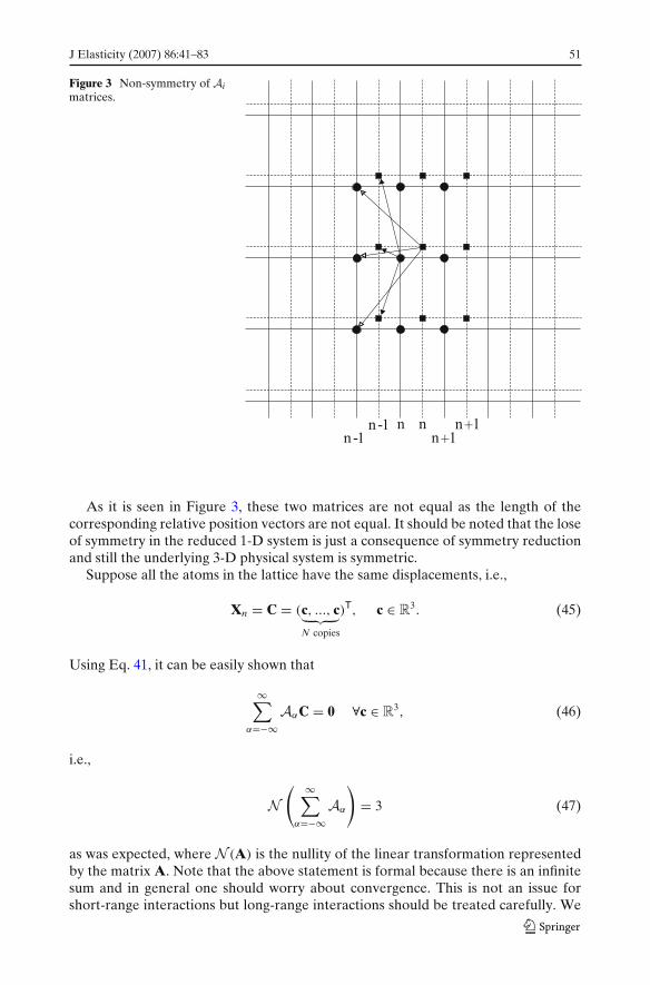
where X{n − 1} is the set of atoms of type 1 which have index n − 1 relative to theatom n of type 2 (these are the circles in Figure 3). Similarly, Y{n − 1} is the set ofatoms of type 2 which have index n − 1 relative to the atom n of type 1 (these are thesquares in Figure 3). xn−1 and yn−1 are position vectors of atoms of types 1 and 2 withindex n − 1, respectively.
Figure 2 Nearest neighbors ofB, O1 and O3 atoms and theirindices in an ABO3 defectivecrystal with a 1-D symmetryreduction.
J Elasticity (2007) 86:41–83 51
Figure 3 Non-symmetry of Aimatrices.
As it is seen in Figure 3, these two matrices are not equal as the length of thecorresponding relative position vectors are not equal. It should be noted that the loseof symmetry in the reduced 1-D system is just a consequence of symmetry reductionand still the underlying 3-D physical system is symmetric.
Suppose all the atoms in the lattice have the same displacements, i.e.,
Xn = C = (c, ..., c︸ ︷︷ ︸N copies
)T, c ∈ R3. (45)
Using Eq. 41, it can be easily shown that
∞∑
α=−∞AαC = 0 ∀c ∈ R
3, (46)
i.e.,
N( ∞∑
α=−∞Aα
)
= 3 (47)
as was expected, where N (A) is the nullity of the linear transformation representedby the matrix A. Note that the above statement is formal because there is an infinitesum and in general one should worry about convergence. This is not an issue forshort-range interactions but long-range interactions should be treated carefully. We

52 J Elasticity (2007) 86:41–83
will come back to the convergence issue in the sequel. For the case of a defectivecrystal with a 2-D symmetry reduction the above property states that
N
⎛
⎝∞∑
α,β=−∞Aαβ
⎞
⎠ = 3. (48)
There is another symmetry relating A−γ to Aγ . It can be easily shown thatreciprocity implies that
KI J−γ = KJIγ . (49)
This means that
A−γ = ATγ . (50)
Convergence of infinite sums raise their own delicate issues. In the analysis ofdefective crystals with 1-D and 2-D symmetry reductions, we need to calculatestiffness matrices that are defined in terms of lattice sums of square matrices. Discretefield of unbalanced forces is also defined in terms of lattice sums. Since we will beinterested in dipole–dipole interactions, we will find that substiffness matrices fordefective crystals with 1-D and 2-D symmetry reductions are absolutely convergent.However, the forces are obtained as conditionally convergent sums and thus requirecare. In our examples, we look at systems of dipoles lying on a plane and thus forceis also defined in terms of absolutely convergent lattice sums.
Finally, our lattice statics model forces are always calculated exactly. However, tobe able to solve the governing discrete equations for an infinite lattice we need tohave a system of difference equations of finite order. It would be interesting to knowhow sensitive the solutions are to the range of interaction of representative unit cells.This is problem dependent and should be carefully studied for a given interatomicpotential.
In all the existing lattice statics calculations a fixed number of nearest neighborinteractions (usually only the first and second nearest-neighbor interactions) areconsidered. Our formulation of lattice statics can consider any number of nearest-neighbor interactions and this enables us to numerically study the effect of rangeof interactions with no difficulty. In Section 5 we present a numerical study of theeffect of range of interaction for a lattice of dipoles. It will be seen that the effectivepotential is highly localized and increasing the range of interaction does not changethe displacements, i.e., the displacements are independent of the range of interaction.
Our formulation of anharmonic lattice statics starts with choosing a referenceconfiguration. Here a comment is in order regarding the choice of reference con-figuration. For a given defect, reference configuration is chosen to be a nominaldefect. By ‘nominal’ defect, we mean a configuration that is locally like the bulkcrystal but in some region(s) is close to the relaxed configuration of the defect.Of course, a nominal defect is not unique. An example is shown in Figure 4 foran edge dislocation. In this figure we show the reduced lattice, i.e., representativeatoms of lines of atoms perpendicular to the plane. We know that a dislocation canbe understood as an extra half plane of atoms inserted in the bulk lattice (in thereduced lattice a half line of extra atoms). Figure 4a shows a nominal defect that hasbeen obtained by inserting a half plane of extra atoms between two crystallographicplanes. In Figure 4b the configuration (a) has been modified to make it exactly like

J Elasticity (2007) 86:41–83 53
Figure 4 Two possible reference configurations for a dislocation.
the bulk crystal except in the region bounded by the broken lines. These two nominaldefect reference configurations are both acceptable choices but configuration (b)is preferable because its unbalanced force field is localized and this makes thenumerical calculations more efficient.
In the previous lattice statics models of dislocations [6, 20, 28] always some cuttingand pasting process is used. In the present formulation all is needed is a referenceconfiguration. The unit cell numbering for an edge dislocation is shown in Figure 5.Note that the n-axis is ‘curved’ but still the governing linearized equations are
∑
α,β
Aαβ(m, n)Xm+α,n+β = Fmn (m, n) ∈ Z2. (51)
We close this section by stating our harmonic lattice statics algorithm:
Input data: defective crystal geometry, interatomic potential� Initialization
� Construct B0, calculate force and substiffness matrix moduli� Do for all α ∈ K
s
� Assemble substiffness matrices and construct Aα
� End Do
� Calculate unbalanced forces F0 = F(B0)
� Solve the governing linear difference equations� End

54 J Elasticity (2007) 86:41–83
Figure 5 Unit cell numberingfor the reference configurationof an edge dislocation.
3 Anharmonic Lattice Statics
The classical harmonic lattice statics is not appropriate where displacements from theinitial configuration are large. There have been modifications of the harmonic latticestatics in the past [12, 13, 20]. The idea of these and similar works is to considerthe fully nonlinear equations close to defects. These works, however, do not solve anonlinear defect problem as a discrete boundary-value problem; instead all these andsimilar works are more or less heuristic. In this section we present a formulation ofanharmonic lattice statics in which one solves a nonlinear discrete defect problem bysolving discrete linear boundary-value problems. Anharmonic lattice statics is basedon Newton–Raphson (NR) method for solving nonlinear equations. The basic ideaof NR method is to look at a quadratic approximation to the nonlinear equations ineach step. Suppose f : R
n → Rn is continuously differentiable and that f(x∗) = 0 for
some x∗ ∈ D ⊂ Rn. We know that derivative of f is a linear map defined as
f(x + u) = f(x) + Df(x)u + o(‖u‖). (52)
Let us start from an initial guess x0 ∈ D. The linear approximation of f about x0
calculated at a point x1 ∈ D is
f(x1) ≈ f(x0) + Df(x0)(x1 − x0). (53)
Assuming that f(x1) ≈ 0 we have
x1 = x0 − Df(x0)−1f(x0). (54)
Similarly, in the kth step
xk+1 = xk − Df(xk)−1f(xk). (55)
It can be shown that this algorithm has a quadratic convergence (see [10]), i.e.,
‖xk+1 − x∗‖ ≤ C‖xk − x∗‖2 for some positive number C. (56)
The modified NR method is based on a similar idea. In the kth iteration one defines
xk+1 = xk − Df(x0)−1f(xk), (57)
i.e., the only difference is that in all the steps the derivative of the initial guess is used.This is however slower than the usual NR iteration.

J Elasticity (2007) 86:41–83 55
By modifying the proof presented in [10], it can be shown that the convergence ofmodified NR method is linear, i.e.,
‖xk+1 − x∗‖ ≤ c‖xk − x∗‖ for some c ∈ (0, 1). (58)
The idea of anharmonic lattice statics is to find the nonlinear solutions by amodified Newton–Raphson iteration. In modified Newton–Raphson method theHessian matrix is not updated in each iteration and the initial Hessian is used.Modified Newton–Raphson method is slowly and linearly convergent and a largenumber of iterations should be performed to get good results. In our lattice staticscalculations this is an efficient method as the most expensive part of the calculationsis the computation of substiffness matrices (very slowly converging lattice sums). Itis important to note that the Hessian at x = x0 should be positive–definite for themodified NR to converge to a local minimum of the energy.
Here we explain the idea for all three types of defective crystals. Let α ∈ Z3, Z
2, Z
for defective crystals with no symmetry reduction, with a 2-D symmetry reductionand with a 1-D symmetry reduction, respectively. The linearized governing equationshave the following form
∑
α∈Zs
AαUn+α = Fn n ∈ Zs (s = 1, 2, or 3). (59)
Note that in general Aα = Aα(n) and are evaluated with respect to a given referenceconfiguration B0. Given a reference configuration B0, we calculate the discretefield of unbalanced forces exactly. Let us denote this by F0 = {F0
n}n∈Zs . Note thatF0 : Lds → R
3, where Lds is the reduced defective lattice.4 Having F0, one has thefollowing discrete boundary value problem (DBVP)
∑
α∈Zs
AαU0n+α = F0
n n ∈ Zs
Boundary Conditions (B.C.) (60)
The boundary conditions are problem dependent. For infinite defective crystals werequire boundedness of displacements at infinity. Solving the above DBVP oneobtains U0 = {U0
n}n∈Zs . Now the reference configuration is updated as follows.
B10 = B0 + U0. (61)
In the case of a system with B0 = {X0n}n∈Zs , i.e., when the only degrees of freedom are
position vectors of the lattice points, this means that{X1
n
}n∈Zs = {
X0n + U0
n
}n∈Zs . (62)
Now having a new reference configuration one can calculate the discrete field ofunbalanced forces F1 = {F1
n}n∈Zs . In the second step one has the following DBVP∑
α∈Zs
AαU1n+α = F1
n n ∈ Zs
B.C. (63)
4In the case of a defective crystal with no symmetry reduction Ld3 = L.

56 J Elasticity (2007) 86:41–83
Note that the stiffness matrices are not updated and in all the steps the originalstiffness matrices are used. Solving the above DBVP one obtains U1 = {U1
n}n∈Zs andB2
0 = B10 + U1. This process at step k requires solving the following BVP
∑
α∈Zs
AαUk−1n+α = Fk−1
n n ∈ Zs
B.C. (64)
where
Fk−1 = F(Bk−10 ) and Bk−1
0 = Bk−20 + Uk−2. (65)
Depending on the problem the fields Uk are localized or localized modulo somerigid translation fields. This means that the fields Fk are localized. This is problemdependent and one should carefully study the rate of decay of unbalanced forces fora given defective crystal. The following is our anharmonic lattice statics algorithm:
Input data: B0,Aα, U0
� Initialization
� B10 = B0 + U0
� Do until convergence is achieved
� Fk = F(Bk0 )
� Calculate Uk by solving the harmonic problem� Bk+1
0 = Bk0 + Uk
� End Do� End
4 Solution Methods for the Linearized Discrete Governing Equations
In this section we present analytic methods for solving the discrete governingequations for defective crystals with 1-D, 2-D and no symmetry reductions. Inanharmonic lattice statics the first step in solving a nonlinear problem is to solvethe linearized governing equations. Linearized governing equations with respect to agiven reference configuration are vector-valued partial difference equations. In thissection we briefly review the theory of ordinary and partial difference equations.
4.1 Theory of Difference Equations
Difference equations arise in many problems of mathematical physics. They alsoappear in discretization of boundary value problems and also in combinatorics.In this subsection we review a few facts and theorems from theory of differenceequations. For more details see [1, 11, 26] and references therein.

J Elasticity (2007) 86:41–83 57
4.1.1 Ordinary Difference Equations
An ordinary difference equation is the discrete analogue of an ordinary differentialequation. Difference equations can be defined on bounded or unbounded discretedomains. For us all difference equations are defined on unbounded domains. Con-sider a sequence {un}n∈N ⊂ R. A difference equation in the independent variable n isan equation of the form
f (n, un, ..., un+p) = 0. (66)
The order of a difference equation is the difference between the largest and smallestarguments explicitly involved in the equation. A linear (scalar-valued) differenceequation has the following form
p∑
j=0
K j(n)un+ j = bn n ∈ N. (67)
Here, we are interested in linear difference equations with constant coefficients.These equations show up in discrete systems with uniform physical properties.Consider a pth order difference equation with constant coefficients
un+p + a1un+p−1 + a2un+p−2 + ... + apun = bn. (68)
Similar to differential equations, one first solves the corresponding homogeneousequation. Assuming that solutions are of the form λn, λ ∈ C, one obtains
λp + a1λp−1 + ... + ap = 0. (69)
This is the characteristic polynomial of the difference equation (68). There areseveral possibilities for characteristic roots. If all the roots are real and distinct, forexample, the general solution is of the form
ucn = c1λ
n1 + c2λ
n2 + ... + c1λ
np. (70)
For details on other possibilities see [11]. The general solution of Eq. 68 can bewritten as
un = ucn + up
n , (71)
where upn is a particular solution of the nonhomogeneous equation.
58 J Elasticity (2007) 86:41–83
A system of linear difference equations of first order has the following form5
un+1 = A(n)un + bn, un, bn ∈ Rp, A(n) ∈ R
p×p, n ∈ N ∪ {0}. (73)
If A does not depend on n the system (73) is called a system with constantcoefficients.
un+1 = Aun + bn. (74)
For the homogeneous system with constant coefficients corresponding to Eq. 74, i.e.,
un+1 = Aun (75)
the general solution is
un = Anc, c ∈ Rp, ∀n ∈ N. (76)
Here, An is called the fundamental matrix of the system (74). This is the analogue ofeAt in a linear system of differential equations. System of difference equations (74)has p linearly independent solutions and the general solution can be written as
un = Anc + upn , (77)
where upn is a particular solution. Using the method of variation of constants the
general solution can be expressed as
un = Anc +n−1∑
j=0
An− j−1b j. (78)
Note that a system of difference equations can be thought of as a vector-valuedordinary difference equation.
4.1.2 Partial Difference Equations
Partial difference equations are discrete analogues of partial differential equations.Let Z
p be the set of all p-tuples of integers (p ≥ 2). A linear partial differenceequation has the following form
LXα =∑
β∈�
A(β)Xα+β = Fα, (79)
where � ⊂ Zp, α, β ∈ Z
p and
X, F : � → Rq, A : � → R
q × Rq. (80)
5It should be noted that this is not the most general form of a linear vector-valued difference equa-tion. The most general first-order linear vector-valued difference equation has the following form
A1(n)un+1 + A2(n)un = bn, un, bn ∈ Rp, A1(n),A2(n) ∈ R
p×p, n ∈ N ∪ {0}. (72)
The matrix A1 can be singular in general. A direct solution of this equation in the case of constantcoefficient matrices can be found in [42].

J Elasticity (2007) 86:41–83 59
For p = 2, a linear partial difference equation has the following form
∑
(r,s)∈Z2
ArsXm+r,n+s = Fmn (m, n) ∈ �. (81)
It is known that [21] solution space of a partial difference equation is, in general,infinite dimensional. This means that explicit solutions of partial difference equationscannot be as simple as those of ordinary difference equations. The most commontechniques for solving linear partial difference equations are integral transforms.For solving partial difference equations on bounded rectangular domains there aredirect methods using matrix tensor product methods [27]. However, these methodsare not applicable to the problems we have in mind for defective crystals. Thereare also some direct methods for solving simple partial difference equations (see[32]). However, these methods are not applicable for general vector-valued partialdifference equations.
4.1.3 Discrete Fourier Transform
Discrete Fourier Transform (DFT) is a powerful technique for solving systems oflinear difference equations. In the literature there are two different types of discreteFourier transform both known as DFT. The first type, which is the one we use inthis paper, transforms a sequence (or more precisely a lattice function) to a functionof a continuous variable(s). This is sometimes called continuous discrete Fouriertransform (CDFT). Theory of CDFT was developed in [2, 3, 41]. The other typeof DFT, which we call discrete DFT (DDFT), transforms a sequence to anothersequence [4, 7] and is usually useful for solving periodic difference equations ordifference equations on bounded domains. We will briefly review DDFT and itsapplications in solving difference equations with periodic boundary conditions at theend of this section. In this work by DFT we mean CDFT, i.e., the one that maps alattice function to a continuous function in k-space.
Consider a lattice L and a lattice function f : L → R3. The discrete Fourier
transform of f is defined formally as
f (k) = V∑
j∈Lf ( j )eik·x j
k ∈ B, (82)
where V is the volume of the unit cell and B is the first Brillouin zone. For a chainof atoms of unit lattice spacing this definition reduces to the usual definition of DFTof a sequence in R, where V = 1, B = [−π, π ]. Let us denote by U the set of alldiscrete Fourier transformable lattice functions. Let us also denote by R the set ofthose lattice functions such that
| f (x)| ≤ C3∏
i=1
(1 + |xi|p) ∀ x = (x1, x2, x3) ∈ L, (83)
for some integer p ≥ 0 and constant C ≥ 0. It can be shown [41] that there is a one-to-one correspondence between the spaces R and U . It should be noted that in thedefinition of DFT the convergence should be understood in the sense of distributions.

60 J Elasticity (2007) 86:41–83
Inverse DFT is defined as
f ( j) = 1
(2π)3
∫
Bf (k)e−ik·x j
d3k. (84)
DFT has many nice properties and here we mention a few of them. DFT is a linearoperator, i.e.,
(α f + βg)∧ = α f + β g ∀α, β ∈ R, ∀ f, g ∈ U . (85)
Shifting property of DFT is essential in solving difference equations. Suppose
Xn = Y(k). (86)
Then
Xn+m = e−im·k Y(k). (87)
Discrete convolution of two lattice functions f and g is defined as
( f ∗ g)(i) = V∑
j∈Lf (i − j )g( j ). (88)
Note that the multiplication f (i − j)g( j) is defined componentwise. If f, g ∈ U ,then
(f ∗ g
)(k) = f (k)g(k). (89)
Discrete Fourier Transform is a powerful tool in solving partial difference equationsbut should be used carefully in numerical calculations as the integrands in inverseDFT may be extremely oscillatory.
4.1.4 DFT and Difference Equations
Consider the following ordinary difference equation.
xp+1 − 2xp + xp−1 = fp p ∈ Z. (90)
Note that this difference equation is translation invariant, i.e., if the sequence {xp}p∈Z
is a solution so is the sequence {xp + c}p∈Z, ∀ c ∈ R. Applying DFT to this differenceequation we obtain
(e−ik − 2 + eik) xp(k) = fp(k). (91)
Or
xp(k) = 1
2(cos k − 1)fp(k). (92)
Thus formally
xp = 1
2π
∫ π
−π
e−ipk 1
2(cos k − 1)fp(k)dk. (93)

J Elasticity (2007) 86:41–83 61
Note that this integral is not convergent in general because there is a singularity atk = 0, i.e.,
1
2(cos k − 1)= − 1
k2+ O(1). (94)
This is a consequence of translation invariance of the difference equation. In otherwords for this difference equation the solution can be obtained up to a rigid transla-tion and this shows up in the inverse discrete Fourier transform as a singularity. Onecan make the integral convergent by adding a suitable rigid translation. The followingwould be a rigid translation that removes the singularity.
xp = 1
2π
∫ π
−π
e−ipk[
1
2(cos k − 1)fp(k) − eipk
2(cos k − 1)
]dk. (95)
For R-valued difference equations there are rigorous treatments of this problemin the literature (see [9] and [40]). In a special case when the loading sequenceis symmetric about p = 0 the inverse DFT is convergent. An example would bethe following.
f−p = fp ∀ p ∈ N, f0 = 0. (96)
In this case fp(0) = 0 and the inverse DFT is convergent.Consider the following linear vector-valued partial difference equation with con-
stant coefficient matrices.r1∑
α=−r1
r2∑
β=−r2
r3∑
γ=−r3
Aαβγ Um+α,n+β,p+γ = Fmnp (m, n, p) ∈ Z3. (97)
Taking DFT from both sides of the above equation, we obtain
Z(k)Umnp(k) = Fmnp(k) k ∈ B = [−π, π ]3, (98)
where
Z(k) =r1∑
α=−r1
r2∑
β=−r2
r3∑
γ=−r3
e−i(αk1+βk2+γ k3)Aαβγ (99)
is the symbol of the difference equation. Assuming that Z(k) is invertible in B thesolution can be written as
Umnp = 1
(2π)3
∫
Be−im·kZ−1(k)Fmnp(k) dk, (100)
where m = (m, n, p). Symbol of a difference equation is not invertible, in general.An example would be singularity of the symbol at k = 0 for a translation-invariantdifference equation. Assuming that origin is the only singularity point, solution ofthe difference equation can be obtained by imposing a suitable rigid translation. Thefollowing is a suitable choice.
Umnp = 1
(2π)3
∫
Be−im·k [Z−1(k) − eim·kD(k)
]Fnmp(k) dk, (101)

62 J Elasticity (2007) 86:41–83
where
D(k) =⎛
⎜⎝
U(k) . . . U(k)...
...
U(k) . . . U(k)
⎞
⎟⎠ , U(k) =
⎛
⎝d1(k) 0 0
0 d2(k) 00 0 d3(k)
⎞
⎠ ,
d1(k) = (Z−1(k)
)11 , d2(k) = (
Z−1(k))
22 , d3(k) = (Z−1(k)
)33 . (102)
An alternative approach to remove the singularity is as follows. Let us firstintroduce the following change of variables
Umnp = (−1)m+n+p Umnp, Fmnp = (−1)m+n+p Fmnp, Aαβγ = (−1)α+β+γ Aαβγ . (103)
The governing equations in terms of the new variables are
r1∑
α=−r1
r2∑
β=−r2
r3∑
γ=−r3
Aαβγ Um+α,n+β,p+γ = Fmnp (m, n, p) ∈ Z3. (104)
The above system of difference equations is not translation invariant. As an example,let us look at the difference equation (90). Defining xp = (−1)pxp and fp = (−1)p fp,the difference equation is rewritten as
−xp+1 − 2xp − xp−1 = (−1)p fp p ∈ Z. (105)
It is seen that this equation is not translation invariant. The solution of the originaldifference equation can be written as
xp = (−1)p
2π
∫ π
−π
e−ipk
2(i sin k − 1)
fp(k)dk. (106)
4.1.5 Difference Equations on Finite Domains: Periodic Boundary Conditions
In any numerical treatment of defects in crystals, e.g., molecular dynamics, ab initiocalculations, etc., one takes a supercell large enough to be a representative of thedefective crystal and then extends it to the whole space periodically. A useful tool forsolving difference equations with periodic boundary conditions is the discrete DFT.Here we explain some of its details for applications to ordinary difference equations.But the results can be extended to partial difference equations with no difficulty.
Consider a function f : I → R, where I = {0, 1, ..., N − 1}, N ∈ N and f is peri-odic, i.e.,
f (m + kN) = f (m) ∀ k ∈ Z. (107)
f can be thought of as a finite sequence with N elements. Discrete DFT of f isdefined as
f (k) =N−1∑
m=0
f (m)ωmkN ∀ k ∈ I, (108)

J Elasticity (2007) 86:41–83 63
where ωN = e− 2π iN . The inverse of discrete DFT has the following representation
f (n) = 1
N
N−1∑
n=0
f (k)ω−nkN ∀ n ∈ I. (109)
For a sequence {xn}N−1n=1 it can be easily shown that
xn+1(k) = ω−kN xn(k) + ω−k
N (xn − x0) . (110)
Similarly
xn−1(k) = ωkN xn(k) + x−1 − xN−1. (111)
Let us consider the following discrete boundary-value problem
xn+1 − αxn + xn−1 = fn n = 0, 1, ..., N − 1,
x0 = xN (x−1 = xN−1). (112)
Taking DFT from both sides one obtains
Z (k)xn(k) = fn(k), (113)
where Z (k) = ωkN + ω−k
N − α. Thus
xn(k) = Z (k)−1 fn(k) (114)
and hence
xn = 1
N
N−1∑
k=0
Z (k)−1 fn(k)ω−nkN n ∈ I. (115)
This would be the solution sequence as long as Z (k) �= 0. Suppose α = 2, e.g., thegoverning equation of a chain of atoms with harmonic interactions between nearestneighbors. In this case the difference equation is translation invariant and henceZ (0) = 0. In Eq. 115 let us remove the k = 0 term and define
xn = 1
N
N−1∑
k=1
Z (k)−1 fn(k)ω−nkN n ∈ I. (116)
Note that
xn − xn = 1
NZ (0)−1
N−1∑
m=0
fm, (117)
which is a constant, i.e., xn is equal to xn up to a rigid translation. Note also that if thesystem is self-equilibrated, i.e., if
∑N−1m=0 fm = 0 then the singularity of Z (k) at k = 0
causes no problem.Let us now consider a vector-valued difference equation and define DFT compo-
nentwise. Thus for Xn ∈ Rd define
Xn(k) =N−1∑
m=0
ωmkN Xm n ∈ I. (118)

64 J Elasticity (2007) 86:41–83
Therefore one can show the following two relations easily.
Xn+1(k) = ω−kN Xn(k) + ω−k
N (XN − X0) , (119)
Xn−1(k) = ωkNXn(k) + X−1 − XN−1. (120)
Consider the following discrete boundary-value problem with a periodic boundarycondition.
A−1Xn−1 + A0Xn + A1Xn+1 = Fn n = 0, ..., N − 1,
XN = X0, X−1 = XN−1. (121)
Taking DFT from both sides and using the boundary conditions, formally one has
Xn(k) = Z(k)−1Fn(k) (122)
and hence
Xn = 1
N
N−1∑
k=0
Z(k)−1Fn(k)ω−nkN n = 0, ..., N − 1, (123)
where Z(k) = ωkNA−1 + A0 + ω−k
N A1. Note that for a translation-invariant differenceequation Z(0) is singular and the solution is obtained by removing the term k = 0.
5 Lattice Statics Analysis of a Defective Lattice of Point Dipoles
In this section we consider a two-dimensional defective lattice of dipoles with latticeparameter a. Each lattice point represents a unit cell and the corresponding dipoleis somehow a measure of the distortion of the unit cell with respect to the highsymmetry phase. This system is interesting in the sense that its potential energy is notonly a function of atom (unit cell) positions; it depends on polarization vectors too.This means that the potential energy is partially translation invariant. Total energyof the lattice is assumed to have the following three parts
E({xi}i∈L, {Pi}i∈L
) = Ed ({xi, Pi}i∈L)+ E short ({xi}i∈L
)+ Ea ({Pi}i∈L), (124)
where Ed, E short and Ea are the dipole energy, short-range energy and anisotropyenergy, respectively. These energies have the following forms. The first term is
Ed = 1
2
∑
i, j∈Lj�=i
[Pi · P j
|xi − x j|3 − 3Pi · (xi − x j) P j · (xi − x j)
|xi − x j|5]
+∑
i∈L
1
2αPi · Pi, (125)

J Elasticity (2007) 86:41–83 65
where α is the electric polarizability and is assumed to be the same for all thelattice points (molecules).6 The short-range energy is modelled by a Lennard–Jonespotential with the following form
E short = 1
2
∑
i, j∈Lj�=i
4ε
[(a
|xi − x j|)12
−(
a|xi − x j|
)6]
. (126)
The anisotropy energy quantifies the tendency of the lattice to remain in some energywells. We assume the following form for this energy
Ea =∑
i∈LKA|Pi − P1|2 ...|Pi − Ps|2. (127)
This means that the dipoles prefer to have values in the set {P1, ..., Ps}. Note that thisis a self-energy.
Let S = ({xi}i∈L, {Pi}i∈L)
be the equilibrium configuration (a local minimum of theenergy), i.e.,
∂E∂xi
= ∂E∂Pi
= 0 ∀ i ∈ L. (128)
Linearizing the governing equations (128) about a reference configuration B0 =({xi0}i∈L, {Pi
0}i∈L)
we obtain
∂E∂xi
(B0) + ∂2E∂xi∂xi
(B0) (xi − xi0) +
∑
j∈Si
∂2E∂x j∂xi
(B0) (x j − x j0)
+ ∂2E∂Pi∂xi
(B0) (Pi − Pi0) +
∑
j∈Si
∂2E∂P j∂xi
(B0) (P j − P j0) + ... = 0, (129)
∂E∂Pi
(B0) + ∂2E∂xi∂Pi
(B0) (xi − xi0) +
∑
j∈Si
∂2E∂x j∂Pi
(B0) (x j − x j0)
+ ∂2E∂Pi∂Pi
(B0) (Pi − Pi0) +
∑
j∈Si
∂2E∂P j∂Pi
(B0) (P j − P j0) + ... = 0, (130)
where Si is the neighboring set of atom i. Note that the only contribution to theterm ∂2E
∂Pi∂Pi (B0) comes from the anisotropy energy and the polarizability part of thedipole–dipole energy and has the following form for the case of s = 27
Kpp0 := ∂2E
∂Pi∂Pi(B0)
= 2KA(|Pi
0 − P1|2 + |Pi0 − P2|2
)I + 4KA
(Pi
0 − P1)⊗ (
Pi0 − P2
)
+ 4KA(Pi
0 − P2)⊗ (
Pi0 − P1
)+ 1
αI, (131)
6Note that the last part of this energy is a self-energy.7But note that Kpp
0 has contributions from dipole–dipole interactions.
66 J Elasticity (2007) 86:41–83
where I is the 2 × 2 identity matrix and ⊗ denotes tensor product. Assuminginteractions of order m, for a defective crystal with a 1-D symmetry reduction theset Si can be partitioned as follows
Si =m⊔
α=−m
N⊔
I=1
SIα(i), (132)
where SIα(i) is the set of atoms of type I lying on the line parallel to the y-axis andαa away from the atom i.8 Let us define
ui = xi − xi0, qi = Pi − Pi
0, (133)
fxi = − ∂E
∂xi(B0) , fp
i = − ∂E∂Pi
(B0) , (134)
and
KxxiIα = δα0
∂2E∂xi∂xi
(B0) +∑
j∈SIα(i)
∂2E∂x j∂xi
(B0) ,
KxpiIα = δα0
∂2E∂Pi∂xi
(B0) +∑
j∈SIα(i)
∂2E∂P j∂xi
(B0) ,
KpxiIα = δα0
∂2E∂xi∂Pi
(B0) +∑
j∈SIα(i)
∂2E∂x j∂Pi
(B0) ,
KppiIα = δα0Kpp
0 +∑
j∈SIα(i)
∂2E∂P j∂Pi
(B0) . (135)
With the above definitions the linearized governing equations can be written as
m∑
α=−m
N∑
I=1
KxxiIαuI
α +m∑
α=−m
N∑
I=1
KxpiIαqI
α = fxi , (136)
m∑
α=−m
N∑
I=1
KpxiIαuI
α +m∑
α=−m
N∑
I=1
KppiIαqI
α = fpi . (137)
Now by simply looking at the linearized equations, one would expect to seetranslation-invariance for the variable uI
α . This means that the sum of matrices thatact on uI
α cannot be full rank, i.e., in R2
N(
m∑
α=−m
N∑
I=1
KxxiIα
)
= N(
m∑
α=−m
N∑
I=1
KpxiIα
)
= 2 (138)
Note that this is not the case for matrices that act on qIα variables.
One should note that dipole–dipole energy is pairwise but not isotropic. In otherwords, the energy is the sum of pairwise interaction of dipoles but for each pair
8Here we have assumed that each unit cell has N dipoles and the defect lies on the line x = 0.
J Elasticity (2007) 86:41–83 67
the energy is not only a function of the relative distance of dipoles; in addition torelative distances it depends on the dot product of the relative position vectors andthe polarization vectors of the two dipoles.
It is easy to show that for dipole–dipole energy the following holds (as a conse-quence of translation invariance)
∂2E∂xi∂xi
(B0) = −∑
j∈Si
∂2E∂x j∂xi
(B0) . (139)
Note also that
∑
j∈Si
∂2E∂x j∂xi
(B0) =∑
j∈Si0
∂2E∂x j∂xi
(B0) +∑
j∈Si\Si0
∂2E∂x j∂xi
(B0) , (140)
where Si0 is the equivalence class with i as its representative. Thus
∂2E∂xi∂xi
(B0) +∑
j∈Si0
∂2E∂x j∂xi
(B0) = −∑
j∈Si\Si0
∂2E∂x j∂xi
(B0) . (141)
It should be noted that only the dipole–dipole energy contributes to ∂2E∂x j∂Pi .
It is an easy exercise to show that for dipole–dipole energy the following holds
∂2E∂xi∂Pi
= ∂2E∂Pi∂xi
= −∑
j∈Si
∂2E∂x j∂Pi
. (142)
This can be restated as
∂2E∂xi∂Pi
+∑
j∈Si0
∂2E∂x j∂Pi
= −∑
j∈Si\Si0
∂2E∂x j∂Pi
. (143)
As a consequence of Eqs. 141 and 143 we have
KxxII0 = −
m∑
α=−m
N∑
J=1J �=I
KxxI Jα and Kpx
II0 = −m∑
α=−m
N∑
J=1J �=I
KpxI Jα. (144)
The substiffness matrix KxpII0 has a more complicated structure. Note that
KxpII0 = ∂2E
∂Pi∂xi+∑
j∈Si0
∂2E∂P j∂xi
= −∑
j∈Si
∂2E∂x j∂Pi
+∑
j∈Si0
∂2E∂P j∂xi
= −∑
j∈Si\Si0
∂2E∂x j∂Pi
−∑
j∈Si0
∂2E∂x j∂Pi
+∑
j∈Si0
∂2E∂P j∂xi
= KpxII0 +
∑
j∈Si0
(∂2E
∂P j∂xi− ∂2E
∂x j∂Pi
). (145)

68 J Elasticity (2007) 86:41–83
The linearized governing equations can be written in a more compact form interms of interaction of unit cells as
m∑
α=−m
AαUn+α = Fn, (146)
where
Aα =(
Axxα Axp
α
Apxα App
α
)∈ R
4N×4N, Um = {u1m...uN
m q1m...qN
m}T,
Fm = {fxm1...f
xmN fp
m1...fpmN}T,
A∗ α =
⎛
⎜⎝
K∗ 11α . . . K∗
1Nα
......
K∗ N1α . . . K∗
NNα
⎞
⎟⎠ ∈ R
N×N ∗, = x, p. (147)
For a defective crystal with a 2-D symmetry reduction discrete governing equationscan be obtained similarly.
5.1 Hessian for the Bulk Lattice
The linearized governing equations in the bulk can be written as
N∑
J=1
KxxI JuJ +
N∑
J=1
KxpI JqJ = fx
I I = 1, ..., N, (148)
N∑
J=1
KpxI J uJ +
N∑
J=1
KppI J qJ = fp
I I = 1, ..., N, (149)
where
fxI = − ∂E
∂xI(B0) , fp
I = − ∂E∂PI
(B0) ,
KxxI J = δI J
∂2E∂xI∂xJ
(B0) +∑
j∈LI\{I}
∂2E∂x j∂xI
(B0) ,
KxpI J = δI J
∂2E∂PJ∂xI
(B0) +∑
j∈LI\{I}
∂2E∂P j∂xI
(B0) ,
KpxI J = δI J
∂2E∂xJ∂PI
(B0) +∑
j∈LI\{I}
∂2E∂x j∂PI
(B0) ,
KppI J = δI JKpp
0 +∑
j∈LI\{I}
∂2E∂P j∂PI
(B0) I, J = 1, ..., N. (150)

J Elasticity (2007) 86:41–83 69
Assuming that s = 2(number of proffered polarizations), P1 = −P2 = P0, one hasKpp
0 = (8KA P2
0 + 1α
)I. Now the Hessian is written as
H =⎛
⎜⎝
K11 . . . K1N...
...
KN1 . . . KNN
⎞
⎟⎠ , KI J =
(Kxx
I J KxpI J
KpxI J Kpp
I J
)
, I, J = 1, ..., N (151)
Note that H has a zero eigenvalue of multiplicity two that represents the x-translationinvariance of the governing equations.
It is known that [14, 39] point dipole model does not describe the true physics ofpolarizable molecules, especially in small distances. One example of breakdown ofthis model is ‘polarization catastrophe’ which is an instability in energy minimizationof systems governed by point-dipole interactions. In our calculations, we observedthat the Hessian of the dipole–dipole potential is not positive–definite. However,by adding a short-range energy and an anisotropy energy the total Hessian can bepositive–definite. We do not argue that our model potential represents any physicalsystem. Our goal here is to demonstrate the power of our theory of anharmoniclattice statics for analysis of a defective crystal governed by a stable potential.
5.2 Example 1: A 180◦ Domain Wall in a 2-D Lattice of Dipoles
Let us look at a 180◦ domain wall and consider the reference configuration shownin Figure 6. In a 180◦ domain wall, polarization vector changes from −P0 on the leftside of the domain wall to P0 on the right side of the domain wall. We are interestedin understanding the structure of the defective lattice close to the domain wall. Inthis example, each equivalent class is a set of atoms lying on a line parallel to thedomain wall, i.e., we have a defective crystal with a 1-D symmetry reduction. As wewill see shortly, this is a simple but rich example. For index n in the reduced lattice(see Figure 6), the vector of unknowns is
Un = {un, qn}T ∈ R4. (152)
Consider a square lattice with lattice vectors e1 = {a, 0}T and e2 = {0, a}T withpolarization vectors P = P0{0, 1}T. In the bulk, because of symmetry fx = 0. It canbe easily shown that
fp = −∑
j∈Lj�=i
{P
|xi − x j|3 − 3P · (xi − x j)(xi − x j)
|xi − x j|5}
− 1
αP. (153)
Multiplying both sides by P and enforcing fp = 0 we obtain
P20
α= −
∑
j∈Lj�=i
{P2
0
|xi − x j|3 − 3
[P · (xi − x j)
]2
|xi − x j|5}
. (154)
70 J Elasticity (2007) 86:41–83
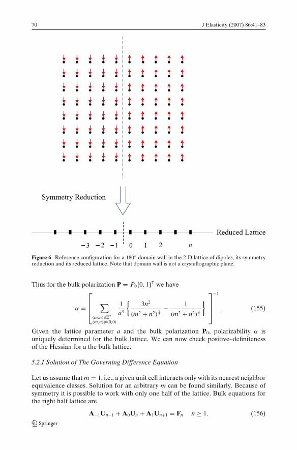
Figure 6 Reference configuration for a 180◦ domain wall in the 2-D lattice of dipoles, its symmetryreduction and its reduced lattice. Note that domain wall is not a crystallographic plane.
Thus for the bulk polarization P = P0{0, 1}T we have
α =
⎡
⎢⎢⎣
∑
(m,n)∈Z2
(m,n) �=(0,0)
1
a3
{3n2
(m2 + n2)52
− 1
(m2 + n2)32
}⎤
⎥⎥⎦
−1
. (155)
Given the lattice parameter a and the bulk polarization P0, polarizability α isuniquely determined for the bulk lattice. We can now check positive–definitenessof the Hessian for a the bulk lattice.
5.2.1 Solution of The Governing Difference Equation
Let us assume that m = 1, i.e., a given unit cell interacts only with its nearest neighborequivalence classes. Solution for an arbitrary m can be found similarly. Because ofsymmetry it is possible to work with only one half of the lattice. Bulk equations forthe right half lattice are
A−1Un−1 + A0Un + A1Un+1 = Fn n ≥ 1. (156)

J Elasticity (2007) 86:41–83 71
Governing equations for n = 0 are boundary equations. These can be written as (notethat U−1 = −U0)
(Ab
0 − Ab−1
)U0 + Ab
1 U1 = F0, (157)
where the superscript b is to emphasize that the boundary stiffness matrices are ingeneral different from the bulk ones. Let us define the following variable
Xn =(
Un−1
Un
)n ≥ 1. (158)
Now the governing equation for Xn is
Xn+1 = AXn + Gn n ≥ 1, (159)
where
A =(
0 1−A−1
1 A−1 −A−11 A0
)∈ R
8×8, Gn =(
0A−1
1 Fn
)∈ R
8. (160)
Note that because of symmetry
Un = −U−n−1 n ≤ −1, (161)
Assuming that Fn = 0 for n > M we have
X2 = Ac + G1,
X3 = A2c + AG1 + G2,
...
XM+1 = AMc + AM−1G1 + ... + GM = AMc + d,
XM+2 = A(AMc + d
),
...
Xn = An−(M+2)(AMc + d
)n ≥ M + 1, (162)
where c = X1 = {U0, U1}T and d = AM−1G1 + ... + GM. For the potential we use itturns out that M = 5 (see Figure 7).
A physically meaningful solution should be bounded at infinity. The matrix Ais not diagonalizable because of translation invariance of the governing equations.9
However, it has the following Jordan decomposition
A = X�X−1, (163)
where X is the matrix of generalized eigenvectors and � has the following form
� =⎛
⎝�1
J�2
⎞
⎠ ∈ R8, �1, �2 ∈ R
2. (164)
9This is the case only for un.

72 J Elasticity (2007) 86:41–83
Figure 7 Unbalanced forces inthe reference configuration ofa 180◦ domain wall in the 2-Dlattice of dipoles. Fx is thecomponent of fx perpendicularto the domain wall and Fp isthe component of fp parallel tothe domain wall. Other forcecomponents are zero becauseof symmetry.
Here �1 and �2 are diagonal matrices of eigenvalues of modulus greater than andsmaller than 1, respectively and J ∈ R
4×4 is the Jordan block corresponding to theeigenvalue λ = 1 with multiplicity four. Now for n ≥ M + 1
Xn = X�n−(M+2)(�MX−1c + X−1d
). (165)
Boundedness equations can be written as
(�MX−1c
){1,...,4} = − (
X−1d){1,...,4} , (166)
where (.){1,...,4} means the first four rows of the matrix (.). Boundary and boundednessequations give us the vector of unknowns c.
The harmonic and anharmonic solution for the numerical values of a = 1.0, P0 =1.0, ε = 1.0
8 , KA = 2.0 are shown in Figure 8. Note that because of symmetry fora given unit cell number n, Un = {ux 0 0 qy}T. Anharmonic lattice statics iterationsconverged after almost 10 iterations. For convergence tolerance for displacement andpolarization unbalanced forces are 10−4 ε
a and 10−4 P0α
, respectively. The harmonic so-lution for the range of interaction m = 2 differs from that of the range of interactionm = 1 by less than 0.5% and the anharmonic displacements are the same. This meansthat the effective potential is highly localized and considering m = 1 is enough.10
However, in each step unbalanced forces are calculated exactly. It is seen that a 180◦domain wall is two lattice spacings thick. Interestingly, this is in qualitative agreementwith our calculations with shell potentials for BaTiO3 and PbTiO3 [42] and also with
10In all the following numerical examples m = 1 is chosen.

J Elasticity (2007) 86:41–83 73
Figure 8 Harmonic andanharmonic displacements in180◦ domain wall in the 2-Dlattice of dipoles.
-0.03
-0.02
-0.01
0
0.01
0.02
0.03
-10 -8 -6 -4 -2 0 2 4 6 8 10
Harmonic
Anharmonic
Harmonic
Anharmonic
a
x
xu
xu
yq
yq
ab initio calculations [31]. To understand the effect of different parameters of thepotential on the domain wall structure, we consider the following four systems
S1 : a = 1.0, P0 = 1.0, ε = 10.0
8, KA = 2.0 (167)
S2 : a = 1.0, P0 = 1.0, ε = 1.0
8, KA = 2.0 (168)
S3 : a = 1.0, P0 = 1.0, ε = 1.0
8, KA = 10.0 (169)
S4 : a = 1.0, P0 = 0.5, ε = 1.0
8, KA = 2.0 (170)
Figure 9 Harmonic andanharmonic displacements forfour different choices of theinteratomic potential.
-0.045
-0.035
-0.025
-0.015
-0.005
0.005
0.015
0.025
0.035
0.045
-10 -8 -6 -4 -2 0 2 4 6 8 10
S1,S2,S3,S4,S1,S2,S3,S4,
a
x
xu
xu
xu
xu
yq
yq
yq
yq

74 J Elasticity (2007) 86:41–83
S2 is the system we just discussed. S1 has a short energy 10 times larger than thatof S2 and S3 has an anisotropic energy five times larger than that of S1. S4 has apolarization with half of the magnitude of that of S1. The anharmonic displacementsof these four systems are compared in Figure 9. It is seen that S1 has the smallest ux
displacements and the other three systems have almost the same ux displacements.This shows that the x displacements are controlled by short-range energy and themore dominant the short-range energy the smaller the x displacements. S1 and S2have the same uq and this is not surprising as they have the same polarizations andthe same anisotropic energies. S3, which has the largest anisotropic energy, has thesmallest uq. S4 has the largest uq which means that the smaller the dipole–dipolecontribution the larger the polarization displacements. An important observation isthat all the four systems have the same domain wall thickness. This is not surprisingas a simple dimensional analysis shows that the domain wall thickness is proportionalto lattice spacing a.
Remark In this example, we presented the exact harmonic solutions. One cansolve an approximate harmonic problem by using a homogenized system in termsof the stiffness matrices. In general, stiffness matrices on the left and right sidesof the wall (and also stiffness matrices for the unit cells close to the wall) aredifferent. One can average the stiffness matrices and then use DFT for solving theresulting homogeneous vector-valued difference equation. The harmonic solutions
Figure 10 a A one-parameter family of reference configurations for the 180◦ domain wall. b A two-parameter family of reference configurations for the same 180◦ domain wall.

J Elasticity (2007) 86:41–83 75
are different from the exact solutions but as the unbalanced forces are calculatedexactly both exact and approximate harmonic solutions lead to the same anharmonicsolutions.
5.2.2 Sensitivity of Solutions to the Choice of Reference Configuration:One and Two-parameter Families of Reference Configurations
Now one may wonder what would happen if one starts with a different referenceconfiguration. We studied the effect of choice of reference configuration on the so-lutions by looking at the one and two-parameter families of reference configurationsshown in Figure 10. In Figure 10a, we assume that polarization vectors in the twolayers adjacent to the wall have magnitude KP0. We solved the governing equationsfor different K values (K ∈ [0.25, 1.75]) and did not observe any new equilibriumconfiguration for any of these large perturbations form the original nominal defect.In Figure 10b a two-parameter family of reference configurations is shown. In thiscase, polarization vectors in the two layers adjacent to the wall have magnitudesK1 P0 or K2 P0. To be able to reduce the governing partial difference equations toan ordinary difference equation one needs to choose a larger unit cell as shown
Figure 11 Referenceconfiguration for a 180◦domain wall in the 2-D latticeof dipoles, its symmetryreduction and its reducedlattice. In this example domainwall passes through someatoms, i.e., it is acrystallographic line.

76 J Elasticity (2007) 86:41–83
in the figure. Again for any choice of K1, K2 ∈ [0.25, 1.75], we obtained the sameequilibrium configuration for the domain wall.
5.3 Example 2: A Second Type of 180◦ Domain Wall
The reference configuration for this type of 180◦ domain wall is shown in Figure 11.In this case lattice vectors are e1 = { a√
2,− a√
2}T and e2 = { a√
2, a√
2}T with polarization
vectors P = P0{0, 1}T. In the bulk, again because of symmetry fx = 0 and one canshow that
α =
⎡
⎢⎢⎣
1
a3
∑
(m,n)∈Z2
(m,n) �=(0,0)
{3(m − n)2
2(m2 + n2)52
− 1
(m2 + n2)32
}⎤
⎥⎥⎦
−1
. (171)
The form of governing equations are exactly similar to the previous example andagain because of symmetry we can reduce the problem to a half lattice. In this
Figure 12 Harmonic andanharmonic displacements in180◦ domain wall in the 2-Dlattice of dipoles.

J Elasticity (2007) 86:41–83 77
example equivalence classes are lines of atoms parallel to the domain wall and a√2
apart from one another. Unbalanced forces are again highly localized. Figure 12shows the harmonic and anharmonic solutions for both position vectors and po-larization for the numerical values of a = 1.0, P0 = 0.5, ε = 1.0, KA = 2.0. Again,displacements are perpendicular to the domain wall and polarization displacementsare parallel to the wall, i.e., for unit cell number n, Un = {ux 0 0 qy}T. It is seen thatthe first harmonic solution is dramatically different from the next iterations and theanharmonic solutions. This is, in general, not surprising and shows the inadequacy ofharmonic solutions for a chosen reference configuration.
5.4 Example 3: A 90◦ Domain Wall in a 2-D Lattice of Dipoles
In this example a 90◦ domain wall is considered. The reference configuration is shownin Figure 13. Governing equations have a form similar to that of 180◦ domain walls.Symmetry of the domain wall implies that polarization force is nonzero only parallelto the domain wall, i.e., because of symmetry for the nth unit cell Un = {ux uy 0 qy}T.We also have the following symmetry
U−n = RU−n−1, R =
⎛
⎜⎜⎝
−1 0 0 00 1 0 00 0 1 00 0 0 −1
⎞
⎟⎟⎠ n ≥ 1. (172)
Figure 13 Referenceconfiguration for a 90◦ domainwall in the 2-D lattice ofdipoles, its symmetryreduction and its reducedlattice. Note that domain wallis not a crystallographic line.
78 J Elasticity (2007) 86:41–83
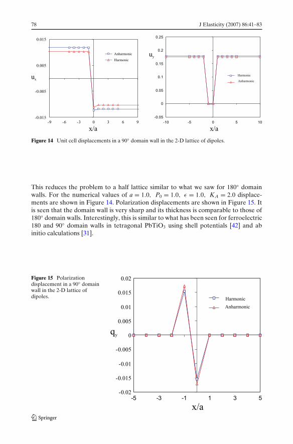
Figure 14 Unit cell displacements in a 90◦ domain wall in the 2-D lattice of dipoles.
This reduces the problem to a half lattice similar to what we saw for 180◦ domainwalls. For the numerical values of a = 1.0, P0 = 1.0, ε = 1.0, KA = 2.0 displace-ments are shown in Figure 14. Polarization displacements are shown in Figure 15. Itis seen that the domain wall is very sharp and its thickness is comparable to those of180◦ domain walls. Interestingly, this is similar to what has been seen for ferroelectric180 and 90◦ domain walls in tetragonal PbTiO3 using shell potentials [42] and abinitio calculations [31].
Figure 15 Polarizationdisplacement in a 90◦ domainwall in the 2-D lattice ofdipoles.

J Elasticity (2007) 86:41–83 79
6 Conclusions
In this paper we developed a general theory of anharmonic lattice statics that canbe used in systematic analysis of a defective crystal given an interatomic potential.This differs from all the existing treatments in that it does not apply only to Bravaislattices and does not rely on a knowledge of force constants. Instead, it can be usedfor arbitrary defective lattices and all is needed is an interatomic potential describingthe interaction of atoms. We started by looking at deformation of a crystal from agiven reference configuration as a discrete deformation mapping and presented allthe developments in a language very similar to continuum mechanics.
We explained how one should construct the discrete governing equations for agiven complex lattice. The discrete governing equations are linearized about a refer-ence configuration. The reference configuration is arbitrary and problem dependentand in general not force-free and perhaps not translation invariant. Our experienceshows that a nominal defect structure could be a good reference configuration. Lin-earizing the (nonlinear) discrete governing equations about the reference configura-tion leads to a nonhomogeneous system of linear difference equations with variablecoefficient matrices. The forcing terms are a result of the fact that the referenceconfiguration is not a local minimum of the energy, in general. We call these forcesthe unbalanced forces. We classified defective complex lattices into three groups,namely defective crystals with 1-D, 2-D and no symmetry reductions. Exploiting asymmetry reduces the dimensionality of the discrete governing equations and thisleads to numerically more efficient solution techniques. Having analytic solutions forlinearized governing equations, the anharmonic solution can be obtained by modifiedNewton–Raphson iterations. The idea is to keep the initial stiffness matrices andupdate the reference configuration by calculating the unbalanced forces in each step.We explained the convergence issue for long range interactions and our presentationis not just formal.
For solving the harmonic displacements we used methods from theory of differ-ence equations. Our solution technique for an infinite defective crystal with a 1-Dsymmetry reduction is novel. For more complicated defective crystals with 2-D andno symmetry reductions we use discrete Fourier transform (DFT) for solving thegoverning partial difference equations. We explained the subtleties in using DFT fortranslation-invariant difference equations.
As an example of a non-isotropic pairwise potential in which atom position vectorsare not the only degrees of freedom, we considered a lattice of point dipoles. Dipole–dipole interactions are pairwise but anisotropic as the potential energy of two dipolesdepends on the dot product of the relative position vector and the polarizationvectors in addition to the relative distance of the two dipoles. It was shown that ourgeneral formulation of lattice statics can easily handle such a system. We were ableto solve two types of 180◦ domain wall problems. It was observed that the domainwall thickness is about two lattice spacings. Interestingly, this is in quantitativeagreement with our calculations with shell potentials for the ferroelectric tetragonalPbTiO3 and also ab initio calculations. In one domain wall problem, it was observedthat harmonic and anharmonic solutions are dramatically different. This shows theimportance of anharmonic effects close to defects. We also solved a 90◦ domainwall problem. It was observed that domain wall thickness is again about two latticespacings. This is again similar to what has been observed for ferroelectric domainwalls in PbTiO3 using shell potentials and ab initio calculations.

80 J Elasticity (2007) 86:41–83
We believe this method can be useful in generating semi-analytical solutions formany different systems with defects. The semi-analytical solutions can be very usefulfor validating numerical techniques. Semi-analytical solutions can also be usefulin studying different interatomic potentials. We believe this development is a stepforward in rationalizing lattice scale calculations.
Acknowledgements The financial support of the Army Research Office under MURI grantNo.DAAD19-01-1-0517 is gratefully acknowledged. We benefited from a discussion on polarizationcatastrophe with Professor P.B. Allen.
Appendix: Three-body Interactions
In this appendix we consider three-body interactions and discuss some of themodifications that should be made in the theory that we developed in the bulk of thispaper. As the effect of pairwise interactions can be studied separately, let us assumethat a collection of atomsL is governed by only three-body interactions. Generalizingthe results of this appendix to arbitrary N-body interactions is straightforward. Theenergy of the system can be written as
E = 1
6
∑
i, j,k∈L( j,k) �=(i,i)
φ(xi, x j, xk). (173)
Note that φ is invariant under permutations of i, j, k. For example, φ(xk, x j, xi) =φ(xi, x j, xk). Because of material-frame-indifference φ has the following dependenceon the position vectors [24]
φ(xi, x j, xk) = ψ(rij, r jk, rki, ωijk, ω jik, ωkij) , (174)
where
r pq = |xp − xq|, ωpqs = (xp − xq) · (xp − xs). (175)
Force on an atom i comes from interactions of i with paris of atoms j, k. Contributionof the triplet (i, j, k) to this force is
fi(i, j, k) = −∂φ(xi, x j, xk)
∂xi. (176)
f j(i, j, k) and fk(i, j, k) are defined similarly. It is an easy exercise to show that
fi(i, j, k) + f j(i, j, k) + fk(i, j, k) = 0. (177)
This is the analogue of the relation f ji = −fij for pairwise interactions. It is easy toshow that balance of angular momentum is trivially satisfied provided that balanceof linear momentum is already satisfied.
Neighboring set Si of atom i ∈ L is the set of all the atoms that interact with i.By definition, i /∈ Si. Neighboring set Sij of the pair of atoms (i, j), i �= j is the setof atoms in L that interact with the pair (i, j). By definition, i, j /∈ Sij. Note also thatSij = Si \ { j}.
Atom energy E i can be defined as one sixth of the energy of all the triplets ofatoms adjacent to i. Pair-atom energy E ij is one half of the energy of all the triplets

J Elasticity (2007) 86:41–83 81
of atoms adjacent to the pair (i, j). Note that energy of the triplet (i, j, k) is triviallydefined as
E ijk = φ(xi, x j, xk). (178)
Let us consider a discrete system of atoms without any external body forces.Linearization of the governing equations about a reference configuration B0 can beexpressed as
∂2E i
∂xi∂xi(B0) ui +
∑
j∈Si
∂2E i
∂x j∂xi(B0) u j = −∂E i
∂xi(B0) . (179)
This can be simplified to read
∂2E i
∂xi∂xi(B0) ui +
∑
j∈Si
∑
k∈Sij
∂2φ(xi, x j, xk)
∂x j∂xi(B0) u j = −∂E i
∂xi(B0) . (180)
Now suppose the defective crystal has a 1-D symmetry reduction, i.e.,
Si =∞⊔
α=−∞
N⊔
I=1
SIα(i). (181)
Thus
∑
j∈Si
∂2E i
∂x j∂xi(B0) u j =
∞∑
α=−∞′
N∑
I=1
∑
j∈SIα(i)
∑
k∈Sij
∂2φ(xi, x j, xk)
∂x j∂xi(B0) uIα
=∞∑
α=−∞′
N∑
I=1
KiIαuIα, (182)
where
KiIα =∑
j∈SIα(i)
∑
k∈Sij
∂2φ(xi, x j, xk)
∂x j∂xi(B0) . (183)
For three-body interactions the following relation holds (as a consequence of trans-lation invariance)
∂2E i
∂xi∂xi= −
∑
j∈Si
∂2E i
∂x j∂xi. (184)
This means that for a defective crystals with 1-D and 2-D symmetry reductions,respectively, we have
KI I0 = −∞∑
α=−∞′
N∑
J=1J �=I
KI Jα, (185)
KI I0 = −∞∑
α,β=−∞′
N∑
J=1J �=I
KI Jαβ, (186)

82 J Elasticity (2007) 86:41–83
which is exactly what we had for pairwise interactions. This is not surprising as theabove relations are a consequence of translation invariance of the lattice irrespectiveof the form of interactions. In conclusion, it is seen that in our formulation of latticestatics, the only modification needed for three-body interactions is in the definitionof substiffness matrices.
References
1. Agarwal, R.P.: Difference Equations and Inequalities. Marcel Dekker, New York (2000)2. Babuska, I.: The Fourier transform in the theory of difference equations and its applications.
Arch. Mech. Stosow. 11(4), 349–381 (1959)3. Babuska, I., Vitásek, E., Kroupa, F.: Some applications of the discrete Fourier transform to
problems of crystal lattice deformation, I,II. Czechoslov. J. Phys. B 10, 419–427, 488–504 (1960)4. Benedetto, J.J.: Harmonic Analysis and Applications. CRC, Boca Raton, Florida (1997)5. Born, M., Huang, K.: Dynamical Theory of Crystal Lattices. Oxford University Press, London,
UK (1988)6. Boyer, L.L., Hardy, J.R.: Lattice statics applied to screw dislocations in cubic metals. Philos. Mag.
24, 647–671 (1971)7. Briggs, W.L., Hendon, V.E.: The DFT: An Owner’s Manual for the Discrete Fourier Transform.
SIAM, Philadelphia, Pennsylvania (1995)8. Bullough, R., Tewary, V.K.: Lattice theory of dislocations. In: Nabarro, F.R.N. (ed.) Dislocations
in Solids, vol. 2. North Holland, Amsterdam, The Netherlands (1979)9. De Boor, C., Holling, K., Riemenschneider, S.: Fundamental solutions of multivariate difference
equations. J. Am. Math. Soc. 111, 403–415 (1989)10. Dennis, J.E., Schnabel, R.B.: Numerical Methods for Unconstrained Optimization and Nonlinear
Equations. SIAM, Philadelphia, Pennsylvania (1996)11. Elaydi, S.N.: An Introduction to Difference Equations. Springer, Berlin Heidelberg New York
(1996)12. Esterling, D.M.: Modified lattice-statics approach to dislocation calculations I. Formalism. J.
Appl. Phys. 49(7), 3954–3959 (1978)13. Esterling, D.M., Moriarty, J.A.: Modified lattice-statics approach to dislocation calculations II.
Application. J. Appl. Phys. 49(7), 3960–3966 (1978)14. Faux, I.D.: The polarization catastrophe in defect calculations in ionic crystals. J. Phys. C, Solid
State Phys. 4, L211–L216 (1971)15. Flocken, J.W.: Modified lattice-statics approach to point defect calculations. Phys. Rev. B 6(4),
1176–1181 (1972)16. Flocken, J.W.: Modified lattice-statics approach to surface calculations in a monatomic lattice.
Phys. Rev. B 15, 4132–4135 (1977)17. Flocken, J.W., Hardy, J.R.: Application of the method of lattice statics to interstitial Cu atoms in
Cu. Phys. Rev. 175(3), 919–927 (1968)18. Flocken, J.W., Hardy, J.R.: Application of the method of lattice statics to vacancies in Na, K, Rb,
and Cs. Phys. Rev. 117(3), 1054–1062 (1969)19. Flocken, J.W., Hardy, J.R.: The method of lattice statics. In: Eyring, H., Henderson, D., (eds.)
Fundamental Aspects of Dislocation Theory, vol. 1 of J.A. Simmons and R. de Wit andR. Bullough, pp. 219–245 (1970)
20. Gallego, R., Ortiz, M.: A harmonic/anharmonic energy partition method for lattice staticscomputations. Model. Simul. Mater. Sci. Eng. 1, 417–436 (1993)
21. Gregor, J.: The Cauchy problem for partial difference equations. Acta Appl. Math. 53, 247–263(1998)
22. Hsieh, C., Thomson, J.: Lattice theory of fracture and crack creep. J. Appl. Phys. 44, 2051–2063(1973)
23. Kanazaki, H.: Point defects in face-centered cubic lattice-I distortion around defects. J. Phys.Chem. Solids 2, 24–36 (1957)
24. Keating, P.N.: Effect of invariance requirements on the elastic strain energy of crystals withapplication to the diamond structure. Phys. Rev. 145(2), 637–645 (1966)
25. King, K.C., Mura, T.: The eigenstrain method for small defects in a lattice. J. Phys. Chem. Solids52(8), 1019–1030 (1991)

J Elasticity (2007) 86:41–83 83
26. Lakshmikantham, V., Trigiante, D.: Theory of Difference Equations: Numerical Methods andApplications. Academic, New York (1988)
27. Lynch, R.E., Rice, J.R., Thomas, D.H.: Direct solution of partial difference equations by tensorproduct methods. Numer. Math. 6, 185–199 (1964)
28. Maradudin, A.A.: Screw dislocations and discrete elastic theory. J. Phys. Chem. Solids 9, 1–20(1958)
29. Maradudin, A.A., Montroll, E.W., Weiss, G.H.: Theory of Lattice Dynamics in The HarmonicApproximation. Academic, New York (1971)
30. Matsubara, T.J.: Theory of diffuse scattering of x-rays by local lattice distortions. J. Phys. Soc.Japan 7, 270–274 (1952)
31. Meyer, B., Vanderbilt, D.: Ab initio study of ferroelectric domain walls in PbTiO3. Phys. Rev. B65, 1–11 (2001)
32. Mickens, R.E.: Difference Equations: Theory and Applications. Chapman & Hall, London, UK(1990)
33. Mura, T.: Micromechanics of Defects in Solids. Martinus Nijhoff, Boston, Massachussetts (1982)34. Ortiz, M., Phillips, R.: Nanomechanics of defects in solids. Adv. Appl. Mech. 59(1), 1217–1233
(1999)35. Shenoy, V.B., Ortiz, M., Phillips, R.: The atomistic structure and energy of nascent dislocation
loops. Model. Simul. Mater. Sci. Eng. 7, 603–619 (1999)36. Tewary, V.K.: Green-function method for lattice statics. Adv. Phys. 22, 757–810 (1973)37. Tewary, V.K.: Lattice-statics model for edge dislocations in crystals. Philos. Mag. A 80(6),
1445–1452 (2000)38. Thomson, R., Zhou, S.J., Carlsson, A.E., Tewary, V.K.: Lattice imperfections studied by use of
lattice Green’s functions. Phys. Rev., B 46(17), 613–622 (1992)39. Tosi, M.P., Doyama, M.: Ion-model theory of polar molecules. Phys. Rev. 160(3), 716–718 (1967)40. Veit, J.: Fundamental solutions of partial difference equations. ZAMM 83(1), 51–59 (2003)41. Vitásek, E.: The n-dimensional fourier transform in the theory of difference equations. Arch.
Mech. Stosow. 12(2), 185–202, 488–504 (1959)42. Yavari, A.: Atomic structure of ferroelectric domain walls, free surfaces and steps. PhD thesis,
California Institute of Technology (2004)