a theory of disagreement in repeated games with …econdm/resources/millerwatson-disagree… · ory...
TRANSCRIPT
http://www.econometricsociety.org/
Econometrica, Vol. 81, No. 6 (November, 2013), 2303–2350
A THEORY OF DISAGREEMENT IN REPEATEDGAMES WITH BARGAINING
DAVID A. MILLERUniversity of Michigan, Ann Arbor, MI 48109, U.S.A.
JOEL WATSONUniversity of California, San Diego, La Jolla, CA 92093-0508, U.S.A.
The copyright to this Article is held by the Econometric Society. It may be downloaded,printed and reproduced only for educational or research purposes, including use in coursepacks. No downloading or copying may be done for any commercial purpose without theexplicit permission of the Econometric Society. For such commercial purposes contactthe Office of the Econometric Society (contact information may be found at the websitehttp://www.econometricsociety.org or in the back cover of Econometrica). This statement mustbe included on all copies of this Article that are made available electronically or in any otherformat.
Econometrica, Vol. 81, No. 6 (November, 2013), 2303–2350
A THEORY OF DISAGREEMENT IN REPEATEDGAMES WITH BARGAINING
BY DAVID A. MILLER AND JOEL WATSON1
This paper proposes a new approach to equilibrium selection in repeated gameswith transfers, supposing that in each period the players bargain over how to play. Al-though the bargaining phase is cheap talk (following a generalized alternating-offerprotocol), sharp predictions arise from three axioms. Two axioms allow the players tomeaningfully discuss whether to deviate from their plan; the third embodies a “the-ory of disagreement”—that play under disagreement should not vary with the man-ner in which bargaining broke down. Equilibria that satisfy these axioms exist for alldiscount factors and are simple to construct; all equilibria generate the same welfare.Optimal play under agreement generally requires suboptimal play under disagreement.Whether patient players attain efficiency depends on both the stage game and the bar-gaining protocol. The theory extends naturally to games with imperfect public monitor-ing and heterogeneous discount factors, and yields new insights into classic relationalcontracting questions.
KEYWORDS: Relational contracts, repeated games, self-enforcement, equilibriumselection, bargaining, renegotiation, disagreement.
1. INTRODUCTION
MANY ECONOMIC RELATIONSHIPS (such as partnership, employment, andbuyer-supplier relationships) are ongoing and governed in whole or in partby self-enforcement. The relational contracts literature studies these relation-ships using the framework of infinitely repeated games, but repeated gamessuffer from a vast multitude of equilibria, particularly when players are pa-tient. So equilibrium theory alone offers little hope for predicting behavior orfor identifying parameters from observed behavior.
To understand these ongoing relationships, one needs a theory of equilib-rium selection. Informally, it seems that players in an ongoing relationshipmust coordinate closely so as to select “their” equilibrium from the multitude,
1We thank Nageeb Ali, Jim Andreoni, Sylvain Chassang, Vince Crawford, Marina Halac, MattJackson, Sebastian Kranz, Ola Kvaløy, Jin Li, Garey Ramey, Larry Samuelson, Joel Sobel, andseveral anonymous referees for valuable comments and suggestions, along with seminar partic-ipants at Arizona, Collegio Carlo Alberto, Columbia, Duke-Fuqua, ETH Zurich, Florida Inter-national, IFPR, Johns Hopkins, Microsoft Research, Penn, Santa Fe Institute, Toronto, UCLA,UCSD, UC Davis, USC, USC-Marshall, Washington University, Western Ontario, and Yale, andconference participants at the GTS Third World Congress, SWET 2008, the 2008 Stony BrookWorkshops, the 2009 NBER Organizational Economics Working Group, and NAWMES 2011.Jacob Johnson, Jong-Myun Moon, and Aniela Pietrasz provided excellent research assistance.Miller thanks the NSF (SES-1127643), Microsoft Research, Yale, and the Cowles Foundationfor hospitality and financial support; Partha Dasgupta for inspiration to pursue this topic; andhis former colleagues at UCSD for all their support. Watson thanks the NSF (SES-0095207 andSES-1227527), the NOAA Fisheries Service, Yale, the Cowles Foundation, and the Center forAdvanced Study in the Behavioral Sciences at Stanford for hospitality and financial support.
© 2013 The Econometric Society DOI: 10.3982/ECTA10361

2304 D. A. MILLER AND J. WATSON
so it often makes sense to suppose that they coordinate on a Pareto-optimalequilibrium. But this intuition raises two issues. First, payoffs on the Paretofrontier may be supported by the threat of punishments that depart from thePareto frontier. What if the players can re-coordinate their continuation playto escape from a Pareto-dominated punishment? Second, there are typicallymany equilibria on the Pareto frontier, where one player’s gain is necessarilya loss for others. How do they decide which Pareto-optimal equilibrium to se-lect? Though these issues have arisen in the relational contracts literature, aunified solution is lacking.2
We resolve these issues by modeling equilibrium selection as a noncoop-erative bargaining process embedded in a repeated game with transfers. Ineach period, the players engage in cheap-talk bargaining via a generalizedalternating-offer protocol and make voluntary transfers prior to playing thestage game. We propose three axioms that endow cheap-talk messages withendogenous meaning. Any equilibrium that satisfies these axioms—which wecall a contractual equilibrium—has a simple representation. In a contractualequilibrium, the bargaining protocol influences both the welfare level (the sumof the players’ payoffs) and the distribution of welfare. These implications havea simple interpretation in terms of relative bargaining power.
We provide an explicit algorithm for constructing contractual equilibria, andwe characterize their efficiency and allocative properties. We also extend thetheory to games with more than two players, imperfect public monitoring, andheterogeneous discount factors. To demonstrate the utility of contractual equi-librium for the study of relational contracts, we show how the theory generatesnew insights in two principal-agent applications. We discuss how our theory re-lates to findings in the empirical macro labor literature and the experimentalliterature on preplay communication, bargaining, and repeated games. In par-ticular, our results suggest that it may be fruitful for both literatures to explorethe role of bargaining power in more depth.
Axioms on Endogenous Meaning
Section 3 describes our axioms and Section 4 gives them a dynamic program-ming representation. The first axiom, Internal Agreement Consistency (IAC),ensures that a class of “agreements” has meaning. Specifically, if a player pro-poses playing as if to switch to a different history in the same equilibrium andif this offer is accepted, then the players play as agreed. By itself, IAC doesnot change the set of equilibrium payoffs in the game (Theorem 1). A de-viant agreement to switch histories can always be discouraged by punishing theplayer who proposes it and rewarding the one who rejects it.
2There is also the renegotiation-proofness literature, which addresses the first issue, but gen-erally not the second. We discuss renegotiation proofness later in this section and in more depthin Section 8.
DISAGREEMENT IN REPEATED GAMES 2305
The second axiom, No-Fault Disagreement (NFD), embodies a theory of dis-agreement. It specifies that if the players do not reach agreement in a given pe-riod, then their continuation play should not depend on how bargaining brokedown. The idea is that no player should be selectively punished for putting aninnovative offer on the table or for rejecting the equilibrium offer in hopes ofbeing able to make an innovative counteroffer. Disagreement also implies zeromonetary transfers in the current period, which is equivalent to saying thatfailure to make an agreed-upon transfer induces disagreement. NFD allowscontinuation play under disagreement to be Pareto dominated by continuationplay under agreement, and it may vary with the past history of actions. By it-self, NFD has little influence over the set of equilibrium payoffs in the game(Theorem 2).
Putting IAC and NFD together, however, leads to a significant refinementwith a simple representation (Theorem 3(i)). For any given history, the bar-gaining phase has a well-defined disagreement value and, in equilibrium, theplayers divide the surplus according to the allocation of bargaining power thatarises from the bargaining protocol. Across periods, agreement and disagree-ment values are linked by enforceability conditions along the lines of Abreu,Pearce, and Stacchetti (1990). The set of equilibrium payoffs available underIAC and NFD is typically much smaller than the set of all subgame-perfectequilibrium payoffs. For instance, in some prisoners’ dilemma games, the onlypossible outcome is infinite repetition of the stage-game equilibrium, regard-less of how patient the players are (see Section 5.4).
Generally, there may be multiple, Pareto-ranked payoff sets available un-der IAC and NFD. The third axiom, Pareto External Agreement Consistency(PEAC), formalizes the intuition that players should be expected to select aPareto-optimal equilibrium. It ensures meaning for any agreement to play as ifswitching to an equilibrium that both fully Pareto dominates the current equilib-rium and also satisfies IAC and NFD. Under IAC, NFD, and PEAC, the play-ers agree to play a fully Pareto-dominant subgame-perfect equilibrium amongthose that satisfy IAC and NFD (Theorem 3(ii)).
Characterization of Contractual Equilibrium
In Section 5, we characterize the set of contractual equilibrium values. The-orem 4 shows that, for any discount factor, this set is a compact line segmentof slope −1. Theorem 5 provides an explicit algorithm for constructing it. Thealgorithm involves computing two optimal disagreement points that pin downthe endpoints, along with an optimal agreement outcome that determines theplayers’ welfare. Theorem 6 provides necessary and sufficient conditions forpatient players to attain efficiency. We show that the allocation of bargainingpower affects welfare and that welfare is maximized by assigning all bargain-ing power to one of the players (Theorem 7). Section 6 generalizes contractualequilibrium to games with more than two players, imperfect public monitoring,
2306 D. A. MILLER AND J. WATSON
and heterogeneous discount factors. Theorem 8 shows that the set of contrac-tual equilibrium values forms a nonempty, compact hyperpolygon.
Foundations for Relational Contracts
The relational contracts literature examines how agreements can be self-enforced in environments with repeated play and limited external enforce-ment. Existing approaches have produced many insights, but mostly skirtaround the question of how agents initiate and manage their relationships.3These assumptions simplify analysis, but leave open the implications of bar-gaining power and how self-enforced agreements evolve after deviations.
Section 7.1 illustrates our approach by applying it to the principal-agentmodel studied by Levin (2003). Levin applied “strong optimality,” a variantof renegotiation proofness that, in this model, implies that the principal can-not make a meaningful deviant offer to the agent, even if she has a monopolyover making proposals. In contrast, in our approach, bargaining power mat-ters: the agent’s effort is increasing in his own bargaining power. Surprisingly,the principal’s ideal level of bargaining power is intermediate: if she has allthe bargaining power, she cannot commit to payments that would motivate theagent; if she has no bargaining power, then the agent extracts all the surplus.
In Section 7.2, we apply contractual equilibrium to the interaction of “ex-plicit” (externally enforced) contracts and “implicit” (self-enforced) contracts,inspired by Baker, Gibbons, and Murphy (1994) and related work by Schmidtand Schnitzer (1995). These papers assume that parties are limited to externalenforcement following any deviation, implying that an improvement in exter-nal enforcement can reduce equilibrium welfare. In contractual equilibrium,the parties can reevaluate their entire relationship whenever they bargain, soequilibrium welfare always weakly increases in the strength of external enforce-ment. In Section 7.3, we discuss how the framework developed here can helpextend macro labor models to combine moral hazard, bargaining power, and
3Most approaches simply select an equilibrium on the Pareto frontier (e.g., Radner (1985),Ramey and Watson (1997, 2001), Pearce and Stacchetti (1998), Levin (2002, 2003), Doornik(2006), Fuchs (2007), Rayo (2007), Chassang (2010)). Some assume that after a deviation, theplayers renegotiate permanently to the optimal spot contract (e.g., Thomas and Worrall (1988),Baker, Gibbons, and Murphy (1994, 2002), Schmidt and Schnitzer (1995), Kvaløy and Olsen(2006, 2009), Hermalin, Li, and Naughton (2013)); Baker, Gibbons, and Murphy (2002) alsoallowed reallocation of ownership rights. Others allowed for renegotiation once the relationshipis underway, but assume that disagreement causes the parties to separate or switch to a stage-game equilibrium permanently (MacLeod and Malcomson (1998), Jackson and Palfrey (1998),Ramey and Watson (2002)). A few employed renegotiation proofness (MacLeod and Malcom-son (1989), Levin (2003)). Even those who allowed for continued interaction following disagree-ment assumed that the players temporarily either receive an exogenous outside option (MacLeodand Malcomson (1989), Levin (2002), Halac (2012), Fong and Li (2010, 2012)) or play an exoge-nously selected stage Nash equilibrium (Raff and Schmidt (2000), Klimenko, Ramey, and Watson(2008)).
DISAGREEMENT IN REPEATED GAMES 2307
continued interaction under disagreement. We also discuss connections withthe empirical literature, where there are suggestive results that link differencesin relative bargaining power to productive outcomes.
Contrast With Renegotiation Proofness
The literature on renegotiation proofness in infinitely repeated games, ini-tiated by Rubinstein (1980), Bernheim and Ray (1989), Farrell and Maskin(1989), and Pearce (1987), addresses the problem of Pareto-dominated contin-uation play by ruling it out. That is, for a given equilibrium, if the continuationfrom any particular history is dominated by a qualified alternative, then theequilibrium is removed from consideration. So unlike contractual equilibrium,renegotiation proofness does not model renegotiation explicitly, so it does notcontemplate the possibility of disagreement. By capturing the effect of bargain-ing power in a tractable way, contractual equilibrium yields substantively dif-ferent testable implications about the players’ welfare than does renegotiationproofness. Section 5.4 illustrates the comparison between these approachesand Section 8 discusses their relationship in more depth.
2. REPEATED GAMES WITH BARGAINING
2.1. Extensive Form
Consider a repeated game augmented with cheap-talk bargaining and trans-ferable utility. Formally, a two-player game in this class is defined by a stagegame 〈A�u〉, a common discount factor δ ∈ (0�1), and a bargaining protocolthat we describe shortly. Here A ≡ A1 × A2 is the space of action profiles andu : A → R
2 is the stage-game payoff function. We normalize the payoffs by1−δ as is standard. Each period comprises four phases: (i) the public random-ization phase, (ii) the bargaining phase, (iii) the transfer phase, and (iv) theaction phase. In the public randomization phase, the players observe an arbi-trary public randomization device.4 In the transfer phase, the players simulta-neously make voluntary, nonnegative monetary transfers; that is, each playerdecides how much money to pay to the other, where money enters their utilityquasilinearly. In the action phase, the players play the stage game 〈A�u〉. Thestage game can also include voluntary transfers that occur simultaneously withother actions. There is no external enforcement of any kind.
In the bargaining phase, the players engage in a generalized alternating-offerbargaining protocol. The number of potential rounds of bargaining may befinite or infinite, but all these rounds occur in a mere instant, so bargainingdoes not delay the later phases of the period. (If bargaining involved delay, it
4Such devices are standard in repeated games analysis (see Fudenberg and Maskin (1986)).Here, the device should be viewed as having been constructed by the players in their process ofequilibrium selection.
2308 D. A. MILLER AND J. WATSON
would not be cheap talk.) There is an exogenous random recognition processρ ∈ (�{1�2})∞ that selects one of the players to make a verbal statement ineach round of bargaining, where ρi�� is the probability that player i is recog-nized in round �. The selected player—called the proposer—selects a proposalfrom some language set L and this is observed by the other player, who iscalled the responder. If the response is “yes,” indicating the responder’s accep-tance, then the bargaining phase ends and the game proceeds to the transferphase. If the response is “no,” then bargaining may either break down or con-tinue to another round. If bargaining breaks down, then play proceeds to thetransfer phase. Breakdown is triggered randomly by a process β ∈ [0�1]∞ with∏∞
�=1(1 − β�) = 0, where β� is the probability that breakdown occurs after a“no” response in bargaining round �. Both the recognition process and thebreakdown process are invariant to the time period and the history; they de-pend only on the round of bargaining within a period.
The language L should be sufficiently large that each player can use it to pro-pose to the other how to coordinate their continuation play.5 Specifically, weassume that L contains the space of possible continuation payoff vectors fromthe voluntary transfer phase, so that a proposal w ∈ R
2 should be interpretedas a suggestion to coordinate on play in the continuation game to achieve w asthe continuation value.
ASSUMPTION 1—Rich Language: It is the case that R2 ⊂ L.
Next we develop some notation for histories. We start by describing out-comes of the bargaining phase within a period. Suppose bargaining lasts �rounds, at which point an offer is accepted or there is exogenous break-down. Such an outcome is fully described by an element of ({1�2} × L)� ×{agreement, breakdown}, where, for each round of bargaining, {1�2} accountsfor the identity of the proposer and L accounts for the proposal. For thefirst � − 1 rounds, the response was “no.” Then, for round �, “agreement”signifies that the last proposal was accepted, whereas “breakdown” signifiesthat bargaining broke down. Thus the set of possible bargaining outcomes isB ≡ ⋃∞
�=1({1�2} × L)� × {agreement, breakdown}.The set of full-period histories, including the “null history,” is H ≡ ⋃∞
t=0(Ω×B × R+ × R+ × A)t , where Ω is the state space of the arbitrary public random-ization device. Here the first R+ accounts for transfers from player 1 to player2, and the second R+ accounts for transfers from player 2 to player 1. The net ofthese transfers is summarized by a transfer vector in R
20 ≡ {m ∈ R
2|m2 = −m1}.
5One might wish to assume that L contains descriptions of all continuation strategy profiles inthe game. However, since such a construction would be circular (strategies would specify history-dependent statements in each negotiation phase, and these statements would include the descrip-tion of an entire strategy profile), it would lead to a difficult technical issue regarding whether anappropriate “universal language” exists.
DISAGREEMENT IN REPEATED GAMES 2309
A history to the transfer phase is an element of H ×Ω× B. A history to the actionphase is an element of H ×Ω× B ×R+ ×R+. A history to the transfer phase orto the action phase is under agreement if the just-completed bargaining phaseended with “agreement”; otherwise the history is under disagreement.
2.2. Recursive Characterization of Equilibrium Values
We characterize the set of subgame-perfect equilibrium (SPE) payoffs by ex-tending the recursive methods of Abreu, Pearce, and Stacchetti (1990), work-ing backward through the phases of a given period. Consider first the actionphase. Let �A be the set of probability distributions over A that are indepen-dent across dimensions, that is, the set of mixed action profiles that can arisefrom independent mixed actions for each player. In equilibrium, the mixedaction profile must constitute a Nash equilibrium, taking the players’ contin-uation play from the following period as given. Formally, if g : A → R
2 givesthe continuation value as a function of the realized action profile a ∈ A and ifα ∈ �A is a Nash equilibrium of 〈A� (1 − δ)u+ δg〉, then g enforces α. In thiscase, the continuation value from the action phase is
w = (1 − δ)u(α)+ δg(α)(1)
If W ⊂ R2 is the set of feasible continuation values starting next period, then
the set of continuation values supported from the action phase of the currentperiod is
D(W ) ≡ {w ∈ R
2∣∣(2)
∃g : A → W and α ∈ �As.t. g enforces α and Eq. (1) holds
}
Define Di(W )≡ ⋃w∈D(W )[wi�∞) and let D(W )≡D1(W )×D2(W ). The set of
continuation values supported from the transfer phase is
C(W ) ≡ {w ∈ R
2∣∣(3)
∃m ∈ R20 and w′ ∈ D(W )
s.t. w = (1 − δ)m+w′ and w ∈D(W )}
To understand how values in C(W ) can be achieved, consider any w, m, andw′ that satisfy the conditions of Eq. (3). Without loss of generality, take thecase of m1 ≥ 0 so that player 2 is supposed to make a transfer to player 1.Prescribe that player 2 make this transfer and then the players continue withbehavior to achieve w′ from the action phase. If player 2 does not make therequired transfer, then the players coordinate on behavior to achieve a value
2310 D. A. MILLER AND J. WATSON
w ∈ D(W ) from the action phase, where w is selected so that w2 ≥ w2. Clearlythe prescribed behavior is rational from the transfer phase.6
Operator C provides the basis for the recursive formulation of SPE payoffs.Given a set of equilibria S, let V (S) be the set of continuation values attainedby S starting from any full-period history. When V is evaluated at a single-ton set {s}, we call it the value set of s and abuse notation to write V (s). LetSSPE be the set of all subgame-perfect equilibria of our model with bargaining.From the construction above, it is clear that V (SSPE) is the largest fixed point ofcoC(·), where co denotes the convex hull to account for public randomizationat the beginning of each period. Also observe that V (SSPE) is identical to theset of subgame-perfect equilibrium payoffs in an otherwise identical game withno bargaining phase, denoted V (SNB).7
3. AXIOMATIZATION OF ENDOGENOUS MEANING
So far, statements in L neither have any particular meaning nor impose anyconstraints on the set of equilibrium payoffs. We next develop axioms that re-fine the equilibrium set by imposing meaning in equilibrium. Our axioms arein the spirit of equilibrium restrictions introduced by the literature on preplaycommunication, as discussed in Section 8.
3.1. A Foundation for Meaningful Proposals
In an equilibrium s ∈ SSPE, the players recognize that any payoff inC(coV (s)) is attainable from the transfer phase by randomizing over con-tinuation values achieved by s using the public randomization device at thebeginning of the next period. We posit that the players should have the oppor-tunity to agree on such a payoff and then follow through on their agreement;that is, any proposal to play as if conditionally switching to different histories inthe same equilibrium should be taken seriously. Our first axiom requires that,on or off the equilibrium path, if there is agreement on a continuation valuew that is consistent with the equilibrium strategy profile (the proposer offersw ∈ C(coV (s)) and the responder says “yes”), then the players proceed in away that achieves value w.
6Nothing more can be supported since feasibility requires w = (1 − δ)m+w′ for some m ∈ R20
and w′ ∈ D(W ), and each player i can guarantee himself some value in Di(W ) by making a zerotransfer. Also note that it is not helpful to have both players make positive transfers—one couldreduce both transfers equally until one equals zero, loosening the incentive constraints withoutaffecting the continuation value. For more details, see Goldlücke and Kranz (2012).
7The players can always ignore the bargaining phase, so V (SSPE) ⊇ V (SNB). Similarly, sinceboth games feature arbitrary public correlation devices and the bargaining phase is pure cheaptalk, V (SSPE)⊆ V (SNB).
DISAGREEMENT IN REPEATED GAMES 2311
AXIOM IAC—Internal Agreement Consistency: For every history to the trans-fer phase under agreement, if the agreement satisfies w ∈C(coV (s)), then contin-uation play yields value w.8
Let SIAC be the subset of SSPE that satisfies IAC. Note that IAC does notrequire the players to reach agreement. It merely defines the meaning of aclass of agreements, refining the equilibrium set due to the consequences inoff-equilibrium-path contingencies. Though IAC eliminates some equilibria, itdoes not on its own refine the equilibrium value set.
THEOREM 1—IAC Has No Bite: It is the case that V (SIAC)= V (SSPE).
The proof, in Appendix A.1, actually strengthens the result by invoking astronger consistency axiom that also addresses agreements to switch to contin-uations that are supported by other equilibria. Under IAC there may be de-viant proposals that, if implemented, would make the proposer better off thanif he made his equilibrium proposal. However, it is always possible to deter adeviant proposal by specifying that if the responder says “no,” then the playersshould coordinate to punish the proposer and reward the responder. In thisway, the agreement consistency axiom is undermined by the fact that continu-ation play can vary in arbitrary ways following a disagreement. To narrow theset of equilibrium values, we need a theory of disagreement.
3.2. A No-Fault Theory of Disagreement
We next add a no-fault disagreement axiom that embodies a theory of howplayers behave under disagreement. It requires that continuation play in theabsence of agreement—though it may vary with the history of actions, trans-fers, and past agreements—should not vary with the manner in which bargain-ing broke down.
Disagreement can arise in myriad ways. Bargaining may randomly breakdown after a responder says “no,” following any sequence of equilibrium ordeviant offers. That disagreement play should not be sensitive to the mannerof breakdown represents the nostrum that “nothing is agreed until everythingis agreed.” That is, no player can be singled out for punishment for making aninnovative, deviant offer that is rejected or for rejecting an offer in hopes ofbeing able to make an innovative counteroffer. We also assume that play fromthe action phase under disagreement is insensitive to the transfers just made so
8For simplicity, we state IAC in a somewhat stronger form than is necessary. The necessary partis that the players should achieve the value of an agreement w if it is attainable with a transfer andany continuation w′ ∈ D(coV (s)) that is actually attained by s after some history to the actionphase.
2312 D. A. MILLER AND J. WATSON
as to capture the idea that a player can void an agreement by refusing to makethe required up-front payment.9
AXIOM NFD—No-Fault Disagreement: For every history to the action phaseunder disagreement, continuation play is measurable with respect to the full-periodhistory at the end of the previous period and the current-period realization of thepublic randomization device.10
Although NFD constrains the meaning of disagreements, by itself NFD doeslittle to constrain the set of attainable payoffs. In particular, in the realm ofpure-strategy equilibria, NFD does not alter the Pareto boundary of equilib-rium continuation values; neither does it eliminate any payoffs attainable in asubgame-perfect equilibrium without transfers.
To state this result, we need to introduce some extra notation; the proofis given in Appendix A.1. Let SNFD be the subset of SSPE that satisfies NFD.Let Sps
SPE be the set of pure-strategy subgame-perfect equilibria, let SpsNFD be the
subset of pure-strategy equilibria that satisfy NFD, and let SntSPE be the set of
subgame-perfect equilibria that specify zero transfers after all histories. Forany set of payoffs W ⊂ R
2, let P(W ) be the Pareto frontier of W .
THEOREM 2—NFD Has Little Bite: It is the case that P(V (SpsSPE)) =
P(V (SpsNFD)) and V (Snt
SPE)⊆ V (SNFD).
In combination with IAC, however, NFD has strong effects. In particular, itrules out the kinds of punishments used to discourage deviant proposals in theproof of Theorem 1. Following any history, the bargaining phase (viewed inisolation as a game in itself) has a unique disagreement outcome by NFD, anda nondegenerate bargaining set by IAC. Therefore, it has unique subgame-perfect equilibrium, as established by the literature on alternating-offer bar-gaining (Binmore (1987), Rubinstein (1982), Shaked and Sutton (1984)). Wecharacterize the implications of NFD and IAC in Section 4.
Although the combination of NFD and IAC eliminates many equilibria, mul-tiple Pareto-ranked equilibrium payoffs generally still survive. Our third axiomallows the players to meaningfully discuss whether to switch to an equilibriumthat is “better” than the one they are currently playing. The following defini-tion formalizes what makes one equilibrium better than another.
9In other words, transfers “seal the deal.” In the realm of relational contracts, where there isalways at least a rudimentary legal system in the background, this interpretation embodies thefact that signing a contract can create a legal obligation to make an unconditioned payment, evenwhen no other contract clauses are legally enforceable. Adopting this interpretation formallywould require extra notation to keep track of the transfer required in agreement. Then, with aslightly different version of IAC, we would obtain the same implications.
10Again, for simplicity, we state the axiom in a simpler, stronger form than needed. Section 8.1discusses how NFD could be weakened without affecting the results.
DISAGREEMENT IN REPEATED GAMES 2313
DEFINITION 1: A payoff set W ′ ⊂ R2 fully Pareto dominates another payoff
set W if (i) for every v′ ∈ W ′, there is no v ∈ W \W ′ that satisfies v ≥ v′ (com-ponentwise), and (ii) for every v ∈ W , there exists v′ ∈ W ′ such that v′ ≥ v(componentwise).
We say that a strategy profile s′ fully Pareto dominates another strategy profiles if coV (s′) fully Pareto dominates coV (s). Because full Pareto dominance isa demanding notion of dominance, the following axiom—that the players musthonor any agreement to deviate to an equilibrium that fully Pareto dominatestheir current equilibrium—is relatively weak.
AXIOM PEAC—Pareto External Agreement Consistency: For every historyto the action phase under agreement in equilibrium s, if the agreement satisfies w ∈C(coV (s′)), where s′ ∈ SIAC ∩ SNFD and coV (s′) fully Pareto dominates coV (s),then continuation play yields value w.
As with IAC, Appendix A.1 shows that PEAC has no bite.
COROLLARY 1—PEAC Has No Bite: We have V (SPEAC)= V (SSPE).
But the three axioms together yield a sharp characterization. We define acontractual equilibrium to be any subgame-perfect equilibrium that satisfiesIAC, NFD, and PEAC. Accordingly, let SPEAC be the set of equilibria that sat-isfy PEAC and let SCE ≡ SIAC ∩ SNFD ∩ SPEAC. The next section shows thatV (SCE) is identical to a “dominant bargaining self-generated set” that we iden-tify. The rest of this paper is devoted to characterizing this set.
4. REPRESENTATION
To characterize contractual equilibrium values, we compare the bargainingphase in an individual period to a simple bargaining game in which (i) the play-ers bargain directly over a fixed set of payoff vectors and (ii) the generalizedalternating-offer protocol is of the form described in Section 2.1. Analysis ofthis simple bargaining game yields a “bargaining operator” that we embed in arecursive construction of continuation values.
In the simple bargaining game, the players bargain over the selection of apayoff vector from a set W ⊂ R
2. If they fail to reach an agreement, then thepayoff vector is some value w ∈ W . Suppose that the sum of the players’ con-tinuation payoffs—which we call the welfare level—is constant along the Paretoboundary of W , and suppose this boundary includes all points above w with thesame welfare. Then the unique subgame-perfect equilibrium payoff vector wsatisfies
w1 +w2 = maxw′∈W
(w′
1 +w′2
)and w = w+π(w1 +w2 −w1 −w2)�(4)
2314 D. A. MILLER AND J. WATSON
where for each player i, πi = ∑∞�=1(ρi��β�
∏�−1k=1(1 − βk)). In other words, the
players maximize welfare, and they split the surplus in fractions π1 and π2. Thisconclusion is stated in Lemma 6 in Appendix A.2. Let π = (π1�π2) and notethat π1 +π2 = 1.
Next we construct a set of payoff vectors by calculating the equilibrium pay-offs that can arise in the simple bargaining game when w can be any disagree-ment value in W :
B(W �W )≡{w +π
(maxw∈W
(w1 +w2)−w1 −w2
) ∣∣∣w ∈ W}(5)
Returning to the repeated game, recall that operators D and C produce thesets of continuation values from the action phase and transfer phase of a givenperiod, respectively, as a function of a set of continuation values W from thestart of the following period. We interpret C(W ) as the set of payoff-vectoralternatives for the players in the bargaining phase and interpret D(W ) as theset of disagreement payoffs attainable from the transfer phase (with transfersof zero). The bargaining operator, along with public randomization at the be-ginning of the period, yields the compound operator coB(C(·)�D(·)).11 Weexamine fixed points of this compound operator.
DEFINITION 2: A nonempty set W ⊂ R2 is called a bargaining self-generated
(BSG) set if W = coB(C(W )�D(W )).
Our next definition combines bargaining self-generation with full Paretodominance.
DEFINITION 3: A BSG set W ∗ ⊂ R2 is dominant if it fully Pareto dominates
every other BSG set.
By definition, there can be at most one dominant BSG set. Our represen-tation theorem establishes a relation between sets of contractual equilibriumvalues and bargaining self-generated sets. The theorem shows that the valueset of every contractual equilibrium is contained in the dominant BSG set, andfor each value in the dominant BSG set, there is a contractual equilibrium thatdelivers it.
THEOREM 3—Representation: Given a game 〈A�u�δ�ρ�β〉, let πi =∑∞�=1(ρi��β�
∏�−1k=1(1 −βk)) for each i. Then the following properties hold:
(i) If W is a BSG set, then W ⊆ V (SIAC ∩ SNFD); furthermore, if s ∈ SIAC ∩SNFD, then coV (s) is a BSG set.
(ii) The set V (SCE) is the dominant BSG set.
11Recall that D(W ) ⊂ C(W ), welfare is constant along the Pareto boundary of C(W ), andC(W ) extends to the edges of D(W ) along each player’s axis. This implies that B(C(·)�D(·)) iswell-defined.
DISAGREEMENT IN REPEATED GAMES 2315
The proof is given in Appendix A.2. In principle, every point in V (SCE) is anequally good candidate to be selected as the equilibrium payoff in the first pe-riod. By construction, the first period payoff must be v = B(C(V (SCE))� {w}),where w ∈ D(V (SCE)) is the payoff that arises if the players disagree in the firstperiod. But nothing pins down which point in D(V (SCE)) is selected to be thedisagreement point in the first period—neither the axioms nor any prior agree-ment. The same is true of the disagreement payoff in any period following ahistory in which the players have never agreed. So the problem of selectinga particular equilibrium boils down to determining how the players will play ifthey have never agreed. In applications, this behavior might arise from custom,the status quo, or social institutions.
Note that the bargaining-protocol parameters ρ and β enter the definitionof the compound operator coB(C(·)�D(·)) in ways summarized by π1 and π2.Thus, the recursive construction of contractual equilibrium values can use asimplified description of the game, given by 〈A�u�δ�π〉. Also, the standardconnection between the subgame-perfect equilibrium of the noncooperativebargaining game and a cooperative bargaining solution applies here. In partic-ular, the equilibrium payoff w shown in Eq. (4) coincides with the generalizedNash (1950) bargaining solution with weights π1 and π2. Thus, we call π avector of “bargaining weights,” understanding that these weights represent thebargaining protocol.
5. CHARACTERIZATION
This section characterizes the set of contractual equilibrium values V (SCE)and provides an algorithm for computing it. This section also provides resultson efficiency and how bargaining power affects what values are attainable. Thecharacterization shows that every BSG set (and hence V (SCE)) is a line seg-ment with slope −1. Equivalently, every BSG set has two endpoints z1� z2 ∈ R,satisfying z1
1 + z12 = z2
1 + z22 . Let z1 be the endpoint that favors player 2 (“pun-
ishing” player 1) and let z2 be the endpoint that favors player 1. For any suchset W , we define span(W )≡ z2
1 −z11 = z1
2 −z22 and level(W )≡ z1
1 +z12 = z2
1 +z22 ,
which are the vertical distance, or payoff span, across W and the joint value, orwelfare level, respectively, of each point in W .
5.1. Existence and Construction
We begin by showing that V (SCE) exists for any discount factor.
THEOREM 4—Existence: For a game 〈A�u�δ�π〉, if A is finite, then V (SCE)is a nonempty, compact line segment of slope −1.
The next result provides a complete, constructive characterization of V (SCE).
2316 D. A. MILLER AND J. WATSON
THEOREM 5—Construction: For a game 〈A�u�δ�π〉, if A is finite and W ∗ =V (SCE), then the following properties hold:
(i) The span(W ∗) is equal to the maximal fixed point of Γ ≡ γ2 + γ1, wherefor players i �= j,
γj(d)≡ maxη�α
(πjui(α)−πiuj(α)+ δ
1 − δη(α)
)(6)
s.t.
⎧⎨⎩η : A → [−d�0]� extended to �Aα ∈ �A is a Nash equilibrium
of⟨
Ai × Aj� (1 − δ)(ui�uj)+ δ(η�−η)⟩
(ii) level(W ∗) is equal to maxη�α(u1(α)+ u2(α))
s.t.
{η : A → [
0� span(W ∗)]� extended to �A
α ∈ �A is a Nash equilibrium of⟨
A� (1 − δ)u+ δ(η�−η)⟩
(7)
(iii) The endpoints of W ∗ are
z1 = (−1�1)γ1(span
(W ∗)) +π level
(W ∗)�(8)
z2 = (1�−1)γ2(span
(W ∗)) +π level
(W ∗)(9)
The rest of this subsection contains the proof of Theorems 4 and 5. We pro-ceed with a series of lemmas that characterize the geometry of BSG sets andthe relation between them; we then identify a dominant BSG set. Proofs of thefirst three lemmas are presented in Appendix A.3.
LEMMA 1: If W ⊂ R2 is a BSG set, then it is a bounded, convex subset of a line
with slope −1.
Thus all points in W have the same welfare level. Observe that it is possiblefor a BSG set to not contain one or both of its endpoints. We first focus atten-tion on BSG sets that are closed; later we argue that any open BSG set is fullyPareto dominated by V (SCE), which is closed. So consider the endpoints z1 andz2 of an arbitrary closed BSG set. As z1 and z2 are extreme points of B(W �W ),there exist disagreement points w1�w2 ∈ W relative to which z1 and z2 are thebargaining outcomes that satisfy Eq. (4). We will express z1 and z2 in relationto optimization problems parameterized by the welfare level and payoff spanof W .
LEMMA 2: For a given closed BSG set W , z21 = π1 level(W ) + γ2(span(W ))
and z12 = π2 level(W ) + γ1(span(W )). Furthermore, γ1(d) and γ2(d) exist and
satisfy γ2(d)+ γ1(d)≥ 0 for all d ≥ 0.
DISAGREEMENT IN REPEATED GAMES 2317
The proof operates by solving the problem of maximizing a player’s payoffthat can be supported by continuation values in W as a function of the wel-fare level and payoff span of W . Now we can compare BSG sets by using thefunctions γ1 and γ2. We find that BSG sets are ranked by full Pareto domi-nance, since a larger set of continuation values—regardless of its position inR
2—supports a larger range of stage-game action profiles.
LEMMA 3: Suppose that W is a closed BSG set and W ′ is any BSG set. Ifspan(W )≥ span(W ′), then W fully Pareto dominates W ′.
We next use the functions γ1 and γ2 to prove the existence of a fully Pareto-dominant BSG set. First, for any BSG set W with endpoints z1 and z2,
span(W )= z21 − z1
1 = z21 − (
level(W )− z12
) = z21 + z1
2 − level(W )(10)
Substituting for z21 and z1
2 using Lemma 2 yields span(W ) = γ2(span(W )) +γ1(span(W )). Thus, the payoff span of a BSG set must be a fixed point of Γ .Further, as the analysis underlying Lemma 2 makes clear, every fixed point ofΓ is the payoff span of a BSG set.
LEMMA 4: The function Γ has a maximal fixed point d∗ ≥ 0.
PROOF: Observe that Γ is nondecreasing because an increase in payoff spanrelaxes the constraints in the problems that define γ1 and γ2. The function Γ isbounded because u is bounded and δ is fixed. By Tarski’s fixed-point theorem,Γ has a maximal fixed point, which is nonnegative because Γ (0)≥ 0. Q.E.D.
To construct W ∗ from d∗, let λ∗ be the value of maxη�α(u1(α)+u2(α)) subjectto the constraints in Eq. (7), using d∗ in place of span(W ). Then construct theendpoints z1 and z2 by Eq. (8), using d∗ in place of span(W ) and λ∗ in place oflevel(W ). By construction, W ∗ ≡ co{z1� z2} is a BSG set and its span is maximalover all BSG sets. By Lemma 3, W ∗ fully Pareto dominates all other closedBSG sets.
To complete the proof, we return to the case of BSG sets that may not beclosed. Taking the closure of a BSG set does not necessarily form a BSG set,because new Nash equilibria could emerge in the dynamic program. But forany open BSG set, the following lemma shows that there exists a larger, closedBSG set.
LEMMA 5: If W is a BSG set that is not closed, then there exists a closed BSGset that fully Pareto dominates W .
PROOF: Let W be an open BSG set. Define γj(d) to be the same asγj(d) except that (i) its objective is a supremum rather than a maximum
2318 D. A. MILLER AND J. WATSON
and (ii) the range of η is defined as the open interval (−d�0) rather than[−d�0]. Then span(W ) is a fixed point of γ2 + γ1. By construction, γ2 + γ1 ≤γ2 + γ1, so Γ (span(W )) ≥ span(W ). Because Γ is increasing and bounded,d∗ ≥ span(W ). One can easily confirm that Lemma 2 extends to nonclosedBSG sets, implying that W ∗ fully Pareto dominates W . Therefore, W ∗ is notopen. A parallel argument implies that W ∗ cannot contain just one of its end-points. Q.E.D.
Thus W ∗ = V (SCE), proving Theorems 4 and 5.
5.2. Efficiency
To indicate the dependence of γi and Γ on δ, we write γiδ and Γδ. Observe
that Γδ is bounded and increasing in δ. In fact, if Γδ(d) > 0 for some d and someδ, then Γδ′(d) ≥ d for δ′ sufficiently large, implying that d∗ is bounded awayfrom zero for discount factors close enough to 1. If this is the case, then anyaction profile can be supported in a single period if the players are sufficientlypatient. Moreover, Γδ(∞) does not depend on δ. These observations lead to anecessary and sufficient condition for patient players to attain payoffs on theefficient frontier of the payoff set.
THEOREM 6: If Γ (∞) > 0, then d∗ > 0, and V (SCE) is a subset of the efficientfrontier for δ sufficiently close to 1. If Γ (∞) = 0, then V (SCE) attains the samewelfare level as the welfare-maximizing Nash equilibrium of the stage game.
Proofs for the remainder of this section are provided in Appendix B.1 of theSupplemental Material (Miller and Watson (2013)), along with methods forconstructing efficient contractual equilibria when the best response correspon-dences satisfy certain properties.
5.3. The Role of Relative Bargaining Power
In static bargaining games with transferable utility, the allocation of bargain-ing power typically has no effect on the level of welfare. In contractual equi-librium, however, the bargaining weights play a critical role in determining thespan of V (SCE) and, hence, the welfare level attainable in contractual equilib-rium. In fact, in general, the highest welfare level is attained when bargainingpower is extremely unequal, that is, when one player has a monopoly over theright to propose.
THEOREM 7: Given A, δ, and u, level(V (SCE)) is maximized at either π =(0�1) or π = (1�0).
DISAGREEMENT IN REPEATED GAMES 2319
For intuition, consider a BSG set associated with two disagreement points,one of which is closer to the Pareto frontier than the other. The BSG set is theprojection of the two disagreement points onto the frontier in the direction ofthe bargaining shares. Since equal bargaining shares form a vector perpendic-ular to the frontier, they do not maximize the projected distance between thedisagreement points. Even when the stage game is symmetric, extreme bargain-ing power (in either direction) can yield strictly higher welfare than interiorbargaining power. This feature is illustrated by the prisoners’ dilemmas in thefollowing subsection. In an asymmetric game, typically one extreme will yieldthe highest welfare, as displayed in the applications described in Section 7.
5.4. Application to the Prisoners’ Dilemma
To illustrate contractual equilibrium and compare it with other concepts,consider the class of prisoners’ dilemmas
C DC 1�1 −r�xD x�−r 0�0
where r > 0, x > 1, and x− r < 2. Cooperation can be sustained in a subgame-perfect equilibrium if δ ≥ x−1
x. In this case, the Pareto frontier of SPE payoff
vectors is the entire line segment from (0�2) to (2�0).We calculate the contractual equilibrium value set V (SCE) by applying The-
orems 5 and 6. Observe that if δ1−δ
d ≥ max{r�2(x− 1)}, then
γ2(d)= max{π2 −π1 − (x− 1)� π2x−π2r� −π1x−π2r� 0
}�(11)
γ1(d)= max{π1 −π2 − (x− 1)� −π2x−π1r� π1x−π1r� 0
}�(12)
where the elements in each maximand are the values at CC, DC, CD, and DD,in this order. Because D is a dominant strategy in the stage game, the values atmixed strategies are convex combinations of these.
Theorem 6 tells us to plug in d = ∞ to see whether sufficiently patientplayers can support CC along the equilibrium path. It is clear that γ2(∞) +γ1(∞) > 0 if and only if either x > r or |π2 −π1|> x− 1, which by Theorem 6is necessary and sufficient for CC to be supported in contractual equilibriumfor sufficiently high δ < 1. If, on the other hand, x < r and |π2 − π1| < x − 1,then W ∗ = {(0�0)} regardless of δ. These results also illustrate Theorem 7:for any given prisoners’ dilemma, the condition for obtaining efficiency at highdiscount factors is most relaxed when π1 = 1 or π2 = 1.
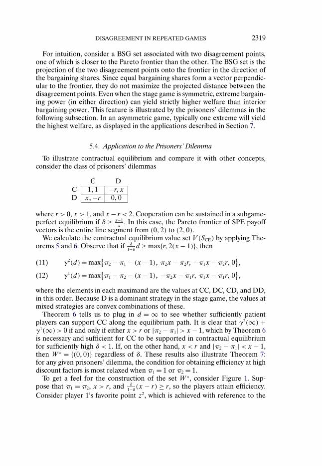
To get a feel for the construction of the set W ∗, consider Figure 1. Sup-pose that π1 = π2, x > r, and δ
1−δ(x − r) ≥ r, so the players attain efficiency.
Consider player 1’s favorite point z2, which is achieved with reference to the
2320 D. A. MILLER AND J. WATSON
FIGURE 1.—The prisoners’ dilemma with equal bargaining power. The parameters satisfyx > r and (π1�π2) = ( 1
2 �12 ). The endpoint z2 is attained by playing CC in the stage game and
using a transfer to split the surplus relative to the disagreement point w2. The disagreementpoint w2, in turn, is attained by playing DC in the stage game and continuing with promised util-ity v2 if no deviation occurs, but promised utility z2 if player 2 deviates. Minimizing z2
2 subjectto enforcing DC under disagreement and CC under agreement requires both v2
2 − z22 ≥ 1−δ
δr and
1 − z22 ≥ 1−δ
δ(x− 1).
disagreement point w2 that is furthest in the direction (π2�−π1) = ( 12 �− 1
2).In turn, w2 is the weighted average of u(DC) = (x�−r) and a point v2 ∈ W ∗.The former gets weight (1 − δ) and represents the payoff in the current pe-riod, whereas the latter has weight δ and gives the continuation payoff fromthe next period. Player 1 prefers that v2 be “pushed” down and to the right.However, v2 cannot equal z2 because there must be room to punish player 2 ifhe were to deviate from DC. If player 2 deviates, the continuation value z2 isselected; otherwise, the continuation value is v2. To discourage player 2’s devi-ation from DC, it must be that v2
2 −z22 ≥ 1−δ
δr. To support efficiency, it must also
be that 1−z22 ≥ 1−δ
δ(x−1) to discourage deviations from CC. The construction
is pictured in Figure 1.The contractual equilibrium set is intuitively satisfying in two key ways. First,
as Figure 1 demonstrates, contractual equilibrium yields a strict subset of the
DISAGREEMENT IN REPEATED GAMES 2321
Pareto frontier when CC is sustained along the equilibrium path.12 It can beshown that both endpoints of this subset shift toward higher payoffs for playeri when πi increases, so (conditional on sustaining CC on the equilibrium path)each player’s share of the available welfare is increasing (in a set-orderedsense) in his bargaining power. Second, contractual equilibrium has the ap-pealing property that equilibrium welfare decreases (weakly) as r increases,because higher r makes it more difficult to support play of DC or CD underdisagreement.
These properties contrast with the equilibria selected by renegotiation-proofness theories. Goldlücke and Kranz (2013; henceforth GK) showed thatif renegotiation is applied only before the transfer phase, then “strong optimal-ity” (Levin (2003)), “strong perfection” (Rubinstein (1980)), and “strong rene-gotiation proofness” (Farrell and Maskin (1989)) all select the entire Paretofrontier of SPE payoffs. For a discount factor of at least x−1
x, this is the line
segment between (0�2) and (2�0). Contractual equilibrium is more restrictive.For instance, in the case of π1 = π2 = 1/2, if x < r, then contractual equilib-rium selects only the value (0�0), regardless of the discount factor. If x ≥ r,then the lowest discount factor that supports CC in a contractual equilibriumis max{ r
x� 2x−2
3x−r−2 }, which strictly exceeds x−1x
, and in this case, contractual equi-librium selects a strict subset of the SPE Pareto frontier.13
Although none of the renegotiation refinements that GK studied allows fordisagreement, in terms of their equilibrium construction, one can construe arefusal to make a specified transfer as a disagreement. To illustrate, consider aGK equilibrium that sustains CC along the equilibrium path. If player 1 refusesto make a transfer, he is first punished with DD in the subsequent action phaseand then is required to make a transfer that yields him a zero payoff in thecontinuation. Since CC is still played in all future periods, the continuationpayoff vector under disagreement is (1 − δ)(0�2). If the players were able tobargain, their surplus in average terms would be δ2 > 0, and yet player 1 wouldcapture none of it—as if he had no bargaining power. That is, reconciling thisequilibrium with any notion of bargaining would require that all the bargainingpower be endogenously reallocated to whichever player is not being punished.Section 8.1 further discusses history-dependent bargaining power.
To illustrate how bargaining power influences the contractual equilibriumset, consider the prisoners’ dilemma when one player has all the bargaining
12Since w−ii ≥ 0 is required by individual rationality, πi > 0 implies z−i
i > 0.13Another approach in the renegotiation-proofness literature allows Pareto-dominated pun-
ishments as long as the players recognize that such punishments are needed to support high pay-offs at subsequent histories. For instance, the “consistent bargaining” theory of Abreu, Pearce,and Stacchetti (1993), which applies only to symmetric games, selects the best symmetric equi-librium from among those that maximize the minimum payoff any player earns at any history.Applying this notion prior to the transfer phase and, without loss of generality, employing sta-tionary “simple strategies” as defined by GK, yields a straightforward conclusion: the value set ofthe optimal consistent bargaining equilibrium converges to {(1�1)} as δ→ 1.
2322 D. A. MILLER AND J. WATSON
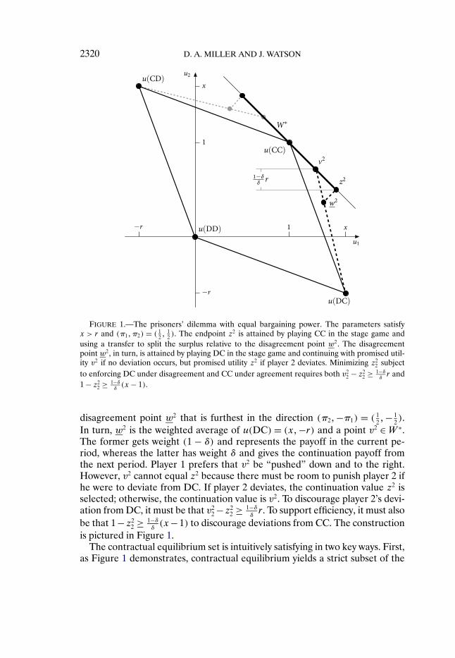
FIGURE 2.—The prisoners’ dilemma with unequal bargaining power. The parameters satisfyx < r, x < 2, and (π1�π2) = (1�0). Each endpoint zi is attained by playing CC in the stage gameand using a transfer to give player 1 all the surplus relative to the disagreement point wi . Thedisagreement point w2 is attained by playing DD in the stage game and continuing with promisedutility z2 regardless of whether a deviation occurs. The disagreement point w1 is attained byplaying CC in the stage game and continuing with promised utility v1 if no deviation occurs, butpromised utility zi if player i deviates unilaterally.
power, as illustrated in Figure 2. Suppose that x − r < 0 and x < 2; underthese conditions, if both players had equal bargaining power, then in con-tractual equilibrium they could attain only (0�0). But suppose instead thatπ1 = 1 = 1−π2. Then Γ (d)= γ1(d)= 2−x whenever δ
1−δd ≥ 2(x−1), because
γ2(d)= 0 for all d ≥ 0. State 2—which punishes player 2—uses DD under dis-agreement.14 Since player 2 has no bargaining power, she receives a payoffof zero under both agreement and disagreement. State 1 uses CC under bothdisagreement and agreement. This dramatically different construction arisesbecause CC and DD are relatively cheap in terms of incentives (because x < r,
14Strictly speaking, there is an indeterminacy in state 2 behavior under disagreement—thearg max of γ2 includes both DC and DD when π2 = 0. However, only DD arises along any se-quence with π2 > 0 and π2 → 0.
DISAGREEMENT IN REPEATED GAMES 2323
CD and DC are very expensive), and their projections onto the Pareto frontierin the direction of the bargaining power are widely separated.
These results show that contractual equilibrium generates specific predic-tions for the prisoners’ dilemma, including predictions that distinguish it fromrenegotiation proofness.
6. GENERALIZATION
This section extends our analysis to a general model with more than twoplayers, imperfect public monitoring, and heterogeneous discount factors. Forsimplicity, we do not specify the bargaining process, but instead assume thatthere exist bargaining weights that summarize the relevant backward inductionsolution of the bargaining phase under the axioms. (It would be cumbersome,but straightforward, to construct such a bargaining process using a generalizedalternating-offer protocol.15) A simplified description of a game in this class isa tuple 〈n� A�Θ� f�u�δ�π〉, with the following components:
• A finite number of players n.• A stage game, featuring a set of action profiles A = A1 × · · · × An, a set
of public signals Θ, a signal distribution function f : A → �Θ, and payoff func-tions (ui : Ai ×Θ → R)ni=1.
• A vector of discount factors δ ∈ [0�1)n, where δi denotes player i’s dis-count factor.
• Bargaining weights π = (π1�π2� �πn), with π ≥ 0 and∑n
i=1 πi = 1.In the stage game, the players simultaneously select their actions, yielding ac-tion profile a ∈ A. Public signal θ ∈ Θ is then realized according to the proba-bility measure f (·|a). The players publicly observe θ, but they do not observeeach other’s actions. We write u(a�θ) ≡ (ui(ai� θ))
ni=1, and extend f and u to
the space of mixed actions. We examine a “perfect public” notion of contrac-tual equilibrium in which the disagreement point and all individual actions areconditioned on only the public history.
Since utility in average terms is no longer necessarily transferable, we ex-press continuation payoffs in total terms rather than average terms. To makethe difference clear in notation, values that were in average terms in previoussections but are now in total terms are shown with a tilde. The construction of acontinuation value w from the negotiation phase must now incorporate (i) con-tinuation values as a function of the public signal and (ii) the players’ possiblydifferent discount factors. For any two vectors x�x′ ∈ R
n, define the compo-nentwise multiplication operator ∗ as x ∗ x′ ≡ (x1x
′1�x2x
′2� � xnx
′n). We use
the standard notation x · x′ for the dot product of x and x′, and define 1 as
15Alternating-offer bargaining games with three or more players can have many equilibria. Themultiplicity can be resolved by selecting the unique Markov-perfect equilibrium in the isolatedbargaining game, which can be viewed as imposing NFD on each round of bargaining rather thanmerely after bargaining breaks down.
2324 D. A. MILLER AND J. WATSON
the n-dimensional vector of ones. Then an agreement continuation value w isconstructed as
w = m+∫θ∈Θ
(u(α�θ)+ δ ∗ g(θ)
)df(θ|α)�(13)
where m ∈ Rn0 ≡ {m′ ∈ R
n|∑n
i=1 m′i = 0} is the transfer, α ∈ �A is the mixed
action profile, g(θ) is the continuation value from the start of the next periodfollowing public signal θ, and f (θ|α) is the probability measure on Θ that arisesfrom α. Similarly, a disagreement value is given by
w =∫θ∈Θ
(u(α�θ)+ δ ∗ g(θ)
)df(θ|α)(14)
We say that g :Θ→ W enforces α if α is a Nash equilibrium of the game withaction-profile space A and payoffs given by
∫θ∈Θ(u(a�θ) + δ ∗ g(θ))df (θ|a).
Operators D, C, and B are revised as
D(W ) ≡ {w ∈ R
n∣∣(15)
∃ g :Θ→ W and α ∈ �As.t. g enforces α and Eq. (14) holds
}�
C(W )≡ {w ∈ R
n∣∣(16)
∃m ∈ R20 and w′ ∈ D(W )
s.t. w =m+ w′ and w ∈D(W )}�
where D is defined as before, and
B(W � W )≡{w +π
(maxw′∈W
1 · w′ − 1 · w) ∣∣∣ w ∈ W
}(17)
As before, W is a BSG set if W = coB(C(W )�D(W )); the definition of fullPareto dominance carries over unchanged as well.
With A and Θ finite, we can guarantee existence.
THEOREM 8: Consider any n-player game in the simplified form 〈n� A�Θ� f�u�δ�π〉. If A and Θ are finite and δi ∈ [0�1) for all i, then the game has a uniquedominant BSG set W ∗. Moreover, W ∗ is a compact hyperpolygon contained in ahyperplane normal to the vector 1.
The proof, given in Appendix B.2 in the Supplemental Material, examinesa fixed-point problem for a transformation of the self-generation operatorcoB(C(·)�D(·)). The transformation normalizes the set of continuation values
DISAGREEMENT IN REPEATED GAMES 2325
by subtracting the welfare level in a direction that accounts for the heteroge-neous discount factors and bargaining shares. Since the normalized bargain-ing operator preserves compactness, and is bounded, monotone, and continu-ous on decreasing sets, Tarski’s fixed-point theorem guarantees a largest fixedpoint—which is a hyperpolygon in R
n.For the special case of two players, V (SCE) can be explicitly characterized
even allowing for imperfect public monitoring and asymmetric discount factorsδ = (δ1� δ2). As in Section 5.1, the contractual equilibrium set is a compact linesegment of slope −1, where each endpoint is an agreement value formed withreference to an appropriately chosen disagreement point. Since the heteroge-neous discount factors impose significant extra notation, we reserve the gorydetails for Appendix B.2.
For symmetric games, a small disparity in discount factors has a similar ef-fect to a small disparity in bargaining power: as the following corollary shows,the more patient player gains and the less patient player loses, but in averageterms, the gains outweigh the losses. Let zi ≡ 1
2(1−δi)(z1
i + z2i ), that is, player i’s
average payoff across the two states, in average terms. Let z = 12(z1 + z2), that
is, the average welfare across the two states, in average terms.
COROLLARY 2: If the stage game is symmetric and π = ( 12 �
12), then, fixing the
average discount factor, z strictly increases in any sufficiently small disparity be-tween the discount factors, while the less patient player’s average payoff across thetwo states strictly decreases.
7. APPLICATION TO RELATIONAL CONTRACTING
In this section, we use contractual equilibrium to examine the role of bar-gaining power in a principal-agent relationship and to explore the impact of ex-ternal enforcement. We then comment on possible connections with the macrolabor literature.
7.1. A Principal-Agent Problem
We first investigate the role of bargaining power in the context of a principal-agent model with moral hazard, based on Levin (2003). We find that the agent’seffort is increasing in his bargaining power and that the principal prefers anintermediate level of bargaining power.
In each stage game, the agent chooses effort e ∈ [0� e], incurring a cost c(e),and then the principal makes a voluntary payment to the agent. The principal’srevenue is a random variable θ, with probability density f (·|e) and full sup-port on a compact interval. The expected payoff vector in the stage game (i.e.,excluding transfers) is u(e) = (−c(e)�
∫θdf (θ|e)). The principal does not ob-
serve e, but θ is public, so the principal’s voluntary payment can be conditioned
2326 D. A. MILLER AND J. WATSON
on θ. We assume that c is strictly increasing and strictly convex, c(0)= 0, f hasthe monotone likelihood property,
∫θdf (θ|0) = 0, and f (θ|e = c−1(·)) is con-
vex. The players engage in bargaining and can make voluntary transfers beforethe stage game in each period, and they share a common discount factor δ < 1.We normalize payoffs by (1 − δ) to put them in average terms.
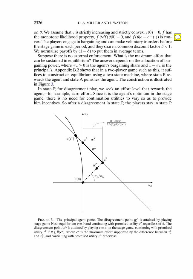
Suppose there is no external enforcement. What is the maximum effort thatcan be sustained in equilibrium? The answer depends on the allocation of bar-gaining power, where πA ≥ 0 is the agent’s bargaining share and 1 − πA is theprincipal’s. Appendix B.2 shows that in a two-player game such as this, it suf-fices to construct an equilibrium using a two-state machine, where state P re-wards the agent and state A punishes the agent. The construction is illustratedin Figure 3.
In state P, for disagreement play, we seek an effort level that rewards theagent—for example, zero effort. Since it is the agent’s optimum in the stagegame, there is no need for continuation utilities to vary so as to providehim incentives. So after a disagreement in state P, the players stay in state P
FIGURE 3.—The principal-agent game. The disagreement point wP is attained by playingstage-game Nash equilibrium e = 0 and continuing with promised utility zP regardless of θ. Thedisagreement point wA is attained by playing e = e∗ in the stage game, continuing with promisedutility zP if θ ≥ θ(e∗), where e∗ is the maximum effort supported by the difference between zP
Aand zA
A, and continuing with promised utility zA otherwise.
DISAGREEMENT IN REPEATED GAMES 2327
the following period regardless of the realized output. Under agreement instate P, the players recognize that their “outside option” is to disagree, im-plement zero effort, and then return to state P next period. Therefore, theirutility (specifically, their vector of average discounted utilities) under disagree-ment is a convex combination of (0�0) and their agreement utility in state P.Since the agent obtains a πA fraction of the surplus, their agreement utilityis (πA�1 − πA) · (E(θ|e∗) − c(e∗)), where e∗ is the equilibrium path effort. Toattain this utility, the principal makes a payment to the agent as part of theiragreement. The principal is willing to pay because doing so gives her strictlyhigher utility than does the disagreement that would arise should she fail topay.
In state A, we seek an effort level under disagreement that punishes theagent. The best candidate is the equilibrium path effort e∗, which is the highesteffort that can be enforced using equilibrium continuation utilities. This effortlevel is enforced by staying in state A for low realizations of θ and transitingto state P for high realizations of θ.16 As Levin showed, the optimal cutofffor enforcing effort level e∗ is the output level θ(e∗) at which ∂
∂ef (θ|e)|e=e∗ ,
as a function of θ, switches from negative to positive (by the monotone likeli-hood property, this identifies a unique output level). In fact, this same incentivescheme must be used whenever the agent is to exert effort e∗, that is, in state Punder agreement as well as in state A under both agreement and disagreement.
Since optimal effort is played under disagreement in state A, disagreement isalready on the Pareto frontier of what is attainable in equilibrium. Hence thereis no surplus to share, so play is the same under agreement and disagreement.Because the agent can always deviate to zero effort in every period, his utilityin state A must be at least zero. To provide the maximal incentives, in fact hisutility in state A should be exactly zero.
Equilibrium path effort e∗ is thus a fixed point of the agent’s optimizationproblem:17
e∗ ∈ arg maxe∈[0�e]
(−(1 − δ)c(e)(18)
+ δPr(θ ≥ θ
(e∗)∣∣e)πA
(E(θ|e∗) − c
(e∗)))
Because the principal and the agent negotiate over how to play, they will jointlyselect the highest fixed point. Since incentives are stronger the more weightthe agent places on the second term in his objective function, we see that e∗
increases in δ and πA, and converges to efficient effort as δ→ 1 and πA → 1.
16If the principal could promise a voluntary payment for high realizations of θ in the actionphase, it would have the same effect as transitioning to state P.
17We assume for convenience that e ∈ arg maxe∈[0�e][E(θ|e)− c(e)], so inefficiently high effortis infeasible.
2328 D. A. MILLER AND J. WATSON
Observe that only zero effort is supported if the principal has all the bar-gaining power (πA = 0). Suppose that the agent exerts zero effort if the playershave never agreed; then their agreement in the first period selects zP as theirinitial payoffs. In that case, the principal also receives zero utility if she hasno bargaining power (πA = 1), so her utility is nonmonotone in πA. An insti-tution that selects a Pareto-optimal bargaining protocol will always endow theagent with some bargaining power, leading the agent to earn payoffs strictlyhigher than zero, that is, an internal efficiency wage. In particular, the princi-pal will prefer to have more bargaining power for herself when it is easier tomotivate the agent—such as when the discount factor is higher, when outputis less noisy (holding the expected returns to effort fixed), or when there is anadditional signal that is informative about the agent’s effort.
Levin’s “strongly optimal” equilibrium relies on continuation play that, fol-lowing an out-of-equilibrium offer by the principal, punishes the principal ifthe agent rejected but punishes the agent if the agent accepted. Since the dis-agreement outcome is sensitive to the manner of disagreement, there is littlerole for the exercise of bargaining power. In contractual equilibrium, in con-trast, NFD ensures a well-defined default point for bargaining each period,while internal and Pareto external agreement consistency allow the agents toendogenously select a division of the surplus that accords with their bargainingpower.
7.2. External Enforcement and Self-Enforcement
To further illustrate the usefulness of contractual equilibrium, this sectionconsiders the question posed by Baker, Gibbons, and Murphy (1994; hence-forth BGM): Does external enforcement help or harm self-enforcement?BGM focused on “trigger punishments” in which the agent punishes the prin-cipal for reneging on a voluntary payment by refusing to accept “implicit”(self-enforced) contracts offered in the future. When “explicit” (externallyenforced) contracts are available, BGM assumed that even in a trigger pun-ishment, the agent would accept an externally enforced contract and, there-fore, the principal offers the externally enforced contract that maximizes herprofit.18 BGM’s key insight is that the threat of terminating the relationshipis a more severe punishment than reverting to profit-maximizing externallyenforced contracts and can, therefore, support higher payoffs in equilibrium.Thus, BGM found that externally enforced and self-enforced contracts can besubstitutes.
18BGM adopted this assumption “because the purely game-theoretic analyses of renegotiationabstract from institutions that would influence renegotiation in the labor market we consider.”By explicitly modeling the bargaining process, our framework provides tools that answer thischallenge.
DISAGREEMENT IN REPEATED GAMES 2329
In contrast, recent empirical studies find complementarity between exter-nally enforced and self-enforced contracts: better external enforcement im-proves the ability of partners to self-enforce their agreements (Beuve andSaussier (2012), Lazzarini, Miller, and Zenger (2004), Ryall and Sampson(2009)). We show here that complementarity follows generally from the analy-sis of contractual equilibrium.
A trigger punishment (either termination or reversion to only explicit con-tracts) is generally not viable under agreement in contractual equilibrium, be-cause the principal and the agent can bargain their way out of it. Likewise, anexplicit “spot market” contract of the sort considered by BGM would not ariseunder disagreement in contractual equilibrium, because it requires the agree-ment of both parties. That is, an externally enforced contract cannot serve asthe players’ “fallback position” unless it is already in place prior to bargaining.Thus, the fallback position is continued interaction under the parties’ initiallong-term contract (the employment contract).
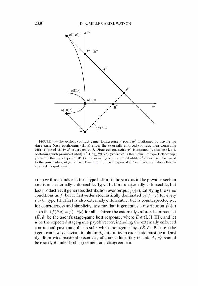
To broaden our results, we generalize the model from Section 7.1 to allowfor external enforcement of some less productive form of effort. At first, wetake the externally enforced contract to be given exogenously; we discuss laterhow it might be chosen endogenously. We find that when the agent has somebargaining power, the availability of external enforcement always improves theprospects for self-enforcement. In particular, an optimal long-term externallyenforced contract induces the agent to exert counterproductive effort by com-pensating him for his verifiable effort costs. This externally enforced contract isalways undone by self-enforced incentives under agreement; it directly drivesonly behavior under disagreement. A surplus-destroying externally enforcedcontract raises the stakes of bargaining when the agent is rewarded, enablingthe agent to capture more of the surplus. When the agent is being punished, thesame behavior is implemented under disagreement and agreement, so there isno surplus to bargain over. Compared to the case without external enforce-ment, the difference in the agent’s payoff under agreement in the two states isgreater, supporting higher effort on the equilibrium path.19
The contractual equilibrium we describe is similar to that outlined in Sec-tion 7.1 and is illustrated in Figure 4. In state P under disagreement, the prin-cipal pays only to the letter of the externally enforced contract and the agentplays his stage-game best response. In state A under disagreement and in bothstates under agreement, the agent plays his equilibrium-path effort, and is op-timally rewarded by transiting to state P for good outcomes and is punished bytransiting to state A for bad outcomes.
Suppose that the agent chooses both the kind and the level of his effort. Asbefore, his effort level is e ∈ [0� e] and his effort cost is c(e). However, there
19Kvaløy and Olsen (2009) found that relational contracting is strengthened when parties agreeon a breach remedy that minimizes surplus. In their model, breach is triggered by a deviation inthe action phase and leads to a trigger punishment in which bargaining is disallowed.
2330 D. A. MILLER AND J. WATSON
FIGURE 4.—The explicit contract game. Disagreement point wP is attained by playing thestage-game Nash equilibrium (III� e) under the externally enforced contract, then continuingwith promised utility zP regardless of θ. Disagreement point wA is attained by playing (I� e∗),continuing with promised utility zP if θ ≥ θ(I� e∗) (where e∗ is the maximum type I effort sup-ported by the payoff span of W ∗) and continuing with promised utility zA otherwise. Comparedto the principal-agent game (see Figure 3), the payoff span of W ∗ is larger, so higher effort isattained in equilibrium.
are now three kinds of effort. Type I effort is the same as in the previous sectionand is not externally enforceable. Type II effort is externally enforceable, butless productive: it generates distribution over output f (·|e), satisfying the sameconditions as f , but is first-order stochastically dominated by f (·|e) for everye > 0. Type III effort is also externally enforceable, but is counterproductive:for concreteness and simplicity, assume that it generates a distribution f (·|e)such that f (θ|e) = f (−θ|e) for all e. Given the externally enforced contract, let(E� e) be the agent’s stage-game best response, where E ∈ {I� II� III}, and letu be the expected stage-game payoff vector, including the externally enforcedcontractual payments, that results when the agent plays (E� e). Because theagent can always deviate to obtain uA, his utility in each state must be at leastuA. To provide maximal incentives, of course, his utility in state A, zA
A, shouldbe exactly u under both agreement and disagreement.
DISAGREEMENT IN REPEATED GAMES 2331
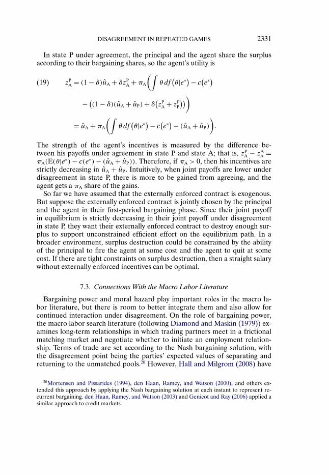
In state P under agreement, the principal and the agent share the surplusaccording to their bargaining shares, so the agent’s utility is
zPA = (1 − δ)uA + δzP
A +πA
(∫θdf
(θ|e∗) − c
(e∗)(19)
− ((1 − δ)(uA + uP)+ δ
(zP
A + zPP
)))
= uA +πA
(∫θdf
(θ|e∗) − c
(e∗) − (uA + uP)
)
The strength of the agent’s incentives is measured by the difference be-tween his payoffs under agreement in state P and state A; that is, zP
A − zAA =
πA(E(θ|e∗)− c(e∗)− (uA + uP)). Therefore, if πA > 0, then his incentives arestrictly decreasing in uA + uP. Intuitively, when joint payoffs are lower underdisagreement in state P, there is more to be gained from agreeing, and theagent gets a πA share of the gains.
So far we have assumed that the externally enforced contract is exogenous.But suppose the externally enforced contract is jointly chosen by the principaland the agent in their first-period bargaining phase. Since their joint payoffin equilibrium is strictly decreasing in their joint payoff under disagreementin state P, they want their externally enforced contract to destroy enough sur-plus to support unconstrained efficient effort on the equilibrium path. In abroader environment, surplus destruction could be constrained by the abilityof the principal to fire the agent at some cost and the agent to quit at somecost. If there are tight constraints on surplus destruction, then a straight salarywithout externally enforced incentives can be optimal.
7.3. Connections With the Macro Labor Literature
Bargaining power and moral hazard play important roles in the macro la-bor literature, but there is room to better integrate them and also allow forcontinued interaction under disagreement. On the role of bargaining power,the macro labor search literature (following Diamond and Maskin (1979)) ex-amines long-term relationships in which trading partners meet in a frictionalmatching market and negotiate whether to initiate an employment relation-ship. Terms of trade are set according to the Nash bargaining solution, withthe disagreement point being the parties’ expected values of separating andreturning to the unmatched pools.20 However, Hall and Milgrom (2008) have
20Mortensen and Pissarides (1994), den Haan, Ramey, and Watson (2000), and others ex-tended this approach by applying the Nash bargaining solution at each instant to represent re-current bargaining. den Haan, Ramey, and Watson (2003) and Genicot and Ray (2006) applied asimilar approach to credit markets.
2332 D. A. MILLER AND J. WATSON
criticized this assumption as unrealistic. Their point is that if separation is vol-untary, then the disagreement point should be defined not as the parties’ sep-aration values, but as their continuation values in their current relationship—including the possibility, but not the requirement, of separation.
On moral hazard, workers can be motivated by “efficiency wages” that theywould lose if fired from their jobs. Following Shapiro and Stiglitz (1984), tra-ditional efficiency wage models assume that firms commit to a constant wage,so there is no ongoing bargaining between firms and workers. More recently,the relational contracts literature has started to address the question of howfirms can commit endogenously to wage schedules that may vary with outputor other monitoring signals. However, in these models, bargaining power ei-ther does not play a role (e.g., MacLeod and Malcomson (1989, 1998), Levin(2003)) or is applied only at the beginning of the relationship (e.g., Ramey andWatson (1997, 2001), Moen and Rosén (2011)).
Our analysis indicates that the institutional setting that underlies bargainingpower may influence the returns to the employment relationship, because theworker’s payoffs both on the equilibrium path and after a deviation (the differ-ence between which constitutes the effective efficiency wage) are endogenouslyselected through the bargaining process. This is important not only when themoral hazard problem concerns the worker’s efforts, but also where it concernshis investments, such as in human capital.21 It may be useful to empiricallyevaluate aspects of productive relationships that are influenced by bargainingpower, and also find ways to measure bargaining power directly. Regarding thelatter, at the industry or firm level, one might associate bargaining power withthe level of unionization. For instance, Dobbelaere (2004) found that the to-tal surplus divided between the firm and workers is positively correlated withunionization, which is consistent with our principal-agent example. In a relatedcase study, Guy (2003) suggested that initiation of a customer service programincreased the workers’ bargaining power, resulting in better effort incentives,but also greater rents for the workers. Though these results may be suggestive,further research is needed to help understand the relationship between collec-tive bargaining power at the union level and the moral hazard problems thatplay out primarily at the level of an individual worker.
8. CONCEPTUAL DISCUSSION
This section discusses links between our approach and the prior literatureson preplay communication and renegotiation proofness. We comment on theimplications of varying the axioms and the structure of the model, and discussconnections with experimental work.
21In principle, these interrelationships could affect the propagation of shocks in macro labormodels; see den Haan, Ramey, and Watson (2000) as well as Rogerson, Shimer, and Wright(2005) and Ramey (2011) for surveys of the literature.
DISAGREEMENT IN REPEATED GAMES 2333
8.1. Positive Foundations for Bargaining
Our axioms have antecedents in the literature on preplay communication.Farrell (1987, 1988) allowed players to make cheap-talk announcements beforechoosing their payoff-relevant actions. Farrell looked at symmetric equilibriawith the properties that (i) if the announced actions constitute an equilibriumin the second-stage subgame, then the players will select this action profile inthe second stage; (ii) otherwise, the players will select an arbitrary equilibriumof the subgame. If one construes Farrell’s condition (i) as “agreement” andcondition (ii) as “disagreement,” then our IAC and PEAC axioms relate toFarrell’s first assumption, and our NFD axiom relates to his second assump-tion. Santos (2000) built on Farrell’s approach by structuring the cheap-talkphase as a bargaining process and showed that inefficient Nash equilibria canarise if players condition their play in the subgame on the way in which dis-agreement occurs—a theme continued with our Theorem 1. But only efficientNash equilibria arise if the players do not condition on the history of messagesin disagreement (a precursor of NFD).22
As in the preplay communication literature, the positive justification for ouraxioms is to allow the players to meaningfully discuss how to play. An axiomaticapproach is necessary, because, as in any cheap-talk model, “babbling” is al-ways a possibility; that is, the players could simply ignore all communicationand bargaining would be meaningless. Accordingly, our axioms on the mean-ing of agreement—IAC and PEAC—imply that players mean what they saywhen they propose and accept certain kinds of offers.
IAC and PEAC are weaker than renegotiation-proofness axioms in that theymerely make these continuation equilibria available for the players to dis-cuss, rather than require the players to accept them. Holding aside this differ-ence, however, IAC and PEAC have direct counterparts in the renegotiation-proofness literature. Specifically, IAC makes available for discussion any con-tinuation play that is decomposable on the set of payoffs available at other his-tories in the same equilibrium, as contemplated by Ray’s (1994) notion of “in-ternal renegotiation proofness.” It also relates closely to the “internal consis-tency” notion of Bernheim and Ray (1989) and the “weak renegotiation proof-ness” notion of Farrell and Maskin (1989).23 Similarly, PEAC makes available
22Watson (1991), Rabin (1994), and Arvan, Cabral, and Santos (1999) also built on Farrell’smodel. Watson (2006) provided a general treatment that embeds bargaining in finite-horizongames.
23Pearce (1987) critiqued these notions as follows: If the players find themselves in a punish-ment that is Pareto dominated by play at some other history, but the payoffs obtained at that otherhistory are supported by the threat of a punishment similar to the one they currently face, thenthe idea that they could renegotiate to that other history is a contradiction. Internal consistencyand related notions resolve the contradiction by invalidating the equilibrium, but Pearce (and,subsequently, Asheim (1991), Abreu, Pearce, and Stacchetti (1993), and Bergin and MacLeod(1993)) resolved the contradiction by invalidating the proposal. We do not mean to take a strong
2334 D. A. MILLER AND J. WATSON
for discussion continuation play available in “better” equilibria, where oneequilibrium is “better” than another if the value set of the first fully Paretodominates the value set of the second. Since such equilibria are not vulnera-ble to Pareto-improving deviations back to the current equilibrium, PEAC’sclosest counterpart in the renegotiation-proofness literature is the “stationaryPareto perfection” notion of Asheim (1991).
A theory of disagreement is necessary because IAC and PEAC alone have nobite—it does not matter how players interpret agreements if there is no notionof how they should interpret disagreement. Our theory of disagreement, em-bodied in the NFD axiom, endows the bargaining phase with a well-defineddisagreement point, which in turn allows the players’ behavior to be inter-preted in the context of the canonical alternating-offer bargaining paradigm.This paradigm is positively appealing because its backward induction solutionis sensitive to both bargaining power (derived from the bargaining protocol)and the disagreement outcome. The backward induction solution also has nor-mative foundations in static settings, since it is equivalent to the weighted Nash(1950) bargaining solution.
Still, it is not obvious that NFD is positively appealing in repeated settings:Would the other players not bear a grudge against, and single out for pun-ishment, a player who deviates by offering to take a larger share for himself?We are sympathetic toward this critique. But the critique alone does not iden-tify what the equilibrium offer should be in the first place. In fact, the cri-tique leaves open the possibility that even a deviant offer that strictly Paretodominates the equilibrium offer could engender a grudge and thereby be dis-couraged. A more finely tuned “theory of grudges” would indicate what kindsof deviant offers should engender grudges when bargaining breaks down. De-pending on the details, such a theory might generate testable predictions thatcould distinguish it from NFD.
Our theory of disagreement could be modified to accommodate a limitednotion of grudges without affecting our results. What is important about NFDis that no offer on the Pareto frontier of either V (s) or V (SCE) should engen-der a grudge if it also Pareto dominates the disagreement point. If the bar-gaining phase outcome is to be summarized using the Nash bargaining solu-tion, a responder considering such an offer must evaluate it with respect tothe same disagreement point that would obtain if he rejected the equilibriumoffer. Other offers can engender grudges without disrupting the equilibriumbargaining outcome.
Other notions of disagreement are also potentially fruitful. The renego-tiation-proofness literature, although it does not address the possibility of dis-
philosophical stand on this question. Indeed, imposing merely NFD and a variant of PEAC, with-out IAC, would yield a coherent theory of equilibrium selection, but one that is beyond the scopeof this paper.
DISAGREEMENT IN REPEATED GAMES 2335
agreement,24 could be interpreted as imposing the theory that play under dis-agreement is identical to that under agreement. An alternative way to reconcilerenegotiation proofness with our framework is to impose NFD and one or bothconsistency axioms, but allow the players’ relative bargaining power to dependon the history. Allowing the bargaining weights to vary in arbitrary ways wouldenable the players to reach agreement on any point on the Pareto frontier ofC(W ) as long as it Pareto dominated the disagreement point. For instance, theresults of Levin (2003, discussed in Section 7.1) could be reconciled with ouraxioms if the agent got to make the take-it-or-leave-it offer in his reward state,but the principal got to make the offer in the agent’s punishment state. How-ever, it is our view that bargaining power should be derived from primitives ofthe model rather than treated as an aspect of equilibrium selection.
For symmetric games, Abreu, Pearce, and Stacchetti (1993) proposed a no-tion of “consistent bargaining equilibrium” that maximizes the minimum con-tinuation payoff that any player can receive after any history, rather than im-posing internal consistency. The bargaining process that generates their theorycan be loosely conceptualized as follows. Each player has veto power over con-tinuation play; if player i exercises his veto, then they revert to a symmetricequilibrium of his choice, but starting from whichever history yields player i’sworst continuation payoff in that equilibrium. This notion violates NFD, sincecontinuation play following a veto depends on who exercised the veto.25 Abreu,Pearce, and Stacchetti interpreted veto power as a kind of equal bargainingpower. They cautioned, however, that their notion should not be viewed as a“definitive solution,” and challenged the literature to generate an “authorita-tive bargaining theory for the division of surplus in repeated games.” Contrac-tual equilibrium is our answer to this challenge.
8.2. The Timing of Transfers and Bargaining
In our modeling approach, the players bargain and then make voluntarytransfers at the beginning of each period, and, by the NFD axiom, coordinateto make no transfers under disagreement. One way to interpret these assump-tions is that, in reality, the monetary transfer marks the successful resolution ofbargaining: If the agreement involves an immediate transfer—one player writ-ing a check payable to the other—then it is the signature on the check, ratherthan the verbal “yes,” that signifies the successful resolution of bargaining. Fail-
24One exception is Blume (1994), who allowed the players to agree to a plan that involvesPareto-dominated continuation values in the future. Blume’s approach gives the players surplusto bargain over, but does not model bargaining power or investigate its implications. In principle,Blume’s formal structure leaves open the possibility of modeling bargaining power by imposingaxioms on the bargaining operator he defined.
25It is unclear how to resolve coordination problems that would arise when either multipleplayers wish to veto or each player would prefer that other players exercise their vetoes.
2336 D. A. MILLER AND J. WATSON
ing to write the check implies disagreement. In this sense, the bargaining phaseencompasses the transfer choices.26
Still, it could be interesting to consider variations on the timing of trans-fers and bargaining within a period. In the renegotiation-proofness literature,Baliga and Evans (2000) studied transfers that occur simultaneously with ac-tions, while GK and Fong and Surti (2009) studied transfers that occur in aseparate phase. In the context of contractual equilibrium, consider what couldhappen after a player reneges on an agreed-upon transfer. If there is no bar-gaining between the transfer and action phases, the players’ continuation valuemay be any point in D(W ), the set of payoffs attainable from the action phase.In contrast, if there is an additional bargaining phase before the action phase,then the players should agree to continuation play on the Pareto frontier ofD(W ). Depending on the stage game and the discount factor, this additionalconstraint may or may not restrict the set of attainable payoffs, as shown byGK.
Finally, what if there were no transfer phase between the bargaining and ac-tion phases, for example, if all transfers occurred simultaneously with actions?Contractual equilibrium would still constitute a coherent theory of equilib-rium selection, but one would have to specify whether disagreement impliesany restriction on how players coordinate their play in the action phase (suchas no transfers). Without such a restriction, the C and D operators would beidentical, so given any contractual equilibrium, one could always modify playunder disagreement to be identical to play under agreement. There wouldbe no surplus to bargain over, so bargaining power would play no role. Theimplications of contractual equilibrium would be similar to those of “consis-tent” equilibrium (Bernheim and Ray (1989)). In our model, surplus arisesfrom the fact that the Pareto frontier is higher under agreement than underdisagreement. For the study of relational contracts, we argue that transfersand productive actions are most appropriately modeled in separate phases,and that forcing them to occur simultaneously constitutes a knife-edge specialcase.
8.3. Experimental Connections
The experimental setting presents a good opportunity to develop intuitionand test the predictions of contractual equilibrium against other theories. Weare not aware of experiments on recurrent bargaining in infinitely repeatedgames. However, some experimental work on preplay communication and co-ordination relates to key elements of our theory.
Experiments on preplay communication suggest that players use messagesto coordinate their behavior, and that the protocol by which they communi-
26Checks require a minimal degree of external enforcement. Our approach readily generalizesto settings in which other types of contractual clauses may also be externally enforceable.

DISAGREEMENT IN REPEATED GAMES 2337
cate imparts a measure of bargaining power. For example, Cooper, DeJong,Forsythe, and Ross (1989, 1992) compared games with one-way and two-waycommunication. With one-way communication, the sender typically announceshis preferred equilibrium of the underlying game and the players typically playthis equilibrium. With simultaneous two-way communication, outcomes aremore symmetric, but the players often fail to coordinate. Allowing multiplerounds of simultaneous messages reduces the incidence of coordination fail-ure.27
Cooper and Kühn (2013) provided provocative evidence on communication,coordination, and renegotiation in games. Cooper and Kühn conducted two-period experiments and studied the effect of allowing or disallowing commu-nication between periods. Cooperation in the first period is more frequentwhen a player has threatened to use second-period play to punish a cheater(by coordinating on a Pareto-dominated equilibrium), suggesting that playersuse preplay communication to coordinate. Moreover, when players can com-municate between periods, they often renegotiate away from punishments toselect a Pareto-dominant equilibrium in the second period, as would be pre-dicted by both our theory and renegotiation proofness. Nonetheless, cooper-ation in the first period is even higher with between-period communication.Players take the opportunity between periods to admonish one another (some-times aggressively) for cheating in the first period. Cooper and Kühn inter-preted these admonishments as nonpecuniary punishments that may be lesscostly to the admonisher than punishing via actions in the second-period stagegame.
Clear distinctions between contractual equilibrium and renegotiation proof-ness do not arise in the results of Cooper and Kühn, because their experimentaldesign does not allow for monetary transfers, variations in relative bargainingpower, or variations in stage-game payoffs.28 However, we can suggest a re-lated experiment to test the distinct predictions of contractual equilibrium. Wepropose an experiment with the following features: (i) the players can makevoluntary transfers between the two periods; (ii) the second-period coordina-tion game has a Pareto-dominant Nash equilibrium, but also has asymmetricPareto-dominated equilibria; (iii) communication between periods follows aspecific bargaining protocol.29 Varying the equilibrium payoffs of the coordi-nation game would produce different disagreement values and surpluses. By
27See Crawford (1998) for a description of this and other cheap-talk experiments.28Sloof and Sonnemans (2011) studied the Schmidt and Schnitzer model with communica-
tion and transfers. However, the experimental design focuses on technology choice rather thanbargaining, and so does not separate the Schmidt and Schnitzer model from standard subgame-perfection analysis.
29Players might engage in less verbal admonishment when they have access to monetary trans-fers as an even cheaper punishment instrument, in addition to multiple equilibria to use as dis-agreement points.
2338 D. A. MILLER AND J. WATSON
varying the bargaining protocol, one could look at different degrees of rela-tive bargaining power. Contractual equilibrium predicts that these variationsshould matter for supporting cooperation in the first period. It may also beuseful to have noisy play in the first period, so that it is not known whetherdeviations from an agreement were intentional.
9. CONCLUSION
This paper introduces contractual equilibrium, a new approach to equilib-rium selection in repeated games that is based on communication with endoge-nous meaning. Contractual equilibrium allows disagreement play and bargain-ing power to arise endogenously, in a way consistent with a well-defined ex-tensive form. Contractual equilibrium exists, yields a unique welfare level, istractable in applications, and extends easily to games with imperfect monitor-ing and heterogeneous discount factors.
The underlying principles of contractual equilibrium are not restricted to re-peated games with transfers. In dynamic games, where a payoff-relevant statecan vary over time and shift endogenously in response to players’ actions, thesame notions of agreement and disagreement apply. Endogenous disagree-ment can be particularly powerful in a dynamic setting, since the actions takenunder disagreement can change the set of feasible continuation values.30 Fi-nally, it would be interesting to consider how disagreement play might dependon which coalitions manage to cohere when the grand coalition fails to agree.We view all of these extensions as promising areas for further research.
Since the noncooperative solution of the generalized alternating-offer bar-gaining game under our axioms is expressed in terms of bargaining power, ityields the same outcome as the generalized Nash bargaining solution. Hencethe same conclusions would arise from a hybrid model in which the noncoop-erative bargaining and transfer phases are replaced with a cooperative Nashbargaining phase.31
30The legal environment—the set of enforceable contracts and the enforcement technology—can introduce dynamics if long-term contracts are enforceable. Then the players’ signatures onthe contract, though they have no effect on the feasibility of the equilibrium path since the con-tract can always be renegotiated, can leverage the threat of enforcement to change the feasibleset of continuation values after future disagreements.
31There is a tradition of incorporating cooperative bargaining into otherwise noncooperativegames to model bargaining power. One example is the macroeconomic literature on labor marketsearch frictions, as discussed in Section 7.3. Another is the holdup theory of the firm originatedby Grossman and Hart (1986) and Hart and Moore (1990). Schmidt and Schnitzer (1995) andRamey and Watson (2002) employed a hybrid approach to relational contracts. Harrington (1989)and Brandenburger and Stuart (2007) examined the actions that take place leading up to anagreement, where the agreement yields a contract that terminates the game.
DISAGREEMENT IN REPEATED GAMES 2339
APPENDIX A: PROOFS
A.1. No-Bite Theorems
We expand Theorem 1 by invoking a stronger consistency axiom whileproving the same result. Since the players recognize that any payoff inC(coV (SIAC)) is attainable from the action phase, suppose that any proposalto play as if switching to a different equilibrium in SIAC is interpreted meaning-fully.
AXIOM SEAC—Strong External Agreement Consistency: For every historyto the transfer phase under agreement, if the agreement takes the form w ∈C(coV (SIAC)), then continuation play yields the value w.
Let SSEAC be the subset of SSPE that satisfies SEAC and note that SSEAC ⊆SIAC. SEAC imposes a strong requirement on continuation play following adeviant agreement, because it requires the players to follow through even on adeviant agreement that is Pareto dominated by what they should have agreedon. However, IAC and SEAC do not constrain the set of attainable payoffs.
THEOREM 1′—IAC and SEAC Have No Bite: We have
V (SIAC)= V (SSEAC)= V (SSPE)
PROOF: Let SNB be the set of equilibria in a repeated game that lacks anybargaining phase, but is otherwise identical to the game described in Sec-tion 2.1. Since bargaining is cheap talk and both games have arbitrary publiccorrelation devices, V (SSPE) = V (SNB). Thus, our task is to prove V (SNB) ⊆V (SSEAC). We proceed by demonstrating how, for a given period, values inC(V (SNB)) can be supported from the bargaining phase in a way that is consis-tent with SEAC. We then construct equilibrium strategies recursively.
Consider any w ∈ C(V (SNB)). By the definition of C, there is a specificationof behavior for the transfer phase and action phase that (i) yields value w fromthe transfer phase, (ii) utilizes continuation values from V (SNB) for the follow-ing period, and (iii) is sequentially rational. We refer below to this specificationas “rational behavior supporting w from the transfer phase.”
For any fixed value in C(V (SNB)), we next describe behavior in the bargain-ing phase that yields this value. We specify the behavior recursively by roundof the bargaining phase, starting with the first round. Take as given a round ofthe bargaining phase and any w ∈ C(V (SNB)). Call w the desired value. Let idenote the proposer and let j denote the responder. The following provisionsgive the prescribed behavior for this round of bargaining.
(i) Prescribe that player i proposes w and player i responds “yes.” If theplayers behave in this way, then prescribe rational behavior supporting w fromthe transfer phase.
2340 D. A. MILLER AND J. WATSON
(ii) Suppose player i proposes w as prescribed, but player j deviates byresponding “no.” If bargaining then breaks down, prescribe rational behaviorsupporting w from the transfer phase. Otherwise, let w again be the desiredvalue for the next round of bargaining.
(iii) Suppose player i deviates by proposing some w′ /∈ C(V (SNB)). If bar-gaining terminates after player j’s response, either because player j responds“yes” or because bargaining breaks down, then prescribe rational behavior sup-porting w from the transfer phase. If bargaining does not terminate, then let wbe the desired value for the next round of bargaining.
(iv) Suppose player i deviates by proposing some w′ ∈ C(V (SNB)). Thenselect w′′ ∈ C(V (SNB)) such that w′′
i ≤wi and w′′j ≥w′
j . (By the characterizationof C given by Eq. (3), w′′ can always be attained by augmenting either w or w′
with a transfer from player i to player j.) Prescribe that player j responds “no”to the offer w′. If player j instead deviates to respond “yes,” then prescriberational behavior supporting w′ from the transfer phase. If player j responds“no” and bargaining breaks down, then prescribe rational behavior supportingw′′ from the transfer phase. If player j responds “no” and bargaining continues,then set the desired value to w′′ for the next round of bargaining.
In some of the cases just described, bargaining continues to another round.Behavior for the next round is specified in the same fashion, with the new de-sired value. In this way, we recursively construct a complete specification ofbehavior in the bargaining phase, as well as for the transfer phase and the ac-tion phase. There is an implied mapping from the sequence of actions in theperiod to continuation values from the start of the next period.
The specified behavior is sequentially rational. For instance, by proposingthe desired value w, player i expects to get wi. If he deviates, then he getseither wi or some w′′
i ≤ wi, so he prefers to propose w. Note that in the eventthat player i proposes some w′ ∈ C(V (SNB)) (even a value satisfying w′
j > wj),player j optimally says “no” because this leads to the value w′′ which player jprefers to w′.
The specified behavior is also consistent with SEAC. To see this, first notethat the presence of the public randomization phase implies coV (SNB) =V (SNB). In addition, since SIAC ⊆ SNB, we have that coV (SIAC) ⊆ coV (SNB).Putting these together and using the fact that C is monotone, we conclude thatC(coV (SIAC))⊆ C(V (SNB)). Thus, any agreement on a value in C(coV (SIAC))is covered by item (i) or item (iv), which specify behavior that attains the agreedvalue.
The construction above shows that all values in C(V (SNB)) can be supportedfrom the bargaining phase in a way consistent with SEAC, using continuationvalues in V (SNB) from the following period. Thus, SEAC does not imposea constraint on the recursive construction that characterizes SPE continua-tion values, and V (SSEAC) = V (SNB) = V (SSPE). For each point v ∈ V (SSPE),an equilibrium strategy profile that attains value v and satisfies SEAC canbe constructed recursively by following the steps outlined above for behavior
DISAGREEMENT IN REPEATED GAMES 2341
within a period and then over all periods (by tracking the continuation valuesrequired). Q.E.D.
PROOF OF THEOREM 2: For the first claim of the theorem, we proceed bycharacterizing a subset W ⊂ V (S
psNFD) defined by the additional restriction that,
if a player offers the disagreement value and the other player accepts, thenthis value is achieved in the continuation (IAC applied only to w). A variant ofoperator C can be used to characterize W :
C(W ) ≡ {w ∈ R
2∣∣(20)
∃m ∈ R20 and w�w′ ∈D(W )
s.t. w = (1 − δ)m+w′ and w ≥ w}
Note that C(W ) ⊆ C(W ) because D(W )⊆D(W ).Given that continuation values in W are available in the future, a pay-
off w is available in the present if there exists a transfer m, a disagreementpoint w ∈ D(W ), and an action-phase continuation value w′ ∈ D(W ) such thatw = (1 − δ)m + w′ and w ≥ w. This works because in this class of equilibria,each player i can guarantee himself a payoff of at least wi by always offer-ing w as the proposer and always saying “no” as the responder. If w Paretodominates w, then the transfer is incentive compatible because it makes bothplayers better off than under disagreement. Since w′ ∈ D(W ), the actions areincentive compatible as well.
Standard arguments establish that the sets of interest are compact, and pub-lic randomization allows us to focus on convex sets. Let W ⊂ R
2 be any com-pact and convex set. Operators C and C share a useful property: The Paretofrontiers of C(W ) and C(W ) are subsets of a line segment with slope −1.In fact, they have the same extremal values. To see this, suppose that w isthe point that minimizes player 1’s value among points in P(C(W )), so thatw1 = minD1(W ). There is then a point w ∈D(W ) such that w1 =w1. Further-more, it must be that w2 ≤ w2, for otherwise w would not be on the Paretofrontier of C(W ). This implies that w ∈ C(W ) as well. The same logic appliesto the other extremal point. Since C(W ) ⊂ C(W ), the extrema coincide. Wethus have that P(coC(W )) = P(co C(W )). It is also clear that each player’sgreatest and least values in coC(W ) and co C(W ) are found on the Paretofrontiers of these sets.
With these facts in mind, we can restrict attention to sets W that have thesame properties, since our objects of interest are the fixed points of coC(·)and co C(·). With pure strategies, for any history to the action phase, the play-ers will be coordinating on a pure action profile. It is sufficient to punish aunilateral deviation by selecting a continuation value that is worst for the de-viating player. Furthermore, to find the maximal joint continuation value from
2342 D. A. MILLER AND J. WATSON
the action phase, on the equilibrium path, the continuation value from the nextperiod will be on the Pareto frontier of the set of continuation values. Thus, ifW is the set of continuation values from the next period, then, in reference toEq. (1), it is sufficient to have g map to three points on the frontier line seg-ment, including the two endpoints. An implication of these observations is thatP(coC(W )) and P(co C(W )) depend only on the Pareto frontier of W . Thus,P(V (S
psSPE)) is itself a fixed point of coC(·) and also of co C(·), which implies
the first claim of the theorem.For the second claim, observe that any subgame-perfect equilibrium value
obtained without transfers can be obtained under NFD if the players ignorethe bargaining phase entirely. Q.E.D.
A.2. Representation
Theorem 3 is proven by the following five lemmas.
LEMMA 6: Consider an isolated noncooperative bargaining game with recog-nition process ρ, breakdown process β, default payoff w, and bargaining set{w ∈ R
2|w1 + w2 ≤ K} for some k ∈ R satisfying K ≥ w1 + w2. In any subgame-perfect equilibrium, with probability 1, each player i earns a payoff of wi +πi(K−w1 −w2), where πi ≡ ∑∞
�=1 ρi��β�
∏�−1k=1(1 −βk).
The proof follows from generalizing the recursive methods of Shaked andSutton (1984), using our assumption that
∏∞�=1(1 −β�)= 0.
For the rest of the proof, fix πi = ∑∞�=1 ρi��β�
∏�−1k=1(1 −βk). Given a BSG set,
we next construct a subgame-perfect equilibrium that attains a value in this setwhile satisfying IAC and NFD.
LEMMA 7: Let W be a BSG set and select any payoff vector v ∈ W . Inputting(v�W ) into the recursive construction algorithm in Figure 5 yields a subgame-perfect equilibrium s ∈ SIAC ∩ SNFD that attains an expected payoff of v.
PROOF: Note that the algorithm recursively constructs function v : H → Walong with the strategy profile s, starting with the null history, then one-period histories, and so on. In line 5 of Figure 5, μ exists because v ∈coB(C(W )�D(W )), which follows from W being a BSG set. In line 7, w existsby definition of B. In line 8, bargaining ends in agreement on payoff w by con-struction of w and Lemma 6. In line 11, m∗ and w∗ exist by definition of C. Inline 19, if the test condition is satisfied for i = j, then it is violated for i = −j.In line 20, w∗ exists because w′ ∈C(W ) satisfies w′ ∈D(W ) by definition of C.In line 21, since w∗ ∈ D(W ), α∗ and g∗ exist by definition of D. Therefore, thealgorithm is well-defined.
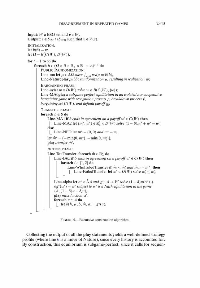
DISAGREEMENT IN REPEATED GAMES 2343
Input: W a BSG set and v ∈W .Output: s ∈ SIAC ∩ SNFD such that v ∈ V (s).
INITIALIZATION:let v(∅) = v;let Ω= B
(C(W )�D(W )
);
for t = 1 to ∞ doforeach h ∈ (Ω× B × R+ × R+ × A)t−1 do
PUBLIC RANDOMIZATION:Line-mu let μ ∈ �Ω solve
∫w∈Ω wdμ= v(h);
Line-Natureplay public randomization μ, resulting in realization w;
BARGAINING PHASE:Line-uylet w ∈ D(W ) solve w ∈ B(C(W )� {w});Line-MA0play a subgame perfect equilibrium in an isolated noncooperativebargaining game with recognition process ρ, breakdown process β,bargaining set C(W ), and default payoff w;
TRANSFER PHASE:foreach b ∈ B do
Line-MA1 if b ends in agreement on a payoff w′ ∈ C(W ) thenLine-MA2 let (m∗�w∗) ∈ R
20 ×D(W ) solve (1 − δ)m∗ +w∗ =w′;
elseLine-NFD let m∗ = (0�0) and w∗ =w;
let m∗ = (−min{0�m∗1}�−min{0�m∗
2});
play transfer m∗;
ACTION PHASE:Line-TestTransfer foreach m ∈ R
2+ do
Line-IAC if b ends in agreement on a payoff w′ ∈ C(W ) thenforeach i ∈ {1�2} do
Line-WhoFailedTransfer if mi < m∗i and m−i = m∗
−i thenLine-FailedTransfer let w∗ ∈ D(W ) solve w∗
i ≤w′i;
Line-alpha let α∗ ∈ �A and g∗ : A →W solve (1 − δ)u(α∗)+δg∗(α∗) = w∗ subject to α∗ is a Nash equilibrium in the game〈A� (1 − δ)u+ δg∗〉;play mixed action α∗;foreach a ∈ A do
let v(h�μ�b� m�a) = g∗(a);
FIGURE 5.—Recursive construction algorithm.
Collecting the output of all the play statements yields a well-defined strategyprofile (where line 6 is a move of Nature), since every history is accounted for.By construction, this equilibrium is subgame-perfect, since it calls for sequen-
2344 D. A. MILLER AND J. WATSON
tially rational actions in every bargaining phase (by Lemma 6), sequentiallyrational transfers in every transfer phase (by lines 10–13 and 16–20), and se-quentially rational mixed actions in every action phase (by line 21).
Axiom NFD is satisfied by line 13, which sets all disagreements to yield thesame disagreement payoff w. Axiom IAC is satisfied by lines 10–11 and 17–20,which ensure that any agreement payoff w′ ∈ C(W ) with w′ ∈ D(W ) is imple-mented. Therefore, if W is a BSG set and v ∈ W , the output is a strategy profiles ∈ SIAC ∩ SNFD. The equilibrium payoff is v ∈ V (s) by construction. Q.E.D.
LEMMA 8: If s ∈ SIAC ∩ SNFD, then coV (s) is a BSG set.
PROOF: Since s ∈ SNFD, every bargaining phase has a well-defined dis-agreement payoff. Since s ∈ SIAC, every proposal w ∈ C(coV (s)), if accepted,leads to continuation payoff w. Standard recursive techniques for character-izing equilibrium continuation values in bargaining games (for instance, re-lating the proposer’s supremum values in one round to the players’ supre-mum continuation values from the next round) establish that the bargainingphase has a unique equilibrium outcome and that it has the same represen-tation as in Lemma 6. Further, coV (s) must have a closed Pareto boundary;otherwise existence is violated in the bargaining phase. By sequential ratio-nality, the disagreement payoff w after any history satisfies w ∈ D(V (s)) ⊆D(coV (s)). Thus the equilibrium payoff from the bargaining phase is w ∈B(C(coV (s))�D(coV (s))), so every continuation value from the start of aperiod satisfies v ∈ coB(C(coV (s))�D(coV (s))). Hence coV (s) is a BSGset. Q.E.D.
For the following two lemmas, let W ∗ be the dominant BSG set.
LEMMA 9: Inputting W ∗ and any v ∈ W ∗ into the recursive construction algo-rithm of Figure 5 yields a strategy profile s∗ ∈ SPEAC such that v ∈ V (s∗).
PROOF: By definition, W ∗ fully Pareto dominates every BSG set. ByLemma 8, therefore, W ∗ fully Pareto dominates V (s) for every equilibriums ∈ SIAC ∩ SNFD. Since W ∗ is also a BSG set, every v ∈ W ∗ is available ineach bargaining phase. Since the recursive construction algorithm always pro-duces an equilibrium s ∈ SIAC ∩ SNFD, with input W ∗ it produces an equilibriums∗ ∈ SPEAC. Q.E.D.
LEMMA 10: If s∗ ∈ SPEAC, then V (s∗)⊆W ∗.
PROOF: By Lemma 8, coV (s∗) is a BSG set. By PEAC and Lemma 9, everypayoff in W ∗ is in the bargaining set of every bargaining phase. By sequentialrationality, therefore, no v ∈ V (s∗) can be strictly Pareto dominated by anyv′ ∈ W ∗. This implies that if W ∗ fully Pareto dominates V (s∗), then it must bethat V (s∗)⊆ W ∗. Finally, since W ∗ = coW ∗, we have coV (s∗)⊆W ∗. Q.E.D.
DISAGREEMENT IN REPEATED GAMES 2345
A.3. Existence and Construction
PROOF OF LEMMA 1: By construction of B, for any set W , the ele-ments of B(C(W )�D(W )) are on a line of slope −1, so coB(C(W )�D(W ))is a line segment of slope −1. That W ⊆ B(C(W )�D(W )) implies thatW ⊆ V (SSPE), wherein each v ∈ V (SSPE) is bounded above by v1 + v2 ≤maxα∈�A(u1(α)+u2(α)) and bounded below by vi ≥ minα−i∈�A−i
maxαi∈�Aiui(α)
for each i. Q.E.D.
The following lemma establishes some basic properties of B, C, and D. Else-where we take these properties for granted without reference to this lemma.
LEMMA 11: (i) W nonempty ⇒ D(W ) nonempty ⇒ C(W ) nonempty. (ii) Wcompact ⇒ D(W ) compact ⇒ C(W ) closed. (iii) P(W ) a nonempty line segmentof slope −1 and W nonempty with P(W ∪W ) = P(W ) ⇒ B(W �W ) nonempty;(iv) W also compact ⇒ B(W �W ) compact ⇒ coB(W �W ) compact.
The results in Lemma 11 follow from the definitions of B, C, and D, the factthat the Nash equilibrium correspondence is upper hemicontinuous, and thefact that every stage-game Nash equilibrium is enforced by a constant contin-uation value function.
PROOF OF LEMMA 2: Since W is a closed BSG set and z2 is the end-point that most favors player 1, z2
1 is the maximum payoff for player 1 thatcan be supported utilizing continuation values from W associated with thenext period, that is, z2
1 = max{v1|v ∈ B(C(W )�D(W ))}. Because elements inB(C(W )�D(W )) correspond to various disagreement points in D(W ), thismaximization problem can be expressed using the bargaining solution (Eq. (4)with C(W ) in place of W ), taking the disagreement point as the choice vari-able. Since level(W ) = maxw∈C(W )(w1 + w2) for any given disagreement pointw ∈D(W ), in bargaining, player 1 earns the value w1 +π1(level(W )−w1 −w2).Therefore,
z21 = max
w�g�α
(π2w1 −π1w2 +π1 level(W )
)(21)
s.t. w = (1 − δ)u(α)+ δg(α) and g : A → W enforces α
We next rewrite the optimization problem with a change of variables. Defineη(a) ≡ g1(a)− z2
1 for every a. Because the welfare level of every point in W islevel(W ), we have g2(a) = z2
2 −η(a). Also, the constraint that g(a) ∈ co{z1� z2}is equivalent to the requirement that η(a) ∈ [z1
1 − z21�0]. Using η to substitute
2346 D. A. MILLER AND J. WATSON
for g and w, and combining terms, we see that Eq. (21) is equivalent to
z21 = max
η�α
((1 − δ)
(π2u1(α)−π1u2(α)
)(22)
+ δ(π2z
21 −π1z
22
) + δη(α)+π1 level(W ))
s.t.
⎧⎨⎩η : A → [
z11 − z2
1�0]
extended to �A�
α ∈ �A is a Nash equilibriumof
⟨A� (1 − δ)u+ δ(η�−η)+ δz2
⟩
In the objective function on the right, we substitute for z22 using the equality
z21 + z2
2 = level(W ). Combining terms and moving the constant δz21 to the left
side yields
z21 = π1 level(W )+ max
η�α
(π2u1(α)−π1u2(α)+ δ
1 − δη(α)
)�(23)
subject to the conditions above. Recalling the definition of γ2, we have theconclusion of the lemma. Analyzing endpoint z1 in the same way gives thesimilar expression for z1
2 .The optimum defining γi exists for each i because the stage game is fi-
nite, the set of feasible η functions is compact, and the Nash correspon-dence is upper hemicontinuous. Regarding the final claim of the lemma, letαNE be a Nash equilibrium of the stage game. Note that αNE and η ≡ 0 sat-isfy the conditions of the maximization problems that define γ1 and γ2, soγ2(d) ≥ π2u1(α
NE) − π1u2(αNE) and γ1(d) ≥ π1u2(α
NE) − π2u1(αNE). Sum-
ming, we have that γ2(d)+ γ1(d)≥ 0. Q.E.D.
PROOF OF LEMMA 3: Let z1 and z2 denote the endpoints of W , and let z′1
and z′2 denote the endpoints of W ′. Suppose that span(W ) ≥ span(W ′). Thelarger span of W can support weakly more mixed actions in the stage gameas equilibria than W ′ can, because it provides a greater range of continua-tion values. This comparison does not depend on the location of the endpointsor the levels of the two sets (which are mere constants in the players’ pay-offs), only their relative spans. Thus any mixed action that can be supported byW ′ can also be supported by W , so level(W ) ≥ level(W ′). Furthermore, sinceeach γj(d) is increasing in d, Lemma 2 and the larger span of W imply thatzji ≥ z
′ji for each i �= j, which suffices to establish that W fully Pareto domi-
nates W ′. Q.E.D.
REFERENCES
ABREU, D., D. G. PEARCE, AND E. STACCHETTI (1990): “Toward a Theory of Discounted Re-peated Games With Imperfect Monitoring,” Econometrica, 58 (5), 1041–1063. [2305,2309]
DISAGREEMENT IN REPEATED GAMES 2347
(1993): “Renegotiation and Symmetry in Repeated Games,” Journal of Economic The-ory, 60, 217–240. [2321,2333,2335]
ARVAN, L., L. M. B. CABRAL, AND V. SANTOS (1999): “Meaningful Cheap Talk Must ImproveEquilibrium Payoffs,” Mathematical Social Sciences, 37 (1), 97–106. [2333]
ASHEIM, G. B. (1991): “Extending Renegotiation-Proofness to Infinite Horizon Games,” Gamesand Economic Behavior, 3 (3), 278–294. [2333,2334]
BAKER, G., R. GIBBONS, AND K. J. MURPHY (1994): “Subjective Performance Measures inOptimal Incentive Contracts,” Quarterly Journal of Economics, 109 (4), 1125–1156. [2306,
2328](2002): “Relational Contracts and the Theory of the Firm,” Quarterly Journal of Eco-
nomics, 117 (1), 39–84. [2306]BALIGA, S., AND R. EVANS (2000): “Renegotiation in Repeated Games With Side-Payments,”
Games and Economic Behavior, 33, 159–176. [2336]BERGIN, J., AND W. B. MACLEOD (1993): “Efficiency and Renegotiation in Repeated Games,”
Journal of Economic Theory, 61 (1), 42–73. [2333]BERNHEIM, B. D., AND D. RAY (1989): “Collective Dynamic Consistency in Repeated Games,”
Games and Economic Behavior, 1 (4), 295–326. [2307,2333,2336]BEUVE, J., AND S. SAUSSIER (2012): “Interfirm Cooperation in Strategic Relationships: The Role
of Formal Contract,” Industrial and Corporate Change, 21 (4), 811–836. [2329]BINMORE, K. (1987): “Perfect Equilibria in Bargaining Models,” in The Economics of Bargaining,
ed. by K. Binmore and P. Dasgupta. Oxford: Basil Blackwell, Chapter 5, 77–105. [2312]BLUME, A. (1994): “Intraplay Communication in Repeated Games,” Games and Economic Be-
havior, 6 (2), 181–211. [2335]BRANDENBURGER, A., AND H. STUART (2007): “Biform Games,” Management Science, 53 (4),
537–549. [2338]CHASSANG, S. (2010): “Building Routines: Learning, Cooperation, and the Dynamics of Incom-
plete Relational Contracts,” American Economic Review, 100 (1), 448–465. [2306]COOPER, D. J., AND K.-U. KÜHN (2013): “Communication Renegotiation, and the Scope for
Collusion,” American Economic Journal: Microeconomics (forthcoming). [2337]COOPER, R., D. V. DEJONG, R. FORSYTHE, AND T. W. ROSS (1989): “Communication in the
Battle of the Sexes Game: Some Experimental Results,” RAND Journal of Economics, 20 (4),568–587. [2337]
(1992): “Communication in Coordination Games,” Quarterly Journal of Economics, 107(2), 739–771. [2337]
CRAWFORD, V. (1998): “A Survey of Experiments on Communication via Cheap Talk,” Journal ofEconomic Theory, 78 (2), 286–298. [2337]
DEN HAAN, W. J., G. RAMEY, AND J. WATSON (2000): “Job Destruction and Propagation ofShocks,” American Economic Review, 90 (3), 482–498. [2331,2332]
(2003): “Liquidity Flows and Fragility of Business Enterprises,” Journal of MonetaryEconomics, 50, 1215–1241. [2331]
DIAMOND, P. A., AND E. S. MASKIN (1979): “An Equilibrium Analysis of Search and Breach ofContract, I: Steady States,” The Bell Journal of Economics, 10 (1), 282–316. [2331]
DOBBELAERE, S. (2004): “Estimation of Price-Cost Margins and Union Bargaining Power forBelgian Manufacturing,” International Journal of Industrial Organization, 22 (10), 1381–1398.[2332]
DOORNIK, K. (2006): “Relational Contracting in Partnerships,” Journal of Economics and Man-agement Strategy, 15 (2), 517–548. [2306]
FARRELL, J. (1987): “Cheap Talk, Coordination, and Entry,” RAND Journal of Economics, 18 (1),34–39. [2333]
(1988): “Communication, Coordination and Nash Equilibrium,” Economics Letters, 27(3), 209–214. [2333]
FARRELL, J., AND E. S. MASKIN (1989): “Renegotiation in Repeated Games,” Games and Eco-nomic Behavior, 1 (4), 327–360. [2307,2321,2333]
2348 D. A. MILLER AND J. WATSON
FONG, Y.-F., AND J. LI (2010): “Information Revelation in Relational Contracts,” Working Paper,available at http://goo.gl/BfmMm. [2306]
(2012): “Relational Contracts, Efficiency Wages, and Employment Dynamics,” WorkingPaper, available at http://goo.gl/0367r. [2306]
FONG, Y.-F., AND J. SURTI (2009): “The Optimal Degree of Cooperation in the Repeated Prison-ers’ Dilemma With Side Payments,” Games and Economic Behavior, 67 (1), 277–291. [2336]
FUCHS, W. (2007): “Contracting With Repeated Moral Hazard and Private Evaluations,” Ameri-can Economic Review, 97 (4), 1432–1448. [2306]
FUDENBERG, D., AND E. S. MASKIN (1986): “The Folk Theorem in Repeated Games With Dis-counting or With Incomplete Information,” Econometrica, 54 (3), 533–554. [2307]
GENICOT, G., AND D. RAY (2006): “Bargaining Power and Enforcement in Credit Markets,” Jour-nal of Development Economics, 79, 398–412. [2331]
GOLDLÜCKE, S., AND S. KRANZ (2012): “Infinitely Repeated Games With Public Monitoring andMonetary Transfers,” Journal of Economic Theory, 147 (3), 1191–1221. [2310]
(2013): “Renegotiation-Proof Relational Contracts,” Games and Economic Behavior,80, 157–178. [2321]
GROSSMAN, S., AND O. HART (1986): “The Costs and Benefits of Ownership: A Theory of Lateraland Vertical Integration,” Journal of Political Economy, 94, 691–719. [2338]
GUY, F. (2003): “High-Involvement Work Practices and Employee Bargaining Power,” EmployeeRelations, 25 (5), 455–471. [2332]
HALAC, M. (2012): “Relational Contracts and the Value of Relationships,” American EconomicReview, 102 (2), 750–779. [2306]
HALL, R. E., AND P. R. MILGROM (2008): “The Limited Influence of Unemployment on the WageBargain,” American Economic Review, 98 (4), 1653–1674. [2331]
HARRINGTON, JR., J. E. (1989): “Collusion Among Asymmetric Firms: The Case of DifferentDiscount Factors,” International Journal of Game Theory, 7 (2), 289–307. [2338]
HART, O., AND J. MOORE (1990): “Property Rights and the Nature of the Firm,” Journal of Polit-ical Economy, 98, 1119–1158. [2338]
HERMALIN, B. E., L. LI, AND T. NAUGHTON (2013): “The Relational Underpinnings of FormalContracting and the Welfare Consequences of Legal System Improvement,” Economics Letters,119 (1), 72–76. [2306]
JACKSON, M. O., AND T. R. PALFREY (1998): “Efficiency and Voluntary Implementation in Mar-kets With Repeated Pairwise Bargaining,” Econometrica, 66 (6), 1353–1388. [2306]
KLIMENKO, M., G. RAMEY, AND J. WATSON (2008): “Recurrent Trade Agreements and the Valueof External Enforcement,” Journal of International Economics, 74 (2), 475–499. [2306]
KVALØY, O., AND T. E. OLSEN (2006): “Team Incentives in Relational Employment Contracts,”Journal of Labor Economics, 24 (1), 139–169. [2306]
(2009): “Endogenous Verifiability and Relational Contracting,” American EconomicReview, 99 (5), 2193–2208. [2306,2329]
LAZZARINI, S. G., G. J. MILLER, AND T. R. ZENGER (2004): “Order With Some Law: Comple-mentarity versus Substitution of Formal and Informal Arrangements,” Journal of Law, Eco-nomics, and Organization, 20 (2), 261–298. [2329]
LEVIN, J. (2002): “Multilateral Contracting and the Employment Relationship,” Quarterly Journalof Economics, 117 (3), 1075–1103. [2306]
(2003): “Relational Incentive Contracts,” American Economic Review, 93 (3), 835–857.[2306,2321,2325,2327,2328,2332,2335]
MACLEOD, W. B., AND J. M. MALCOMSON (1989): “Implicit Contracts, Incentive Compatibility,and Involuntary Unemployment,” Econometrica, 57 (2), 447–480. [2306,2332]
(1998): “Motivation and Markets,” American Economic Review, 88 (3), 388–411. [2306,2332]
MILLER, D. A., AND J. WATSON (2013): “Supplement to ‘A Theory of Disagreement inRepeated Games With Bargaining’,” Econometrica Supplemental Material, 81, http://www.econometricsociety.org/ecta/supmat/10361_proofs.pdf. [2318]
DISAGREEMENT IN REPEATED GAMES 2349
MOEN, E. R., AND Å. ROSÉN (2011): “Incentives in Competitive Search Equilibrium,” Review ofEconomic Studies, 78 (2), 733–761. [2332]
MORTENSEN, D. T., AND C. A. PISSARIDES (1994): “Job Creation and Job Destruction in theTheory of Unemployment,” Review of Economic Studies, 61 (3), 397–415. [2331]
NASH, J. (1950): “The Bargaining Problem,” Econometrica, 18 (2), 155–162. [2315,2334]PEARCE, D. G. (1987): “Renegotiation-Proof Equilibria: Collective Rationality and Intertempo-
ral Cooperation,” Working Paper, available at http://goo.gl/2O585. [2307,2333]PEARCE, D. G., AND E. STACCHETTI (1998): “The Interaction of Implicit and Explicit Contracts
in Repeated Agency,” Games and Economic Behavior, 23, 75–96. [2306]RABIN, M. (1994): “A Model of Pre-Game Communication,” Journal of Economic Theory, 63 (2),
370–391. [2333]RADNER, R. (1985): “Repeated Principal-Agent Games With Discounting,” Econometrica, 53 (5),
1173–1198. [2306]RAFF, H., AND D. SCHMIDT (2000): “Cumbersome Coordination in Repeated Games,” Interna-
tional Journal of Game Theory, 29 (1), 101–118. [2306]RAMEY, V. (2011): “A Brief History of the Real Business Cycle—Search & Matching Literature,”
Manuscript, available at http://goo.gl/FOsA6. [2332]RAMEY, G., AND J. WATSON (1997): “Contractual Fragility, Job Destruction, and Business Cy-
cles,” Quarterly Journal of Economics, 112 (3), 873–911. [2306,2332](2001): “Bilateral Trade and Opportunism in a Matching Market,” Contributions to
Theoretical Economics, 1 (1). [2306,2332](2002): “Contractual Intermediaries,” Journal of Law, Economics, and Organization, 18
(2), 362–384. [2306,2338]RAY, D. (1994): “Internally Renegotiation-Proof Equilibrium Sets: Limit Behavior With Low
Discounting,” Games and Economic Behavior, 6 (1), 162–177. [2333]RAYO, L. (2007): “Relational Incentives and Moral Hazard in Teams,” Review of Economic Stud-
ies, 74 (3), 937–963. [2306]ROGERSON, R., R. SHIMER, AND R. WRIGHT (2005): “Search-Theoretic Models of the Labor
Market: A Survey,” Journal of Economic Literature, 43 (4), 959–988. [2332]RUBINSTEIN, A. (1980): “Strong Perfect Equilibrium in Supergames,” International Journal of
Game Theory, 9, 1–12. [2307,2321](1982): “Perfect Equilibrium in a Bargaining Model,” Econometrica, 50 (1), 97–109.
[2312]RYALL, M. D., AND R. C. SAMPSON (2009): “Formal Contracts in the Presence of Relational
Enforcement Mechanisms: Evidence From Technology Development Projects,” ManagementScience, 55 (6), 906–925. [2329]
SANTOS, V. (2000): “Alternating-Announcements Cheap Talk,” Journal of Economic Behavior &Organization, 42 (3), 405–416. [2333]
SCHMIDT, K. M., AND M. SCHNITZER (1995): “The Interaction of Explicit and Implicit Con-tracts,” Economics Letters, 48 (2), 193–199. [2306,2337,2338]
SHAKED, A., AND J. SUTTON (1984): “Involuntary Unemployment as a Perfect Equilibrium in aBargaining Model,” Econometrica, 52 (6), 1351–1364. [2312,2342]
SHAPIRO, C., AND J. E. STIGLITZ (1984): “Equilibrium Unemployment as a Worker DisciplineDevice,” American Economic Review, 74 (3), 433–444. [2332]
SLOOF, R., AND J. SONNEMANS (2011): “The Interaction Between Explicit and Relational Incen-tives: An Experiment,” Games and Economic Behavior, 73 (2), 573–594. [2337]
THOMAS, J., AND T. WORRALL (1988): “Self-Enforcing Wage Contracts,” Review of EconomicStudies, 55 (4), 541–553. [2306]
WATSON, J. (1991): “Communication and Superior Cooperation in Two-Player Normal FormGames,” Economics Letters, 35 (3), 267–271. [2333]
(2006): “Contract Game Theory: Basic Concepts for Settings With Finite Horizons,”Working Paper, available at http://goo.gl/NFtle. [2333]
2350 D. A. MILLER AND J. WATSON
Dept. of Economics, University of Michigan, 611 Tappan St., Ann Arbor, MI48109, U.S.A.; [email protected]
andDept. of Economics, University of California, San Diego, 9500 Gilman Dr., La
Jolla, CA 92093-0508, U.S.A.; [email protected].
Manuscript received October, 2011; final revision received March, 2013.