A Theory of Just-in-Time and the Growth in

Manufacturing Trade∗

John T. Dalton†

Wake Forest University

First Version: May 2009This Version: January 2013

Abstract

This paper argues the widespread adoption of Just-in-Time (JIT) logistics provides akey to understanding the growth in the U.S. trade share. To do so, I develop a dynamictrade model based on the choice of the logistics technology used in a firm’s supply chain.The model’s predicted trade dynamics depend on how the set of firms using JIT withinternational suppliers changes over time. A numerical example shows the model is capableof generating growth in the trade share. I present evidence showing the theory is consistentwith aggregate data as well as industry-level panel data.

JEL Classification: F10, F14, L60, M11Keywords: trade growth, Just-in-Time, newsvendor problem, airplane transportation

∗Previous versions of this paper circulated under the title “Explaining the Growth in Manufacturing Trade.”I am grateful to Tim Kehoe, Fabrizio Perri, and Cristina Arellano for their support and advice. I thank CostasArkolakis, Turkmen Goksel, Nick Guo, Tommy Leung, Jim Schmitz, Anderson Schneider, Mike Waugh, KevinWiseman, Hakki Yazici, and the members of the Trade and Development workshop at the University of Minnesotafor their suggestions and comments. I also thank participants of the XIV Workshop on Dynamic Macroeconomicsand the Humane Studies Research Colloquium for their many useful suggestions and comments, as well as seminarparticipants at the Federal Reserve Bank of Minneapolis, Boston College, the University of North Carolinaat Chapel Hill, North Carolina State University, Elon University, the Kiel Institute for the World Economy,Washington and Lee University, Wesleyan University, Wake Forest University, The University of the South, theUniversity of Bonn, the University of Georgia, the 2010 Midwest Macroeconomics Meetings, the 2010 MidwestInternational Trade Meetings, and the 2011 Eastern Economic Association Meetings. Financial support fromthe Graduate Research Partnership Program at the University of Minnesota and the Humane Studies Fellowshipand the Hayek Fund for Scholars from the Institute for Humane Studies is gratefully acknowledged.

†Contact: Department of Economics, Carswell Hall, Wake Forest University, Box 7505, Winston-Salem, NC27109. Email: daltonjt@wfu.edu.

1 Introduction

Since the end of World War II, during the so-called second era of globalization, a major change

in the U.S. economy has been the overall growth of manufacturing trade.1 Moreover, the growth

exhibits two phases, one before and one after the early 1980’s. Trade grows slower before the

early 1980’s than afterwards. These phenomena are largely considered the products of global

tariff reductions introduced by successive rounds of multilateral trade negotiations under the

umbrella of the General Agreement on Tariffs and Trade.

Yet, as discussed in Yi (2003), the tariff explanation poses a puzzle for standard trade models.

The observed decreases in tariffs are simply not large enough to generate the growth in trade.

In addition, tariff declines are larger before the early 1980’s than after, leaving standard models

unable to explain the acceleration in trade growth.2

This paper provides both new data evidence and a new theory to reconcile the manufacturing

trade growth puzzle. The explanation relies not on changes in tariff policy but on a fundamental

change in the organization of U.S. manufacturing—the adoption of Just-in-Time (JIT) logistics

in the early 1980’s.3 JIT is a system of manufacturing logistics in which materials or parts are

ordered and delivered just before they are needed in the production process. As a result, JIT

manufacturers gain flexibility in their ordering decisions, reduce the stocks of inventory held

on-site, and eliminate inventory carrying costs. The flexibility of JIT allows manufacturers to

meet all fluctuations in the demand for their products, which allows them to sell more than

if constrained by stocks of inventory. The savings generated by reducing inventory carrying

costs allow JIT manufacturers to charge lower prices for their products, which lead consumers

to increase demand. When firms engaged in international trade adopt JIT, both of these forces,

flexibility and the reduction of inventory carrying cost, generate increased trade volumes. Of

1The first era of globalization, on the other hand, refers to the decades leading up to World War I, commonlydated 1870-1913. See Estevadeordal, Frantz, and Taylor (2003) for work studying the growth of trade during thisperiod plus the subsequent collapse of trade during the years 1914-1939. Not all historians agree, however, withthis taxonomy of globalization. See O’Rourke and Williamson (2002) for a useful summary of the competingviews and an argument in favor of the nineteenth century as the beginning of globalization.

2See also Bergoeing and Kehoe (2003) and Bergoeing, Kehoe, Strauss-Kahn, and Yi (2004) for further workon the inability of standard models to generate the observed increase in trade.

3JIT also goes by the terms lean manufacturing or Toyota Production System, as JIT is primarily basedon production and logistics techniques developed and refined by Toyota. Ohno (1988) serves as the classicexplication of the Toyota Production System.

1

course, global supply chains incorporating JIT require airplane transportation for speedy delivery

of parts. Indeed, the rise of airplane transportation is an important characteristic of the second

era of globalization and is essential for understanding the growth of manufacturing trade in the

U.S.4 This is true for not only understanding the growth in trade due to the adoption of JIT for

those firms already engaged in international trade but also for the growth in trade due to firms

switching from using JIT with domestic suppliers to using JIT with international suppliers.

For example, if airplane transportation costs are prohibitively high, then a domestic firm in

the U.S. might choose to incorporate JIT in a domestic supply chain, foregoing potential gains

from trade since the speedy delivery of parts is so costly from international suppliers. Once

airplane transportation costs fall, however, the domestic firm might find it beneficial to conduct

JIT with an international supplier. This switching phenomenon leads to an immediate boost in

trade volumes.

At the firm level, Feinberg and Keane (2006) and Keane and Feinberg (2007) find reducing

inventories, a measure of JIT adoption, explains much of the growth in intra-firm trade between

a set of U.S. multinational corporations and their Canadian affiliates over the period 1983-1996.

At the aggregate level, the empirical strength of the JIT explanation lies both in the timing

and the magnitude of the adoption. First, the introduction of JIT logistics coincides with the

increased trade growth in the early 1980’s. Second, JIT spreads throughout the manufacturing

sector and, thus, has the potential to have a large impact on aggregate variables, such as total

trade.

In order to analyze the relation between JIT and the manufacturing trade growth puzzle, I

develop a dynamic model of international trade based on firms, their suppliers, and the logistics

technology used in their supply chains. In the model, without JIT, a domestic final good firm

faces a version of the newsboy or newsvendor problem, a classic model from the operations

research literature.5 In the version of the newsvendor problem used in the model, a firm chooses

both an inventory level and a selling price before uncertain final demand is realized. The firm’s

inventory consists of intermediate goods, either domestically or internationally supplied, used

for final good production, and the price is that faced by consumers of the firm’s final good.

4See Hummels (2001), Hummels (2007), Hummels and Schaur (2010), and Harrigan (2010) for examples ofthe role of airplanes in facilitating international trade.

5See Petruzzi and Dada (1999) for an overview of the newsvendor problem.

2

Inventories constrain a firm’s ability to respond to fluctuations in demand. In addition, the

price set by a firm reflects not only the marginal cost of production but also the additional

costs associated with maintaining inventories in an uncertain world. As a result, the price set

by a firm facing the newsvendor problem is higher than that set in an environment without

such constraints. The higher price results in lower final demand. Once a firm adopts JIT in

the model, however, it does not face the newsvendor problem. The firm can now respond to

all fluctuations in final demand and set a lower selling price. These two effects, which I refer

to as the flexibility and price effects, lead to increased sales and, in the case of a firm using an

international supplier, increased trade volumes. In the case of a firm using a domestic supplier

and also already having adopted JIT, if the firm switches to using JIT with an international

supplier, then the switching leads to increased trade volumes. I refer to this as the switching

effect. A firm’s choice of logistics technology and supplier determines the potential trade flow

generated by a firm. When and how the logistics and supplier choice occurs then impacts the

dynamics of trade.

When using an international supplier, the logistics technology implies a transportation mode

used in a firm’s global supply chain. Without JIT, a firm orders parts and has them delivered

by ocean shipping. JIT, however, requires the speedy delivery of parts. A firm using JIT uses

airplane transportation to deliver its foreign intermediates. Air shipping costs more than ocean

shipping, though, and the size of a firm’s ad valorem air freight wedge determines whether the

firm adopts JIT logistics. I introduce multiple final good firms, group firms by industry, and

differentiate industries by the final good’s value-to-weight ratio. The ad valorem air freight

wedge decreases in the value-to-weight ratio. Firms in industries with a higher ad valorem air

freight wedge are less likely to adopt JIT. The number of firms using each logistics technology

determines the potential aggregate trade volume.

How the number of JIT firms with international suppliers changes over time, driven in part

by changes in the cost of air transportation, determines the dynamics of aggregate trade flows.6

A numerical example illustrates the mechanics of the model and shows the model is capable of

capturing part of the growth in trade beginning in the early 1980’s.

Although the central focus of this paper is to explain the growth in manufacturing trade,

6I say “in part” because I also introduce a cost of adopting JIT in the model.

3

my theoretical framework provides a number of additional testable implications which I explore.

Since the dynamics of aggregate trade flows are driven by those firms using international sup-

pliers adopting JIT in the model, the model predicts the timing of the changes in these trade

flows should coincide with changes to other model statistics generated purely from the adoption

of JIT. For instance, the model’s implied aggregate inventory-to-sales ratio decreases with the

adoption of JIT, and the aggregate value of goods traded via airplane transportation increases.

Both of these facts are reflected in the data. More importantly, the timing of both of these facts

coincides with the timing of the growth of manufacturing trade. The aggregate statistics from

the model result from summing across firms in different industries, which means the theory also

makes predictions for a cross-section of industries. Those industries with firms adopting JIT

should experience increased trade, decreased inventory-to-sales ratios, and increased value of

goods traded via airplanes. The paper presents evidence showing these cross-sectional implica-

tions appear in the data.

This paper brings three strands of literature together to study the manufacturing trade

growth puzzle. The first concerns itself directly with the question of how and why manufacturing

trade increased. Bergoeing and Kehoe (2003), Bergoeing, Kehoe, Strauss-Kahn, and Yi (2004),

and Yi (2003) show the inability of a number of standard trade models to account for the

rise in manufacturing trade. Yi (2003) specifically documents the inconsistency of a standard

explanation based solely on the observed decrease in tariffs. A number of papers have since

attempted to explain the growth in trade, including Alessandria and Choi (2008), Bajona (2004),

Bridgman (2008), Bridgman (2012) and Cunat and Maffezzoli (2007). However, this paper is

the first to take seriously the role played by the widespread adoption of JIT on the growth

of aggregate U.S. trade. In doing so, I draw on a second and third strand of literature. The

second is recent work highlighting the growing importance in international trade of airplane

transportation, which is essential for global supply chains incorporating JIT logistics. Hummels

(2007) documents the relation between the decline in airplane transportation costs and the value

of U.S. exports and imports shipped internationally by airplane.7 Hummels (2001) looks closer

at the role of shipment time as a barrier to trade and quantifies the decreased shipment time

due to airplanes in tariff equivalent terms. Harrigan (2010) builds on these facts by developing

7See Hayakawa (2010) for evidence linking airplane transportation and trade shipments for the case of Japan.

4

a simple model of Ricardian comparative advantage in which airplanes play a leading role.

The third strand of literature related to this paper is the operations research literature. The

newsvendor problem serves as the core for numerous applications in operations research. Many

references exist for these applications, but I simply refer to Petruzzi and Dada (1999), as it

provides a useful overview of the subject.

I organize the remainder of the paper as follows: Section 2 gives a brief overview of the

data regularities connecting JIT and airplane transportation with the growth of aggregate U.S.

manufacturing trade. In section 3, I develop the model used to explain the growth of trade.

Section 4 presents a numerical example. Section 5 examines panel data for evidence supporting

the model’s industry-level implications. Section 6 concludes.

2 Empirical Evidence

This section documents three facts about U.S. manufacturing central to the main idea of this

paper. I then provide an intuitive way of interpreting and tying these facts together which serves

as the basis for the theoretical framework developed in the subsequent section.

2.1 Three Facts About U.S. Manufacturing

The three facts concern the growth of trade, the decline in inventory, and the use of airplane

transportation. Figures (1) - (3) present data related to each of these facts.

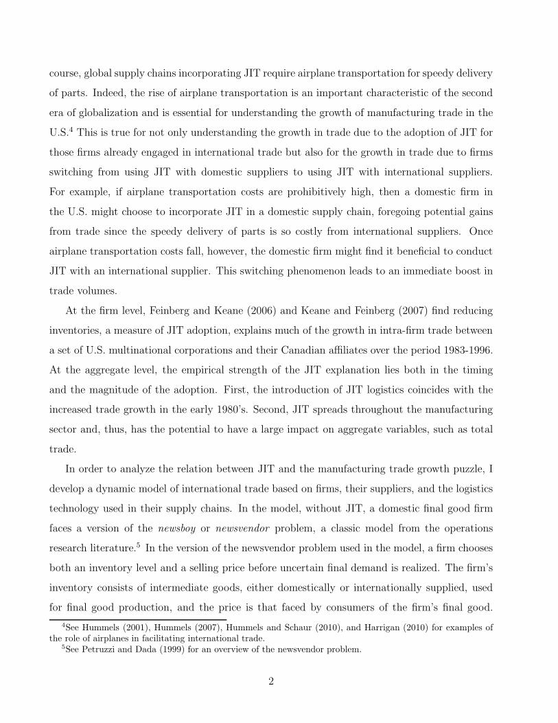
Figure (1) shows the growth in U.S. trade over the period 1970-2005, as measured by the

trade share of gross output in manufacturing. The manufacturing trade series is from the

Organisation for Economic Co-operation and Development’s (OECD) ITCS International Trade

by Commodity Database and is constructed by summing together the total value of imports

and exports in categories 5-8 of the SITC Revision 2 classification system.8 The data for

manufacturing gross output are from the OECD’s STAN Structural Analysis Database and the

Bureau of Economic Analysis’s Industry Economic Accounts. Two features of the data in figure

(1) bear mentioning, one quantitative, the other qualitative. First, the trade share of gross

8The categories are as follows: 5 Chemicals and related products, n.e.s.; 6 Manufactured goods classifiedchiefly by material; 7 Machinery and transport equipment; and 8 Miscellaneous manufactured articles.

5

0.00

0.10

0.20

0.30

0.40

0.50

1970 1975 1980 1985 1990 1995 2000 2005

Sh

are

Figure 1:Trade / Gross Output in U.S. Manufacturing

output in manufacturing increases by a factor of 4.70, from 0.09 in 1970 to 0.41 in 2005. From

the perspective of international trade, the overall quantitative increase in the data seems to

justify talk concerning a second era of globalization. Second, two phases exist in the series of

the trade share, one before and one after the early 1980’s. Specifically, the trade share grows

at an average rate of 4.24% over the years 1970-1983 and then accelerates to an average rate of

4.81% from 1984 to 2005.

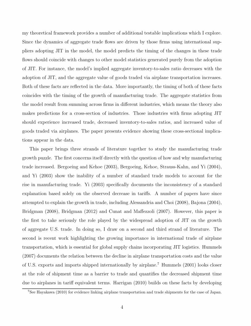
The series presented in figure (2) represents the inventory-to-sales ratio in U.S. manufactur-

ing over nearly half a century. These data are constructed from the NBER-CES Manufacturing

Industry Database and the U.S. Census Bureau’s Manufacturers’ Shipments, Inventories, and

Orders. The inventory-to-sales ratio is measured as the total value of inventories divided by

the total value of shipments in U.S. manufacturing. The overall trend is straightforward. The

inventory-to-sales ratio fluctuates within a band until the early 1980’s, at which point it begins

a steady decline. Over the period 1958-1983, the average inventory-to-sales ratio in U.S. man-

ufacturing is 0.15. By 2005, the inventory-to-sales ratio reaches 0.09, 37.58% smaller than the

6

0.08

0.09

0.10

0.11

0.12

0.13

0.14

0.15

0.16

0.17

1958 1964 1970 1976 1982 1988 1994 2000

Sh

are

2005

Figure 2:Inventory / Sales in U.S. Manufacturing

average before 1983. The large fluctuations in figure (2) correspond to business cycles. Some

authors refer to the period after the early 1980’s, during which the fluctuations appear less

pronounced, as the Great Moderation.9

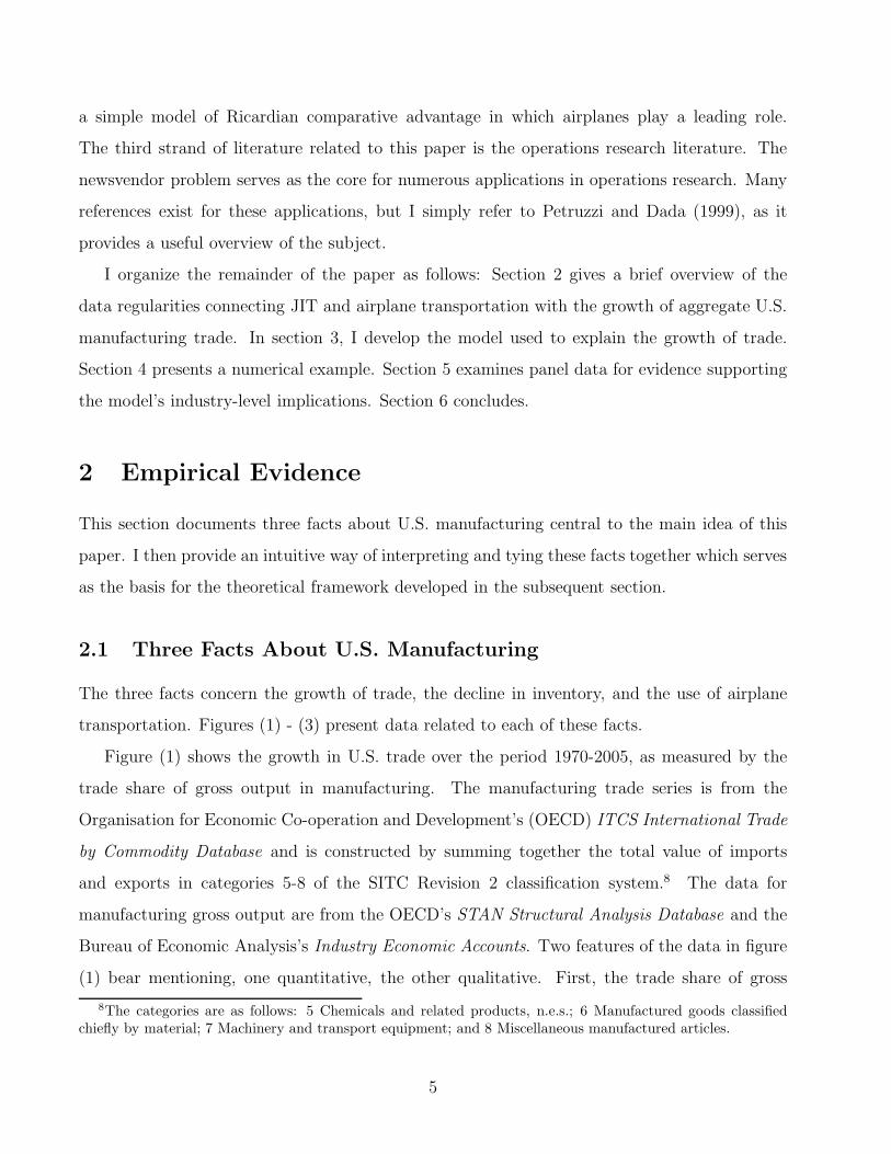
Figure (3) documents the growing importance of airplane transportation as a means of

trading goods internationally. Although it is true the total tonnage of traded goods shipped on

airplanes is negligible when compared to that shipped on boats, airplanes do play a significant

role in terms of the total value of goods traded.10 The data in figure (3) document this fact for

the case of U.S. manufacturing imports. The figure displays the total value of manufacturing

imports shipped by airplanes as a share of the total value of all manufacturing imports, which I

construct from the database used in Hummels (2007). The database is originally based on the

9There is an ongoing body of research surrounding the Great Moderation. For an overview, see Bernanke(2004), Blanchard and Simon (2001), McConnell and Perez-Quiros (2000), and Stock and Watson (2003). SeeDavis and Kahn (2008) and Kahn, McConnell, and Perez-Quiros (2002) for the view that the adoption of betterinventory management techniques, like JIT logistics, led to the decline in macroeconomic volatility experiencedduring the Great Moderation.

10See Hummels (2007) for a thorough discussion on shipping and international trade during the period 1950-2005.

7

0.00

0.05

0.10

0.15

0.20

0.25

0.30

0.35

0.40

1970 1975 1980 1985 1990 1995 2000

Sh

are

2004

Figure 3:Total Air Imports / Total Imports (Less C&M) in U.S. Manufacturing

U.S. Census Bureau’s U.S. Imports of Merchandise. Again, I define manufacturing as categories

5-8 of SITC Revision 2, the classification system used in the database from Hummels (2007). I

also remove the trade flows from Canada and Mexico, since most of these shipments arrive by

truck or rail.11 The air share of manufacturing imports increases from 0.12 in 1970 to 0.32 in

2004, a factor of 2.68. As with the data in figures (1) and (2), the onset of the 1980’s signals a

change, and the air share enters a period of sustained increase.

2.2 Tying the Facts Together

Figures (1) - (3) document that the onset of the growth in the trade share in the early 1980’s

coincides with both the decline in the inventory-to-sales ratio and the increased use of air-

planes to import goods from abroad. The adoption of JIT logistics in the early 1980’s by U.S.

manufacturing firms provides the key to tying these three facts together.

11And, since most shipments arrive by truck or rail, removing Canada and Mexico from the data does notchange the qualitative features in figure (3); the series is simply “shifted down,” as each year’s air share is reducedin size.

8

Broadly defined, JIT is a system of manufacturing logistics in which materials or parts are

ordered and delivered just before they are needed. Both the ordering and delivery components

of this definition are essential for a well-functioning JIT system. Being able to order materials

or parts just before they are needed requires a firm to process and convey production orders

through a communication system to various units within the firm or suppliers outside the firm.

This communication system need not be composed of computers, internet connections, and

logistics software, though these have been widely used over the past several decades. Toyota,

for instance, developed the kanban system, which was a series of posted placards used to trigger

certain tasks within the firm. The other essential component of JIT is the speedy delivery of

materials or parts once they are ordered. A firm using JIT requires its suppliers to make frequent

and fast deliveries depending on the needs of the firm.

One of the main goals of JIT is to eliminate all inventories in the production process, as

inventories are viewed as a source of waste and inefficiency. Achieving this goal provides two

key benefits. First, eliminating inventories requires a firm to maintain its ordering and delivery

system to meet production orders, which means a firm attains a high degree of flexibility in

its operations. In an uncertain selling environment, flexibility allows a firm to respond to all

fluctuations in the demand for its product without being constrained by inventories. Second,

eliminating inventories results in an obvious reduction in a firm’s inventory carrying costs. A

firm does not have to pay for warehouse space to store its inventory, for example. Reduced

inventory carrying costs allow a firm to charge lower prices for its product, thereby increasing

demand. Note these two benefits occur along a type of extensive and intensive margin for a

firm, both of which can lead to greater sales compared to when not using JIT.

So, why did U.S. manufacturing firms not adopt JIT techniques before the early 1980’s?

After all, JIT was in widespread use in Japan throughout the 1970’s. Keane and Feinberg

(2007) argues U.S. firms were simply not tuned in to the benefits of JIT until after Japanese

firms began to capture market share across a wide range of industries in the late 1970’s and

early 1980’s. Large U.S. firms, like General Electric, began to send study teams to Japan to

investigate why Japanese firms were outperforming their American competitors. Only then did

U.S. manufacturing firms discover the use of JIT. As a result, large U.S. manufacturing firms

gradually adopted JIT and, as discussed in Keane and Feinberg (2007), later marketed software

9

packages designed to implement JIT, which facilitated the adoption of JIT throughout U.S.

manufacturing.12

This widespread adoption of JIT ties together figures (1) - (3). Beginning in 1983, a struc-

tural break occurs in the inventory-to-sales ratio, initiating a steady decline thereafter (figure

(2)).13 For those manufacturing firms with global supply chains, adopting JIT requires the use of

airplane transportation, since the speedy delivery of parts is a crucial element of the system (fig-

ure (3)). Otherwise, firms would be adopting JIAM, Just-in-a-Month, as ocean transportation

imposes considerable time costs.14 The cost of airplane transportation serves as an additional

cost of adopting JIT for those firms relying on global supply chains.15 These firms contribute

to the acceleration in the growth of trade after 1983 through increased sales resulting from the

two main benefits of JIT, its flexibility and price effects (figure (1)). For some of those manu-

facturing firms initially adopting JIT with domestic suppliers, the continual decline in airplane

transportation costs eventually creates opportunities to adopt JIT with international suppliers.

This switching effect contributes to the growth of trade after 1983. The theoretical framework

developed in section 3 formalizes this interpretation of figures (1) - (3).

3 Model

In this section, I describe a dynamic model of international trade whose core component is the

logistics technology used in a firm’s supply chain. The economy consists of a home country, say

the U.S., and the rest of the world. Within the home country, final good firms use intermediate

goods to produce output for domestic consumption. Final good firms purchase intermediates

either from a domestic supplier in the home country or a foreign supplier in the rest of the world.

Final good firms also choose a logistics technology, either Non-JIT or JIT, to use in their supply

chains. A firm’s choice of supplier and logistics technology depends on firm-specific character-

12I interpret this historical evidence to suggest technological improvements led to a decline in the cost ofadopting JIT. Later, in the context of my model, I capture these technological improvements in the form of adecreasing fixed cost of adopting JIT.

13The 1983 break motivates me to base the discussion of figures (1) - (3) in section 2.1 on the two periods1970-1983 and 1984-2005. Feinberg and Keane (2006), Kahn, McConnell, and Perez-Quiros (2002), and Keaneand Feinberg (2007) also discuss the structural break in the U.S. manufacturing inventory-to-sales ratio.

14Hummels (2001) notes shipping containers from Europe to parts of the U.S. can require two to three weeks,while those from East Asia can take as much as six weeks.

15The evolution of airplane transportation costs plays a prominent role in the theory developed in section 3.

10

istics and a fixed cost of using JIT. The firm-specific characteristics include air transportation

costs and ideal supplier matches, which I explain in detail below. The sorting of final good firms

into supplier and logistics technology choices gives rise to aggregate statistics for the economy.

Exogenous changes in the air transportation costs and the fixed cost of using JIT determine

how the sorting of final good firms changes over time and, thus, how the aggregate statistics in

the economy evolve.

I begin developing the model by first describing the demand for final goods and the produc-

tion and logistics technologies used to produce them. Next, I analyze two stationary equilibria

in which the fixed cost of using JIT and the air transportation costs do not change over time. As

a result, a final good firm never switches its logistics technology. The two stationary equilibria

I examine are the cases when a final good firm only uses the Non-JIT or JIT technology. This

stationary analysis allows me to highlight the differences between an economy populated by

Non-JIT firms versus an economy populated by JIT firms. I then discuss the transition from

using the Non-JIT technology to using the JIT technology.

3.1 Demand

Consider a home country firm selling a final good q in its domestic market.16 A firm’s final good

faces uncertain demand D(p, ε) specified as follows:

D(p, ε) = y(p)ε, where y(p) = ap−b. (1)

y(p) governs the shape of the demand curve faced by a firm, where a > 0 and b > 1, and p is

the price of the final good set by a firm. ε determines the size of the market, where ε ∈ [ε, ε],

ε > 0, E(ε) = 1, and ε is i.i.d. over time.17 I refer to the c.d.f. of ε as F (·).

3.2 Production and Logistics

A home country firm produces the final good q from either domestically or internationally

supplied intermediate goods, denoted md and mf , respectively. If a home country firm uses

16I suppress time subscripts since the problem appears below written recursively.17Below, I introduce multiple firms into the model, each of which faces its own demand. ε is i.i.d. across these

firms.

11

domestic intermediates, it produces q with the following production technology:

q =md

cd, (2)

where cd is a random inverse productivity term drawn from an exponential distribution and

specific to a home country final good firm. cd remains fixed over time and governs the effi-

ciency with which a final good firm is able to transform domestic intermediates into final goods.

Similarly, if a home country firm uses foreign intermediates, it produces final good q with the

production technology

q =mf

cf. (3)

Again, cf remains fixed over time and governs the efficiency with which a final good firm trans-

forms international intermediates into final goods. Instead of drawing cf from an exponential

distribution, however, I simply normalize the efficiency of international intermediates by setting

cf = 1.

The relation between cd and cf gives rise to what I refer to as a final good firm’s ideal

supplier, which drives the desire to trade in the model. cd and cf are analogous to unit labor

costs, and, thus, the trade structure in my model has a Ricardian flavor. If cd > 1, then a final

good firm’s ideal supplier is international. If cd < 1, then a final good firm’s ideal supplier is

domestic. A final good firm’s ideal supplier is either domestic or international when cd = 1.

A home country firm producing final goods chooses the type of logistics technology used in

its supply chain, either a Non-JIT or JIT logistics technology. The following characteristics

define the logistics technologies:

Non-JIT :

1) Decisions regarding final good q must be made before uncertainty is realized.

2) Inventory facilities exist to store q.

3) Ocean or domestic shipping is used to transport q depending on the location of the

intermediate good supplier.

JIT :

1) Final good q is ordered after uncertainty is realized.

12

2) No inventory facilities exist to store q.

3) Air or domestic shipping is used to transport q depending on the location of the

intermediate good supplier.

4) Operating JIT requires a per period fixed cost f .

The differences between operating the Non-JIT and JIT technologies appear explicitly when

writing down the final good firm’s maximization problem in the subsequent sections. Note the

assumption of either ocean or air shipping when using an international supplier implies a stylized

geography. The home country is an “island” which imports goods from abroad. Whether a final

good firm decides to operate JIT depends on the fixed cost, in the case of using a domestic

supplier, or the fixed cost and a firm-specific ad valorem air freight charge τ , in the case of using

an international supplier. The fixed cost relates to the ordering component of JIT discussed in

section 2.2 and is meant to capture those costs associated with implementing and maintaining

the communications system in a JIT supply chain. Similarly, the air freight charge relates

to the delivery component, as a firm using JIT with an international supplier requires speedy

transportation.

The preceding discussion refers to a single final good firm in the home country with an

associated cd and τ , but I consider an economy with multiple firms throughout the rest of

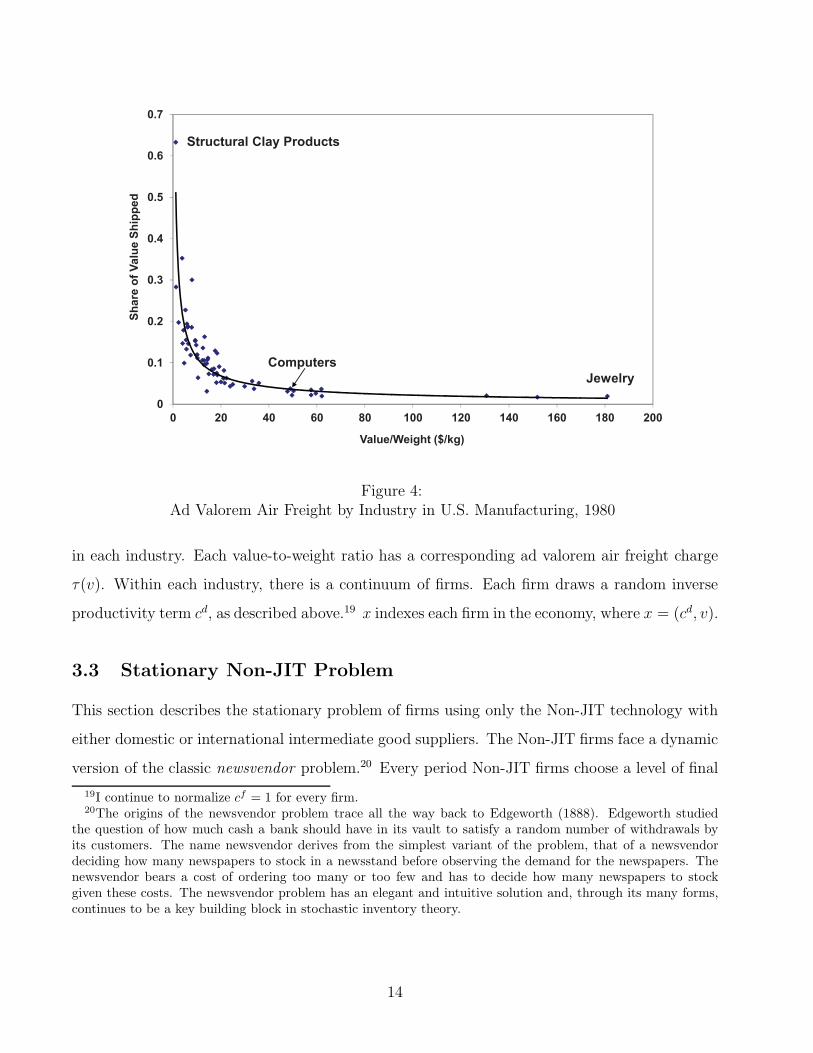
this paper. Figure (4) motivates the setup of firms in the model. The data in figure (4)

document the relation between a manufacturing good’s value-to-weight ratio and the associated

ad valorem air freight charge for the sample year 1980.18 I use the U.S. manufacturing import

data from Hummels (2007) to construct figure (4). I filter the data through a concordance

to construct 66 industries corresponding to 66 3-digit SIC manufacturing industries. Dividing

the total value of manufacturing imports shipped by airplanes by the total weight of those

same imports generates a value-to-weight ratio for each industry. Likewise, dividing the total

value of the shipping charges paid on the manufacturing imports shipped by airplanes by the

total value of those same imports results in an ad valorem air freight charge for each industry.

Figure (4) shows that as an industry’s value-to-weight ratio increases the ad valorem air freight

charge decreases. Returning to the model, the home country contains a continuum of industries

indexed by v ∈ [0, 1]. Industries differ by the value-to-weight ratio of the final goods produced

18The choice of 1980 is arbitrary, as the relation in figure (4) holds for other years in the data as well.

13

0

0.1

0.2

0.3

0.4

0.5

0.6

0.7

0 20 40 60 80 100 120 140 160 180 200

Sh

are

of

Valu

e S

hip

ped

Value/Weight ($/kg)

JewelryComputers

Structural Clay Products

Figure 4:Ad Valorem Air Freight by Industry in U.S. Manufacturing, 1980

in each industry. Each value-to-weight ratio has a corresponding ad valorem air freight charge

τ(v). Within each industry, there is a continuum of firms. Each firm draws a random inverse

productivity term cd, as described above.19 x indexes each firm in the economy, where x = (cd, v).

3.3 Stationary Non-JIT Problem

This section describes the stationary problem of firms using only the Non-JIT technology with

either domestic or international intermediate good suppliers. The Non-JIT firms face a dynamic

version of the classic newsvendor problem.20 Every period Non-JIT firms choose a level of final

19I continue to normalize cf = 1 for every firm.20The origins of the newsvendor problem trace all the way back to Edgeworth (1888). Edgeworth studied

the question of how much cash a bank should have in its vault to satisfy a random number of withdrawals byits customers. The name newsvendor derives from the simplest variant of the problem, that of a newsvendordeciding how many newspapers to stock in a newsstand before observing the demand for the newspapers. Thenewsvendor bears a cost of ordering too many or too few and has to decide how many newspapers to stockgiven these costs. The newsvendor problem has an elegant and intuitive solution and, through its many forms,continues to be a key building block in stochastic inventory theory.

14

good output q and a selling price pN .21 The level of output consists of any inventories of final

goods on hand s and new production of final goods q−s. Non-JIT firms make decisions regarding

q and pN before demand uncertainty is realized, that is, based on expected discounted profits.

After the uncertainty is realized, Non-JIT firms inventory any remaining output q − D(pN , ε)

for use in the next period.

The Non-JIT firm problem using either a domestic or an international supplier can be written

as follows:

V iN(s; x) = max

pN ,q≥0

∫ q

y(pN )

ε

[

pND(pN , ε)− pmci[q − s]− pI [q −D(pN , ε)] + βV i

N(s′; x)

]

dF (ε)

+

∫ ε

q

y(pN )

[

pNq − pmci[q − s] + βV i

N(s′; x)

]

dF (ε) (4)

s.t. s′ =

q −D(pN , ε), for D(pN , ε) ≤ q

0, for D(pN , ε) > q,(5)

where i = d, f and 0 < β < 1. pm and pI are the prices for ordering and inventorying an extra

unit of good q. Problem (4) is written so that the production function (2) or (3) is already

embedded within the objective function. If the firm produces q − s new units of the final good,

then it orders ci[q − s] units of the intermediate good, i = d, f . The first half of equation (4)

represents the expectation with respect to the distribution of demand shocks over the profit

region when D(pN , ε) ≤ q. In this region, D(pN , ε) constrains the sales of Non-JIT firms. Non-

JIT firms inventory the remaining stock of q, q − D(pN , ε), which becomes next period’s state

variable, as shown in equation (5). Likewise, the second half of equation (4) represents the

expected profit region when D(pN , ε) > q. Non-JIT firms sell all available stock of final good q,

entering the next period without any inventory.

Before solving the Non-JIT firm problem, it is convenient to define the variable z ≡ q

y(pN ).

From equation (1) and recalling E(ε) = 1, it is easy to see that z is the inventory-to-expected

demand ratio, which is often times referred to as the stocking factor. Note z ≥ 0. Rewriting

equation (4) in terms of z and plugging in the next period’s possible state variables from equation

21q and pN vary across firms and should be written as q(x) and pN(x). To simplify the exposition, I omit x

from this notation. I also write ε as opposed to εx.

15

(5), yields the following problem for the Non-JIT firm using either a domestic or an international

supplier:

V iN(s; x) = max

pN ,z≥0

∫ z

ε

[

pNy(pN)ε− pmci[y(pN)z − s]− pIy(pN)[z − ε] + βV i

N

(

y(pN)[z − ε]; x)]

dF (ε)

+

∫ ε

z

[

pNy(pN)z − pmci[y(pN)z − s] + βV i

N(0; x)]

dF (ε), (6)

where i = d, f .

The following equation characterizes the optimal value of z:22

z∗ = F−1

(pN − pmc

i

pN − (βpmci − pI)

)

, i = d, f. (7)

Equation (7) represents a variant of a well-known result from the operations research literature

which first appears in Arrow, Harris, and Marschak (1951). This so-called critical fractile solu-

tion characterizes the Non-JIT firm’s choice of output as a function of the costs of overstocking

or understocking. The overage cost, pI + pmci − βpmc

i, measures the cost incurred by the Non-

JIT firm for having an extra unit of output on hand once demand is realized. Similarly, the

underage cost, pN − pmci, measures the cost, in lost profit, for having one unit too few on hand

once demand is realized. Rewriting the critical fractile solution to reflect these costs, equation

(7) becomes

z∗ = F−1

(Underage Cost

Overage Cost + Underage Cost

)

. (8)

The solution for the optimal pN is

p∗N =pmc

ib

b− 1+

(b

b− 1

)(

pmci − (βpmc

i − pI))

Λ(z)

[E(ε)−Θ(z)], i = d, f, (9)

where Λ(z) =∫ z

ε(z − ε)dF (ε) and Θ(z) =

∫ ε

z(ε − z)dF (ε). The second term in equation (9) is

positive, so p∗N > pmcib

b−1.

Equations (7) and (9) can be used to jointly determine the optimal values of z∗ and p∗N .

Solving the value function using the method of guess and verify and plugging in the optimal

values of z∗ and p∗N yields the maximized expected discounted value of the Non-JIT technology:

22The derivations of equations (7), (9), and (10) appear in Appendix A.

16

V iN(s; x) =

y(p∗N)

1− β

[

(p∗N − pmci)z∗ −

(

p∗N − (βpmci − pI)

)∫ z∗

ε

F (ε)dε]

+ pmcis, (10)

where i = d, f .

3.4 Stationary JIT Problem

The stationary problem for firms using only the JIT technology with either domestic or inter-

national suppliers is quite simple. Given the definition of the JIT logistics technology in section

3.2, each period JIT firms face a static profit maximization problem without any uncertainty.

However, when using an international supplier, JIT firms now pay an additional ad valorem air

freight cost τ(v) for the speedy delivery of intermediate goods from abroad. In addition, JIT

firms pay a per period fixed cost f of operating the JIT technology. JIT firms solve

πiJ (x) = max

pJ ,q≥0pJD(pJ , ε)− (1 + τ i(v))pmc

iq − f, i = d, f. (11)

When using a domestic intermediate good supplier, τd(v) = 0. Similarly, τ f (v) = τ(v). JIT

firms always choose an optimal level of output q∗ to fully meet the realized demand. JIT firms

also set the optimal price

p∗J =(1 + τ i(v))pmc

ib

(b− 1), i = d, f. (12)

It immediately follows that the maximized expected discounted value of the JIT technology is

V iJ(x) =

y(p∗J)(

p∗J − (1 + τ i(v))pmci − f

)

E(ε)

(1− β), i = d, f, (13)

which is the counterpart to equation (10).

3.5 Trade Accounting Under Non-JIT and JIT

The accounting for the economy as a whole depends on how firms sort between the four supplier

and logisitics combinations: domestic Non-JIT, foreign Non-JIT, domestic JIT, and foreign JIT.

How this sorting changes over time determines how the aggregate statistics for the economy

17

change over time. Instead of analyzing the accounting for the entire economy, this section

explains the accounting for only those firms engaged in international trade. The main result

is that the trade share of gross output of a firm is higher when using JIT than when using

Non-JIT. This result provides one of the keys to understanding why the trade share of gross

output in the whole economy increases over time, the other key being the switching effect. The

next section continues the discussion by picking back up with a firm’s sorting decision and the

transition from Non-JIT to JIT.

Consider a single final good firm which either uses Non-JIT with a foreign supplier or JIT

with a foreign supplier. The value of the expected volume of trade, measured as new production,

under the Non-JIT logistics technology is

pmE(

z∗y(p∗N)− s)

= pmy(p∗N)

[ ∫ z∗

ε

εdF (ε) +

∫ ε

z∗z∗dF (ε)

]

. (14)

With JIT the value of the expected volume of trade becomes the following:

pmE(

D(p∗J , ε))

= pm y(p∗J)︸ ︷︷ ︸

price effect

[ ∫ z∗

ε

εdF (ε) +

∫ ε

z∗εdF (ε)

]

︸ ︷︷ ︸

flexibility effect

, (15)

which is larger than the volume of trade under Non-JIT.23 Both the price effect and the flexibility

effect increase the volume of trade under JIT relative to the Non-JIT logistics technology. JIT

logistics allow the firm to charge a lower price for its final good output, moving down the

demand curve and resulting in a larger quantity sold. JIT also provides the firm with the

flexibility necessary to meet all potential shocks to demand, as opposed to being constrained by

inventories as in the case when using Non-JIT logistics. To see this effect, compare the portion

of equation (15) labeled “flexibility effect” with the equivalent portion in equation (14). The

flexibility effect in equation (15) is the expectation over the values of all possible demand shocks,

whereas the equivalent portion in equation (14) is only over those values of the demand shocks

below z∗ and z∗ itself.24

23Notice I omit cf from equations (14) and (15) because of the normalization cf = 1.24Do not be confused by z∗ appearing in the JIT trade accounting represented by equation (15). For the

purposes of the JIT accounting, z∗ is just a number. I simply divide the integral over the demand shocks at z∗.

This allows me to show the flexibility effect is larger under JIT, since∫ ε

z∗εdF (ε) >

∫ ε

z∗z∗dF (ε).

18

Although JIT unambiguously generates higher trade volumes, the data presented in figure

(1) measure trade as a fraction of gross output. To construct a measure of gross output for a

firm using only Non-JIT, consider first the value of expected sales:

p∗NE(

min{

z∗y(p∗N), D(p∗N , ε)})

= p∗Ny(p∗N)

[ ∫ z∗

ε

εdF (ε) +

∫ ε

z∗z∗dF (ε)

]

. (16)

Second, consider the value of expected inventory payments under Non-JIT:

pIE(s) = pIy(p∗N)

∫ z∗

ε

(z∗ − ε)dF (ε). (17)

To calculate gross output for a firm using only Non-JIT, simply sum the values of expected sales

and inventory payments. Since there are no inventories for a firm using only JIT, gross output

equals the value of expected sales under JIT:

p∗JE(

D(p∗J , ε))

= p∗Jy(p∗J)[ ∫ z∗

ε

εdF (ε) +

∫ ε

z∗εdF (ε)

]

. (18)

Combining the trade volume calculations with those for gross output, it can be shown the

trade-to-gross output ratio with Non-JIT is less than with JIT:25

pmE(

z∗y(p∗N)− s)

pIE(s) + p∗NE(

min{

z∗y(p∗N), D(p∗N , ε)}) <

pmE(

D(p∗J , ε))

p∗JE(

D(p∗J , ε)) . (19)

In order to understand equation (19), it helps to think about the magnitudes of trade and

gross output in the JIT case relative to their magnitudes in the Non-JIT case. Specifically, the

following relation is true: TradeJIT−TradeNon−JIT

TradeNon−JIT>

GrossOutputJIT−GrossOutputNon−JIT

GrossOutputNon−JIT. The intuition

is simple. Since inventory payments do not enter the calculation of gross output in the JIT case,

gross output increases less than trade. As a result, the trade share of gross output in the JIT

case is larger than that in the Non-JIT case.

The next section takes up the task of describing the sorting into and transition between

supplier and logistics combinations, but the result in equation (19) provides the basis for under-

standing how the model applies to the case of U.S. manufacturing trade. The left-hand side of

25See Appendix B for details.

19

(19) represents a U.S. manufacturing firm engaged in international trade before the early 1980’s,

the right-hand side after. As more and more firms engaged in trade adopt JIT, moving from the

left to the right-hand side, the trade share of gross output in manufacturing increases. Equation

(19) implies a heavy quantitative burden for the role played by inventories in generating an

increase in the trade share of gross output. However, equation (19) by itself is only relevant

for those final good firms with foreign suppliers. Considering the accounting of the trade share

of gross output for the economy as a whole lessens the role of inventories and magnifies the

role played by the increase in the volume of trade. Again, equation (19) provides the key to

understanding. Since introducing firms with domestic suppliers only impacts gross output, the

denominators in equation (19), a large increase in the volume of trade can now have a large

impact on the ratio of trade-to-gross output.26 This increase in the volume of trade comes from

not only the price and flexibility effects in equation (15) but also from the switching effect, the

switching from domestic to international suppliers for firms already using JIT.

3.6 Sorting and Transition

The end of section 3.5 began to discuss the transition dynamics of the model economy. Formally

introducing the transition dynamics limits my ability to manipulate the model analytically. As

a result, I chose to begin this section by first describing the sorting behavior of firms in two

stationary equilibria. This allows me to ease into the discussion of the transition dynamics,

which helps to clarify the application of the theory to the case of U.S. manufacturing.

As defined above, the equilibria I consider are stationary in the sense that the fixed cost of

operating JIT and the air transportation costs do not change over time. Consider, then, two

stationary equilibria, one in which the fixed cost is high and one in which it is low. “High”

refers to an equilibrium in which the fixed cost is such that no firm x chooses to operate JIT,

and “low” refers to an equilibrium in which firms do potentially choose to operate JIT. A firm x

chooses its supplier/logistics combination depending on its ad valorem air freight cost τ(v) and

its random inverse productivity cd of using domestic intermediates.

26I am describing a simple technical feature of dealing with a ratio measure of trade. If a large relativelyunchanging constant, the domestic economy, enters the denominators of (19), then the effect of a large increasein trade is magnified. Gross output changes little relative to the initial total value of gross output, whereas tradechanges a lot, which impacts the overall ratio.

20

( )v

dc

... .. .

d

NV

dc

( )vHigh f Low f

f

NV f

NVd

JV

f

JV

Figure 5:Optimal Decision Rules

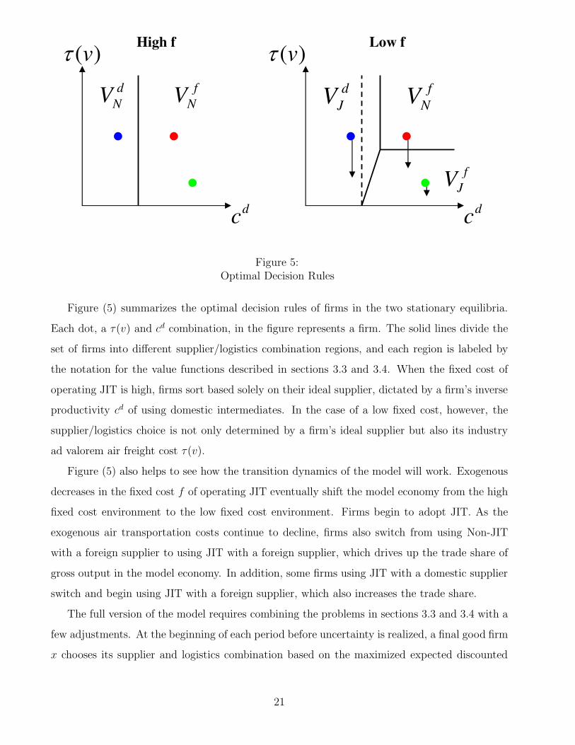
Figure (5) summarizes the optimal decision rules of firms in the two stationary equilibria.

Each dot, a τ(v) and cd combination, in the figure represents a firm. The solid lines divide the

set of firms into different supplier/logistics combination regions, and each region is labeled by

the notation for the value functions described in sections 3.3 and 3.4. When the fixed cost of

operating JIT is high, firms sort based solely on their ideal supplier, dictated by a firm’s inverse

productivity cd of using domestic intermediates. In the case of a low fixed cost, however, the

supplier/logistics choice is not only determined by a firm’s ideal supplier but also its industry

ad valorem air freight cost τ(v).

Figure (5) also helps to see how the transition dynamics of the model will work. Exogenous

decreases in the fixed cost f of operating JIT eventually shift the model economy from the high

fixed cost environment to the low fixed cost environment. Firms begin to adopt JIT. As the

exogenous air transportation costs continue to decline, firms also switch from using Non-JIT

with a foreign supplier to using JIT with a foreign supplier, which drives up the trade share of

gross output in the model economy. In addition, some firms using JIT with a domestic supplier

switch and begin using JIT with a foreign supplier, which also increases the trade share.

The full version of the model requires combining the problems in sections 3.3 and 3.4 with a

few adjustments. At the beginning of each period before uncertainty is realized, a final good firm

x chooses its supplier and logistics combination based on the maximized expected discounted

21

value of each choice:

V (s; x) = max{

V dN(s; x), V

fN(s; x), V

dJ (s; x), V

fJ (s; x)

}

, (20)

where

V dN(s; x) = max

pN ,z≥0

∫ z

ε

[

pNy(pN)ε− pmcd[y(pN)z − s]− pIy(pN)[z − ε] + βEτ(v),fV (s′; x)

]

dF (ε)

+

∫ ε

z

[

pNy(pN)z − pmcd[y(pN)z − s] + βEτ(v),fV (s′; x)

]

dF (ε), (21)

VfN(s; x) = max

pN ,z≥0

∫ z

ε

[

pNy(pN)ε− pm[y(pN)z − s]− pIy(pN)[z − ε] + βEτ(v),fV (s′; x)]

dF (ε)

+

∫ ε

z

[

pNy(pN)z − pm[y(pN)z − s] + βEτ(v),fV (s′; x)]

dF (ε), (22)

V dJ (s; x) = max

pJ ,q≥0pJy(pJ)E(ε)− pmc

dq − f + pss+ βEτ(v),fV (s′; x), (23)

and

VfJ (s; x) = max

pJ ,q≥0pJy(pJ)E(ε)− (1 + τ(v))pmq − f + pss+ βEτ(v),fV (s′; x). (24)

I write out all four value functions in hopes of clarifying the differences between each supplier

and logistics choice.27 In addition to the expectations over the distribution of demand shocks, a

firm also takes into account its expectations over the evolution of the fixed cost of operating JIT

and its air transportation cost. I write problem (20) in a flexible enough fashion to accommodate

a variety of expectations.28 The JIT problems (23) and (24) differ from their stationary coun-

terpart (13) by the inclusion of the term pss. The reason is straightforward. If a firm decides to

adopt JIT in the current period but operated Non-JIT in the previous period, then it is possible

the firm begins the period with a current stock of inventory s. ps represents a salvage value the

firm receives per unit of inventory. Notice ps can be positive or negative, though, depending on

its interpretation. ps > 0 represents the salvage value just described. ps < 0, however, poses an

additional cost on the firm for getting rid of its leftover inventory. An example might be the

27However, I continue to suppress the firm notation x on most variables.28I take a stand on the form of the expectations used in the numerical example presented in section 4.

22

need to tear down an old warehouse used to previously store inventory.

4 Numerical Example

In this section, I provide a numerical example to illustrate the mechanics of the model and show

the model is capable of capturing part of the growth in trade beginning in the early 1980’s.29

The experiment I run measures the trade share of gross output in the model economy for a given

set of parameter values and exogenous sequences of air transportation costs τ(v)’s and the fixed

cost f of operating the JIT technology. The model results are then compared with the trade

share in the data.

The model economy contains 6600 firms. Each firm belongs to a specific industry, and each

industry contains 100 firms. The 66 industries correspond to the same 66 SIC manufacturing

industries appearing in figure (4). The simulation is compared to the trade share data for U.S.

manufacturing over the period 1974-2004. For each year, I measure an industry’s ad valorem

air freight charge from the data in Hummels (2007) used to construct figure (4). These air

charges serve as the exogenous sequences of air transportation costs in the model. Figure (6)

shows two examples of the exogenous sequences of air transportation costs. Both structural clay

products and jewelry see a downward trend in their ad valorem air freight charge. Although

the downward trends suggest firms in both industries might eventually adopt JIT, the levels are

also important. From figure (4), it can be seen structural clay products have one of the highest

freight charges, whereas jewelry has one of the lowest. Firms in the jewelry industry will be

more likely to adopt JIT. The exogenous sequence of the fixed costs of operating JIT is chosen

so the fixed costs are high enough before the early 1980’s to limit the adoption of JIT and are

gradually reduced thereafter.

Table 1 summarizes the parameter values chosen for the numerical experiment. Firms receive

29The simulation presented here is a numerical example based on a simplified version of the full model developedin section 3. In particular, I 1) shut off the endogenous choice of the selling price pN of the final good and 2)assume no perfect foresight over the evolution of the air transportation costs and fixed cost of using JIT. Runningthe simulation with an exogenous pN versus an endogenous pN has little impact, since an exogenous pN can bechosen to be consistent with an endogenous pN given the choices of the other parameters. Assuming no perfectforesight appears on the surface more restrictive. Allowing firms some expectations over the evolution of the airtransportation costs and fixed cost might lead some firms to adopt JIT sooner. Given I choose the fixed cost tomatch the data fact that no firms use JIT before 1983, however, relaxing no perfect foresight would still resultin trade growth only after 1983. The growth in trade after 1983 might be faster without no perfect foresight.

23

0.00

0.20

0.40

0.60

0.80

1.00

1.20

0.00

0.01

0.02

0.03

0.04

1974 1979 1984 1989 1994 1999 2004

Sh

are

of

Va

lue

Sh

ipp

ed

, S

tru

ctu

ral

Cla

y P

rod

uc

ts

Sh

are

of

Va

lue

Sh

ipp

ed

, J

ew

elr

y Jewelry

Structural Clay Products

Figure 6:Ad Valorem Air Freight by Industry in U.S. Manufacturing, 1974-2004

their demand shocks each period from a uniform distribution with lower and upper bounds of 0.5

and 1.5. The scaling parameter of the demand function takes the value of 1, whereas the shape

parameter governing the elasticity is set to 6. At the beginning of the model simulation, each

firm draws its domestic inverse productivity cd from an exponential distribution with mean equal

to 5. The firm’s discount factor β is chosen to be 0.95. Firms using the Non-JIT technology sell

final goods at the exogenously set price pN = 7. Lastly, the price of inventorying a unit of the

final good is pI = 3, and the salvage value for selling off remaining inventories is ps = 0.

The results of the numerical example appear in figure (7). The model is capable of generating

a quantitatively large increase in the trade share of gross output, which in this example is nearly

half of the increase seen in the data. Given the exogenous sequences of the fixed cost and air

transportation costs, the model also replicates the increase in the trade share occurring in the

early 1980’s. By the early 1980’s, firms begin to adopt JIT with international suppliers, which

leads to the increase in the trade share around this period. As the fixed cost of adoption and

air transportation costs continue to decline, more and more firms adopt JIT with international

24

Table 1: Model Simulation ParametersParameter Description Value

a Demand Scale 1b Demand Shape 6ε Demand Shock Lower Bound 0.5ε Demand Shock Upper Bound 1.5µ Mean of Domestic Inverse Productivity Distribution 5β Firm Discount Factor 0.95pN Final Good Price, i = d, f 7pm Intermediate Good Price 5pI Unit Cost of Inventory 3ps Unit Salvage Value 0

0

50

100

150

200

250

300

350

400

1974 1979 1984 1989 1994 1999 2004

1974=

100

Data

Model

Figure 7:Model Simulation: Trade / Gross Output in U.S. Manufacturing

suppliers, further pushing up the trade share of gross output. Since the fixed cost and air

transportation costs continue to decline, the total number of new firms switching to JIT with

international suppliers begins to decrease. This results in the trade share eventually plateauing,

as the main mechanism in the model generating increased trade is the switching to JIT with

international suppliers. Since switching never occurs before the early 1980’s due to the high

fixed cost, the model’s trade share remains unchanged during this period. Changing the timing

25

-5

0

5

10

15

20

25

-8 -6 -4 -2 0 2 4 6

Average Annual Percentage Growth in I/S

Av

era

ge

An

nu

al

Pe

rce

nta

ge

Gro

wth

in

Im

po

rts

Computers

y = -0.6527x + 8.1848

(0.2745) (0.6771)

Figure 8:Trade and Inventory / Sales by Industry in U.S. Manufacturing, 1983-1996

of the decline in the fixed cost shifts the initial increase in the model’s trade share.

5 Further Empirical Evidence

This section presents evidence showing the predictions of the theory outlined in section 3 are

consistent with industry-level panel data for U.S. manufacturing. I do not intend to provide

a comprehensive empirical analysis of the industry data, because this is not the main focus of

my paper. Rather, my primary goal is to take an initial look across industries to test the main

implication of my theory, that the adoption of JIT is associated with increased trade volumes

and increased use of air transportation. A secondary goal I wish to achieve by showing the

regularities in the industry data is to highlight useful extensions of my theory and possible

avenues for future research.

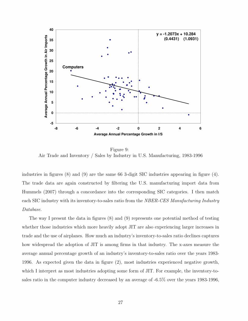
To this end, figures (8) and (9) document the relation between both the inventory-to-sales

ratio and the total value of imports and the inventory-to-sales ratio and the total value of

imports shipped by airplanes for U.S. manufacturing industries over the years 1983-1996. The

26

-5

0

5

10

15

20

25

30

35

40

-8 -6 -4 -2 0 2 4 6

Average Annual Percentage Growth in I/S

Av

era

ge

An

nu

al

Pe

rce

nta

ge

Gro

wth

in

Air

Im

po

rts

Computers

y = -1.2073x + 10.284

(0.4431) (1.0931)

Figure 9:Air Trade and Inventory / Sales by Industry in U.S. Manufacturing, 1983-1996

industries in figures (8) and (9) are the same 66 3-digit SIC industries appearing in figure (4).

The trade data are again constructed by filtering the U.S. manufacturing import data from

Hummels (2007) through a concordance into the corresponding SIC categories. I then match

each SIC industry with its inventory-to-sales ratio from the NBER-CES Manufacturing Industry

Database.

The way I present the data in figures (8) and (9) represents one potential method of testing

whether those industries which more heavily adopt JIT are also experiencing larger increases in

trade and the use of airplanes. How much an industry’s inventory-to-sales ratio declines captures

how widespread the adoption of JIT is among firms in that industry. The x-axes measure the

average annual percentage growth of an industry’s inventory-to-sales ratio over the years 1983-

1996. As expected given the data in figure (2), most industries experienced negative growth,

which I interpret as most industries adopting some form of JIT. For example, the inventory-to-

sales ratio in the computer industry decreased by an average of -6.5% over the years 1983-1996,

27

an industry often cited as a leader in the use of JIT techniques.30 The y-axis in figure (8)

measures the average annual percentage growth in the total value of an industry’s imports

over the years 1983-1996. Similarly, figure (9)’s y-axis measures the average annual percentage

growth in the total value of an industry’s imports shipped by air over the same period. In the

case of the computer industry, imports grew by an average 16.65%, whereas imports shipped by

air grew by an average of 20.24%.

Overall, the simple OLS regressions reported in figures (8) and (9) suggest the theory de-

veloped in this paper is consistent with industry-level data. In the case of total imports, the

coefficient on the inventory-to-sales variable is -0.6527 (0.2745), where the value in parentheses

is the standard error. The coefficient on the inventory-to-sales variable in the case of imports

shipped by air is -1.2073 (0.4431). The sign of the coefficient in each case matches that predicted

by the theory.

The model in section 3 easily extends to further explore differences across industries. Certain

industries might more readily adopt JIT, which could be modeled as heterogeneous fixed costs.

Heterogeneous fixed costs would help break the plateauing in the trade share seen in the example

in figure (7). Or, industries could be modeled as facing different demand volatilities. Higher

demand volatility makes the decision to adopt JIT more attractive. The theory outlined in this

paper should prove useful for studying these types of issues.

6 Conclusion

This paper argues the widespread adoption of JIT in the early 1980’s is a key to explaining

the growth in U.S. manufacturing trade. JIT links together three conspicuous changes in U.S.

manufacturing: the growth of the trade share of gross output, the decline in the inventory-

to-sales ratio, and the increased use of airplane transportation. I formalize an interpretation

of how JIT increases trade by developing a theory based on the logistics technology used in

30A recent colorful example appears in Friedman (2005). The author retells his experience of ordering a Dellnotebook computer and tracking the production process. Once the order is made, components from differentparts of the world are brought together and assembled to create a final product which is then delivered to theauthor. Streamlined communication and airplane transportation facilitate the different stages, from the orderingof the notebook to the delivery at its final destination, all of which normally takes place over the course of a fewdays.

28

a firm’s supply chain. Technological progress in the form of declining air transportation costs

and a declining fixed cost of JIT adoption leads firms to implement JIT, which increases trade

through the flexibility, price, and switching effects.

In addition to providing a deeper understanding of the forces driving the growth in aggregate

U.S. manufacturing trade, the theory I develop also serves as a useful framework for industry-

level studies, both those exploring differences across industries and those of a particular industry.

I have begun to explore the differences across industries by showing the theory is consistent

with industry-level panel data for U.S. manufacturing. Future research would prove useful in

deepening the understanding of the growth in U.S. manufacturing trade in particular and the

effects of JIT on trade in general.

Lastly, the theory provides new tools for evaluating the effects of government policies on

trade and the structure of manufacturing production. The model can accommodate traditional

policy experiments like the introduction of a tariff but also opens up new avenues for thinking

about policies which typically are not studied by international trade theorists. For example,

policies potentially affecting the cost of airplane transportation, such as Open Skies agreements,

can be evaluated for their impact on international trade flows and production.

29

Appendix

Appendix A: Stationary Non-JIT Problem

I adopt the sequential procedure used in Petruzzi and Dada (1999) to solve the Non-JIT firm’s

problem. The optimal value of pN is solved as a function of z. This price function is then

substituted back into the Non-JIT problem to solve for z. These solutions can then be used to

jointly determine the optimal values p∗N and z∗.

Recall equation (6), the Non-JIT firm’s problem when using either a domestic or an inter-

national supplier:

V iN(s; x) = max

pN≥0

∫ z

ε

[

pNy(pN)ε− pmci[y(pN)z − s]− pIy(pN)[z − ε] + βV i

N

(

y(pN)[z − ε]; x)]

dF (ε)

+

∫ ε

z

[

pNy(pN)z − pmci[y(pN)z − s] + βV i

N(0; x)]

dF (ε).

This problem can be rewritten as

V iN(s; x) = max

pN≥0

∫ z

ε

[

pNy(pN)ε− pmciy(pN)z − pIy(pN)[z − ε]

]

dF (ε)

+

∫ ε

z

[

pNy(pN)z + pNy(pN)ε− pNy(pN)ε− pmciy(pN)z

]

dF (ε)

+

∫ z

ε

βV iN

(

y(pN)[z − ε]; x)

dF (ε) +

∫ ε

z

βV iN(0; x)dF (ε) + pmc

is,

which after some algebra simplifies further to the following convenient form:

V iN(s; x) = max

pN≥0(pN − pmc

i)y(pN)E(ε)− y(pN)[

(pmci + pI)Λ(z) + (pN − pmc

i)Θ(z)]

+

∫ z

ε

βV iN

(

y(pN)[z − ε]; x)

dF (ε) +

∫ ε

z

βV iN(0; x)dF (ε) + pmc

is,

where Λ(z) =∫ z

ε(z− ε)dF (ε) and Θ(z) =

∫ ε

z(ε− z)dF (ε). Taking the FOC w.r.t. pN yields the

following:

y(pN)E(ε) + pNE(ε)∂y(pN)

∂pN− pmc

iE(ε)∂y(pN)

∂pN− (pmc

i + pI)Λ(z)∂y(pN )

∂pN− y(pN)Θ(z)

−pNΘ(z)∂y(pN )

∂pN+ pmc

iΘ(z)∂y(pN)

∂pN+ βpmc

iΛ(z)∂y(pN)

∂pN= 0.

30

Plugging in y(pN) = ap−bN and doing some algebra results in the following solution for the optimal

pN , equation (9):

p∗N =pmc

ib

b− 1+

(b

b− 1

)(

pmci − (βpmc

i − pI))

Λ(z)

[E(ε)−Θ(z)].

Since b > 1, 0 < β < 1, and E(ε)−Θ(z) > 0, it is clear p∗N > pmcib

b−1by simple inspection.

In order to solve for the form of the optimal z, note pN = pN(z). In what follows, I write pN ,

suppressing the z for notational simplicity. I first rewrite equation (6) by doing some algebra

and plugging in y(pN) = ap−bN :

V iN(s; x) = max

z≥0ap1−b

N E(ε)− pmciaE(ε)p−b

N − a(pmci + pI)Λ(z)p

−bN − aΘ(z)p1−b

N + apmciΘ(z)p−b

N

+β

∫ z

ε

V iN

(

ap−bN [z − ε]; x

)

dF (ε) + βV iN(0; x)− βV i

N(0; x)F (z) + pmcis.

Rewriting equation (6) in this way just provides me with a convenient form for taking the FOC

w.r.t. z:

(1− b)aE(ε)p−bN

∂pN

∂z+ bpmc

iaE(ε)p−b−1N

∂pN

∂z− a(pmc

i + pI)p−bN

∂Λ(z)

∂z+ ba(pmc

i + pI)Λ(z)p−b−1N

∂pN

∂z

−(1− b)aΘ(z)p−bN

∂pN

∂z− ap1−b

N

∂Θ(z)

∂z− bapmc

iΘ(z)p−b−1N

∂pN

∂z+ apmc

ip−bN

∂Θ(z)

∂z

+β∂∫ z

εV iN(ap

−bN [z − ε]; x)dF (ε)

∂z− βV i

N(0; x)∂F (z)

∂z= 0.

Solving for z is straightforward but requires tedious amounts of algebra. Some key steps are the

application of Leibniz’s rule for differentiation under an integral sign and to note ∂Λ(z)∂z

= F (z)

and ∂Θ(z)∂z

= F (z)− 1. Eventually, one derives

−pIF (z)− pNF (z) + pN − pmci + βpmc

iF (z) = 0,

which can be rewritten as the familiar critical fractile solution shown in equation (7):

z∗ = F−1

(pN − pmc

i

pN − (βpmci − pI)

)

.

Solving for the maximized expected discounted value of the Non-JIT technology involves

31

straightforward methods from dynamic programming. Here, I only show the step of guessing

and verifying the form of the value function. Recall equation (6):

V iN(s; x) = max

pN≥0

∫ z

ε

[

pNy(pN)ε− pmci[y(pN)z − s]− pIy(pN)[z − ε] + βV i

N

(

y(pN)[z − ε]; x)]

dF (ε)

+

∫ ε

z

[

pNy(pN)z − pmci[y(pN)z − s] + βV i

N(0; x)]

dF (ε).

Guess V iN(s; x) = B + pmc

is over [0, z∗], which implies V iN(0; x) = B. Plugging these into the

value function yields the following:

B =

∫ z

ε

[

pNy(pN)ε− pmciy(pN)z − pIy(pN)z + pIy(pN)ε+ β

[B + pmc

iy(pN)[z − ε]]]

dF (ε)

+

∫ ε

z

[

pNy(pN)z − pmciy(pN)z + βB

]

dF (ε).

B can then be solved after some tedious algebra:

B =(pN − pmc

i)y(pN)z

1− β−

y(pN)(pN − (βpmc

i − pI)) ∫ z

εF (ε)dε

1− β.

The maximized expected discounted value of the Non-JIT technology is then written as equation

(10):

V iN(s; x) =

y(p∗N)

1− β

[

(p∗N − pmci)z∗ −

(

p∗N − (βpmci − pI)

)∫ z∗

ε

F (ε)dε]

+ pmcis.

Appendix B: Trade-to-Gross Output Ratio in Non-JIT vs. JIT

In order to show equation (19), I show trade grows faster than gross output when switching

from Non-JIT with international suppliers to JIT with international suppliers:

TradeJIT − TradeNon−JIT

TradeNon−JIT

>GrossOutputJIT −GrossOutputNon−JIT

GrossOutputNon−JIT

.

Using equations (14) - (18), the LHS of the above can be rewritten as

pmy(p∗J)[ ∫ z∗

εεdF (ε) +

∫ ε

z∗εdF (ε)

]

− pmy(p∗N)

[ ∫ z∗

εεdF (ε) +

∫ ε

z∗z∗dF (ε)

]

pmy(p∗N)[ ∫ z∗

εεdF (ε) +

∫ ε

z∗z∗dF (ε)

]

32

and the RHS can be rewritten as

p∗Jy(p∗J)[ ∫ z∗

εεdF (ε) +

∫ ε

z∗εdF (ε)

]

− pIy(p∗N)

∫ z∗

ε(z∗ − ε)dF (ε)− p∗Ny(p

∗N)

[ ∫ z∗

εεdF (ε) +

∫ ε

z∗z∗dF (ε)

]

pIy(p∗N)

∫ z∗

ε(z∗ − ε)dF (ε) + p∗Ny(p

∗N)

[ ∫ z∗

εεdF (ε) +

∫ ε

z∗z∗dF (ε)

] .

After some algebra, the LHS and RHS can be simplified to the following:

y(p∗J)

y(p∗N)

[ ∫ z∗

εεdF (ε) +

∫ ε

z∗εdF (ε)

]

[ ∫ z∗

εεdF (ε) +

∫ ε

z∗z∗dF (ε)

]−1 > p∗Jy(p∗J)

y(p∗N)

[ ∫ z∗

εεdF (ε) +

∫ ε

z∗εdF (ε)

]

pI∫ z∗

ε(z∗ − ε)dF (ε) + p∗N

[ ∫ z∗

εεdF (ε) +

∫ ε

z∗z∗dF (ε)

]−1.

Again, after some algebra, this simplifies to

pI

∫ z∗

ε

(z∗ − ε)dF (ε) + (p∗N − p∗J)[ ∫ z∗

ε

εdF (ε) +

∫ ε

z∗z∗dF (ε)

]

> 0,

which holds true when p∗N > p∗J . p∗J can theoretically be higher than p∗N . This will rarely be the

case, however, since those firms choosing JIT are those with relatively lower air transportation

costs, which means their p∗J ’s are likely to be greater than their p∗N ’s. Recall, of course, that

switching from Non-JIT with international suppliers to JIT with international suppliers is not

the only mechanism through which the trade-to-gross output ratio increases. Switching from

JIT with domestic suppliers to JIT with international suppliers also increases the trade-to-gross

output ratio. This switching effect does not enter the above derivation.

33

References

Alessandria, G., and H. Choi (2008): “Do Falling Iceberg Costs Account for Recent US

Export Growth?,” Working Paper.

Arrow, K. J., T. Harris, and J. Marschak (1951): “Optimal Inventory Policy,” Econo-

metrica, 19(3), 250–272.

Bajona, C. (2004): “Specific Factors, Learning, and the Dynamics of Trade,” International

Economic Review, 45(2), 499–521.

Bergoeing, R., and T. J. Kehoe (2003): “Trade Theory and Trade Facts,” Federal Reserve

Bank of Minneapolis Staff Report 284.

Bergoeing, R., T. J. Kehoe, V. Strauss-Kahn, and K.-M. Yi (2004): “Why Is Man-

ufacturing Trade Rising Even as Manufacturing Output Is Falling?,” American Economic

Review Papers and Proceedings, 94(2), 134–138.

Bernanke, B. S. (2004): “The Great Moderation,” Speech at the meet-

ings of the Eastern Economic Association, Washington, D.C., February 20,

http://www.federalreserve.gov/BOARDDOCS/SPEECHES/2004/20040220/default.htm.

Blanchard, O., and J. Simon (2001): “The Long and Large Decline in U.S. Output Volatil-

ity,” Brookings Papers on Economic Activity, 2001(1), 135–164.

Bridgman, B. (2008): “Energy Prices and the Expansion of World Trade,” Review of Economic

Dynamics, 11(4), 904–916.

(2012): “The Rise of Vertical Specialization Trade,” Journal of International Eco-

nomics, 86(1), 133–140.

Cunat, A., and M. Maffezzoli (2007): “Can Comparative Advantage Explain the Growth

of U.S. Trade?,” Economic Journal, 117(520), 583–602.

Davis, S. J., and J. A. Kahn (2008): “Interpreting the Great Moderation: Changes in

the Volatility of Economic Activity at the Macro and Micro Levels,” Journal of Economic

Perspectives, 22(4), 155–180.

34

Edgeworth, F. (1888): “The Mathematical Theory of Banking,” Journal of the Royal Statis-

tical Society, 51(1), 113–127.

Estevadeordal, A., B. Frantz, and A. M. Taylor (2003): “The Rise and Fall of World

Trade, 1870-1939,” Quarterly Journal of Economics, 118(2), 359–407.

Feinberg, S. E., and M. P. Keane (2006): “Accounting for the Growth of MNC-Based Trade

Using a Structural Model of U.S. MNCs,” American Economic Review, 96(5), 1515–1558.

Friedman, T. L. (2005): The World Is Flat: A Brief History of the Twenty-First Century.

New York, NY: Farrar, Straus and Giroux.

Harrigan, J. (2010): “Airplanes and Comparative Advantage,” Journal of International Eco-

nomics, 82(2), 181–194.

Hayakawa, K. (2010): “The Choice of Transport Mode: Evidence from Japanese Exports to

East Asia,” Journal of the Korean Economy, 11(1), 195–209.

Hummels, D. (2001): “Time as a Trade Barrier,” Working Paper.

(2007): “Transportation Costs and International Trade in the Second Era of Global-

ization,” Journal of Economic Perspectives, 21(3), 131–154.

Hummels, D., and G. Schaur (2010): “Hedging Price Volatility Using Fast Transport,”

Journal of International Economics, 82(1), 15–25.

Kahn, J. A., M. M. McConnell, and G. Perez-Quiros (2002): “On the Causes of the

Increased Stability of the U.S. Economy,” Federal Reserve Bank of New York Economic Policy

Review, 8(1), 183–202.

Keane, M. P., and S. E. Feinberg (2007): “Advances in Logistics and the Growth of Intra-

Firm Trade: The Case of Canadian Affiliates of U.S. Multinationals, 1984-1995,” Journal of

Industrial Economics, 55(4), 571–632.

McConnell, M. M., and G. Perez-Quiros (2000): “Output Fluctuations in the United

States: What Has Changed Since the Early 1980’s?,” American Economic Review, 90(5),

1464–1476.

35

Ohno, T. (1988): Toyota Production System: Beyond Large-Scale Production. New York, NY:

Productivity Press.

O’Rourke, K. H., and J. G. Williamson (2002): “When Did Globalisation Begin?,” Eu-

ropean Review of Economic History, 6(1), 23–50.

Petruzzi, N. C., and M. Dada (1999): “Pricing and the Newsvendor Problem: A Review

With Extensions,” Operations Research, 47(2), 183–194.

Stock, J. H., and M. W. Watson (2003): “Has the Business Cycle Changed and Why?,”

NBER Macroeconomics Annual, 17(2002), 159–218.

Yi, K.-M. (2003): “Can Vertical Specialization Explain the Growth of World Trade?,” Journal

of Political Economy, 111(1), 52–102.

36