A Thread-Safe Arbitrary PrecisionComputation Package(Full Documentation)

David H. Bailey ∗

March 20, 2017

Abstract

Numerous research studies have arisen, particularly in the realmof mathematical physics and experimental mathematics, that requireextremely high numeric precision. Such precision greatly magnifiescomputer run times, so software packages to support high-precisioncomputing must be designed for thread-based parallel processing.

This paper describes a new package (“MPFUN2015”) that is thread-safe, even at the language interface level, yet still permits the workingprecision level to be freely changed during execution. The packagecomes in two versions: (a) a completely self-contained, all-Fortranversion that is simple to install; and (b) a version based on the MPFRpackage (for lower-level operations) that is more complicated to installbut is approximately 3X faster. Except for a few special functions, thetwo versions are “plug-compatible” in the sense that applications writ-ten for one also run with the other. Both versions employ advancedalgorithms, including FFT-based arithmetic, for optimal performance.They also detect, and provide means to overcome, accuracy problemsrooted in the usage of inexact double-precision constants and expres-sions. A high-level Fortran-90 interface, supporting both multipreci-sion real and complex datatypes, is provided for each, so that mostusers need only to make minor changes to existing code.

∗Lawrence Berkeley National Laboratory (retired), 1 Cyclotron Road, Berkeley, CA94720, USA, and University of California, Davis, Department of Computer Science. E-mail: david@davidhbailey.com.

1

Contents

1 Applications of high-precision computation 31.1 The PSLQ integer relation algorithm . . . . . . . . . . . . . . 31.2 High-precision numerical integration . . . . . . . . . . . . . . 41.3 Ising integrals . . . . . . . . . . . . . . . . . . . . . . . . . . . 51.4 Algebraic numbers in Poisson potential functions . . . . . . . 6

2 High-precision floating-point software 82.1 Available software packages . . . . . . . . . . . . . . . . . . . 82.2 Thread safety . . . . . . . . . . . . . . . . . . . . . . . . . . . 10

3 A thread-safe arbitrary precision computation package 123.1 Data structure . . . . . . . . . . . . . . . . . . . . . . . . . . . 143.2 Modules . . . . . . . . . . . . . . . . . . . . . . . . . . . . . . 153.3 The MPFUN2015 solution to thread safety . . . . . . . . . . . 15

4 Numerical algorithms used in MPFUN-Fort 174.1 Algorithms for basic arithmetic . . . . . . . . . . . . . . . . . 174.2 FFT-based multiplication . . . . . . . . . . . . . . . . . . . . 184.3 Advanced algorithm for division . . . . . . . . . . . . . . . . . 194.4 Basic algorithms for transcendental functions . . . . . . . . . . 204.5 Advanced algorithms for transcendental functions . . . . . . . 214.6 Special functions . . . . . . . . . . . . . . . . . . . . . . . . . 23

5 Installation, compilation and linking 26

6 Fortran coding instructions 276.1 Functions and subroutines . . . . . . . . . . . . . . . . . . . . 306.2 Input and output of multiprecision data . . . . . . . . . . . . 306.3 Handling double precision values . . . . . . . . . . . . . . . . 346.4 Dynamically changing the working precision . . . . . . . . . . 36

7 Performance of sample applications 387.1 Timings . . . . . . . . . . . . . . . . . . . . . . . . . . . . . . 40

8 Conclusion 40

2

1 Applications of high-precision computation

For many scientific calculations, particularly those that employ empiricaldata, IEEE 32-bit floating-point arithmetic is sufficiently accurate, and ispreferred since it saves memory, run time and energy usage. For other ap-plications, 64-bit floating-point arithmetic is required to produce results ofsufficient accuracy, although some users find that they can obtain satisfac-tory results by switching between 32-bit and 64-bit, using the latter only forcertain numerically sensitive sections of code. Software tools are being de-veloped at the University of California, Berkeley and elsewhere to help usersdetermine which portions of a computation can be performed with lowerprecision and which must be performed with higher precision [26].

Other applications, particularly in the fields of mathematical physics andexperimental mathematics, require even higher precision — tens, hundredsor even thousands of digits. Here is a brief summary of these applications:

1. Supernova simulations (32–64 digits).

2. Optimization problems in biology and other fields (32–64 digits).

3. Coulomb n-body atomic system simulations (32–120 digits).

4. Electromagnetic scattering theory (32–100 digits).

5. The Taylor algorithm for ODEs (100–600 digits).

6. Ising integrals from mathematical physics (100–1000 digits).

7. Problems in experimental mathematics (100–50,000 digits and higher).

These applications are described in greater detail in [1, 3], which providesdetailed references. Here is a brief overview of a handful of these applications:

1.1 The PSLQ integer relation algorithm

Very high-precision floating-point arithmetic is now considered an indispens-able tool in experimental mathematics and mathematical physics [1]. Manyof these computations involve variants of Ferguson’s PSLQ integer relationdetection algorithm [17, 8]. Suppose one is given an n-long vector (xi) of real

3

or complex numbers (presented as a vector of high-precision values). ThePSLQ algorithm finds the integer coefficients (ai), not all zero, such that

a1x1 + a2x2 + · · ·+ anxn = 0

(to available precision), or else determines that there is no such relationwithin a certain bound on the size of the coefficients. Alternatively, one canemploy the Lenstra-Lenstra-Lovasz (LLL) lattice basis reduction algorithmto find integer relations [22], or the “HJLS” algorithm, which is based on LLL.Both PSLQ and HJLS can be viewed as schemes to compute the intersectionbetween a lattice and a vector subspace [14]. Whichever algorithm is used,integer relation detection requires very high precision—at least (n× d)-digitprecision, where d is the size in digits of the largest ai and n is the vectorlength, or else the true relation will be unrecoverable.

1.2 High-precision numerical integration

One of the most fruitful applications of the experimental methodology andthe PSLQ integer relation algorithm has been to identify classes of definiteintegrals, based on very high-precision numerical values, in terms of simpleanalytic expressions.

These studies typically employ either Gaussian quadrature or the “tanh-sinh” quadrature scheme of Takahasi and Mori [27, 2]. The tanh-sinh quadra-ture algorithm approximates the integral of a function on (−1, 1) as∫ 1

−1f(x) dx ≈ h

N∑j=−N

wjf(xj), (1)

where the abscissas xj and weights wj are given by

xj = tanh (π/2 · sinh(hj))

wj = π/2 · cosh(hj)/ cosh (π/2 · sinh(hj))2 , (2)

and where N is chosen large enough that summation terms in (1) beyond N(positive or negative) are smaller than the “epsilon” of the numeric precisionbeing used. Full details are given in [2]. An overview of applications ofhigh-precision integration in experimental mathematics is given in [4].

4

1.3 Ising integrals

In one study, tanh-sinh quadrature and PSLQ were employed to study thefollowing classes of integrals [7]. The Cn are connected to quantum fieldtheory, the Dn integrals arise in the Ising theory of mathematical physics,while the En integrands are derived from Dn:

Cn =4

n!

∫ ∞0

· · ·∫ ∞0

1(∑nj=1(uj + 1/uj)

)2 du1u1· · · dun

un

Dn =4

n!

∫ ∞0

· · ·∫ ∞0

∏i<j

(ui−ujui+uj

)2(∑n

j=1(uj + 1/uj))2 du1

u1· · · dun

un

En = 2

∫ 1

0

· · ·∫ 1

0

( ∏1≤j<k≤n

uk − ujuk + uj

)2

dt2 dt3 · · · dtn.

In the last line uk =∏k

i=1 ti.In general, it is very difficult to compute high-precision numerical values of

n-dimensional integrals such as these. But as it turn out, the Cn integrals canbe converted to one-dimensional integrals, which are amenable to evaluationwith the tanh-sinh scheme:

Cn =2n

n!

∫ ∞0

pKn0 (p) dp.

Here K0 is the modified Bessel function [24]. 1000-digit values of these suf-ficed to identify the first few instances of Cn in terms of well-known constants.For example, C4 = 7ζ(3)/12, where ζ denotes the Riemann zeta function.For larger n, it quickly became clear that the Cn approach the limit

limn→∞

Cn = 0.630473503374386796122040192710 . . . .

This numerical value was quickly identified, using the Inverse Symbolic Cal-culator 2.0 (now available at http://carma-lx1.newcastle.edu.au:8087), as

limn→∞

Cn = 2e−2γ,

where γ is Euler’s constant. This identity was then proven [7].

5

Other specific results found in this study include the following:

D3 = 8 + 4π2/3− 27 L−3(2)

D4 = 4π2/9− 1/6− 7ζ(3)/2

E2 = 6− 8 log 2

E3 = 10− 2π2 − 8 log 2 + 32 log2 2

E4 = 22− 82ζ(3)− 24 log 2 + 176 log2 2− 256(log3 2)/3

+16π2 log 2− 22π2/3

E5 = 42− 1984 Li4(1/2) + 189π4/10− 74ζ(3)− 1272ζ(3) log 2 + 40π2 log2 2

−62π2/3 + 40(π2 log 2)/3 + 88 log4 2 + 464 log2 2− 40 log 2,

where ζ is the Riemann zeta function and Lin(x) is the polylog function.E5 was computed by first reducing it to a 3-D integral of a 60-line in-

tegrand, which was evaluated using tanh-sinh quadrature to 250-digit arith-metic using over 1000 CPU-hours on a highly parallel system. The PSLQcalculation required only seconds to produce the relation above. This formularemained a “numerical conjecture” for several years, but was proven in March2014 by Erik Panzer, who mentioned that he relied on these computationalresults to guide his research.

1.4 Algebraic numbers in Poisson potential functions

The Poisson equation arises in contexts such as engineering applications,the analysis of crystal structures, and even the sharpening of photographicimages. In two recent studies [5, 6], the present author and others exploredthe following class of sums:

φn(r1, . . . , rn) =1

π2

∑m1,...,mn odd

eiπ(m1r1+···+mnrn)

m21 + · · ·+m2

n

. (3)

After extensive high-precision numerical experimentation using (??), we dis-covered (then proved) the remarkable fact that when x and y are rational,

φ2(x, y) =1

πlogA, (4)

where A is an algebraic number, namely the root of an algebraic equationwith integer coefficients.

6

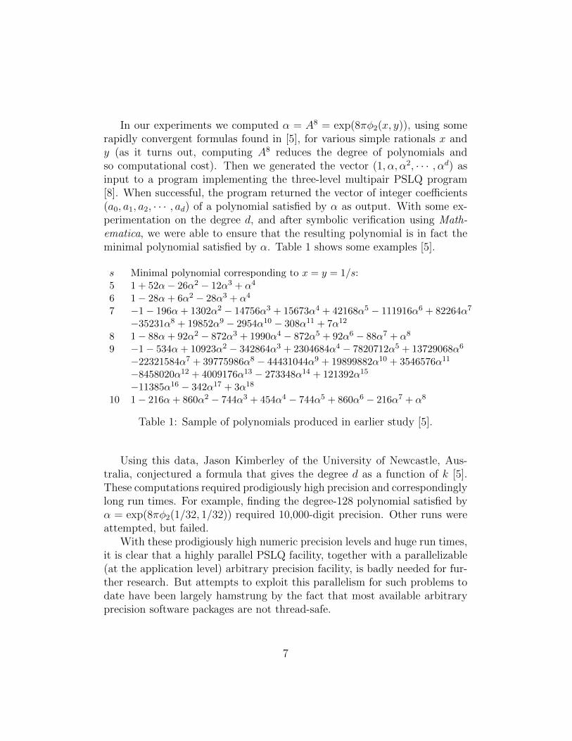
In our experiments we computed α = A8 = exp(8πφ2(x, y)), using somerapidly convergent formulas found in [5], for various simple rationals x andy (as it turns out, computing A8 reduces the degree of polynomials andso computational cost). Then we generated the vector (1, α, α2, · · · , αd) asinput to a program implementing the three-level multipair PSLQ program[8]. When successful, the program returned the vector of integer coefficients(a0, a1, a2, · · · , ad) of a polynomial satisfied by α as output. With some ex-perimentation on the degree d, and after symbolic verification using Math-ematica, we were able to ensure that the resulting polynomial is in fact theminimal polynomial satisfied by α. Table 1 shows some examples [5].

s Minimal polynomial corresponding to x = y = 1/s:5 1 + 52α− 26α2 − 12α3 + α4

6 1− 28α+ 6α2 − 28α3 + α4

7 −1− 196α+ 1302α2 − 14756α3 + 15673α4 + 42168α5 − 111916α6 + 82264α7

−35231α8 + 19852α9 − 2954α10 − 308α11 + 7α12

8 1− 88α+ 92α2 − 872α3 + 1990α4 − 872α5 + 92α6 − 88α7 + α8

9 −1− 534α+ 10923α2 − 342864α3 + 2304684α4 − 7820712α5 + 13729068α6

−22321584α7 + 39775986α8 − 44431044α9 + 19899882α10 + 3546576α11

−8458020α12 + 4009176α13 − 273348α14 + 121392α15

−11385α16 − 342α17 + 3α18

10 1− 216α+ 860α2 − 744α3 + 454α4 − 744α5 + 860α6 − 216α7 + α8

Table 1: Sample of polynomials produced in earlier study [5].

Using this data, Jason Kimberley of the University of Newcastle, Aus-tralia, conjectured a formula that gives the degree d as a function of k [5].These computations required prodigiously high precision and correspondinglylong run times. For example, finding the degree-128 polynomial satisfied byα = exp(8πφ2(1/32, 1/32)) required 10,000-digit precision. Other runs wereattempted, but failed.

With these prodigiously high numeric precision levels and huge run times,it is clear that a highly parallel PSLQ facility, together with a parallelizable(at the application level) arbitrary precision facility, is badly needed for fur-ther research. But attempts to exploit this parallelism for such problems todate have been largely hamstrung by the fact that most available arbitraryprecision software packages are not thread-safe.

7

2 High-precision floating-point software

By far the most common form of extra-precision arithmetic is roughly twicethe level of standard 64-bit IEEE floating-point arithmetic. One option is theIEEE standard for 128-bit binary floating-point arithmetic, with 113 man-tissa bits, but sadly it is not yet widely implemented in hardware, althoughit is supported, in software, in some compilers.

Another software option for this level of precision is “double-double”arithmetic (approximately 31-digit accuracy). This datatype consists of apair of 64-bit IEEE floats (s, t), where s is the 64-bit floating-point valueclosest to the desired value, and t is the difference (positive or negative)between the true value and s. One can extend this design to quad-doublearithmetic, which operates on strings of four IEEE 64-bit floats, providingroughly 62-digit accuracy. These two datatypes are supported by the QDpackage, which includes high-level language interfaces for C++ and Fortran(see below) [21].

For higher-levels of precision, software packages typically represent a high-precision datum as a string of floats or integers, where the first few wordscontain bookkeeping information and the binary exponent, and subsequentwords (except perhaps near the end) contain the mantissa. For moderate pre-cision levels (up to roughly 1000 digits), arithmetic on such data is typicallyperformed using adaptations of familiar schemes.

Above about 1000 or 2000 decimal digits, advanced algorithms should beemployed for maximum efficiency. For example, a high-precision multiply op-eration can be performed by noting that the key operation is merely a linearconvolution, which may be performed using fast Fourier transforms (FFTs).Efficient implementations of this scheme can dramatically accelerate multi-plication, since the FFT reduces an O(n2) operation to an O(n log n log log n)operation [13, Section 2.3] (see also Section 4.2).

2.1 Available software packages

Software for performing high-precision arithmetic has been available for quitesome time, for example in the commercial packages Mathematica and Maple.However, until 10 or 15 years ago, those with applications written in moreconventional languages, such as C++ or Fortran-90, often found it necessaryto rewrite their codes, replacing each arithmetic operation with a subroutinecall, which was a very tedious and error-prone process. Nowadays there

8

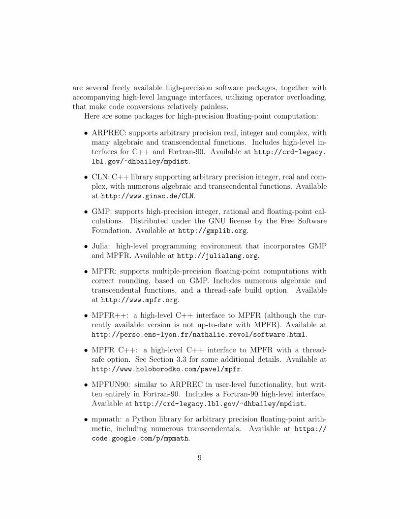
are several freely available high-precision software packages, together withaccompanying high-level language interfaces, utilizing operator overloading,that make code conversions relatively painless.

Here are some packages for high-precision floating-point computation:

• ARPREC: supports arbitrary precision real, integer and complex, withmany algebraic and transcendental functions. Includes high-level in-terfaces for C++ and Fortran-90. Available at http://crd-legacy.

lbl.gov/~dhbailey/mpdist.

• CLN: C++ library supporting arbitrary precision integer, real and com-plex, with numerous algebraic and transcendental functions. Availableat http://www.ginac.de/CLN.

• GMP: supports high-precision integer, rational and floating-point cal-culations. Distributed under the GNU license by the Free SoftwareFoundation. Available at http://gmplib.org.

• Julia: high-level programming environment that incorporates GMPand MPFR. Available at http://julialang.org.

• MPFR: supports multiple-precision floating-point computations withcorrect rounding, based on GMP. Includes numerous algebraic andtranscendental functions, and a thread-safe build option. Availableat http://www.mpfr.org.

• MPFR++: a high-level C++ interface to MPFR (although the cur-rently available version is not up-to-date with MPFR). Available athttp://perso.ens-lyon.fr/nathalie.revol/software.html.

• MPFR C++: a high-level C++ interface to MPFR with a thread-safe option. See Section 3.3 for some additional details. Available athttp://www.holoborodko.com/pavel/mpfr.

• MPFUN90: similar to ARPREC in user-level functionality, but writ-ten entirely in Fortran-90. Includes a Fortran-90 high-level interface.Available at http://crd-legacy.lbl.gov/~dhbailey/mpdist.

• mpmath: a Python library for arbitrary precision floating-point arith-metic, including numerous transcendentals. Available at https://

code.google.com/p/mpmath.

9

• NTL: a C++ library for arbitrary precision integer and floating-pointarithmetic. Available at http://www.shoup.net/ntl.

• Pari/GP: a computer algebra system that includes facilities for high-precision arithmetic, with many transcendental functions. Available athttp://pari.math.u-bordeaux.fr.

• QD: includes routines to perform “double-double” (approx. 31 digits)and “quad-double” (approx. 62 digits) arithmetic, as well as manyalgebraic and transcendental functions. Includes high-level interfacesfor C++ and Fortran-90. Available at http://crd-legacy.lbl.gov/

~dhbailey/mpdist.

• Sage: an open-source symbolic computing system that includes high-precision facilities. Available at http://www.sagemath.org.

2.2 Thread safety

The scientific computing world is moving rapidly into multicore and multi-node parallel computing, because the frequency and performance of individ-ual processors is no longer rapidly increasing [28]. Thus it is clear that futureimprovements in performance on high-precision computations will only beobtained by aggressively exploiting parallelism. It is difficult to achieve sig-nificant parallel speedup within a single high-precision arithmetic operation,but parallelization at the application level, e.g., parallelizing a DO or FORloop in an application code, is an attractive option.

It is possible to perform some high-precision computations in parallel byutilizing message passing interface (MPI) software at the application level.MPI employs a “shared none” environment that avoids many difficulties.Indeed, several high-precision applications have been performed on highlyparallel systems using MPI, including the study mentioned in Section 1.3 [7].

But on modern systems that feature multicore processors, parallel com-puting is more efficiently performed using a shared memory, multithreadedenvironment such as OpenMP [28] within a single node, even if MPI isemployed for parallelism between nodes. Furthermore, algorithms such asPSLQ, for example, can only be parallelized efficiently at a rather low looplevel — MPI implementations are not effective here unless the precision levelis exceedingly high.

10

Computations that use a thread-parallel environment such as OpenMPmust be entirely “thread-safe,” which means, among other things, that thereis no read/write global data, because otherwise there may be difficultieswith processors stepping on each other during parallel execution. Employing“locks” and the like may remedy such difficulties, but this reduces parallelefficiency and is problematic for code portability and installation.

One impediment to thread safety is the design of the operator overloadingfeature of modern computer languages, which is the only reasonable way toprogram a complicated high-precision calculation. Here “operator overload-ing” means the feature, available in several high-level languages includingC++ and Fortran-90, where algebraic operators, e.g., +, -, * and /, are ex-tended to high-precision operands. Such facilities typically do not permitone to carry information such as the current working precision level.

Most arbitrary precision packages generate a “context” of auxiliary data,such as the current working precision level and data to support transcenden-tal function evaluation. Such data, if not handled properly, can ruin threadsafety. For most high-precision computation packages, the available docu-mentation makes no statement one way or the other (which almost certainlymeans that they are not thread-safe).

Of the packages listed in Section 2, only one is a certified thread-safe,high-level floating-point package (i.e., uses operator overloading to interfacewith ordinary source code), namely the MPFR C++ package [23], whichis built upon the lower-level MPFR package [19]. The MPFR package inturn is very well-designed, features correct rounding to the last bit, includesnumerous transcendental and special functions, and achieves the the fastestoverall timings of any floating-point package in the above list [15].

According to the documentation, the MPFR package has a “thread-safebuild option.” When this is invoked, the package generates a context, local tothe thread, to support computation of certain transcendental functions at aparticular precision level, whenever a high-precision operation is initiated inthat thread. This is not ideal, since it means that if one is using thread-basedparallelism to parallelize a low-level loop, this context must be generated atthe start of each thread and freed at the end of the thread. However, one ofthe developers of MPFR has promised to the present author that in a futureversion, this context can be generated in a one-time initialization, after whichall computation will be thread-safe.

There is, to this author’s knowledge, no high-level, thread-safe arbitraryprecision package to support Fortran applications, prior to the present work.

11

While thread safety is of paramount importance, several other lessonsshould be noted when designing a high-precision floating-point arithmeticfacility, based on the present author’s experience:

• Double precision constants and expressions pose a serious problem,since they are not automatically converted to high precision due tooperator precedence rules in most programming languages. A highpercentage of accuracy failures reported to the present author by usersof his earlier packages (ARPREC, MPFUN90 and QD) are due to theusage of inexact double precision values.

• Complicated installation scripts are problematic. Many support in-quiries for the author’s earlier packages have been for installation is-sues, not the underlying multiprecision software. Some users preferolder, out-of-date software, simply because it is easy to install.

• Special system settings, system-dependent features and exotic languagefeatures pose serious difficulties for portability and maintenance.

• As with any software activity, long-term support is a nagging issue.

3 A thread-safe arbitrary precision computa-

tion package

With this background, the present author has developed a new softwarepackage for arbitrary-precision computation, named “MPFUN2015.” It isavailable in two versions: (a) MPFUN-Fort, a completely self-contained, all-Fortran version that is simple to install; and (b) MPFUN-MPFR, a versionbased on the MPFR package for lower-level operations that is more compli-cated to install but is approximately 3X faster for most applications. Exceptfor a few special functions, the two versions are “plug-compatible” in thesense that applications written for one will also run with the other withoutany changes (see Section 6.4 for details). These versions feature:

1. Full support for both real and complex datatypes, including all basicarithmetic operations and transcendental functions. A full-featuredhigh-level language interface for Fortran-90 is provided, so that mostusers need only make minor changes to existing double precision code.A C++ interface is planned but is not yet written.

12

2. A 100% thread safe design, even at the user language interface level,since no “context” or auxiliary data needs to be generated (unless ex-ceedingly high precision is used). The working precision can be freelychanged (up to a flexible limit) during execution, even in low-levelloops, without ruining thread safety. See however Section 3.3.

3. Numerous transcendental functions and special functions, includingmost of the intrinsic funtions specified in the Fortran-2008 standard.See Section 6.1 for a complete listing.

4. There is no need to manually allocate or deallocate temporary multi-precision variables or arrays in subroutines — all such data works withthe standard automatic array feature of Fortran, and is thread-safe.

5. No system-dependent features or settings. Proper operation does notdepend on the IEEE rounding mode of the user application (althoughsee item 11 below).

6. Straightforward installation, using scripts provided for various envi-ronments. MPFUN-Fort is supported with the GNU, IBM, Intel andPortland Group Fortran compilers, and MPFUN-MPFR is supportedon the GNU and Intel Fortran compilers, provided that the gcc com-piler is also available for installation of GMP and MPFR.

7. Precision is theoretically scalable to millions of decimal digits, althoughat present the MPFUN-Fort version is limited to 1.2 million digits.

8. Advanced algorithms, including FFT-based arithmetic, are employedin both versions for top performance even at very high precision levels.

9. A highly effective solution is provided to the double precision accuracyproblem mentioned in Section 2.2.

10. The overall runtime performance of the MPFUN-Fort version is some-what faster than the present author’s ARPREC package; the MPFUN-MPFR version is roughly 3X faster than either on large problems.

11. With the MPFUN-MPFR version, computations are guaranteed accu-rate to the last bit. However both versions perform computations toone more word (14–19 digits) of precision than requested by the user,minimizing roundoff error.

13

3.1 Data structure

For the MPFUN-Fort version, the structure is a (N +6)-long vector of 64-bitIEEE floating-point words, where N is the number of manttisa words:

• Word 0: Total space allocated for this array, in 64-bit words.

• Word 1: The working precision level (in words) associated with thisdata.

• Word 2: The number of mantissa words N ; the sign of word 2 is thesign of the value.

• Word 3: The multiprecision exponent, base 248.

• Word 4 to N + 3: N mantissa words (whole numbers between 0 and248 − 1).

• Word N + 4 and N + 5: Scratch words for internal usage.

For the MPFUN-MPFR version, the structure is a (N + 6)-long vector of64-bit integers:

• Word 0: Total space allocated for this array, in 64-bit words.

• Word 1: The working precision level (in bits) associated with this data.

• Word 2: The sign of the value.

• Word 3: The exponent, base 2.

• Word 4: A pointer to the first word of the mantissa, which in MPFUN-MPFR always points to Word 5.

• Word 5 to N + 4: Mantissa words (unsigned integers between 0 and264 − 1).

• N + 5: Not used at present.

Note that in the MPFUN-MPFR version, words 1 through N + 4 correspondexactly to the data structure of the MPFR package.

For both versions, a complex multiprecision datatype is a contiguous pairof real multiprecision data. Note that the imaginary member of the real-imaginary pair starts at an offset in the array equal to the value of word 0.Note also that this offset is independent of the working precision.

14

3.2 Modules

The MPFUN-Fort software includes the following separate modules, each inits own source file:

1. MPFUNA: Contains compile-time global data. In the MPFUN-Fortversion, this module includes data to support FFT-based arithmeticand binary values of log 2, π and 1/

√2 (up to 19,500-digit precision).

2. MPFUNB (present only in MPFUN-Fort): Handles basic arithmeticfunctions, rounding, normalization, square roots and n-th roots. TheFFT-based arithmetic facility to support very high precision computa-tion is included in this module.

3. MPFUNC (present only in MPFUN-Fort): Handles binary-to-decimalconversion, decimal-to-binary conversion and input/output operations.

4. MPFUND (present only in MPFUN-Fort): Includes routines for allcommon transcendental constants and functions, as well as special rou-tines, implementing advanced algorithms, for very high precision levels.

5. MPFUNE (present only in MPFUN-Fort): Includes routines for specialfunctions, such as the BesselJ, gamma, incomplete gamma and zetafunctions.

6. MPFUNF: Defines the default (maximum) precision. This is the onlymodule that needs to be modified by the user.

7. MPFUNG: A high-level user interface that connects to user code viaoperator overloading and function extension.

8. MPMODULE: The main module that references the others and is ref-erenced by the user.

3.3 The MPFUN2015 solution to thread safety

All of the software modules above are 100% thread safe. There are no globalparameters or arrays, except for static, compile-time data, and no initial-ization is required unless extremely high precision is required. For both theMPFUN-Fort and MPFUN-MPFR versions, working precision level is passedas a subroutine argument, ensuring thread safety. For the MPFUN-MPFR

15

version, for the time being thread safety cannot be guaranteed unless theuser’s code does not involve transcendental functions in multi-threaded sec-tions of code. This limitation will be removed in a future release.

Thread safety at the language interface or user level in both versions isachieved by assigning a working precision level to each multiprecision datum,which then is passed through the multiprecision software. Note, in the datastructure for both MPFUN-Fort and MPFUN-MPFR given in Section 3.1above, that word 1 (the second word of the array) is the working precisionlevel associated with that datum. This solves the thread safety problem whenprecision is dynamically changed in the application, although it requires asomewhat different programming style, as we shall briefly explain here (seeSection 6.4 for additional details).

To use either version from a Fortran program, the user first sets the pa-rameter mpipl, the “default” precision level in digits, which is the maximumprecision level to be used for subsequent computation, and is used to set theamount of storage required for multiprecision data. mpipl is set in a param-eter statement at the start of module MPFUNF, which is in file mpfunf.f90.In the code as distributed, mpipl is set to 1200 digits (sufficient to run thesix test problems of Section 7), but it can be set to any level greater than orequal to 30 digits. mpipl is converted to mantissa words (parameter mpwds),which is the internal default precision level.

All computations are performed to mpwds words precision unless the user,in an application code, specifies a lower value. During execution, the user canchange the working precision assigned to a multiprecision variable or array byusing the built-in functions mpreal and mpcmplx (see Section 6.4 for details).The working precision level assigned to a particular multiprecision variableor array element can be monitored using the built-in function mpwprec.

During execution, the result of any operation involving multiprecisionvariables or array elements “inherits” the working precision level of the inputoperands (if the operands have different working precision levels, the higherprecision level is chosen for the result). When assigning a multiprecisionvariable or array element to double precision constant or variable, or whenreading multiprecision data from a file, the result is assigned the defaultprecision unless a lower precision level is specified.

16

4 Numerical algorithms used in MPFUN-Fort

As mentioned above, MPFUN-MPFR relies on MPFR for all lower-levelarithmetic operations and transcendental functions, whereas MPFUN-Fort iscompletely self-contained. The algorithms employed in the MPFR packageare described in [19]. This section presents a brief overview of the algorithmsused in MPFUN-Fort. Those readers primarily interested in MPFUN-MPFRmay skip to Section 5.

4.1 Algorithms for basic arithmetic

Multiplication. For modest levels of precision, MPFUN-Fort employs adap-tations of the usual schemes we all learned in grade school, where the numberbase is 248 = 281474976710656 instead of ten. In the inner loop of the mul-tiplication routine division routines, note that two such numbers a and b inthe range [0, 248) must be multiplied, obtaining the exact 96-bit result.

This is performed in MPFUN-Fort by splitting both a and b into high- andlow-order 24-bit parts, using the sequence of operations a1 = 224 int (2−24a),a2 = a−a1. Note that a = a1+a2. If the four half-sized values are a1, a2, b1, b2,then calculate c = a1 ·b2+a2 ·b1, then c1 = 248 int 2−48(c), c2 = c−c1. Finallycalculate d1 = 2−48(a1 ·b1+c1), d2 = a2 ·b2+c2. Then d1 and d2 are the high-and low-order 48-bit mantissa words of the product, with the proviso thatalthough d = d1 + d2 = a · b is mathematically correct, d1 and d2 might notbe the precisely correct split into two words in the range [0, 248). However,since a double precision datatype can exactly hold whole numbers up to 253

in size, no accuracy is lost. In fact, this operation can be repeatedly done ina loop, provided that this data is periodically corrected in a normalizationoperation. Note also that the splitting of data in at least one of the twoarguments at the beginning can be done outside the inner loop.

The resulting scheme is very efficient yet totally reliable — in effect, itperforms quad precision with only a handful of register-level operations. Notealso that if two n-word arguments are multiplied, and the working precisionis also n words, then since only an n-word result is returned, only slightlymore than half of the “multiplication pyramid” need be calculated.

Division. A similar approach can be taken to division. Again, the key step isto inexpensively simulate quad precision in the inner loop, using the schemeoutlined above.

17

Square roots. Square roots are calculated by the following Newton-Raphsoniteration, which converges to 1/

√a [10, pg. 227]:

xk+1 = xk + 1/2 · (1− x2k · a) · xk, (5)

where the multiplication () · xk is performed with only half of the normallevel of precision. These iterations are performed with a working precisionlevel that approximately doubles with each iteration, except that at threeiterations before the final iteration, the iteration is repeated without doublingthe precision, in order to enhance accuracy. The final iteration is performedas follows (due to A. Karp):

√a ≈ (a · xn) + 1/2 · [a− (a · xn)2] · xn, (6)

where the multiplications (a ·xn) and [] ·xn are performed with only half thefinal level of precision. If this is done properly, the total cost of the calculationis only about three times the cost of a single full-precision multiplication.

n-th roots. A similar scheme is used to compute n-th roots for any integern. Computing xnk , which is required here, can be efficiently performed usingthe binary algorithm for exponentiation. This is merely the observation thatexponentiations can be accelerated based on the binary expansion of theexponent: for example, 317 can be computed as ((((3)2)2)2)2 ·3 = 129140163.

Note that these algorithms are trivially thread-safe, since no auxiliarydata is involved.

4.2 FFT-based multiplication

Although the multiplication algorithm described above is very efficient, forhigher levels of precision (above approximately 2500 digits, based on thepresent author’s implementation), significantly faster performance can beachieved by employing an FFT-convolution approach [13][10, pg. 223–224].

Suppose one wishes to multiply two n-precision values whose mantissawords are given by a = (a0, a1, a2, · · · , an−1) and b = (b0, b1, b2, · · · , bn−1). Itis easy to see that the desired result, except for releasing carries, is an acyclicconvolution. In particular, assume that a and b are extended to 2n wordseach by padding with zeroes. Then the product c = (ck) is given by

ck =2n−1∑j=0

ajbk−j, 0 ≤ k < 2n, (7)

18

where bk−j is read as bk−j+2n when k− j is negative. This convolution can becalculated as (c) = F−1[F (a) · F (b)], where F (a) and F (b) denote a real-to-complex discrete Fourier transform (computed using an FFT algorithm), thedot means element-by-element complex multiplication, and F−1[] means aninverse complex-to-real FFT. The ck results from this process are floating-point numbers. Rounding these values to the nearest integer, and then re-leasing carries beginning at c2n−1 gives the desired multiplication result.

The FFT-based multiplication facility of the present MPFUN-Fort soft-ware supports a precision level up to approximately 1.2 million digits. Be-yond this level, numerical round-off error in the FFT is too great to reliablyround the ck results to the nearest integer. If the maximum rounding errorexceeds 0.375 (beyond which is deemed unsafe), an error message is out-put. A planned future enhancement to MPFUN-Fort will extend the usableprecision level to at least 100 million decimal digits.

In contrast to the basic arithmetic algorithms, FFT-based multiplicationrequires precomputed FFT root-of-unity data. However, all the requisiteFFT data to support any precision level up to 19,500 digits is stored asstatic data in module MPFUNA. Thus up to this level, MPFUN-Fort requiresno initialization, and is completely thread-safe (since no “context” must becreated or freed). If even higher precision is required, the requisite FFT datais generated by calling mpinit — see Table 4 and Section 6.4 for details —after which all computations are completely thread-safe.

4.3 Advanced algorithm for division

With an FFT-based multiplication facility in hand, division of two extra-high-precision arguments a and b can be performed by the following scheme.This Newton-Raphson algorithm iteration converges to 1/b [10, pg. 226]:

xk+1 = xk + (1− xk · b) · xk, (8)

where the multiplication () · xk is performed with only half of the normallevel of precision. These iterations are performed with a working precisionlevel that is approximately doubles with each iteration, except that at threeiterations before the final iteration, the iteration is repeated without doublingthe precision, in order to enhance accuracy. The final iteration is performedas follows (due to A. Karp):

a/b ≈ (a · xn) + [a− (a · xn) · b] · xn, (9)

19

where the multiplications a ·xn and [] ·xn are performed with only half of thefinal level of precision. The total cost of this procedure is only about threetimes the cost of a single full-precision multiplication.

4.4 Basic algorithms for transcendental functions

Most arbitrary precision packages require a significant “context” of data tosupport transcendental function evaluation at a particular precision level,and this data is often problematic for both thread safety and efficiency. Forexample, if this context data must be created and freed within each runningthread, this limits the efficiency in a multithreaded environment. With thisin mind, the transcendental function routines in MPFUN-Fort were designedto require only a minimum of context, which context is provided in staticdata statements, except when extremely high precision is required.

Exponential and logarithm. In the current implementation, the exponentialfunction routine in MPFUN-Fort first reduces the input argument to withinthe interval (− log(2)/2, log(2)/2]. Then it divides this value by 2q, producinga very small value, which is then input to the Taylor series for exp(x). Theworking precision used to calculate the terms of the Taylor series is reducedas the terms get smaller, thus saving approximately one-half of the total runtime. When complete, the result is squared q times, and then corrected forthe initial reduction. In the current implementation, q is set to the nearestinteger to (48n)2/5, where n is the number of words of precision.

Since the Taylor series for the logarithm function converges much moreslowly than that of the exponential function, the Taylor series is not used forlogarithms unless the argument is extremely close to one. Instead, logarithmsare computed based on the exponential function, by employing the followingNewton iteration with a level of precision that approximately doubles witheach iteration:

xk = xk −ex − aex

. (10)

Trigonometric functions. The sine routine first reduces the input argumentto within the interval (−π, π], and then to the nearest octant (i.e., the nearestmultiple of π/4). This value is then divided by 2q, producing a small value,which is then input to the Taylor series for sin(x), with a linearly varying

precision level as above. When complete, cos(x) is computed as√

1− sin2(x),

20

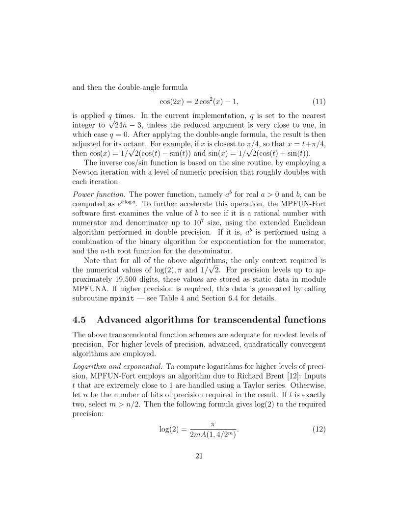
and then the double-angle formula

cos(2x) = 2 cos2(x)− 1, (11)

is applied q times. In the current implementation, q is set to the nearestinteger to

√24n − 3, unless the reduced argument is very close to one, in

which case q = 0. After applying the double-angle formula, the result is thenadjusted for its octant. For example, if x is closest to π/4, so that x = t+π/4,then cos(x) = 1/

√2(cos(t)− sin(t)) and sin(x) = 1/

√2(cos(t) + sin(t)).

The inverse cos/sin function is based on the sine routine, by employing aNewton iteration with a level of numeric precision that roughly doubles witheach iteration.

Power function. The power function, namely ab for real a > 0 and b, can becomputed as eb log a. To further accelerate this operation, the MPFUN-Fortsoftware first examines the value of b to see if it is a rational number withnumerator and denominator up to 107 size, using the extended Euclideanalgorithm performed in double precision. If it is, ab is performed using acombination of the binary algorithm for exponentiation for the numerator,and the n-th root function for the denominator.

Note that for all of the above algorithms, the only context required isthe numerical values of log(2), π and 1/

√2. For precision levels up to ap-

proximately 19,500 digits, these values are stored as static data in moduleMPFUNA. If higher precision is required, this data is generated by callingsubroutine mpinit — see Table 4 and Section 6.4 for details.

4.5 Advanced algorithms for transcendental functions

The above transcendental function schemes are adequate for modest levels ofprecision. For higher levels of precision, advanced, quadratically convergentalgorithms are employed.

Logarithm and exponential. To compute logarithms for higher levels of preci-sion, MPFUN-Fort employs an algorithm due to Richard Brent [12]: Inputst that are extremely close to 1 are handled using a Taylor series. Otherwise,let n be the number of bits of precision required in the result. If t is exactlytwo, select m > n/2. Then the following formula gives log(2) to the requiredprecision:

log(2) =π

2mA(1, 4/2m). (12)

21

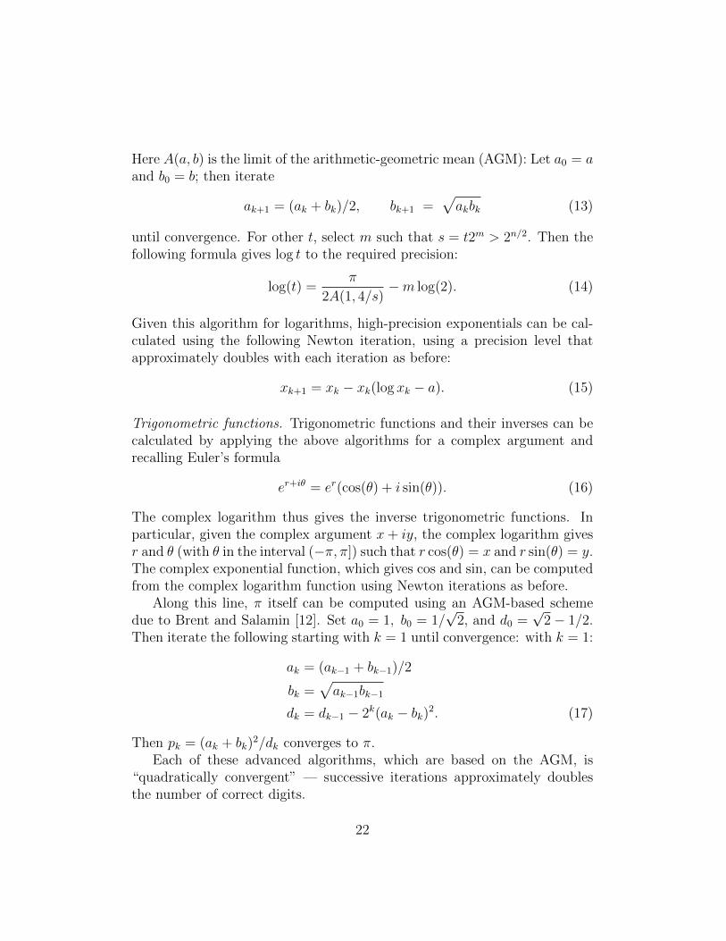
Here A(a, b) is the limit of the arithmetic-geometric mean (AGM): Let a0 = aand b0 = b; then iterate

ak+1 = (ak + bk)/2, bk+1 =√akbk (13)

until convergence. For other t, select m such that s = t2m > 2n/2. Then thefollowing formula gives log t to the required precision:

log(t) =π

2A(1, 4/s)−m log(2). (14)

Given this algorithm for logarithms, high-precision exponentials can be cal-culated using the following Newton iteration, using a precision level thatapproximately doubles with each iteration as before:

xk+1 = xk − xk(log xk − a). (15)

Trigonometric functions. Trigonometric functions and their inverses can becalculated by applying the above algorithms for a complex argument andrecalling Euler’s formula

er+iθ = er(cos(θ) + i sin(θ)). (16)

The complex logarithm thus gives the inverse trigonometric functions. Inparticular, given the complex argument x+ iy, the complex logarithm givesr and θ (with θ in the interval (−π, π]) such that r cos(θ) = x and r sin(θ) = y.The complex exponential function, which gives cos and sin, can be computedfrom the complex logarithm function using Newton iterations as before.

Along this line, π itself can be computed using an AGM-based schemedue to Brent and Salamin [12]. Set a0 = 1, b0 = 1/

√2, and d0 =

√2− 1/2.

Then iterate the following starting with k = 1 until convergence: with k = 1:

ak = (ak−1 + bk−1)/2

bk =√ak−1bk−1

dk = dk−1 − 2k(ak − bk)2. (17)

Then pk = (ak + bk)2/dk converges to π.

Each of these advanced algorithms, which are based on the AGM, is“quadratically convergent” — successive iterations approximately doublesthe number of correct digits.

22

Based on the present author’s implementation, the advanced exponen-tial function algorithm is faster than the conventional routine beginning atabout 5,800 digits. However, the advanced logarithm scheme is faster thanthe conventional logarithm after only 430 digits. Sadly, although the ad-vanced trigonometric function algorithm is not faster until above approxi-mately 1,000,000 digits, the advanced inverse trigonometric routine is fasterafter only 1,500 digits.

Note that none of these algorithms requires any context, except for thenumerical values of log 2 and π, which, as noted above, are stored in theprogram code itself for precision levels up to 19,500 digits.

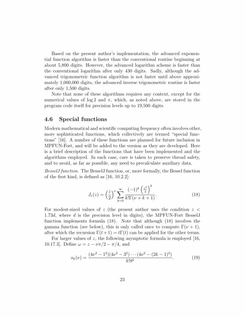
4.6 Special functions

Modern mathematical and scientific computing frequency often involves other,more sophisticated functions, which collectively are termed “special func-tions” [16]. A number of these functions are planned for future inclusion inMPFUN-Fort, and will be added to the version as they are developed. Hereis a brief description of the functions that have been implemented and thealgorithms employed. In each case, care is taken to preserve thread safety,and to avoid, as far as possible, any need to precalculate auxiliary data.

BesselJ function. The BesselJ function, or, more formally, the Bessel functionof the first kind, is defined as [16, 10.2.2]:

Jν(z) =(z

2

)ν ∞∑k=0

(−1)k(z2

4

)kk!Γ(ν + k + 1)

. (18)

For modest-sized values of z (the present author uses the condition z <1.73d, where d is the precision level in digits), the MPFUN-Fort BesselJfunction implements formula (18). Note that although (18) involves thegamma function (see below), this is only called once to compute Γ(ν + 1),after which the recursion Γ(t+ 1) = tΓ(t) can be applied for the other terms.

For larger values of z, the following asymptotic formula is employed [16,10.17.3]. Define ω = z − νπ/2− π/4, and

ak(ν) =(4ν2 − 12)(4ν2 − 32) · · · (4ν2 − (2k − 1)2)

k!8k. (19)

23

Then

Jν(z) =

(2

πz

)1/2(

cosω∞∑k=0

(−1)ka2k(ν)

z2k− sinω

∞∑k=0

(−1)ka2k+1(ν)

z2k+1

).

(20)

One important detail omitted from the above discussion is that largeamounts of cancellation occurs in these formulas. Thus when evaluating theseformulas, a working precision of 1.5 times the normal working precision isemployed.

No precalculated auxiliary data is needed for either of these algorithms,so they are thread safe.

Gamma function. The gamma function employs a very efficient but little-known formula due to Ronald W. Potter [25], as follows. If the input t is apositive integer, then Γ(t) = (t−1)!. If not, use the recursion Γ(t+1) = tΓ(t)to reduce the argument (positive or negative) to the interval (0, 1). Thendefine α = nint (n/2 · log 2), where n is the number of bits of precision andnint means nearest integer, and set z = α2/4. Define the Pochhammerfunction as

(ν)k = ν(ν + 1)(ν + 2) · · · (ν + k − 1). (21)

Then define the functions

A(ν, z) =(z

2

)νν∞∑k=0

(z2/4)k

k!(ν)k+1

B(ν, z) =(z

2

)−ν(−ν)

∞∑k=0

(z2/4)k

k!(−ν)k+1

. (22)

With these definitions, the gamma function can then be computed as

Γ(ν) =

√A(ν, z)

B(ν, z)

π

ν sin(πν). (23)

No auxiliary data is needed for this algorithm, so it is thread-safe.

Incomplete gamma function. For modest-sized positive arguments (the au-thor uses the condition z < 2.768d, where d is the precision level in digits),

24

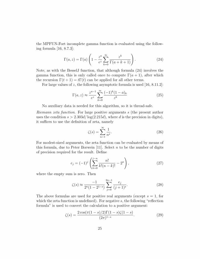
the MPFUN-Fort incomplete gamma function is evaluated using the follow-ing formula [16, 8.7.3]:

Γ(a, z) = Γ(a)

(1− za

ez

∞∑k=0

zk

Γ(a+ k + 1)

). (24)

Note, as with the BesselJ function, that although formula (24) involves thegamma function, this is only called once to compute Γ(a + 1), after whichthe recursion Γ(t+ 1) = tΓ(t) can be applied for all other terms.

For large values of z, the following asymptotic formula is used [16, 8.11.2]:

Γ(a, z) ≈ za−1

ez

∞∑k=0

(−1)k(1− a)kzk

(25)

No auxiliary data is needed for this algorithm, so it is thread-safe.

Riemann zeta function. For large positive arguments s (the present authoruses the condition s > 2.303d/ log(2.215d), where d is the precision in digits),it suffices to use the definition of zeta, namely

ζ(s) =∞∑n=1

1

ns. (26)

For modest-sized arguments, the zeta function can be evaluated by means ofthis formula, due to Peter Borwein [11]. Select n to be the number of digitsof precision required for the result. Define

ej = (−1)j

(j−n∑k=0

n!

k!(n− k)!− 2n

), (27)

where the empty sum is zero. Then

ζ(s) ≈ −1

2n(1− 21−s)

2n−1∑j=0

ej(j + 1)s

. (28)

The above formulas are used for positive real arguments (except s = 1, forwhich the zeta function is undefined). For negative s, the following “reflectionformula” is used to convert the calculation to a positive argument:

ζ(s) =2 cos(π(1− s)/2)Γ(1− s)ζ(1− s)

(2π)1−s. (29)

25

Formulas (27), (28) and (29) are implemented as the zeta function. Noauxiliary data for this algorithm required, so it is thread-safe.

A even faster algorithm, based on the Euler-Maclaurin summation for-mula, can be derived from the following [16, 25.2.9]: Select an integer pa-rameter N > 0 (the present author uses N = 0.6d, where d is the number ofdigits of precision). Then

ζ(s) ≈N∑k=1

1

ks+

1

(s− 1)N s−1 −1

2N s+∞∑k=1

(s+ 2k − 2

2k − 1

)B2k

2kN s−1+2k, (30)

where B2k are the even Bernoulli numbers

B2k =(−1)k−12(2k)!ζ(2k)

(2π)2k. (31)

Since the zeta function evaluations in (31) are for positive even integer ar-guments, they can be calculated quickly using (28). Once the requisite evenBernoulli numbers B2k (up to index k approximately matching the precisionlevel in digits) are computed, the function that implements formula (30) isthread-safe.

5 Installation, compilation and linking

Installation, compilation and linking is relatively straightforward, providedthat you have a Unix-based system, such as Linux or Apple OSX, with acommand-line interface (such as the Terminal application of Apple OSX).For Apple OSX systems, you first must install the “Command Line Tools”package, which is available (for free) from the Apple Developer website. In-structions for doing this are provided in the README.txt file in the distri-bution package for either MPFUN-Fort or MPFUN-MPFR.

To install the MPFUN-MPFR version, you must first install the GMP andMPFR packages. The latest versions are available from https://gmplib.org

and http://www.mpfr.org/mpfr-current/, respectively. Instructions forinstalling GMP and MPFR are included in the README.txt file for MPFUN-MPFR.

The gfortran compiler, which is highly recommended for either version ofMPFUN2015, is available (for free) for a variety of systems at the websitehttps://gcc.gnu.org/wiki/GFortranBinaries.

26

The MPFUN-Fort version also works with IBM’s xlf compiler, Intel’sifort and Portland Group’s pgf90. The MPFUN-MPFR version also workswith Intel’s ifort (it has not yet been tested on the other two). Compile-linkscripts for each supported compiler are provided in the distribution softwaredirectory.

Each version of the software comes in two variants:

• Variant 1: This is recommended for basic applications that do notdynamically change the precision level (or do so only rarely).

• Variant 2: This is recommended for more sophisticated applicationsthat dynamically change the precision level (see Section 6.4 below).

As an example, if one has installed the GNU gfortran compiler, thenvariant 1 can be compiled by typing

./gnu-complib1.scr

Then the application program progx.f90 can be compiled and linked withvariant 1 of the library, producing the executable progx, by typing

./gnu-complink1.scr progx

These scripts assume that the user program is in the same directory as thelibrary files; this can easily be changed by editing the script files.

6 Fortran coding instructions

A high-level Fortran interface is provided for both versions of the package.A C++ interface is planned but not complete.

As mentioned above, to use either version of the MPFUN2015 package,the user first sets the parameter mpipl, the “default” precision level in digits,which is the maximum precision level to be used for subsequent computation,and is used to specify the amount of storage required for multiprecision data.mpipl is set in a parameter statement at the start of module MPFUNF, whichis in file mpfunf.f90. In the code as distributed, mpipl is set to 1200 digits(sufficient to run the six test programs of Section 7), but it can be set to anylevel greater than or equal to 30 digits. mpipl is automatically converted tomantissa words by the formula mpwds = int (mpipl / mpdpw + 2), wherempdpw is a system parameter, and where int () means truncate to integer.For MPFUN-Fort, mpdpw is log10(2

48) = 14.44943979187 . . . , whereas forMPFUN-MPFR it is log10(2

64) = 19.26591972249 . . . (both values are double

27

precision approximations). The resulting parameter mpwds is the internaldefault precision level, in words. All computations are performed to mpwds

words precision unless the user, in an application code, specifies a lower value.After setting the value of mpipl in module MPFUNF, compile either

variant 1 or variant 2 of the library, using one of the scripts mentioned above.Next, place the following line in every subprogram of the user’s applica-

tion code that contains a multiprecision variable or array, at the beginningof the declaration section, before any implicit or type statements:

use mpmodule

To designate a variable or array as multiprecision real (MPR) in an applica-tion program, use a Fortran-90 type statement with the type mp real, as inthis example:

type (mp real) a, b(m), c(m,n)

Similarly, to designate a variable or array as multiprecision complex (MPC),use a type statement with the type mp complex. Thereafter when one ofthese variables or arrays appears, as in the code

d = a + b(i) * sqrt(3.d0 - c(i,j))

the proper underlying multiprecision routines are automatically called.Most common mixed-mode combinations (arithmetic operations, compar-

isons and assignments) involving MPR, MPC, double precision (DP), doublecomplex (DC), and integer operands are supported. A complete list of sup-ported mixed-mode operations is given in Table 2. See Section 6.3 belowabout DP and DC constants and expressions.

Input/output of MP variables or array elements is done using specialsubroutines. See Table 6.1 and Section 6.2 for details.

In the MPFUN-Fort version, the above instructions apply if the precisionlevel, namely mpipl, is 19,500 digits or less. For higher precision, in additionto changing mpipl to this higher level, one must call mpinit at the startof execution, before any multiprecision computation is done. If this is amultithreaded application, this initialization must be done in single-threadedmode. With variant 1, subroutine mpinit has an optional argument, which isthe maximum precision level, in words; if not present, the default precision,namely mpwds words (which corresponds to mpipl digits), is assumed. Invariant 2, this argument is required. See Section 6.4 for details. When theinitialization feature of MPFR is available, this same call will apply to theMPFUN-MPFR version.

28

Operator Arg 1 Arg 2 Operator Arg 1 Arg 2

a = b MPR MPR +, -, *, / MPR MPR(assignment) DP MPR (+,−,×,÷) DP MPR

Int MPR MPR DPMPR MPC Int MPRMPC MPR MPR IntMPC MPC MPC MPCDP MPC DP MPCDC MPC MPC DPMPR DP [1] DC MPCMPR Int [1] MPC DCMPR Char [1] MPR MPCMPC DP [1] MPC MPRMPC DC [1]

a**b MPR Int ==, /= MPR MPR(ab) MPR MPR (=, 6= tests) DP MPR

MPC Int MPR DPMPC MPC Int MPRMPR MPC MPR IntMPC MPR MPC MPC

<=, >=, <, > MPR MPR DP MPC(≤,≥, <,> tests) DP MPR MPC DP

MPR DP DC MPCInt MPR MPC DCMPR Int MPR MPC

MPC MPR

Table 2: Supported mixed-mode operator combinations. MPR denotes mul-tiprecision real, MPC denotes multiprecision complex, DP denotes doubleprecision, DC denotes double complex, Int denotes integer and Char denotesarbitrary-length character string. Note:[1] These operations are not allowed in variant 2 — see Section 6.4.

29

Note in particular that for the time being, computations performed usingthe MPFUN-MPFR version that involve transcendental functions are notthread-safe, unless one has built the MPFR library with the thread-safe buildoption. This limitation will be removed in a future release of the package.

6.1 Functions and subroutines

Most Fortran-2008 intrinsic functions [18] are supported in MPFUN2015 withMPR and MPC arguments, as appropriate. A full listing of these functionsis shown in Table 3. In each case, these functions represent a straightforwardextension to MPR or MPC arguments, as indicated. Tables 4 and 5 presenta list of additional functions and subroutines provided in this package. Inthese tables, “F” denotes function, “S” denotes subroutine, “MPR” denotesmultiprecision real, “MPC” denotes multiprecision complex, “DP” denotesdouble precision, “DC” denotes double complex, “Int” denotes integer and“Q” denotes IEEE quad precision (i.e., real*16), if supported. The variablenames r1,r2,r3 are MPR, z1 is MPC, d1 is DP, dc1 is DC, i1,i2,i3 areintegers, s1 is character*1, sn is character*n for any n, and rr is MPR oflength i1.

6.2 Input and output of multiprecision data

Binary-decimal conversion and input or output of multiprecision data is nothandled by standard Fortran read/write commands, but instead is handledby special subroutines, as briefly mentioned in Table 4. Here are the details:

1. subroutine mpeform (r1,i1,i2,s1). This converts the MPR num-ber r1 into character form in the character*1 array s1. The argumenti1 (input) is the length of the output string, and i2 (input) is thenumber of digits after the decimal point. The format is analogous toFortran E format. The result is left-justified among the i1 cells of s1.The condition i1 ≥ i2 +20 must hold.

2. subroutine mpfform (r1,i1,i2,s1). This converts the MPR num-ber r1 into character form in the character*1 array s1. The argumenti1 (input) is the length of the output string, and i2 (input) is thenumber of digits after the decimal point. The format is analogous toFortran F format. The result is right-justified among the i1 cells of s1.The condition i1 ≥ i2 +10 must hold.

30

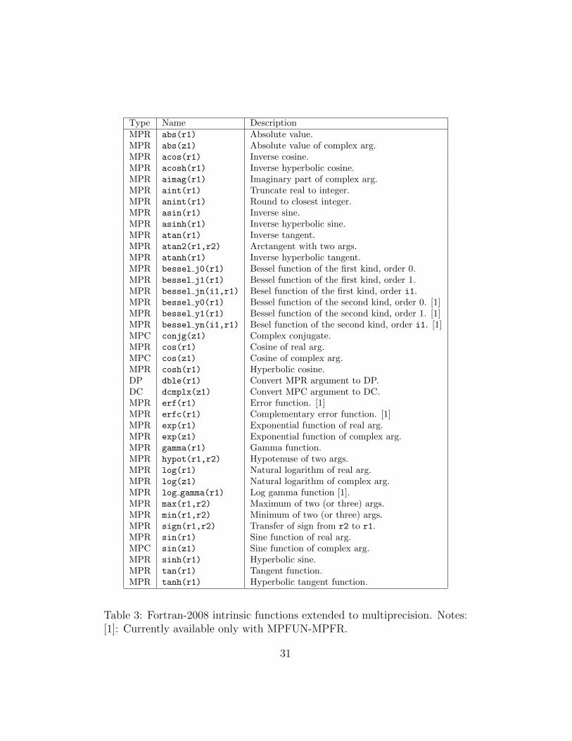
Type Name DescriptionMPR abs(r1) Absolute value.MPR abs(z1) Absolute value of complex arg.MPR acos(r1) Inverse cosine.MPR acosh(r1) Inverse hyperbolic cosine.MPR aimag(r1) Imaginary part of complex arg.MPR aint(r1) Truncate real to integer.MPR anint(r1) Round to closest integer.MPR asin(r1) Inverse sine.MPR asinh(r1) Inverse hyperbolic sine.MPR atan(r1) Inverse tangent.MPR atan2(r1,r2) Arctangent with two args.MPR atanh(r1) Inverse hyperbolic tangent.MPR bessel j0(r1) Bessel function of the first kind, order 0.MPR bessel j1(r1) Bessel function of the first kind, order 1.MPR bessel jn(i1,r1) Besel function of the first kind, order i1.MPR bessel y0(r1) Bessel function of the second kind, order 0. [1]MPR bessel y1(r1) Bessel function of the second kind, order 1. [1]MPR bessel yn(i1,r1) Besel function of the second kind, order i1. [1]MPC conjg(z1) Complex conjugate.MPR cos(r1) Cosine of real arg.MPC cos(z1) Cosine of complex arg.MPR cosh(r1) Hyperbolic cosine.DP dble(r1) Convert MPR argument to DP.DC dcmplx(z1) Convert MPC argument to DC.MPR erf(r1) Error function. [1]MPR erfc(r1) Complementary error function. [1]MPR exp(r1) Exponential function of real arg.MPR exp(z1) Exponential function of complex arg.MPR gamma(r1) Gamma function.MPR hypot(r1,r2) Hypotenuse of two args.MPR log(r1) Natural logarithm of real arg.MPR log(z1) Natural logarithm of complex arg.MPR log gamma(r1) Log gamma function [1].MPR max(r1,r2) Maximum of two (or three) args.MPR min(r1,r2) Minimum of two (or three) args.MPR sign(r1,r2) Transfer of sign from r2 to r1.MPR sin(r1) Sine function of real arg.MPC sin(z1) Sine function of complex arg.MPR sinh(r1) Hyperbolic sine.MPR tan(r1) Tangent function.MPR tanh(r1) Hyperbolic tangent function.

Table 3: Fortran-2008 intrinsic functions extended to multiprecision. Notes:[1]: Currently available only with MPFUN-MPFR.

31

Type Name DescriptionF(MPC) mpcmplx(r1,r2) Converts (r1,r2) to MPC. [1]F(MPC) mpcmplx(dc1) Converts DC arg to MPC. [1]F(MPC) mpcmplx(z1) Converts MPC arg to MPC. [1]F(MPC) mpcmplxdc(dc1) Converts DC to MPC, without checking. [1, 2]S mpcssh(r1,r2,r3) Returns both cosh and sinh of r1, in the same

time as calling just cosh or just sinh.S mpcssn(r1,r2,r3) Returns both cos and sin of r1, in the same

time as calling just cos or just sin.S mpeform(r1,i1,i2,s1) Converts r1 to char*1 string in Ei1.i2

format, suitable for output (Sec. 6.2).S mpfform(r1,i1,i2,s1) Converts r1 to char*1 string in Fi1.i2

format, suitable for output (Sec. 6.2).F(MPR) mpegamma() Returns Euler’s γ constant. [1, 3]S mpinit Initializes for extra-high precision (Sec. 6). [1]F(MPR) mplog2() Returns log(2). [1]F(MPR) mpnrt(r1,i1) Returns the i1-th root of r1.F(MPR) mppi() Returns π. [1]F(MPR) mpprodd(r1,d1) Returns r1*d1, without checking. [2]F(MPR) mpquotd(r1, d1) Returns r1/d1, without checking. [2]S mpread(i1,r1) Inputs r1 from Fortran unit i1; up to five

MPR args may be listed (Sec. 6.2). [1]S mpread(i1,z1) Inputs z1 from Fortran unit i1; up to five

MPC args may be listed (Sec. 6.2). [1]F(MPR) mpreal(r1) Converts MPR arg to MPR. [1]F(MPR) mpreal(z1) Converts MPC arg to MPR. [1]F(MPR) mpreal(d1) Converts DP arg to MPR. [1, 2]F(MPR) mpreal(q1) Converts real*16 to MPR. [1, 2]F(MPR) mpreal(s1,i1) Converts char*1 string to MPR (Sec. 6.2). [1]F(MPR) mpreal(sn) Converts char*n string to MPR (Sec. 6.2). [1]F(MPR) mpreald(d1) Converts DP to MPR, without checking. [1, 2]F(Int) mpwprec(r1) Returns precision in words assigned to r1.F(Int) mpwprec(z1) Returns precision in words assigned to z1.S mpwrite(i1,i2,i3,r1) Outputs r1 in Ei2.i3 format to unit i1; up to

five MPR args may be listed (Sec. 6.2).S mpwrite(i1,i2,i3,z1) Outputs z1 in Ei2.i3 format to unit i1; up to

five MPC args may be listed (Sec. 6.2) .F(Q) qreal(r1) Converts MPR to real*16.

Table 4: Additional general routines (F: function, S: subroutine). Notes:[1]: In variant 1, an integer precision level argument (mantissa words) mayoptionally be added as the final argument; this argument is required in vari-ant 2. See Section 6.4.[2]: These do not check DP or DC values. See Section 6.3.[3]: These are currently only available with MPFUN-MPFR.

32

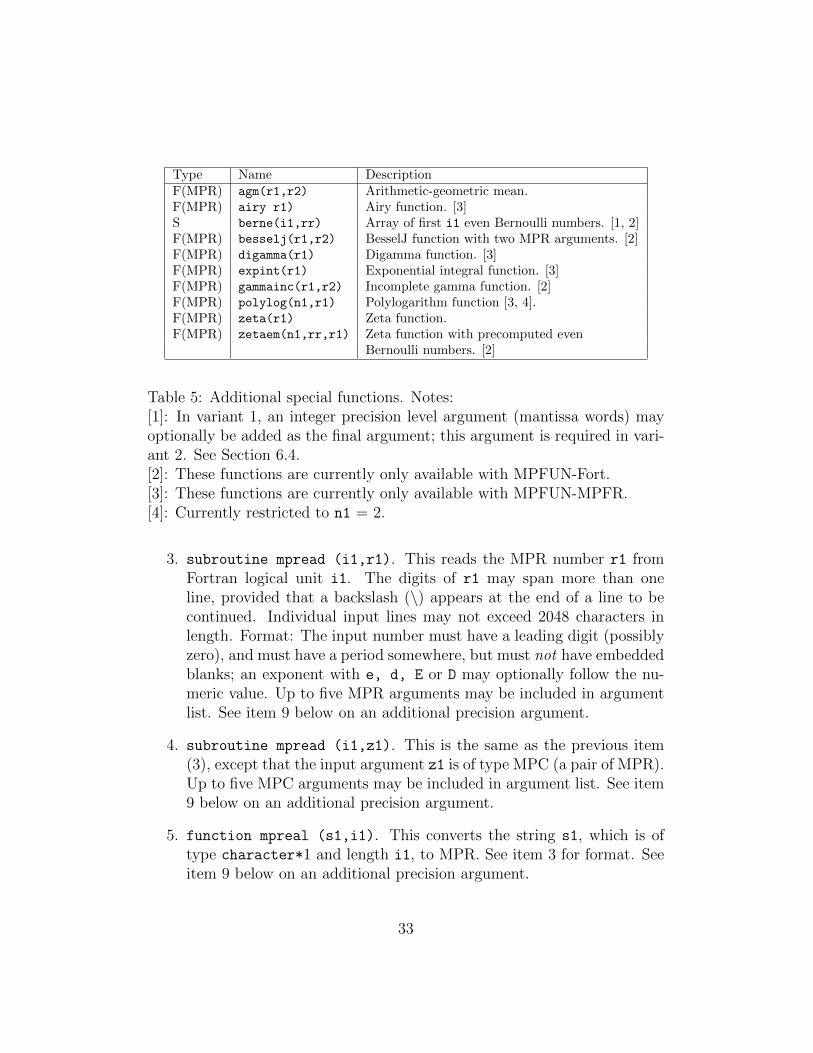
Type Name DescriptionF(MPR) agm(r1,r2) Arithmetic-geometric mean.F(MPR) airy r1) Airy function. [3]S berne(i1,rr) Array of first i1 even Bernoulli numbers. [1, 2]F(MPR) besselj(r1,r2) BesselJ function with two MPR arguments. [2]F(MPR) digamma(r1) Digamma function. [3]F(MPR) expint(r1) Exponential integral function. [3]F(MPR) gammainc(r1,r2) Incomplete gamma function. [2]F(MPR) polylog(n1,r1) Polylogarithm function [3, 4].F(MPR) zeta(r1) Zeta function.F(MPR) zetaem(n1,rr,r1) Zeta function with precomputed even

Bernoulli numbers. [2]

Table 5: Additional special functions. Notes:[1]: In variant 1, an integer precision level argument (mantissa words) mayoptionally be added as the final argument; this argument is required in vari-ant 2. See Section 6.4.[2]: These functions are currently only available with MPFUN-Fort.[3]: These functions are currently only available with MPFUN-MPFR.[4]: Currently restricted to n1 = 2.

3. subroutine mpread (i1,r1). This reads the MPR number r1 fromFortran logical unit i1. The digits of r1 may span more than oneline, provided that a backslash (\) appears at the end of a line to becontinued. Individual input lines may not exceed 2048 characters inlength. Format: The input number must have a leading digit (possiblyzero), and must have a period somewhere, but must not have embeddedblanks; an exponent with e, d, E or D may optionally follow the nu-meric value. Up to five MPR arguments may be included in argumentlist. See item 9 below on an additional precision argument.

4. subroutine mpread (i1,z1). This is the same as the previous item(3), except that the input argument z1 is of type MPC (a pair of MPR).Up to five MPC arguments may be included in argument list. See item9 below on an additional precision argument.

5. function mpreal (s1,i1). This converts the string s1, which is oftype character*1 and length i1, to MPR. See item 3 for format. Seeitem 9 below on an additional precision argument.

33

6. function mpreal (sn). This converts the string sn, which may be oftype character*n for any n, to MPR. See item 3 for format. On somesystems, n may be limited, say to 2048; if this is a problem, use previousitem (5). See item 9 below on an additional precision argument.

7. subroutine mpwrite (i1,i2,i3,r1). This writes the MPR numberr1 to Fortran logical unit i1. The argument i2 (input) is the lengthof the output field, and i3 (input) is the number of digits after thedecimal point. The format is analogous to Fortran E format and isleft-justified in the field. Up to five MPR arguments may be includedin argument list.

8. subroutine mpwrite (i1,i2,i3,z1). This is the same as the previ-ous item (7), except that the argument z1 is of type MPC (a pair ofMPR). Up to five MPC arguments may be included in argument list.

9. Note: For mpread (items 3 and 4) and mpreal (items 5 and 6), whenusing variant 1, an integer precision level argument (mantissa words)may optionally be added as the final argument; this argument is re-quired in variant 2. See Section 6.4.

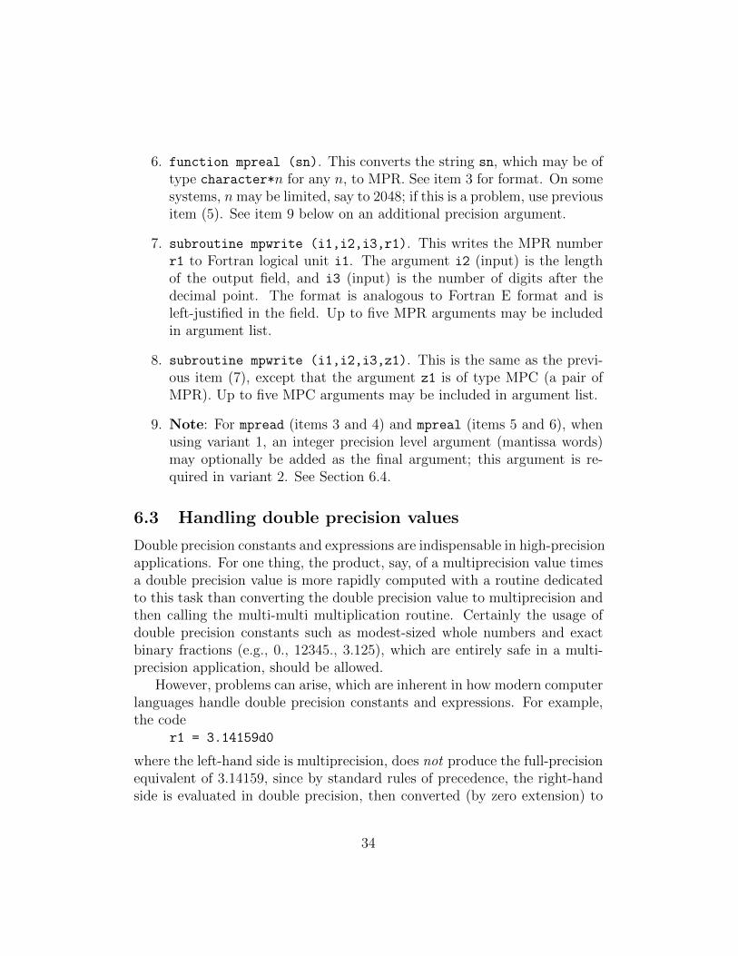
6.3 Handling double precision values

Double precision constants and expressions are indispensable in high-precisionapplications. For one thing, the product, say, of a multiprecision value timesa double precision value is more rapidly computed with a routine dedicatedto this task than converting the double precision value to multiprecision andthen calling the multi-multi multiplication routine. Certainly the usage ofdouble precision constants such as modest-sized whole numbers and exactbinary fractions (e.g., 0., 12345., 3.125), which are entirely safe in a multi-precision application, should be allowed.

However, problems can arise, which are inherent in how modern computerlanguages handle double precision constants and expressions. For example,the code

r1 = 3.14159d0

where the left-hand side is multiprecision, does not produce the full-precisionequivalent of 3.14159, since by standard rules of precedence, the right-handside is evaluated in double precision, then converted (by zero extension) to

34

the left-hand side. When using the package, one can avoid this problem bywriting this as

r1 = ’3.14159’

By enclosing the constant in apostrophes (and changing it to a literal), thisindicates to the MPFUN2015 software that the constant is to be evaluatedto full precision.

A closely related problem is the following: The coder2 = r1 + 3.d0 * sqrt (2.d0)

does not produce a fully accurate result, since the subexpression 3.d0 *

sqrt (2.d0) is performed in double precision (again, according to standardrules of operator precedence in all major programming languages). The so-lution here is to write this as

r2 = r1 + 3.d0 * sqrt (mpreal (2.d0))

or, if using variant 2, asr2 = r1 + 3.d0 * sqrt (mpreal (2.d0, nwds))

where nwds is the precision level, in words, to be assigned to the constant 2

(see Section 6.4). This forces all operations to be done using MP routines.To help avoid such problems, the MPFUN2015 low-level software checks

every double precision value (constants, variables and expression values) ina multiprecision statement at execution time to see if it has more than 40significant bits. If so, it is flagged as an error, since very likely such usagerepresents an unintended loss of precision in the application program. Thisfeature catches 99.99% of accuracy loss problems due to the usage of inexactdouble precision values.

On the other hand, some applications contain legitimate double preci-sion constants that are trapped by this test. For example, in the tpslqm2and tpslqm3 programs listed in Section 7, exact double precision values canarise that are greater than 40 bits in size. In order to permit such usage,four special functions have been provided: mpprodd, mpquotd, mpreald,

mpcmplxdc (see Table 4). The first and second return the product and quo-tient, respectively, of a MPR argument and a DP argument; the third con-verts a DP value to MPR (with an optional precision level parameter — seeSection 6.4); and the fourth converts a DC value to MPC (with an optionalprecision level parameter — see Section 6.4). These routines do not checkthe double precision argument to see if it has more than 40 significant bits.

35

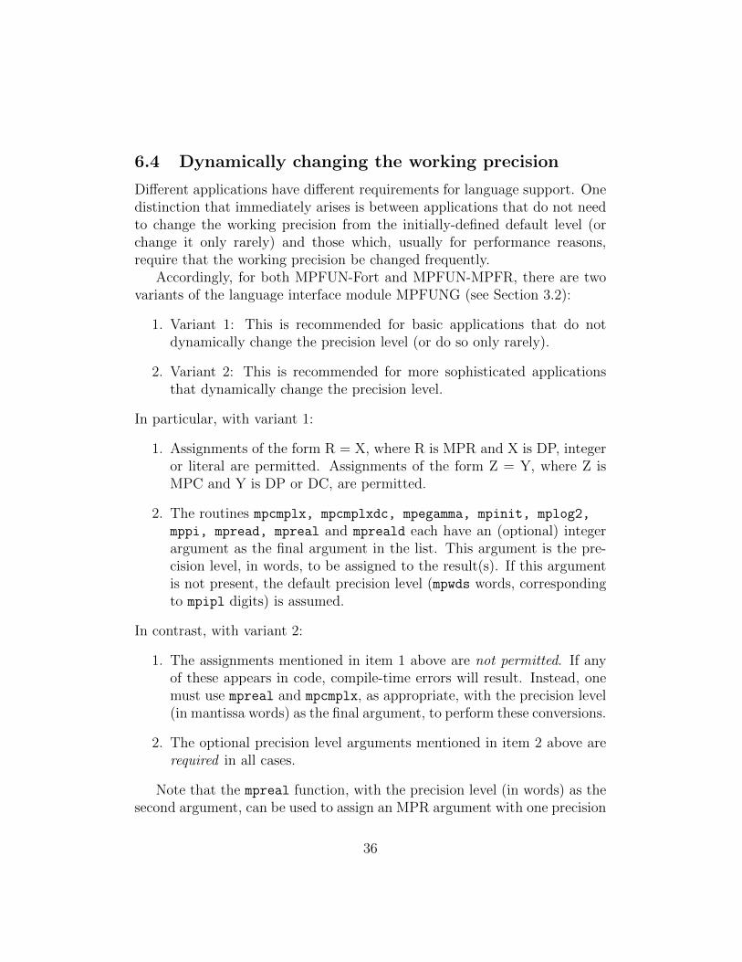
6.4 Dynamically changing the working precision

Different applications have different requirements for language support. Onedistinction that immediately arises is between applications that do not needto change the working precision from the initially-defined default level (orchange it only rarely) and those which, usually for performance reasons,require that the working precision be changed frequently.

Accordingly, for both MPFUN-Fort and MPFUN-MPFR, there are twovariants of the language interface module MPFUNG (see Section 3.2):

1. Variant 1: This is recommended for basic applications that do notdynamically change the precision level (or do so only rarely).

2. Variant 2: This is recommended for more sophisticated applicationsthat dynamically change the precision level.

In particular, with variant 1:

1. Assignments of the form R = X, where R is MPR and X is DP, integeror literal are permitted. Assignments of the form Z = Y, where Z isMPC and Y is DP or DC, are permitted.

2. The routines mpcmplx, mpcmplxdc, mpegamma, mpinit, mplog2,

mppi, mpread, mpreal and mpreald each have an (optional) integerargument as the final argument in the list. This argument is the pre-cision level, in words, to be assigned to the result(s). If this argumentis not present, the default precision level (mpwds words, correspondingto mpipl digits) is assumed.

In contrast, with variant 2:

1. The assignments mentioned in item 1 above are not permitted. If anyof these appears in code, compile-time errors will result. Instead, onemust use mpreal and mpcmplx, as appropriate, with the precision level(in mantissa words) as the final argument, to perform these conversions.

2. The optional precision level arguments mentioned in item 2 above arerequired in all cases.

Note that the mpreal function, with the precision level (in words) as thesecond argument, can be used to assign an MPR argument with one precision

36

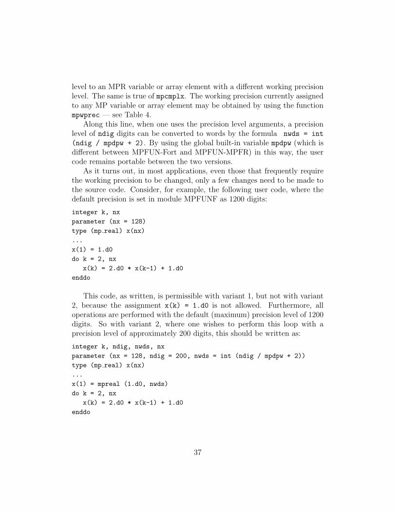
level to an MPR variable or array element with a different working precisionlevel. The same is true of mpcmplx. The working precision currently assignedto any MP variable or array element may be obtained by using the functionmpwprec — see Table 4.

Along this line, when one uses the precision level arguments, a precisionlevel of ndig digits can be converted to words by the formula nwds = int

(ndig / mpdpw + 2). By using the global built-in variable mpdpw (which isdifferent between MPFUN-Fort and MPFUN-MPFR) in this way, the usercode remains portable between the two versions.

As it turns out, in most applications, even those that frequently requirethe working precision to be changed, only a few changes need to be made tothe source code. Consider, for example, the following user code, where thedefault precision is set in module MPFUNF as 1200 digits:

integer k, nx

parameter (nx = 128)

type (mp real) x(nx)

...

x(1) = 1.d0

do k = 2, nx

x(k) = 2.d0 * x(k-1) + 1.d0

enddo

This code, as written, is permissible with variant 1, but not with variant2, because the assignment x(k) = 1.d0 is not allowed. Furthermore, alloperations are performed with the default (maximum) precision level of 1200digits. So with variant 2, where one wishes to perform this loop with aprecision level of approximately 200 digits, this should be written as:

integer k, ndig, nwds, nx

parameter (nx = 128, ndig = 200, nwds = int (ndig / mpdpw + 2))

type (mp real) x(nx)

...

x(1) = mpreal (1.d0, nwds)

do k = 2, nx

x(k) = 2.d0 * x(k-1) + 1.d0

enddo

37

Note that by changing x(1) = 1.d0 to x(1) = mpreal (1.d0, nwds),the array element x(1) is assigned the value 1.0, with a working precision ofnwds words (i.e., 200 digits). In the loop, when k is 2, x(2) also inherits theworking precision level nwds words, since it is computed with an expressionthat involves x(1). By induction, all elements of the array x inherit theworking precision level nwds words (i.e., 200 digits).

This scenario is entirely typical of other types of algorithms and applica-tions — in most cases, it is only necessary to make a few code changes, suchas in assignments to double precision values before a loop, to completely con-trol dynamic precision. It is recommended, though, that the user employ thesystem function mpwprec, which returns the working precision level currentlyassigned to an input multiprecision variable or array element (see Table 4),to ensure that the precision level the user thinks is assigned to a variable isindeed the level being used by the program.

Using variant 2, with its stricter coding standards, requires a bit moreprogramming effort, but in the present author’s experience, when dealingwith applications that dynamically change the precision level, this additionaleffort is more than repaid by fewer debugging and performance problems inactual usage. A code written for variant 2 also works with variant 1, but notvice versa. See the sample test codes mentioned in the next section, all ofwhich are written to conform to the standards of variant 2.

7 Performance of sample applications

Numerous full-scale multiprecision applications have been implemented usingthe MPFUN2015 software, including some that dynamically vary the workingprecision level. In most cases, only very minor modifications needed to bemade to existing double precision source code. Some examples include thefollowing:

1. tpslq1: A one-level standard PSLQ program; finds the coefficients ofthe degree-30 polynomial satisfied by 31/5 − 21/6. Size of code: 752lines. Precision level: 240 digits.

2. tpslqm1: A one-level multipair PSLQ program; finds the coefficientsof the degree-30 polynomial satisfied by 31/5 − 21/6. Size of code: 905lines. Precision level: 240 digits.

38

3. tpslqm2: A two-level multipair PSLQ program; finds the coefficientsof the degree-56 polynomial satisfied by 31/7 − 21/8. Size of code: 1694lines. Precision level: 640 digits; switches frequently between multi-precision and double precision.

4. tpslqm3: A three-level multipair PSLQ program; finds the coefficientsof the degree-72 polynomial satisfied by 31/8 − 21/9. Size of code: 2076lines. Precision level: 1100 digits; switches frequently between fullprecision, medium precision (120 digits) and double precision.

5. tquad: A quadrature program; performs the tanh-sinh, the exp-sinhor the sinh-sinh quadrature algorithm, as appropriate, on a suite of 18problems involving numerous transcendental function references, pro-ducing results correct to 500-digit accuracy. Size of code: 1421 lines.Precision level: 1000 digits, but most computation is done to 500 digits;switches frequently between 500 and 1000 digits.

6. tpphix3: A Poisson phi program; computes the value of φ2(x, y) andthen employs a three-level multipair PSLQ algorithm to find the mini-mal polynomial of degree m satisfied by exp(8πφ2(1/k, 1/k)) for a givenk (see Section 1.4). In the code as distributed, k = 30, m = 64, anda palindromic option is employed so that the multipair PSLQ routines(which are part of this application) searches for a relation of size 33instead of 65. This computation involves transcendental functions andboth real and complex multiprecision arithmetic. Size of code: 2506lines. Precision level: 1100 digits; switches frequently between full pre-cision, medium precision (160 digits) and double precision.

Each of the above six programs, with a reference output file for compar-ison, is included in the software’s distribution package. These codes workidentically with both the MPFUN-Fort and the MPFUN-MPFR versions —no changes are required to switch from one version to the other. The scriptmpfun-tests.scr, which is included in the distribution package for each ver-sion, compiles variant 2 of the library, then compiles, links and runs all sixof the test programs, plus a brief validity check program.

If, after running the test script, the results reproduce the results in thereference output files (except possibly the CPU run times and the iterationcounts in the PSLQ runs), then one can be fairly confident that the software isworking properly. Note that the final output relation of the PSLQ runs might

39

have all signs reversed from the reference output (which is mathematicallyequivalent).

These programs are provided, in part, as examples of programming tech-niques when using the MPFUN2015 package. Users may feel free to adaptthese codes, although the present author would appreciate being notified andcredited when this is done. All application programs and library codes arepublicly available but are subject to copyright and other legal conditions.For details, see the file disclaimer.txt in the distribution package.

7.1 Timings

Table 6 presents some performance timings comparing the two versions of thepackage, and for the GNU gfortran and Intel ifort compilers. Note that withthe MPFUN-MPFR version, the GNU C compiler was used to build the GMPand MPFR libraries, no matter what compiler was employed to compile theMPFUN-MPFR libraries and the application code. These runs were made ona 2.9 GHz MacBook Pro with an Intel Core i5 processor and 8 Gbyte of mainmemory. For uniformity, the timings are listed in the Table 6 to two decimalplace accuracy, but, as with all computer run time measurements, they shouldnot be considered repeatable beyond about two or three significant digits.

The tested codes include the first six applications listed in the previoussection, and, in addition, the Poisson phi program, which is performed for arange of problem sizes without the palindromic option.

Examining these results, and focusing on the longer-running programs inthe suite, we observe a roughly 3X performance advantage for the MPFUN-MPFR version over the MPFUN-Fort version, and a roughly 25% perfor-mance advantage for the Intel ifort compiler over the GNU gfortran com-piler. Note that for the programs tquadts and tquadtsp, which perform nu-merical integration using tanh-sinh quadrature, MPFUN-MPFR is roughlynine times faster, with either compiler, than MPFUN-Fort. This reflects thevery fast performance of transcendental functions in MPFR. For the otherapplications, which are dominated by algebraic operations, the ratio is lower.

8 Conclusion

The current version of the software and documentation is available at:http://www.davidhbailey.com/dhbsoftware

40

tpphix3 GNU gfortran Intel ifortPrecision param. MPFUN- MPFUN- MPFUN- MPFUN-

Code name (digits) k m Fort MPFR Fort MPFR

tpslq1 240 16.45 4.33 11.22 4.03tpslqm1 240 13.91 2.94 4.63 2.61tpslqm2 650 15.96 7.97 11.94 5.78tpslqm3 1100 69.52 32.47 39.76 26.96tquad 1000 76.07 7.59 76.83 7.48tpphix3 700 18 36 7.34 2.63 3.72 2.18tpphix3 2000 22 60 93.39 35.93 65.82 30.75tpphix3 2100 17 64 144.91 52.05 89.94 43.91tpphix3 2700 26 72 261.50 94.55 185.31 80.18tpphix3 5000 25 100 2023.77 663.69 1423.03 501.51tpphix3 8200 32 128 9704.11 3239.61 7318.59 2221.86

Table 6: Timings on a suite of test programs (seconds).

41

References

[1] D. H. Bailey and J. M. Borwein, “High-precision arithmetic inmathematical physics,” Mathematics, vol. 3 (2015), pg. 337–367.http://www.mdpi.com/2227-7390/3/2/337/pdf.

[2] D. H. Bailey, X. S. Li and K. Jeyabalan, “A comparison of threehigh-precision quadrature schemes,” Experimental Mathematics, vol.14 (2005), no. 3, pg. 317–329.

[3] D. H. Bailey, R. Barrio, and J. M. Borwein, “High precisioncomputation: Mathematical physics and dynamics,” AppliedMathematics and Computation, vol. 218 (2012), pg. 10106-10121.

[4] D. H. Bailey and J. M. Borwein, “Hand-to-hand combat withthousand-digit integrals,” Journal of Computational Science, vol. 3(2012), pg. 77-86.

[5] D. H. Bailey, J. M. Borwein, R. E. Crandall and J. Zucker, “Latticesums arising from the Poisson equation,” Journal of Physics A:Mathematical and Theoretical, vol. 46 (2013), pg. 115201,http://www.davidhbailey.com/dhbpapers/PoissonLattice.pdf.

[6] D. H. Bailey and J. M. Borwein, “Compressed lattice sums arisingfrom the Poisson equation: Dedicated to Professor Hari Sirvastava,”Boundary Value Problems, vol. 75 (2013), DOI:10.1186/1687-2770-2013-75,http://www.boundaryvalueproblems.com/content/2013/1/75.

[7] D. H. Bailey, J. M. Borwein and R. E. Crandall, “Integrals of the Isingclass,” Journal of Physics A: Mathematical and General, vol. 39(2006), pg. 12271–12302.

[8] D. H. Bailey and D. J. Broadhurst, “Parallel integer relation detection:Techniques and applications,” Mathematics of Computation, vol. 70,no. 236 (Oct 2000), pg. 1719–1736.

[9] D. H. Bailey, X. S. Li and B. Thompson, “ARPREC: An arbitraryprecision computation package,” Sep 2002,http://crd.lbl.gov/~dhbailey/dhbpapers/arprec.pdf.

42

[10] J. M. Borwein and D. H. Bailey, Mathematics by Experiment: PlausibleReasoning in the 21st Century, 2nd ed., A. K. Peters, Natick, MA,2008.

[11] P. Borwein, “An efficient algorithm for the Riemann zeta function,”1995, http://www.cecm.sfu.ca/~pborwein/PAPERS/P155.pdf.

[12] R. P. Brent, “Fast multiple-precision evaluation of elementaryfunctions,” J. of the ACM, vol. 23 (1976), 242–251.

[13] R. P. Brent and P. Zimmermann, Modern Computer Arithmetic,Cambridge Univ. Press, 2010.

[14] Jingwei Chen, Damien Stehle and Gilles Villard, “A new view onHJLS and PSLQ: Sums and projections of lattices,” Proc. ofISSAC’13, 149–156.

[15] “Comparison of multiple-precision floating-point software,”http://www.mpfr.org/mpfr-3.1.0/timings.html.

[16] “Digital library of mathematical functions,” National Institute ofStandards and Technology, 2015, http://dlmf.nist.gov.

[17] H. R. P. Ferguson, D. H. Bailey and S. Arno, “Analysis of PSLQ, aninteger relation finding algorithm,” Mathematics of Computation, vol.68, no. 225 (Jan 1999), pg. 351–369.

[18] “Fortran 2008,”http://fortranwiki.org/fortran/show/Fortran+2008.

[19] “The GNU MPFR library,” http://www.mpfr.org.

[20] “GNU MPFR library: Comparison of multiple-precision floating-pointsoftware,” http://www.mpfr.org/mpfr-current/timings.html.

[21] Y. Hida, X. S. Li and D. H. Bailey, “Algorithms for Quad-DoublePrecision Floating Point Arithmetic,” Proc. of the 15th IEEESymposium on Computer Arithmetic (ARITH-15), 2001.

[22] A. K. Lenstra, H. W. Lenstra, and L. Lovasz, “Factoring polynomialswith rational coefficients,” Mathematische Annalen, vol. 261 (1982),pg. 515-534.

43

[23] “MPFR C++,” http://www.holoborodko.com/pavel/mpfr.

[24] NIST Digital Library of Mathematical Functions, version 1.0.6 (May2013), http://dlmf.nist.gov.

[25] R. W. Potter, Arbitrary Precision Calculation of Selected HigherFunctions, Lulu.com, San Bernardino, CA, 2014.

[26] C. Rubio-Gonzalez, C. Nguyen, H. D. Nguyen, J. Demmel, W. Kahan,K. Sen, D. H. Bailey, C. Iancu and D. Hough, “Precimonious: Tuningassistant for floating-point precision,” Proceedings of SC13, 26 Apr2013,http://www.davidhbailey.com/dhbpapers/precimonious.pdf.

[27] H. Takahasi and M. Mori, “Double exponential formulas for numericalintegration,” Publications of RIMS, Kyoto University, vol. 9 (1974),pg. 721-741.

[28] S. W. Williams and D. H. Bailey, “Parallel computer architecture,” inDavid H. Bailey, Robert F. Lucas and Samuel W. Williams, ed.,Performance Tuning of Scientific Applications, CRC Press, BocaRaton, FL, 2011, 11–33.

44