a three-dimensional bridge between physics and mathematics
TRANSCRIPT

Tudor Dimofte Institute for Advanced Study
A three-dimensional bridge between physics and mathematics

A three-dimensional bridge between physics and mathematics
“Mathematics provides the language for physics; physics gives life to mathematics.”
- Mina Aganagic

A three-dimensional bridge between physics and mathematics
“Mathematics provides the language for physics; physics gives life to mathematics.”
- Mina Aganagic
I’d like to discuss an example of this symbiosis, in a correspondence that I helped develop, which has been one of the major themes in my work.
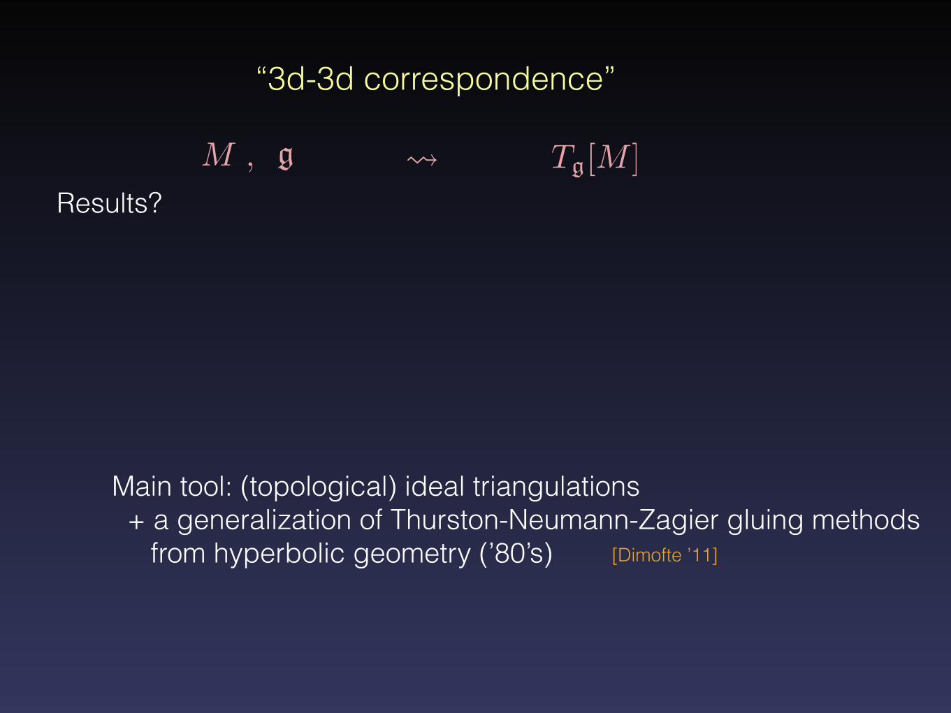
“3d-3d correspondence”

“3d-3d correspondence”
M , g Tg[M ]3-manifold A,D,E 3d (N=2) SUSY field theory
[Dimofte-Gukov-Hollands ’10]first hints:

“3d-3d correspondence”
M , g Tg[M ]3-manifold A,D,E 3d (N=2) SUSY field theory
depending only on topology of M!
[Dimofte-Gukov-Hollands ’10]first hints:

“3d-3d correspondence”
M , g Tg[M ]3-manifold A,D,E 3d (N=2) SUSY field theory
depending only on topology of M!
is a top-level top’l inv’t of
[Dimofte-Gukov-Hollands ’10]
Tg[M ] M
- its observables (quantities one can compute) all correspond to classical, quantum, or categorical topological invariants, some old, but many new.
first hints:
e.g.: hyperbolic volumeVol(M)
Mflat(M,GC)space of flat conn’sGC
[Mostow ’73]

“3d-3d correspondence”
M , g Tg[M ]3-manifold A,D,E 3d (N=2) SUSY field theory
depending only on topology of M!
is a top-level top’l inv’t of
[Dimofte-Gukov-Hollands ’10]
Tg[M ] M
- its observables (quantities one can compute) all correspond to classical, quantum, or categorical topological invariants, some old, but many new.
first hints:
e.g.: hyperbolic volumeVol(M)
Mflat(M,GC)
ZGCCS(M)
space of flat conn’sGCcomplex Chern-Simons part’n f’n
[Mostow ’73]
[Witten ’89, Reshetikhin-Turaev ’91]cf. Jones poly, WRT

“3d-3d correspondence”
M , g Tg[M ]3-manifold A,D,E 3d (N=2) SUSY field theory
depending only on topology of M!
is a top-level top’l inv’t of
[Dimofte-Gukov-Hollands ’10]
Tg[M ] M
- its observables (quantities one can compute) all correspond to classical, quantum, or categorical topological invariants, some old, but many new.
first hints:
e.g.: hyperbolic volumeVol(M)
Mflat(M,GC)
ZGCCS(M)
space of flat conn’sGCcomplex Chern-Simons part’n f’n
[Mostow ’73]
[Witten ’89, Reshetikhin-Turaev ’91]cf. Jones poly, WRTcategorification

“3d-3d correspondence”
M , g Tg[M ] [Dimofte-Gukov-Hollands ’10]first hints:
e.g.: hyperbolic volumeVol(M)
Mflat(M,GC)
ZGCCS(M)
space of flat conn’sGCcomplex Chern-Simons part’n f’n
[Mostow ’73]
[Witten ’89, Reshetikhin-Turaev ’91]cf. Jones poly, WRTcategorification
More than just theory!

“3d-3d correspondence”
M , g Tg[M ] [Dimofte-Gukov-Hollands ’10]first hints:
More than just theory!
“Most” , : explicit construction of g = sl2M Tg[M ][Dimofte-Gaiotto-Gukov ’11] [Cecotti-Cordova-Vafa ’11] [Dimofte-Gaiotto-v.d.Veen ’13]
g = sln : [Dimofte-Gabella-Goncharov ’13]

“3d-3d correspondence”
M , g Tg[M ] [Dimofte-Gukov-Hollands ’10]first hints:
More than just theory!
“Most” , : explicit construction of g = sl2M Tg[M ]
g = sln : [Dimofte-Gabella-Goncharov ’13]
Main tool: (topological) ideal triangulations + a generalization of Thurston-Neumann-Zagier gluing methods from hyperbolic geometry (’80’s) [Dimofte ’11]
[Dimofte-Gaiotto-Gukov ’11] [Cecotti-Cordova-Vafa ’11] [Dimofte-Gaiotto-v.d.Veen ’13]
“3d-3d correspondence”
M , g Tg[M ]
Main tool: (topological) ideal triangulations + a generalization of Thurston-Neumann-Zagier gluing methods from hyperbolic geometry (’80’s) [Dimofte ’11]
Results?

“3d-3d correspondence”
M , g Tg[M ]
Main tool: (topological) ideal triangulations + a generalization of Thurston-Neumann-Zagier gluing methods from hyperbolic geometry (’80’s) [Dimofte ’11]
Math:Results?
New “quantum” topological invariants,
ZGCCS(M)
for all CS levels k 2 Z [Dimofte-Gaiotto-Gukov ’11] [Dimofte ’14]
a comb’r definition of the Chern-Simons part’n functionGC

“3d-3d correspondence”
M , g Tg[M ]
Math:Results?
New “quantum” topological invariants,a comb’r definition of the Chern-Simons part’n functionGC
ZGCCS(M)
for all CS levels k 2 Z [Dimofte-Gaiotto-Gukov ’11] [Dimofte ’14]
- analyzing asymptotics of (easy!)ZGCCS(M)
simple, conjectured (tested) formula for GC-twisted Reidemeister-Ray-Singer torsion of M
[Dimofte-Garoufalidis ’12]

“3d-3d correspondence”
M , g Tg[M ]
Math:Results?
New “quantum” topological invariants,
ZGCCS(M)
for all CS levels k 2 Z [Dimofte-Gaiotto-Gukov ’11] [Dimofte ’14]
- analyzing asymptotics of (easy!)ZGCCS(M)
simple, conjectured (tested) formula for GC-twisted Reidemeister-Ray-Singer torsion of M
predictions for asymptotics of colored Jones poly’s(hard!; play a role in Volume Conjecture)[Kashaev ’97, Murakami-Murakami ’99, Gukov ‘03]
a comb’r definition of the Chern-Simons part’n functionGC
[Dimofte-Garoufalidis ’12]
[Dimofte-Garoufalidis ’15][Dimofte-Gukov-Lenells-Zagier ’08]

“3d-3d correspondence”
M , g Tg[M ]
Math:Results?
ZGCCS(M)
- analyzing asymptotics of (easy!)ZGCCS(M)
a comb’r definition of the Chern-Simons part’n functionGC
Hopefully: a combinatorial definition for 3-manifold homology!
GCin progress w/ Gaiotto-Moore
(Analogous to Khovanov homology for )G
simple, conjectured (tested) formula for GC-twisted Reidemeister-Ray-Singer torsion of M
[Dimofte-Garoufalidis ’12]
predictions for asymptotics of colored Jones poly’s(hard!; play a role in Volume Conjecture)[Kashaev ’97, Murakami-Murakami ’99, Gukov ‘03] [Dimofte-Garoufalidis ’15]
[Dimofte-Gukov-Lenells-Zagier ’08]

“3d-3d correspondence”
M , g Tg[M ]
Physics:Results?
Intuition!Properties of 3d N=2 theories are governed by the geometry of 3-manifolds!

“3d-3d correspondence”
M , g Tg[M ]
Physics:Results?
- geometric description of (IR) dualities within a large class of 3d N=2 SUSY gauge theories
(from different ways to cut/glue the same )M
Intuition!Properties of 3d N=2 theories are governed by the geometry of 3-manifolds!

“3d-3d correspondence”
M , g Tg[M ]
Physics:Results?
- geometric description of (IR) dualities within a large class of 3d N=2 SUSY gauge theories
(from different ways to cut/glue the same )M
Intuition!Properties of 3d N=2 theories are governed by the geometry of 3-manifolds!
- systematic construction of superconformal interfacesTg[M ]
4d N=2 T 4d N=2 T’
[Dimofte-Gaiotto-v.d.Veen ’13]

“3d-3d correspondence”
M , g Tg[M ]
Physics:Results?
- geometric description of (IR) dualities within a large class of 3d N=2 SUSY gauge theories
(from different ways to cut/glue the same )M
Intuition!Properties of 3d N=2 theories are governed by the geometry of 3-manifolds!
- systematic construction of superconformal interfacesTg[M ]
4d N=2 T 4d N=2 T’gYM g0YM ⇠ 1/gYMS-duality:
[Dimofte-Gaiotto-v.d.Veen ’13]

Remainder of the talk:
Tg[M ]
4d N=2 T 4d N=2 T’gYM g0YM ⇠ 1/gYMS-duality:
[Dimofte-Gaiotto-v.d.Veen ’13]

Remainder of the talk:- a few more details on the correspondence, and observables of Tg[M ]

Remainder of the talk:- a few more details on the correspondence, and observables of Tg[M ]
- tetrahedra, formulas, and examples

Remainder of the talk:- a few more details on the correspondence, and observables of Tg[M ]
- tetrahedra, formulas, and examples
- first look at homological/categorical invariants

The correspondence
Starting point: 6d (2,0) SCFT“theory ”X
[Strominger, Witten ’90’s]super-conformal-field-theory

The correspondence
Starting point: 6d (2,0) SCFT“theory ”X
[Strominger, Witten ’90’s]
(world-volume theory of M5 branes)
super-conformal-field-theory

The correspondence
Starting point: 6d (2,0) SCFT“theory ”X
[Strominger, Witten ’90’s]
(world-volume theory of M5 branes)
labelled by an ADE symmetry algebra g
super-conformal-field-theory

The correspondence
Starting point: 6d (2,0) SCFT“theory ”X
[Strominger, Witten ’90’s]
(world-volume theory of M5 branes)
X on (topological twist on M)M ⇥ R3
effective theory on
labelled by an ADE symmetry algebra
Tg[M ]
g
R3
g
super-conformal-field-theory

The correspondence
Starting point: 6d (2,0) SCFT“theory ”X
[Strominger, Witten ’90’s]
(world-volume theory of M5 branes)
X on (topological twist on M)M ⇥ R3
effective theory on
labelled by an ADE symmetry algebra
Tg[M ]
g
R3
g
How to describe ?Tg[M ]
super-conformal-field-theory

The correspondence
Starting point: 6d (2,0) SCFT“theory ”X
[Strominger, Witten ’90’s]
(world-volume theory of M5 branes)
X on (topological twist on M)M ⇥ R3
effective theory on
labelled by an ADE symmetry algebra
Tg[M ]
g
R3
g
How to describe ?Tg[M ]
- direct, first-principles is hard: X has no Lagrangian
super-conformal-field-theory

The correspondence
Starting point: 6d (2,0) SCFT“theory ”X
[Strominger, Witten ’90’s]
(world-volume theory of M5 branes)
X on (topological twist on M)M ⇥ R3
effective theory on
labelled by an ADE symmetry algebra
Tg[M ]
g
R3
g
How to describe ?Tg[M ]
- direct, first-principles is hard: X has no Lagrangian- nevertheless, can infer many properties of + its compact’nsTg[M ]
super-conformal-field-theory

The correspondence
How to describe ?Tg[M ]
- direct, first-principles is hard: X has no Lagrangian- nevertheless, can infer many properties of + its compact’nsTg[M ]
{vacua of on }
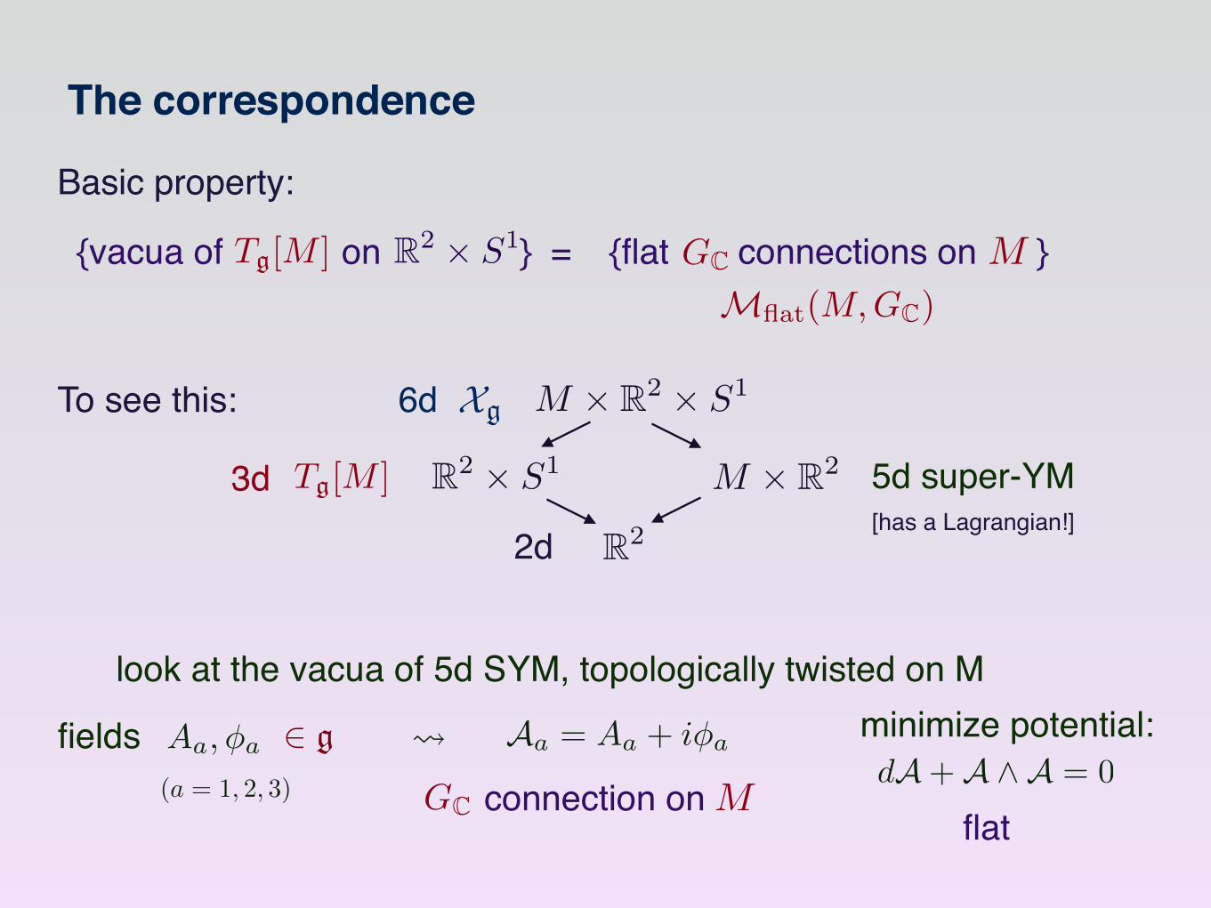
Basic property:
Tg[M ] R2 ⇥ S1 = {flat connections on }GC M
Mflat(M,GC)
To see this: 6d M ⇥ R2 ⇥ S1
R2
R2 ⇥ S1
Xg
Tg[M ]3d
2d

The correspondence
How to describe ?Tg[M ]
- direct, first-principles is hard: X has no Lagrangian- nevertheless, can infer many properties of + its compact’nsTg[M ]
{vacua of on }
Basic property:
Tg[M ] R2 ⇥ S1 = {flat connections on }GC M
Mflat(M,GC)
To see this: 6d M ⇥ R2 ⇥ S1
M ⇥ R2
R2
R2 ⇥ S1
Xg
Tg[M ]3d
2d
5d super-YM[has a Lagrangian!]

The correspondence
{vacua of on }
Basic property:
Tg[M ] R2 ⇥ S1 = {flat connections on }GC M
Mflat(M,GC)
To see this: 6d M ⇥ R2 ⇥ S1
M ⇥ R2
R2
R2 ⇥ S1
Xg
Tg[M ]3d
2d
5d super-YM
look at the vacua of 5d SYM, topologically twisted on M
[has a Lagrangian!]

The correspondence
{vacua of on }
Basic property:
Tg[M ] R2 ⇥ S1 = {flat connections on }GC M
Mflat(M,GC)
To see this: 6d M ⇥ R2 ⇥ S1
M ⇥ R2
R2
R2 ⇥ S1
Xg
Tg[M ]3d
2d
5d super-YM
look at the vacua of 5d SYM, topologically twisted on M
Aa,�a
(a = 1, 2, 3)
[has a Lagrangian!]
fields 2 g

The correspondence
{vacua of on }
Basic property:
Tg[M ] R2 ⇥ S1 = {flat connections on }GC M
Mflat(M,GC)
To see this: 6d M ⇥ R2 ⇥ S1
M ⇥ R2
R2
R2 ⇥ S1
Xg
Tg[M ]3d
2d
5d super-YM
look at the vacua of 5d SYM, topologically twisted on M
Aa,�a Aa = Aa + i�a
(a = 1, 2, 3)
[has a Lagrangian!]
fieldsGC connection on M
2 g
The correspondence
{vacua of on }
Basic property:
Tg[M ] R2 ⇥ S1 = {flat connections on }GC M
Mflat(M,GC)
To see this: 6d M ⇥ R2 ⇥ S1
M ⇥ R2
R2
R2 ⇥ S1
Xg
Tg[M ]3d
2d
5d super-YM
look at the vacua of 5d SYM, topologically twisted on M
Aa,�a Aa = Aa + i�a
(a = 1, 2, 3)
[has a Lagrangian!]
fieldsGC connection on M
2 g minimize potential:dA+A ^A = 0
flat

The correspondence
{vacua on }R2 ⇥ S1 = {flat connections}GC
MTg[M ]
Mflat(M,GC)[Dimofte-Gukov-Hollands ’10]
look at the vacua of 5d SYM, topologically twisted on M
Aa,�a Aa = Aa + i�a
(a = 1, 2, 3)
fieldsGC connection on M
2 g minimize potential:dA+A ^A = 0
flat

The correspondence
{vacua on }R2 ⇥ S1 = {flat connections}GC
MTg[M ]
Mflat(M,GC)[Dimofte-Gukov-Hollands ’10]
quantize!
look at the vacua of 5d SYM, topologically twisted on M
Aa,�a Aa = Aa + i�a
(a = 1, 2, 3)
fieldsGC connection on M
2 g minimize potential:dA+A ^A = 0
flat

The correspondence
{vacua on }R2 ⇥ S1 = {flat connections}GC
MTg[M ]
Mflat(M,GC)[Dimofte-Gukov-Hollands ’10]
quantize!
Chern-Simons theory on MGC
ZCS [M ] =
ZDADA e
k+i�8⇡i ICS(A)+
k�i�8⇡i ICS(A)
ICS(A) :=
Z
MTr
⇣A ^ dA+
2
3A ^A ^A
⌘
[Witten ’91]
A gC-valued 1-form:

The correspondence
{vacua on }R2 ⇥ S1 = {flat connections}GC
MTg[M ]
Mflat(M,GC)[Dimofte-Gukov-Hollands ’10]
quantize!
Chern-Simons theory on MGC
ZCS [M ] =
ZDADA e
k+i�8⇡i ICS(A)+
k�i�8⇡i ICS(A)
ICS(A) :=
Z
MTr
⇣A ^ dA+
2
3A ^A ^A
⌘
[Witten ’91]
k 2 Z � 2 R (or C)
A gC-valued 1-form:

The correspondence
{vacua on }R2 ⇥ S1 = {flat connections}GC
MTg[M ]
Mflat(M,GC)[Dimofte-Gukov-Hollands ’10]
quantize!
Chern-Simons theory on MGC
ZCS [M ] =
ZDADA e
k+i�8⇡i ICS(A)+
k�i�8⇡i ICS(A)
ICS(A) :=
Z
MTr
⇣A ^ dA+
2
3A ^A ^A
⌘
[Witten ’91]
k 2 Z � 2 R (or C)
A gC-valued 1-form:
- classical sol’ns are flat connectionsGC

The correspondence
{vacua on }R2 ⇥ S1 = {flat connections}GC
MTg[M ]
Mflat(M,GC)[Dimofte-Gukov-Hollands ’10]
quantize!
Chern-Simons theory on MGC
ZCS [M ] =
ZDADA e
k+i�8⇡i ICS(A)+
k�i�8⇡i ICS(A)
ICS(A) :=
Z
MTr
⇣A ^ dA+
2
3A ^A ^A
⌘
[Witten ’91]
k 2 Z � 2 R (or C)
- classical sol’ns are flat connections
A gC-valued 1-form:
GC
- cf. compact CS thy: on knot complements, get Jones polysG[Witten ’89]
(combinatorial definition) [Reshetikhin-Turaev ’90, etc.]
- combinatorial def’n missing for until recently!GC

The correspondence
{vacua on }R2 ⇥ S1 = {flat connections}GC
MTg[M ]
Mflat(M,GC)[Dimofte-Gukov-Hollands ’10]
ZCS [M ] =
ZDADA e
k+i�8⇡i ICS(A)+
k�i�8⇡i ICS(A)
ICS(A) :=
Z
MTr
⇣A ^ dA+
2
3A ^A ^A
⌘
[Witten ’91]
k 2 Z � 2 R (or C)
- classical sol’ns are flat connectionsGC
- cf. compact CS thy: on knot complements, get Jones polysG[Witten ’89]
(combinatorial definition) [Reshetikhin-Turaev ’90, etc.]
- combinatorial def’n missing for until recently!GC
Z(k,�)CS [M ]

The correspondence
{vacua on }R2 ⇥ S1 = {flat connections}GC
MTg[M ]
Mflat(M,GC)[Dimofte-Gukov-Hollands ’10]
ZCS [M ] =
ZDADA e
k+i�8⇡i ICS(A)+
k�i�8⇡i ICS(A)
ICS(A) :=
Z
MTr
⇣A ^ dA+
2
3A ^A ^A
⌘
[Witten ’91]
k 2 Z � 2 R (or C)
- classical sol’ns are flat connectionsGC
- cf. compact CS thy: on knot complements, get Jones polysG[Witten ’89]
(combinatorial definition) [Reshetikhin-Turaev ’90, etc.]
- combinatorial def’n missing for until recently!GC
Z(k,�)CS [M ]=ZTg[M ][L(k, 1)�]
part’n function onellipsoidally-deformed lens space

The correspondence
{vacua on }R2 ⇥ S1 = {flat connections}GC
MTg[M ]
Mflat(M,GC)[Dimofte-Gukov-Hollands ’10]
Z(k,�)CS [M ]=ZTg[M ][L(k, 1)�]
part’n function onellipsoidally-deformed lens space
L(k, 1)� = S3�/Zk
' {b2|z|2 + b�2|w|2 = 1} 2 C2.(z, w) ⇠ (e
2⇡ik z, e
2⇡ik w)
b2 =k � i�
k + i�

The correspondence
{vacua on }R2 ⇥ S1 = {flat connections}GC
MTg[M ]
Mflat(M,GC)[Dimofte-Gukov-Hollands ’10]
Z(k,�)CS [M ]=ZTg[M ][L(k, 1)�]
part’n function onellipsoidally-deformed lens space
L(k, 1)� = S3�/Zk
' {b2|z|2 + b�2|w|2 = 1} 2 C2.(z, w) ⇠ (e
2⇡ik z, e
2⇡ik w)b2 =
k � i�
k + i�
k=1 :[Terashima-Yamazaki ’11]![Dimofte-Gaiotto-Gukov ’11][Cordova-Jafferis ’13] — physical proof

The correspondence
{vacua on }R2 ⇥ S1 = {flat connections}GC
MTg[M ]
Mflat(M,GC)[Dimofte-Gukov-Hollands ’10]
Z(k,�)CS [M ]=ZTg[M ][L(k, 1)�]
part’n function onellipsoidally-deformed lens space
L(k, 1)� = S3�/Zk
' {b2|z|2 + b�2|w|2 = 1} 2 C2.(z, w) ⇠ (e
2⇡ik z, e
2⇡ik w)b2 =
k � i�
k + i�
k=0 :
k=1 :
[Dimofte-Gaiotto-Gukov (2) ’11]
[Terashima-Yamazaki ’11]![Dimofte-Gaiotto-Gukov ’11][Cordova-Jafferis ’13]
[Lee-Yamazaki ’13]
— physical proof
— physical proof

The correspondence
{vacua on }R2 ⇥ S1 = {flat connections}GC
MTg[M ]
Mflat(M,GC)[Dimofte-Gukov-Hollands ’10]
Z(k,�)CS [M ]=ZTg[M ][L(k, 1)�]
part’n function onellipsoidally-deformed lens space
L(k, 1)� = S3�/Zk
' {b2|z|2 + b�2|w|2 = 1} 2 C2.(z, w) ⇠ (e
2⇡ik z, e
2⇡ik w)
k=0 :
b2 =k � i�
k + i�
k=1 :
general k:
[Dimofte-Gaiotto-Gukov (2) ’11]
[Terashima-Yamazaki ’11]![Dimofte-Gaiotto-Gukov ’11][Cordova-Jafferis ’13]
[Dimofte ’14]
[Lee-Yamazaki ’13]
— physical proof
— physical proof

The correspondence
{vacua on }R2 ⇥ S1 = {flat connections}GC
MTg[M ]
Mflat(M,GC)[Dimofte-Gukov-Hollands ’10]
Z(k,�)CS [M ]=ZTg[M ][L(k, 1)�]
k=0 : [Dimofte-Gaiotto-Gukov (2) ’11]
k=1 : [Terashima-Yamazaki ’11]![Dimofte-Gaiotto-Gukov ’11][Cordova-Jafferis ’13]
general k: [Dimofte ’14]
to tie this all together:
Zk,�CS [M ] =
X
flat ↵
Bk+i�↵ [M ]Bk+i�
↵ [M ]
[Lee-Yamazaki ’13]
— physical proof
— physical proof

The correspondence
{vacua on }R2 ⇥ S1 = {flat connections}GC
MTg[M ]
Mflat(M,GC)[Dimofte-Gukov-Hollands ’10]
Z(k,�)CS [M ]=ZTg[M ][L(k, 1)�]
k=0 :
k=1 :
general k:
to tie this all together:
Zk,�CS [M ] =
X
flat ↵
Bk+i�↵ [M ]Bk+i�
↵ [M ]
[Beem-Dimofte-Pasquetti ‘12]
ZTg[M ][L(k, 1)�] =X
vacua ↵
Bk+i�↵ [M ]Bk+i�
↵ [M ]
L(k, 1) ' (D2 ⇥ S1) ['2SL(2,Z) (D2 ⇥ S1)
[Dimofte-Gaiotto-Gukov (2) ’11]
[Terashima-Yamazaki ’11]![Dimofte-Gaiotto-Gukov ’11][Cordova-Jafferis ’13]
[Dimofte ’14]
[Lee-Yamazaki ’13]
— physical proof
— physical proof

The correspondence
{vacua on }R2 ⇥ S1 = {flat connections}GC
MTg[M ]
Mflat(M,GC)
Z(k,�)CS [M ]=ZTg[M ][L(k, 1)�]
to tie this all together:
Zk,�CS [M ] =
X
flat ↵
Bk+i�↵ [M ]Bk+i�
↵ [M ]
[Beem-Dimofte-Pasquetti ‘12]
ZTg[M ][L(k, 1)�] =X
vacua ↵
Bk+i�↵ [M ]Bk+i�
↵ [M ]
L(k, 1) ' (D2 ⇥ S1) ['2SL(2,Z) (D2 ⇥ S1)
So: quantum invariants of 3-manifolds! can be understood via 3d SUSY theories on lens spaces!

The correspondence
{vacua on }R2 ⇥ S1 = {flat connections}GC
MTg[M ]
Mflat(M,GC)
Z(k,�)CS [M ]=ZTg[M ][L(k, 1)�]
So: quantum invariants of 3-manifolds! can be understood via 3d SUSY theories on lens spaces!
One more step: categorify

The correspondence
{vacua on }R2 ⇥ S1 = {flat connections}GC
MTg[M ]
Mflat(M,GC)
Z(k,�)CS [M ]=ZTg[M ][L(k, 1)�]
So: quantum invariants of 3-manifolds! can be understood via 3d SUSY theories on lens spaces!
One more step: categorify
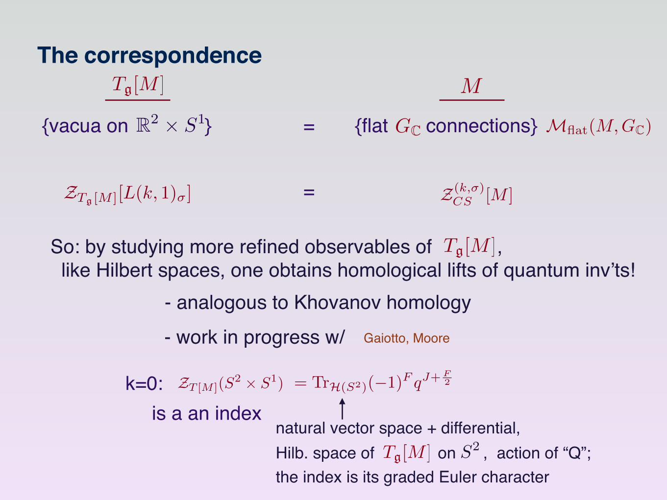
ZT [M ](S2 ⇥ S1)k=0:
is a an index= TrH(S2)(�1)F qJ+
F2

The correspondence
{vacua on }R2 ⇥ S1 = {flat connections}GC
MTg[M ]
Mflat(M,GC)
Z(k,�)CS [M ]=ZTg[M ][L(k, 1)�]
So: quantum invariants of 3-manifolds! can be understood via 3d SUSY theories on lens spaces!
One more step: categorify
ZT [M ](S2 ⇥ S1)k=0:
is a an index= TrH(S2)(�1)F qJ+
F2
natural vector space + differential,Tg[M ] S2Hilb. space of on , action of “Q”;

The correspondence
{vacua on }R2 ⇥ S1 = {flat connections}GC
MTg[M ]
Mflat(M,GC)
Z(k,�)CS [M ]=ZTg[M ][L(k, 1)�]
So: quantum invariants of 3-manifolds! can be understood via 3d SUSY theories on lens spaces!
One more step: categorify
ZT [M ](S2 ⇥ S1)k=0:
is a an index= TrH(S2)(�1)F qJ+
F2
natural vector space + differential,Hilb. space of on , action of “Q”;Tg[M ] S2
the index is its graded Euler character

The correspondence
{vacua on }R2 ⇥ S1 = {flat connections}GC
MTg[M ]
Mflat(M,GC)
Z(k,�)CS [M ]=ZTg[M ][L(k, 1)�]
So: by studying more refined observables of ,! like Hilbert spaces, one obtains homological lifts of quantum inv’ts!
One more step: categorify
ZT [M ](S2 ⇥ S1)k=0:
is a an index= TrH(S2)(�1)F qJ+
F2
natural vector space + differential,Hilb. space of on , action of “Q”;Tg[M ] S2
the index is its graded Euler character
Tg[M ]
- analogous to Khovanov homology
The correspondence
{vacua on }R2 ⇥ S1 = {flat connections}GC
MTg[M ]
Mflat(M,GC)
Z(k,�)CS [M ]=ZTg[M ][L(k, 1)�]
ZT [M ](S2 ⇥ S1)k=0:
is a an index= TrH(S2)(�1)F qJ+
F2
natural vector space + differential,Hilb. space of on , action of “Q”;Tg[M ] S2
the index is its graded Euler character
So: by studying more refined observables of ,! like Hilbert spaces, one obtains homological lifts of quantum inv’ts!
Tg[M ]
- analogous to Khovanov homology- work in progress w/ Gaiotto, Moore

The correspondence
{vacua on }R2 ⇥ S1 = {flat connections}GC
MTg[M ]
Mflat(M,GC)
Z(k,�)CS [M ]=ZTg[M ][L(k, 1)�]
- analogous to Khovanov homology- work in progress w/ Gaiotto, Moore
So: by studying more refined observables of ,! like Hilbert spaces, one obtains homological lifts of quantum inv’ts!
Tg[M ]
This was the “pedestrian” version!

The correspondence
{vacua on }R2 ⇥ S1 = {flat connections}GC
MTg[M ]
Mflat(M,GC)
Z(k,�)CS [M ]=ZTg[M ][L(k, 1)�]
- analogous to Khovanov homology- work in progress w/ Gaiotto, Moore
This was the “pedestrian” version!
So: by studying more refined observables of ,! like Hilbert spaces, one obtains homological lifts of quantum inv’ts!
Tg[M ]
Full picture: study with boundaryM

The correspondence
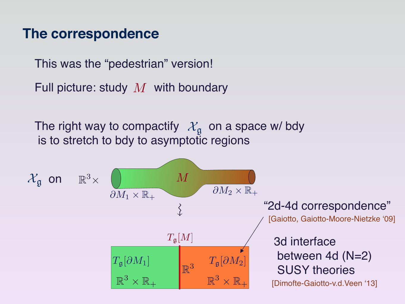
This was the “pedestrian” version!
Full picture: study with boundaryM
The right way to compactify on a space w/ bdy! is to stretch to bdy to asymptotic regions
Xg
Xg on R3⇥ M
@M1 ⇥ R+@M2 ⇥ R+

The correspondence
This was the “pedestrian” version!
Full picture: study with boundaryM
The right way to compactify on a space w/ bdy! is to stretch to bdy to asymptotic regions
Xg
Xg on R3⇥
M
Tg[M ]
R3
R3 ⇥ R+R3 ⇥ R+
Tg[@M1] Tg[@M2]
@M1 ⇥ R+@M2 ⇥ R+
3d interface! between 4d (N=2)! SUSY theories[Dimofte-Gaiotto-v.d.Veen ‘13]
The correspondence
This was the “pedestrian” version!
Full picture: study with boundaryM
The right way to compactify on a space w/ bdy! is to stretch to bdy to asymptotic regions
Xg
Xg on R3⇥
M
Tg[M ]
R3
R3 ⇥ R+R3 ⇥ R+
Tg[@M1] Tg[@M2]
@M1 ⇥ R+@M2 ⇥ R+
“2d-4d correspondence”[Gaiotto, Gaiotto-Moore-Nietzke ‘09]
3d interface! between 4d (N=2)! SUSY theories[Dimofte-Gaiotto-v.d.Veen ‘13]

The correspondence is functorial:
Xg on R3⇥
M
Tg[M ]
R3
R3 ⇥ R+R3 ⇥ R+
Tg[@M1] Tg[@M2]
@M1 ⇥ R+@M2 ⇥ R+
“2d-4d correspondence”[Gaiotto, Gaiotto-Moore-Nietzke ‘09]
3d interface! between 4d (N=2)! SUSY theories[Dimofte-Gaiotto-v.d.Veen ‘13]

The correspondence is functorial:
Tg : Cobordism category of 2-manifolds
objects: 2-manifoldsmorphisms: 3-cobordisms
Cat. of 4d N=2 SUSY thy’sobjects: 4d theoriesmorphisms: 3d interfaces
Xg on R3⇥
M
Tg[M ]
R3
R3 ⇥ R+R3 ⇥ R+
Tg[@M1] Tg[@M2]
@M1 ⇥ R+@M2 ⇥ R+
“2d-4d correspondence”[Gaiotto, Gaiotto-Moore-Nietzke ‘09]
3d interface! between 4d (N=2)! SUSY theories[Dimofte-Gaiotto-v.d.Veen ‘13]

The correspondence is functorial:
Tg : Cobordism category of 2-manifolds
objects: 2-manifoldsmorphisms: 3-cobordisms
Can extend further,
2-morphisms: 4-cobordisms
Cat. of 4d N=2 SUSY thy’sobjects: 4d theoriesmorphisms: 3d interfaces

The correspondence is functorial:
Tg : Cobordism category of 2-manifolds
objects: 2-manifoldsmorphisms: 3-cobordisms
Can extend further,
2-morphisms: 4-cobordisms 2-morphisms: 2d interfaces
cf. [Gadde-Gukov-Putrov ’13]“4d-2d correspondence”
Cat. of 4d N=2 SUSY thy’sobjects: 4d theoriesmorphisms: 3d interfaces

The correspondence is effective

The correspondence is effective
For a large class of 3-manifolds, can explicitly compute Tg[M ]
give an explicit 3d Lagrangian density

The correspondence is effective
For a large class of 3-manifolds, can explicitly compute Tg[M ]
give an explicit 3d Lagrangian density
- includes all hyperbolic , with cusps and/or geodesic bdyM

The correspondence is effective
For a large class of 3-manifolds, can explicitly compute Tg[M ]
give an explicit 3d Lagrangian density
- includes all hyperbolic , with cusps and/or geodesic bdyM
(most 3-manifolds are hyperbolic= admit a metric of constant neg. curvature)
(given appropriate boundary conditions, the metric is unique)[Mostow ’76,…]
- method of computation: cut M into (topological) ideal tetrahedra
truncated vertices

The correspondence is effective
For a large class of 3-manifolds, can explicitly compute Tg[M ]
give an explicit 3d Lagrangian density
- includes all hyperbolic , with cusps and/or geodesic bdyM
(most 3-manifolds are hyperbolic= admit a metric of constant neg. curvature)
(given appropriate boundary conditions, the metric is unique)[Mostow ’76,…]
- method of computation: cut M into (topological) ideal tetrahedra
truncated verticesTg[M ] =
✓ NOi=1
Tg[�i]
◆�⇠M =
N[
i=1
�i

The correspondence is effective
Tg[M ] =
✓ NOi=1
Tg[�i]
◆�⇠M =
N[
i=1
�i
Remainder of the talk: g = sl2 GC = SL(2,C) (or PSL(2,C)= SL(2,C)/{±1})

The correspondence is effective
Tg[M ] =
✓ NOi=1
Tg[�i]
◆�⇠M =
N[
i=1
�i
Remainder of the talk: g = sl2 GC = SL(2,C) (or PSL(2,C)
- for simplicity, and some added intuition g = sln[Dimofte-Gabella-Goncharov ’13]
= SL(2,C)/{±1})

The correspondence is effective
Tg[M ] =
✓ NOi=1
Tg[�i]
◆�⇠M =
N[
i=1
�i
Remainder of the talk: g = sl2 GC = SL(2,C) (or PSL(2,C)
- for simplicity, and some added intuition g = sln[Dimofte-Gabella-Goncharov ’13]
- flat connections are (roughly) hyperbolic metricsPSL(2,C)
= SL(2,C)/{±1})
So: quantizes, categorifies, etc. classical hyperbolic geometry!Tg[M ]

The correspondence is effectiveSingle (ideal, hyperbolic) tetrahedron:
0
1
1
z
@H3 ' C [ {1}

The correspondence is effectiveSingle (ideal, hyperbolic) tetrahedron:
0
1
1
z
@H3
- vertices at on the bdy of H3
- faces are geodesic surfaces
' C [ {1}

The correspondence is effectiveSingle (ideal, hyperbolic) tetrahedron:
- vertices at on the bdy of H3
- faces are geodesic surfaces0
1
1
z
@H3 ' C [ {1}
- the hyperbolic structure is encoded! in 6 complexified dihedral angles
zz0
z00
z
z0
z00
z = e(torsion)+i(angle)

The correspondence is effectiveSingle (ideal, hyperbolic) tetrahedron:
- vertices at on the bdy of H3
- faces are geodesic surfaces0
1
1
z
@H3 ' C [ {1}
- the hyperbolic structure is encoded! in 6 complexified dihedral angles
zz0
z00
zz0z00 = �1
z00 + z�1 � 1 = 0
z
z0
z00
z = e(torsion)+i(angle)
equal on opposite edges,!and satisfy [W. Thurston, late ’70’s]

The correspondence is effectiveSingle (ideal, hyperbolic) tetrahedron:
- vertices at on the bdy of H3
- faces are geodesic surfaces
0
1
1
z
@H3 ' C [ {1}
- the hyperbolic structure is encoded! in 6 complexified dihedral angles
zz0
z00
zz0z00 = �1
z00 + z�1 � 1 = 0
z
z0
z00z = e(torsion)+i(angle)
equal on opposite edges,!and satisfy [W. Thurston, late ’70’s]
Flat connections: Mflat(@�, GC) ⇡ C⇤ ⇥ C⇤ (z, z00) [Dimofte ’10]

The correspondence is effectiveSingle (ideal, hyperbolic) tetrahedron:
- vertices at on the bdy of H3
- faces are geodesic surfaces
0
1
1
z
@H3 ' C [ {1}
- the hyperbolic structure is encoded! in 6 complexified dihedral angles
zz0
z00
zz0z00 = �1
z00 + z�1 � 1 = 0
z
z0
z00z = e(torsion)+i(angle)
equal on opposite edges,!and satisfy [W. Thurston, late ’70’s]
Flat connections: Mflat(@�, GC) ⇡ C⇤ ⇥ C⇤ (z, z00)
Mflat(�, GC) = {z00 + z�1 � 1 = 0}
[Dimofte ’10]
⇢ ⇢

The correspondence is effectiveTetrahedron theory:
0
1
1
z
@H3
zz0
z00
zz0z00 = �1
z00 + z�1 � 1 = 0
z
z0
z00
Flat connections: Mflat(@�, GC) ⇡ C⇤ ⇥ C⇤ (z, z00)
Mflat(�, GC) = {z00 + z�1 � 1 = 0}
[Dimofte ’10]
⇢ ⇢
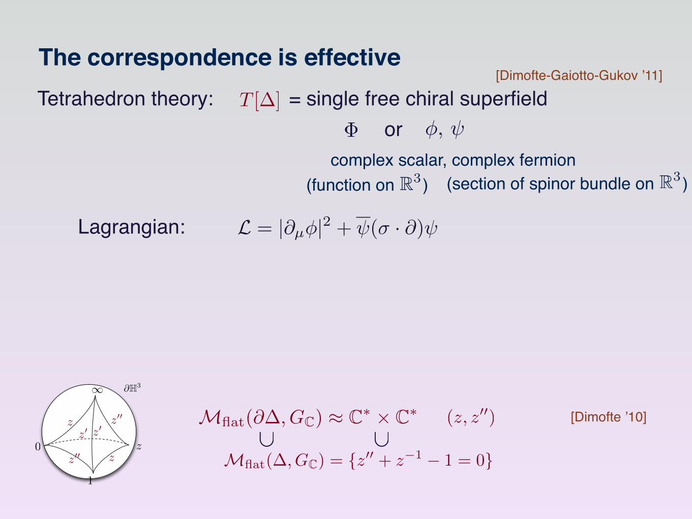
= single free chiral superfieldT [�]
[Dimofte-Gaiotto-Gukov ’11]

The correspondence is effectiveTetrahedron theory:
zz0z00 = �1
z00 + z�1 � 1 = 0
0
1
1
z
@H3
zz0
z00
z
z0
z00
Flat connections: Mflat(@�, GC) ⇡ C⇤ ⇥ C⇤ (z, z00)
Mflat(�, GC) = {z00 + z�1 � 1 = 0}
[Dimofte ’10]
⇢ ⇢
= single free chiral superfieldT [�]
complex scalar, complex fermion� �, or
(function on )R3 (section of spinor bundle on )R3
[Dimofte-Gaiotto-Gukov ’11]
The correspondence is effectiveTetrahedron theory:
Mflat(@�, GC) ⇡ C⇤ ⇥ C⇤ (z, z00)
Mflat(�, GC) = {z00 + z�1 � 1 = 0}
[Dimofte ’10]
⇢ ⇢
= single free chiral superfieldT [�]
complex scalar, complex fermion� �, or
(function on )R3 (section of spinor bundle on )R3
0
1
1
z
@H3
zz0
z00
z
z0
z00
[Dimofte-Gaiotto-Gukov ’11]
L = |@µ�|2 + (� · @) Lagrangian:

The correspondence is effectiveTetrahedron theory:
Mflat(@�, GC) ⇡ C⇤ ⇥ C⇤ (z, z00)
Mflat(�, GC) = {z00 + z�1 � 1 = 0}
[Dimofte ’10]
⇢ ⇢
= single free chiral superfieldT [�]
complex scalar, complex fermion� �, or
(function on )R3 (section of spinor bundle on )R3
0
1
1
z
@H3
zz0
z00
z
z0
z00
[Dimofte-Gaiotto-Gukov ’11]
This theory allows a supersymmetric mass term Z (equal for )�,
L = |@µ�|2 + (� · @) Lagrangian: +Z|�|2 + Z
(real)

The correspondence is effectiveTetrahedron theory:
Mflat(@�, GC) ⇡ C⇤ ⇥ C⇤ (z, z00)
Mflat(�, GC) = {z00 + z�1 � 1 = 0}
[Dimofte ’10]
⇢ ⇢
= single free chiral superfieldT [�]
complex scalar, complex fermion� �, or
(function on )R3 (section of spinor bundle on )R3
0
1
1
z
@H3
zz0
z00
z
z0
z00
[Dimofte-Gaiotto-Gukov ’11]
This theory allows a supersymmetric mass term Z (equal for )�,
L = |@µ�|2 + (� · @) Lagrangian: +Z|�|2 + Z
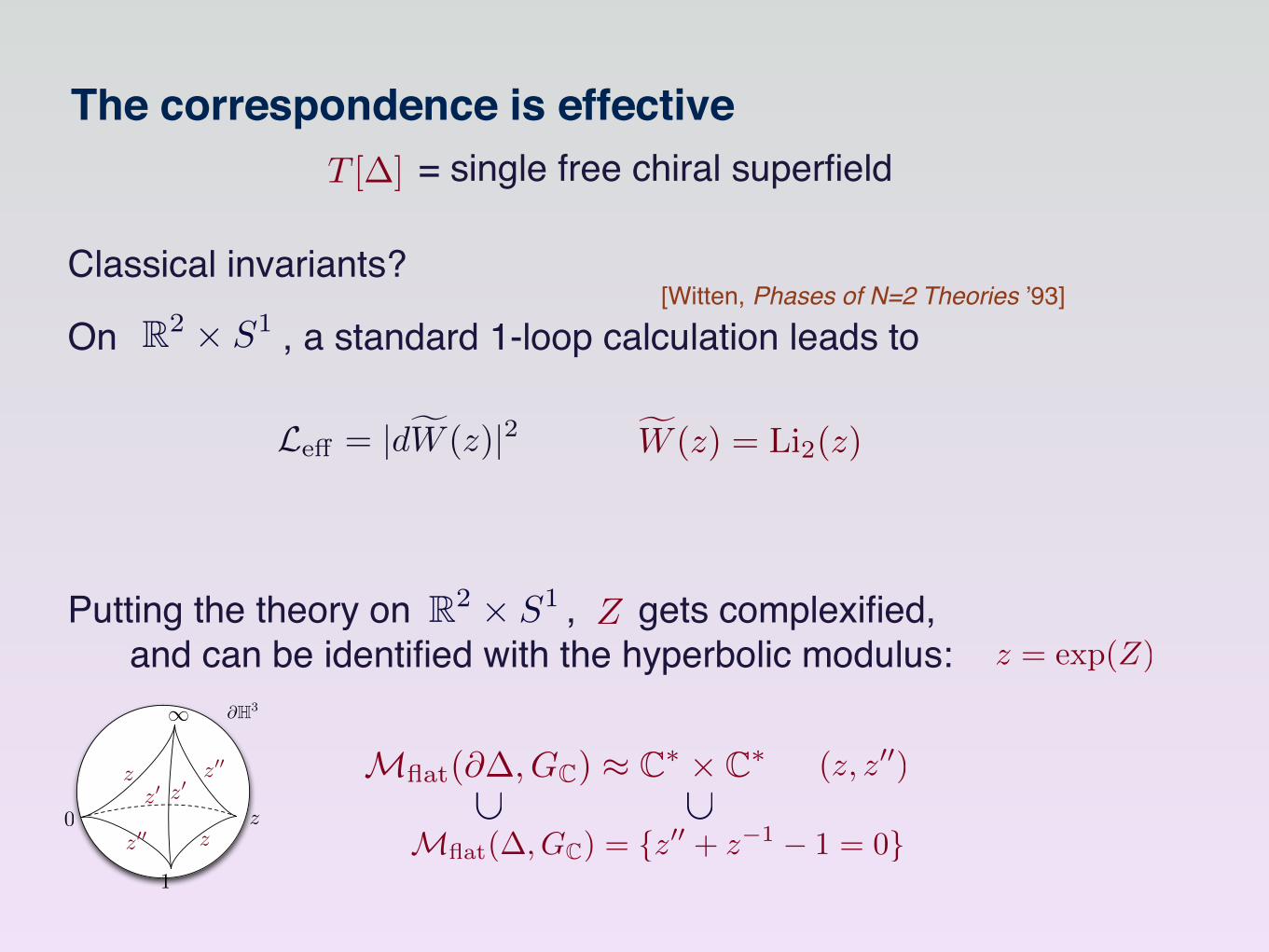
Putting the theory on , gets complexified,! and can be identified with the hyperbolic modulus:
R2 ⇥ S1
(real)
Zz = exp(Z)

The correspondence is effectiveTetrahedron theory:
Mflat(@�, GC) ⇡ C⇤ ⇥ C⇤ (z, z00)
Mflat(�, GC) = {z00 + z�1 � 1 = 0}
[Dimofte ’10]
⇢ ⇢
= single free chiral superfieldT [�]
complex scalar, complex fermion� �, or
(function on )R3 (section of spinor bundle on )R3
0
1
1
z
@H3
zz0
z00
z
z0
z00
[Dimofte-Gaiotto-Gukov ’11]
This theory allows a supersymmetric mass term Z (equal for )�,
L = |@µ�|2 + (� · @) Lagrangian: +Z|�|2 + Z
Putting the theory on , gets complexified,! and can be identified with the hyperbolic modulus:
R2 ⇥ S1
(real)
Zz = exp(Z)

The correspondence is effective
Mflat(@�, GC) ⇡ C⇤ ⇥ C⇤ (z, z00)
Mflat(�, GC) = {z00 + z�1 � 1 = 0}
⇢ ⇢
= single free chiral superfieldT [�]
0
1
1
z
@H3
zz0
z00
z
z0
z00
Putting the theory on , gets complexified,! and can be identified with the hyperbolic modulus:
R2 ⇥ S1 Zz = exp(Z)
Classical invariants?
On , a standard 1-loop calculation leads toR2 ⇥ S1
Le↵ = |dfW (z)|2 fW (z) = Li2(z)
[Witten, Phases of N=2 Theories ’93]

The correspondence is effective
Mflat(@�, GC) ⇡ C⇤ ⇥ C⇤ (z, z00)
Mflat(�, GC) = {z00 + z�1 � 1 = 0}
⇢ ⇢
= single free chiral superfieldT [�]
0
1
1
z
@H3
zz0
z00
z
z0
z00
Putting the theory on , gets complexified,! and can be identified with the hyperbolic modulus:
R2 ⇥ S1 Zz = exp(Z)
Classical invariants?
On , a standard 1-loop calculation leads toR2 ⇥ S1
Le↵ = |dfW (z)|2 fW (z) = Li2(z)
(complex) volume of !�
[Witten, Phases of N=2 Theories ’93]

The correspondence is effective
Mflat(@�, GC) ⇡ C⇤ ⇥ C⇤ (z, z00)
Mflat(�, GC) = {z00 + z�1 � 1 = 0}
⇢ ⇢
= single free chiral superfieldT [�]
0
1
1
z
@H3
zz0
z00
z
z0
z00
Classical invariants?
On , a standard 1-loop calculation leads toR2 ⇥ S1
Le↵ = |dfW (z)|2 fW (z) = Li2(z)
(complex) volume of !�
[Witten, Phases of N=2 Theories ’93]
Also, vacua of on given by T [�] R2 ⇥ S1exp
⇣zdfW (z)
dz
⌘= z00
) z00 + z�1 � 1 = 0 !

The correspondence is effective
Mflat(@�, GC) ⇡ C⇤ ⇥ C⇤ (z, z00)
Mflat(�, GC) = {z00 + z�1 � 1 = 0}
⇢ ⇢
= single free chiral superfieldT [�]
0
1
1
z
@H3
zz0
z00
z
z0
z00
Also, vacua of on given by T [�] R2 ⇥ S1exp
⇣zdfW (z)
dz
⌘= z00
) z00 + z�1 � 1 = 0 !
Turn the crank: quantum invariants

The correspondence is effective
Mflat(@�, GC) ⇡ C⇤ ⇥ C⇤ (z, z00)
Mflat(�, GC) = {z00 + z�1 � 1 = 0}
⇢ ⇢
= single free chiral superfieldT [�]
0
1
1
z
@H3
zz0
z00
z
z0
z00
Also, vacua of on given by T [�] R2 ⇥ S1exp
⇣zdfW (z)
dz
⌘= z00
) z00 + z�1 � 1 = 0 !
ZT [�][L(k, 1)�]The lens-space partition functionscan all be calculated explicitly — due to SUSY, the path integral!reduces to a finite-dimensional integral.
[Kapustin-Willett-Yaakov ’10][Hama-Hosomochi-Lee ’11]
[Kim ’09]
[Benini-Nishioka-Yamazaki ’11]
Turn the crank: quantum invariants

The correspondence is effective= single free chiral superfieldT [�]
ZT [�][L(k, 1)�]The lens-space partition functionscan all be calculated explicitly — due to SUSY, the path integral!reduces to a finite-dimensional integral.
[Kapustin-Willett-Yaakov ’10][Hama-Hosomochi-Lee ’11]
[Kim ’09]
[Benini-Nishioka-Yamazaki ’11]
Turn the crank: quantum invariants
E.g. ZT [�][S2 ⇥ S1] =
1Y
r=0
1� q1�m2 ⇣�1
1� q�m2 ⇣
q = e2⇡�
depends on , phasem 2 Z |⇣| = 1 — because has a bdy�

The correspondence is effective= single free chiral superfieldT [�]
Turn the crank: quantum invariants
E.g. ZT [�][S2 ⇥ S1] =
1Y
r=0
1� q1�m2 ⇣�1
1� q�m2 ⇣
q = e2⇡�
depends on , phasem 2 Z |⇣| = 1 — because has a bdy�
z ⇠ qm2 ⇣
z̄ ⇠ qm2 ⇣�1

The correspondence is effective= single free chiral superfieldT [�]
Turn the crank: quantum invariants
E.g. ZT [�][S2 ⇥ S1] =
1Y
r=0
1� q1�m2 ⇣�1
1� q�m2 ⇣
q = e2⇡�
depends on , phasem 2 Z |⇣| = 1 — because has a bdy�
z ⇠ qm2 ⇣
z̄ ⇠ qm2 ⇣�1
is a version of a “quantum dilogarithm”ZT [�][S2 ⇥ S1]
ZT [�][S2 ⇥ S1]
� ! 1q ! 1
⇠ e�2⇡ ImLi2(z)

The correspondence is effective= single free chiral superfieldT [�]
E.g. ZT [�][S2 ⇥ S1] =
1Y
r=0
1� q1�m2 ⇣�1
1� q�m2 ⇣
q = e2⇡�
z ⇠ qm2 ⇣
z̄ ⇠ qm2 ⇣�1
is a version of a “quantum dilogarithm”ZT [�][S2 ⇥ S1]
ZT [�][S2 ⇥ S1]
� ! 1q ! 1
⇠ e�2⇡ ImLi2(z)
3d SUSY thy: T [�] has a U(1) symmetrye (�, ) ! (ei✓�, ei✓ )
Hilb. space is graded byH(S2) e- elec & mag charges for this U(1)(m, e) 2 Z⇥ Z
U(1)J

The correspondence is effective= single free chiral superfieldT [�]
E.g. ZT [�][S2 ⇥ S1] =
1Y
r=0
1� q1�m2 ⇣�1
1� q�m2 ⇣
q = e2⇡�
3d SUSY thy: T [�] has a U(1) symmetrye (�, ) ! (ei✓�, ei✓ )
Hilb. space is graded byH(S2) e- elec & mag charges for this U(1)
- spin(m, e) 2 Z⇥ Z
U(1)J (weight for )U(1)JJ 2 12Z

The correspondence is effective= single free chiral superfieldT [�]
E.g. ZT [�][S2 ⇥ S1] =
1Y
r=0
1� q1�m2 ⇣�1
1� q�m2 ⇣
q = e2⇡�
3d SUSY thy: T [�] has a U(1) symmetrye (�, ) ! (ei✓�, ei✓ )
Hilb. space is graded byH(S2) e- elec & mag charges for this U(1)
- spin(m, e) 2 Z⇥ Z
U(1)J (weight for )U(1)J
- R-charge
J 2 12Z
R 2 Z (�, ) ! (�, e�i✓ )

The correspondence is effective= single free chiral superfieldT [�]
E.g. ZT [�][S2 ⇥ S1] =
1Y
r=0
1� q1�m2 ⇣�1
1� q�m2 ⇣
q = e2⇡�
3d SUSY thy: T [�] has a U(1) symmetrye (�, ) ! (ei✓�, ei✓ )
Hilb. space is graded byH(S2) e- elec & mag charges for this U(1)
- spin(m, e) 2 Z⇥ Z
U(1)J (weight for )U(1)J
- R-charge
J 2 12Z
R 2 Z
There’s a differential Q : H(S2) ! H(S2) (one of the SUSY generators)
(�, ) ! (�, e�i✓ )
preserves m,e,J+R/2; R R+1!

The correspondence is effective= single free chiral superfieldT [�]
E.g. ZT [�][S2 ⇥ S1] =
1Y
r=0
1� q1�m2 ⇣�1
1� q�m2 ⇣
q = e2⇡�
3d SUSY thy: T [�] has a U(1) symmetrye (�, ) ! (ei✓�, ei✓ )
Hilb. space is graded byH(S2) e- elec & mag charges for this U(1)
- spin(m, e) 2 Z⇥ Z
(weight for )U(1)J
- R-chargeJ 2 1
2Z
R 2 Z
There’s a differential Q : H(S2) ! H(S2) (one of the SUSY generators)
(�, ) ! (�, e�i✓ )
preserves m,e,J+R/2; R R+1!
U(1)J
= TrH(S2;m)(�1)RqJ+R2 ⇣e
H•⇥H(S2;m), Q⇤
or
(definition!)

The correspondence is effective= single free chiral superfieldT [�]
E.g. ZT [�][S2 ⇥ S1] =
1Y
r=0
1� q1�m2 ⇣�1
1� q�m2 ⇣
3d SUSY thy: T [�] has a U(1) symmetrye (�, ) ! (ei✓�, ei✓ )
Hilb. space is graded byH(S2) e- elec & mag charges for this U(1)
- spin(m, e) 2 Z⇥ Z
(weight for )U(1)J
- R-chargeJ 2 1
2Z
R 2 Z
There’s a differential Q : H(S2) ! H(S2) (one of the SUSY generators)
(�, ) ! (�, e�i✓ )
preserves m,e,J+R/2; R R+1!
U(1)J
= TrH(S2;m)(�1)RqJ+R2 ⇣e
H•⇥H(S2;m), Q⇤
or
(definition!)
modes of
modes of �

The correspondence is effective= single free chiral superfieldT [�]
E.g. ZT [�][S2 ⇥ S1] =
1Y
r=0
1� q1�m2 ⇣�1
1� q�m2 ⇣
= TrH(S2;m)(�1)RqJ+R2 ⇣e
H•⇥H(S2;m), Q⇤
or
(definition!)
modes of
modes of �
Categorical/homological invariant: itselfH•⇥H(S2), Q⇤

The correspondence is effective= single free chiral superfieldT [�]
E.g. ZT [�][S2 ⇥ S1] =
1Y
r=0
1� q1�m2 ⇣�1
1� q�m2 ⇣
= TrH(S2;m)(�1)RqJ+R2 ⇣e
H•⇥H(S2;m), Q⇤
or
(definition!)
modes of
modes of �
Categorical/homological invariant: itself
Free theory: easy TrH•
⇥H(S2;m),Q
⇤tRqj+R2 ⇣e =
1Y
r=0
1 + tq1�m2 ⇣�1
1� q�m2 ⇣
H•⇥H(S2), Q⇤
That categorifies the volume of a hyperbolic tetrahedron.

The correspondence is effectiveIn general, glue
Categorical/homological invariant: itself
Free theory: easy TrH•
⇥H(S2;m),Q
⇤tRqj+R2 ⇣e =
1Y
r=0
1 + tq1�m2 ⇣�1
1� q�m2 ⇣
H•⇥H(S2), Q⇤
That categorifies the volume of a hyperbolic tetrahedron.
Tg[M ] =
✓ NOi=1
Tg[�i]
◆�⇠M =
N[
i=1
�i

The correspondence is effectiveIn general, glue
Categorical/homological invariant: itself
Free theory: easy TrH•
⇥H(S2;m),Q
⇤tRqj+R2 ⇣e =
1Y
r=0
1 + tq1�m2 ⇣�1
1� q�m2 ⇣
H•⇥H(S2), Q⇤
That categorifies the volume of a hyperbolic tetrahedron.
Tg[M ] =
✓ NOi=1
Tg[�i]
◆�⇠M =
N[
i=1
�i
- gluing rules come from promoting Thurston’s gluing eqs! (and symplectic properties found by )! to the level of 3d SUSY gauge theories
[Neumann-Zagier ’82]
- roughly, contains N chiral multiplets,! with extra gauge fields and interactions to enforce the gluing.
Tsl2 [M ]

The correspondence is effectiveIn general, glue
Tg[M ] =
✓ NOi=1
Tg[�i]
◆�⇠M =
N[
i=1
�i
- gluing rules come from promoting Thurston’s gluing eqs! (and symplectic properties found by )! to the level of 3d SUSY gauge theories
[Neumann-Zagier ’82]
- roughly, contains N chiral multiplets,! with extra gauge fields and interactions to enforce the gluing.
Tsl2 [M ]
What’s in it for physics?

The correspondence is good for physicsTwo examples:
What’s in it for physics?
1. A geometric interpretation (and prediction) of dualities! in 3d SUSY theories

The correspondence is good for physicsTwo examples:
1. A geometric interpretation (and prediction) of dualities! in 3d SUSY theories
M =N[
i=1
�i =N 0[
j=1
�j
A 3-manifold may be glued together in many different ways

The correspondence is good for physicsTwo examples:
1. A geometric interpretation (and prediction) of dualities! in 3d SUSY theories
A 3-manifold may be glued together in many different ways
expect
M =N[
i=1
�i =N 0[
j=1
�j
T [M ] = ⌦T [�i]�⇠ = ⌦T [�j ]
�⇠
equivalent in the IR

The correspondence is good for physics
expect
M =N[
i=1
�i =N 0[
j=1
�j
T [M ] = ⌦T [�i]�⇠ = ⌦T [�j ]
�⇠
equivalent in the IR

The correspondence is good for physics
expect
M =N[
i=1
�i =N 0[
j=1
�j
T [M ] = ⌦T [�i]�⇠ = ⌦T [�j ]
�⇠
equivalent in the IR

The correspondence is good for physics
expect
M =N[
i=1
�i =N 0[
j=1
�j
T [M ] = ⌦T [�i]�⇠ = ⌦T [�j ]
�⇠
equivalent in the IR

The correspondence is good for physics
expect
M =N[
i=1
�i =N 0[
j=1
�j
T [M ] = ⌦T [�i]�⇠ = ⌦T [�j ]
�⇠
equivalent in the IR

The correspondence is good for physics
expect
M =N[
i=1
�i =N 0[
j=1
�j
T [M ] = ⌦T [�i]�⇠ = ⌦T [�j ]
�⇠
equivalent in the IR
T [M ] = 3d SQED2 chiral multipletsU(1) gauge sym. +1 -1
�1, �2
�1
�2

The correspondence is good for physics
T [M ] = 3d SQED2 chiral multipletsU(1) gauge sym. +1 -1
�1
�2
�3 �4
�5
�1, �2
T [M ] = “XYZ model”
3 chiral multiplets �1, �2, �3
cubic superpotential W = �1�2�3
i.e. L = ...+ 1 2�3 + |�1�2|2 + ...

The correspondence is good for physics
T [M ] = 3d SQED2 chiral multipletsU(1) gauge sym. +1 -1
�1
�2
�3 �4
�5
�1, �2
T [M ] = “XYZ model”
3 chiral multiplets �1, �2, �3
cubic superpotential W = �1�2�3
i.e. L = ...+ 1 2�3 + |�1�2|2 + ...
3d SQED = “XYZ model”[Aharony-Hanany-Intriligator-Seiberg-Strassler ’97]
cf. classical Li2(x) + Li2(y) = Li2
⇣x
1� y
⌘+ Li2
⇣y
1� x
⌘+ Li2
⇣(1� x)(1� y)
xy
⌘+ logs

The correspondence is good for physics
cf. classical Li2(x) + Li2(y) = Li2
⇣x
1� y
⌘+ Li2
⇣y
1� x
⌘+ Li2
⇣(1� x)(1� y)
xy
⌘+ logs
Two examples:
2. 3d N=2 theories on interfaces in 4d! get labelled by 3-manifolds, and gain systematic constructions

The correspondence is good for physicsTwo examples:
2. 3d N=2 theories on interfaces in 4d! get labelled by 3-manifolds, and gain systematic constructions
R3
R3 ⇥ R+R3 ⇥ R+
T [M ]
g2 g02 ⇠ 1/g2
E.g. electric-magnetic (S) duality in 4d maximally SUSY YM thy

The correspondence is good for physicsTwo examples:
2. 3d N=2 theories on interfaces in 4d! get labelled by 3-manifolds, and gain systematic constructions
R3
R3 ⇥ R+R3 ⇥ R+
T [M ]
g2 g02 ⇠ 1/g2
E.g. electric-magnetic (S) duality in 4d maximally SUSY YM thy
M = S3\(Hopf network)

The correspondence is good for physicsTwo examples:
2. 3d N=2 theories on interfaces in 4d! get labelled by 3-manifolds, and gain systematic constructions
R3
R3 ⇥ R+R3 ⇥ R+
T [M ]
g2 g02 ⇠ 1/g2
E.g. electric-magnetic (S) duality in 4d maximally SUSY YM thy
M = S3\(Hopf network) 4 or 5 ’s�
T [M ]

Moral
M = S3\(Hopf network) 4 or 5 ’s�
T [M ]
There is interesting structure to be discovered and developed,

Moral
There is interesting structure to be discovered and developed,both in physics and mathematics
phys
ics
math
- SUSY QFT
- partition functions- (SUSY) Hilbert spaces
- moduli spaces- topological invariants- categorification- combinatorics! of triangulations

Moral
There is interesting structure to be discovered and developed,both in physics and mathematics
phys
ics
math
- SUSY QFT
- partition functions- (SUSY) Hilbert spaces
- moduli spaces- topological invariants- categorification- combinatorics! of triangulations
3d-3d
Relations like the 3d-3d correspondence allow both kinds of structure!to be developed in tandem, with double the power and intuition.
I hope this type of work will find a place here at Davis.
