a three-operator splitting scheme and its optimization applications · a three-operator splitting...

A Three-Operator Splitting Scheme and its Optimization Applications

Damek Davis · Wotao Yin

April 3, 2015

Abstract Operator splitting schemes have been successfully used in computational sciences to reduce com-plex problems into a series of simpler subproblems. Since 1950s, these schemes have been widely used tosolve problems in PDE and control. Recently, large-scale optimization problems in machine learning, signalprocessing, and imaging have created a resurgence of interest in operator-splitting based algorithms becausethey often have simple descriptions, are easy to code, and have (nearly) state-of-the-art performance forlarge-scale optimization problems. Although operator splitting techniques were introduced over 60 yearsago, their importance has significantly increased in the past decade.

This paper introduces a new operator-splitting scheme for solving a variety of problems that are reducedto a monotone inclusion of three operators, one of which is cocoercive. Our scheme is very simple, andit does not reduce to any existing splitting schemes. Our scheme recovers the existing forward-backward,Douglas-Rachford, and forward-Douglas-Rachford splitting schemes as special cases.

Our new splitting scheme leads to a set of new and simple algorithms for a variety of other problems,including the 3-set split feasibility problems, 3-objective minimization problems, and doubly and multipleregularization problems, as well as the simplest extension of the classic ADMM from 2 to 3 blocks of variables.In addition to the basic scheme, we introduce several modifications and enhancements that can improve theconvergence rate in practice, including an acceleration that achieves the optimal rate of convergence forstrongly monotone inclusions. Finally, we evaluate the algorithm on several applications.

1 Introduction

Operator splitting schemes reduce complex problems built from simple pieces into a series smaller subprob-lems which can be solved sequentially or in parallel. Since the 1950s they have been successfully appliedto problems in PDE and control, but recent large-scale applications in machine learning, signal processing,and imaging have created a resurgence of interest in operator-splitting based algorithms. These algorithms

This work is supported in part by NSF grant DMS-1317602.

D. Davis · W. YinDepartment of Mathematics, University of California, Los AngelesLos Angeles, CA 90025, USAE-mail: damek / [email protected]

2 Damek Davis, Wotao Yin

often have very simple descriptions, are straightforward to implement on computers, and have (nearly) state-of-the-art performance for large-scale optimization problems. Although operator splitting techniques wereintroduced over 60 years ago, their importance has significantly increased in the past decade.

This paper introduces a new operator-splitting scheme, which solves nonsmooth optimization problemsof many different forms, as well as monotone inclusions. In an abstract form, this new splitting scheme will

find x ∈ H such that 0 ∈ Ax+Bx+ Cx (1.1)

for three maximal monotone operators A,B,C defined on a Hilbert space H, where the operator C iscocoercive.1

The most straightforward example of (1.1) arises from the optimization problem

minimize f(x) + g(x) + h(x), (1.2)

where f , g, and h are proper, closed, and convex functions and h is Lipschitz differentiable. The first-orderoptimality condition of (1.2) reduces to (1.1) with Ax = ∂f(x), Bx = ∂g(x), and Cx = ∇h(x), where ∂f, ∂gare subdifferentials of f and g, respectively. Note that C is cocoercive because h is Lipschitz differentiable.

A number of other examples of (1.1) can be found in Section 2 including split feasibility, doubly regular-ized, and monotropic programming problems, which have surprisingly many applications.

To introduce our splitting scheme, let IH denote the identify map in H and JS := (I + S)−1 denote theresolvent of a monotone operator S. (When S = ∂f , JS(x) reduces to the proximal map: arg miny f(y) +12‖x− y‖2.) Let γ ∈ (0, 2β) be a scalar. Our splitting scheme for solving (1.1) is summarized by the operator

T := IH − JγB + JγA (2JγB − IH − γC JγB). (1.3)

Calculating Tx requires evaluating JγA, JγB , and C only once each, though JγB appears three times in T .In addition, we will show that a fixed-point of T encodes a solution to (1.1) and T is an averaged operator.

The problem (1.1) can be solved by iterating

zk+1 := (1− λk)zk + λkTzk, (1.4)

where z0 is an arbitrary point and λk ∈ (0, (4β − γ)/2β) is a relaxation parameter. (For simplicity, one canfix γ < 2β and λk ≡ 1.) This iteration can be implemented as follows:Algorithm 1 Set an arbitrary point z0 ∈ H, stepsize γ ∈ (0, 2β), and relaxation sequence (λj)j≥0 ∈ (0, (4β−γ)/2β). For k = 0, 1, . . . , iterate:

1. get xkB = JγB(zk);2. get xkA = JγA(2xkB − zk − γCxkB); //comment: xkA = JγA (2JγB − IH − γC JγB)zk

3. get zk+1 = zk + λk(xkA − xkB); //comment: zk+1 = (1− λk)zk + λkTzk

Algorithm 1 leads to new algorithms for a large number of applications, which are given in Section 2 below.Although some of those applications can be solved by other splitting methods, for example, by the alter-nating directions method of multipliers (ADMM), our new algorithms are typically simpler, use fewer or noadditional variables, and take advantage of the differentiability of smooth terms in the objective function.The dual form of our algorithm is the simplest extension of ADMM from the classic two-block form to thethree-block form that has a general convergence result. The details of these are given in Section 2.

The full convergence result for Algorithm 1 is stated in Theorem 3.1. For brevity we include the followingsimpler version here:

1 An operator C is β-cocoercive (or β-inverse-strongly monotone), β > 0, if 〈Cx − Cy, x − y〉 ≥ β‖Cx − Cy‖2, ∀x, y ∈ H.This property generalizes many others. In particular, ∇h of an L-Lipschitz differentiable convex function h is 1/L-cocoercive.

A Three-Operator Splitting Scheme and its Optimization Applications 3

Theorem 1.1 (Convergence of Algorithm 1) Suppose that FixT 6= ∅. Let α = 2β/(4β−γ) and supposethat (λj)j≥0 satisfies

∑∞j=0(1−λj/α)λj/α =∞ (which is true if the sequence is strictly bounded away from 0

and 1/α). Then the sequences (zj)j≥0, (xjB)j≥0, and (xjA)j≥0 generated by Algorithm 1 satisfy the following:

1. (zj)j≥0 converges weakly to a fixed point of T ; and

2. (xjB)j≥0 and (xjA)j≥0 converge weakly to an element of zer(A+B + C).

1.1 Existing two–operator splitting schemes

A large variety of recent algorithms [12,26,37] and their generalizations and enhancements [4,7,6,8,16,17,18,20,28,39] are (skillful) applications of one of the following three operator-splitting schemes: (i) forward-backward-forward splitting (FBFS) [38], (ii) forward-backward splitting (FBS) [36], and (iii) Douglas-Rachfordsplitting (DRS) [32], which all split the sum of two operators. (The recently introduced forward-Douglas-Rachford splitting (FDRS) turns out to be a special case of FBS applied to a suitable monotone inclusion [23,Section 7].) Until now, these algorithms are the only basic operator-splitting schemes for monotone inclu-sions, if we ignore variants involving inertial dynamics, special metrics, Bregman divergences, or differentstepsize choices2. To our knowledge, no new splitting schemes have been proposed since the introduction ofFBFS in 2000.

The proposed splitting scheme T in Equation (1.3) is the first algorithm to split the sum of three operatorsthat does not appear to reduce to any of the existing schemes. In fact, FBS, DRS, and FDRS are specialcases of Algorithm 1.

Proposition 1.1 (Existing operator splitting schemes as special cases)

1. Consider the forward-backward splitting (FBS) operator [36], TFBS := JγA (IH − γC), for solving0 ∈ Ax+Cx where A is maximal monotone and C is cocoercive. If we set B = 0 in (1.3), then T = TFBS.

2. Consider the Douglas-Rachford splitting (DRS) operator [32], TDRS := IH−JγB +JγA (2JγB − IH), forsolving 0 ∈ Ax+Bx where A,B are maximal monotone. If wet set C = 0 in (1.3), then T = TDRS.

3. Consider the forward-Douglas-Rachford splitting (FDRS) operator [9], TFDRS := IH−PV +JγA (2PV −IH − γPV C ′ PV ), for solving 0 ∈ Ax + C ′x + NV x where A is maximal monotone, C ′ is cocoercive,V is a closed vector space, NV is the normal cone operator of V , and PV denote the projection to V . Ifwe set B = NV and C = PV C ′ PV in (1.3), then T = TFDRS.

The operator T is also related to the Peaceman-Rachford splitting (PRS) operator [32]. Let us introducethe “reflection” operator reflA := 2JA − IH where A : H → H is a maximal monotone operator, and set

S := 2T − I = reflγA (reflγB − γC JγB)− γC JγB . (1.5)

If we set C = 0, then S reduces to the PRS operator.

1.2 Convergence rate guarantees

We show in Lemma 3.2 that from any fixed point z∗ of the operator T , we obtain x∗ := JγB(z∗) as a zero ofthe monotone inclusion (1.1), i.e., x∗ ∈ zer(A + B + C). In addition, under various scenarios, the followingconvergence rates can be deduced:

2 For example, Peaceman-Rachford splitting (PRS) [32] doubles the step size in DRS.


1. Fixed-point residual (FPR) rate: The FPR ‖Tzk − zk‖2 has the sharp rate o(1/√k + 1

). (Part 7 of

Theorem 3.1 and Remark 3.5.)2. Function value rate: Under mild conditions on Problem (1.2), although (f + g + h)(xk) − (f + g +h)(x∗) is not monotonic, it is bounded by o

(1/√k + 1

). Two averaging procedures improve this rate to

O (1/(k + 1)). The running best sequence, mini=0,··· ,k(f + g+ h)(xi)− (f + g+ h)(x∗), further improvesto o (1/(k + 1)) whenever f is differentiable and ∇f is Lipschitz continuous. These rates are also sharp.

3. Strong convergence: When A (respectively B or C) is strongly monotone, the sequence ‖xkA − x∗‖2(respectively ‖xkB − x∗‖2) converges with rate o(1/

√k + 1). The running best and averaged sequences

improve this rate to o(1/(k + 1)) and O(1/(k + 1)), respectively.4. Linear convergence: We reserve µ ∈ [0,∞) for strong monotonicity constants and L ∈ (0,∞] for

Lipschitz constants. If strong monotonicity does not hold, then µ = 0. If Lipschitz continuity does nothold, then L = ∞. Algorithm 1 converges linearly whenever (µA + µB + µC)(1/LA + 1/LB) > 0, i.e.,whenever at least one of A, B, or C is strongly monotone and at least one of A or B is Lipschitzcontinuous. We present a counterexample where A and B are not Lipschitz continuous and Algorithm 1fails to converge linearly.

5. Variational inequality convergence rate: We can apply Algorithm 1 to primal-dual optimality con-ditions and other structured monotone inclusions with A = A + ∂f , B = B + ∂g and C = C +∇h forsome monotone operators A, B, and C. A typical example is when A and B are bounded skew linearmaps and C = 0. Then, the corresponding variational inequality converges with rate o

(1/√k + 1

)under

mild conditions on A and f . Again, averaging can improve the rate to O(1/(k + 1)).

1.3 Modifications and enhancements of the algorithm

1.3.1 Averaging

The averaging strategies in this subsection maintain additional running averages of its sequences (xjA)j≥0

and (xjB)j≥0 in Algorithm 1. Compared to the worst-case rate o(1/√k + 1) of the original iterates, the

running averages have the improved rate of O(1/(k + 1)), which is referred to as the ergodic rate. Thisbetter rate, however, is often contradicted by worse practical performance, for the following reasons: (i) Inmany finite dimensional applications, when the iterates reach a solution neighborhood, convergence improvesfrom sublinear to linear, but the ergodic rate typically stays sublinear at O(1/(k + 1)); (ii) structures suchas sparsity and low-rankness in current iterates often get lost when they are averaged with all their pastiterates. This effect is dramatic in sparse optimization because the average of many sparse vectors can bedense.

The following averaging scheme is typically used in the literature for splitting schemes [24,22,4]:

xkB =1∑ki=0 λi

k∑i=0

λixiB and xkA =

1∑ki=0 λi

k∑i=0

λixiA, (1.6)

where all λi, xiA, and xiB are given by Algorithm 1. By maintaining the running averages in Algorithm 1, xkB

and xkA are essentially costless to compute.


The following averaging scheme, inspired by [34], uses a constant sequence of relaxation parameters λibut it gives more weight to the later iterates:

xkB =2

(k + 1)(k + 2)

k∑i=0

(i+ 1)xiB and xkA =2

(k + 1)(k + 2)

k∑i=0

(i+ 1)xiA. (1.7)

This seems intuitively better: the older iterates should matter less than the current iterates. The above ergodiciterates are closer to the current iterate, but they maintain the improved convergence rate of O(1/(k + 1)).Like before, xkB and xkA can be computed by updating xk−1

B and xk−1A at little cost.

1.3.2 Some accelerations

In this section we introduce an acceleration of Algorithm 1 that applies wheneverB or C is strongly monotone.If f is strongly convex, then S = ∂f is strongly monotone. Instead of fixing the step size γ, a varying sequenceof stepsizes (γj)j≥0 are used for acceleration. The acceleration is significant on problems where Algorithm 1works nearly at its performance lower bound and the strong convexity constants are easy to obtain. Thenew algorithm is presented in variables different from those in Algorithm 1 since the change from γk to γk+1

occurs in the middle of each iteration of Algorithm 1, right after JγB is applied. In case that γk ≡ γ is fixed,the new algorithm reduces to Algorithm 1 with a constant relaxation parameter λk ≡ 1 via the change ofvariable: zk = xk−1

A + γk−1uk−1B . The new algorithm is as follows:

Algorithm 2 (Algorithm 1 with acceleration) Choose z0 ∈ H and stepsizes (γj)j≥0 ∈ (0,∞). Let x0A ∈

H and set x0B = Jγ0B(x0

A), u0B = (1/γ0)(I − JγB)(x0

A). For k = 1, 2, . . ., iterate

1. get xkB = JγB(xk−1A + γk−1u

k−1B );

2. get ukB = (1/γk−1)(xk−1A + γk−1u

k−1B − xkB);

3. get xkA = JγkA(xkB − γkukB − γkCxkB);

The sequence of stepsizes (γj)j≥0, which are related to [12, Algorithm 2] and [5, Algorithm 5], are introducedin Theorem 1.2. These stepsizes improve the convergence rate of ‖xkB − x∗‖2 to O(1/(k + 1)2).

Theorem 1.2 (Accelerated variants of Algorithm 1) Let B be µB-strongly monotone, where we allowthe case µB = 0.

1. Suppose that C is β-cocoercive and µC-strongly monotone. Let η ∈ (0, 1) and choose γ0 ∈ (0, 2β(1− η)).In algorithm 2, for all k ≥ 0, let

γk+1 :=−2γ2

kµCη +√

(2γ2kµCη)2 + 4(1 + 2γkµB)γ2

k

2(1 + 2γkµB). (1.8)

Then we have ‖xkB − x∗‖2 = O(1/(k + 1)2).2. Suppose that C is LC-Lipschitz, but not necessarily strongly monotone or cocoercive. Suppose that µB > 0.

Let γ0 ∈ (0, 2µB/L2C). In algorithm 2, for all k ≥ 0, let

γk+1 :=γk√

1 + 2γk(µB − γkL2C/2)

(1.9)

Then we have ‖xkB − x∗‖2 = O(1/(k + 1)2).

The proof can be found in Appendix A.


1.4 Practical implementation issues: Line search

Recall that β, the cocoercivity constant of C, determines the stepsize condition γ ∈ (0, 2β) for Algorithm 1.When β is unknown, one can find γ by trial and error. Whenever the FPR is observed to increase (whichdoes not happen if γ ∈ (0, 2β) by Part 2 of Theorem 3.1), reduce γ and restart the algorithm from the initialor last iterate.

For the case of C = ∇h for some convex function h with Lipschitz ∇h, we propose a line search procedurethat uses a fixed stepsize γ but involves an auxiliary factor ρ ∈ (0, 1]. It works better than the above approachof changing γ since the latter changes fixed point. Let

reflργB := (1 + ρ)JγB − ρIH.

Note that refl1γB = reflγB and refl0

γB = JγB . Define

T ργ = IH − JγB + JργA (reflργB − ργ∇h JγB).

Our line search procedure iterates zk+1 = T ργ (zk) with a special choice of ρ:Algorithm 3 (Algorithm 1 with line search) Choose z0 ∈ H and γ ∈ (0,∞). For k = 0, 1, . . ., iterate

1. get xkB = JγB(zk);2. get ρ ∈ (0, 1] such that

h(xkA) ≤ h(xkB) + 〈xkA − xkB ,∇h(xkB)〉+1

2γρ‖xkA − xkB‖2

wherexkA = JγρA(xkB + ρ(xkB − zk)− γρ∇h(xkB));

3. get zk+1 = zk + xkA − xkB.

A straightforward calculation shows the following lemma:

Lemma 1.1 For all ρ ∈ (0, 1) and all γ > 0, we have

zer(A+B +∇h) = JγB(FixT ργ ) and Fix(T ργ ) = Fix(T 1γ ).

Remark 1.1 In practice, Algorithm 3, which can start with a larger γ, can be an order of magnitude fasterthan Algorithm 1. Unfortunately, we have no proof of convergence for this method.

1.5 Definitions, notation and some facts

In what follows, H denotes a (possibly infinite dimensional) Hilbert space. We use 〈 , 〉 to denote the innerproduct associated to a Hilbert space. In all of the algorithms we consider, we utilize two stepsize sequences:the implicit sequence (γj)j≥0 ⊆ R++ and the explicit sequence (λj)j≥0 ⊆ R++.

The following definitions and facts are mostly standard and can be found in [3].Let L ≥ 0, and let D be a nonempty subset of H. A map T : D → H is called L-Lipschitz if for all

x, y ∈ H, we have ‖Tx− Ty‖ ≤ L‖x− y‖. In particular, N is called nonexpansive if it is 1-Lipschitz. A mapN : D → H is called λ-averaged [3, Section 4.4] if it can be written as

N = Tλ := (1− λ)IH + λT (1.10)


for a nonexpansive map T : D → H and a real number λ ∈ (0, 1). A (1/2)-averaged map is called firmlynonexpansive. We use a ∗ superscript to denote a fixed point of a nonexpansive map, e.g., z∗.

Let 2H denote the power set of H. A set-valued operator A : H → 2H is called monotone if for allx, y ∈ H, u ∈ Ax, and v ∈ Ay, we have 〈x− y, u− v〉 ≥ 0. We denote the set of zeros of a monotone operatorby zer(A) := x ∈ H | 0 ∈ Ax. The graph of A is denoted by gra(A) := (x, y) | x ∈ H, y ∈ Ax. Evidently,A is uniquely determined by its graph. A monotone operator A is called maximal monotone provided thatgra(A) is not properly contained in the graph of any other monotone set-valued operator. The inverse ofA, denoted by A−1, is defined uniquely by its graph gra(A−1) := (y, x) | x ∈ H, y ∈ Ax. Let β ∈ R be apositive real number. The operator A is called β-strongly monotone provided that for all x, y ∈ H, u ∈ Ax,and v ∈ Ay, we have 〈x− y, u− v〉 ≥ β‖x− y‖2. A single-valued operator B : H → 2H maps each point in Hto a singleton and will be identified with the natural H-valued map it defines. The resolvent of a monotoneoperator A is defined by the inversion JA := (I +A)−1. Minty’s theorem shows that JA is single-valued andhas full domain H if, and only if, A is maximally monotone. Note that A is monotone if, and only if, JA isfirmly nonexpansive. Thus, the reflection operator

reflA := 2JA − IH (1.11)

is nonexpansive on H whenever A is maximally monotone.Let f : H → (−∞,∞] denote a closed (i.e., lower semi-continuous), proper, and convex function. Let

dom(f) := x ∈ H | f(x) < ∞. We let ∂f(x) : H → 2H denote the subdifferential of f : ∂f(x) := u ∈ H |∀y ∈ H, f(y) ≥ f(x) + 〈y − x, u〉. We always let

∇f(x) ∈ ∂f(x)

denote a subgradient of f drawn at the point x. The subdifferential operator of f is maximally monotone.The inverse of ∂f is given by ∂f∗ where f∗(y) := supx∈H〈y, x〉 − f(x) is the Fenchel conjugate of f . If thefunction f is β-strongly convex, then ∂f is β-strongly monotone and ∂f∗ is single-valued and β-cocoercive.

If a convex function f : H → (−∞,∞] is Frechet differentiable at x ∈ H, then ∂f(x) = ∇f(x).Suppose f is convex and Frechet differentiable on H, and let β ∈ R be a positive real number. Then theBaillon-Haddad theorem states that ∇f is (1/β)-Lipschitz if, and only if, ∇f is β-cocoercive.

The resolvent operator associated to ∂f is called the proximal operator and is uniquely defined by thefollowing (strongly convex) minimization problem: proxf (x) := J∂f (x) = arg miny∈H f(y) + (1/2)‖y − x‖2.The indicator function of a closed, convex set C ⊆ H is denoted by ιC : H → 0,∞; the indicator functionis 0 on C and is ∞ on H\C. The normal cone operator of C is the monotone operator NC := ∂ιC .

Finally, we call the following identity the cosine rule:

‖y − z‖2 + 2〈y − x, z − x〉 = ‖y − x‖2 + ‖z − x‖2, ∀x, y, z ∈ H. (1.12)

2 Motivation and Applications

Our splitting scheme provides simple numerical solutions to a large number of problems that appear in signalprocessing, machine learning, and statistics. In this section, we provide some concrete problems that reduceto the monotone inclusion problem (1.1). These are a small fraction of the problems to which our algorithmwill apply. For example, when a problem has four or more blocks, we can reduce it to three or fewer blocksby grouping similar components or lifting the problem to a higher-dimensional space.


For every method, we list the three monotone operators A, B, and C from problem (1.1), and a minimallist of conditions needed to guarantee convergence.

We do not include any examples with only one or two blocks they can be solved by existing splittingalgorithms that are special cases of our algorithm.

2.1 The 3-set (split) feasibility problem

This problem is to findx ∈ C1 ∩ C2 ∩ C3, (2.1)

where C1, C2, C3 are three nonempty convex sets and the projection to each set can be computed numerically.The more general 3-set split feasibility problem is to find

x ∈ C1 ∩ C2 such that Lx ∈ C3, (2.2)

where L is a linear mapping. We can reformulate the problem as

minimizex

1

2d2(Lx, C3) subject to x ∈ C1 ∩ C2, (2.3)

where d(Lx, C3) := ‖Lx − PC3(Lx)‖ and PC3 denotes the projection to C3. Problem (2.2) has a solution ifand only if problem (2.3) has a solution that gives 0 objective value.

The following algorithm is an instance of Algorithm 1 applied with the monotone operators:

Ax := NC1(x); Bx := NC2

(x); Cx := ∇x1

2d2(Lx, C3) = L∗(Lx− PC3(Lx)).

Algorithm 4 (3-set split feasibility algorithm) Set an arbitrary z0 ∈ H, stepsize γ ∈ (0, 2/‖L‖2), andsequence of relaxation parameters (λj)j≥0 ∈ (0, 2− γ‖L‖2/2). For k = 0, 1, . . ., iterate

1. get xk = PC2(zk);2. get yk = Lxk;3. get zk+ 1

2 = 2xk − zk − γL∗(yk − PC3(yk)); //comment: zk+ 12 = (2JγB − IH − γC JγB)zk

4. get zk+1 = zk + λk(PC1(zk+ 12 )− xk).

Note that the algorithm only explicitly applies L and L∗, the adjoint of L, and does not need to inverta map involving L or L∗. The stepsize rule γ ∈ (0, 2/‖L‖2) follows because ∇x 1

2d2(x, C3) is 1-Lipschitz [3,

Corollary 12.30].

2.2 The 3-objective minimization problem

The problem is to find a solution to

minimizex

f(x) + g(x) + h(Lx), (2.4)

where f, g, h are proper closed convex functions, h is (1/β)-Lipschitz-differentiable, and L is a linearmapping. Note that any constraint x ∈ C can be written as the indicator function ιC(x) and incorporated inf or g. Therefore, the problem (2.3) is a special case of (2.4).


The following algorithm is an instance of Algorithm 1 applied with the monotone operators:

A = ∂f ; B = ∂g; C = ∇(h L) = L∗ ∇h L.Algorithm 5 (for problem (2.4)) Set an arbitrary z0, stepsize γ ∈ (0, 2/(β‖L‖2)), and sequence of relax-ation parameters (λj)j≥0 ∈ (0, 2− γβ‖L‖2/2). For k = 0, 1, . . ., iterate

1. get xk = proxγg(zk);

2. get yk = Lxk;3. get zk+ 1

2 = 2xk − zk − γL∗∇h(yk); //comment: zk+ 12 = (2JγB − IH − γC JγB)zk

4. get zk+1 = zk + λk(proxγf (zk+ 12 )− xk).

2.2.1 Application: double-regularization and multi-regularization

Regularization helps recover a signal with the structures that are either known a priori or sought after.In practice, regularization is often enforced through nonsmooth objective functions, such as `1 and nuclearnorms, or constraints, such as nonnegativity, bound, linear, and norm constraints. Many problems involvemore than one regularization term (counting both objective functions and constraints), in order to reducethe “search space” and more accurately shape their solutions. Such problems have the general form

minimizex∈H

m∑i=1

ri(x) + h0(Lx), (2.5)

where ri are possibly-nonsmooth regularization functions and h0 is a Lipschitz differentiable function. Whenm = 1, 2, our algorithms can be directly applied to (2.5) by setting f = r1 and g = r2 in Algorithm 5.

When m ≥ 3, a simple approach is to introduce variables x(i), i = 1, . . . ,m, and apply Algorithm 5 toeither of the following problems, both of which are equivalent to (2.5):

minimizex,x(1),...,x(m)∈H

m∑i=1

ri(x(i))︸︷︷︸f

+ ιx=x(1)=···=x(m)(x, x(1), . . . , x(m))︸︷︷︸g

+h0(Lx), (2.6)

minimizex(1),...,x(m)∈H

m∑i=1

(ri(x(i)) +

1

mh0(Lx(i))

)︸︷︷︸

f+hL

+ ιx(1)=···=x(m)(x(1), . . . , x(m))︸︷︷︸g

(2.7)

where g returns 0 if all the inputs are identical and ∞ otherwise. Problem (2.6) has a simpler form, butproblem (2.7) requires fewer variables and will be strongly convex in the product space whenever h0(Lx) isstrongly convex in x.

It is easy to adapt Algorithm 5 for problems (2.7) and (2.6). We give the one for problem (2.7):Algorithm 6 (for problem (2.7)) Set arbitrary z0

(1), . . . , z0(m), stepsize γ ∈ (0, 2m/(β‖L‖2)), and sequence

of relaxation parameters (λj)j≥0 ∈ (0, 2− γβ‖L‖2/(2m)). For k = 0, 1, . . ., iterate

1. get xk(1), . . . , xk(m) = 1

m (zk(1) + · · ·+ zk(m));

2. get zk+1/2(i) = 2xk(i)−zk(i)− γ

mL∗∇h(Lxk(i))) and zk+1

(i) = zk(i)+λk

(proxγri(z

k+1/2(i) )− xk(i)

), for i = 1, . . . ,m,

in parallel.

Because Step 1 yields identical xk(1), . . . , xk(m), they can be consolidated to a single xk in both steps. For the

same reason, splitting h0(L·) into multiple copies does not incur more computation.


2.2.2 Application: texture inpainting

Let y be a color texture image represented as a 3-way tensor where y(:, :, 1),y(:, :, 2),y(:, :, 3) are the red,green, and blue channels of the image, respectively. Let PΩ be the linear operator that selects the set ofknown entries of y, that is, PΩy is given. The inpainting problem is to recover a set of unknown entries ofy. Because the matrix unfoldings of the texture image y are (nearly) low-rank (as in [33, Equation (4)]), weformulate the inpainting problem as

minimizex

ω‖x(1)‖∗ + ω‖x(2)‖∗ +1

2‖PΩx− PΩy‖2 (2.8)

where x is the 3-way tensor variable, x(1) is the matrix [x(:, :, 1) x(:, :, 2) x(:, :, 3)], x(2) is the matrix [x(:, :, 1)T x(:, :, 2)T x(:, :, 3)T ]T , ‖ · ‖∗ denotes matrix nuclear norm, and ω is a penalty parameter. Problem (2.8)can be solved by Algorithm 5. The proximal mapping of the term ‖ · ‖∗ can be computed by singular valuesoft-thresholding. Our numerical results are given in Section 5.1.

2.2.3 Matrix completion

Let X0 ∈ Rm×n be a matrix with entries that lie in the interval [l, u], where l < u are positive real numbers.Let A be a linear map that “selects” a subset of the entries of an m × n matrix by setting each unknownentry in the matrix to 0. We are interested in recovering matrices X0 from the matrix of “known” entriesA(X0). Mathematically, one approach to solve this problem is as follows [11]:

minimizeX∈Rm×n

1

2‖A(X −X0)‖2 + µ‖X‖∗

subject to: l ≤ X ≤ u (2.9)

where µ > 0 is a parameter, ‖ · ‖ is the Frobenius norm, and ‖ · ‖∗ is the nuclear norm. Problem (2.9) canbe solved by Algorithm 5. The proximal operator of ‖ · ‖∗ ball can be computed by soft thresholding thesingular values of X. Our numerical results are given in Section 5.2.

2.2.4 Application: support vector machine classification and portfolio optimization

Consider the constrained quadratic program in Rd:

minimizex∈Rd

1

2〈Qx, x〉+ 〈c, x〉 (2.10)

subject to x ∈ C1 ∩ C2

where Q ∈ Rd×d is a symmetric positive semi-definite matrix, c ∈ Rd is a vector, and C1, C2 ⊆ Rd areconstraint sets. Problem (2.10) arises in the dual form soft-margin kernelized support vector machine classi-fier [21] in which C1 is a box constraint and C2 is a linear constraint. It also arises in portfolio optimizationproblems in which C1 is a single linear inequality constraint and C2 is the standard simplex. See Sections 5.3and 5.4 for more details.


2.3 Simplest 3-block extension of ADMM

The 3-block monotropic program has the form

minimizex1, x2, x3

f1(x1) + f2(x2) + f3(x3) (2.11a)

subject to L1x1 + L2x3 + L3x3 = b, (2.11b)

where H1, . . . ,H4 are Hilbert spaces, the vector b ∈ H4 is given and for i = 1, 2, 3, the functions fi : Hi →(−∞,∞] are proper closed convex functions, and Li : Hi → H4 are linear mappings. As usual, any constraintxi ∈ Ci can be enforced through an indicator function ιCi(x) and incorporated in fi. We assume that f1 isµ-strongly convex where µ > 0.

A new 3-block ADMM algorithm is obtained by applying Algorithm 1 to the dual formulation of (2.11) andrewriting the resulting algorithm using the original functions in (2.11). Let f∗ denote the convex conjugateof a function f , and let

d1(w) := f∗1 (L∗1w), d2(w) := f∗2 (L∗2w), d3(w) := f∗3 (L∗3w)− 〈w, b〉.

The dual problem of (2.11) isminimize

wd1(w) + d2(w) + d3(w). (2.12)

Since f1 is µ-strongly convex, d1 is (‖L1‖2/µ)-Lipschitz continuous and, hence, the problem (2.12) is a specialcase of (2.4). We can adapt Algorithm 5 to (2.12) to get:Algorithm 7 (for problem (2.12)) Set an arbitrary z0 and stepsize γ ∈ (0, 2µ/‖L1‖2). For k = 0, 1, . . .,iterate

1. get wk = proxγd3(zk);

2. get zk+ 12 = 2wk − zk − γ∇d1(wk);

3. get zk+1 = zk + proxγd2(zk+ 12 )− wk.

The following well-known proposition helps implement Algorithm 7 using the original objective functionsinstead of the dual functions di.

Proposition 2.1 Let f be a closed proper convex function and let d(w) := f∗(A∗w)− 〈w, c〉.1. Any x′ ∈ arg minx f(x)+〈w,Ax−c〉 obeys Ax′−c ∈ ∂d(w). If f is strictly convex, then Ax′−c = ∇d(w).2. Any x′′ ∈ arg minx f(x) + γ

2 ‖Ax − c + (1/γ)y‖2 obeys Ax′′ − c ∈ ∂d(proxγd(y)) and proxγd(y) =y − γ(Ax′′ − c).

(We use “∈” with “arg min” since the minimizers are not unique in general.)

For notational simplicity, let

sγ(x1, x2, x3, w) := L1x1 + L2x2 + L3x3 − b−1

γw.

By Proposition 2.1 and algebraic manipulation, we derive the following algorithm from Algorithm 7.Algorithm 8 (3-block ADMM) Set an arbitrary w0 and x0

3, as well as stepsize γ ∈ (0, 2µ/‖L1‖2). Fork = 0, 1, . . . , iterate

1. get xk+11 = arg minx1

f1(x1) + 〈wk, L1x1〉;


2. get xk+12 ∈ arg minx2

f2(x2) + γ2 ‖s(xk+1

1 , x2, xk3)‖2;

3. get xk+13 ∈ arg minx3

f3(x3) + γ2 ‖s(xk+1

1 , xk+12 , x3)‖2;

4. get wk+1 = wk − γ(L1xk+11 + L2x

k+12 + L3x

k+13 − b).

Note that Step 1 does not involve a quadratic penalty term, and it returns a unique solution since f1 isstrongly convex. In contrast, Steps 2 and 3 involve quadratic penalty terms and may have multiple solutions(though the products L2x

k+12 and L3x

k+13 are still unique.)

Proposition 2.2 If the initial points of Algorithms 7 and 8 satisfy z0 = w0 + γ(L3x03 − b), then the two

algorithms give the same sequence wkk≥0.

The proposition is a well-known result based on Proposition 2.1 and algebraic manipulations; the interestedreader is referred to [24, Proposition 11]. The convergence of Algorithm 8 is given in the following theorem.

Theorem 2.1 Let H1, . . . ,H4 be Hilbert spaces, fi : Hi → H4 be proper closed convex functions, i = 1, 2, 3,and assume that f1 is µ-strongly convex. Suppose that the set S∗ of the saddle-point solutions (x1, x2, x3, w) ∈H1 × · · · × H4 to (2.11) is nonempty. Let ρ = ‖L1‖2/µ > 0 and pick γ satisfying

0 < γ <2

ρ(2.13)

Then the sequences wkk≥0, L2xk2k≥0, and L3x

k3k≥0 of Algorithm 8 converge weakly to w∗, L2x

∗2, and

L3x∗3, and xk1k≥0 converges strongly to x∗1, for some (w∗, x∗1, x

∗2, x∗3) ∈ S∗.

Remark 2.1 Note that it is possible to replace Step 4 of Algorithm 8 with the update rule wk+1 = wk −αγ(L1x

k+11 + L2x

k+12 + L3x

k+13 − b) where α ∈ (0, α) and

α = (2(1− ργ))−1(

1− 2ργ +√

(1− 2ργ)2 + 4(1− ργ))> 1,

for ρ = ‖L1‖2/µ. We do not pursue this generalization here due to lack of space.

Algorithm 8 generalizes several other algorithms of the alternating direction type.

Proposition 2.3 1. Tseng’s alternating minimization algorithm is a special case of Algorithm 8 if thex3-block vanishes.

2. The (standard) ADMM is a special case of Algorithm 8 if the x1-block vanishes.3. The augmented Lagrangian method (i.e., the method of multipliers) is a special case of Algorithm 8 if the

x1- and x2-blocks vanish.4. The Uzawa (dual gradient ascent) algorithm is a special case of Algorithm 8 if the x2- and x3-blocks

vanish.

Recently, it was shown that the direct extension of ADMM to three blocks does not converge [14].Compared to the recent work [10,15,27,29,31] on convergent 3-block extensions of ADMM, Algorithm 8 isthe simplest and works under the weakest assumption. The first subproblem in Algorithm 8 does not involveL2 or L3, so it is simpler than the typical ADMM subproblem. While f1 needs to be strongly convex, noadditional assumptions on f2, f3 and L1, L2, L3 are required for the extension. In comparison, [27] assumethat f1, f2, f3 are strongly convex functions. The condition is relaxed to two strongly convex functions in[15,31] while [15] also needs L1 to have full column rank. The papers [29,10] further reduce the condition toone strongly convex function, and [29] uses proximal terms in all the three subproblems and assumes some


positive definitiveness conditions, and [10] assumes full column rankness on matrices L2 and L3. A varietyof convergence rates are established in these papers. It is worth noting that the conditions assumed by theother ADMM extensions, beyond the strong convexity of f1, are not sufficient for linear convergence, so intheory they do not necessarily convergence faster. In fact, some of the papers use additional conditions inorder to prove linear convergence.

2.3.1 An m-block ADMM with (m− 2) strongly convex objective functions

There is a great benefit for not having a quadratic penalty term in Step 1 of Algorithm 8. When f1(x1) isseparable, Step 1 decomposes to independent sub-steps. Consider the extended monotropic program

minimizex1,...,xm

f1(x1) + f2(x2) + · · ·+ fm(xm) (2.14a)

subject to L1x1 + L2x2 + · · ·+ Lmxm = b, (2.14b)

where f1, . . . , fm−2 are strongly convex and fm−1, fm are convex (but not necessarily strongly convex.) Prob-lem (2.14) is a special case of problem (2.11) if we group the first m− 2 blocks. Specifically, we let f1(x1) :=f1(x1) + · · · + fm−2(xm−2), f2(x2) := fm−1(xm−1), f3(x3) := fm(xm), and define x1, x2, x3, L1, L2, L3 inobvious ways. Define sγ(x1, x2, x3, w) := L1x1 + L2x2 + · · ·+ Lmxm− b− 1

γw. Then, it is straightforward to

adapt Algorithm 8 for problem (2.14) as:Algorithm 9 (m-block ADMM) Set an arbitrary w0 and x0

m, and stepsize γ ∈ (0,min2‖Li‖/µi | i =1, · · · ,m− 2). For k = 0, 1, . . . , iterate

1. get xk+1i = arg minxi fi(xi) + 〈wk, Lixi〉 for i = 1, 2, . . . ,m− 2, in parallel;

2. get xk+1m−1 ∈ arg minxm−1

fm−1(xm−1) + γ2 ‖s(xk+1

1 , . . . , xk+1m−2, xm−1, x

km)‖2;

3. get xk+1m ∈ arg minxm fm(xm) + γ

2 ‖s(xk+11 , . . . , xk+1

m−1, xm)‖2;

4. get wk+1 = wk − γ(L1xk+11 + L2x

k+12 + · · ·+ Lmx

k+1m − b).

All convergence properties of Algorithm 9 are identical to those of Algorithm 8.

2.4 Reducing the number of operators before splitting

Problems involving multiple operators can be reduced to fewer operators by applying grouping and liftingtechniques. They allow Algorithm 1 and existing splitting schemes to handle four or more operators.

In general, two or more Lipschitz-differentiable functions (or cocoercive operators) can be grouped intoone function (or one cocoercive operator, respectively). On the other hand, grouping nonsmooth functionswith simple proximal maps (or monotone operators with simple resolvent maps) may lead to a much moredifficult proximal map (or resolvent map, respectively). One resolution is lifting: to introduce dual and dummyvariables and create fewer but “larger” operators. It comes with the cost that the introduced variables increasethe problem size and may slow down convergence.

For example, we can reformulate Problem (1.1) in the form (which abuses the block matrix notation):

0 ∈[B I−I A−1

] [xy

]+

[Cx0

]=: A

[xy

]+ C

[xy

]. (2.15)


Here we have introduced y ∈ Ax, which is equivalent to x ∈ A−1y or the second row of (2.15). Both theoperators A and C are monotone, and the operator C is cocoercive since C is so. Therefore, the problem (1.1)has been reduced to a monotone inclusion involving two “larger” operators. Under a special metric, applyingthe FBS iteration in [20] gives the following algorithm:Algorithm 10 ([20]) Set an arbitrary x0, y0. Set stepsize parameters τ, σ. For k = 1, . . . , iterate:

1. get xk = JτB(xk−1 − τCxk−1 − τyk−1);2. get yk = JσA−1(yk−1 + σ(2xk − xk−1)) //comment: JσA−1 = I − σJσ−1A (σ−1I).

The lifting technique can be applied to the monotone inclusion problems with four or more operators togetherwith Algorithm 1. Since Algorithm 1 handles three operators, it generally requires less lifting than previousalgorithms. We re-iterate that FBS is a special case of our splitting, so Algorithm 10 is a special case ofAlgorithm 1 applied to (2.15) with a vanished B.

Because both Algorithms 1 and 10 solve the problem (1.1), it is interesting to compare them. Note thatone cannot obtain one algorithm from the other through algebraic manipulation. Both algorithms apply JA,JB , and C once every iteration. We managed to rewrite Algorithm 1 in the following equivalent form (seeAppendix B for a derivation) that is most similar to Algorithm 10 for the purpose of comparison:Algorithm 11 (Algorithm 1 in an equivalent form) Set an arbitrary x0 and y0. For k = 1, . . . , iterate:

1. get xk = JγB(xk−1 − γCxk−1 − γyk−1

);

2. get yk = J 1γA−1

(yk−1 + 1

γ (2xk − xk−1) + (Cxk − Cxk−1))

//comment: JσA−1 = I −σJσ−1A (σ−1I).

The difference between Algorithms 10 and 11 is the extra correction factor Cxk − Cxk−1. Without thecorrection factor, we cannot eliminate yk and express Algorithms 10 in the form of (1.4).

3 Convergence theory

In this section, we show that Problem (1.1) can be solved by iterating the operator T defined in Equation (1.3):T = IH − JγB + JγA (2JγB − IH − γC JγB).

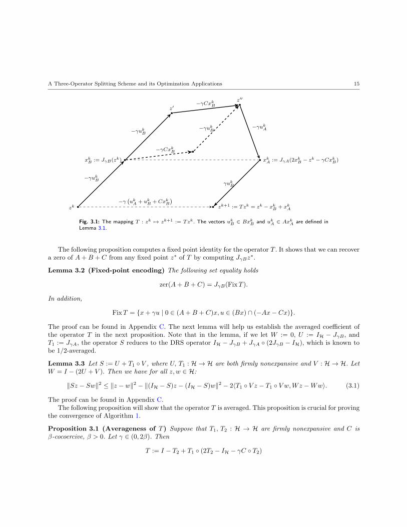
Figure 3.1 depicts the process of applying T to a point z ∈ H. Lemma 3.1 defines the points in Figure 3.1.

Lemma 3.1 Let z ∈ H and define points:

xkB := JγB(zk), z′ := 2xkB − zk, xkA := JγA(z′′),

ukB := γ−1(zk − xkB) ∈ BxkB , z′′ := z′ − γCxkB , ukA := γ−1(z′′ − xkA) ∈ AxkA.

Then the following identities hold:

Tzk − zk = xkA − xkB = −γ(ukB + ukA + CxkB) and Tzk = xkA + γukB .

When B = ∂g, we let ∇g(xkg) := ukB ∈ ∂g(xkg). Likewise when A = ∂f , we let ∇f(xkf ) := ukA ∈ ∂f(xkf ).

Proof Observe that Tzk = zk + xkA − xkB by the definition of T (Equation (1.3)). In addition, Tzk =xkA+ zk−xkB = xkA+γukB . Finally, we have xkA−xkB = 2xkB− zk−γukA−γCxkB−xkB = −γ(ukA+ukB +CxkB).

ut


zk

xkB := JγB(zk)

−γukB

z′

−γukB

−γCxkB

z′′−γCxkB

−γukB

xkA := JγA(2xkB − zk − γCxkB)

−γukA

zk+1 := Tzk = zk − xkB + xkA

γukB

−γ(ukA + ukB + CxkB

)Fig. 3.1: The mapping T : zk 7→ zk+1 := Tzk. The vectors ukB ∈ BxkB and ukA ∈ AxkA are defined inLemma 3.1.

The following proposition computes a fixed point identity for the operator T . It shows that we can recovera zero of A+B + C from any fixed point z∗ of T by computing JγBz

∗.

Lemma 3.2 (Fixed-point encoding) The following set equality holds

zer(A+B + C) = JγB(FixT ).

In addition,

FixT = x+ γu | 0 ∈ (A+B + C)x, u ∈ (Bx) ∩ (−Ax− Cx).

The proof can be found in Appendix C. The next lemma will help us establish the averaged coefficient ofthe operator T in the next proposition. Note that in the lemma, if we let W := 0, U := IH − JγB , andT1 := JγA, the operator S reduces to the DRS operator IH − JγB + JγA (2JγB − IH), which is known tobe 1/2-averaged.

Lemma 3.3 Let S := U + T1 V , where U, T1 : H → H are both firmly nonexpansive and V : H → H. LetW = I − (2U + V ). Then we have for all z, w ∈ H:

‖Sz − Sw‖2 ≤ ‖z − w‖2 − ‖(IH − S)z − (IH − S)w‖2 − 2〈T1 V z − T1 V w,Wz −Ww〉. (3.1)

The proof can be found in Appendix C.The following proposition will show that the operator T is averaged. This proposition is crucial for proving

the convergence of Algorithm 1.

Proposition 3.1 (Averageness of T ) Suppose that T1, T2 : H → H are firmly nonexpansive and C isβ-cocoercive, β > 0. Let γ ∈ (0, 2β). Then

T := I − T2 + T1 (2T2 − IH − γC T2)


is α-averaged with coefficient α := 2β4β−γ < 1. In particular, the following inequality holds for all z, w ∈ H

‖Tz − Tw‖2 ≤ ‖z − w‖2 − (1− α)

α‖(IH − T )z − (IH − T )w‖2. (3.2)

Proof To apply Lemma 3.3, we let U := IH − T2, V := 2T2 − IH − γC T2, and W := γC T2. Note that Uis firmly nonexpansive (because T2 is), and we have W = IH − (2U + V ). Let S := T = IH − T2 + T1 V .We evaluate the inner product in (3.1) as follows:

− 2〈T1 V z − T1 V w,Wz −Ww〉= 2〈(IH − T )z − (IH − T )w, γC T2z − γC T2w〉 − 2〈T2z − T2w, γC T2z − γC T2w〉

≤ ε‖(IH − T )z − (IH − T )w‖2 +γ2

ε‖C T2z − C T2w‖2 − 2γβ‖C T2z − C T2w‖2

= ε‖(IH − T )z − (IH − T )w‖2 − γ(2β − γ/ε)‖C T2z − C T2w‖2

where the inequality follows from Young’s inequality with any ε > 0 and that C is β-cocoercive. We set

ε := γ/2β < 1

so that the coefficient γ(2β − γ/ε) = 0. Now applying Lemma 3.3 and using S = T , we obtain

‖Tz − Tw‖2 ≤ ‖z − w‖2 − (1− ε)‖(IH − T )z − (IH − T )w‖2,

which is identical to (3.2) under our definition of α. utRemark 3.1 It is easy to slightly strengthen the inequality (3.2) as follows: For any ε ∈ (0, 1) and γ ∈ (0, 2βε),let α := 1/(2− ε) < 1. Then the following holds for all z, w ∈ H:

‖Tz − Tw‖2 ≤ ‖z − w‖2 − (1− α)

α‖(IH − T )z − (IH − T )w‖2

− γ(

2β − γ

ε

)‖C T2(z)− C T2(w)‖2. (3.3)

Remark 3.2 When C = 0, the mapping in Equation (1.5) reduces to S = reflγA reflγB , which is nonexpan-sive because it is the composition of nonexpansive maps. Thus, T = (1/2)IH+(1/2)S is firmly nonexpansiveby definition. However, when C 6= 0, the mapping S in (1.5) is no longer nonexpansive. The mapping2T2− IH− γC, which is a part of S, can be expansive. Indeed, consider the following example: Let H = R2,let B = ∂ι(x1,0)|x1∈R be the normal cone of the x1 axis, and let C = ∇((1/2)‖x1+x2‖2) = (x1+x2, x1+x2).In particular, T2(x1, x2) = JγB(x1, x2) = (x1, 0) for all (x1, x2) ∈ R2 and γ > 0. Then the point 0 is a fixedpoint of R = 2T2 − IH − γC T2, and

R(1, 1) = (1,−1)− γC(1, 0) = (1− γ,−1− γ).

Therefore, ‖R(1, 1)−R(0, 0)‖ =√

2 + 2γ2 >√

2 = ‖(1, 1)− (0, 0)‖ for all γ > 0.

Remark 3.3 When B = 0, the averaged parameter α = 2β/(4β − γ) in Proposition 3.1 reduces to the best(i.e., smallest) known averaged coefficient for the forward-backward splitting algorithm [19, Proposition 2.4].

We are now ready to prove convergence of Algorithm 1.


Theorem 3.1 (Main convergence theorem) Suppose that FixT 6= ∅. Set a stepsize γ ∈ (0, 2βε), whereε ∈ (0, 1). Set (λj)j≥0 ⊆ (0, 1/α) as a sequence of relaxation parameters, where α = 1/(2−ε) < 2β/(4β−γ),such that for τk := (1 − λk/α)λk/α we have

∑∞i=0 τi = ∞. Pick any start point z0 ∈ H. Let (zj)j≥0 be

generated by Algorithm 1, i.e., the following iteration: for all k ≥ 0,

zk+1 = zk + λk(Tzk − zk).

Then the following hold

1. Let z∗ ∈ FixT . Then (‖zj − z∗‖)j≥0 is monotonically decreasing.2. The sequence (‖Tzj − zj‖)j≥0 is monotonically decreasing and converges to 0.3. The sequence (zj)j≥0 weakly converges to a fixed point of T .4. Let x∗ ∈ zer(A+B + C). Suppose that infj≥0 λj > 0. Then the following sum is finite:

∞∑i=0

λk‖CxkB − Cx∗‖2 ≤1

γ(2β − γ/ε)‖z0 − z∗‖2

In particular, (CxjB)j≥0 converges strongly to Cx∗.5. Suppose that infj≥0 λj > 0 and let z∗ be the weak sequential limit of (zj)j≥0. Then the sequence (JγB(zj))j≥0

weakly converges to JγB(z∗) ∈ zer(A+B + C).6. Suppose that infj≥0 λj > 0 and let z∗ be the weak sequential limit of (zj)j≥0. Then the sequence (JγA

(2JγB − IH − γC JγB)(zj))j≥0 weakly converges to JγB(z∗) ∈ zer(A+B + C).7. Suppose that τ := infj≥0 τj > 0. For all k ≥ 0, the following convergence rates hold:

‖Tzk − zk‖2 ≤ ‖z0 − z∗‖2τ(k + 1)

and ‖Tzk − zk‖2 = o

(1

k + 1

)for any point z∗ ∈ Fix(T ).

8. Let z∗ be the weak sequential limit of (zj)j≥0. The sequences (JγB(zj))j≥0 and (JγA (2JγB − IH− γC JγB)(zj))j≥0 converge strongly to a point in zer(A+B + C) whenever any of the following holds:

(a) A is uniformly monotone3 on every nonempty bounded subset of dom(A);(b) B is uniformly monotone on every nonempty bounded subset of dom(B);(c) C is demiregular at every point x ∈ zer(A+B + C).4

Proof Part 1: Fix k ≥ 0. Observe that

‖zk+1 − z∗‖2 = ‖(1− λk)(zk − z∗) + λk(Tzk − z∗)‖2

= (1− λk)‖zk − z∗‖2 + λk‖Tzk − z∗‖2 − λk(1− λk)‖Tzk − zk‖2 (3.4)

by Corollary [3, Corollary 2.14]. In addition, from Equation (3.3), we have

‖Tzk − z∗‖2 ≤ ‖zk − z∗‖2 − 1− αα‖Tzk − zk‖2 − γ

(2β − γ

ε

)‖C T2(zk)− C T2(z∗)‖2.

3 A mapping A is uniformly monotone if there exists increasing function φ : R+ → [0,+∞] such that φ(0) = 0 and for anyu ∈ Ax and v ∈ Ay, 〈x−y, u−v〉 ≥ φ(‖x−y‖). If φ ≡ β(·)2 > 0, then the mapping A is strongly monotone. If a proper functionf is uniformly (strongly) convex, then ∂f is uniformly (strongly, resp.) monotone.

4 A mapping C is demiregular at x ∈ dom(C) if for all u ∈ Cx and all sequences (xk, uk) ∈ gra(C) with xk x and uk → u,we have xk → x.


Therefore, the monotonicity follows by combining the above two equations and using the simplification

τk = λk(1− λk) +λk(1− α)

α

to get

‖zk+1 − z∗‖2 + τk‖Tzk − zk‖2 + γλk

(2β − γ

ε

)‖CxkB − CJγB(z∗)‖2 ≤ ‖zk − z∗‖2.

Part 2: This follows from [3, Proposition 5.15(ii)].Part 3: This follows from [3, Proposition 5.15(iii)].Part 4: The inequality follows by summing the last inequality derived in Part 1. The convergence of

(CxjB)j≥0 follows because infj≥0 λj > 0 and the sum is finite.Part 5: Recall the notation from Lemma 3.1: set xkB = JγB(zk), xkA = JγA(2xkB − zk − γCxkB), ukB =

(1/γ)(zk − xkB) ∈ BxkB , and ukA = (1/γ)(2xkB − zk − γCxkB − xkA) ∈ AxkA.

Since ‖xkB − JγB(z∗)‖ = ‖JγB(zk)− JγB(z∗)‖ ≤ ‖zk − z∗‖ ≤ ‖z0 − z∗‖, ∀k ≥ 0, the sequence (xjB)j≥0 is

bounded and has a weak sequential cluster point x. Let xkjB x as j →∞ for index subsequence (kj)j≥0.

Let x∗ ∈ zer(A+B +C). Because C is maximal monotone, CxkB → Cx∗, and xkjB x, it follows by the

weak-to-strong sequential closedness of C that Cx = Cx∗ [3, Proposition 20.33(ii)] and thus CxkjB → Cx.

Because xkA − xkB = Tzk − zk → 0 as k →∞ by Part 2 and Lemma 3.1, it follows that

xkjB x, x

kjA x, Cx

kjB → Cx, u

kjB

1

γ(z∗ − x), and u

kjA

1

γ(x− z∗ − γCx)

as j →∞.

Thus, [3, Proposition 25.5] applied to (xkjA , u

kjA ) ∈ graA, (x

kjB , u

kjB ) ∈ B, and (x

kjB , Cx

kjB ) ∈ C shows that

x ∈ zer(A+B+C), z∗−x ∈ γBx, and x−z∗−γCx ∈ γAx. Hence, as x = JγB(z∗) is unique, x is the unique

weak sequential cluster point of (xjB)j≥0. Therefore, (xjB)j≥0 converges weakly to JγB(z∗) by [3, Lemma2.38].

Part 6: Assume the notation of Part 5. We shall show xkA JγB(z∗). This follows because xkA − xkB =Tzk − zk → 0 as k →∞ and xkB JγB(z∗).

Part 7: The result follows from [24, Theorem 1].Part 8: Assume the notation of Part 5 and let x∗ = JγB(z∗), u∗B = (1/γ)(z∗ − x∗) ∈ Bx∗, and u∗A =

(1/γ)(x∗ − z∗)− Cx∗. Now we move to the subcases.Part 8a: Because B+C is monotone and (xkB , u

kB) ∈ B, we have 〈xkB − x∗, ukB +CxkB − (u∗B +CxkB)〉 ≥ 0

for all k ≥ 0. Consider the bounded set S = x∗ ∪ xjA | j ≥ 0. Then there exists an increasing functionφA : R+ → [0,∞] that vanishes only at 0 such that

γφA(‖xkA − x∗‖) ≤ γ〈xkA − x∗, ukA − u∗A〉+ γ〈xkB − x∗, ukB + CxkB − (u∗B + Cx∗B)〉= γ〈xkA − xkB , ukA − u∗A〉+ γ〈xkB − x∗, ukA − u∗A〉+ γ〈xkB − x∗, ukB + CxkB − (u∗B + Cx∗B)〉= γ〈xkA − xkB , ukA − u∗A〉+ γ〈xkB − x∗, ukA + ukB + CxkB〉= 〈xkB − xkA, xkB − γukA − (x∗ − γu∗A)〉= 〈xkB − xkA, zk − z∗〉+ γ〈xkB − xkA, CxkB − Cx∗〉 → 0 as k →∞

where the convergence to 0 follows because xkB − xkA = zk − Tzk → 0, zk z∗, and CxkB → Cx∗ as k →∞.Furthermore, xkB → x∗ because xkA − xkB → 0 as k →∞.


Part 8b: Because A is monotone, we have 〈xkA − x∗, ukA − uA〉 ≥ 0 for all k ≥ 0. In addition, note that

B + C is also uniformly monotone on all bounded sets. Consider the bounded set S = x∗ ∪ xjB | j ≥ 0.Then there exists an increasing function φB : R+ → [0,∞] that vanishes only at 0 such that

φB(‖xkB − x∗‖) ≤ γ〈xkA − x∗, ukA − u∗A〉+ γ〈xkB − x∗, ukB + CxkB − (u∗B + Cx∗B)〉 → 0 as k →∞by the argument in Part 8a. Therefore, xkB → x∗ strongly.

Part 8c: Note that CxkB → Cx∗ and xkB x∗. Therefore, xkB → x∗ by the demiregularity of C. utRemark 3.4 Theorem 3.1 can easily be extended to the summable error scenario, where for all k ≥ 0, wehave

zk+1 = zk + λk(Tzk − zk + ek)

for a sequence (ej)j≥0 ⊆ H of errors that satisfy∑∞i=0 λk‖ej‖ < ∞ (e.g., using [19, Proposition 3.4]). The

result is straightforward and will only serve to complicate notation, so we omit this extension.

Remark 3.5 Note that the convergence rates for the fixed-point residual in Part 7 of Theorem 3.1 are sharp—even in the case of the variational Problem (1.2) with h = 0 [24, Theorem 8].

4 Convergence rates

In this section, we discuss the convergence rates Algorithm 1 under several different assumptions on theregularity of the problem. Section 1.2 contains a brief overview of all the convergence rates presented in thissection. For readability, we now summarize all of the convergence results of this section, briefly indicate theproof structure, and place the formal proofs in the Appendix.

4.1 General rates

We establish our most general convergence rates for the following quantities: If z∗ is a fixed point of T ,x∗ = JγB(z∗), and x ∈ H, then let

κk1(λ, x) = ‖zk − x‖2 − ‖zk+1 − x‖2 +

(1− 2

λ

)‖zk − zk+1‖2 + 2γ〈zk − zk+1, CxkB〉,

κk2(λ, x∗) = ‖zk − z∗‖2 − ‖zk+1 − z∗‖2 +

(1− 2

λ

)‖zk − zk+1‖2 + 2γ〈zk − zk+1, CxkB − Cx∗〉.

In Theorems D.1, D.2, and D.3 we deduce the following convergence rates: For j ∈ 1, 2, x1 = x, x2 = x∗

and for all k ≥ 0, we have

Nonergodic (Algorithm 1): κkj (1, xj) = o

(1 + ‖xj‖√k + 1

);

Ergodic (Algorithm 1 & (1.6)):1∑ki=0 λk

k∑i=0

κij(λi, xj) = O

(1 + ‖xj‖2k + 1

);

Ergodic (Algorithm 1 & (1.7)):2

(k + 1)(k + 2)

k∑i=0

(i+ 1)κij(λ, xj) = O

(1 + ‖xj‖2k + 1

).


It may be hard to see how these terms relate to the convergence of Algorithm 1. The key observation of Propo-sition D.2 shows that κk1 is an upper bound for a certain variational inequality associated to Problem (1.1)and that κk2 bounds the distance of the current iterate xk (or its averaged variant xk in Equations (1.6)and (1.7)) to the solution whenever one of the operators is strongly monotone.

The proofs of these convergence rates are straightforward, though technical. The nonergodic rates followfrom an application of Part 7 of Theorem 3.1, which shows that ‖zk+1 − zk‖2 = o(1/(k + 1)). The ergodicconvergence rates follow from the alternating series properties of κkj together with the summability of thegradient shown in Part 4 of Theorem 3.1.

4.2 Objective error and variational inequalities

In this section, we use the convergence rates of the upper and lower bounds derived in Theorems D.1, D.2,and D.3 to deduce convergence rates of function values and variational inequalities. All of the convergencerates have the following orders:

Nonergodic: o

(1√k + 1

)and Ergodic: O

(1

k + 1

).

The convergence rates in this section generalize some of the known convergence rates provided in [24,22,23] for Douglas-Rachford splitting, forward-Douglas-Rachford splitting, and the primal-dual forward-backward splitting, Douglas-Rachford splitting, and the proximal-point algorithms.

4.2.1 Nonergodic rates (Algorithm 1)

Suppose that A = ∂f +A, B = ∂g+B and C = ∇h+C where f, g and h are functions and A,B and C aremonotone operators. Whenever f and A are Lipschitz continuous, the following convergence rate holds:

f(xkB) + g(xkB) + h(xkB)− (f + g + h)(x) + 〈xkB − x,AxkB + ukB

+ CxkB〉 = o

(1 + ‖x‖√k + 1

). (4.1)

A more general rate holds when f and A are not necessarily Lipschitz. See Corollaries D.3 and D.4 for theexact convergence statements.

Note that quantity on the left hand side of Equation (4.1) can be negative. The point xkB is a solution tothe variational inequality problem if, and only if, the Equation (4.1) is negative for all x ∈ H, which is whywe include the dependence on ‖x‖.

Notice that when the operators A,B and C vanish and x = x∗, the convergence rate in (4.1) reduces tothe objective error of the function f + g + h at the point xkB

f(xkB) + g(xkB) + h(xkB)− (f + g + h)(x∗) = o

(1 + ‖x∗‖√k + 1

). (4.2)

and we deduce the rate o(1/√k + 1) for our method. By [24, Theorem 11], this rate is sharp.


Further nonergodic rates can be deduced whenever any A,B, or C are µA, µB and µC-strongly monotonerespectively. In particular, the following two rates hold for all k ≥ 0 Corollary D.9:

µA‖xkA − x∗‖2 + (µB + µC)‖xkB − x∗‖2 = o

(1√k + 1

);

mini=0,··· ,k

µA‖xiA − x∗‖2 + (µB + µC)‖xiB − x∗‖2

= o

(1

k + 1

).

4.2.2 Ergodic Rates

We use the same set up as Section 4.2, except we assume that A and B are skew linear mappings (i.e.,A∗ = −A and B∗ = −B) and C = 0. If (xjB)j≥0 is generated as in Equation (1.6) or Equation (1.7) and fis Lipschitz continuous, the following convergence rate holds:

f(xkB) + g(xkB) + h(xkB)− (f + g + h)(x) + 〈xkB − x,AxkB +BxkB〉 = o

(1 + ‖x‖2k + 1

). (4.3)

A more general rate holds when f is not necessarily Lipschitz. See Corollaries D.5–D.8 for the exact conver-gence statements.

Further nonergodic rates can be deduced whenever any A,B, or C are µA, µB and µC-strongly monotonerespectively. In particular, the following two rates hold for all k ≥ 0 Corollary D.9: Let (xjA)j≥0 and (xjB)j≥0

be generated by Algorithm 1 and Equations (1.6) or (1.7). Then

µA‖xkA − x∗‖2 + (µB + µC)‖xkB − x∗‖2 = O

(1

k + 1

).

4.3 Improving the objective error with Lipschitz differentiability

The worst case convergence rate o(1/√k + 1) for objective error discussed in proved in Corollary D.3 is

quite slow. Although averaging can improve the rate of convergence, this technique does not necessarilytranslate into better practical performance as discussed in Section 1.3.1. We can deduce a better rate ofconvergence for the nonergodic iterate, whenever one of the functions f or g has a Lipschitz continuousderivative. In particular, if ∇f exists and is Lipschitz, we show in Proposition D.3 that the objective errorsequence ((f+g+h)(xjB)−(f+g+h)(x∗))j≥0 is summable. From this, we immediately deduce Theorem D.5the following rate: for all k ≥ 0, we have

mini=0,··· ,k

(f + g + h)(xiB)− (f + g + h)(x∗)

= o

(1

k + 1

).

A similar result holds for the objective error sequence ((f + g + h)(xjA) − (f + g + h)(x∗))j≥0 when thefunction g is Lipschitz differentiable. Thus, when f or g is sufficiently regular, the convergence rate of thenonergodic iterate is actually faster than the convergence rate for the ergodic iterate, which motivates itsuse in practice.


4.4 Linear convergence

Whenever A,B and C are sufficiently regular, we can show that the operator T is strictly contractive towardsthe fixed point set. In particular, Algorithm 1 converges linearly whenever

(µA + µB + µC)(1/LA + 1/LB) > 0

where LA and LB are the Lipschitz constants of A and B respectively and A,B, or C are µA, µB andµC-strongly monotone respectively (where we allow the LA = LB = µA = µB = µC = 0).

Note that this linear convergence result is the best we can expect in some sense. Indeed, even if µC andµA are strongly monotone, Algorithm 1 will not necessarily converge linearly. Section D.6 we provide anexample such that

µAµC > 0, but ‖zk − z∗‖ converges arbitrarily slowly to 0.

4.5 Convergence rates for multi-block ADMM

All of the results in this section imply convergence rates for Algorithm 8, which is applied to the dualobjective in Problem (2.12). Using the techniques of [24, Section 8] and [25, Section 6], we can easily deriveconvergence rates of the primal objective in Problem (2.11). We do not pursue these results in this paperdue to lack of space.

5 Numerical results

In this section, we present some numerical examples of Algorithm 1. We emphasize that to keep our imple-mentations simple, we did not attempt to optimize the codes or their parameters for best performance. Wealso did not attempt to seriously evaluate the prediction ability of the models we tested, which is beyond thescope of this paper. Our Matlab codes will be released online on the authors’ websites. All tests were run ona PC with 32GB memory and an Intel i5-3570 CPU with Ubuntu 12.04 and Matlab R2011b installed.

5.1 Image inpainting with texture completion

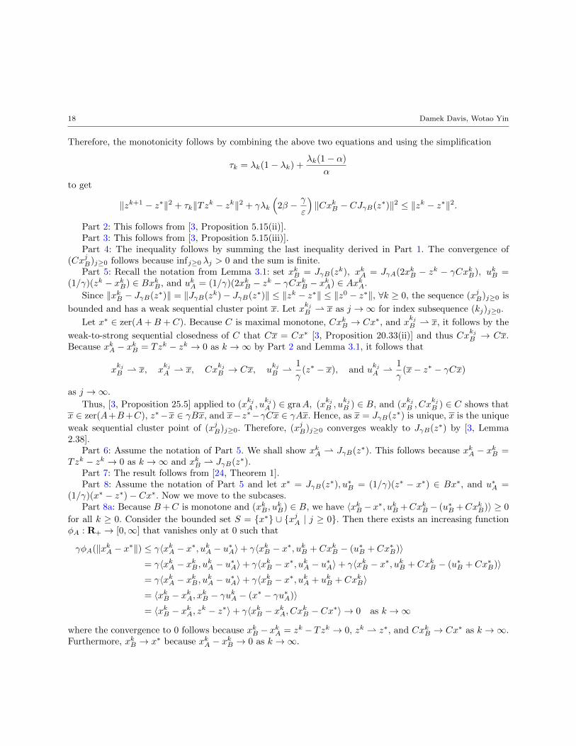
This section presents the results of applying Problem (2.8) to the color images5 of a building, parts of whichare manually occluded with white colors. See Figure 5.1. The images have a 517× 493 resolution and threecolor channels. At each iteration of Algorithm 1, the SVDs of two matrices of sizes 517×1479 and 1551×493consume most of the computing time. However, it took less 150 iterations to return good recoveries.

5 We are grateful of Professor Ji Liu for sharing his data in [33] with us.


(a) Original image (b) Occluded image 1 (c) Occluded image 2

(d) Recovered image 1 (e) Recovered image 2

Fig. 5.1: Images recovered by solving the tensor completion Problem (2.8) using Algorithm 1 for twodifferent types of occlusions.

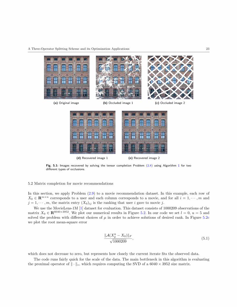
5.2 Matrix completion for movie recommendations

In this section, we apply Problem (2.9) to a movie recommendation dataset. In this example, each row ofX0 ∈ Rm×n corresponds to a user and each column corresponds to a movie, and for all i = 1, · · · ,m andj = 1, · · · ,m, the matrix entry (X0)ij is the ranking that user i gave to movie j.

We use the MovieLens-1M [1] dataset for evaluation. This dataset consists of 1000209 observations of thematrix X0 ∈ R6040×3952. We plot our numerical results in Figure 5.2. In our code we set l = 0, u = 5 andsolved the problem with different choices of µ in order to achieve solutions of desired rank. In Figure 5.2cwe plot the root mean-square error

‖A(Xkg −X0)‖F√

1000209, (5.1)

which does not decrease to zero, but represents how closely the current iterate fits the observed data.

The code runs fairly quick for the scale of the data. The main bottleneck in this algorithm is evaluatingthe proximal operator of ‖ · ‖∗, which requires computing the SVD of a 6040× 3952 size matrix.


0 20 40 60 80 100 120 140 160 180

iteration k

10−4

10−3

10−2

10−1

fixed

-poi

ntre

sidu

al

µ = 35, time = 2hr 20minµ = 40, time = 2hr 16minµ = 45, time = 2hr 7min

(a) Fixed-point residual at iteration k.

0 20 40 60 80 100 120 140 160 180

iteration k

0

50

100

150

200

250

rank


(b) Rank at iteration k.

0 20 40 60 80 100 120 140 160 180

iteration k

0.80

0.85

0.90

0.95

1.00

1.05

1.10

1.15

1.20

root

mea

nsq

uare

der

ror


(c) Root mean square error (Equation (5.1)) at iteration k.

Fig. 5.2: Run time and convergence rate statistics for the matrix completion Problem (2.9) on theMovieLens-1M database [1].

5.3 Support vector machine classification

In support vector machine classification we have a kernel matrix K ∈ Rd×d generated from a training setX = t1, · · · , td using a kernel function K : X × X → R: for all i, j = 1, · · · , d, we have Ki,j = K(ti, tj).In our particular example, X ⊆ Rn for some n > 0 and Kσ : Rn ×Rn → R++ is the Gaussian kernel given

by Kσ(t, t′) = e−σ‖t−t′‖2 for some σ > 0. We are also given a label vector y ∈ −1, 1d, which indicates the

label given to each point in X. Finally, we are given a real number C > 0 that controls how much we let ourfinal classifier stray from perfect classification on the training set X.

We define constraint sets C1 = 0 ≤ x ≤ C and C2 = x ∈ Rd | 〈y, x〉 = 0. We also define Q0 =diag(y)Kdiag(y). Then the solution to Problem (2.10) with Q = Q0 is precisely the dual form soft-marginSVM classifier [21]. Unfortunately, the Lipschitz constant of Q0 is often quite large (i.e., γ must be small),which results in poor practical performance. Thus, to improve practical we solve Problem (2.10) with Q =


C kernel parameter σ

2−5 2−3 2−1 2

1 0.82689 0.83636 0.82782 0.7755

22 0.82658 0.82441 0.81742 0.7755

24 0.83465 0.81835 0.8168 0.7755

26 0.83465 0.81835 0.80795 0.7755

Table 5.1: Classification accuracy for different choices of C and σ in the SVM model.

PC2Q0PC2 , which is equivalent to the original problem because the minimizer must lie in C2. The result is amuch smaller Lipschitz constant for Q and better practical performance. This trick was first reported in [23,Section 1.6].

We evaluated our algorithm on a subsetXall of the UCI “Adult” machine learning dataset which is entitled“a7a” and is available from the LIBSVM website [13]. Our training set Xtrain consisted of a d = 9660 elementsubsample of this 16100 element training set (i.e., a 60% sample). Note that Q has d2 = 96602 = 93315600nonzero entries. In table 5.1, we trained the SVM model (2.10) with different choices of parameters Cand σ, and then evaluated their prediction accuracy on the remaining 16100 − 9660 = 6440 elements inXtest = Xall\Xtrain. We found that the parameters σ = 2−3 and C = 1 gave the best performance on thetest set, so we set these to be the parameters for our numerical experiments.

Figure 5.3 plots the results of our test. Figures 5.3a and 5.3b compare the line search method in Al-gorithm 3 with the basic Algorithm 1. We see that the line search method performs better than the basicalgorithm in terms of number of iterations and total CPU time needed to reach a desired accuracy. Becauseof the linearity of the projection PC2 , we can find a closed form solution for the line search weight ρ inAlgorithm 5.3a as the root of a third degree polynomial. Thus, although Algorithm 3 requires more work periteration than Algorithm 1, it still takes less time overall because Algorithm 1 must compute β = 1/‖Q‖,which is quite costly.

Finally, in Figure 5.3c we compare the performance of the nonergodic iterate generated by Algorithm 1,the standard ergodic iterate (1.6), and the newly introduced ergodic iterate (1.7). We see that the nonergodiciterate performs better than the other two, and as expected, the the new ergodic iterate outperforms thestandard ergodic iterate. We emphasize that computing these iterates is essentially costless for the user andonly modifies the final output of the algorithm, not the trajectory.

We emphasize that all steps in this algorithm can be computed in closed form, so implementation is easyand each iteration is quite cheap.

5.4 Portfolio optimization

In this section, we evaluate our algorithm on the portfolio optimization problem. In this problem, we havea choice to invest in d > 0 assets and our goal is to choose how to distribute our resources among all theassets so that we minimize investment risk, and guarantee that our expected return on the investments isgreater than r ≥ 0. Mathematically, we model the distribution of our assets with a vector x ∈ Rd where xirepresents the percentage of our resources that we invest in asset i. For this reason, we define our constraintset C1 = x ∈ Rd | ∑n

i=1 xi = 1, xi ≥ 0 to be the standard simplex. We also assume that we are given


0 200 400 600 800 1000

iteration k

10−5

10−4

10−3

10−2

10−1

100

101

fixed

-poi

ntre

sidu

al

γ = 0.1250, time = 388s, LSγ = 0.0049, time = 976s

(a) Fixed-point residual with and without line search (LS).

0 50 100 150 200 250 300 350 400

iteration k

−3000

−2500

−2000

−1500

−1000

−500

0

obje

ctiv

eva

lue

γ = 0.1250, time = 388s, LSγ = 0.0049, time = 976s

(b) Objective value with and without line search (LS).

0 200 400 600 800 1000

iteration k

−3000

−2500

−2000

−1500

−1000

−500

0

obje

ctiv

eva

lue

γ = 0.0049, nonergodicγ = 0.0049, ergodic standardγ = 0.0049, ergodic new

(c) Comparison of ergodic and nonergodic iterates.

Fig. 5.3: Run time and convergence rate statistics for the SVM Problem (2.10) on the UCI “Adult” Machinelearning dataset [30]. Results are with the parameter choice that has the best generalization to the test set(C, σ) = (1, 0.2−3).

a vector of mean returns m ∈ Rd where mi represents the expected return from asset i, and we defineC2 = x ∈ Rd | 〈m,x〉 ≥ r. Typically, we model the risk with a matrix Q0 ∈ Rd×d, which is usually chosenas the covariance matrix of asset returns. However, we stray from the typical model by setting Q = Q0 +µIRd

for some µ ≥ 0, which has the effect of encouraging diversity of investments among the assets. In order tochoose our optimal investment strategy, we solve Problem (2.10) with Q, C1 and C2 introduced here.

In our numerical experiments, we solve a d = 1000 dimensional portfolio optimization problem with arandomly generated covariance matrix Q0 (using the Matlab “gallery” function) and mean return vector m.We report our results in Figure 5.4. In order to get an estimate of the solution of Problem (2.10), we firstsolved this problem to high-accuracy using an interior point solver.

The matrix Q in this example is positive definite for any choice of µ ≥ 0, but the condition number ofQ0 is around 8000, while the condition number of Q with µ = .1 is around 5. For this reason, we see a huge


0 50 100 150 200 250 300 350 400

iteration k

10−6

10−5

10−4

10−3

10−2

10−1

100

dist

ance

toop

tim

alit

y

Accelerated, µ = .1

Standard, µ = .1

(a) Distance to solution using accelerated and non acceler-ated methods.

0 50 100 150 200

iteration k

10−5

10−4

obje

ctiv

eva

lue

Accelerated, µ = 0

Standard, µ = 0

CVX optimal

(b) Objective value of accelerated and non accelerated meth-ods. The blue curve is covered by the blue curve.

Fig. 5.4: Convergence rate statistics for the portfolio optimization problem in Section 5.4.

improvement in Figure 5.4a with the acceleration in Algorithm 2, while in the case µ = 0 in Figure 5.4b, theaccelerated and non accelerated versions are nearly identical.

We emphasize that all steps in this algorithm can be computed in nearly closed form, so implementationis easy and each iteration is quite cheap.

6 Conclusion

In this paper, we introduced a new operator-splitting algorithm for the three-operator monotone inclusionproblem, which has a large variety of applications. We showed how to accelerate the algorithm wheneverone of the involved operators is strongly monotone, and we also introduced a line search procedure andtwo averaging strategies that can improve the convergence rate. We characterized the convergence rate ofthe algorithm under various scenarios and showed that many of our rates are sharp. Finally, we introducednumerous applications of the algorithm and showed how it unifies many existing splitting schemes.

References

1. MovieLens. http://grouplens.org/datasets/movielens/. Accessed: 2015-01-32. Bauschke, H.H., Bello Cruz, J.Y., Nghia, T.T.A., Phan, H.M., Wang, X.: The rate of linear convergence of the Douglas-

Rachford algorithm for subspaces is the cosine of the Friedrichs angle. Journal of Approximation Theory 185(0), 63–79(2014)

3. Bauschke, H.H., Combettes, P.L.: Convex Analysis and Monotone Operator Theory in Hilbert Spaces, 1st edn. SpringerPublishing Company, Incorporated (2011)

4. Bot, R.I., Csetnek, E.R.: On the convergence rate of a forward-backward type primal-dual splitting algorithm for convexoptimization problems. Optimization 64(1), 5–23 (2015)

5. Bot, R.I., Csetnek, E.R., Heinrich, A., Hendrich, C.: On the convergence rate improvement of a primal-dual splittingalgorithm for solving monotone inclusion problems. Mathematical Programming pp. 1–29 (2014)

6. Bot, R.I., Hendrich, C.: A Douglas–Rachford type primal-dual method for solving inclusions with mixtures of compositeand parallel-sum type monotone operators. SIAM Journal on Optimization 23(4), 2541–2565 (2013)

http://grouplens.org/datasets/movielens/


7. Bot, R.I., Hendrich, C.: Solving monotone inclusions involving parallel sums of linearly composed maximally monotoneoperators. arXiv preprint arXiv:1306.3191v2 (2013)

8. Briceno-Arias, L.M., Combettes, P.L.: A Monotone+Skew Splitting Model for Composite Monotone Inclusions in Duality.SIAM Journal on Optimization 21(4), 1230–1250 (2011)

9. Briceno-Arias, L.M.: Forward-Douglas-Rachford splitting and forward-partial inverse method for solving monotone inclu-sions. Optimization, to appear pp. 1–23 (2013)

10. Cai, X., Han, D., Yuan, X.: The direct extension of ADMM for three-block separable convex minimization models isconvergent when one function is strongly convex. Optimization Online (2014)

11. Candes, E., Plan, Y.: Matrix Completion With Noise. Proceedings of the IEEE 98(6), 925–936 (2010)12. Chambolle, A., Pock, T.: A First-Order Primal-Dual Algorithm for Convex Problems with Applications to Imaging. Journal

of Mathematical Imaging and Vision 40(1), 120–145 (2011)13. Chang, C.C., Lin, C.J.: LIBSVM: A library for support vector machines. ACM Transactions on Intelligent Systems and

Technology 2, 27:1–27:27 (2011). Software available at http://www.csie.ntu.edu.tw/~cjlin/libsvm

14. Chen, C., He, B., Ye, Y., Yuan, X.: The direct extension of admm for multi-block convex minimization problems isnot necessarily convergent. Mathematical Programming pp. 1–23 (2014). DOI 10.1007/s10107-014-0826-5. URL http:

//dx.doi.org/10.1007/s10107-014-0826-5

15. Chen, C., Shen, Y., You, Y.: On the Convergence Analysis of the Alternating Direction Method of Multipliers with ThreeBlocks. Abstract and Applied Analysis 2013, e183,961 (2013)

16. Combettes, P.L.: Systems of Structured Monotone Inclusions: Duality, Algorithms, and Applications. SIAM Journal onOptimization 23(4), 2420–2447 (2013)

17. Combettes, P.L., Condat, L., Pesquet, J.C., Vu, B.C.: A Forward-Backward View of Some Primal-Dual OptimizationMethods in Image Recovery. In: IEEE International Conference on Image Processing. Paris, France (2014)

18. Combettes, P.L., Pesquet, J.C.: Primal-Dual Splitting Algorithm for Solving Inclusions with Mixtures of Composite, Lips-chitzian, and Parallel-Sum Type Monotone Operators. Set-Valued and Variational Analysis 20(2), 307–330 (2012)

19. Combettes, P.L., Yamada, I.: Compositions and convex combinations of averaged nonexpansive operators. Journal ofMathematical Analysis and Applications 425(1), 55–70 (2015)

20. Condat, L.: A Primal–Dual Splitting Method for Convex Optimization Involving Lipschitzian, Proximable and LinearComposite Terms. Journal of Optimization Theory and Applications 158(2), 460–479 (2013)

21. Cortes, C., Vapnik, V.: Support-vector networks. Mach. Learn. 20(3), 273–297 (1995)22. Davis, D.: Convergence rate analysis of primal-dual splitting schemes. arXiv preprint arXiv:1408.4419v2 (2014)23. Davis, D.: Convergence rate analysis of the forward-douglas-rachford splitting scheme. arXiv preprint arXiv:1410.2654v3

(2014)24. Davis, D., Yin, W.: Convergence rate analysis of several splitting schemes. arXiv preprint arXiv:1406.4834v2 (2014)25. Davis, D., Yin, W.: Faster convergence rates of relaxed Peaceman-Rachford and ADMM under regularity assumptions.

arXiv preprint arXiv:1407.5210v2 (2014)26. Esser, E., Zhang, X., Chan, T.F.: A General Framework for a Class of First Order Primal-Dual Algorithms for Convex

Optimization in Imaging Science. SIAM Journal on Imaging Sciences 3(4), 1015–1046 (2010)27. Han, D., Yuan, X.: A Note on the Alternating Direction Method of Multipliers. Journal of Optimization Theory and

Applications 155(1), 227–238 (2012)28. Komodakis, N., Pesquet, J.C.: Playing with Duality: An Overview of Recent Primal-Dual Approaches for Solving Large-

Scale Optimization Problems. arXiv preprint arXiv:1406.5429v2 (2014)29. Li, M., Sun, D., Toh, K.C.: A Convergent 3-Block Semi-Proximal ADMM for Convex Minimization Problems with One

Strongly Convex Block. arXiv:1410.7933 [math] (2014)30. Lichman, M.: UCI machine learning repository (2013). URL http://archive.ics.uci.edu/ml

31. Lin, T., Ma, S., Zhang, S.: On the Convergence Rate of Multi-Block ADMM. arXiv:1408.4265 [math] (2014)32. Lions, P.L., Mercier, B.: Splitting Algorithms for the Sum of Two Nonlinear Operators. SIAM Journal on Numerical

Analysis 16(6), 964–979 (1979)33. Liu, J., Musialski, P., Wonka, P., Ye, J.: Tensor completion for estimating missing values in visual data. IEEE Transactions

on Pattern Analysis and Machine Intelligence 35(1), 208–220 (2013)34. Nedich, A., Lee, S.: On Stochastic Subgradient Mirror-Descent Algorithm with Weighted Averaging. SIAM Journal on

Optimization 24(1), 84–107 (2014)35. Nesterov, Y.: Introductory Lectures on Convex Optimization: A Basic Course, Applied Optimization, vol. 87. Springer

(2004)36. Passty, G.B.: Ergodic Convergence to a Zero of the Sum of Monotone Operators in Hilbert Space. Journal of Mathematical

Analysis and Applications 72(2), 383–390 (1979)37. Pock, T., Cremers, D., Bischof, H., Chambolle, A.: An algorithm for minimizing the mumford-shah functional. In: Computer

Vision, 2009 IEEE 12th International Conference on, pp. 1133–1140. IEEE (2009)

http://www.csie.ntu.edu.tw/~cjlin/libsvm

http://dx.doi.org/10.1007/s10107-014-0826-5

http://dx.doi.org/10.1007/s10107-014-0826-5

http://archive.ics.uci.edu/ml


38. Tseng, P.: A Modified Forward-Backward Splitting Method for Maximal Monotone Mappings. SIAM Journal on Controland Optimization 38(2), 431–446 (2000)

39. Vu, B.C.: A splitting algorithm for dual monotone inclusions involving cocoercive operators. Advances in ComputationalMathematics 38(3), 667–681 (2013)

A Proof of Theorem 1.2

We first prove a useful inequality.

Proposition A.1 Let B be µB-strongly monotone where we allow the case µB = 0. Suppose that x0A ∈ H and set x0B =Jγ0B(x0A), u0B = (1/γ0)(I − JγB)(x0A). For all k ≥ 0, let

xk+1B = JγkB(xkA + γku

kB);

uk+1B = (1/γk)(xkA + γku

kB − x

k+1B );

xk+1A = Jγk+1A(xk+1

B − γk+1uk+1B − γk+1Cx

k+1B ).

(A.1)

1. Suppose that C is β-cocoercive and µC-strongly monotone. Let η ∈ (0, 1) and let (γj)j≥0 ⊆ (0, 2(1 − η)β). Then thefollowing inequality holds for all k ≥ 0:

(1 + 2γkµB)‖xk+1B − x∗‖2 + γ2k‖uk+1

B − u∗B‖2 +

(1− γk

2(1− η)β

)‖xkA − xkB‖2

≤ (1− 2γkµCη)‖xkB − x∗‖2 + γ2k‖ukB − u∗B‖2. (A.2)

2. Suppose that C is LC-Lipschitz, but not necessarily strongly monotone. In addition, suppose that µB > 0. Then thefollowing inequality holds for all k ≥ 0:

(1 + 2γk(µB − γkL2C/2))‖xk+1

B − x∗‖2 + γ2kL2C‖xk+1

B − x∗‖2 + γ2k‖uk+1B − u∗B‖2

≤ ‖xkB − x∗‖2 + γ2kL2C‖xkB − x∗‖2 + γ2k‖ukB − u∗B‖2. (A.3)

Proof Fix k ≥ 0.

Part 1: Following Fig. 3.1 and Lemma 3.1, let

ukA =1

γk((xkB − γkukB − γkCxkB)− JγkA(xkB − γkukB − γkCxkB)) ∈ AukA.

In addition, ukB ∈ BukB for all k ≥ 0. The following identities from Fig. 3.1 will be useful in the proof:

xkA − xk+1B = γk(uk+1

B − ukB)

xkB − xk+1B = γk(uk+1

B + CxkB + ukA)

xkB − xkA = γk(ukB + CxkB + ukA).


First we bound the sum of two inner product terms.

2γk

(〈xkA − x∗, ukA + CxkB〉+ 〈xk+1

B − x∗, uk+1B 〉

)= 2γk

(〈xkA − xk+1

B , ukA + CxkB〉+ 〈xk+1B − x∗, uk+1

B + ukA + CxkB〉)

= 2γk

(〈xkA − xk+1

B , ukA + CxkB + ukB〉+ 〈xkA − xk+1B , ukB〉

)+ 2〈xk+1

B − x∗, xkB − xk+1B 〉

= 2〈xkA − xk+1B , xkB − xkA〉+ 2〈xk+1

B − x∗, xkB − xk+1B 〉+ 2γk〈xkA − xk+1

B , ukB − u∗B〉+ 2γk〈xkA − xk+1

B , u∗B〉= ‖xkB − xk+1

B ‖2 − ‖xkA − xk+1B ‖2 − ‖xkA − xkB‖2

+ ‖xkB − x∗‖2 − ‖xk+1B − x∗‖2 − ‖xkB − xk+1

B ‖2

+ 2γ2k〈ukB − uk+1B , ukB − u∗B〉+ 2γk〈xkA − xk+1

B , u∗B〉= ‖xkB − x∗‖2 − ‖xk+1

B − x∗‖2 − ‖xkA − xk+1B ‖2 − ‖xkA − xkB‖2

+ γ2k

(‖ukB − u∗B‖2 − ‖uk+1

B − u∗B‖2 + ‖ukB − uk+1B ‖2

)+ 2γk〈xk+1

B − xkA, u∗B〉

= ‖xkB − x∗‖2 − ‖xk+1B − x∗‖2 − ‖xkA − xkB‖2

+ γ2k‖ukB − u∗B‖2 − γ2k‖uk+1B − u∗B‖2 + 2γk〈xk+1

B − xkA, u∗B〉. (A.4)

Furthermore, we have the lower bound

2γk


B − x∗, uk+1B 〉

)≥ 2γk

(〈xkA − x∗, u∗A + CxkB〉+ 〈xk+1

B − x∗, u∗B〉)

+ 2γkµB‖xk+1B − x∗‖2. (A.5)

We have the further lower bound: For all η ∈ (0, 1), we have

2〈xkA − x∗, CxkB〉 = 2〈xkA − xkB , CxkB − Cx∗〉+ 2〈xkA − xkB , Cx∗〉+ 2〈xkB − x∗, CxkB〉

≥ − 1

2β(1− η)‖xkA − xkB‖2 − 2β(1− η)‖CxkB − Cx∗‖2 + 2µCη‖xkB − x∗‖2

+ 2β(1− η)‖CxkB − Cx∗‖2 + 2〈xkA − x∗, Cx∗〉. (A.6)

Altogether, we have

2γk


B − x∗, uk+1B 〉

)≥ 2γk

(〈xkA − x∗, u∗A + Cx∗〉+ 〈xk+1

B − x∗, u∗B〉)

− γk

2(1− η)β‖xkA − xkB‖2 + 2γkµC(1− η)‖xkB − x∗‖2 + 2γkµB‖xk+1

B − x∗‖2

= 2γk〈xk+1B − xkA, u∗B〉 −

γk

2(1− η)β‖xkA − xkB‖2 + 2γkµCη‖xkB − x∗‖2 + 2γkµB‖xk+1

B − x∗‖2. (A.7)

Thus, combine (A.4) and (A.7) to get

(1 + 2γkµB)‖xk+1B − x∗‖2 + γ2k‖uk+1

B − u∗B‖2 +

(1− γk

2(1− η)β

)‖xkA − xkB‖2

≤ (1− 2γkµCη)‖xkB − x∗‖2 + γ2k‖ukB − u∗B‖2.Part 2: This follows the exact same reasoning, except we replace Equation (A.6) with the following lower bound:

2〈xkA − x∗, CxkB〉 = 2〈xkA − xkB , CxkB − Cx∗〉+ 2〈xkA − xkB , Cx∗〉+ 2〈xkB − x∗, CxkB〉

≥ − 1

γk‖xkA − xkB‖2 − γk‖CxkB − Cx∗‖2 + 2〈xkA − x∗, Cx∗〉

≥ − 1

γk‖xkA − xkB‖2 − γkL2

C‖xkB − x∗‖2 + 2〈xkA − x∗, Cx∗〉.


ut

We are now ready to prove Theorem 1.2.

Proof (Theorem 1.2) Part 1: The definition of γk+1 ensures that

1 + 2γkµB

γ2k=

(1− 2γk+1µCη)

γ2k+1

.

Therefore, by (A.2), the following inequality holds for all k ≥ 0:

(1− γk+1µCη)

γ2k+1

‖xk+1B − x∗‖2 + ‖uk+1

B − u∗B‖2 ≤(1− γkµCη)

γ2k‖xkB − x∗‖2 + ‖ukB − u∗B‖2.

Now observe that from Equation (1.8), we have γk → 0 as k →∞. Therefore,

γk

γk+1=

√1 + 2γkµB

1− 2γk+1µCη→ 1 as k →∞.

In addition, the sequence (1/γj)j≥0 is increasing:

γ2k − γ2k+1 = γkγk+1 (2γkµB + 2γk+1µCη) > 0.

Thus, we apply the Stolz-Cesaro theorem to compute the following limit:

limk→∞

(k + 1)γk = limk→∞

k + 11γk

= limk→∞

(k + 2)− (k + 1)1

γk+1− 1γk

= limk→∞

γkγk+1

γk − γk+1= limk→∞

γkγk+1(γk+1 + γk)

γ2k − γ2k+1

= limk→∞


γkγk+1(2γkµB + 2γk+1µCη)= limk→∞

1 + γkγk+1

2 γkγk+1

µB + 2µCη= limk→∞

1 + γkγk+1

2 γkγk+1

µB + 2µCη

=1

µCη + µB.

Thus, we have

‖xk+1B − x∗‖2 ≤

γ2k+1

(1− γk+1µCη)

((1− γ0µCη)

γ20‖x0B − x∗‖2 + ‖u0B − u∗B‖2

)= O

(1

(k + 1)2

).

Part 2: The proof is nearly identical to the proof of Part 1. The difference is that the definition of γk+1 ensures that for allk ≥ 0, we have

1

γ2k+1

=(1 + 2γk(µB − γkL2

C/2))

γ2k.

In addition, we have γk → 0 as k →∞. The sequence (1/γj)j≥0 is also increasing because γk < 2L2C/µB for all k ≥ 0. Finally

we note that γk/γk+1 → 1 as k →∞. Thus, we apply the Stolz-Cesaro theorem to compute the following limit:

limk→∞

(k + 1)γk = limk→∞

k + 11γk

= limk→∞

(k + 2)− (k + 1)1

γk+1− 1γk

= limk→∞

γkγk+1

γk − γk+1= limk→∞


γ2k − γ2k+1

= limk→0


2γ2k+1γk(µB − γkL2C/2)

= limk→0

γk+1 + γk

γk+1(2µB − γkL2C)

= limk→0

1 + γk/γk+1

2µB − γkL2C

=1

µB.

ut


B Derivation of Algorithm 11

Observe the following identities from Fig. 3.1 and Lemma 3.1:

xkA − xk+1B = γ(uk+1

B − ukB); (B.1a)

xkB − xk+1B = γ(uk+1

B + CxkB + ukA); (B.1b)

xkB − xkA = γ(ukB + CxkB + ukA). (B.1c)

These give us the further subgradient identity:

uk+1A = ukA + (uk+1

A + uk+1B + Cxk+1

B ) + (CxkB − Cxk+1B )− (ukA + uk+1

B + CxkB)

= ukA +1

γ(xk+1B − xk+1

A ) + (CxkB − Cxk+1B ) +

1

γ(xk+1B − xkB)

= J 1γA−1

(ukA +

1

γ(2xk+1

B − xkB) + (CxkB − Cxk+1B )

),

where the first equality follows from cancellation, the second from (B.1), and the third from the property:

for any v ∈ H, uk+1A = v − 1

γxk+1A , (xk+1

A , uk+1A ) ∈ graA ⇐⇒ uk+1

A = J 1γA−1 (v),

which follows from the definition of resolvent J 1γA−1 . In addition,

xk+1B = xkB − γ(uk+1

B + CxkB + ukA)

= JγB

(xkB − γCxkB − γukA

),

where the second equality follows from the property

for any v ∈ H, xk+1B = v − γuk+1

B , (xk+1B , uk+1

B ) ∈ graB ⇐⇒ xk+1B = JγB(v).

Altogether, for all k ≥ 0, we have

xk+1B = JγB

(xkB − γCxkB − γukA

),

uk+1A = J 1

γA−1

(ukA +

1

γ(2xk+1

B − xkB) + (CxkB − Cxk+1B )

).

Algorithm 11 is obtained with the change of variable: xk ← xkB and yk ← ukA.

C Proofs from Section 3

Proof (of Lemma 3.2) Let x ∈ zer(A + B + C), that is, 0 ∈ (A + B + C)x. Let uA ∈ Ax and uB ∈ Bx be such thatthat uA + uB + Cx = 0. In addition, let z = x + γuB . We will show that z is a fixed point of T . Then JγB(z) = x and2JγB(z)−z−γCJγB(z) = 2x−z−γCx = x−γCx−γuB = x+γuA. Thus, x = JγA(x+γuA) = JγA(2JγB(z)−z−γCJγB(z)).Therefore,

Tz = T (x+ γuB)

= JγA(2JγB(z)− z − γCJγB(z)) + (IH − JγB)(z)

= x+ γuB

= z.


Next, suppose that z ∈ FixT . Then there exists uB ∈ B(JγB(z)) and uA ∈ A(JγA(2JγB(z)− z − γCJγB(z))) such that

z = Tz

= z + JγA(2JγB(z)− z − γCJγB(z))− JγB(z)

= z − γ(uA + uB + CJγB(z)).

Thus, x = JγA(2JγB(z)− z − γCJγB(z)) = JγB(z) and uA + uB + Cx = 0. Therefore, x = JγB(z) ∈ zer(A+B + C).The identity for FixT immediately follows from the fixed-point construction process in the first paragraph. ut

Proof (of Lemma 3.3) Let z, w ∈ H. Then

‖Sz − Sw‖2 = ‖Uz − Uw‖2 + ‖T1 V z − T1 V w‖2 + 2〈T1 V z − T1 V w,Uz − Uw〉≤ 〈Uz − Uw, z − w〉+ 〈T1 V z − T1 V w, V z − V w〉+ 2〈T1 V z − T1 V w,Uz − Uw〉= 〈Uz − Uw, z − w〉+ 〈T1 V z − T1 V w, (2U + V )z − (2U + V )w〉= 〈Uz − Uw, z − w〉+ 〈T1 V z − T1 V w, (I −W )z − (I −W )w〉= 〈Sz − Sw, z − w〉 − 〈T1 V z − T1 V w,Wz −Ww〉

where the inequality follows from the firm nonexpansiveness of U and T1. Then, the result follows from the identity:

〈Sz − Sw, z − w〉 =1

2‖z − w‖2 − 1

2‖(IH − S)z − (IH − S)w‖2 +

1

2‖Sz − Sw‖2.

ut

D Proofs for convergence rate analysis

We now recall a lower bound property for convex functions that are strongly convex and Lipschitz differentiable. The first boundis a consequence of [3, Theorem 18.15] and the second bound is a combination of [3, Theorem 18.15] and [35, Theorem 2.1.12].

Proposition D.1 Suppose that f : H → (0,∞] is µ-strongly convex and (1/β)-Lipschitz differentiable. For all x, y ∈ dom(f),let

Sf (x, y) := max

β

2‖∇f(x)−∇f(y)‖2, µ

2‖x− y‖2

(D.1)

Qf (x, y) := max

2Sf (x, y),

µ

(µβ + 1)‖x− y‖2 +

β

(µβ + 1)‖∇f(x)−∇f(y)‖2

. (D.2)

Then for all x, y ∈ dom(f), we have

f(x)− f(y)− 〈x− y,∇f(y)〉 ≥ Sf (x, y); (D.3)

〈∇f(x)−∇f(y), x− y〉 ≥ Qf (x, y). (D.4)

Similarly, if A : H → H is µ-strongly monotone and β-cocoercive, we let

QA(x, y) = maxµ‖x− y‖2, β‖Ax−Ay‖2

for all x, y ∈ dom(A). Then for all x, y ∈ dom(A), we have

〈Ax−Ay, x− y〉 ≥ QA(x, y).

We follow the convention that every function f is µf ≥ 0 strongly convex and (1/βf ) ≥ 0 Lipschitz where we allowthe possibility that βf = µf = 0. With this notation, the results of Proposition D.1 continue hold for all f . We follow the

same convention for monotone operators. In particular, every monotone operator A : H → 2H is µA-strongly monotone andβA-cocoercive where µA ≥ 0 and βA ≥ 0. Finally, we follow convention that Q∂f := Qf .

Note that we could extend our definition of QA(·, ·) (or Qf (·, ·)) to the case where A is merely strongly monotone in asubset of the coordinates of H (which is then assumed to be a product space). This extension is straightforward, though slightlymessy. Thus, we omit this extension.

The following identity will be applied repeatedly:


Proposition D.2 Let z ∈ H, let z∗ be a fixed point of T , let γ > 0, let λ > 0, and let z+ = (1− λ)z + λTz. Then

2γλ〈xB − xA, u∗B + Cx∗〉+ 2γλQA(xA, x∗) + 2γλQB(xB , x

∗) + 2γλQC(xB , x∗)

≤ 2γλ〈xA − x∗, uA〉+ 2γλ〈xB − x∗, uB + CxB〉 (D.5)

= ‖z − x∗‖2 − ‖z+ − x∗‖2 +

(1− 2

λ

)‖z − z+‖2 + 2γ〈z − z+, CxB〉 (D.6)

= ‖z − z∗‖2 − ‖z+ − z∗‖2 +

(1− 2

λ

)‖z − z+‖2 + 2γ〈z − z+, CxB + u∗B〉 (D.7)

where xA ∈ dom(A), xB ∈ dom(B), uB ∈ BxB and uA ∈ AuA are defined in Lemma 3.1 and Equation (D.6) holds for allx∗ ∈ H, while Equations (D.5) and (D.7) hold when x∗ = JγB(z∗) and u∗B = 1

γ(z∗ − x∗). In particular, when x∗ = JγB(z∗),

we have

‖z+ − z∗‖2 +

(2

λ− 1

)‖z − z+‖2 + 2γλQA(xA, x

∗) + 2γλQB(xB , x∗) + 2γλQC(xB , x

∗)

≤ ‖z − z∗‖2 + 2γ〈z − z+, C(xB)− C(x∗)〉. (D.8)

Proof First we show inequality (D.5): Let u∗A ∈ Ax∗ and u∗B ∈ Bx∗ be such that u∗A + u∗B + Cx∗ = 0. Then

2γλ〈xA − x∗, uA〉+ 2γλ〈xB − x∗, uB + CxB〉≥ 2γλ〈xA − x∗, u∗A〉+ 2γλ〈xB − x∗, u∗B + Cx∗〉+ 2γλQA(xA, x


∗)

= γλ〈xA − x∗, u∗A + u∗B + Cx∗〉+ 2γλ〈xB − xA, u∗B + Cx∗〉+ 2γλQA(xA, x∗) + 2γλQB(xB , x

∗) + 2γλQC(xB , x∗)

= 2γλ〈xB − xA, u∗B + Cx∗〉+ 2γλQA(xA, x∗) + 2γλQB(xB , x

∗) + 2γλQC(xB , x∗).

Now we show Equation (D.6):

2λγ〈xA − x∗, uA〉+ 2γλ〈xB − x∗, uB + CxB〉= 2γλ〈xA − xB , uA〉+ 2γλ〈xB − x∗, uA + uB + CxB〉= 2λ〈xA − xB , γuA〉+ 2λ〈xB − x∗, xB − xA〉= 2λ〈xB − γuA − x∗, xB − xA〉= 2〈z + (xB − z − γuA)− x∗, z − z+〉= 2〈z − γ(uB + uA + CxB)− x∗, z − z+〉+ 2γ〈z − z+, CxB〉

= 2〈z − 1

λ(z − z+)− x∗, z − z+〉+ 2γ〈z − z+, CxB〉

= 2〈z − x∗, z − z+〉 − 2

λ‖z − z+‖2 + 2γ〈z − z+, CxB〉

(1.12)= ‖z − x∗‖2 − ‖z+ − z∗‖2 +

(1− 2

λ

)‖z − z+‖2 + 2γ〈z − z+, CxB〉.

Now assume that x∗ = JγB(z∗) and show Equation (D.7):

2λγ〈xA − x∗, uA〉+ 2γλ〈xB − x∗, uB + CxB〉

= 2〈z − x∗, z − z+〉 − 2

λ‖z − z+‖2 + 2γ〈z − z+, CxB〉

= 2〈z − z∗, z − z+〉 − 2

λ‖z − z+‖2 + 2γ〈z − z+, CxB + u∗B〉

(1.12)= ‖z − z∗‖2 − ‖z+ − z∗‖2 +

(1− 2

λ

)‖z − z+‖2 + 2γ〈z − z+, CxB + u∗B〉.

Equation (D.8) follows from rearranging the above inequalities. ut


Corollary D.1 (Function value bounds) Assume the notation of Proposition D.2. Let f, g, and h be closed, proper andconvex functions from H to (−∞,∞]. Suppose that h is (1/β)-Lipschitz differentiable. Suppose that A = ∂f , B = ∂g, and

C = ∇h. Then if x∗ = proxγg(z∗), ∇g(x∗) = (1/γ)(z∗ − x∗), and ∇f(x∗) ∈ ∂f(x∗) and ∇g(x∗) ∈ ∂g(x∗) are such that

∇h(x∗) + ∇g(x∗) + ∇f(x∗) = 0, we have

2γ〈z − z+, ∇g(x∗) +∇h(x∗)〉+ 4γλSf (xf , x∗) + 4γλSg(xg , x

∗) + 4γλSh(xg , x∗)

≤ 2γλ(f(xf ) + g(xg) + h(xg)− (f + g + h)(x∗) + Sf (xf , x

∗) + Sg(xg , x∗) + Sh(xg , x

∗))

(D.9)

≤ ‖z − x∗‖2 − ‖z+ − x∗‖2 +

(1− 2

λ

)‖z − z+‖2 + 2γ〈z − z+,∇h(xB)〉 (D.10)

= ‖z − z∗‖2 − ‖z+ − z∗‖2 +

(1− 2

λ

)‖z − z+‖2 + 2γ〈z − z+,∇h(xB) + ∇g(x∗)〉. (D.11)

where xf ∈ dom(f), xg ∈ dom(g) are defined in Lemma 3.1 and Equation (D.10) holds for all x∗ ∈ H, while Equations (D.9)

and (D.11) hold when x∗ = proxγg(z∗) and ∇g(x∗) = 1γ

(z∗ − x∗). In particular, when x∗ = proxγg(z∗), we have

‖z+ − z∗‖2 +

(2

λ− 1

)‖z − z+‖2 + 4γλSf (xf , x

∗) + 4γλSg(xg , x∗) + 4γλSh(xg , x

∗)

≤ ‖z − z∗‖2 + 2γ〈z − z+,∇h(xB)−∇h(x∗)〉. (D.12)

Proof Equation (D.11) is a direct consequence of Proposition D.2 together with the inequalities:

f(xf ) + g(xg) + h(xg)− (f + g + h)(x∗)

≤ 〈xf − x∗, ∇f(xf )〉+ 〈xg − x∗, ∇g(xg) +∇h(xg)〉 − Sf (xf , x∗)− Sg(xg , x

∗)− Sh(xg , x∗);

f(xf ) + g(xg) + h(xg)− (f + g + h)(x∗)

≥ 〈xf − x∗, ∇f(x∗)〉+ 〈xg − x∗, ∇g(x∗) +∇h(x∗)〉+ Sf (xf , x∗) + Sg(xg , x

∗) + Sh(xg , x∗)

= 〈xg − xf , ∇g(x∗) +∇h(x∗)〉+ 〈xf − x∗, ∇f(x∗) + ∇g(x∗) +∇h(x∗)〉.+ Sf (xf , x

∗) + Sg(xg , x∗) + Sh(xg , x

∗)

=1

λ〈z − z+, ∇g(x∗) +∇h(x∗)〉+ Sf (xf , x

∗) + Sg(xg , x∗) + Sh(xg , x

∗).

where we use that xg − xf = (1/λ)(z − z+) (see Lemma 3.1.)Equation (D.12) is a consequence of the Equation (D.8). ut

Corollary D.2 (Subdifferentiable + monotone model variational inequality bounds) Assume the notation of Propo-sition D.2. Let f, g, and h be closed, proper and convex functions from H to (−∞,∞], and let ∇h be (1/βh)-Lipschitz. LetA,B and C be monotone operators on H, and let C be βC-cocoercive. Suppose that A = ∂f+A, B = ∂g+B, and C = ∇h+C.Let ∇f(xA) + uA = uA where ∇f(xA) ∈ ∂f(xA) and uA ∈ AxA. Likewise let ∇g(xB) + uB = uB where ∇g(xB) ∈ ∂g(xB)

and uB ∈ AxA. Then for all x ∈ dom(f) ∩ dom(g), we have

2γλ

(f(xA) + g(xB) + h(xB)− (f + g + h)(x) + Sf (xf , x) + Sg(xg , x) + Sh(xg , x)

+ 〈xA − x, uA〉+ 〈xB − x, uB + CxB〉)

≤ ‖z − x‖2 − ‖z+ − x‖2 +

(1− 2

λ

)‖z − z+‖2 + 2γ〈z − z+,∇h(xB) + CxB〉 (D.13)

Proof Equation (D.11) is a direct consequence of Proposition D.2 together with the following inequality:

f(xf ) + g(xg) + h(xg)− (f + g + h)(x)

≤ 〈xf − x, ∇f(xf )〉+ 〈xg − x, ∇g(xg) +∇h(xg)〉 − Sf (xf , x∗)− Sg(xg , x

∗)− Sh(xg , x∗).

ut


D.1 General case: convergence rates of upper and lower bounds

We will prove the most general rates by showing how fast the upper and lower bounds in Proposition D.2 converge. Then wewill deduce convergence rates. Thus, in this section we set

κk1(λ, x) = ‖zk − x‖2 − ‖zk+1 − x∗‖2 +

(1− 2

λ

)‖zk − zk+1‖2 + 2γ〈zk − zk+1, CxkB〉

κk2(λ, x∗) = ‖zk − z∗‖2 − ‖zk+1 − z∗‖2 +

(1− 2

λ

)‖zk − zk+1‖2 + 2γ〈zk − zk+1, CxkB − Cx∗〉

where λ > 0, z∗ is a fixed point of T , x∗ = JγB(z∗), and x ∈ H.

Theorem D.1 (Nonergodic convergence rates of bounds) Let (zj)j≥0 be generated by Equation (1.4) with ε ∈ (0, 1), γ ∈(0, 2βε), α = 1/(2− ε) < 2β/(4β − γ), and (λj)j≥0 ⊆ (0, 1/α). Let z∗ be a fixed point of T , let x∗ = JγB(z∗), and let x ∈ H.Assume that τ := infj≥0 λj(1− αλj)/α. Then for all k ≥ 0,

κk1(1, x) ≤ 2(‖z∗ − x‖+ (1 + γ/β)‖z0 − z∗‖+ γ‖Cx∗‖)‖z0 − z∗‖√τ(k + 1)

and |κk1(1, x)| = o

(1 + ‖x‖√k + 1

); (D.14)

κk2(1, x∗) ≤ 2(1 + γ/β)‖z0 − z∗‖2√τ(k + 1)

and |κk2(1, x∗)| = o

(1√k + 1

). (D.15)

We also have the following lower bound:

〈xkB − xkA, u∗B + Cx∗〉 ≥ −‖z0 − z∗‖‖u∗B + Cx∗‖√

τ(k + 1)and |〈xkB − xkA, u∗B + Cx∗〉| = o

(1√k + 1

). (D.16)

Proof Fix k ≥ 0. Observe that

‖CxkB‖ ≤ ‖CxkB − Cx∗‖+ ‖Cx∗‖ ≤ 1

β‖xkB − x∗‖+ ‖Cx∗‖ ≤ 1

β‖zk − z0‖+ ‖Cx∗‖ ≤ 1

β‖z0 − z∗‖+ ‖Cx∗‖

by the (1/β)-Lipschitz continuity of C, the nonexpansiveness of JγB , and the monotonicity of the sequence (‖zj − z∗‖)j≥0 (seePart 1 of theorem 3.1). Thus,

|κk1(1, x)| (1.12)=∣∣∣2〈zk+1 − x, zk − zk+1〉+ 2γ〈zk − zk+1, CxkB〉

∣∣∣≤ 2‖zk+1 − x‖‖z0 − z∗‖+ (2γ/β)‖z0 − z∗‖2 + 2γ‖Cx∗‖‖z0 − z∗‖√

τ(k + 1)

≤ (2‖z∗ − x‖+ (2 + 2γ/β)‖z0 − z∗‖+ 2γ‖Cx∗‖)‖z0 − z∗‖√τ(k + 1)

where the bound in the second inequality follows from Cauchy-Schwarz and the upper bound in Part 7 of Theorem 3.1, and thelast inequality follows because ‖zk+1 − x‖ ≤ ‖zk+1 − z∗‖+ ‖z∗ − x‖ ≤ ‖z0 − z∗‖+ ‖z∗ − x‖ (see Part 1 of Theorem 3.1). Thelittle-o rate follows because ‖zk − zk+1‖ = o

(1/√k + 1

)by Part 7 of Theorem 3.1.

The proof of Equation (D.15) follows nearly the same reasoning as the proof of Equation (D.14). Thus, we omit the proof.Next, because xkB − xkA = zk − Tzk (see Lemma 3.1), we have

|〈zk − Tzk, u∗B + Cx∗B〉| ≤‖z0 − z∗‖‖u∗B + Cx∗‖√

τ(k + 1).

by Part 7 of Theorem 3.1. Similarly The little-o rate follows because ‖zk− zk+1‖ = o(1/√k + 1

)by Part 7 of Theorem 3.1. ut

We now prove two ergodic results.


Theorem D.2 (Ergodic convergence rates of bounds for Equation (1.6)) Let (zj)j≥0 be generated by Equation (1.4)with ε ∈ (0, 1), γ ∈ (0, 2βε), α = 1/(2−ε) < 2β/(4β−γ), and (λj)j≥0 ⊆ (0, 1/α]. Let z∗ be a fixed point of T , let x∗ = JγB(z∗),and let x ∈ H. Then for all k ≥ 0,

1∑ki=0 λi

k∑i=0

κi1(λi, x) ≤‖z0 − x‖2 + γ

(2βε−γ)‖z0 − z∗‖2 + 4γ‖z0 − z∗‖‖Cx∗‖∑ki=0 λi

(D.17)

1∑ki=0 λi

k∑i=0

κi2(λi, x∗) ≤

(1 + γ

(2βε−γ)

)‖z0 − z∗‖2∑k

i=0 λi. (D.18)


1∑ki=0 λi

k∑i=0

λi〈xiB − xiA, u∗B + Cx∗〉 ≥ −2‖z0 − z∗‖‖u∗B + Cx∗‖∑ki=0 λi

. (D.19)

In addition, the following feasibility bound holds:∥∥∥∥∥ 1∑ki=0 λi

k∑i=0

λi(xiB − xiA)

∥∥∥∥∥ ≤ 2‖z0 − z∗‖∑ki=0 λi

. (D.20)

Proof Fix k ≥ 0. We first prove the feasibility bound:∥∥∥∥∥ 1∑ki=0 λi

k∑i=0

λi(xiB − xiA)

∥∥∥∥∥ ≤ 1∑ki=0 λi

∥∥∥∥∥k∑i=0

(zi − zi+1)

∥∥∥∥∥ =‖z0 − zk+1‖∑k

i=0 λi≤ 2‖z0 − z∗‖∑k

i=0 λi.

where the last inequality follows from ‖z0 − zk+1‖ ≤ ‖z0 − z∗‖+ ‖zk+1 − z∗‖ ≤ 2‖z0 − z∗‖.Let ηk = 2/λk − 1. Note that ηk > 0, by assumption. In addition, 1/ηk = λk/(2− λk) ≤ λk/ε. Thus, we have

2γ〈zk − zk+1, CxkB〉 = 2γ〈zk − zk+1, CxkB − Cx∗〉+ 2γ〈zk − zk+1, Cx∗〉

≤ ηk‖zk − zk+1‖2 +γ2

ηk‖CxkB − Cx∗‖2 + 2γ〈zk − zk+1, Cx∗〉 (D.21)

Thus, for all k ≥ 0, we have

k∑i=0

κi1(λi, x) ≤ ‖z0 − x‖2 +k∑i=0

(−ηi‖zi+1 − zi‖2 + 2γ〈zi − zi+1, CxiB〉

)(D.21)

≤ ‖z0 − x‖2 +k∑i=0

(γ2λi

ε‖CxiB − Cx∗‖2 + 2γ〈zi − zi+1, Cx∗〉

)

≤ ‖z0 − x‖2 +γ2

εγ(2β − γ/ε)‖z0 − z∗‖2 + 2γ〈z0 − zk+1, Cx∗〉

≤ ‖z0 − x‖2 +γ

(2βε− γ)‖z0 − z∗‖2 + 4γ‖z0 − z∗‖‖Cx∗‖.

where the third inequality follows from Part 4 of Theorem 3.1 and the fourth inequality follows because ‖z0 − zk+1‖ ≤‖z0 − z∗‖+ ‖zk+1 − z∗‖ ≤ 2‖z0 − z∗‖.

The proof of Equation (D.18) follows nearly the same reasoning as the proof of Equation (D.17). Thus, we omit the proof.Finally, Equation (D.19) follows directly from Cauchy Schwarz and Equation (D.20). ut

Theorem D.3 (Ergodic convergence rates of bounds for Equation (1.7)) Let (zj)j≥0 be generated by Equation (1.4)with ε ∈ (0, 1), γ ∈ (0, 2βε), α = 1/(2− ε) < 2β/(4β− γ), and λj ≡ λ ⊆ (0, 1/α]. Let z∗ be a fixed point of T , let x∗ = JγB(z∗),


and let x ∈ H. Then for all k ≥ 0,

2

(k + 1)(k + 2)

k∑i=0

(i+ 1)κi1(λ, x) ≤2(

2‖z∗ − x‖2 +(

2 + γ(2βε−γ)

)‖z0 − z∗‖2 + 10‖z0 − z∗‖‖Cx∗‖

)k + 1

; (D.22)

2

(k + 1)(k + 2)

k∑i=0

(i+ 1)κi2(λ, x∗) ≤2(

1 + γ(2βε−γ)

)‖z0 − z∗‖2

k + 1. (D.23)


2

(k + 1)(k + 2)

k∑i=0

(i+ 1)〈xiB − xiA, u∗B + Cx∗〉 ≥ −5‖z0 − z∗‖λ(k + 1)

(D.24)

In addition, the following feasibility bound holds:

∥∥∥∥∥ 2

(k + 1)(k + 2)

k∑i=0

(i+ 1)(xiB − xiA)

∥∥∥∥∥ ≤ 5‖z0 − z∗‖λ(k + 1)

. (D.25)

Proof Fix k ≥ 0. We first prove the feasibility bound:

∥∥∥∥∥ 2

(k + 1)(k + 2)

k∑i=0

(i+ 1)(xiB − xiA)

∥∥∥∥∥ =1

λ

∥∥∥∥∥ 2

(k + 1)(k + 2)

k∑i=0

(i+ 1)(zi − zi+1)

∥∥∥∥∥≤∥∥∥∥∥ 2

(k + 1)(k + 2)

k∑i=0

((zi+1 − z∗) + (i+ 1)(zi − z∗)− (i+ 2)(zi+1 − z∗)

)∥∥∥∥∥≤∥∥∥∥∥ 2

(k + 1)(k + 2)

(k∑i=0

(zi+1 − z∗) + (z0 − z∗)− (k + 2)(zk+1 − z∗))∥∥∥∥∥

≤ 2

(k + 1)(k + 2)

k∑i=0

‖zi+1 − z∗‖+2

(k + 1)(k + 2)‖z0 − z∗‖+

2

(k + 1)‖zk+1 − z∗‖

≤ 2‖z0 − z∗‖(k + 2)

+2‖z0 − z∗‖

(k + 1)(k + 2)+

2‖z0 − z∗‖(k + 1)

≤2‖z0 − z∗‖

(2 + 1

k+2

)(k + 1)

≤ 5‖z0 − z∗‖k + 1

(D.26)

where we use the bound ‖zk − z∗‖ ≤ ‖z0 − z∗‖ for all k ≥ 0 (see Part 1 of theorem 3.1). The bound then follows becauseλ(xkB − xkA) = zk − zk+1 for all k ≥ 0 (Lemma 3.1).


We proceed as in the proof of Theorem D.2 (which is where ηi := 2/λi − 1 is defined):

2

(k + 2)(k + 1)

k∑i=0

(i+ 1)κi1(λ, x) =2

(k + 2)(k + 1)

k∑i=0

(((i+ 1)‖zi − x‖2 − (i+ 1)‖zi+1 − x‖2

)+ (i+ 1)

(−ηi‖zi+1 − zi‖2 + 2γ〈zi − zi+1, CxiB〉

))

≤ 2

(k + 2)(k + 1)

k∑i=0

((‖zi+1 − x‖2 + (i+ 1)‖zi − x‖2 − (i+ 2)‖zi+1 − x‖2

)(D.21)

+ (i+ 1)

(γ2λ

ε‖CxiB − Cx∗‖2 + 2γ〈zi − zi+1, Cx∗〉

))

≤ 2

(k + 2)(k + 1)

k∑i=0

‖zi − x‖2 +2

k + 2

k∑i=0

γ2λ

ε‖CxiB − Cx∗‖2

+2

(k + 2)(k + 1)

k∑i=0

2γ(i+ 1)〈zi − zi+1, Cx∗〉

≤ 2

(k + 2)(k + 1)

k∑i=0

(2‖zi − z∗‖2 + 2‖z∗ − x‖2

)+

2γ(2βε−γ)‖z0 − z∗‖2

k + 2

(D.26)+

20γ‖z0 − z∗‖‖Cx∗‖k + 1

≤2(

2‖z∗ − x‖2 +(

2 + γ(2βε−γ)

)‖z0 − z∗‖2 + 10‖z0 − z∗‖‖Cx∗‖

)k + 1

.

The proof of Equation (D.23) follows nearly the same reasoning as the proof of Equation (D.22). Thus, we omit the proof.Finally, Equation (D.24) follows directly from Cauchy Schwarz and Equation (D.25). ut

D.2 General case: Rates of function values and variational inequalities

In this section, we use the convergence rates of the upper and lower bounds derived in Theorems D.1, D.2, and D.3 to deduceconvergence rates function values and variational inequalities. All of the convergence rates have the following orders:

Nonergodic: o

(1√k + 1

)and Ergodic: O

(1

k + 1

).

We work with three model problems.

– Most general: A = ∂f + A, B = ∂g + B and C = ∇h+ C where f, g and h are functions and A,B and C are monotoneoperators. See Corollary D.2 for our assumptions about this case, and see Corollary D.4 for the nonergodic convergencerate of the variational inequality associated to this problem. Note that for variational inequalities, only upper bounds areimportant, because we only wish to make certain quantities negative.

– Subdifferential + Skew: We use the same set up as above, except we assume that A and B are skew linear mappings(i.e., A∗ = −A and B∗ = −B) and C = 0. See Corollaries D.6 and D.8 for the ergodic convergence rate of the variationalinequality associated to this problem. This inclusion problem arises in primal-dual operator-splitting algorithms.

– Functions: We assume that A = B = C ≡ 0. See Corollary D.3 for the nonergodic convergence rate and see Corollaries D.5and D.7 for the ergodic convergence rates of the function values associated to our method.

Note that by [24, Theorem 11], all of the convergence rates below are sharp (in terms of order, but not necessarily in termsof constants). In addition, they generalize some of the known convergence rates provided in [24,22,23] for Douglas-Rachfordsplitting, forward-Douglas-Rachford splitting, and the primal-dual forward-backward splitting, Douglas-Rachford splitting, andthe proximal-point algorithms.

The following fact will be used several times:


Lemma D.1 Suppose that (zj)j≥0 is generated by Equation (1.4) and γ ∈ (0, 2β). Let z∗ be a fixed point of T and let

x∗ = JγB(z∗). Then (xjA)j≥0 and (xjB)j≥0 are contained within the closed ball B(x∗, (1 + γ/β)‖z0 − z∗‖).

Proof Fix k ≥ 0. Observe that

‖xkB − x∗‖ = ‖JγB(zk)− JγB(z∗)‖ ≤ ‖zk − z∗‖ ≤ ‖z0 − z∗‖

by Part 1 of Theorem 3.1. Similarly,

‖xkA − x∗‖ ≤ ‖reflγB(zk)− reflγB(z∗) + γCx∗ − γCxB‖ ≤ ‖zk − z∗‖+γ

β‖zk − z∗‖ ≤

(1 +

γ

β

)‖z0 − z∗‖.

ut

Corollary D.3 (Nonergodic convergence of function values) Suppose that (zj)j≥0 is generated by Equation (1.4), withA = ∂f,B = ∂g and C = ∇h. Let the assumptions be as in Theorem D.1. Then the following convergence rates hold:

1. For all k ≥ 0, we have

−‖z0 − z∗‖‖u∗B + Cx∗‖√τ(k + 1)

≤ f(xkf ) + g(xkg) + h(xkg)− (f + g + h)(x∗)

≤ (‖z∗ − x∗‖+ (1 + γ/β)‖z0 − z∗‖+ γ‖∇h(x∗)‖)‖z0 − z∗‖γ√τ(k + 1)

and

|f(xkf ) + g(xkg) + h(xkg)− (f + g + h)(x∗)| = o

(1√k + 1

).

2. Suppose that f is L-Lipschitz continuous on the closed ball B(0, (1 + γ/β)‖z0 − z∗‖). Then the following convergence rateholds:

0 ≤f(xkg) + g(xkg) + h(xkg)− (f + g + h)(x∗)

≤ (‖z∗ − x∗‖+ (1 + γ/β)‖z0 − z∗‖+ γ‖∇h(x∗)‖)‖z0 − z∗‖+ γL‖z0 − z∗‖γ√τ(k + 1)

and

0 ≤ f(xkg) + g(xkg) + h(xkg)− (f + g + h)(x∗) = o

(1√k + 1

).

Proof Fix k ≥ 0.Part 1: By Corollary D.1, we have

〈xkB − xkA, u∗B + Cx∗〉 ≤ f(xkf ) + g(xkg) + h(xkg)− (f + g + h)(x∗) ≤ 1

2γκk1(1, x∗)

Thus, the convergence rates follow directly from Theorem D.1.Part 2: Note that f(xkg)− f(xkf ) ≤ L‖xkf − xkg‖ by Lemma D.1. Because xf − xg = zk − Tzk, we have

f(xkg) + g(xkf ) + h(xkg)− (f + g + h)(x∗) ≤ f(xkf ) + g(xkg) + h(xkg)− (f + g + h)(x∗) + L‖xkf − xkg‖(7)

≤ f(xkf ) + g(xkg) + h(xkg)− (f + g + h)(x∗) +‖z0 − z∗‖√τ(k + 1)

.

Thus, the rate follows by Part 1. ut

Corollary D.4 (Nonergodic convergence of variational inequalities) Suppose that (zj)j≥0 is generated by Equa-

tion (1.4), with A = ∂f + A,B = ∂g + B and C = ∇h + C as in Corollary D.2. Let the assumptions be as in Theorem D.1.Then the following convergence rates hold:


1. For all k ≥ 0 and x ∈ dom(f) ∩ dom(g), we have

f(xkA) + g(xkB) + h(xkB)− (f + g + h)(x) + 〈xkA − x, ukA〉+ 〈xkB − x, ukB + CxkB〉

≤ (‖z∗ − x‖+ (1 + γ/β)‖z0 − z∗‖+ γ‖Cx∗‖)‖z0 − z∗‖γ√τ(k + 1)

2. Suppose that f and A are Lf and LA-Lipschitz continuous respectively on the closed ball B(0, (1 + γ/β)‖z0 − z∗‖). Thenthe following convergence rate holds: For all k ≥ 0 and x ∈ dom(f) ∩ dom(g), we have


+ CxkB〉

≤ (‖z∗ − x∗‖+ (1 + γ/β)‖z0 − z∗‖+ γ‖Cx∗‖)‖z0 − z∗‖+ γLf‖z0 − z∗‖γ√τ(k + 1)

+(1 + LA)‖z0 − z∗‖

((1 + γ/β)(1 + LA)‖z0 − z∗‖+ ‖Ax∗‖+ ‖x∗ − x‖|

)√τ(k + 1)

and


+ CxkB〉 = o

(1 + ‖x‖√k + 1

).


f(xkA) + g(xkB) + h(xkB)− (f + g + h)(x) + 〈xkA − x, ukA〉+ 〈xkB − x, ukB + CxkB〉 ≤1

2γκk1(1, x)

Thus, the convergence rates follow directly from Theorem D.1.Part 2: Note that f(xkB)− f(xkA) ≤ Lf‖xkA − xkB‖ by Lemma D.1. Because xkB − xkA = zk − Tzk, we have

f(xkB) + g(xkB) + h(xkB)− (f + g + h)(x) ≤ f(xkA) + g(xkB) + h(xkB)− (f + g + h)(x) + Lf‖xkA − xkB‖(7)

≤ f(xkA) + g(xkB) + h(xkB)− (f + g + h)(x) +‖z0 − z∗‖√τ(k + 1)

.

Also,

〈xkA − x,AxkA〉= 〈xkA − xkB , AxkA〉+ 〈xkB − x,AxkA〉= 〈xkA − xkB , AxkA〉+ 〈xkB − x,AxkA −AxkB〉+ 〈xkB − x,AxkB〉≤ ‖xkA − xkB‖‖AxkA‖+ ‖xkB − x‖‖AxkA −AxkB‖+ 〈xkB − x,AxkB〉(7)

≤ (1 + LA)‖z0 − z∗‖(‖AxkA‖+ ‖xkB − x‖

)√τ(k + 1)

+ 〈xkB − x,AxkB〉

and for x∗ = JγB(z∗),

‖AxkA‖+ ‖xkB − x‖ ≤ ‖AxkA −Ax∗‖+ ‖Ax∗‖+ ‖xkB − x∗‖+ ‖x∗ − x‖≤ (1 + γ/β)(1 + LA)‖z0 − z∗‖+ ‖Ax∗‖+ ‖x∗ − x‖


Corollary D.5 (Ergodic convergence rates of function values for Equation (1.6)) Suppose that (zj)j≥0 is generatedby Equation (1.4), with A = ∂f,B = ∂g and C = ∇h. Let the assumptions be as in Theorem D.2. For all k ≥ 0, let

xkf = (1/∑ki=0 λi)

∑ki=0 λix

if , and let xkg = (1/

∑ki=0 λi)

∑ki=0 λix

ig. Let x∗ = JγB(z∗). Then the following convergence rates

hold:



−2‖z0 − z∗‖‖u∗B + Cx∗‖∑ki=0 λi


≤‖z0 − x∗‖2 + γ

(2βε−γ)‖z0 − z∗‖2 + 4γ‖z0 − z∗‖‖Cx∗‖2γ∑ki=0 λi

.



≤‖z0 − x∗‖2 + γ

(2βε−γ)‖z0 − z∗‖2 + 4γ‖z0 − z∗‖‖Cx∗‖+ 4γL‖z0 − z∗‖2γ∑ki=0 λi

Proof Fix k ≥ 0.Part 1: We have the lower bound:

f(xkf ) + g(xkg) + h(xkg)− (f + g + h)(x∗)

≥ 〈xkf − x∗, ∇f(x∗)〉+ 〈xkg − x∗, ∇g(x∗) +∇h(x∗)〉= 〈xkg − xkf , ∇g(x∗) +∇h(x∗)〉.

where ∇g(x∗) + ∇f(x∗) +∇h(x∗) = 0. In addition,

f(xkf ) + g(xkg) + h(xkg)− (f + g + h)(x∗) ≤ 1

2γ∑ki=0 λi

k∑i=0

λiκi1(λi, x

∗)

by Jensen’s inequality and Corollary D.1. Thus, the convergence rate follows by Theorem D.2.Part 2: Note that f(xkg)− f(xkf ) ≤ L‖xkf −xkg‖ by Lemma D.1 because B(x∗, (1 + γ/β)‖z0 − z∗‖) is convex so the averaged

sequences (xf )j≥0 and (xg)j≥0 must continue to lie in the ball. Therefore,

f(xkg) + g(xkg) + h(xkg)− (f + g + h)(x∗) ≤ f(xkf ) + g(xkg) + h(xkg)− (f + g + h)(x∗) + L‖xkf − xkg‖(D.20)

≤ f(xkf ) + g(xkg) + h(xkg)− (f + g + h)(x∗) +2‖z0 − z∗‖∑k

i=0 λi.

Thus, the rate follows by Part 1. utCorollary D.6 (Ergodic convergence of variational inequalities for Equation (1.6)) Suppose that (zj)j≥0 is generated

by Equation (1.4), with A = ∂f +A,B = ∂g+B and C = ∇h+C as in Corollary D.2. In addition, suppose that A and B areskew linear maps (i.e., A∗ = −A, and B∗ = −B), and suppose that C ≡ 0. Let the assumptions be as in Theorem D.2. For all

k ≥ 0, let xkA = (1/∑ki=0 λi)

∑ki=0 λix

iA, and let xkB = (1/

∑ki=0 λi)

∑ki=0 λix

iB. Then the following convergence rates hold:


f(xkA) + g(xkB) + h(xkB)− (f + g + h)(x) + 〈−x,AxkB +BxkB〉

≤‖z0 − x‖2 + γ

(2βε−γ)‖z0 − z∗‖2 + 4γ‖z0 − z∗‖‖Cx∗‖+ 4γ‖A‖‖x‖‖‖z0 − z∗‖2γ∑ki=0 λi

2. Suppose that f is Lf -Lipschitz continuous on the closed ball B(0, (1 + γ/β)‖z0 − z∗‖). Then the following convergence rateholds: For all k ≥ 0 and x ∈ dom(f) ∩ dom(g), we have

f(xkB) + g(xkB) + h(xkB)− (f + g + h)(x) + 〈−x,AxkB +BxkB〉

≤‖z0 − x‖2 + γ

(2βε−γ)‖z0 − z∗‖2 + 4γ‖z0 − z∗‖‖Cx∗‖+ 4γ‖A‖‖x‖‖‖z0 − z∗‖+ 4γLf‖z0 − z∗‖2γ∑ki=0 λi

.



f(xkA) + g(xkB) + h(xkB)− (f + g + h)(x) + 〈−x,ABxkB +BxkB〉

≤ 1

2γ∑ki=0 λi

k∑i=0

λiκk1(λi, x) + 〈x,A

(xkB − xkA

)〉

(D.20)

≤ 1

2γ∑ki=0 λi

k∑i=0

λiκk1(λi, x) +

2‖A‖‖x‖‖z0 − z∗‖∑ki=0 λi

where we use the self orthogonality of skew symmetric maps (〈Ay, y〉 = 〈By, y〉 = 0 for all y ∈ H) and Jensen’s inequality.Thus, the convergence rates follow directly from Theorem D.2.

Part 2: Note that f(xkB)− f(xkA) ≤ Lf‖xkA − xkB‖ by Lemma D.1. Therefore,

f(xkB) + g(xkB) + h(xkB)− (f + g + h)(x) ≤ f(xkA) + g(xkB) + h(xkB)− (f + g + h)(x) + Lf‖xkA − xkB‖(D.20)

≤ f(xkA) + g(xkB) + h(xkB)− (f + g + h)(x) +2Lf‖z0 − z∗‖∑k

i=0 λi.


Corollary D.7 (Ergodic convergence rates of function values for Equation (1.7)) Suppose that (zj)j≥0 is generatedby Equation (1.4), with A = ∂f,B = ∂g and C = ∇h. Let the assumptions be as in Theorem D.3. For all k ≥ 0, let

xkf = (2/((k+ 1)(k+ 2)))∑ki=0(i+ 1)xif , and let xkg = (2/((k+ 1)(k+ 2))

∑ki=0(i+ 1)xig. Let x∗ = JγB(z∗). Then the following

convergence rates hold:


−5‖z0 − z∗‖λ(k + 1)


≤2‖z∗ − x∗‖2 +

(2 + γ

(2βε−γ)

)‖z0 − z∗‖2 + 10‖z0 − z∗‖‖Cx∗‖

γλ(k + 1).



≤2‖z∗ − x∗‖2 +

(2 + γ

(2βε−γ)

)‖z0 − z∗‖2 + 10‖z0 − z∗‖‖Cx∗‖+ 5γLf‖z0 − z∗‖

γλ(k + 1).

Proof Fix k ≥ 0.Part 1: We have the lower bound:

f(xkf ) + g(xkg) + h(xkg)− (f + g + h)(x∗)

≥ 〈xkf − x∗, ∇f(x∗)〉+ 〈xkg − x∗, ∇g(x∗) +∇h(x∗)〉= 〈xkg − xkf , ∇g(x∗) +∇h(x∗)〉.

where ∇g(x∗) + ∇f(x∗) +∇h(x∗) = 0. In addition,

f(xkf ) + g(xkg) + h(xkg)− (f + g + h)(x∗) ≤ 2

2γλ(k + 1)(k + 2)

k∑i=0

(i+ 1)κi1(λ, x∗)

by Jensen’s inequality and Corollary D.1. Thus, the convergence rate follows by Theorem D.3.


Part 2: Note that f(xkg)−f(xkf ) ≤ L‖xkf −xkg‖ by Lemma D.1 because B(x∗, (1 + γ/β)‖z0 − z∗‖) is convex, so the averaged

sequences (xf )j≥0 and (xg)j≥0 must continue to lie in the ball. Therefore,

f(xkg) + g(xkg) + h(xkg)− (f + g + h)(x∗) ≤ f(xkf ) + g(xkg) + h(xkg)− (f + g + h)(x∗) + L‖xkf − xkg‖(D.20)

≤ f(xkf ) + g(xkg) + h(xkg)− (f + g + h)(x∗) +5L‖z0 − z∗‖λ(k + 1)

.


Corollary D.8 (Ergodic convergence of variational inequalities for Equation (1.7)) Suppose that (zj)j≥0 is generated

by Equation (1.4), with A = ∂f +A,B = ∂g+B and C = ∇h+C as in Corollary D.2. In addition, suppose that A and B areskew linear maps (i.e., A∗ = −A, and B∗ = −B), and suppose that C ≡ 0. Let the assumptions be as in Theorem D.3. For

all k ≥ 0, let xkA = (2/((k + 1)(k + 2)))∑ki=0(i+ 1)xiA, and let xkB = (2/((k + 1)(k + 2)))

∑ki=0(i+ 1)xiB. Then the following

convergence rates hold:


f(xkA) + g(xkB) + h(xkB)− (f + g + h)(x) + 〈−x,AxkB +BxkB〉

≤2‖z∗ − x‖2 +

(2 + γ

(2βε−γ)

)‖z0 − z∗‖2 + 10‖z0 − z∗‖‖Cx∗‖+ 5γ‖A‖‖x‖‖‖z0 − z∗‖

γλ(k + 1)

2. Suppose that f is Lf -Lipschitz continuous on the closed ball B(0, (1 + γ/β)‖z0 − z∗‖). Then the following convergence rateholds: For all k ≥ 0 and x ∈ dom(f) ∩ dom(g), we have

f(xkB) + g(xkB) + h(xkB)− (f + g + h)(x) + 〈−x,AxkB +BxkB〉

≤2‖z∗ − x‖2 +

(2 + γ

(2βε−γ)

)‖z0 − z∗‖2 + 10‖z0 − z∗‖‖Cx∗‖+ 5γ‖A‖‖x‖‖‖z0 − z∗‖+ 5γLf‖z0 − z∗‖

γλ(k + 1)

Proof Fix k ≥ 0.

Part 1: By Corollary D.2, we have

f(xkA) + g(xkB) + h(xkB)− (f + g + h)(x) + 〈−x,ABxkB +BxkB〉

≤ 2

2γλ(k + 1)(k + 2)

k∑i=0

(i+ 1)κk1(λ, x) + 〈x,A(xkB − xkA

)〉

(D.25)

≤ 2

2γλ(k + 1)(k + 2)

k∑i=0

(i+ 1)κk1(λ, x) +5‖A‖‖x‖‖z0 − z∗‖

λ(k + 1)

where we use the self orthogonality of skew symmetric maps (〈Ay, y〉 = 〈By, y〉 = 0 for all y ∈ H) and Jensen’s inequality.Thus, the convergence rates follow directly from Theorem D.3.

Part 2: Note that f(xkB)− f(xkA) ≤ Lf‖xkA − xkB‖ by Lemma D.1. Therefore,

f(xkB) + g(xkB) + h(xkB)− (f + g + h)(x) ≤ f(xkA) + g(xkB) + h(xkB)− (f + g + h)(x) + Lf‖xkA − xkB‖(D.25)

≤ f(xkA) + g(xkB) + h(xkB)− (f + g + h)(x) +5Lf‖z0 − z∗‖λ(k + 1)

.



D.3 Strong monotonicity

In this section, we deduce the convergence rates of the terms Q·(·, ·) under general assumptions.

Corollary D.9 (Strong convergence) Suppose that (zj)j≥0 is generated by Equation (1.4). Let z∗ be a fixed point of Tand let x∗ = JγB(z∗). Then for all k ≥ 0, the following convergence rates hold:

1. Nonergodic convergence: Let the assumptions of Theorem D.1 hold. Then

QA(xkA, x∗) +QB(xkB , x

∗) +QC(xkB , x∗) ≤ (1 + γ/β)‖z0 − z∗‖2

γ√τ(k + 1)

and QA(xkA, x∗) +QB(xkB , x

∗) +QC(xkC , x∗) = o

(1/√k + 1

).

2. “Best” iterate convergence: Let the assumptions of Theorem D.1 hold. Suppose that λ := infj≥0 λj . Then

mini=0,··· ,k

QA(xiA, x

∗) +QB(xiB , x∗) +QC(xiB , x

∗)≤

(1 + γ

(2βε−γ)

)‖z0 − z∗‖2

2γλ(k + 1)

and mini=0,··· ,kQA(xiA, x

∗) +QB(xiB , x∗) +QC(xiC , x

∗)

= o (1/(k + 1)).3. Ergodic convergence for Equation (1.6): Let the assumptions for Theorem D.2 hold. Then

1∑ki=0 λi

k∑i=0

λi

(QA(xkA, x

∗) +QB(xkB , x∗) +QC(xkB , x

∗))≤

(1 + γ

(2βε−γ)

)‖z0 − z∗‖2

2γ∑ki=0 λi

4. Ergodic convergence for Equation (1.7): Let the assumptions for Theorem D.3 hold. Then

2

(k + 1)(k + 2)

k∑i=0

(i+ 1)(QA(xkA, x

∗) +QB(xkB , x∗) +QC(xkC , x

∗))≤

(1 + γ

(2βε−γ)

)‖z0 − z∗‖2

γλ(k + 1)

Proof The “best” iterate convergence result follows [24, Lemma 3] because∑∞i=0 2γλ(QA(xiA, x

∗)+QB(xiB , x∗)+QC(xiB , x

∗)) ≤∑∞i=0 2γλi(QA(xiA, x

∗) +QB(xiB , x∗) +QC(xiB , x

∗)) ≤∑∞i=0 λiκk2(λi, x

∗) ≤ (1 + γ/(2βε− γ)) by the upper bounds in Equa-tions (D.8) and (D.18).

The rest of the results follow by combining the upper bound in Equation (D.8) with the convergence rates in Theo-rems D.1, D.2, and D.3. ut

At first glance it may be seem that the ergodic bounds in Theorem D.9 are not meaningful. However, whenever µA > 0,we can apply Jensen’s inequality to show that

k∑i=0

νjQA(xkA, x∗) ≥ µA

∥∥∥∥∥k∑i=0

νixiA − x∗

∥∥∥∥∥2

for any positive sequence of stepsizes (νj)kj=0, such that

∑ki=0 νi = 1. Thus, the ergodic bounds really prove strong convergence

rates for the ergodic iterates generated by Equations (1.6) and (1.7).

D.4 Lipschitz differentiability

In this section, we focus on function minimization. In particular, we let A = ∂f , B = ∂g, and C = ∇h, where f, g and h areclosed, proper, and convex, and ∇h is (1/β)-Lipschitz. We make the following assumption regarding the regularity of f :

The gradient of at least one of f is Lipschitz.

Under this assumption we will show that

the “best” objective error after k iterations of Equation (1.4) has order o (1/(k + 1))).

The techniques of this section can also be applied to show a similar result for g. The proof is somewhat more technical, so weomit it.

The following theorem will be used several times throughout our analysis. See [3, Theorem 18.15(iii)] for a proof.


Theorem D.4 (Descent theorem) Suppose that f : H → (−∞,∞] is closed, convex, and differentiable. If ∇f is (1/βf )-Lipschitz, then for all x, y ∈ dom(f), we have the upper bound

f(x) ≤ f(y) + 〈x− y,∇f(y)〉+1

2β‖x− y‖2. (D.27)

Proposition D.3 (Lipschitz differentiable upper bound) Suppose that (zj)j≥0 is generated by Equation (1.4). Then thefollowing bounds hold: Suppose that f is differentiable and ∇f is (1/βf )-Lipschitz. Then

2γλ((f + g + h)(xg)− (f + g + h)(x∗))

≤

‖z − z∗‖2 − ‖z+ − z∗‖2 +(

1 +γ−βfβfλ

)‖z − z+‖2

+2γ〈∇h(xg)−∇h(x∗), z − z+〉 if γ ≤ βf(1 +

γ−βf2βf

)(‖z − z∗‖2 − ‖z+ − z∗‖2 + ‖z − z+‖2)

+2γ(

1 +γ−βf2βf

)〈∇h(xg)−∇h(x∗), z − z+〉 if γ > βf .

(D.28)

Proof Because ∇f is (1/βf )-Lipschitz, we have

f(xg)(D.27)

≤ f(xf ) + 〈xg − xf ,∇f(xf )〉+1

2βf‖xg − xf‖2; (D.29)

Sf (xf , x∗)

(D.1)

≥ βf

2‖∇f(xf )−∇f(x∗)‖2. (D.30)

By applying the identity z∗−x∗ = γ∇g(x∗) = −γ∇f(x∗)−γ∇h(x∗), the cosine rule (1.12), and the identity z−z+ = λ(xg−xf )(see Lemma 3.1) multiple times, we have

2〈z − z+, z∗ − x∗〉+ 2γλ〈xg − xf ,∇f(xf )〉= 2λ〈xg − xf , γ∇g(x∗) + γ∇f(xf )〉= 2λ〈γ∇g(xg) + γ∇h(xg) + γ∇f(xf ), γ∇f(xf )− γ∇f(x∗)〉 − 2〈z − z+, γ∇h(x∗)〉

= λ

(‖γ∇f(xf )− γ∇f(x∗)‖2 + ‖xg − xf‖2

− ‖γ∇g(xg) + γ∇h(xg)− γ∇g(x∗)− γ∇h(x∗)‖2)− 2〈z − z+, γ∇h(x∗)〉. (D.31)

By Lemma 3.1 (i.e., z − z+ = λ(xg − xf )), we have

(1− 2

λ

)‖z − z+‖2 + λ

(γ

βf+ 1

)‖xg − xf‖2 =

(1 +

(γ − βf )

βfλ

)‖z − z+‖2.


Therefore,

2γλ((f + g + h)(xg)− (f + g + h)(x∗))

(D.29)

≤ 2γλ(f(xf ) + g(xg) + h(xg)− (f + g + h)(x∗)) + 2γλ〈xg − xf ,∇f(xf )〉+γλ

βf‖xg − xf‖2

(D.11)

≤ ‖z − z∗‖2 − ‖z+ − z∗‖2 + 2〈z − z+, z∗ − x∗〉+ 2γλ〈xg − xf ,∇f(xf )〉

+

(1− 2

λ

)‖z+ − z‖2 + 2γ〈∇h(xg), z − z+〉+

γλ

βf‖xg − xf‖2 − 2γλSf (xf , x

∗)

(D.31)

≤ ‖z − z∗‖2 − ‖z+ − z∗‖2 +

(1− 2

λ

)‖z − z+‖2 + λ

(γ

βf+ 1

)‖xg − xf‖2

+ λ‖γ∇f(xf )− γ∇f(x∗)‖2 + 2γ〈∇h(xg)−∇h(x∗), z − z+〉 − 2γλSf (xf , x∗)

≤ ‖z − z∗‖2 − ‖z+ − z∗‖2 +

(1 +

(γ − βf )

βfλ

)‖z − z+‖2

(D.30)+ 2γ〈∇h(xg)−∇h(x∗), z − z+〉+ γλ(γ − βf )‖∇f(xf )−∇f(x∗)‖2. (D.32)

If γ ≤ βf , then we can drop the last term. If γ > βf , then we apply the upper bound in Equation (D.12) to get:

γλ(γ − βf )‖∇f(xf )−∇f(x∗)‖2

≤ (γ − βf )

2βf

(‖z − z∗‖2 − ‖z+ − z∗‖2 +

(1− 2

λ

)‖z+ − z‖2

+ 2γ〈∇h(xg)−∇h(x∗), z − z+〉).

The result follows by using the above inequality in Equation (D.32) together with the following identity:(1 +

(γ − βf )

βfλ

)‖z − z+‖2 +

(γ − βf )

2βf

(1− 2

λ

)‖z − z+‖2 =

(1 +

γ − βf2βf

)‖z − z+‖2.

ut

Theorem D.5 (“Best” objective error rate) Let (zj)j≥0 be generated by Equation (1.4) with γ ∈ (0, 2β) and τ =infj≥0 λj(1− αλj)/α > 0. Then the following bound holds: If f is differentiable and ∇f is (1/βf )-Lipschitz, then

0 ≤ mini=0,··· ,k

(f + g + h)(xig)− (f + g + h)(x∗)

= o

(1

k + 1

).

Proof By [24, Part 4 of Lemma 3] It suffices to show that all of the upper bounds in Proposition D.3 are summable. In both ofthe cases, the alternating sequence (and any constant multiple) (‖zj−z∗‖2−‖zj+1−z∗‖2)j≥0 is clearly summable. In addition,we know that (‖zj − zj+1‖2)j≥0 is summable by Part 1 of Theorem 3.1, and every coefficient of this sequence in the two upperbounds is bounded (because (λj)j≥0 is a bounded sequence). Thus, the part pertaining to (‖zj − zj+1‖2)j≥0 is summable.

Finally, we just need to show that (〈∇h(xjg) − ∇h(x∗), zj − zj+1〉)j≥0 is summable. The Cauchy-Schwarz inequality andYoung’s inequality for real numbers show that for all k ≥ 0, we have

2〈∇h(xkg)−∇h(x∗), zk − zk+1〉 ≤ ‖∇h(xkg)−∇h(x∗)‖2 + ‖zk − zk+1‖2.

The second term is summable by the argument above, and the first term is summable by Part 4 of Theorem 3.1. ut

Remark D.1 The order of convergence in Theorem D.5 is sharp [24, Theorem 12], and generalizes similar results known forDouglas-Rachford splitting, forward-backward splitting and forward-Douglas-Rachford splitting [24,23,25].


D.5 Linear convergence

In this section we show that

Equation (1.4) converges linearly whenever (µA + µB + µC)(1/LA + 1/LB) > 0

where LA and LB are the Lipschitz constants of A and B and we follow the convention that 1/LA = 0 or 1/LB = 0 wheneverA or B fail to be Lipschitz, respectively.

The first result of this section is an inequality that will help us deduce contraction factors for T in Theorem D.6.

Proposition D.4 Assume the setting of Theorem 3.1. In particular, let ε ∈ (0, 1), let γ ∈ (0, 2βε), let α = 1/(2− ε), and letλ ∈ (0, 1/α). Let z ∈ H and let z+ = (1 − λ)z + λTz. Let z∗ be a fixed point of T and let x∗ = JγB(z∗). Let xA and xB bedefined as in Lemma 3.1. Let QA, QB and QC be defined as in Proposition D.1. Then the following inequality holds:

‖z+ − z∗‖2 +

(1

λα− 1

)‖z − z+‖2 + 2γλQA(xA, x


∗)

− γ2λ

ε‖CxB − Cx∗‖2

≤ ‖z − z∗‖2

≤ min

(1 + γLB)2 ‖xB − x∗‖2, 3

((1 + γLA)2 ‖xA − x∗‖2 + γ2‖CxB − Cx∗‖2 + 4‖xB − xA‖2

),

3(1 + 2γ2L2B)(‖xA − x∗‖2 + ‖xA − xB‖2

),

4((

1 + 2γ2L2A

)‖xB − x∗‖2 + γ2‖CxB − Cx∗‖2 +

(1 + 2γ2L2

A

)‖xB − xA‖2

). (D.33)

Proof Equation (D.33) shows that:

‖z+ − z∗‖2 +

(2

λ− 1

)‖z − z+‖2 + 2γλQA(xA, x


∗)

≤ ‖z − z∗‖2 + 2γ〈z − z+, CxB − Cx∗〉.

From Cauchy-Schwarz and Young’s inequality, we have

2γ〈z − z+, CxB − Cx∗〉 ≤ε

λ‖z − z+‖2 +

γ2λ

ε‖CxB − Cx∗‖2.

The lower bound now follows by rearranging.


The upper bound follows from the following bounds (where we take LB =∞ or LA =∞ respectively whenever A or B failto be Lipschitz):

‖z − z∗‖2 = ‖xB + γuB − (x∗ + γu∗B)‖2 ≤ (1 + γLB)2 ‖xB − x∗‖2;

‖z − z∗‖2 = ‖xB + γuB − (x∗ − γu∗A − γCx∗)‖2

= ‖xB − γ(uA + CxB) + γ(uB + uA + CxB)− (x∗ − γu∗A − γCx∗)‖2

≤ ‖xA − γ(uA + CxB) + 2(xB − xA)− (x∗ − γu∗A − γCx∗)‖2

≤ 3(‖xA − γuA − (x∗ − γu∗A)‖2 + γ2‖CxB − Cx∗‖2 + 4‖xB − xA‖2

)≤ 3

((1 + γLA)2 ‖xA − x∗‖2 + γ2‖CxB − Cx∗‖2 + 4‖xB − xA‖2

);

‖z − z∗‖2 = ‖xB + γuB − (x∗ + γu∗B)‖2

= ‖xA + γuB − (x∗ + γuB) + (xB − xA)‖2

≤ 3(‖xA − x∗‖2 + γ2‖uB − u∗B‖2 + ‖xA − xB‖2

)≤ 3

(‖xA − x∗‖2 + γ2L2

B‖xB − x∗‖2 + ‖xA − xB‖2)

≤ 3(1 + 2γ2L2B)(‖xA − x∗‖2 + ‖xA − xB‖2

);

‖z − z∗‖2 = ‖xB + γuB − (x∗ + γu∗B)‖2

= ‖xB − γ(uA + CxB)− (x∗ − γ(u∗A + Cx∗)) + (xB − xA)‖2

≤ 4(‖xB − x∗‖2 + γ2‖uA − u∗A‖2 + γ2‖CxB − Cx∗‖2 + ‖xB − xA‖2

)≤ 4

(‖xB − x∗‖2 + γ2L2

A‖xA − x∗‖2 + γ2‖CxB − Cx∗‖2 + ‖xB − xA‖2)

≤ 4((

1 + 2γ2L2A

)‖xB − x∗‖2 + γ2‖CxB − Cx∗‖2 +

(1 + 2γ2L2

A

)‖xB − xA‖2

).

ut

The following theorem proves linear convergence of Equation (1.4) whenever (µA + µB + µC)(1/LA + 1/LB) > 0.

Theorem D.6 Assume the setting of Theorem 3.1. In particular, let ε ∈ (0, 1), let γ ∈ (0, 2βε), let α = 1/(2 − ε), and letλ ∈ (0, 1/α). Let z ∈ H and let z+ = (1 − λ)z + λTz. Let z∗ be a fixed point of T and let x∗ = JγB(z∗). Then the followinginequality holds under each of the conditions below:

‖z+ − z∗‖ ≤ (1− C(λ))1/2 ‖z − z∗‖

where C(λ) ∈ [0, 1] is defined below under different scenarios.

1. Suppose that B is LB-Lipschitz, and µB strongly monotone. Then

C(λ) =2LBγλ

(1 + γLB)2.

2. Suppose that A is LA-Lipschitz and µA-strongly monotone. Then

C(λ) =λ

3min

2µAγ

(1 + γLA)2,λ

4

(1

αλ− 1

),

2β − γ/εγ

.

3. Suppose that A is µA strongly monotone and B is LB-Lipschitz. Then

C(λ) =λ

3(1 + 2γ2L2B)

min

2γµA, λ

(1

αλ− 1

)4. Suppose that A is LA-Lipschitz and B is µB-strongly monotone. Then

C(λ) =λ

4min

2γµB

(1 + 2γL2A),

2β − γ/εγ

,λ

(1 + 2γ2L2A)

(1

αλ− 1

)


5. Suppose that A is LA-Lipschitz and C is µC-strongly monotone. Let η ∈ (0, 1) be large enough that 2ηβ > γ/ε. Then

C(λ) =λ

4min

2γµC(1− η)

(1 + 2γ2L2A),

2β − γ/εγ

,λ

(1 + 2γ2L2A)

(1

αλ− 1

)

6. Suppose that B is LB-Lipschitz and C is µC-strongly monotone. Let η ∈ (0, 1) be large enough that 2ηβ > γ/ε. Then

C(λ) =2γµC(1− η)

(1 + γLB)2

Proof Each part of the proof is based on the following idea: If a0, · · · , an, b0, · · · , bn, c0, · · · , cn ∈ R++ for some n ≥ 0, and

‖z+ − z∗‖2 +n∑i=0

aici ≤ ‖z − z∗‖2 ≤n∑i=0

aibi,

then∑ni=0 aibi ≤ maxbi/ci | i = 0, · · · , n∑n

i=0 aici, so

‖z+ − z∗‖2 + minci/bi | i = 0, · · · , n‖z − z∗‖2 ≤ ‖z+ − z∗‖2 +

n∑i=0

aici ≤ ‖z − z∗‖2 ≤ ‖z − z∗‖2.

Thus,

‖z+ − z∗‖ ≤ (1−minci/bi | i = 0, · · · , n)1/2 ‖z − z∗‖.

In each case the terms aici will be taken from the left hand side of Equation (D.33), and the terms aibi will be taken from theright of the same equation.

Part 1: We use the first upper bound in Equation (D.33) and set a0 = ‖xB − x∗‖2, c0 = 2γλµA, and b0 = (1 + γLB)2.

Part 2: We use the second upper bound in Equation (D.33) and set a0 = ‖xA − x∗‖2, c0 = 2γλµA, b0 = 3(1 + γLA)2,a1 = ‖CxB − Cx∗‖2, c1 = γλ(2β − γ/ε), b1 = 3γ2, a2 = ‖xB − xA‖, c2 = λ2(1/(λα)− 1), and b2 = 12.

Part 3: We use the third upper bound in Equation (D.33) and set a0 = ‖xA − x∗‖2, c0 = 2γλµA, b0 = 3(1 + γLA)2,a1 = ‖xA − xB‖2, c1 = λ2(1/(λα)− 1), and b1 = 3(1 + 2γ2L2

B).

Part 4: We use the fourth upper bound in Equation (D.33) and set a0 = ‖xB − x∗‖2, c0 = 2γλµB , b0 = 4(1 + 2γ2L2A), a1 =

‖CxB − Cx∗‖2, c1 = γλ(2β − γ/ε), b1 = 4γ2, a2 = ‖xB − xA‖2, c2 = λ2(1/(λα)− 1), b2 = 4(1 + 2γ2L2A).

Part 5: We use the fourth upper bound in Equation (D.33) and set a0 = ‖xB − x∗‖2, c0 = 2γλµC(1 − η), b0 = 4(1 +2γ2L2

A), a1 = ‖CxB − Cx∗‖2, c1 = γλ(2ηβ − γ/ε), b1 = 4γ2, a2 = ‖xB − xA‖2, c2 = λ2(1/(λα)− 1), b2 = 4(1 + 2γ2L2A).

Part 6: We use the first upper bound in Equation (D.33) and set a0 = ‖xB−x∗‖2, c0 = 2γλµC(1−η), and b0 = (1+γLB)2.ut

Remark D.2 Note that the contraction factors can be improved whenever A or B are known to be subdifferential operators ofconvex functions because the function Q·(·, ·) can be made larger with Proposition D.1. We do not pursue this here due to lackof space.

Remark D.3 Note that we can relax the conditions of Theorem D.6. Indeed, we only need to assume that C is Lipschitz toderive linear convergence, not necessarily cocoercive. We do not pursue this extension here due to lack of space.

D.6 Arbitrarily slow convergence when µCµA > 0.

This section shows that the result of Theorem D.6 cannot be improved in the sense that we cannot expect linear convergenceeven if C and A are strongly monotone. The results of this section parallel similar results shown in [23, Section 6.1].


The main example

Let H = `22(N) = R2 ⊕ R2 ⊕ · · · . Let Rθ denote counterclockwise rotation in R2 by θ degrees. Let e0 := (1, 0) denote thestandard unit vector, and let eθ := Rθe0. Suppose that (θj)j≥0 is a sequence of angles in (0, π/2] such that θi → 0 as i→∞.For all i ≥ 0, let ci := cos(θi). We let

V := R2e0 ⊕R2e0⊕ and U := R2eθ0 ⊕R2eθ1 ⊕ · · · . (D.34)

Note that [2, Section 7] proves the projection identities

(PU )i =

[cos2(θi) sin(θi) cos(θi)

sin(θi) cos(θi) sin2(θi)

]and (PV )i =

[1 00 0

],

We now begin our extension of this example. Choose a ≥ 0 and set f = ιU + (a/2)‖ · ‖2, g = ιV , and h = (1/2)‖ · ‖2. SetA = ∂f,B = ∂g and C = ∇h. Note that µh = 1 and µf = a. Thus, ∇h is 1-Lipschitz, and, hence, β = 1 and we can chooseγ = 1 < 2β. Therefore, α = 2β/(4β − γ) = 2/3, so we can choose λk ≡ 1 < 1/α. We also note that proxγf = (1/(1 + a))PU .

For all i ≥ 0, we have

Ti :=1

a+ 1(PU )i(2(PV )i − IR2 − IR2 ) + IR2 − (PV )i

=1

a+ 1(PU )i

[0 00 −2

]+

[0 00 1

]=

1

a+ 1

[0 −2 sin(θi) cos(θi)0 −2 sin2(θi) + a+ 1

]where T =

⊕∞i=0 Ti is the operator defined in Equation (1.3). Note that for all i ≥ 0, the operator (T )i has eigenvector

zi =

(− 2 cos(θi) sin(θi)

1 + a− 2 sin2(θi), 1

)with eigenvalue bi := (a− 2(1− ci)2 + 1)/(a+ 1). Each component also has the eigenvector (1, 0) with eigenvalue 0. Thus, theonly fixed point of T is 0 ∈ H. Finally, we note that

‖zi‖2 =4c2i (1− c2i )

(1 + a− 2(1− ci)2)2+ 1. (D.35)

Slow convergence proofs

Part 2 of Theorem 3.1 shows that zk+1 − zk → 0. The following result is a consequence of [3, Proposition 5.27].

Lemma D.2 (Strong convergence) Any sequence (zj)j≥0 ⊆ H generated by Algortihm 1 converges strongly to 0.

The next Lemma appeared in [24, Lemma 6].

Lemma D.3 (Arbitrarily slow sequence convergence) Suppose that F : R+ → (0, 1) is a function that is monotonicallydecreasing to zero. Then there exists a monotonic sequence (bj)j≥0 ⊆ (0, 1) such that bk → 1− as k → ∞ and an increasingsequence of integers (nj)j≥0 ⊆ N ∪ 0 such that for all k ≥ 0,

bk+1nk

nk + 1> F (k + 1)e−1. (D.36)

The following is a simple corollary of Lemma D.3; The lemma first appeared in [23, Section 6.1].

Corollary D.10 Let the notation be as in Lemma D.3. Then for all η ∈ (0, 1), we can find a sequence (bj)j≥0 ⊆ (η, 1) thatsatisfies the conditions of the lemma.

We are now ready to show that FDRS can converge arbitrarily slowly.


Theorem D.7 (Arbitrarily slow convergence of (1.4)) For every function F : R+ → (0, 1) that strictly decreases to zero,there is a point z0 ∈ `22(N) and two closed subspaces U and V with zero intersection, U ∩V = 0, such that sequence (zj)j≥0

generated by Equation (1.4) applied to the functions f = χU + (a/2)‖ · ‖2 and g = (1/2)‖ · ‖2, relaxation parameters λk ≡ 1,and stepsize γ = 1 satisfies the following bound:

‖zk − z∗‖ ≥ e−1F (k),

but (‖zj − z∗‖)j≥0 converges to 0.

Proof For all i ≥ 0, define z0i = (1/‖zi‖(i+ 1))zi, then ‖z0i ‖ = 1/(i+ 1) and z0i is an eigenvector of (T )i with eigenvalue bi =(a−2(1−ci)2+1)/(a+1). Define the concatenated vector z0 = (z0i )i≥0. Note that z0 ∈ H because ‖z0‖2 =

∑∞i=0 1/(i+1)2 <∞.

Thus, for all k ≥ 0, we let zk+1 = Tzk.Now, recall that z∗ = 0. Thus, for all n ≥ 0 and k ≥ 0, we have

‖zk − z∗‖2 = ‖Tkz0‖2 =

∞∑i=0

b2(k+1)i ‖z0i ‖2 =

∞∑i=0

b2(k+1)i

(i+ 1)2≥ b

2(k+1)n

(n+ 1)2.

Thus, ‖zk − z∗‖ ≥ b(k+1)n /(n+ 1). To get the lower bound, we choose bn and the sequence (nj)j≥0 using Corollary D.10 with

any η ∈ (max0, (a− 1)/(a+ 1), 1). Then we solve for the coefficients: cn = 1−√

(a+ 1)(1− bn)/2 > 0. ut

Remark D.4 Theorems D.7 and D.9 show that the sequence (zj)j≥0 can converge arbitrarily slowly even if (xjf )j≥0 and (xjh)j≥0

converge with rate o(1/√k + 1).

a three-operator splitting scheme and its optimization applications · a three-operator splitting...

Documents