a threedimensional eddy census of a highresolution...

JOURNAL OF GEOPHYSICAL RESEARCH: OCEANS, VOL. 118, 1759–1 , doi:10.1002/jgrc.20155, 2013

A three-dimensional eddy census of a high-resolution globalocean simulationMark R. Petersen,1 Sean J. Williams,1,2 Mathew E. Maltrud,1 Matthew W. Hecht,1and Bernd Hamann2

Received 17 August 2012; revised 6 March 2013; accepted 7 March 2013; published 4 April 2013.

[1] A three-dimensional eddy census data set was obtained from a global oceansimulation with one-tenth degree resolution and a duration of 7 years. The censusincludes 6.7 million eddies in daily data, which comprise 152,000 eddies tracked overtheir lifetimes, using a minimum lifetime cutoff of 28 days. Variables of interest includeeddy diameter, thickness (vertical extent), minimum and maximum depth, location,rotational direction, lifetime, and translational speed. Distributions of these traits show apredominance of small, thin, short-lived, and slow eddies. Still, a significant number ofeddies possess traits at the opposite extreme; thousands of eddies larger than 200 km indiameter appeared in daily data each year. A tracking algorithm found hundreds of eddieswith lifetimes longer than 200 days. A third of the eddies are at least 1000 m tall andmany penetrate the full depth of the water column. The Antarctic Circumpolar Currentcontains the thickest and highest density of eddies. Thick eddies are also common in theGulf Stream, Kuroshio Current, and Agulhas ring pathway. The great majority of eddiesextend all the way to the surface, confirming that eddy censuses from surfaceobservations are a good proxy for the full-depth ocean. Correlations between variablesshow that larger-diameter eddies tend to be thicker and longer lived than small eddies.Citation: Petersen, M. R., S. J. Williams, M. E. Maltrud, M. W. Hecht, and B. Hamann (2013), A three-dimensional eddy censusof a high-resolution global ocean simulation, J. Geophys. Res. Oceans, 118, 1759–1774, doi:10.1002/jgrc.20155.

1. Introduction[2] How deep are ocean eddies? Do they look more like

thin disks or tall columns? Do eddies with large surfaceextents tend to be deeper as well? How many eddies arecompletely hidden below the surface? These questions aredifficult to answer with current observational data. Detailededdy characteristics are available from satellite altimetry[Chelton et al., 2011] but provide no information aboutdepth. Shipboard observations provide some hints but arelimited to two-dimensional sections and are often shallowin depth [Timmermans et al., 2008; Nishino et al., 2011;Lilly and Rhines, 2002]. Ocean floats are an important toolto collect subsurface data and have begun to fill in gaps inrecent years but only provide a few profiles for each eddy[Chaigneau et al., 2011].

[3] Numerical simulations of the ocean provide full three-dimensional velocity and tracer fields that lend themselvesto automated eddy census and tracking algorithms. A few

Additional supporting information may be found in the online versionof this article.

1Los Alamos National Laboratory, Los Alamos, New Mexico, USA.2Institute for Data Analysis and Visualization, Department of Computer

Science, University of California, Davis, California, USA.

Corresponding author: M. R. Petersen, Los Alamos National Laboratory,MS B296, Los Alamos, NM, 87545, USA. ([email protected])

©2013. American Geophysical Union. All Rights Reserved.2169-9275/13/10.1002/jgrc.20155

studies have used regional ocean simulations to investi-gate eddy characteristics in a particular area. Doglioli et al.[2007] tracked the three-dimensional structure of Agulhasrings in an ocean simulation in order to compute transportbased on the discrete eddy volume. Colas et al. [2011] com-puted composite vorticity, temperature anomaly, and salinityanomaly structures for cyclones and anticyclones as part ofa larger study on transport in the Peru-Chile current system.They show a three-dimensional structure where maximumanomalies occur within the eddies at 100–300 m depth.

[4] Dong et al. [2012] developed a three-dimensionaleddy data set of the Southern California Bight region (SCB),which provided eddy characteristics at nine vertical levelsdown to 400 m depth. They find that of the eddies thatappear at the surface, less than 20% reach to 50 m, and lessthan 5% extend to 100 m depth (their Figure 16). Lookingfrom the bottom up, a similar tendency is seen: of the eddiesthat exist at 400 m, only 15% extend up to 250 m. These datasuggest that the great majority of eddies in the SCB are nottall columns but rather thin disks that are vertically isolated,both at the surface and at greater depths. The lifetime andsize of eddies did not vary much with depth in that study,and the majority of eddies that extend from the surface todeeper levels are cyclonic.

[5] Eddy surveys conducted with drifters and floats typ-ically provide information about the number of loopsobserved and the sign of vorticity of these loops, in order tocharacterize a region’s eddy population [Griffa et al., 2008;

1759

774

PETERSEN ET AL.: 3-D GLOBAL EDDY CENSUS

Shoosmith et al., 2005; Prater, 2002; Paillet et al., 2002].However, it is difficult to quantify the horizontal and ver-tical extents of eddies with these sparse Lagrangian data.Recently, Chaigneau et al. [2011] demonstrated a morecomprehensive approach by combining Argo float pro-files and satellite altimetry data to analyze the verticaland horizontal structures of mesoscale eddies in the east-ern South Pacific Ocean. Significant differences were foundbetween cold-core cyclonic eddies and warm-core anticy-clonic eddies. Composite averages of nearly 1000 Argo pro-files within eddies show that cyclonic eddies are shallower,with an average vertical extent of trapped fluid extendingto a depth of 240 m versus 530 m for anticyclonic eddies.The vertical structure of temperature, salinity, and densityanomalies are detailed for these composite eddies, whichallows the authors to compute heat, salt, and volume trans-port due to eddies. Similarly, Souza et al. [2011a] combinedfloat and satellite data to estimate heat fluxes and transportby Agulhas rings.

[6] The characterization of ocean eddies is the first steptowards understanding their effects in the transport of heat,salt, chemical species, and organisms. The time variabil-ity of ocean currents is several times larger than the meanflow, as measured by eddy kinetic energy versus meankinetic energy in drifter observations and high-resolutionglobal models [Thoppil et al., 2011]. Despite the name, eddykinetic energy is a measure of any time-varying part of thevelocity field, including discrete eddies as well as meander-ing jets and waves. Discrete eddies have been shown to playa major role in observed heat and salt transport [Roemmichand Gilson, 2001; Chaigneau et al., 2011] and water massand momentum transport in model studies [Doglioli et al.,2007]. Discrete eddies account for 60% of the eddy kineticenergy in strongly eddying currents such as the AntarcticCircumpolar Current (ACC) and western boundary currents[Chelton et al., 2011].

[7] Observational studies have shown that discreteeddies can have a large impact on biological productivity[Everett et al., 2011; Benitez-Nelson et al., 2007]. Nishinoet al. [2011] measured increased ammonia concentrationsin a warm-core eddy that originated on the shelf andmoved to the Canada Basin. They suggest that the eddywas responsible for sustaining 30% higher concentrationof picophytoplankton biomass than that of the surround-ing waters. Falkowski et al. [1991] reported an increase intotal primary production of 20% due to eddy pumping inthe tropical Pacific. Eddy-driven slumping of the basin-scalenorth-south density gradient has been observed to cause aspringtime phytoplankton bloom 20–30 days earlier thanwould occur by warming alone [Mahadevan et al., 2012].

[8] How deep do the effects of eddies extend? Adamset al. [2011] found correlations between surface and deepvelocities of mesoscale eddies in observations and modelstudies of the northern East Pacific Rise. These deep-reaching eddies transport hydrothermal vent efflux andvent larvae away from the rise and provide a mecha-nism for dispersing propagules (plant spores) hundredsof kilometers between isolated and ephemeral commu-nities. Acoustic measurements show that anticycloniceddies shape the distribution and density of marinelife from the surface to depths of hundreds of meters[Godø et al., 2012].

[9] The purpose of this paper is to characterize eddiesof the global ocean, in particular properties involvingdepth that are somewhat sparse in observational studies.To our knowledge, this is the first such eddy census of aglobal ocean simulation. Past work on vertical eddy struc-ture is limited to regional domains on continental shelves[Doglioli et al., 2007; Colas et al., 2011; Dong et al., 2012].The paper is organized as follows: we first describe theocean model and numerical simulation (section 2) and eddyidentification method (section 3), followed by a descriptionof eddy characteristics (section 4) and conclusions.

2. Numerical Simulation[10] The eddy census was conducted using velocity data

from 7 years of a longer simulation of POP (ParallelOcean Program, http://climate.lanl.gov/Models), developedand maintained at Los Alamos National Laboratory [Smithet al., 1992]. POP is the ocean component of the Com-munity Earth System Model (CESM, cosponsored by theDepartment of Energy and the National Science Founda-tion), which is used to study past, present, and future climate[Meehl et al., 2006]. CESM simulations provide data for theIntergovernmental Panel on Climate Change (IPCC) Work-ing Group I publications on “The Physical Science Basis”for climate change [IPCC, 2007].

[11] POP is a publicly available, z-level, hydrostatic,Boussinesq primitive equation ocean model that allows forgeneralized orthogonal horizontal grids. In order to simu-late an actively eddying ocean, the particular configurationused for this study has horizontal resolution of 1/10° at theequator. The Southern Hemisphere is a standard Mercatorgrid, while the Northern Hemisphere has two poles to avoidsingularity and to provide more uniform grid spacing in theArctic, resulting in grid cell spacing ranging from 3 km athigh latitudes to 11 km at the equator. The model contains42 fixed vertical levels ranging in thickness from 10 m at thesurface to 250 m at depth, with partial bottom cells [Adcroftet al., 1997] employed to provide a more accurate depictionof the bathymetry. Other features include an implicit freesurface [Dukowicz and Smith, 1994], vertical diffusion usingK-Profine Parameterization (KPP) [Large et al., 1994], andbiharmonic momentum and tracer diffusion. The ocean isforced by monthly surface wind stress, heat fluxes, and freshwater fluxes calculated from the “normal year” of the Coor-dinated Ocean-Ice Reference Experiment (CORE) data set[Griffies et al., 2009] and has no explicit sea ice model. Fur-ther details and references can be found in Maltrud et al.[2010].

3. The R2 Method of Eddy Identification3.1. Motivation

[12] A number of methods are available to identifyeddies: sea surface height anomalies above a particu-lar threshold [Fang and Morrow, 2003; Chaigneau andPizarro, 2005]; the value of the Okubo-Weiss parameterbased on velocity fields [Isern-Fontanet et al., 2003]; andmore sophisticated algorithms that combine these with a setof additional criteria [Chelton et al., 2011]. Other methodssearch for reversals in velocity sign [Nencioli et al., 2010]or for streamlines with circular or closed geometry, like the

1760

http://climate.lanl.gov/Models


Figure 1. Okubo-Weiss field in the Southern Ocean to the south of Tasmania and New Zealand, showing120°E–180°E and 45°S–55°S and an isosurface of W/�W = –0.2. The Antarctic Circumpolar Current is theregion with the largest number of eddies and the deepest eddies in the world. Many of these eddies extendto the full depth of the ocean; others are strictly surface features, and some are completely submerged.The R2 method is more discriminating and will eliminate many of the more spurious features seen here.Depth is exaggerated by a factor of 50.

curvature center method [de Leeuw and Post, 1994] and thewinding-angle method [Sadarjoen and Post, 2000].

[13] The most widely used methods are based on theOkubo-Weiss (OW) parameter W, a measure of strain versusvorticity [Isern-Fontanet et al., 2006]:

W = S2 – !2 (1)= s2

n + s2s – !2 (2)

where ! = u2,1 – u1,2 is the vertical component of the rel-ative vorticity, and S, the horizontal strain, is composed ofa normal component sn = u1,1 – u2,2 and a shear componentss = u1,2 + u2,1. Here ui,j are the components of the velocitygradient tensor. Ideally, OW contours can be used to identifyvortices because OW is negative in the inner vortex core,where the flow is vorticity-dominated, positive in the straincells surrounding the core, and small in magnitude for theremaining background flow (Figure 1). This is certainly truefor idealized, periodic flows [Petersen et al., 2006], but inglobal ocean simulations with boundaries and realistic forc-ing, there are also large negative OW values along meandersof strong currents and land boundaries (Figure 2a).

[14] A threshold of W/�W � –0.2 is typically chosen toidentify the eddy edge [Isern-Fontanet et al., 2006; Hensonand Thomas, 2008; Xiu et al., 2010; Petersen et al., 2006].Here �W is the standard deviation of W over the region ofinterest, e.g., the global ocean domain in this study. How-ever, eddy identification is sensitive to the value of �W andthe threshold chosen. Because �W varies substantially overdifferent regions of the ocean, it is not clear how to choosethis value over the whole globe for this study.

[15] For these reasons, we decided to perform our globaleddy census based on the R2 method presented in Williamset al. [2011b], which judges the fitness of a vortex basedon similarity of characteristics with an idealized Gaussianvortex. Such a vortex has a Gaussian vorticity distribution inthe radial direction and has been used as a model for oceanic

eddies in both analytic and observational studies [Dewar andKillworth, 1995; Riser et al., 1986].

3.2. The R2 Method[16] The R2 method is as follows. For each vortex iden-

tified in a W field, the algorithm begins at the minimum Wvalue and computes the area (or volume) added with smallincrements of W. For a Gaussian vortex, this relationship isnearly linear in the vortex core and then drops off dramat-ically at the vortex edge. Thus, a simple linear regressionmay be used to judge how well an eddy conforms to thischaracteristic of a Gaussian vortex. For each vortex, at eachincrement of W, one computes the measure of the coefficientof determination,

R2 = 1 –PN

i=1(ai – fi)2PNi=1(ai – Na)2

(3)

where ai is the area encompassed by the W contour, f =C1 + C2W is the best-fit line to area versus W, fi is thevalue of that function for a particular Wi, Na =

PNi=1 ai/N,

and i increments through increasing values of W. The R2

value describes how well a line fits the relationship betweena1 : : : aN and W1 : : :Wn.; a value of 1 indicates a perfect lin-ear fit. In the R2 method, a confidence threshold is chosenfor the full domain. For well-formed eddies, the R2 valueis above 95% within the eddy core and then drops off out-side the eddy as the area versus W fit becomes poor. Foreddies that are less Gaussian-like, the R2 value may onlyreach 75% or 80%. Thus, in the R2 method, one chooses aconfidence threshold of the fit to a Gaussian vortex ratherthan a particular OW threshold or normalization.

[17] In our problem of the characterization of eddies inoceanic flow, the extension of the R2 method to the thirddimension is straightforward, as the area in (3) may bereplaced with volume, and the rest of the algorithm remainsthe same. OW is computed for the full three-dimensional (3-D) horizontal velocity field, i.e., at every model level. The

1761


a.

b.

Figure 2. (a) Okubo-Weiss values over a region includ-ing the Kuroshio Current. With a standard OW method,all the red areas would be identified as candidate vortices.(b) Using the R2 method, each high-vorticity feature hasa confidence threshold associated with it. Features with aconfidence threshold > 95% (magenta) are well-formed vor-tices, while those with a confidence threshold < 75% (red)are small, noisy features, mostly found near land boundaries.Those in between are a mix of sheared and deformed vor-tices. A 90% confidence threshold is used for the remainderof this study.

OW computation uses horizontal velocities only, as they areseveral orders of magnitude larger than vertical velocities inoceanic flows. The boundary of a 3-D eddy is defined by anisosurface of OW. This OW value may be different for eacheddy and is computed as the value when the linear fit of OWversus volume within that OW isosurface drops below theconfidence threshold. The identification of grid cells withinan eddy does not depend on the choice of OW normalization(usually the standard deviation) and could be performed onan unnormalized OW field.

[18] To see the extension from 2-D to 3-D with horizon-tal velocities, we review the description of the R2 method fora 2-D Gaussian vortex presented in Williams et al. [2011b,section 3] and continue to a general formulation for a 3-Docean eddy. A 2-D idealized Gaussian vortex [Kundu et al.,2012, section 3.5] located at Qx may be described by itsvorticity as a function of r, the radial direction, as

!(x, y) = c1 exp

– |x – Qx|2

2c22

!, (4)

where x = (x, y), c1 and c2 are parameters that control themaximum strength and the width of the vortex, respectively.

The extension of this idealized vortex to 3-D is

!(x, y, z) = c1(z) exp

– |x2D – Qx2D(z)|2

2c22(z)

!, (5)

where ! is the vertical component of the relative vorticity.The strength c1, width c2, and vortex center Qx2D may nowvary in the vertical, and x2D = (x, y). These three parame-ters allow the idealized vortex to take on shapes such as acolumn, vase, or bulb, as well as include tilting or spiraling.The only constraint is that variations in Qx2D are sufficientlysmall so that this remains a coherent vortex in the verti-cal, i.e., gridcells within a particular OW isosurface remaina connected set. For a rotating, stratified fluid like the ocean,vertical velocities are much smaller than horizontal veloc-ities, so this idealized vortex only considers the verticalcomponent of vorticity. From these formulas for idealizedGaussian vortices, we may compute plots of OW versusvolume and OW versus R2, as shown in Williams et al.[2011b, Figure 4] for 2-D; 3-D cases produce similar curves.For more complex 3-D vortices, it is best to evaluate themethod on realistic eddies extracted from high-resolutionocean model output. Many individual eddies were tested inthe development of the R2 method; for example, the R2 lin-ear fit is very good for a well-shaped Agulhas eddy but poorfor a deformed meander [Williams et al., 2011b, Figure 7].There is no pre-imposed vertical structure used in the eddydetection algorithm. Rather, the 3-D structure comes directlyfrom an isosurface in the 3-D Okubo-Weiss field.

[19] The R2 algorithm is described as follows [Williams,2012]. After loading velocity fields, the OW field is com-puted for the full domain on a single day. Each localminimum in OW is a potential seed point for an eddy. Thevolume and OW value of the seed gridcell are the first entryin a record of cumulative volume and increasing OW val-ues. From the seed point, the six possible nearest neighbors(specifically, those grid cells that share a face with the seedcell) are evaluated, and the one with minimum OW adds anew entry to the cumulative volume-OW record. The algo-rithm proceeds by tracking “eddy cells” and “neighbor cells”of this eddy. At each iteration, the neighbor cell with theminimum OW value is converted from a neighbor cell to aneddy cell. The linear fit of volume versus OW is evaluatedafter the addition of each new eddy cell but only after a min-imum OW value is passed, typically –0.5. If the coefficientof determination (3) is less than the confidence threshold atthat point, the eddy is not counted. Otherwise, the algorithmproceeds until the coefficient of determination falls belowthe confidence threshold, and that value of OW determinesthe eddy boundary (i.e., all cells recorded as “eddy cells” atthat point are within the eddy boundary). Census informa-tion such as location, size, depth, etc., are then added to thedatabase for that eddy. Because multiple local OW minimamay exist in a single eddy, the algorithm checks for dupli-cate eddies as it proceeds. Note that this algorithm treatshorizontal and vertical neighbors in the same way.

[20] In order to make the R2 algorithm more acces-sible to the wider community, we have written a well-documented Matlab version with sample data sets, includedin the supporting information for this article. Small sub-domains of the North Atlantic, Kuroshio, and Agulhasregions have been extracted from a single daily data file of

1762


a.0 50 100 150 200 250 300 350

102

103

104

105

106

diameter, km

num

ber

of e

ddie

s

102

103

104

105

106

num

ber

of e

ddie

s

95%90%85%80%

b.0 1000 2000 3000 4000 5000 6000

thickness, m

95%90%85%80%

c.80 60 40 20 0 20 40 60 80 80 60 40 20 0 20 40 60 80

10

20

30

40

50

60

70

80

latitude

diam

eter

, km

95%90%85%80%

d.

0

500

1000

1500

2000

latitude

thic

knes

s, m

95%90%85%80%

Figure 3. Sensitivity analysis where the confidence threshold of the R2 method has been varied between80 and 95%, showing a distribution of (a) eddy diameter; (b) thickness; (c) mean diameter versus latitude;and (d) mean thickness versus latitude. As the confidence threshold is increased, the algorithm becomesmore selective in accepting eddies. The majority of eddies removed are less than 20 km in diameter, mak-ing mean diameters larger. Both thin and thick eddies are removed as the confidence threshold increases,so that mean eddy thickness is a maximum at the 85% confidence threshold. The sensitivity analysis wasconducted on 1 year’s daily data, with no minimum eddy lifetime.

horizontal velocity, in NetCDF format. The user may spec-ify the confidence threshold and minimum OW value for theR2 algorithm. The code produces the eddy census data andplots of velocity fields, OW, eddies identified by OW, andeddies identified by the R2 method. This example code waswritten for clarity rather than efficiency and may be speed ormemory-limited for larger data sets. Efficiency notes withinthe code point out how to make the code faster and lessmemory intensive.

3.3. Tracking Algorithm[21] In addition to using the R2 method for detecting

eddies, a tracking algorithm was employed to provide dataon eddy propagation speed and lifetime. At each consec-utive time sample, the algorithm searches for an eddy ofsimilar size at the expected location based on the previouseddy translation velocity. For the analysis presented here,an eddy is considered the same if it appears within 1.5r ofthe expected location, where r is the radius of the largereddy, and if the radii match within 70%. The radius is theequivalent radius computed from the horizontal area at thedepth of the eddy’s minimum OW value. These parameterswere adjusted so that eddy tracks with smooth trajectorieswere long and unbroken but were found to be stringentenough that unlikely tracks with abrupt changes in directionwere not included. See Williams et al. [2011b] and Williams[2012] for further details. Most of the results presented inthis eddy census use a minimum lifetime of 4 weeks in orderto analyze eddies that could significantly influence nonlocaltransport in the global ocean.

4. Results[22] Daily averaged velocity fields were archived from a

7 year run that was restarted from year 75 of the simula-tion described in Maltrud et al. [2010]. The census programidentified eddies from each daily average and the eddy track-ing algorithm was employed to collect statistics over thelifetime of each eddy. Because an eddy’s characteristicschange over its lifetime, the statistics shown in the figuresinclude an individual data entry for each eddy on each dayit was observed (similar to Dong et al. [2012]).

4.1. Eddy Location, Lifetime, and Speed[23] A total of 10.9 million eddies per year (30,000 per

day) were identified in these daily fields using the Okubo-Weiss method with a threshold of W/�W = –0.2, where �W isthe standard deviation over the surface of the global domainon the initial day. Using the R2 method with 90% confidencethreshold reduces this by almost a factor of 3 to 3.9 mil-lion per year (10,700 per day), where most of the removededdies are small and thin. In addition, the tracking program(which followed over 152,000 eddies over 7 years) was usedto remove all eddies with a lifetime of less than 28 days(4 weeks), reducing the count to 0.96 million eddies per year(2600 per day) or about 11 times fewer than Okubo-Weissalone.

[24] Not surprisingly, the number of eddies detected bythe R2 method is sensitive to the confidence threshold cho-sen for the Gaussian fit. Considering a single year of modeloutput, the number of accepted eddies decreases from 5.8million at 80% to 2.4 million at 95%. The majority of therejected eddies are small, with a diameter of less than 20 km

1763


a.

b.

c.

d.

e.

Figure 4. Eddy statistics from 7 years of a POP ocean simulation using the R2 eddy detection method,a minimum lifetime of 4 weeks, and collated in 1° bins: (a) daily eddy count, where color scale is eddiesper year; (b) diameter, km; (c) thickness, m; (d) percent cyclonic; and (e) eddy propagation speed, cm/s.White areas are 1° cells where no eddies were detected over the 7 year census.

(Figure 3a), which increases the mean diameter as the con-fidence threshold changes from 80% to 90% (Figure 3c).A large number of thin eddies (less than 250 m thick) areremoved as the confidence threshold is raised, but thickeddies are removed as well, particularly as the confidencethreshold is increased from 90% to 95% (Figure 3b). Themean thickness decreases by about a factor of 2 at most lati-tudes as the confidence interval increases from 80% to 95%(Figure 3d). As a result of this sensitivity test, it was decidedthat a 90% confidence interval would be appropriate for thisstudy, although it is unlikely that any conclusions reachedwould be qualitatively different if a more stringent thresholdwas used.

[25] A detailed view of the eddy density can be seen bybinning daily eddy locations in each 1° grid cell across theglobe (Figures 4a and 5b). In order to assess the fidelity ofthe model eddy count, comparisons can be made with the

altimetry-derived census of Chelton et al. [2011]. However,such a comparison must be attempted carefully since notonly are the sampling methods different (three-dimensionalR2 versus sea surface height criterion), so are the fieldsthat they are sampling (model versus data). In addition, this7 year study includes eddies with a minimum 4 week life-time and counts the number of times an eddy occurred indaily data in each 1° square, per year, while Chelton et al.[2011] has a minimum 16 week lifetime and counts the num-ber of eddy centroids that pass through each 1° square overa 16 year period. With these differences in mind, we willemphasize the geographical distribution of eddy occurrencerather than magnitudes (Figure 5).

[26] The clearest differences between the model and dataare the somewhat larger meridional extent of regions whereno eddies are found in the model in the tropical Pacific andeastern tropical Atlantic, as well as the very large number of

1764


a. 0 50 100 150 200 250 300 35060

40

20

0

20

40

60

0

5

10

15

20

25

30

35

40

b. 0 50 100 150 200 250 300 35060

40

20

0

20

40

60

0

5

10

15

20

25

30

35

40

Figure 5. Number of eddies per 1° square from (a) satellite observations of Chelton et al. [2011] and(b) this study. Color bar extents were chosen to compare geographical distribution rather than magnitude,as there are several differences between data sets (see text). Overall, observations show a higher eddydensity in zonal midbasin bands, while the simulations produce more eddies in western boundary currentsand the ACC.

eddies found at high latitudes in the model. The former isconsistent with unrealistically low model sea surface height(SSH) variability in the tropics (not shown). The latter islikely due to a number of factors. For example, the modelhas no explicit sea ice model, which allows sampling ofeddies year-round at high latitudes. Increasing the minimumlifetime from 4 to 16 weeks substantially reduces the num-ber of high-latitude eddies (not shown), but this bias remainsa question for further study.

[27] There is also an encouraging amount of agreementto be seen in Figure 5. Regions of low eddy density in theNorth Pacific and the eastern South Pacific have been called“eddy deserts” [Chelton et al., 2011] and are clearly visiblein both the data and model. Subtropical zonal bands withhigh eddy counts can be seen in all basins. In the model,these bands are more sharply peaked as the eddies tend tofollow similar paths from year to year. This is possibly dueto the fact that the model is forced with repeating monthlyclimatology and that the wind stress calculation does notinclude the contribution from the surface ocean velocity.Similarities can also be seen in the eastern basin upwellingzones off the west coasts of Australia, Peru, and theUnited States.

[28] It is interesting to note that the eddy count in thecentral and eastern Arctic is extremely sparse (Figure 4a).Unfortunately, very few long-term observations are avail-able (e.g., [Timmermans et al., 2008]) in the high Arctic,so it is difficult to draw conclusions about the fidelityof the simulation there. It is likely that a combination

of factors may be causing this, such as insufficient gridresolution, strong restoring of surface temperature and salin-ity (30 day time scale) to climatological values underprescribed sea ice, or unrealistic model density struc-ture. An eddy census of higher fidelity simulations ofthe Arctic with dynamic sea ice and higher resolution,like those in Maslowski et al. [2008], may shed light onthis question.

[29] Collecting eddies into 1° latitude bins allows for aquantitative comparison of the R2 method and Okubo-Weiss.The R2 method reduces the eddy count quite uniformly atmidlatitudes to high latitudes (Figure 6a) but culls some-what more strongly in the tropics, where the eddies that areremoved tend to be thin and small (Figures 6b and 6c).

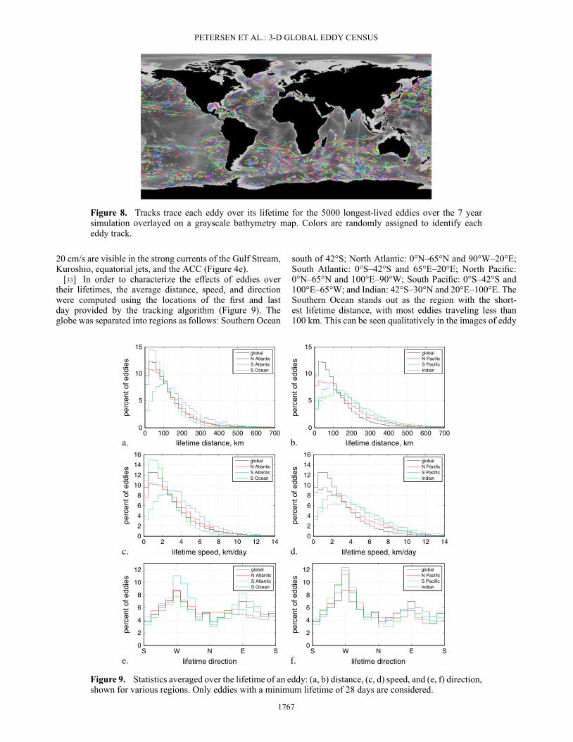
[30] Figure 7a shows a histogram of lifetimes for alleddies identified over the 7 year period. As noted above,75% of eddies identified in daily averages have lifetimes ofless than 28 days and were discarded from the analysis sincesuch short-lived eddies are typically not coherent struc-tures involved in nonlocal transport. The longest-lived eddyexisted for a duration of 1143 days, nearly half the span ofthe full data set. This eddy remains nearly still and isolatedin the Gulf of St. Lawrence (green track in Figure 8) with amean thickness of 419 m and mean diameter of 69 km. Othereddies with lifetimes greater than 550 days include three offthe coast of Chile, two in the ACC, and one in the northwestPacific.

[31] An image of the 5000 longest-lived eddies (Figure 8)shows an abundance of eddies in the ACC; these tracks

1765


a.60 40 20 0 20 40 60 80

102

103

104

105

eddies per year per 1 latitude bin

latitude

R2, life>4 wksR2, all eddiesOW, all eddies

b.60 40 20 0 20 40 60 80

200

400

600

800

1000

1200

1400

1600

thickness, m

latitude

R2, life>4 wksR2, all eddiesOW, all eddies

c.60 40 20 0 20 40 60 80

0

20

40

60

80

100

120

140diameter, km

latitude

0

40

80

120

160

200

240

280R2, life>16 wksR2, life>4 wksR2, all eddiesOW, all eddies2*Rossby Radobs (right axis)

o

Figure 6. Eddy statistics collected over a 7 year ocean simulation in 1° latitude bins: (a) daily eddycount, (b) thickness, and (c) diameter, showing the Okubo-Weiss method (blue), the R2 method (red), andthe R2 method with a minimum lifetime of 4 weeks (black) and 16 weeks (green, in Figure 6c only). Theblack dashed line in Figure 6c is 2 times the first baroclinic Rossby Radius computed using the time-averaged model density field employing the method described in section 2a of Smith et al. [2000]. Notethat this curve is almost identical to that produced from the model’s data-derived initial condition. Thepurple line in Figure 6c shows the zonally averaged speed-based radius scale from Chelton et al. [2011](note that scale is on the right axis). The R2 method is more selective than Okubo-Weiss alone, and thelifetime filter further reduces the number, particularly near the equator. Eddies rejected by the R2 methodtend to be small and thin, so that the average eddy diameter and thickness increase. Eddy numbers arecounted from each daily entry of the census data.

appear relatively short and chaotic and propagate in alldirections. In contrast, the midlatitude eddy tracks aresmoother, longer, and predominantly westward. Severaltracks have a looping behavior, such as two brown tracks inthe mid-North Atlantic. The tracked Agulhas Rings are par-ticularly long and stable and are visible all the way to SouthAmerica. Because this eddy tracking routine requires simi-lar radii to match from frame to frame, an event that changes

eddy characteristics, like merger or shearing in a jet, willsometimes split what appears to be a single track.

[32] The tracking algorithm measures the speed of eddypropagation by computing the distance traveled from 1 dayto the next (Figure 7b). The distribution follows a logarith-mic dropoff, with 72% of eddies slower than 10 cm/s and93% slower than 20 cm/s. This range is similar to observa-tions [Chelton et al., 2011, Figure 22]. Speeds higher than

a.0 100 200 300 400 500 600 700 800 900 100011001200

1

10

100

103

104

105

10

100

103

104

105

lifetime, days b.0 20 40 60 80 100

speed, cm/s

106

Figure 7. Distribution of eddies detected by (a) lifetime and (b) propagation speed, using the R2 method.The majority of eddies are relatively slow and short-lived, but some eddies exist for more than a year.In Figure 7a, the vertical axis shows the eddy count for all 7 years, and each eddy is only counted onceover its lifetime. In Figure 7b, the vertical axis shows the number of eddies per year counted in each dailysnapshot. Eddies in Figure 7b have a minimum lifetime of 4 weeks.

1766


Figure 8. Tracks trace each eddy over its lifetime for the 5000 longest-lived eddies over the 7 yearsimulation overlayed on a grayscale bathymetry map. Colors are randomly assigned to identify eacheddy track.

20 cm/s are visible in the strong currents of the Gulf Stream,Kuroshio, equatorial jets, and the ACC (Figure 4e).

[33] In order to characterize the effects of eddies overtheir lifetimes, the average distance, speed, and directionwere computed using the locations of the first and lastday provided by the tracking algorithm (Figure 9). Theglobe was separated into regions as follows: Southern Ocean

south of 42°S; North Atlantic: 0°N–65°N and 90°W–20°E;South Atlantic: 0°S–42°S and 65°E–20°E; North Pacific:0°N–65°N and 100°E–90°W; South Pacific: 0°S–42°S and100°E–65°W; and Indian: 42°S–30°N and 20°E–100°E. TheSouthern Ocean stands out as the region with the short-est lifetime distance, with most eddies traveling less than100 km. This can be seen qualitatively in the images of eddy

a.0 100 200 300 400 500 600 700

0

5

10

15

lifetime distance, km

perc

ent o

f edd

ies

0 100 200 300 400 500 600 7000

5

10

15

lifetime distance, km

perc

ent o

f edd

ies

globalN AtlanticS AtlanticS Ocean

b.

globalN PacificS PacificIndian

c.0 2 4 6 8 10 12 14

0

2

4

6

8

10

12

14

16

lifetime speed, km/day

perc

ent o

f edd

ies

0 2 4 6 8 10 12 140

2

4

6

8

10

12

14

16

lifetime speed, km/day

perc

ent o

f edd

ies


d.


e.S W N E S

0

2

4

6

8

10

12

lifetime direction

perc

ent o

f edd

ies

S W N E S0

2

4

6

8

10

12

lifetime direction

perc

ent o

f edd

ies


f.


Figure 9. Statistics averaged over the lifetime of an eddy: (a, b) distance, (c, d) speed, and (e, f) direction,shown for various regions. Only eddies with a minimum lifetime of 28 days are considered.

1767


a.0 50 100 150 200 250 300

40

50

60

70

80

90

diameter, km

perc

ent c

yclo

nic

b.0 1000 2000 3000 4000 5000 6000

42

44

46

48

50

52

54

56

58

thickness, m

perc

ent c

yclo

nic

Figure 10. Percent of eddies that are cyclonic, binned by (a) diameter and (b) thickness. Overall, 46%of eddies are cyclonic (dashed line). A strong correlation exists between cyclonicity and eddy diameter,and there appears to be little dependance on thickness.

tracks (Figure 8) and is due to the pervasively strong flowsof the ACC. Over most of the globe, there is a strong pref-erence for westward motion over the lifetime of the eddy, asexpected from Rossby wave dynamics. The Southern Oceanpresents an exception, where the eastward background flowmay be as fast or faster than the eddy’s intrinsic propagationspeed. Outside of the Southern Ocean, eddies in the North-ern Hemisphere travel shorter distances and slower speedsthan those in the Southern Hemisphere. Figure 8 showsmore long, smooth paths between the equator and 42°S,while eddy tracks in the strong western boundary currentsof the Northern Hemisphere are short and chaotic.

4.2. Eddy Diameter[34] Figure 4b shows a global view of the effective diam-

eter of the identified eddies, defined as d = 2p

A/� , where

A is the horizontal cross-sectional area of the eddy recordedat the depth with the most negative Okubo-Weiss value.Clearly the eddy diameter is a strong function of latitude,with smaller eddies near the poles and larger ones near theequator. This is expected since the first baroclinic Rossbyradius varies strongly with latitude (as shown by the dashedline in Figure 6c), and length scales for mesoscale eddiestypically are linearly related to the Rossby radius but arelarger [Stammer, 1997].

[35] Zonal averages of eddy length scales provide anotheropportunity for quantitative comparison of the R2 methodwith Okubo-Weiss, as well as with Chelton et al. [2011](Figure 6c). The R2 method removes many of the smalland poorly formed eddies identified by the Okubo-Weissmethod, thus increasing the average diameter, especiallyafter filtering out relatively short-lived eddies. As with theeddy density, comparisons of length scale with data should

a.0 40 80 120 160 200 240 280 320 360 400

diameter, km

1

10

100

103

104

105

1

10

100

103

104

105

1

10

100

103

104

105

106

1

10

100

103

104

105

106

b.0 1000 2000 3000 4000 5000 6000

thickness, m

c.0 1000 2000 3000 4000 5000 6000

depth of top of eddy, m d.0 50 100 150 200 250

depth of top of eddy, m

Figure 11. Distribution of eddies detected by (a) diameter, (b) thickness, and (c, d) depth of the top ofthe eddy, using the R2 method and minimum lifetime of 4 weeks. The last plot (Figure 11d) shows detailof the first bar in Figure 11c. Data include the population of eddies recorded each day for 7 years, andvertical axes display the number of eddies per year. The majority of eddies are small and thin, but thereare still thousands of eddies with diameters greater than 200 km and tens of thousands with thicknesses of4000–5000 m. The great majority extend to the surface (in Figure 11c), but tens of thousands exist belowthe surface.

1768


a.

b.

Figure 12. Skeletonized view of eddies in (a) the NorthAtlantic and (b) the South Atlantic. The translucent greenplanes are at 700 m (in Figure 12a) and 500 m (inFigure 12b). These images show the depth of penetration ofthe eddies; most extend to the bottom in the Antarctic Cir-cumpolar Current region, while less than half of the GulfStream eddies penetrate deeply. Eddies with positive vortic-ity are red above the planes and yellow below; eddies withnegative vorticity are blue above the planes and cyan below.Black columns extend the subsurface eddies to the surfaceto aid visualization. Depth is exaggerated by a factor of 50.(Image from Figures 4 and 5 of Williams et al. [2011a]).

focus more on shapes than magnitudes (Chelton et al. [2011]describe four methods of computing eddy length scales intheir appendix B.3, which vary by as much as a factor of3.7 in overall scale). The Pearson correlation coefficient(computed for latitudes where observations are available(68°S to 70°N) and outside of the tropics) relating the zon-ally averaged model to data length scales (black and purplecurves in Figure 6c, respectively) is 0.94; a value of 1.0is expected if the two curves are proportional or offset.

Although the model and data agree very well, they both havea somewhat weaker dependence on latitude than the Rossbyradius. Zonal averages of eddy diameter with varying confi-dence thresholds were computed using a single year’s data(Figure 3c). The Pearson correlation coefficient increasessystematically with increasing confidence threshold: 0.901for 80%, 0.925 for 85%, 0.941 for 90%, and 0.943 for 95%.The improved fit of model data versus observation pro-vides further evidence that a 90% confidence threshold is theappropriate choice for this study.

[36] Evaluating eddy diameter by region (Figure 4b), themodel agrees well with the observations (Griffa et al. [2008,Figure 3], Chelton et al. [2007, Figure 3]) in the Gulf Streamand Kuroshio Current systems, as well as in the Mozam-bique channel, in the “Cape Cauldron” [Boebel et al., 2003]to the west of the Cape of Good Hope, and along much of theSub-Antarctic Front in the ACC. However, it appears thatthe simulations and R2 method substantially underestimatethe eddy diameter in the Agulhas Retroflection (particularlydirectly south of the African continent) and the Brazil-Malvinas Confluence. The striking maximum in the SouthAtlantic at about 20°S is due to a few large Agulhas eddiesthat have traversed the ocean quite a bit too far to the north.

4.3. Cyclonicity[37] The direction of eddy rotation, averaged by 1° bins,

is shown in Figure 4d. In the Indian ocean, a blue cyclonicband is visible between 10°S and 20°S, while a red anti-cyclonic band appears between 20°S and 30°S. This issimilar to Lagrangian drifter survey data [Griffa et al.,2008, Figure 3]. The data hint at some other coherentzonal structures, but overall spatial patterns are difficultto find, much like satellite observations [Chelton et al.,2011, Figure 4].

[38] The eddy census includes more anticyclonic eddies;46% of eddies are cyclonic overall. This behavior variessmoothly with diameter, with small (large) diameter eddiestending to be more anticyclonic (cyclonic) (Figure 10a).This behavior crosses over at 120 km in diameter, and eddieslarger than 225 km in diameter have a strong preferencefor cyclonic behavior. Cyclonicity does not appear to varywith thickness in a regular way (Figure 10b). To our knowl-edge, there are no reported observations of cyclonicity as a

a.0 20 40 60 80 100

0

0.5

1

1.5

2

2.5

3

3.5

4

percent of days subsurface over lifetime

perc

ent o

f edd

ies

0 20 40 60 80 1000

0.5

1

1.5

2

2.5

3

3.5

4

percent of days subsurface over lifetime

perc

ent o

f edd

ies

global (91%)N Atlantic (92%)S Atlantic (92%)S Ocean (88%)

b.

global (91%)N Pacific (97%)S Pacific (97%)Indian (96%)

Figure 13. Distribution showing percent of days eddies are subsurface over their lifetime for variousregions for eddies with lifetimes of at least 28 days. Here subsurface means the top surface of the detectededdy is below 100 m. Parenthesis on the legends show the value of the 0–5% bin so that the vertical scalecan show the detail of the other categories. The values in the legend show that the great majority of eddiesare subsurface for 5% of the time or less; i.e., eddies nearly always extend to the surface.

1769


a.0 50 100 150 200 25010

110

1

100

101

102

lifetime, days

perc

ent o

f edd

ies

101

100

101

perc

ent o

f edd

ies

Surface EddiesSubsurface Eddies

b.0 50 100 150

100

101

mean diameter over lifetime, km

perc

ent o

f edd

ies


c.0 1000 2000 3000 4000 5000

mean thickness over lifetime, m


Figure 14. Characteristics of surface versus subsurface eddies for eddies with lifetimes of at least28 days. Subsurface eddies are defined as those below 100 m at least 50% of their lifetime, and surfaceeddies are below 100 m 5% of their lifetime or less. Subsurface eddies have a (a) shorter lifetime and (b)smaller diameter than surface eddies. (c) Subsurface eddies have a larger percentage of eddies thicker than1500 m than surface eddies. Overall, most eddies are thin surface eddies that only extend 500–1000 mbelow the surface (Figure 14c).

function of diameter or thickness. Chelton et al. [2011]reports more cyclones than anticyclones for eddies with alifetime of less than 60 weeks, which is opposite our finding.

4.4. Origin and Termination[39] The tracking algorithm allows the identification of

origin and termination locations for each eddy. These werecollected in 1° bins to show regions of origin and termi-nation (not shown). The geographical distribution of originand termination are largely the same as each other and

diameter, km

thic

knes

s, m

0 50 100 150 200 2500

1000

2000

3000

4000

5000

6000

1

10

100

1000

10^4

10^5

Figure 15. Distribution of eddies binned by diameter ver-sus thickness using R2 method and minimum lifetime of4 weeks. Colors show a log scale of number of eddiesrecorded daily, per year. For each thickness category, themean diameter is starred; for each diameter category, meanthickness is circled. A weak correlation is seen—thickeddies tend to be larger in diameter than thin eddies.

similar to daily recorded eddy locations (Figure 4a); theseare all highest in the ACC, Gulf Stream, and KuroshioCurrent regions. Chelton et al. [2011] also find that ori-gin and termination sites are common in open-oceanregions wherever propagating eddies occur (their Figure6). This is consistent with studies that show that nearlyall of the world ocean is baroclinically unstable [Smith,2007; Stammer, 1998]. Plotting the difference betweenorigin and termination global distributions (not shown),coastal regions have a higher number of eddy genera-tion sites on eastern boundaries and more terminationson western boundaries, as one would expect when amajority of eddies are propagating westward (Figures 9eand 9f). This same pattern is evident in satellite obser-vations [Chelton et al., 2011, Figure 6]. As noted byDong et al. [2012] in their regional simulations of theSouthern California Bight, eddy creation can be stronglyinfluenced by topography, which can also be seen in thisglobal simulation.

4.5. Vertical Characteristics[40] One major advantage of using fully three-

dimensional model fields is the ability to investigate thevertical characteristics of eddies. For each eddy, the R2

method finds the highest Okubo-Weiss value where the 90%confidence threshold is maintained. The three-dimensionalsurface of this Okubo-Weiss value defines the eddy extent,so that the census database includes a minimum depth,maximum depth, and thus a thickness (difference betweenthe two) for each eddy on every day. The R2 method findsthe eddy surface by determining where the Okubo-Weissvalue no longer fits, to a particular confidence threshold,

1770


a. diameter, km

lifet

ime,

day

s

0 50 100 150 200 25010

50

100

150

200

250

1

10

100

1000

10^4

10^5

b. diameter, km

spee

d, c

m/s

0 50 100 150 200 2500

10

20

30

40

50

60

1

10

100

1000

10^4

10^5

c. thickness, m

lifet

ime,

day

s

0 1000 2000 3000 4000 5000 600010

50

100

150

200

250

1

10

100

1000

10^4

d. thickness, m

spee

d, c

m/s

0 1000 2000 3000 4000 5000 60000

10

20

30

40

50

60

1

10

100

1000

10^4

10^5

Figure 16. Distribution of eddies binned by (a, c) lifetime and (b, d) propagation speed versus (a, b)diameter and (c, d) thickness, all using R2 method and minimum lifetime of 4 weeks. For each category,an asterisk is placed at the average of the horizontal variable, and a circle at the average of the verticalvariable. White areas contain no data. Colors show a log scale of number of eddies recorded daily, peryear. These trends show that longer-lived and faster eddies tend to be larger in diameter (Figures 16a and16b), and very thin eddies are shorter-lived and faster (Figures 16c and 16d).

the linear relationship that would be expected with theinclusion of additional volume if the eddy’s vorticity wereperfectly Gaussian in its dependence on radial distancefrom the core. There will be some vortical motion beyondthe eddy’s boundary surface, but it is substantially weakerthan within the eddy.

[41] The zonally binned thickness (Figure 6b) is the great-est in the Southern Ocean, due in part to a fairly uniformlongitudinal distribution in the ACC as well as some verythick eddies to the north and west of the Weddell Sea(Figure 4c). Thick eddies (�2000 m) are also typicallyfound in the extension regions of the major western bound-ary currents as well as the North Brazil Current and the Gulfof Mexico.

[42] As is the case for the horizontal scale, the R2 methoddoes not have an explicit thickness criteria, but thin eddiesare more strongly removed than with Okubo-Weiss alonebecause most poorly formed eddies are also thin. The R2

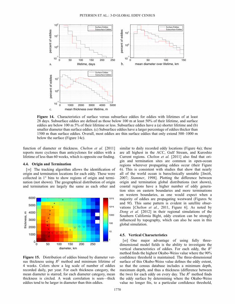
method approximately doubles the globally averaged thick-ness, compared to Okubo-Weiss, and restricting to eddieswith a minimum lifetime of 4 weeks further removes thineddies (Figure 6b).

[43] Overall, the majority of eddies are thin (Figure 11b).Still, there is a significant population of thick eddies sincethe distribution shows that 40%, 16%, and 7.7% are at least1000 m, 2000 m, and 3000 m thick, respectively. In orderto provide a qualitative image of vertical eddy extent, askeletonized view is provided in Figure 12, showing thatsome eddies extend to the full column depth in the GulfStream, while most eddies extend to the bottom in theSouthern Ocean.

[44] In addition to thickness, we can also locate theextents of eddies within the water column. The great major-

ity of eddies observed in the daily data extend all the way tothe surface (Figures 11c and 11d), with 97% expressed in themodel’s 10 m-thick uppermost threshold for eddies trackedfor at least 4 weeks and 89% with no lifetime restriction.This does not necessarily imply that the remaining eddieswould be missed in observational studies of SSH using satel-lite altimetry. Not all eddies that extend to the surface havea clear SSH signature, while some eddies that do not reachthe surface can be detected in the SSH. To quantify thepercentage of eddies that are missed would require corre-lating these results with an SSH-based detection algorithm,such as Chelton et al. [2011], which is beyond the scope ofthis paper.

[45] The tracking program allows us to quantify verticalcharacteristics over the lifetime of each eddy. To this end, wedefine “subsurface” to mean that the top of the eddy bound-ary surface is below 100 m. Figure 13 shows the percentageof days that the eddy is subsurface over its lifetime. Thegreat majority of eddies extend above 100 m at least 95% ofthe time (91% globally). One might expect that subsurfaceeddies remain so for the duration of their lifetime. However,that is not the case. Eddies tracked over their lifetime that aresubsurface some days extend to the surface on other days.Figure 13 shows that many eddies are subsurface 5–20% ofthe time, and very few are subsurface all the time.

[46] Going one step further, what are the characteristicsof subsurface eddies that will largely be missed by satelliteobservations? For this purpose, we define subsurface eddiesas those below 100 m at least 50% of their lifetime andsurface eddies as those below 100 m for 5% of their life-time or less. Subsurface eddies have a much shorter lifespanthan surface eddies, and no subsurface eddies were foundwith lifetimes longer than 125 days, while surface eddies

1771


often live for 200–600 days (Figure 14). Subsurface eddiesare smaller than surface eddies, with 40% in the 30–40 kmdiameter category. The thickness distribution does not fol-low this pattern. Most subsurface eddies are 1500–3500 mthick, while more than half of surface eddies are less than1000 m thick.

4.6. Multivariate Distributions[47] Given the numerous properties that the eddy census

provides, it is now possible to look for relationships betweenthem. For example, Figure 15 shows a two-dimensional his-togram of diameter and thickness. For most of the rangeof both diameter (50–150 m) and thickness (500–4500 m),there is no clear correlation. That is, knowledge of an eddy’sdiameter yields no specific information about its thickness,and vice versa. However, the extremes in the distributiondo show that small eddies tend to be thinner than normaland very thick eddies tend to have larger diameters thannormal. Quantitatively, the Pearson correlation coefficientbetween diameter and thickness is 0.154, where 1.0 meansthe two variables are linearly dependent, and zero impliesno correlation.

[48] Based on kinematic considerations, one might expectthat larger eddies would tend to be longer lived than smallerones since they contain more mass and momentum and areless likely to be torn apart by background shear or whenpassing over deep-sea ridges. This does appear to be the casehere. A clear correlation exists between mean eddy diameterand lifetime (stars in Figure 16a), as quantified by a Pearsoncorrelation coefficient of 0.261. Similarly, fast eddies tendto be larger in diameter (stars in Figure 16b). There alsois a noticeable relationship between thickness and speed,showing a tendency for thinner eddies to move somewhatfaster. Quantitatively, however, the Pearson correlation isonly 0.017 so this may only be relevant to speeds underabout 20 cm/s.

5. Conclusions[49] Seven years of daily output from a global high-

resolution POP simulation has allowed us to locate and char-acterize 6.7 million eddies using the R2 method [Williamset al., 2011b] and a tracking algorithm. While this work ispreceded by many studies of eddies in regional ocean simu-lations such as Doglioli et al. [2007], Nencioli et al. [2010],Souza et al. [2011b], Dong et al. [2012], Doglioli et al.[2007], and Colas et al. [2011] (a few of which also evaluatethe vertical aspects of the eddy field), we believe that this isthe first systematic eddy census of a three-dimensional high-resolution global ocean simulation. Our goal in this studyis to provide statistical information on eddies throughoutthe global ocean, as done with satellite altimetry investi-gations [Chelton et al., 2007; Chelton et al., 2011], and toalso describe eddy characteristics that are hidden below thesurface. In addition, detailed quantitative information abouteddy speed and lifetime may prove useful in attempts toparameterize the nonlocal effects of eddies in simulationswhere they are not explicitly represented.

[50] A significant number of eddies penetrate deep intothe ocean: a third of the eddies in this simulation are at least1000 m tall. Of eddies with a minimum 4 weeks lifetime,the majority (97%) extend all of the way to the surface.

Although not all of these surface-expressed eddies locatedby the R2 method are clearly reflected in the surface height,it is very likely that satellite altimetry-based assessmentsof eddy size, spatial distribution, and lifetime are reason-ably comprehensive as estimates of eddy characteristics.The remaining eddies that do not reach the surface are dis-tributed over the full depth of the ocean, with thousandsdeeper than 3000 m. Larger-diameter eddies are likely tobe thicker, longer lived, and faster than smaller-diametereddies. Correlations between thickness and lifetime or thick-ness and speed are weak, except that very thin eddies arefast and shorter lived.

[51] Any eddy census method is dependent on the eddydetection method and the parameters chosen within thatmethod. Because the R2 method is relatively new, weinclude a traditional Okubo-Weiss method in some plots fordirect comparison. The R2 method judges the quality of aneddy based on the similarity of certain functional fits with anidealized Gaussian vortex. We find that R2 is more selectivethan Okubo-Weiss and preferentially removes smaller andthinner eddies. It improves global statistics, such as meandiameter versus latitude, to be more like observations andtheoretical expectations. For this study, we have primarilyused an R2 confidence threshold of 90%, which appears tomostly select well-formed, coherent, and long-lived eddies.Absolute numbers of eddies counted are sensitive to choicesof methods and parameters used for detection, so we haveincluded distributions and percentages throughout the paper.Choices of model settings, such as diffusion coefficients andadvection schemes, can also affect the number and charac-teristics of simulated eddies, but quantifying sensitivity tothese factors is prohibitively expensive for a global eddy-ing model. In addition, experience has shown that there isa relatively narrow range of parameter space that providessmooth solutions and yet allows for strongly developedmesoscale variability that compares well with observations[Bryan et al., 2007]. Thus, it is unlikely that acceptable vari-ations in the model configuration would result in substantialchanges to the results presented here.

[52] The first priority in an ocean modeling study is toconfirm that simulations are in reasonable agreement withobservational data, wherever those data are available. Otherauthors have conducted comparisons of the POP oceanmodel at a resolution of one-tenth degree with observationsof volume transport, kinetic energy, and eddy kinetic energyand have found good agreement [Smith et al., 2000; Bryanet al., 2007; Maltrud and McClean, 2005]. In the eddydata presented here, a comparison of eddy count, diameter,and rotational direction was made with figures in Cheltonet al. [2011] and Griffa et al. [2008]. General trends, suchas increasing diameter towards the equator, are similar toobserved, but geographical distributions of eddy character-istics did not match in some cases. This was complicatedby the fact that satellite observations [Chelton et al., 2011]and drifter trajectories [Griffa et al., 2008] were not alwaysin agreement.

[53] Beyond surface studies, is there a way to confirmthe deeper data? Here we turn to Thoppil et al. [2011],who found that a simulation using the Hybrid CoordinateOcean Model (HYCOM) at 1/12.5° resolution is defi-cient in eddy kinetic energy in both the upper and abyssaloceans (depths greater than 3000 m) by 21% and 24%,

1772


respectively, compared to surface drifting buoys and deepcurrent meters (increasing the resolution to 1/25° alleviatedthe problem). Our study used a 1/10° POP simulation, butgenerally we can expect that ocean simulations at this res-olution may be underresolved for some eddy processes andmay underrepresent eddy activity, perhaps by as much as20–25%.

[54] Even with this discrepancy, we can confidently con-clude that eddies are a common phenomenon in the deepocean, albeit in smaller numbers than thin eddies near thesurface. Observational studies of eddy transport of heat andnutrients [Roemmich and Gilson, 2001; Chaigneau et al.,2011; Doglioli et al., 2007] have been confined to the upperocean for practical reasons. The next step in the analysis ofthis simulation is to quantify the impact of discrete eddieson the transport of tracers throughout the globe. Indeed,high-resolution ocean model output provides the uniqueopportunity to compute detailed statistics where observa-tions are sparse. Our team has recently developed a methodto compute tracer fluxes through eddy boundaries [Williamset al., 2012]. In future work, we plan to seed eddies in globalsimulations with passive tracers, leading to eddy transportand containment statistics for various regions of the earth.

[55] Acknowledgments. The authors thank Milena Veneziani andWilbert Weijer for early comments on the manuscript and Neesha RegmiSchnepf for assistance with the literature search on vortex identificationmethods. We also thank Richard Strelitz and Samantha Oestricher forinsightful discussions. Dudley Chelton and Michael Schlax generouslygave us access to their altimetry-derived eddy census data. M.R.P., M.W.H.,and M.E.M. were supported by the Regional and Global Climate Mod-eling programs; S.J.W. was supported by the UV-CDAT project in theClimate and Earth System Modeling programs. Both of these are within theOffice of Biological and Environmental Research of the US Department ofEnergy’s Office of Science. We acknowledge the support of the LANL-UCDavis Materials Design Institute for S.J.W. and B.H.

ReferencesAdams, D. K., D. J. McGillicuddy, L. Zamudio, A. M. Thurnherr, X.

Liang, O. Rouxel, C. R. German, and L. S. Mullineaux (2011), Surface-generated mesoscale eddies transport deep-sea products from hydrother-mal vents, Science, 332, 580–583.

Adcroft, A., C. Hill, and J. Marshall (1997), Representation of topographyby shaved cells in a height coordinate ocean model, Mon. Weather Rev.,125, 2293.

Benitez-Nelson, C. R., et al. (2007), Mesoscale Eddies drive increasedsilica export in the subtropical Pacific ocean, Science, 316, 1017–1021.

Boebel, O., J. Lutjeharms, C. Schmid, W. Zenk, T. Rossby, and C. Barron(2003), The Cape Cauldron: A regime of turbulent inter-ocean exchange,Deep-Sea Res. Pt. II, 50, 57–86.

Bryan, F. O., M. W. Hecht, and R. D. Smith (2007), Resolution convergenceand sensitivity studies with North Atlantic circulation models. Part I: TheWestern Boundary Current system, Ocean Model., 16, 141–159.

Chaigneau, A., and O. Pizarro (2005), Eddy characteristics in theeastern South Pacific, J. Geophys. Res.-Oceans, 110, 6005, doi:10.1029/2004JC002815.

Chaigneau, A., M. Le Texier, G. Eldin, C. Grados, and O. Pizarro (2011),Vertical structure of mesoscale eddies in the eastern South Pacific Ocean:A composite analysis from altimetry and Argo profiling floats , J.Geophys. Res.-Oceans, 116, 11,025, doi:10.1029/2011JC007134.

Chelton, D. B., M. G. Schlax, R. M. Samelson, and R. A. de Szoeke (2007),Global observations of large oceanic eddies, Geophys. Res. Lett., 34, 5,doi:10.1029/2007GL030812.

Chelton, D. B., M. G. Schlax, and R. M. Samelson (2011), Global observa-tions of nonlinear mesoscale eddies, Prog. Oceanogr., 91, 167–216.

Colas, F., J. C. McWilliams, X. Capet, and J. Kurian (2011), Heat balanceand eddies in the Peru-Chile current system, Clim. Dynam., 39(1-2), 582.

Dewar, W. K., and P. D. Killworth (1995), On the stability of oceanic rings,J. Phys. Oceanogr., 25, 1467–1487.

Doglioli, A. M., B. Blanke, S. Speich, and G. Lapeyre (2007), Trackingcoherent structures in a regional ocean model with wavelet analysis:Application to Cape Basin eddies, J. Geophys. Res.-Oceans, 112, 5043,doi:10.1029/2006JC003952.

Dong, C., X. Lin, Y. Liu, F. Nencioli, Y. Chao, Y. Guan, D. Chen, T. Dickey,and J. C. McWilliams (2012), Three-dimensional oceanic eddy analysisin the Southern California Bight from a numerical product, J. Geophys.Res.-Oceans, 117(C7), 2156–2202, doi:10.1029/2011JC007354.

Dukowicz, J. K., and R. D. Smith (1994), Implicit free-surface method forthe Bryan-Cox-Semtner ocean model, J. Geophys. Res., 99, 7991–8014.

Everett, J. D., M. E. Baird, and I. M. Suthers (2011), Three-dimensionalstructure of a swarm of the salp Thalia democratica within a cold-core eddy off southeast Australia , J. Geophys. Res.-Oceans, 116,12,046.X, doi:10.1029/2011JC007310.

Falkowski, P. G., D. Ziemann, Z. Kolber, and P. K. Bienfang (1991), Roleof eddy pumping in enhancing primary production in the ocean, Nature,352, 55–58.

Fang, F., and R. Morrow (2003), Evolution, movement and decay of warm-core Leeuwin Current eddies, Deep-Sea Res. Pt. II, 50, 2245–2261.

Godø, O. R., A. Samuelsen, G. J. Macaulay, R. Patel, S. S. Hjøllo, J. Horne,S. Kaartvedt, and J. A. Johannessen (2012), Mesoscale eddies are oasesfor higher trophic marine life, PLoS ONE, 7, e30,161.

Griffa, A., R. Lumpkin, and M. Veneziani (2008), Cyclonic and anticy-clonic motion in the upper ocean , Geophys. Res. Lett., 35, 1608, doi:10.1029/2007GL032100.

Griffies, S.M., et al. (2009), Coordinated Ocean-Ice Reference Experiments(COREs), Ocean Model., 26, 1–46.

Henson, S. A., and A. C. Thomas (2008), A census of oceanic anticycloniceddies in the Gulf of Alaska, Deep-Sea Res. Pt. I, 55, 163–176.

IPCC (2007), Climate Change 2007: The Physical Science Basis. Con-tribution of Working Group I to the Fourth Assessment Report ofthe Intergovernmental Panel on Climate Change, 996 pp., CambridgeUniversity Press, Cambridge U. K.

Isern-Fontanet, J., E. Garca-Ladona, and J. Font (2003), Identification ofmarine eddies from altimetric maps, J. Atmos. Ocean. Tech., 20, 772.

Isern-Fontanet, J., E. Garca-Ladona, J. Font, and A. Garca-Olivares(2006), Non-Gaussian velocity probability density functions: An alti-metric perspective of the mediterranean sea, J. Phys. Oceanogr., 36,2153–2164.

Kundu, P. K., I. M. Cohen, and D. R. Dowling (2012), Fluid Mechanics,5th ed., 920 pp., Academic Press, New York, N. Y.

Large, W. G., J. C. McWilliams, and S. C. Doney (1994), Oceanic ver-tical mixing: A review and a model with a nonlocal boundary layerparameterization, Rev. Geophys., 32, 363–404.

de Leeuw, W. C., and F. H. Post (1994), A statistical view on vector fields,in Visualization in Scientific Computing, edited by M. Göbel, H. Müller,and B. Urban, pp. 53–62, Springer-Verlag Wein.

Lilly, J. M., and P. B. Rhines (2002), Coherent eddies in the labrador seaobserved from a mooring, J. Phys. Oceanogr., 32, 585–598.

Mahadevan, A., E. D’Asaro, C. Lee, and M. J. Perry (2012), Eddy-driven stratification initiates north atlantic spring phytoplankton blooms,Science, 337, 54–58.

Maltrud, M., F. Bryan, and S. Peacock (2010), Boundary impulse responsefunctions in a century-long eddying global ocean simulation, Environ.Fluid. Mech., 10, 275–295, doi:10.1007/s10652-009-9154-3.

Maltrud, M. E., and J. L. McClean (2005), An eddy resolving global 1/10°ocean simulation, Ocean Model., 8, 31–54.

Maslowski, W., J. L. C. Kinney, D. C. Marble, and J. Jakacki (2008),Towards eddy-resolving models of the Arctic ocean, in Ocean Mod-eling in an Eddying Regime, edited by M. Hecht, and H. Hasumi,pp. 241–264, no. 177 in Geophysical Monograph Series, AmericanGeophysical Union, Washington, D.C.

Meehl, G. A., et al. (2006), Climate change projections for the twenty-firstcentury and climate change commitment in the CCSM3, J. Climate, 19,2597–2616.

Nencioli, F., C. Dong, T. Dickey, L. Washburn, and J. C. McWilliams(2010), A vector geometry-based eddy detection algorithm and its appli-cation to a high-resolution numerical model product and high-frequencyradar surface velocities in the Southern California Bight, J. Atmos.Ocean. Tech., 27, 564–579.

Nishino, S., M. Itoh, Y. Kawaguchi, T. Kikuchi, and M. Aoyama (2011),Impact of an unusually large warm-core eddy on distributions ofnutrients and phytoplankton in the southwestern Canada Basin duringlate summer/early fall 2010 , Geophys. Res. Lett., 38 (16), 602, doi:10.1029/2011GL047885.

Paillet, J., C. Le B., X. Carton, Y. Morel, and A. Serpette (2002), Dynamicsand evolution of a Northern Meddy, J. Phys. Oceanogr., 32, 55–79.

Petersen, M. R., K. Julien, and J. B. Weiss (2006), Vortex cores, strain cells,and filaments in quasigeostrophic turbulence, Phys. Fluids, 18, 026601,11 pp., doi:10.1063/1.2166452.

1773


Prater, M. D. (2002), Eddies in the Labrador Sea as observed by profilingRAFOS floats and remote sensing, J. Phys. Oceanogr., 32, 411–427.

Riser, S. C., W. B. Owens, H. T. Rossby, and C. C. Ebbesmeyer (1986),The structure, dynamics, and origin of a small-scale lens of water in theWestern North Atlantic thermocline, J. Phys. Oceanogr., 16, 572–590.

Roemmich, D., and J. Gilson (2001), Eddy transport of heat and thermo-cline waters in the North Pacific: A key to interannual/decadal climatevariability? J. Phys. Oceanogr., 31, 675–688.

Sadarjoen, I. A., and F. H. Post (2000), Detection, quantification, andtracking of vortices using streamline geometry, Comput. Graph., 24,333–341.

Shoosmith, D. R., P. L. Richardson, A. S. Bower, and H. T. Rossby (2005),Discrete eddies in the northern North Atlantic as observed by loopingRAFOS floats, Deep-Sea Res. Pt. II, 52, 627–650.

Smith, K. S (2007), The geography of linear baroclinic instability in Earth’soceans, J. Mar. Res., 65, 655–683.

Smith, R. D., J. K. Dukowicz, and R. C. Malone (1992), Parallel oceangeneral circulation modeling, Physica D, 60, 38–61.

Smith, R. D., M. E. Maltrud, F. O. Bryan, and M. W. Hecht (2000), Numer-ical simulation of the North Atlantic Ocean at 1/10°, J. Phys. Oceanogr.,30, 1532–1561.

Souza, J. M. A. C., C. de Boyer Montégut, C. Cabanes, and P. Klein(2011a), Estimation of the Agulhas ring impacts on meridional heatfluxes and transport using ARGO floats and satellite data, Geophys. Res.Lett., 38(21), 602, doi:10.1029/2011GL049359.

Souza, J. M. A. C., C. de Boyer Montégut, and P. Y. Le Traon (2011b),Comparison between three implementations of automatic identificationalgorithms for the quantification and characterization of mesoscale eddiesin the South Atlantic Ocean, Ocean Sci., 7, 317–334.

Stammer, D. (1997), Global characteristics of ocean variability estimatedfrom regional TOPEX/POSEIDON Altimeter measurements, J. Phys.Oceanogr., 27, 1743–1769.

Stammer, D (1998), On eddy characteristics, eddy transports, and meanflow properties, J. Phys. Oceanogr., 28, 727–739.

Thoppil, P. G., J. G. Richman, and P. J. Hogan (2011), Energetics of a globalocean circulation model compared to observations, Geophys. Res. Lett.,38(15), 607, doi:10.1029/2011GL048347.

Timmermans, M.-L., J. Toole, A. Proshutinsky, R. Krishfield, andA. Plueddemann, (2008), Eddies in the Canada basin, arctic ocean,observed from ice-tethered profilers, J. Phys. Oceanogr., 38, 133.

Williams, S., M. Hecht, M. Petersen, R. Strelitz, M. Maltrud, J. Ahrens,M. Hlawitschka, and B. Hamann (2011a), Visualization and analysisof eddies in a global ocean simulation, Comput. Graph. Forum, 30,991–1000.

Williams, S., M. Petersen, P.-T. Bremer, M. Hecht, V. Pascucci, J. Ahrens,M. Hlawitschka, and B. Hamann (2011b), Adaptive extraction andquantification of geophysical vortices, IEEE T. Vis. Comput. Gr., 17,2088–2095.

Williams, S., M. Petersen, M. Hecht, M. Maltrud, J. Patchett, J. Ahrens,and B. Hamann (2012), Interface exchange as an indicator for eddy heattransport, Comput. Graph. Forum, 31, 1125–1134.

Williams, S. J. (2012), Identification and quantification of mesoscale eddiesin a global ocean simulation, Ph.D. thesis, University of California,Davis.

Xiu, P., F. Chai, L. Shi, H. Xue, and Y. Chao (2010), A census of eddyactivities in the South China Sea during 1993-2007, J. Geophys. Res.,115, 564–579, doi:10.1029/2009JC005657.

1774

a threedimensional eddy census of a highresolution...

Documents