a top-down approach of surface carbonyl sulfide exchange by a

Atmos. Chem. Phys., 16, 14909–14923, 2016www.atmos-chem-phys.net/16/14909/2016/doi:10.5194/acp-16-14909-2016© Author(s) 2016. CC Attribution 3.0 License.

A top-down approach of surface carbonyl sulfide exchange by aMediterranean oak forest ecosystem in southern FranceSauveur Belviso1, Ilja Marco Reiter2,3, Benjamin Loubet4, Valérie Gros1, Juliette Lathière1, David Montagne4,Marc Delmotte1, Michel Ramonet1, Cerise Kalogridis1, Benjamin Lebegue1, Nicolas Bonnaire1, Victor Kazan1,Thierry Gauquelin5, Catherine Fernandez5, and Bernard Genty3

1Laboratoire des Sciences du Climat et de l’Environnement, LSCE/IPSL, CEA-CNRS-UVSQ, Université Paris-Saclay,91191 Gif-sur-Yvette, France2CNRS, FR 3098 ECCOREV, Europôle de l’Arbois, 13545 Aix-en-Provence, France3CEA, CNRS, Aix-Marseille University, UMR 7265 Biologie Végétale et Microbiologie Environnementales,13115 Saint Paul-lez-Durance, France4AgroParisTech, INRA, Université Paris-Saclay, UMR 1402 Ecosys, 78 850 Thiverval-Grignon, France5Aix Marseille Univ, Avignon Université, CNRS, IRD, IMBE Institut Méditerranéen de Biodiversité etd’Ecologie marine et continentale, Marseille, France

Correspondence to: Sauveur Belviso ([email protected])

Received: 16 June 2016 – Published in Atmos. Chem. Phys. Discuss.: 5 July 2016Revised: 26 October 2016 – Accepted: 13 November 2016 – Published: 2 December 2016

Abstract. The role that soil, foliage, and atmospheric dy-namics have on surface carbonyl sulfide (OCS) exchange in aMediterranean forest ecosystem in southern France (the OakObservatory at the Observatoire de Haute Provence, O3HP)was investigated in June of 2012 and 2013 with essentiallya top-down approach. Atmospheric data suggest that the siteis appropriate for estimating gross primary production (GPP)directly from eddy covariance measurements of OCS fluxes,but it is less adequate for scaling net ecosystem exchange(NEE) to GPP from observations of vertical gradients of OCSrelative to CO2 during the daytime. Firstly, OCS and carbondioxide (CO2) diurnal variations and vertical gradients showno net exchange of OCS at night when the carbon fluxesare dominated by ecosystem respiration. This contrasts withother oak woodland ecosystems of a Mediterranean climate,where nocturnal uptake of OCS by soil and/or vegetation hasbeen observed. Since temperature, water, and organic carboncontent of soil at the O3HP should favor the uptake of OCS,the lack of nocturnal net uptake would indicate that its grossconsumption in soil is compensated for by emission pro-cesses that remain to be characterized. Secondly, the uptakeof OCS during the photosynthetic period was characterizedin two different ways. We measured ozone (O3) depositionvelocities and estimated the partitioning of O3 deposition be-

tween stomatal and non-stomatal pathways before the startof a joint survey of OCS and O3 surface concentrations. Weobserved an increasing trend in the relative importance of thestomatal pathway during the morning hours and synchronoussteep drops of mixing ratios of OCS (amplitude in the rangeof 60–100 ppt) and O3 (amplitude in the range of 15–30 ppb)after sunrise and before the break up of the nocturnal bound-ary layer. The uptake of OCS by plants was also character-ized from vertical profiles. However, the time window forcalculation of the ecosystem relative uptake (ERU) of OCS,which is a useful tool for partitioning measured NEE, waslimited in June 2012 to a few hours after midday. This wasdue to the disruption of the vertical distribution of OCS byentrainment of OCS rich tropospheric air in the morning andbecause the vertical gradient of CO2 reverses when it is stilllight. Moreover, polluted air masses (up to 700 ppt of OCS)produced dramatic variation in atmospheric OCS /CO2 ra-tios during the daytime in June 2013, further reducing thetime window for ERU calculation.

Published by Copernicus Publications on behalf of the European Geosciences Union.

14910 S. Belviso et al.: A top-down approach of surface carbonyl sulfide exchange

1 Introduction

Terrestrial ecosystems modulate the water balance over landand fix carbon dioxide (CO2) from the atmosphere in theform of carbon-rich materials. Experimental and modelingstudies have shown that changes in atmospheric CO2 con-centration and changes in climate, induced by increasing an-thropogenic emissions of greenhouse gases, impact the fix-ation of atmospheric CO2 by plants (gross primary produc-tion, GPP) and the release of CO2 by terrestrial ecosystems(respiration, Reco) as modulated by temperature and wateravailability and the effects of fertilization (e.g., Arora andBoer, 2014). Large uncertainties in the determination in GPPand Reco fluxes at the continental scale and in the magnitudeof effects induced by climate and fertilization remain. Fur-thermore, experimental and modeling studies should help tobetter constrain those fluxes.

In the late 1980s, vegetation was proposed to be the miss-ing sink in the global cycle of atmospheric carbonyl sulfide(OCS; Brown and Bell, 1986; Goldan et al., 1988) and thefirst evidence from field observations of the uptake of OCSnear the ground was provided by Mihalopoulos et al. (1989).Today, the mechanistic link between leaf CO2 and OCS ex-change is well understood (Stimler et al., 2010; Seibt et al.,2010; Wohlfahrt et al., 2012) and the scientific communityhas reached consensus on the potential of atmospheric OCSmeasurements to provide independent constraints on GPPat canopy (Blonquist et al., 2011; Asaf et al., 2013), re-gional (Campbell et al., 2008), and global (Montzka et al.,2007; Berry et al., 2013; Launois et al., 2015) scales. How-ever, recent studies also demonstrated limitations to the useof OCS as a GPP proxy at canopy and ecosystem scalesbecause (1) consumption and/or production of OCS occurin soil and litter (Van Diest and Kesselmeier, 2008; Sun etal., 2015; Ogée et al., 2016; Whelan et al., 2016 and ref-erences therein), (2) in agricultural fields and midlatitudeforests OCS can also be taken up by plants at night (Maseyket al., 2014; White et al., 2010; Commane et al., 2015), and(3) the leaf relative uptake of OCS and of CO2 (LRU), whichis of central importance in the calculation of GPP from eddycovariance measurements of OCS exchange (LOCS) follow-ing Eq. (1), exhibit daily and seasonal variations of variableamplitudes (Berkelhammer et al., 2014; Maseyk et al., 2014;Commane et al., 2015).

GPP=LOCS

LRU×[CO2]

[OCS](1)

The character L in LOCS stands for leaf because OCS ex-change equals LOCS when other ecosystem fluxes are negli-gible. To address the diel LRU variations and the role of soiland litter for canopy scale analysis, some research groups arenow combining canopy flux, leaf, and soil chamber measure-ments in the field (L. Kooijmans personal communication,September 2016).

Equation (1) can also be used for regional scale analysis(Campbell et al., 2008). At this scale, LRU also varies as afunction of plant type (i.e., C3 vs. C4 plants, Stimler et al.,2011). However, Hilton et al. (2015) demonstrated that theeffect of LRU variability was less significant at regional thanat canopy scale because the regional spatial uncertainty inGPP is much larger than the LRU uncertainty.

The use of leaf and soil chambers offers a means of in-vestigating in laboratory and field conditions the ability ofplants and soils to degrade ambient OCS (e.g., Stimler etal., 2010; Sun et al., 2015). Approaches that avoid manipula-tion of biological material, such as the eddy flux, gradient, orradon-tracer methods (e.g., Maseyk et al., 2014; Commaneet al., 2015; Belviso et al., 2013), can document over shortand long time spans the direction and the magnitude of sur-face OCS exchange at the ecosystem level. At continental orglobal scales, biosphere–atmosphere fluxes can be assessedfrom dynamic global vegetation models, and all flux com-ponents can be optimized using satellite or global networkdata (e.g., Berry et al., 2013; Launois et al., 2015; Kuai et al.,2015). The global network NOAA ESRL for measurementsof greenhouse gases in the atmosphere has been monitoringOCS mixing ratios on a weekly basis since 2000 (Montzkaet al., 2007). It is in this framework that the major role ofvegetation in the global budget of OCS was again empha-sized. A second network (AGAGE) exists where air samplesare analyzed every 60 min, but OCS data are not yet avail-able for public access. Other sites have recently been instru-mented for long-term monitoring of atmospheric OCS con-centrations and/or fluxes. They include a mixed temperateforest in North America (Harvard forest; Commane et al.,2015), a boreal pine forest in southern Finland (Hyytiälä;A. Praplan, personal communication, 2015), and a station lo-cated on the northern coast of the Netherlands (Lutjewad;H. Chen, personal communication, 2014; Kooijmans et al.,2016). Although rural and suburban areas have also been in-strumented for shorter periods (Berkelhammer et al., 2014;Belviso et al., 2013 and references therein), many biomes re-main unexplored. In summer 2012 and 2013, we used thefacilities of the experimental field site Oak Observatory atthe Observatory of the Haute Provence (O3HP), Saint Michell’Observatoire, France, to study the biosphere–atmosphereexchanges of three atmospheric compounds (OCS, CO2, andozone, O3), which share stomatal uptake as a common path-way. O3HP is a Mediterranean forest ecosystem with lowcanopy height dominated by deciduous downy oak, Quer-cus pubescens, and Montpellier Maple, Acer monspessu-lanum. Often occurring in the transition of climate zonesfrom Mediterranean to sub-Mediterranean, and thus poten-tially rather sensitive and responsive to climate change, Q.pubescens is an interesting model to monitor changes affect-ing the Mediterranean forest ecosystems.

Our top-down approach, similar to the approach by Blon-quist et al. (2011), aims to determine the role of soil, fo-liage, atmospheric dynamics, and air pollution in surface

Atmos. Chem. Phys., 16, 14909–14923, 2016 www.atmos-chem-phys.net/16/14909/2016/

S. Belviso et al.: A top-down approach of surface carbonyl sulfide exchange 14911

OCS exchange at the O3HP, finding consistencies and dif-ferences with other oak woodland ecosystems characterizedby a Mediterranean climate, and assessing the desirabilityof using OCS to partition O3 deposition between stomataland non-stomatal pathways. Since direct LRU and OCS fluxmeasurements were not performed during the campaigns,we used the ecosystem relative uptake (ERU) approach ofCampbell et al. (2008) to provide a rough estimation of LRUvariations using the following equation:

LRU= [ERU]×[NEE][GPP]

, (2)

where ERU is the relative gradient of OCS (m−1) dividedby the relative gradient of CO2 (m−1) and NEE is the netecosystem exchange of CO2 from eddy covariance measure-ments carried out at the site.

2 Material and methods

2.1 Description of the site and of air circulation

The two campaigns took place in June of 2012 and 2013.Both were of short duration (i.e., about 2 weeks). A descrip-tion of the O3HP site is available in Kalogridis et al. (2014)and Santonja et al. (2015). In short, the site (43.93◦ N,5.71◦ E) is located on the premises of Observatoire de HauteProvence, about 60 km north of Marseille, France, at an el-evation of 680 m above mean sea level. It is implementedin a forest area that has remained untouched since at least1945. The climate is sub-Mediterranean with dry, warm-to-hot summers.

The O3HP observatory is characterized by a highly hetero-geneous karstic limestone with soil pockets developing be-tween compact and hard limestone bedrock. The soils, whichnever exceed 1 m depth, range from shallow calcaric Lep-tosol to deeper calcaric Cambisols (IUSS Working GroupWRB, 2014). The litter overlying the A horizons (O hori-zons) is 1–7 cm strong. The A horizons of 2–10 cm depthare clayey, calcareous, and show high organic carbon con-tent (Table 1). These horizons have a strong, crumbly-to-finesubangular blocky structure likely due to high earthwormburrowing activity and numerous fine roots. The humus isan “active oligomull or dysmull type” (Brêthes et al., 1995).The A/C horizon consists of thin layers of a clayey and fineblocky soil material between limestone rocks of a decametricsize. Roots are observed inside the thin soil layers.

Downy oak (Quercus pubescens) and Montpellier maple(Acer monspessulanum L.) represent 75 and 25 %, respec-tively, of the foliar biomass of the dominant tree species(Kalogridis et al., 2014). The coppice, typically constitutedby multiple stems sprouting from the same rooting sys-tem, is about 70 years old. Mean tree height is 5 m, andmean diameter at breast height is 10 cm, ranging from 0.9to 18.6 cm. European smoke bush (Cotinus coggygria Scop.)

and many thermophilic and xerophilic herbaceous and grassspecies compose the understorey vegetation (Kalogridis etal., 2014). A network of soil sensors beneath and above thecanopy continuously record environmental parameters, in-cluding global radiation, air and soil temperature profiles,air and soil moisture, wind speed, and rainfall, which aremade accessible through the COOPERATE database (http://cooperate.obs-hp.fr/db).

Our understanding of the atmospheric dynamics over theO3HP sampling site does not rely solely on meteorologicalparameters recorded at ground level by basic weather sta-tions. The transport and dispersion of air pollutants in thesoutheastern part of France was extensively investigated dur-ing the “Expérience sur Site pour Contraindre les Modèles dePollution atmosphérique et de Transport d’Emissions” (ES-COMPTE) experiment, which took place in June–July 2001(Cros et al., 2004; Kalthoff et al., 2005). As shown by theseauthors for June 2001 and in Fig. S1 in the Supplement forJune of 2012, 2013, and 2015, the sea breeze is a generalcharacteristic of the atmospheric dynamics at the site in June.It flows from the W-SW in the afternoon and carries with itthe photosmog of the city of Marseille. During the night andearly morning hours the wind is oriented from other direc-tions with a strong N-NE component (Fig. S1). However, onefundamental aspect of air circulation over the area is the ex-istence of a nocturnal jet flowing at 800–1000 m of altitude,also with a strong N-NE component, observed in the sodar(vertical wind profiler) measurements performed by Kalthoffet al. (2005). This is of crucial importance for the interpreta-tion of our results.

2.2 Air sampling and analytical methods

2.2.1 Momentum, energy, and CO2 and isoprene fluxes

In June 2012, momentum, energy, and CO2 fluxes were mea-sured at the O3HP site by the eddy covariance method usinga Gill-R3-HS ultrasonic anemometer placed above the for-est on a 10 m mast and a close-path infrared CO2 and H2Ogas analyzer (IRGA, Licor 7000) placed in a truck at about35 m from the base of the mast (Kalogridis et al., 2014).Air was drawn from an inlet located ∼ 20 cm away fromthe anemometer, with a 45 m long heated PFA Teflon tub-ing (1/2′′ OD, 3/8′′ ID, heated∼ 1 ◦C above ambient air tem-perature) at a flow rate of ∼ 64 L min−1 in order to maintaina turbulent flow. Air was then subsampled in a tube (1/4′′

OD, 1/8′′ ID) to the close-path IRGA. Data were sampled at20 Hz. Essentially, the turbulent flux of CO2 was estimated asthe covariancew′c′ of the vertical component of the wind ve-locity (w) and the dry mole fraction of CO2 (c), multiplied bythe dry air molar volume. Here the primes denote a deviationfrom the mean. The friction velocity u∗ =−

√w′u′, where

u is the along-wind air velocity component. High-frequencyloss corrections were estimated with the method of Ammannet al. (2006) and averaged 10 % (median). The fluxes (NEE,

www.atmos-chem-phys.net/16/14909/2016/ Atmos. Chem. Phys., 16, 14909–14923, 2016

http://cooperate.obs-hp.fr/db

http://cooperate.obs-hp.fr/db


Table 1. Soil physicochemical characteristics at O3HP.

Horizon Depth < 2 µm 2–50 µm 50–2000 µm TOC∗ N pH CaCO3(cm) (g kg−1) (g kg−1) (g kg−1) (g kg−1) (g kg−1) (g kg−1)

LeptosolA1 0–5 560 340 96 167 8.9 7.1 6A2 5–20 536 338 118 43.1 2.7 7.6 10.7A/C 20–50 515 324 133 23.3 1.7 8.0 27.2

∗ Total Organic Carbon.

GPP, and Reco) were calculated using the eddy covariancemethod as explained in Aubinet et al. (2000) and Loubet etal. (2011). In short, GPP and Reco were estimated with themethod described by Kowalski et al. (2004). Briefly, the netflux of CO2 (NEE) was modeled as the sum of the ecosystemrespiration (Reco) and the GPP (or assimilation) was mod-eled as a hyperbolic function of the incoming solar radiation(Rs).

NEE=−Reco+a1×Rsa2+Rs

=−Reco+GPP (3)

By convention here Reco and GPP are positive, and NEE iscounted positive when carbon is fixed by the canopy. The pa-rameters Reco, a1, and a2 were estimated by minimizing thedifference between the modeled and measured CO2 flux from16 May to 17 June 2012 using the nonlinear solver in Ex-cel and the objective function ln (mean square error betweenmodel and measurements). The comparison was only per-formed for well-established turbulence (u∗ > 0.1 m s−1 and|zL|< 0.2, where L is the Obukhov length) during dry peri-

ods without rain and during the daytime (Rs > 5 W m−2). TheGPP was then calculated as GPP= a1×Rs

a2+Rs for all conditions.Q. pubescens is a high-isoprene emitter and studies at

the O3HP have shown that it is the main volatile organiccompound (VOC) released by this species at the branch(Genard-Zielinski et al., 2015) and canopy scale (Kalogridiset al., 2014). Isoprene is synthesized within the leaf throughmetabolic processes and its emission in the atmosphere ismainly controlled by temperature and radiation (Laotha-wornkitkul et al., 2009 and references therein). Although itdoes not share a common source and sink with OCS, it wasused here as additional information to understand biologicalprocesses occurring at the O3HP forest.

2.2.2 Carbonyl sulfide (OCS)

At the O3HP site, in June 2012, air was drawn either froman inlet located at 10 m height ∼ 20 cm away from theanemometer or from a second inlet located at 2 m heighton the same mast with 70–80 m long Synflex tubing (3/8′′

OD) flushed permanently at a flow rate of ∼ 6 L min−1. InJune 2013, air was drawn solely from an inlet located at 2 mheight, with 20 m long Synflex tubing (3/8′′ OD). The an-alytical instruments were run in laboratory-like conditions

(air conditioning at 25 ◦C) in a small building away fromthe sampling plot. How the air was analyzed for OCS wasdescribed extensively in Belviso et al. (2013). However, themass spectrometer detector was replaced in April 2012 bya pulsed flame photometric detector (PFPD). In general, airmeasurements (500 mL STP of air trapped cryogenically at100 mL min−1 flow rate with an ENTECH preconcentrator)were carried out on an hourly basis. Peak integration wasdone using SRI’s PeakSimple Chromatography Data Sys-tem. Calibration was performed as in Belviso et al. (2013),but the primary standard, drawn with a gas-tight syringe,was injected in a line flushed with OCS-free helium (Hewas passed through an empty stainless-steel trap immersedin liquid nitrogen) connected to the preconcentrator inlet.Although the calibration gas commercialized by Air Prod-ucts has a tolerance of 2.5 %, we found an agreement bet-ter than 0.2 % between the certificate of analysis (1.013 ppmof OCS in helium) and our own measurements of that stan-dard (1.014± 0.011 ppm, n= 6) using a second calibrationgas provided by U. Seibt and K. Maseyk, who purchased itfrom Air Liquide (0.517 ppm in nitrogen). Since the PFPDresponse is quadratic, the calibration equation is obtainedby plotting the natural logarithm of the peak area againstthe natural logarithm of OCS (picolitre or pL). Mixing ra-tios are calculated by dividing pL of OCS by volumes of airdried at−25 ◦C, corrected to room temperature and pressure.Semicontinuous measurement repeatability is 1 % (1 SD,n= 38 consecutive hourly analyses of atmospheric air from acompressed cylinder (target gas) containing 573 ppt of OCS).Accuracy and long-term repeatability (LTR) were better than2.5 % as evaluated from periodic analyses of an atmosphericair standard prepared and calibrated by NOAA ESRL con-taining 448.6 ppt of OCS.

In June 2013, air was analyzed continuously for OCSusing a commercially available OCS, CO2, H2O, and COoff-axis integrated cavity output spectroscopy analyzer (LosGatos Research, Enhanced Performance Model, California,USA). In early 2013 at the O3HP, the instrument was testedfor the first time in the field. We calibrated the instrumentwith OCS measured by the GC (over a range of atmo-spheric concentrations of 439 to 699 ppt inherent to the pe-riod of interest for this study). OCS data collected with aone-half Hz frequency by the spectroscopy analyzer were



subsequently reduced to 5 min averages that correspondedto the sampling time of the GC. The OCS signal varied byless than ±2 ppt (standard error) in the 5 min time window.GC and LGR data showed a linear and strong positive cor-relation (OCSGC = 1.14OCSLGR+12.3 ppt, R2

= 0.95, n=128). Absolute readings were regularly cross-checked witha NOAA ESRL standard showing good stability throughoutthe campaign. OCSLGR data were essentially used to docu-ment OCS variations in between GC measurements, and theywere scaled to GC data using the relationship above.

2.2.3 Carbon dioxide (CO2)

At the O3HP site in June 2012, air was analyzed forCO2 from two sampling lines (10 and 2 m height), alter-nately (measurement interval duration was 30 min and datacollected during the first 10 min were discarded) using acommercially available PICARRO cavity ring-down spec-troscopy (CRDS) analyzer (Model G2401) placed next to theOCS gas chromatograph. In addition to CO2, this instrumentanalyzes CH4 and CO mixing ratios and applies correctionsfor water vapor levels. Precision and stability of the measure-ments performed with this instrument were investigated us-ing the rigorous testing procedures described by Yver Kwoket al. (2015) and reported in Table 1 of that paper (see instru-ment G2401 with serial number CFKADS2022 and ICOSID 108). For CO2, similar or better results in terms of con-tinuous measurement repeatability (CMR) and LTR were ob-tained in the field as compared to the factory or the test labo-ratory (i.e., 0.027 and 0.020 ppm), respectively (Yver Kwoket al., 2015). The CRDS analyzer was calibrated in the testlaboratory following ICOS standard procedures, once beforeshipping and right after the 1-month deployment in the field.

In June 2013, air was analyzed continuously for CO2 us-ing the LGR Enhanced Performance instrument (see above).CO2 measurements were not reported on a calibration scale.

2.2.4 Carbon monoxide (CO)

At the O3HP site in June 2012, air was analyzed for CO us-ing the PICARRO CRDS analyzer described above. Preci-sion in terms of CMR and LTR measured in the field was notas good as in the factory or the test laboratory (i.e., 6.8 and2.2 ppb, respectively) (Yver Kwok et al., 2015). Data werecalibrated as for CO2 measurements. In June 2013, air wasanalyzed continuously for CO using the LGR instrument.CO measurements were not reported on a calibration scale.CO was used as a semiquantitative tracer of combustion pro-cesses (biomass or fossil fuel burning).

2.2.5 Ozone (O3), O3 deposition velocity (VdO3) and itspartitioning

Ozone was measured at O3HP in June 2012 with an in-strument based on ultraviolet absorption (model T-400 fromAPI-Teledyne, San Diego, USA). This instrument, calibratedwith an internal ozone generator (IZS, API), is operated witha flow rate of about 700 mL min−1 and delivers data ev-ery minute. In June 2013, ozone concentrations measuredat a few hundred meters from the main O3HP site weredownloaded from the regional air quality network Air-Paca,France, (http://www.airpaca.org/). Ozone deposition velocity(VdO3) was measured at the O3HP in June 2012 with a fastO3 chemiluminescent analyzer (ATDD, NOAA, USA). Theratio method described in Muller et al. (2010) was appliedto evaluate VdO3. Detailed description of the methodology isgiven in Stella et al. (2011). The canopy conductance (gcO3)

and non-stomatal conductance for ozone (gnsO3) were esti-mated following Lamaud et al. (2009) as gcO3 = VdO3/(1−VdO3/VmaxO3), and gnsO3 = gcO3− gsO3, where the stom-atal conductance for O3 (gsO3) is equal to gsH2O×0.653,this factor being the ratio of molecular diffusivities of O3to H2O. VmaxO3 is the maximum deposition velocity forozone, which corresponds to a perfect sink of ozone atthe leaf level. This is the inverse of the sum of aerody-namic (Ra) and canopy boundary layer resistances (RblO3)

as VmaxO3 = 1/(Ra+RblO3), those being estimated as inLamaud et al. (2009), taken from Bassin et al. (2004).

2.2.6 Stomatal conductance

Canopy stomatal conductance for water vapor (gsH2O) wasestimated in 2012 from the latent (LE) and sensible (H) heatflux from the Penman–Monteith method for relative humid-ity ≤ 70 %. Under wet conditions the stomatal conductancewas estimated following Lamaud et al. (2009) based on theproportionality between the assimilation of CO2 and the con-ductance.

Leaf stomatal conductance was measured in June 2013with a porometer (AP4, Delta-T Devices, Burwell, UK).Due to the unilateral distribution of stomata (hypostomatousleaf) only the abaxial sides of the leaf were measured usingthe “slotted” configuration of the chamber. Five leaves weresampled per tree and cycle. Light was measured holding thesensor horizontally above the leaf.

3 Results

3.1 Meteorological conditions and soil climate

The cumulated precipitations before the campaigns wereabout 400 and 500 mm since the beginning of the year(Fig. 1a). As few precipitation events of small intensity tookplace during the campaigns, the volumetric soil water con-tent (measured at 5 cm depth) was in a decreasing phase from


http://www.airpaca.org/


Figure 1. Monthly variations (a) in air temperature and cumulated precipitations and (b) in soil temperature and moisture (−10 cm) at an oakforest ecosystem in southern France (O3HP). (c, d) Same as panel (b) but for June 2012 and June 2013. The yellow vertical bands correspondto the sampling periods.

about 0.3 m3 m−3 during the wet season to about 0.1 m3 m−3

during the dry season (Fig. 1b). Soil temperatures went theopposite way (Fig. 1b) and were in the range of 14–19 and14–17 ◦C during the 2012 and 2013 campaigns, respectively(Fig. 1c, d).

3.2 Diel variations in the canopy (2 m)

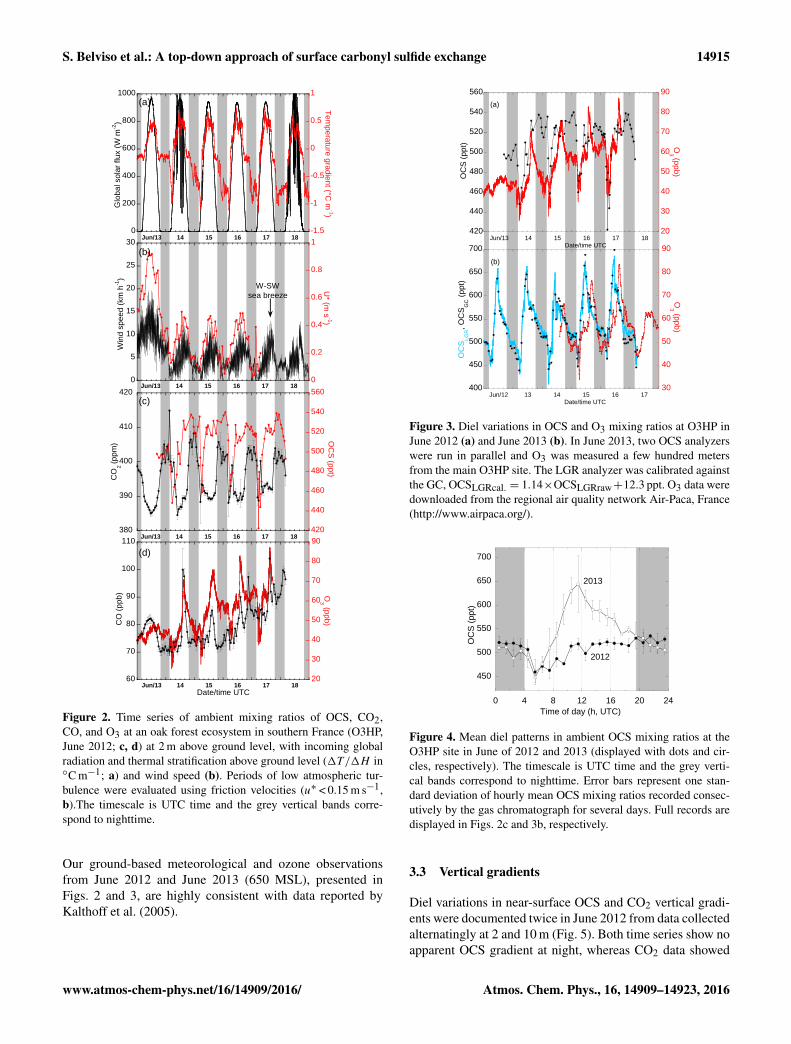
In June of 2012, CO2 presented a clear and reproduciblediurnal cycle with a maximum during the night (Fig. 2c).This maximum, an increase of 10–20 ppm, correlates to thedecrease of global radiation (Fig. 2a). This increase oc-curred between the period of maximum atmospheric turbu-lence (u∗ > 0.4 m s−1, Fig. 2b), a few hours after the maxi-mum solar radiation (Fig. 2a), and the nocturnal period whenatmospheric turbulence is reduced (u∗ < 0.2 m s−1, Fig. 2b)and strong temperature gradients above ground level form(∼−0.5 ◦C m−1, Fig. 2a). The temperature gradient is aproxy of low atmospheric mixing and boundary layer stabil-ity. During this period, the variability in OCS was relativelylow as compared to CO2 (10 ppt at the most). The strongesttemperature gradients above ground level (∼−1 ◦C m−1,Fig. 2a) were observed after sunrise (04:00 UTC), for about2 h. The diel cycle in the atmospheric boundary layer exhib-ited a much steeper decline in OCS after sunrise than at night(Fig. 2c); the same holds for ozone (Fig. 2d). The ampli-

tude of the early morning drop of OCS was in the 60–100 pptrange. That of O3 was in the range of 15–30 ppb. It is worthnoting that the large nocturnal maximum of CO2 was fol-lowed by a secondary one in the early morning but of shorterduration and smaller amplitude (10 ppm at the most, Fig. 2c).Hence, important variations in CO2 were observed during theperiod of lowest OCS concentrations. In general, OCS andO3 diel variations were in phase except in the late afternoonwhen we never observed a peak of OCS associated with thepeaks of O3 and CO (Figs. 3a and 2d).

Figure 4 compares the mean diel patterns in ambient OCSmixing ratios at 2 m height in June 2012 and June 2013, con-structed from data presented in Figs. 2c and 3b, respectively.Data show that the OCS concentrations were more stable atnight than during the day since a drop of ∼ 50 ppt was ob-served in the early morning hours, down to ∼ 450 ppt, fol-lowed by a rise up to∼ 520 ppt in June 2012 and∼ 650 ppt inJune 2013. These huge diurnal variations, with amplitudes inthe range of 150–250 ppt (Fig. 3b), were confirmed by inde-pendent measurements carried out with the LGR CO2–OCS–CO–H2O analyzer, which was running in parallel (Fig. 3b).The concomitant decrease of OCS and O3 in the early morn-ing hours was confirmed in the 2013 records (Fig. 3b). Fur-thermore, the air masses richest in O3, which were trans-ported over O3HP by strong winds in the late afternoon, werenot the richest in OCS throughout the campaign (Fig. 3b).



0

200

400

600

800

1000

-1.5

-1

-0.5

0

0.5

1

Jun/13 14 15 16 17 18

Glo

bal s

olar

flux

(W

m-2

)

Tem

perature gradient (°C m

-1)

0

5

10

15

20

25

30

0

0.2

0.4

0.6

0.8

1

Jun/13 14 15 16 17 18

Win

d sp

eed

(km

h-1

)

U* (m

s-1)

W-SWsea breeze

380

390

400

410

420

420

440

460

480

500

520

540

560

Jun/13 14 15 16 17 18

CO

2 (p

pm)

OC

S (ppt)

60

70

80

90

100

110

20

30

40

50

60

70

80

90

Jun/13 14 15 16 17 18

CO

(pp

b)

Date/time UTC

O3 (ppb)

(a)

(b)

(c)

(d)

Figure 2. Time series of ambient mixing ratios of OCS, CO2,CO, and O3 at an oak forest ecosystem in southern France (O3HP,June 2012; c, d) at 2 m above ground level, with incoming globalradiation and thermal stratification above ground level (1T/1H in◦C m−1; a) and wind speed (b). Periods of low atmospheric tur-bulence were evaluated using friction velocities (u∗ < 0.15 m s−1,b).The timescale is UTC time and the grey vertical bands corre-spond to nighttime.

Our ground-based meteorological and ozone observationsfrom June 2012 and June 2013 (650 MSL), presented inFigs. 2 and 3, are highly consistent with data reported byKalthoff et al. (2005).

420

440

460

480

500

520

540

560

20

30

40

50

60

70

80

90

Jun/13 14 15 16Date/time UTC

17 18

OC

S (

ppt) O

3 (ppb)

400

450

500

550

600

650

700

30

40

50

60

70

80

90

Jun/12 13 14 15Date/time UTC

16 17

OC

SLG

R, O

CS

GC (

ppt)

O3 (ppb)

(a)

(b)

Figure 3. Diel variations in OCS and O3 mixing ratios at O3HP inJune 2012 (a) and June 2013 (b). In June 2013, two OCS analyzerswere run in parallel and O3 was measured a few hundred metersfrom the main O3HP site. The LGR analyzer was calibrated againstthe GC, OCSLGRcal. = 1.14×OCSLGRraw+12.3 ppt. O3 data weredownloaded from the regional air quality network Air-Paca, France(http://www.airpaca.org/).

450

500

550

600

650

700

0 4 8 12 16 20 24

OC

S (

ppt)

Time of day (h, UTC)

2013

2012

Figure 4. Mean diel patterns in ambient OCS mixing ratios at theO3HP site in June of 2012 and 2013 (displayed with dots and cir-cles, respectively). The timescale is UTC time and the grey verti-cal bands correspond to nighttime. Error bars represent one stan-dard deviation of hourly mean OCS mixing ratios recorded consec-utively by the gas chromatograph for several days. Full records aredisplayed in Figs. 2c and 3b, respectively.

3.3 Vertical gradients

Diel variations in near-surface OCS and CO2 vertical gradi-ents were documented twice in June 2012 from data collectedalternatingly at 2 and 10 m (Fig. 5). Both time series show noapparent OCS gradient at night, whereas CO2 data showed


http://www.airpaca.org/


420

440

460

480

500

520

540

560

380

390

400

410

420

8 10 12 14Jun/6

16 18 20 22 0 2 4Jun/7

6 8

OC

S (

pp

t)

CO

2 (pp

m)

10 m

2 m

10 m

2 m

460

480

500

520

540

390

395

400

405

410

8 10 12 14Jun/17

16 18 20 22 0 2 4Jun/18

6 8Date/time UTC

OC

S (

pp

t)

CO

2 (pp

m)

10 m

2 m

10 m

2 m

(a)

(b)

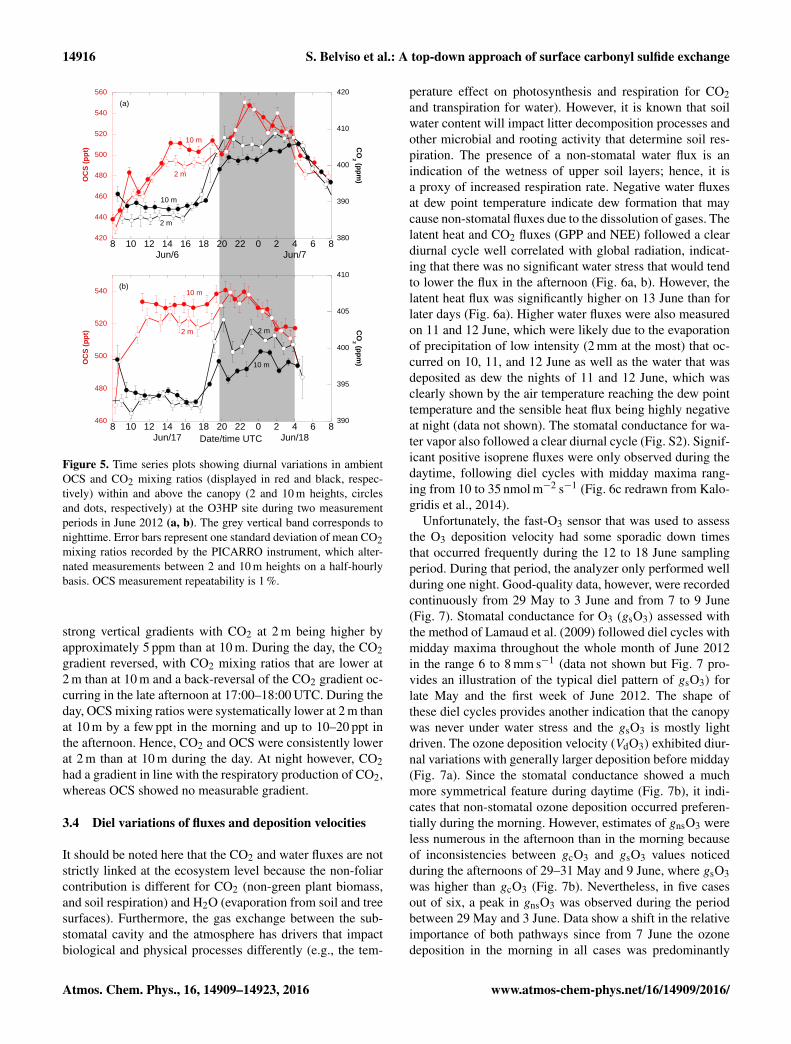
Figure 5. Time series plots showing diurnal variations in ambientOCS and CO2 mixing ratios (displayed in red and black, respec-tively) within and above the canopy (2 and 10 m heights, circlesand dots, respectively) at the O3HP site during two measurementperiods in June 2012 (a, b). The grey vertical band corresponds tonighttime. Error bars represent one standard deviation of mean CO2mixing ratios recorded by the PICARRO instrument, which alter-nated measurements between 2 and 10 m heights on a half-hourlybasis. OCS measurement repeatability is 1 %.

strong vertical gradients with CO2 at 2 m being higher byapproximately 5 ppm than at 10 m. During the day, the CO2gradient reversed, with CO2 mixing ratios that are lower at2 m than at 10 m and a back-reversal of the CO2 gradient oc-curring in the late afternoon at 17:00–18:00 UTC. During theday, OCS mixing ratios were systematically lower at 2 m thanat 10 m by a few ppt in the morning and up to 10–20 ppt inthe afternoon. Hence, CO2 and OCS were consistently lowerat 2 m than at 10 m during the day. At night however, CO2had a gradient in line with the respiratory production of CO2,whereas OCS showed no measurable gradient.

3.4 Diel variations of fluxes and deposition velocities

It should be noted here that the CO2 and water fluxes are notstrictly linked at the ecosystem level because the non-foliarcontribution is different for CO2 (non-green plant biomass,and soil respiration) and H2O (evaporation from soil and treesurfaces). Furthermore, the gas exchange between the sub-stomatal cavity and the atmosphere has drivers that impactbiological and physical processes differently (e.g., the tem-

perature effect on photosynthesis and respiration for CO2and transpiration for water). However, it is known that soilwater content will impact litter decomposition processes andother microbial and rooting activity that determine soil res-piration. The presence of a non-stomatal water flux is anindication of the wetness of upper soil layers; hence, it isa proxy of increased respiration rate. Negative water fluxesat dew point temperature indicate dew formation that maycause non-stomatal fluxes due to the dissolution of gases. Thelatent heat and CO2 fluxes (GPP and NEE) followed a cleardiurnal cycle well correlated with global radiation, indicat-ing that there was no significant water stress that would tendto lower the flux in the afternoon (Fig. 6a, b). However, thelatent heat flux was significantly higher on 13 June than forlater days (Fig. 6a). Higher water fluxes were also measuredon 11 and 12 June, which were likely due to the evaporationof precipitation of low intensity (2 mm at the most) that oc-curred on 10, 11, and 12 June as well as the water that wasdeposited as dew the nights of 11 and 12 June, which wasclearly shown by the air temperature reaching the dew pointtemperature and the sensible heat flux being highly negativeat night (data not shown). The stomatal conductance for wa-ter vapor also followed a clear diurnal cycle (Fig. S2). Signif-icant positive isoprene fluxes were only observed during thedaytime, following diel cycles with midday maxima rang-ing from 10 to 35 nmol m−2 s−1 (Fig. 6c redrawn from Kalo-gridis et al., 2014).

Unfortunately, the fast-O3 sensor that was used to assessthe O3 deposition velocity had some sporadic down timesthat occurred frequently during the 12 to 18 June samplingperiod. During that period, the analyzer only performed wellduring one night. Good-quality data, however, were recordedcontinuously from 29 May to 3 June and from 7 to 9 June(Fig. 7). Stomatal conductance for O3 (gsO3) assessed withthe method of Lamaud et al. (2009) followed diel cycles withmidday maxima throughout the whole month of June 2012in the range 6 to 8 mm s−1 (data not shown but Fig. 7 pro-vides an illustration of the typical diel pattern of gsO3) forlate May and the first week of June 2012. The shape ofthese diel cycles provides another indication that the canopywas never under water stress and the gsO3 is mostly lightdriven. The ozone deposition velocity (VdO3) exhibited diur-nal variations with generally larger deposition before midday(Fig. 7a). Since the stomatal conductance showed a muchmore symmetrical feature during daytime (Fig. 7b), it indi-cates that non-stomatal ozone deposition occurred preferen-tially during the morning. However, estimates of gnsO3 wereless numerous in the afternoon than in the morning becauseof inconsistencies between gcO3 and gsO3 values noticedduring the afternoons of 29–31 May and 9 June, where gsO3was higher than gcO3 (Fig. 7b). Nevertheless, in five casesout of six, a peak in gnsO3 was observed during the periodbetween 29 May and 3 June. Data show a shift in the relativeimportance of both pathways since from 7 June the ozonedeposition in the morning in all cases was predominantly



-25

-20

-15

-10

-5

0

5

10

Jun/13 14 15 16 17Rec

o, G

PP

, NE

E (

µm

ol m

s)

-2-1

0

10

20

30

40

Jun/13 14 15Date/time UTC

16 17

Isop

rene

flux

(nm

ol m

-2 s

-1)

0

200

400

600

800

1000

Jun/13 14 15 16 17

RgLEH

Ene

rgy

fluxe

s (W

m-2

) (a)

(b)

(c)

Figure 6. A 4-day time series of (a) global radiation (Rg), sensi-ble and latent heat (H and LE), and of CO2 hourly fluxes fromeddy covariance data measured at the O3HP site (b, June 2012).Reco, GPP, and NEE fluxes stand for ecosystem respiration, grossprimary production, and net ecosystem exchange, respectively. Weuse the convention that negative values of fluxes indicate carbon up-take by the forest ecosystem. Panel (c) displays the isoprene fluxesmeasured concomitantly by the disjunct eddy covariance technique(Kalogridis et al., 2014).

through the stomatal pathway. Unfortunately, we have no in-dication about ozone deposition pathways during the peri-ods where OCS was monitored in the atmosphere. However,the shift towards higher O3 deposition through the stomatalpathway during the second week of June (Fig. 7b) and thestrong similarities between OCS and O3 diurnal patterns inJune 2012 (Fig. 3a) suggest that the non-stomatal pathwaylost importance throughout the month of June.

4 Discussion

4.1 Role of atmospheric dynamics in OCS exchange

OCS diel variations presented here (Fig. 3) resemble thosereported by Berkelhammer et al. (2014) at two sites in centralNorth America where steep rises in OCS also occurred aftersunrise (see their Figs. 7b and S11). The authors suggestedthat this morning rise was related to boundary layer dynam-ics when air from above, richer in OCS than the air from thenocturnal boundary layer, was entrained downwards. This is

0

5

10

15

20

25

30

May/29 30 31 Jun/1 2 3 7 8 9

Con

duct

ance

s (m

m s

-1)

Date/time UTC

gcO3

gsO3

gnsO3

0

5

10

15

20

May/29 30 31 Jun/1 2 3 7 8 9

VdO

3 (m

m s

-1)

(a)

(b)

Figure 7. Diel variations in (a) ozone deposition velocity (VdO3),(b) canopy conductance (gcO3), stomatal conductance (gsO3), andnon-stomatal conductance (gnsO3) from 29 May to 9 June in 2012.The partitioning was obtained with the Lamaud et al. (2009) ap-proach (see text for details).

also the case at O3HP as shown in the vertical profiles ofwater vapor (Fig. S3). Entrainment of dry air from the noc-turnal boundary layer is evidenced by the decrease in watervapor concentrations about 2 h after sunrise. This decreaseis generally more important at 10 m than at 2 m. However,diurnal variations with amplitudes over 200 ppt as observedat the O3HP in June 2013 were never reported before. Thisraises the question of the origin of air masses rich in OCS ad-vected over O3HP in mid-June 2013. It is highly unlikely thatlong-range transport of biomass burning gases and aerosolsbetween North America and the Mediterranean region wasresponsible for OCS contamination because the transport ofbiomass burning material occurred in late June 2013 after theend of our OCS surveys (see Fig. 4 in Ancellet et al., 2016).Since the O3-rich air masses that reach the O3HP in the lateafternoon lag behind those rich in OCS by ∼ 4 h (Fig. 3b),it is clear that the OCS and O3 peaks have distinct origins.Backward trajectories at 300 m above ground level endingat 12:00 UTC (Stein et al., 2015), when OCS levels at theO3HP in June 2013 were over 600 ppt (Fig. 3b), show thatthe circulation of the air masses during the 2012 and 2013periods was at low altitude (below about 500 m a.g.l., i.e., be-low 1100 m a.s.l.); thus, they were generally in the boundarylayer. The back trajectories show that the air masses werein closer contact with the continent in June 2013 than inJune 2012 and that the transport in June 2013 was from theN–NW along the Rhône Valley (Fig. S4). South of the city



of Lyon, the Rhône Valley is highly industrialized, and it istherefore likely that the O3HP site is impacted by anthro-pogenic direct or indirect emissions of OCS (i.e., from theoxidation of CS2 since the largest production of CS2 in west-ern Europe is located in the Rhône Valley; Campbell et al.,2015). Polluted air very likely propagates southwards in theupper layers within the nocturnal jet, which was observedin the sodar measurements performed nearby at Cadarache(Kalthoff et al., 2005), and is entrained downwards in themorning when turbulence recovers. Moreover, we can alsodemonstrate that the source of OCS pollution is persistentlyfrom the same direction using data gathered in Fig. S5, whichshow the full June 2013 OCS record, starting from 8 June,and the corresponding back trajectories. It is clear that thereis no sign of pollution in OCS when air masses, advectedfrom the Mediterranean Sea, reach the OHP site at noon,300 m a.g.l. Finally, Fig. S6 demonstrates that advection ofpollutants from the combustion of fossil fuels (and frombiomass burning, see above) is unlikely in the OHP area ex-cept for on the night of 15 June when CO levels went up to250 ppb. A CO pollution event was also recorded the nextmorning but data show no impact on OCS levels. In the af-ternoon, polluted air from the metropolitan area of Marseilleis transported by the sea breeze thus leading to an increase ofozone at elevated layers above the convective boundary layeras demonstrated in the air circulation study of Kalthoff etal. (2005). The highest ozone concentrations above 100 ppbcan be found about 50 km further downwind north and north-east of Marseille both in the mountainous areas of Luberonand above (Kalthoff et al., 2005; see Fig. 6 of that paper).We can therefore conclude that the photosmog of the city ofMarseille is not a source of OCS.

4.2 Ecosystem relative uptake (ERU)

At the O3HP, OCS concentration gradients showing lowerconcentrations at 2 m than at 10 m were observed during thedaytime (Fig. 5), especially during the afternoon so when tur-bulent mixing was strongest (Fig. 1b). Gradients were nonex-istent at night. This implies that the forest ecosystem wasessentially a net sink of OCS. Measured CO2 vertical gra-dients indicate that the forest ecosystem was a net sink ofCO2 during the daytime and a net source at night, featuresthat were confirmed by the eddy covariance data showingNEE to range between −15 and −20 µ mol m−2 s−1 aroundmidday and 0–5 µ mol m−2 s−1 at night (Fig. 6). However,the sharp rise in OCS concentrations between 06:00 and12:00 UTC (Fig. 2) and the reversal of the CO2 gradientsat 17:00–18:00 UTC (Fig. 5) reduce the time window to afew hours in the afternoon where the ecosystem relative up-take of OCS (ERU), which is the ratio of the relative verticalgradients of OCS and CO2, can be assessed. ERU is an im-portant parameter since it is proportional to GPP and NEEscaled by the ratio of relative leaf exchange rates (LRU) fol-lowing Eq. (2). Therefore, we anticipate that this approach to

partition measured NEE will hardly be applicable at O3HP,not only because the amplitude of the diurnal variations inLRU is unknown at O3HP but also because vertical gradientsof OCS cannot be calculated from measurements carried outthroughout the whole period of illumination. In 2012, onlydata collected in the afternoon were exploitable and the meanOCS /CO2 ratio at 2 m height was 1.33± 0.02 ppt ppm−1,n= 27. In June 2013, polluted air masses produced dramaticvariation in atmospheric OCS /CO2 ratios in the morningand the afternoon, leaving no time window for ERU calcula-tion. These air masses were not related to urban photosmogepisodes since there was a gap of ∼ 4 h between the peaksof OCS (up to 700 ppt) and O3 (up to 85 ppb). With thesecaveats in mind, the ratio of the mean relative vertical gra-dients of OCS and CO2 (calculated from linear OCS pro-files) was equal to 4.7 and 4.3 for the afternoons of 6 and17 June, respectively. However, it had a large relative error(≥ 50 %) and was consistent with ERUs reported by Blon-quist et al. (2011) at the Harvard Forest AmeriFlux site insummer–autumn 2006 (5.7± 1.2 (1 SD) for short-term ERUvalues calculated from linear OCS profiles as we did at theO3HP).

Only when the plant uptake is the dominant flux, is theERU proportional to the ratio of GPP /NEE, with a propor-tionality constant that is the LRU (Campbell et al., 2008).As discussed above, this is only the case at the O3HP sitefor a few hours in the afternoon (because at other momentsthe ecosystem is not the main driver but rather part of theboundary layer dynamics) and that ERU could only be calcu-lated using the OCS and CO2 gradients for these few hours.When ERUs and the mean NEE /GPP ratio calculated forthe period 12:00–17:00 UTC (0.78± 0.05, n= 20) are usedin Eq. (2), LRUs at the O3HP are equal to 3.7 and 3.4. Thesevalues fall in the upper range of LRUs obtained from leafchamber studies over a large range of light conditions andtree species (1–4, Stimler et al., 2010; 1.3–2.3, Berkelham-mer et al., 2014).

4.3 Relative role of plants and soil in OCS exchange

Our OCS measurements were carried out during the periodof maximum gross primary productivity of Mediterraneanoak forests (Allard et al., 2008; Maselli et al., 2014). Atthe O3HP, the maximum of Q. pubescens net photosyn-thetic assimilation also occurs in June (Genard-Zielinski etal., 2015). The O3HP site appears to be ideal for the useof OCS uptake by plants as a tracer for GPP in a Mediter-ranean oak forest because the soil is neither a source nor asink of OCS when GPP fluxes culminate. The lack of net up-take of OCS at night is a specific feature of the O3HP sitethat is not shared by other open oak woodlands character-ized by a Mediterranean climate (Kuhn et al., 1999; Sun etal., 2015). The study of Kuhn et al. (1999) was performedin June 1994 at the Hastings Natural History Reservationin Monterey County, central coastal California (490 m a.s.l.),



which is located in a side valley of the Carmel Valley, ap-proximately 40 km from the coast. These authors reported anocturnal drop in the OCS ambient mixing ratio by about150 ppt corresponding to a nocturnal OCS deposition rate ofup to −7.6 pmol m−2 s−1, which was estimated by a noctur-nal boundary layer depletion model. The range of fluxes re-ported by Kuhn et al. (1999) is consistent with those mea-sured using soil chambers at Stunt Ranch in southern Cali-fornia in April 2013 (0.1 to −6.5 pmol m−2 s−1; Sun et al.,2015). OCS fluxes at Stunt Ranch exhibited clear diurnalvariations with higher uptakes during the night than duringthe day (Sun et al., 2015). Unfortunately, the signature ofthese fluxes in the nocturnal boundary layer in terms of noc-turnal drop in OCS mixing ratio was not reported in that pa-per. To give an illustration of what might be the atmosphericsignature during stable nocturnal conditions of OCS uptakeevents of such intensity, we extracted data from a set of ob-servations where the role that soil, leaf, and atmospheric dy-namics have on surface OCS exchange is investigated fromOCS diurnal cycles (as at O3HP) and nocturnal fluxes cal-culated using the radon-tracer method (Belviso et al., 2013).Figure S7 shows an 8-day time series of ambient mixing ra-tios of OCS, CO2, CO, and O3 carried out in mid-April 2015(after bud break and almost complete leaf expansion) in asuburban area of the Saclay Plateau (Paris region) in relationto incoming global radiation, thermal stratification, and windspeed (as at the O3HP). Periods of low atmospheric turbu-lence over the Saclay Plateau were evaluated using 222Rn ac-cumulations. In April 2015, hourly variations show nighttimeand early morning decreases of OCS mixing ratios (Fig. S7c)and corresponding 222Rn increases (Fig. S7b). The amplitudeof OCS diurnal variations is in the 40–80 ppt range. OCSminima coincide with calm meteorological conditions withwind velocities lower than 6 km h−1 (Fig. S7b), which arefavorable to thermal stratification (Fig. S7a), with CO2 max-ima sometime up to ∼ 480 ppm (Fig. S7c) and with O3 min-ima down to a few ppb (Fig. S7d). However, it is worth notinghere that the amplitude of CO2 and O3 nocturnal variationsover the Saclay Plateau in early spring are higher than thoseat O3HP due to anthropogenic emissions of CO2, which canbe traced using CO mixing ratios (Fig. S7d), and to NOxemissions, which accelerate the chemical removal of O3 (O3reacts with NO, data not shown). OCS fluxes calculated us-ing the radon-tracer method during stable nocturnal condi-tions ranged from −4.8 pmol m−2 s−1 (night of 14 April) to−14.2 pmol m−2 s−1 (night of 11 April, Fig. S7c). They fallin the upper range of fluxes reported by Kuhn et al. (1999)and Sun et al. (2015), but the comparison should be madewith caution because three different methods were used toestimate the OCS fluxes (i.e., a boundary layer model, soilchambers, and the radon-tracer method). Qualitatively, it isclear that uptake rates of several pmol m−2 s−1 lead to dropsin the OCS ambient mixing ratio by several tens of ppt duringperiods of low atmospheric turbulence. Hence, a major dif-ference between these woodlands and the O3HP site during

springtime is that soil of the Mediterranean forest ecosystemof southern France is not a net sink of OCS. Soil OCS up-take has been shown to be dependent on soil physical proper-ties like soil structure, water content, water-filled pore space,and temperature (Van Diest and Kesselmeier, 2008; Ogée etal., 2016) but also on soil biological properties like micro-bial activity (Kato et al., 2008; Ogawa et al., 2013), activeroot density (Maseyk et al., 2014), or the presence of a lit-ter layer (Berkelhammer et al., 2014; Sun et al., 2015). Awayfrom a range of optimum uptake, which varies between soils,changes in soil water content and temperature can markedlyreduce OCS uptake by soils (Van Diest and Kesselmeier,2008). However, the soil temperature and water content atthe O3HP (Fig. 1c, d) are typically in the range of optimumuptake published by Van Diest and Kesselmeier (2008). Alimitation of OCS uptake by soils due to a poor OCS dif-fusion is also unlikely considering that the soils from theO3HP are strongly structured and are far from being watersaturated. Finally, the only physical property of soil differingamong the three open oak woodlands is the soil texture, witha fine clayey texture at the O3HP but a coarse sandy loamtexture at Hastings Reservation (Kuhn et al., 1999) and atstunt Ranch (Sun et al., 2015). OCS uptake by fine-texturedsoils has already been reported (Maseyk et al., 2014), thisresult pointed out the need for measurements of OCS up-take for a greater diversity of soils. Concerning the biologi-cal soil properties, the soil at the O3HP is covered by a rel-atively thick litter layer that may induce a change from OCSuptake to OCS emission (Berkelhammer et al., 2014). How-ever, at Stunt Ranch Sun et al. (2015) measured that the lit-ter was responsible for OCS uptake. The surface horizons atthe O3HP showed organic carbon content ranging from 167to 43 g kg−1 in the surface soil horizons (Table 1) but only24 g kg−1 at Hastings Reservation (no data on soil organiccarbon are available for Stunt Ranch). Being richer in organiccarbon, soils at the O3HP show very likely higher microbialactivity, a factor that should stimulate uptake of OCS by soilsbut apparently does not. If the capacity of soils to consumeOCS is more related to specific enzymatic activities (car-bonic anhydrase (CA) and OCS hydrolase) than to the gen-eral variables presented above, our observations would high-light deficiencies in these enzymatic activities in the calcium-carbonate-rich soils of O3HP. However, this hypothesis is notconsistent with the suggestion that CA performs an essen-tial role in microbial organisms surviving periods of osmoticstress such as drought at the surface of Mediterranean soils(Wingate et al., 2008). Finally, as roots and associated rhizo-sphere have been found to produce OCS, a greater abundanceof roots in the surface soils at O3HP by comparison with thetwo other oak woodlands may explain why the soils at O3HPare not a sink of OCS. In other words, the lack of nocturnalnet uptake of OCS would indicate that gross consumption ofthis gas in soil is compensated for by emission processes thatremain to be characterized. However, no data on root abun-



dance are available at Hastings Reservation or Stunt Ranchto confirm such a hypothesis.

4.4 Potential use of OCS to partition ozone decay nearthe ground

Data show strong similarities during the night and earlymorning hours between OCS and O3 diel variations at theO3HP suggesting a similar sink during that period (Fig. 3).At the O3HP, volatile organic compounds (VOCs) producedby the vegetation are essentially in the form of isoprene(Kalogridis et al., 2014; Genard-Zielinski et al., 2015). Iso-prene is oxidized in the atmosphere by the hydroxyl radi-cal (OH), O3, and the nitrate radical (NO3), but in-canopychemical oxidation of isoprene at the O3HP was found tobe weak and did not seem to have a significant impact onisoprene concentrations and fluxes above the canopy (Kalo-gridis et al., 2014). Hence, ozone deposition at the O3HP wasessentially through leaf uptake via stomata and surface depo-sition, without a strong contribution from chemical reactions.In late May and early June 2012, the non-stomatal contribu-tion to the ozone flux was in general markedly higher than thestomatal one in the morning hours (before 10:00 UTC), butit became much less significant in the afternoon (Fig. 7b).Conversely, during the second week of June, although therewere still signs of non-stomatal loss of ozone in the morn-ing, the major contribution to ozone deposition was throughthe stomatal pathway (Fig. 7b). The analogy with OCS atnighttime and in the early morning suggests that soil didnot contribute much to the O3 flux and that the depositionflux of O3 in mid-June was essentially the result of leaf up-take. However, it is difficult to evaluate the soil ozone path-ways without turbulence measurements inside the canopy. Itwould be worth looking further into how OCS could be usedto partition ozone fluxes near the ground between soil andleaf deposition processes. The applicability of OCS to char-acterize the strength of ozone sinks would be reduced in sit-uations where NOx would significantly impact the chemicalproduction or destruction of ozone in the canopy or whenbackground air is contaminated by primary or secondary an-thropogenic sources of OCS (Fig. 3b).

5 Conclusions and perspectives

Diel changes in the OCS mixing ratio and in its vertical distri-bution show that net soil exchange of OCS is negligible com-pared to the uptake of the gas through the stomata, a featurethat is not shared by other oak woodland ecosystems charac-terized by a Mediterranean climate. Hence, O3HP would bethe adequate place to support the installation of a monitoringstation of OCS uptake by plants from eddy covariance mea-surements in the Mediterranean region. However, the assess-ment of GPP from measured OCS fluxes at the ecosystemscale remains a tributary of our poor knowledge of LRU diel

variations at the O3HP, which requires further examinationusing new experimental facilities (branch chambers or bagsand/or coupled NEE–ERU measurements). In the frameworkof the European infrastructure Integrated Carbon Observa-tion System (ICOS), an atmospheric measurement station(100 m high tower) was set up at OHP in 2014 to determinemultiyear records of greenhouse gases. Future research onthe ERU is encouraged by the site being suitable to performcontinuous and high-precision vertical profiles of OCS us-ing quantum cascade laser spectrometry. Unfortunately, ourpreliminary surveys suggest that the site is less adequate forscaling NEE to GPP from observations of vertical gradientsof OCS relative to CO2 during the daytime than for estimat-ing GPP directly from eddy covariance measurements; thetime window for calculation of the ecosystem relative up-take of OCS was found to be restricted to a few hours aftermidday at the O3HP (1) because in the morning the verticaldistribution of OCS is disrupted by entrainment of OCS-richtropospheric air sometimes contaminated by anthropogenicemissions and (2) because the CO2 vertical gradient reverseswhen it is still light.

6 Data availability

The data have been deposited in the CNRS Archivesas a zip file and can be downloaded from: https://mycore.core-cloud.net/public.php?service=files&t=04c569376fa8ca82e5ebdf09cd18630d (Belviso et al., 2016).

The Supplement related to this article is available onlineat doi:10.5194/acp-16-14909-2016-supplement.

Acknowledgements. We are grateful for the support of the adminis-trative and technical staff of the “Observatoire de Haute-Provence”and the “Institut Mediterranéen de Biodiversité et Ecologie terrestreet marine” and support from the OHP infrastructure. We are alsograteful to Eric Lamaud and Jean-Marc Bonnefond from INRAfor lending the NOAA ozone analyzer and the Li7500 CO2/H2OIRGA. The authors express their thanks to the staff of the SIRTAobservatory, which provided access to meteorological data. The au-thors gratefully acknowledge the NOAA Air Resources Laboratory(ARL) for the provision of the HYSPLIT transport and dispersionmodel and/or READY website (http://www.ready.noaa.gov) used inthis publication. This work was supported by the French NationalAgency for Research (ANR 2010 JCJC 603 01 CANOPÉE). Wealso thank the EU FP7 ECLAIRE project for funding. The purchaseof the LGR OCS, CO2, H2O, and CO analyzer used during the2013 field campaign was co-funded by PACA region, GIS IBiSA,CEA, CNRS, and FR 3098 ECCOREV (IMAPLANT project toB.G.).

Edited by: M. KanakidouReviewed by: three anonymous referees


https://mycore.core-cloud.net/public.php?service=files&t=04c569376fa8ca82e5ebdf09cd18630d



http://dx.doi.org/10.5194/acp-16-14909-2016-supplement

http://www.ready.noaa.gov


References

Allard, V., Ourcival, J. M., Rambal, S., Joffre, R., and Ro-cheteau, A.: Seasonal and annual variation of carbon ex-change in an evergreen Mediterranean forest in southernFrance, Glob. Change Biol., 14, 714–725, doi:10.1111/j.1365-2486.2008.01539.x, 2008.

Ammann, C., Brunner, A., Spirig, C., and Neftel, A.: Technicalnote: Water vapour concentration and flux measurements withPTR-MS, Atmos. Chem. Phys., 6, 4643–4651, doi:10.5194/acp-6-4643-2006, 2006.

Ancellet, G., Pelon, J., Totems, J., Chazette, P., Bazureau, A.,Sicard, M., Di Iorio, T., Dulac, F., and Mallet, M.: Long-rangetransport and mixing of aerosol sources during the 2013 NorthAmerican biomass burning episode: analysis of multiple lidarobservations in the western Mediterranean basin, Atmos. Chem.Phys., 16, 4725–4742, doi:10.5194/acp-16-4725-2016, 2016.

Arora, V. K. and Boer, G. J.: Terrestrial ecosystems response tofuture changes in climate and atmospheric CO2 concentration,Biogeosciences, 11, 4157–4171, doi:10.5194/bg-11-4157-2014,2014.

Asaf, D., Rotenberg, E., Tatarinov, F., Dicken, U., Montzka, S.A., and Yakir, D.: Ecosystem photosynthesis inferred from mea-surements of carbonyl sulphide flux, Nat. Geosci. 6, 186–190,doi:10.1038/NGEO1730, 2013.

Aubinet, M., Grelle, A., Ibrom, A., Rannik, U., Moncrieff, J., Fo-ken, T., Kowalski, A. S., Martin, P. H., Berbigier, P., Bernhofer,C., Clement, R., Elbers, J., Granier, A., Grunwald, T., Morgen-stern, K., Pilegaard, K., Rebmann, C., Snijders, W.,Valentini, R.,and Vesala, T.: Estimates of the annual net carbon and water ex-change of forests: The EUROFLUX methodology, Adv. Ecol.Res., 30, 113–175, 2000.

Bassin, S., Calanca, P., Weidinger, T., Gerosa, G., and Fuhrer,E.: Modeling seasonal ozone fluxes to grassland and wheat:model improvement, testing, and application, Atmos. Environ.,38, 2349–2359, doi:10.1016/j.atmosenv.2003.11.044, 2004.

Belviso, S., Schmidt, M., Yver, C., Ramonet, M., Gros, V.,and Launois, T.: Strong similarities between nighttime de-position velocities of carbonyl sulphide and molecular hy-drogen inferred from semi-continuous atmospheric observa-tions in Gif-sur-Yvette, Paris region, Tellus B, 65, 20719,doi:10.3402/tellusb.v65i0.20719, 2013.

Belviso, S., Gros, V., Delmotte M., Reiter, I. M., Genty, B.,and Loubet, B.: DATA_Belviso_ACP_2016, available at:https://mycore.core-cloud.net/public.php?service=files&t=04c569376fa8ca82e5ebdf09cd18630d, last access: 30 Novem-ber 2016.

Berkelhammer, M., Asaf, D., Still, C., Montzka, S., Noone, D.,Gupta, M., and Yakir, D.: Constraining surface carbon fluxes us-ing in situ measurements of carbonyl sulfide and carbon dioxide,Global Biogeochem. Cy., 28, 161–179, 2014.

Berry, J., Wolf, A., Campbell, J. E., Baker, I., Blake, N., Blake, D.,and Zhu, Z.: A coupled model of the global cycles of carbonylsulfide and CO2: A possible new window on the carbon cycle, J.Geophys. Res.-Biogeo., 118, 842–852, doi:10.1002/jgrg.20068,2013.

Blonquist Jr., J. M., Montzka, S. A., Munger, J. W., Yakir, D., Desai,A. R., Dragoni, D., Griffis, T. J., Monson, R. K., Scott, R. L., andBowling, D. R.: The potential of carbonyl sulfide as a proxy for

gross primary production at flux tower sites, J. Geophys. Res.,116, G04019, doi:10.1029/2011JG001723, 2011.

Brêthes, A., Brun, J. J., Jabiol, B., Ponge, J. F., and Toutain, F.:Classification of forest humus forms: a French proposal, Ann.Sci. Forest., 52, 6, 535–546, 1995.

Brown, K. A. and Bell, J. N. B.: Vegetation – the missing sink inthe global cycle of carbonyl sulphide (COS), Atmos. Environ.20, 537–540, 1986.

Campbell, J. E., Carmichael, G. R., Chai, T., Mena-Carrasco, M.,Tang, Y., Blake, D. R., Blake, N. J., Vay, S. A., Collatz, G. J.,Baker, I., Berry, J. A., Montzka, S. A., Sweeney, C., Schnoor,J. L., and Stanier, C. O.: Photosynthetic control of atmosphericcarbonyl sulfide during the growing season, Science, 322, 1085–1088, doi:10.1126/science.1164015, 2008.

Campbell, J. E., Whelan, M. E., Seibt, U., Smith, S. J.,Berry, J. A., and Hilton, T. W.: Atmospheric carbonyl sul-fide sources from anthropogenic activity: Implications for car-bon cycle constraints, Geophys. Res. Lett., 42, 3004–3010,doi:10.1002/2015GL063445, 2015.

Commane, R., Meredith, L. K., Baker, I. T., Berry, J. A., Munger, J.W., Montzka, S. A., Templer, P. H., Juice, S. M., Zahniser, M. S.,and Wofsy, S. C.: Seasonal fluxes of carbonyl sulfide in a mid-latitude forest, P. Natl. Acad. Sci. USA, 112, 46, 14162–14167,doi:10.1073/pnas.1504131112, 2015.

Cros, B., Durand, P., Cachier, H., Drobinski, P., Fréjafon, E.,Kottmeier, C., Perros, P. E., Peuch, V.-H., Ponche, J.-L., Robin,D., Saïd, F., Toupance, G., and Wortham, H.: The ESCOMPTEprogram: an overview, Atmos. Res., 69, 241–279, 2004.

Genard-Zielinski, A.-C., Boissard, C., Fernandez, C., Kalogridis,C., Lathière, J., Gros, V., Bonnaire, N., and Ormeño, E.: Vari-ability of BVOC emissions from a Mediterranean mixed forestin southern France with a focus on Quercus pubescens, Atmos.Chem. Phys., 15, 431–446, doi:10.5194/acp-15-431-2015, 2015.

Goldan, P. D., Fall, R., Kuster, W. C., and Fehsenfeld, F. C.: Up-take of COS by growing vegetation: a major tropospheric sink, J.Geophys. Res., 93, 14186–14192, 1988.

Hilton, T. W., Zumkehr A., Kulkarni, S., Berry, J. A., Whe-lan, M. E., and Campbell, J. E.: Large variability in ecosys-tem models explains a critical parameter for quantifyingGPP with atmospheric carbonyl sulfide, Tellus B, 67, 26329,doi:10.3402/tellusb.v67.26329, 2015.

IUSS Working Group WRB: World Reference Base for Soil Re-sources 2014. International soil classification system for namingsoils and creating legends for soil maps. World Soil ResourcesReports No. 106. FAO, Rome, Italy, 2014.

Kalogridis, C., Gros, V., Sarda-Esteve, R., Langford, B., Loubet, B.,Bonsang, B., Bonnaire, N., Nemitz, E., Genard, A.-C., Boissard,C., Fernandez, C., Ormeño, E., Baisnée, D., Reiter, I., and Lath-ière, J.: Concentrations and fluxes of isoprene and oxygenatedVOCs at a French Mediterranean oak forest, Atmos. Chem.Phys., 14, 10085–10102, doi:10.5194/acp-14-10085-2014, 2014.

Kalthoff, N., Kottmeier, C., Thürauf, J., Corsmeier, U., Saïd, F.,Fréjafon, E., and Perros, P. E.: Mesoscale circulation systemsand ozone concentrations during ESCOMPTE: a case study fromIOP 2b, Atmos. Res., 74, 355–380, 2005.

Kato, H., Saito, M., Nagahata, Y., and Katayama, Y.: Degradation ofambient carbonyl sulfide by Mycobacterium spp. in soil, Micro-biology, 154, 249–255, doi:10.1099/mic.0.2007/011213-0, 2008.


http://dx.doi.org/10.1111/j.1365-2486.2008.01539.x

http://dx.doi.org/10.1111/j.1365-2486.2008.01539.x

http://dx.doi.org/10.5194/acp-6-4643-2006



http://dx.doi.org/10.5194/bg-11-4157-2014

http://dx.doi.org/10.1038/NGEO1730

http://dx.doi.org/10.1016/j.atmosenv.2003.11.044

http://dx.doi.org/10.3402/tellusb.v65i0.20719



http://dx.doi.org/10.1002/jgrg.20068

http://dx.doi.org/10.1029/2011JG001723

http://dx.doi.org/10.1126/science.1164015

http://dx.doi.org/10.1002/2015GL063445

http://dx.doi.org/10.1073/pnas.1504131112


http://dx.doi.org/10.3402/tellusb.v67.26329


http://dx.doi.org/10.1099/mic.0.2007/011213-0


Kooijmans, L. M. J., Uitslag, N. A. M., Zahniser, M. S., Nelson, D.D., Montzka, S. A., and Chen, H.: Continuous and high-precisionatmospheric concentration measurements of COS, CO2, CO andH2O using a quantum cascade laser spectrometer (QCLS), At-mos. Meas. Tech., 9, 5293–5314, doi:10.5194/amt-9-5293-2016,2016.

Kowalski, A. S., Loustau, D., Berbigier, P., Manca, G., Tedeschi,V., Borghetti, M., Valentini, R., Kolari, P., Berninger, F., Ran-nik, U., Hari, P., Rayment, M., Mencuccini, M., Moncrieff, J.,and Grace, J.: Paired comparisons of carbon exchange betweenundisturbed and regenerating stands in four managed forests inEurope, Glob. Change Biol., 10, 1707–1723, doi:10.1111/j.1365-2486.2004.00846.x, 2004.

Kuai, L., Worden, J. R., Campbell, J. E., Kulawik, S. S., Li, K.-F.,Lee, M., Weidner, R. J., Montzka, S. A., Moore, F. L., Berry, J.A., Baker, I., Denning, A. S., Bian, H., Bowman, K. W., Liu, J.,and Yung, Y. L.: Estimate of carbonyl sulfide tropical oceanicsurface fluxes using Aura Tropospheric Emission Spectrome-ter observations, J. Geophys. Res.-Atmos., 120, 11012–11023,doi:10.1002/2015JD023493, 2015.

Kuhn, U., Ammann, C., Wolf, A., Meixner, F. X., Andreae, M. O.,and Kesselmeier, J.: Carbonyl sulfide exchange on an ecosystemscale: soil represents a dominant sink for atmospheric COS, At-mos. Environ., 33, 995–1008, 1999.

Lamaud, E., Loubet, B., Irvine, M., Stella, P., Personne, E., and Cel-lier, P.: Partitioning of ozone deposition over a developed maizecrop between stomatal and non-stomatal uptakes, using eddy-covariance flux measurements and modelling, Agr. Forest. Me-teorol., 149, 1385–1396, doi:10.1016/j.agrformet.2009.03.017,2009.

Laothawornkitkul, J., Taylor, J. E., Paul, N. D., and Hewitt, C. N.:Biogenic volatile organic compounds in the earth system, NewPhytol., 183, 27–51, doi:10.1111/j.1469-8137.2009.02859.x,2009.

Launois, T., Peylin, P., Belviso, S., and Poulter, B.: A new modelof the global biogeochemical cycle of carbonyl sulfide – Part 2:Use of carbonyl sulfide to constrain gross primary productivity incurrent vegetation models, Atmos. Chem. Phys., 15, 9285–9312,doi:10.5194/acp-15-9285-2015, 2015.

Loubet, B., Laville, P., Lehuger, S., Larmanou, E., Fléchard, C.,Mascher, N., Genermont, S., Roche, R., Ferrara, R. M., Stella,P., Personne, E., Durand, B., Decuq, C., Flura, D., Masson, S.,Fanucci, O., Rampon, J.-N., Siemens, J., Kindler, R., Gabrielle,B., Schrumpf, M., and Cellier P.: Carbon, nitrogen and green-house gases budgets over a four years crop rotation in northernFrance, Plant Soil, 343, 109–137, 2011.

Maselli, F., Cherubini, P., Chiesi, M., Gilabert, M. A., Lombardi,F., Moreno, A., Teobaldelli, M., and Tognetti, R.: Start of thedry season as a main determinant of inter-annual Mediterraneanforest production variations, Agr. Forest. Meteorol., 194, 197–206, 2014.

Maseyk, K., Berry, J. A., Billesbach, D., Campbell, J. E.,Torn, M. S., Zahniser, M., and Seibt, U.: Sources and sinksof carbonyl sulfide in an agricultural field in the South-ern Great Plains, P. Natl. Acad. Sci. USA, 111, 9064–9069,doi:10.1073/pnas.1319132111, 2014.

Mihalopoulos, N., Bonsang, B., Nguyen, B. C., Kanakidou, M., andBelviso, S.: Field observations of carbonyl sulfide deficit near the

ground : possible implication of vegetation, Atmos. Environ., 23,2159–2166, 1989.

Montzka, S. A., Calvert, P., Hall, B. D., Elkins, J. W., Conway,T. J., Tans, P. P., and Sweeney, C.: On the global distribution,seasonality, and budget of atmospheric carbonyl sulfide (COS)and some similarities to CO2, J. Geophys. Res.-Atmos., 112,D09302, doi:10.1029/2006JD007665, 2007.

Muller, J. B. A., Percival, C. J., Gallagher, M. W., Fowler, D.,Coyle, M., and Nemitz, E.: Sources of uncertainty in eddy co-variance ozone flux measurements made by dry chemilumines-cence fast response analysers, Atmos. Meas. Tech., 3, 163–176,doi:10.5194/amt-3-163-2010, 2010.

Ogawa, T., Noguchi, K., Saito, M., Nagahata, Y., Kato, H., Ohtaki,A., Nakayama, H., Dohmae, N., Matsushita, Y., Odaka, M.,Yohda, M., Nyunoya, H., and Katayama, Y.: Carbonyl sulfide hy-drolase from Thiobacillus thioparus strain THI115 is one of theβcarbonic anhydrase family enzymes, J. Am. Chem. Soc., 135,3818–3825, doi:10.1021/ja307735e, 2013.

Ogée, J., Sauze, J., Kesselmeier, J., Genty, B., Van Diest, H.,Launois, T., and Wingate, L.: A new mechanistic framework topredict OCS fluxes from soils, Biogeosciences, 13, 2221–2240,doi:10.5194/bg-13-2221-2016, 2016.

Santonja, M., Fernandez, C., Gauquelin, T., and Baldy, B.: Climatechange effects on litter decomposition: intensive drought leads toa strong decrease of litter mixture interactions, Plant Soil, 393,69–82, 2015.

Seibt, U., Kesselmeier, J., Sandoval-Soto, L., Kuhn, U., and Berry,J. A.: A kinetic analysis of leaf uptake of COS and its relationto transpiration, photosynthesis and carbon isotope fractionation,Biogeosciences, 7, 333–341, doi:10.5194/bg-7-333-2010, 2010.

Stein, A. F., Draxler, R. R., Rolph, G. D., Stunder, B. J. B., Co-hen, M. D., and Ngan, F.: NOAA’s HYSPLIT atmospheric trans-port and dispersion modeling system, B. Am. Meteorol. Soc., 96,2059–2077, doi:10.1175/BAMS-D-14-00110.1, 2015.

Stella, P., Loubet, B., Lamaud, E., Laville, P., and Cellier, P.: Ozonedeposition onto bare soil: a new parameterisation, Agr. Forest.Meteorol., 151, 669–681, 2011.

Stimler, K., Montzka, S. A., Berry, J. A., Rudich, Y., and Yakir, D.:Relationships between carbonyl sulfide (COS) and CO2 duringleaf gas exchange, New Phytol., 186, 869–878, 2010.

Stimler, K., Berry, J. A., Montzka, S. A., and Yakir, D.: Associationbetween carbonyl sulfide uptake and 181 during gas exchange inC3 and C4 Leaves, Plant Physiol., 157, 509–517, 2011.

Sun, W., Maseyk, K., Lett, C., and Seibt, U.: A soil diffusion–reaction model for surface COS flux: COSSM v1, Geosci. ModelDev., 8, 3055–3070, doi:10.5194/gmd-8-3055-2015, 2015.

Van Diest, H. and Kesselmeier, J.: Soil atmosphere exchange of car-bonyl sulfide (COS) regulated by diffusivity depending on water-filled pore space, Biogeosciences, 5, 475–483, doi:10.5194/bg-5-475-2008, 2008.

Whelan, M. E., Hilton, T. W., Berry, J. A., Berkelhammer, M., De-sai, A. R., and Campbell, J. E.: Carbonyl sulfide exchange in soilsfor better estimates of ecosystem carbon uptake, Atmos. Chem.Phys., 16, 3711–3726, doi:10.5194/acp-16-3711-2016, 2016.

White, M. L., Zhou, Y., Russo, R. S., Mao, H., Talbot, R., Varner,R. K., and Sive, B. C.: Carbonyl sulfide exchange in a temperateloblolly pine forest grown under ambient and elevated CO2, At-mos. Chem. Phys., 10, 547–561, doi:10.5194/acp-10-547-2010,2010.


http://dx.doi.org/10.5194/amt-9-5293-2016

http://dx.doi.org/10.1111/j.1365-2486.2004.00846.x

http://dx.doi.org/10.1111/j.1365-2486.2004.00846.x

http://dx.doi.org/10.1002/2015JD023493

http://dx.doi.org/10.1016/j.agrformet.2009.03.017

http://dx.doi.org/10.1111/j.1469-8137.2009.02859.x


http://dx.doi.org/10.1073/pnas.1319132111

http://dx.doi.org/10.1029/2006JD007665


http://dx.doi.org/10.1021/ja307735e

http://dx.doi.org/10.5194/bg-13-2221-2016

http://dx.doi.org/10.5194/bg-7-333-2010

http://dx.doi.org/10.1175/BAMS-D-14-00110.1

http://dx.doi.org/10.5194/gmd-8-3055-2015

http://dx.doi.org/10.5194/bg-5-475-2008

http://dx.doi.org/10.5194/bg-5-475-2008




Wingate, L., Seibt, U., Maseyk, K., Ogée, J., Almeida, P., Yakir,D., Pereira, J. S., and Mencuccini, M.: Evaporation and carbonicanhydrase activity recorded in oxygen isotope signatures of netCO2 fluxes from a Mediterranean soil, Glob. Change Biol., 14,2178–2193, doi:10.1111/j.1365-2486.2008.01635.x, 2008.

Wohlfahrt, G., Brilli, F., Hörtnagl, L., Xu, X., Bingemer, H., Hansel,A., and Loreto, F.: Carbonyl sulfide (COS) as a tracer for canopyphotosynthesis, transpiration and stomatal conductance: poten-tial and limitations, Plant Cell Environ., 35, 657–667, 2012.

Yver Kwok, C., Laurent, O., Guemri, A., Philippon, C., Wastine, B.,Rella, C. W., Vuillemin, C., Truong, F., Delmotte, M., Kazan, V.,Darding, M., Lebègue, B., Kaiser, C., Xueref-Rémy, I., and Ra-monet, M.: Comprehensive laboratory and field testing of cavityring-down spectroscopy analyzers measuring H2O, CO2, CH4and CO, Atmos. Meas. Tech., 8, 3867–3892, doi:10.5194/amt-8-3867-2015, 2015.


http://dx.doi.org/10.1111/j.1365-2486.2008.01635.x



a top-down approach of surface carbonyl sulfide exchange by a

Documents