a traffic light approach to using indicators e · the traffic light approach is a useful way to...
TRANSCRIPT

Using multiple fishery indicators
in a traffic light plotin a traffic light plot
John F. Caddy

A wide variety of uses for colour coding of indicators
are emerging in fisheries and elsewhere. Some of these
applications will be touched on briefly:
1) For simultaneously reviewing changes in the values of multiple
indicators;
2) To formulate different hypotheses on likely driving forces in a
multivariate situation;multivariate situation;
3) To display indicator performance in relation to reference points;
4) To comunicate complex information to non-technical audiences;
5) To formulate a fisheries control rule for management action using
empirical indicators and semi-quantitative information.

Two new aspects of fisheries science and management
have been emphasized since the UN Fish Stock
Agreement in 1995: Indicators and reference points
• An indicator is a measurable quantity believed to be relevant to the resource and its environment: e.g., the catch per day fished, the mean size of fish caught, the temperature of the water, or the amount of nitrogen flowing into the lake every year.
• A reference point is the value of an indicator which is believed to mark an optimal state of the fishery or stock (a TRP), or marks a change in condition of the stock or environment from a safe to a risky state of the fishery (a LRP). There is a need to apply more precautionary management measures in the future, since we can now safely admit our ignorance!

The traffic light approach is a useful way to display
multiple indicators without assuming these data series
are related
Some terminology for the first approach:2) monitoring biological, environmental or economic time series
results in an indicator.3) Groups of indicators that measure similar processes are
‘characteristics’ or ‘indices’.‘characteristics’ or ‘indices’.4) Reference points are values of indicators that represent important
changes to the fishery. 5) These can either be target reference points (TRPs) or limit
reference points (LRPs).6) LRPs are the main tools of precautionary management.7) LRPs can be outputs from models, historical values of indicators
when serious declines occurred previously, or represent agreements between the parties as to what indicator value should prompt actions, such as the start of a recovery plan.

Organizing indicators into
categories

A change in perspective over the last few years in marine
fisheries: people are now looking at a broader set of
environmental/economic/ecosystem data than before.
• Stock assessment previously involved working with Biomass, catch rates, sizes and ages, & fitting them to mathematical models to judge the state of exploitation.
• Such approaches are still valid, but we now know that • Such approaches are still valid, but we now know that ecosystem effects occur, as well as socio-economic and environmental impacts.
• Now managers are more comfortable monitoring a wider range of variables. Displaying them together helps judgements.
• A traffic light system is useful to display the data sets, and not just model output under restricted assumptions.

It may be useful to classify indicators into functional
categories – and scorings for these can be merged. It is
important however, to be able to retrieve scorings for the
separate clauses!

A science-based fisheries management system is
information-intensive – it must measure inputs to the
fishery as well as outputs. I personally subscribe to
monitoring a fishery in terms of inputs, state variables,
and outputs:

Monitoring fisheries nowadays looks at a broader range
of indicators, including ecosystem factors, environment,
and economic performance.
ADD Fig 5. from Caddy (1999) showing key factors (inside the rectangle) affecting fisheries production, and some
important ‘extrinsics’ outside, that could be monitored by indicators.

Using a ‘basket’ of indicators
• Indicators may be incorporated into a ‘basket’ of monitoring measures,
but it is ideal if each is derived from a different data set.
• Model-based, empirical indicators, and questionaire responses can be
combined in a ‘traffic-light’ information display system.
• The management response can be based on the number of key
indicators which have turned from green to either yellow or red (Caddy indicators which have turned from green to either yellow or red (Caddy
1998). Extra colours (Caddy and Surette 2004) may be added to better
monitor quantitative changes.
• The tally of green, yellow and red indicators helps ID changes, and
could be the basis for decision rules.
• Statistical analysis and modelling can be carried out in parallel with a
TL approach, and outputs incorporated into the TL.

A TL approach can use all the data that are available.
�Mathematical modelling can usually accept only a few potential indicators and has
difficulty with empirical and sample-based biological indicators (age/size, condition
factor, sex ratio, stomach contents?).
�These indicators have the advantage of being based on readily available data, they
can be calculated with minimal technical input, and give results understood and
accepted by non-technical personnel or stakeholders.
�In other words, a highly technical model-based reference point or control law will
be useful but incomprehensible to policy-makers and fishermen.
(A less precise, empirically-based reference point may receive consensus from the
fishing industry, and can lead to useful management results).
MOST IMPORTANT! Carrying out a multi-variable Traffic Light plot prior to a
specific modelling exercise will help to indicate which types of variables are likely to
be having a dominant effect!

Deciding on TL colour boundaries

The traffic light approach helps to display multiple indicators.
Ideally, the green-yellow boundary is a precautionary (pa) RP,
and the yellow-red boundary a limit (LRP) marking onset of
dangerous conditions. These boundary values can be decided
upon as a result of modelling or empirically.

At the start of a traffic light approach, we may not have
information on reference points.
I would suggest dividing the likely range of the indicator
into 3 or 4 colour bands. Below is the scheme we used for a
30 yr series of North Atlantic landings for 55 species (Caddy
and Surette 2004).

We should use more management indicators than
those few currently used in standard stock
assessment (e.g., B, F, CPUE) :
1) Empirical relationships of resource ‘health’ need
different environmental/ economic ‘forcing functions’ to
be taken into account.be taken into account.
2) Information that is important but not fully
quantifiable can be used in a TL system in support of
management.
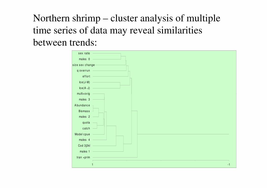
Northern shrimp – cluster analysis of multiple
time series of data may reveal similarities
between trends:
multi+ov ig
Ic e(J-M)
Ic e(A -J)
s ex ra tio
males 0
s iz e s ex c hange
q ov errun
ef f o r t
A bundanc e
B iomas s
quota
c atc h
males 2
Mode l c pue
multi+ov ig
males 3
males 4
Cod 3 j3kl
ma les 1
tran +pr im
-11

Use a correlation matrix from Pearson’s option of cluster analysis
to decide on variables to include in a northern shrimp traffic light
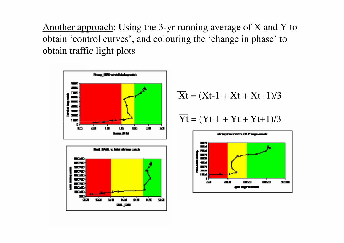
Another approach: Using the 3-yr running average of X and Y to
obtain ‘control curves’, and colouring the ‘change in phase’ to
obtain traffic light plots
Xt = (Xt-1 + Xt + Xt+1)/3
Yt = (Yt-1 + Yt + Yt+1)/3Yt = (Yt-1 + Yt + Yt+1)/3

What indicators to choose from the larger number
available?
Weighting:
One proposition is that two or more indicators derived from the One proposition is that two or more indicators derived from the
same basic data source are likely to be correlated, and perhaps
should be given a fractional weighting related inversely to the
number involved?

Some examples of TL approaches:
Black Sea fisheries

8 different modelling approaches to date have assumed different causes
for Black Sea problems! Six are listed below. They suggest having access
to a wide range of environmental/biological/socio-economic indicators:
1) The ECOPATH model assumes an exotic jellyfish impacts the pelagic fish
food web.
2) Increased nutrient inputs lead to abnormal phytoplankton blooms.
3) Pollution of incoming rivers affected planktonic productivity in the Black
SeaSea
4) Reproductive success of small pelagics is affected more by environment
than spawning stock size
5) A steady state model (ignoring the changing environment) suggests that
stock collapse was mostly due to overfishing
6) Elimination of top predators in the 1970s drove a trophic cascade affecting
all later events.

Pick variables to monitor that do not tie you down to
only one explanation of events in the fishery
�Do not tie yourself to one explanation of what is affecting the
stock until you understand it better!
�If you pick the wrong variables to monitor you may end up in
10 years with 10 yrs of irrelevant data!10 years with 10 yrs of irrelevant data!
�You need to extract the most info from your survey samples.
�You need variables that measure abundance, recruitment and
fishing pressure, but also environmental or ecological change and
socio-economic information.

INDICATOR (SPECIES): INDICATOR OF CONDITIONS BY
HABITAT (RELEVANT ACTIONS)
Environment and
productivity
Planktonic productivity, nutrients, shelf hypoxia
Mugilidae/ Mytilidae/
Venus sp.
Indicator species for uncontaminated coastal
lagoons/inshore areas (Lagoon cleanup)
Sturgeons/shads Good stocks = healthy estuarine/riverine conditions
– (low contaminants; adequate fishery escapement)
Phyllophora weed, turbot,
Rapana, Mullidae, gobies
Oxygenated shallow shelf
Rapana, Mullidae, gobies
Plankton and resident small
pelagic fish
Phyto/zooplankton/jelly predators/small pelagic
eggs and larvae? (surveys)
Migratory pelagics (Bonito,
bluefish, mackerels)
Successful migrations are an indicator of
unimpeded migratory routes
GENERAL ECOSYSTEM
INDICATORS:
Pelagic/demersal ratio; Planktivore/piscivore ratio;
Mean trophic level.
FISHING PRESSURE Mortality rates/ fleet size/ capacity / employment
ECONOMIC ANALYSIS NEEDED!
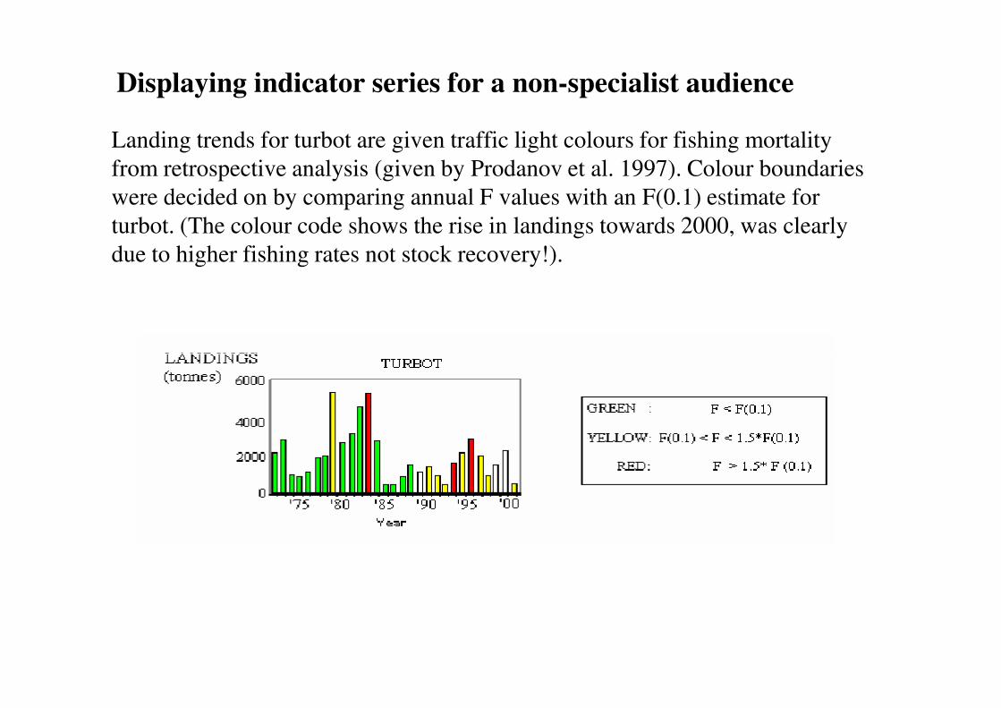
Displaying indicator series for a non-specialist audience
Landing trends for turbot are given traffic light colours for fishing mortality
from retrospective analysis (given by Prodanov et al. 1997). Colour boundaries
were decided on by comparing annual F values with an F(0.1) estimate for
turbot. (The colour code shows the rise in landings towards 2000, was clearly
due to higher fishing rates not stock recovery!).

One obvious approach to indicator development could
be to follow the approach of CITES: look at trends in
landing data, or better, survey data. In the Black Sea,
we have looked at trends in the history of resources by
dividing landing data into 4 phases:
1) A Baseline period: 1967 (when most
statistics began) – 1989.statistics began) – 1989.
2) A Period of Collapse (1989-1992) – when
the Mnemiopsis outbreak became important
3) The Recent period (1992-2002)
4) The last 5 years (1989-2002)
- Indicator values can be referred to the mean
value in 1967-89

Using a 3 colour convention, multiple indicators can be
displayed simultaneously, allowing apparent synchronies and
sequences to be identified – without making a prior
commitment to any particular causal factor.

Gulf of Mexico fisheries

An example from Gulf of Mexico fisheries. Mexican landings
developed rapidly from 1960 in a synchronized fashion (except tunas).
(Overall data ranges divided into 4 quartiles). There is no evidence here
of species interactions – either top-down or bottom-up.
Landings Year Red Grouper Algae and Shrimps Spanish and Oysters Red/ other Mullets Sardines + Sharks Others Mojarras Octopus Tunas
(all species) Sea grasses king mackerels snappers (Mugil spp) other clupeoids (Gerreidae) (Octopus spp)
1940
1941
1942
1943
1944
1945
1946
1947
1948
1949
1950
1951
1952
1953
1954
1955
1956
1957
1958
1959
1960
1961
1962
1963
1964
1965
1966
1967
1968
1969
1970
1971
1972
1973
Z 1974
1975
1976
1977
1978
1979
1980
1981
1982
1983
1984
1985
1986
1987
1988
1989
1990
1991
1992
1993
1994
1995
1996
1997
1998
1999
2000
2001

Looking at the effort data (next) it is clear that species interaction
was secondary to fishing effort impacts. Several different indicators
of fishing effort/investment showed similar trends over time in the
Gulf of Mexico fishery:
Time Fishing effort Fishing effort Fishing effort Financial support
(yr) (Large scale) (small scale) (finfish) (Millions of pesos)
1978
1979
1980
1981
1982
19831983
1984
1985
1986
1987
1988
1989
1990
1991
1992
1993
1994
1995
1996
1997
1998
1999

North Atlantic and Mediterranean
fisheries

In the North Atlantic invertebrate landings have
increased following declines in finfish stocks - an
ecological interaction or a shift in industry
priorities?
Between different finfish species, ecosystem Between different finfish species, ecosystem
interraction seems a less tenable hypothesis than
the ‘whole-system impact’ of industrial fishing
plus climate change/a regime shift?


In the Mediterrean and Black Sea, there was an increase in
production in the 70’s, but many species production
declined significantly in the 1990’s:

From cluster analysis of the GRUND data set, we can recognize
different biogical assemblages made of species that vary together. Even
if information on their interrelationships is scarce, species in the same
‘cluster’ form a common indicator.

Gulf of St Lawrence snow crab

WE CAN USE THE TL APPROACH ON SIZE AND AGE DATA:
The stages (below, left) of the snow crab (Chionoecetes opilio) are
equivalent to year classes. Their abundance in trawl surveys shows a
clear cycle over time: good or poor year classes remain visible as
diagonal strips of colour. Note: A good adult yc (compopsc129)
coincides with poor recruitment of very small crabs (Pub Females).
(This might not be a SRR – C. opilio is a cannibalistic species!).
RecruitmentRecruitment88 89 90 91 92 93 94 95 96 97 98 99 00 01 02 03
Pub Female 2 2 2 1 0 0 1 2 3 2 2 2 1 0 1
PrimFemale 2 2 3 2 1 0 0 0 2 2 2 2 2 1 0
Mat Fem 1 2 3 2 2 1 1 0 1 1 2 1 2 2 1
Instar VIII 3 1 1 0 0 1 1 2 3 3 3 2 1 0 1
R3 1 2 3 2 1 0 0 0 1 2 2 2 3 2 1
R2 0 1 3 2 2 1 1 0 0 1 2 2 3 3 2
R1 0 1 2 2 3 3 2 1 1 1 1 1 1 2 2
Com Popsc12 0 0 1 1 2 3 2 2 1 1 1 1 1 2 2

Fig. 12. Recruitment indicators can be lagged so that good
and poor cohorts passing through the population show up as
vertical colour bands: i.e., year class size is determined early
on – by cannibalism? This plot also helps provide a rough
forecast of future yields, and shows decadal cycles?
Recruitment88 89 90 91 92 93 94 95 96 97 98 99 00 01 02 03 04 05 06 07 08 09 10 11 12 13 14 15 16 17
Pub Female +14Pub Female +14 2 2 2 1 0 0 1 2 3 2 2 2 1 0 1
PrimFemale +13 2 2 3 2 1 0 0 0 2 2 2 2 2 1 0
Mat Fem +12 1 2 3 2 2 1 1 0 1 1 2 1 2 2 1
Instar VIII +5 3 1 1 0 0 1 1 2 3 3 3 2 1 0 1
R3 +3 1 2 3 2 1 0 0 0 1 2 2 2 3 2 1
R2 +2 0 1 3 2 2 1 1 0 0 1 2 2 3 3 2
R1 +1 0 1 2 2 3 3 2 1 1 1 1 1 1 2 2
Com Popsc12 0 0 1 1 2 3 2 2 1 1 1 1 1 2 2
average 0 0 1 1 2 3 2 1 1 0 1 1 1 2 2 2 2 1 1 0 1 1 2 2 2 2 2 1 0 1

Frequency of ice occurrence in March, from sea ice charts over 1972-
1990. More recently there has been a warming trend and melting of
Arctic Ocean/Greenland ice, and southerly flow of cold low salinity
water down to the Grand Banks - i.e., the water has been colder off
Eastern Canada – not good for cod; better for shrimp and snow crab!.

Davis Strait Pink Shrimp : a
changing ecosystemchanging ecosystem
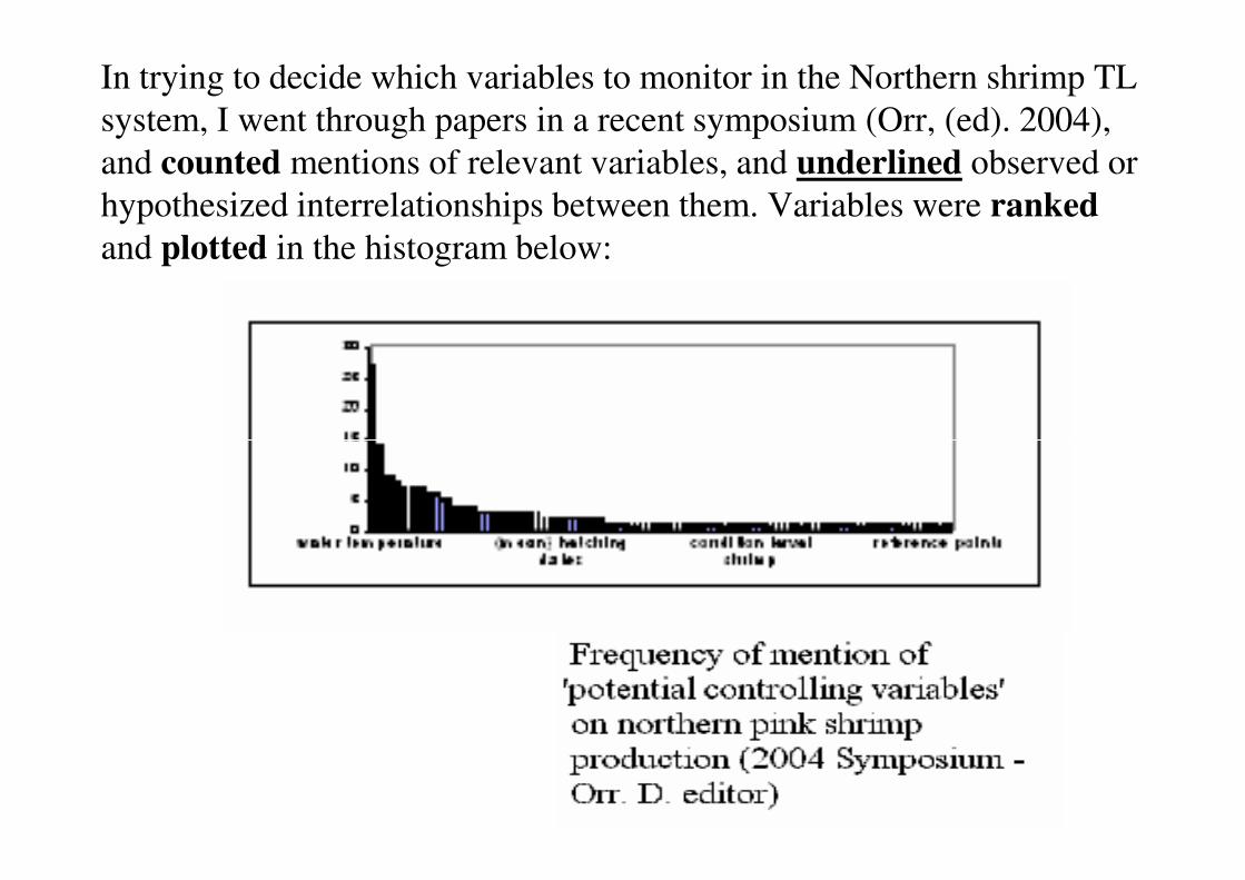
In trying to decide which variables to monitor in the Northern shrimp TL
system, I went through papers in a recent symposium (Orr, (ed). 2004),
and counted mentions of relevant variables, and underlined observed or
hypothesized interrelationships between them. Variables were ranked
and plotted in the histogram below:


YC strength can be established roughly without cohort
analysis by lagging numbers at age, then averaging
numbers in each cohort separately (Nfld shrimp/cod)
relative cohort strength in year - cod/male shrimp
0.00
2.00
4.00
6.00
8.00
10.00
12.00
14.00
16.00
1970 1980 1990 2000 2010
year
rela
tive
str
en
gth
cohort relative strength
(cod?)
cohort relative strength
(male shrimp)

Problems with time lags: Comparing shrimp catch/biomass and bottom temperature
time series for different lags before incorporating an environmental (driving) variable
into a traffic light series (-2 yr lags seemed best for shrimp predator biomasses; -6 year
lags for environmental data (Pandalus borealis is a protandric hermaphrodite -
harvested as females at age 6+).

A simple ecosystem model incorporating northern shrimp:
showing one way of setting colour boundaries in the TL

Monitoring the fishery and
displaying results

The Amoeba method is well suited to displaying the output
from questionnaires – segments that fall in the ‘red’ area are in
serious need of improvement (after Pajak 2000).
Summary of sustainability indicators from 3 sectors for three levels of indicators have
been set: Those entering the ‘Red’ zone are ‘unsafe’; the ‘Yellow’ category from 35 –
70% is ‘uncertain’ – i.e., unsatisfactory but not dangerous conditions prevail inside
the yellow circle.

Using the TL approach in
management

The TL approach can be used in a conventional
fisheries control law (�the allowable F values
decline as the biomass declines)

Fishery managers need understandable
indicator values to help them in decision
making – a suggested mechanism:
• The interface between science advice and
management decision-making should be clear cut. management decision-making should be clear cut.
• A Consideration Matrix is one option suggested
by the FRCC for an interface between scientists
and managers (see next slide)

A simple approach based on annual science evaluations requires
appropriate actions by managers when fishery indicators turn ‘red’,
‘yellow’ or ‘green’. ‘Science’ puts the fishery in one of 9 boxes each
year, and management agrees to implement the management
recommendation within that box.

IN SUMMARY:
The traffic light approach is a flexible way of
summarizing data of concern to fisheries
managers, is easily understandable by non-
technical personnel, and may also be useful for
hypothesis formulation in science, and planning hypothesis formulation in science, and planning
further multivariate scientific investigations.
THE END
