A TRIDENT SCHOLARPROJECT REPORT

NO. 261

"Design, Construction, and Analysis of a Flat Heat Pipe"

UNITED STATES NAVAL ACADEMY

ANNAPOLIS, MARYLAND

IThs document has been approved for publicrelease and sale; its distribution is unlimited.

DTIC QUA INSPECTED 3 20000424 149 U.JIqA-1531-2

REPORT DOCUMENTATION PAGE Form Approved7 OMB No. 074-0188

Pubic reporting burden for this collection of information is estimated to average 1 hour per response, including g the time for reviewing instructions, searching existing datasources, gathenng and maintaining the data needed, and completing and reviewing the collection of information. Send comments regarding this burden estimate or any otheraspect of tne coliection of information, incuding suggestions for reducing this burden to Washington Headquarters Services, Directorate for Information Operations and Reports,t215 Jefferson Davis Hignway, Suite 1204, Arlington. VA 22202-4302. and to the Office of Management and Budget. Paperwork Reduction Project (0704-0188), Washington, DC20503.

1. AGENCY USE ONLY (Leave blank) 2. REPORT DATE 3. REPORT TYPE AND DATE COVERED15 May 1999

4. TITLE AND SUBTITLE 5. FUNDING NUMBERSDesign, construction, and analysis of a flat heat pipe

6. AUTHOR(S)Boughey, Britt W.

7. PERFORMING ORGANIZATION NAME(S) AND ADDRESS(ES) 8. PERFORMING ORGANIZATION REPORT NUMBER

U.S. Naval Academy USNA Trident Scholar project reportAnnapolis, MD no. 261 (1999)

9. SPONSORING/MONITORING AGENCY NAME(S) AND ADDRESS(ES) 10. SPONSORINGIMONITORING AGENCY REPORT NUMBER

11. SUPPLEMENTARY NOTESAccepted by the U.S. Trident Scholar Committee

12a. DISTRIBUTIONIAVAILABILITY STATEMENT 12b. DISTRIBUTION CODEThis document has been approved for public release; its distributionis UNLIMITED.

13. ABSTRACT: Thermophotovoltaic (TPV) energy conversion utilizes photons from a thermal radiator to convert photonicenergy to electrical energy. Due to the nature of the system, the thermal radiator must emit uniform radiation andtherefore maintain a uniform temperature profile in order to achieve maximum efficiency. Heat pipe technology caneffectively meet the demand for an isothermal emitter as it utilizes near isobaric phase changes to transfer heat ata uniform temperature. In this project, heat pipes are explored for use in TPV energy conversion systems. A flat heatpipe offers many advantages over the conventional cylindrical design. These include increased surface area to volumeratio in order to maximize power density, as well as the ability to stack or layer the system with photovoltaic 4PV)cells on both sides of the flat heat pipe to utilize available energy. Not only do flat heat pipes present uniqueengineering demands inherent in their operation to counteract pressure differences across their vessel walls, butthey are also difficult to construct. To date, only limited analyses of their thermal characteristics have been donefor use in performance predictions. Therefore, it is necessary to conduct analyses to enable consideration of heatpipes for implementation into TPV systems. This report details the design and construction of a flat heat pipeanalysed both in symmetric and asymmetric heating conditions, involving a low temperature version of future emitterdesigns due to safety considerations. Water was used as a working fluid instead of the liquid metal required toachieve the temperatures of a functional emitter. Despite this difference in working fluid, the data presented isvaluable to both TPV and heat pipe research.

14. SUBJECT TERMS 15. NUMBER OF PAGESheat pipe, emitter, isothermal, thermophotovoltaic

16. PRICE CODE

17. SECURITY CLASSIFICATION 18. SECURITY CLASSIFICATION 19. SECURITY CLASSIFICATION 20. LIMITATION OF ABSTRACTOF REPORT OF THIS PAGE OF ABSTRACT

NSN 7540.01-280-5500 Standard Form 298(Rev.2.89) Prescribed by ANSI Std. Z39-18

298-102

U.S.N.A. - Trident Scholar project, report; no. 261 (1999)

"Design, Construction, and Analysis of a Flat Heat Pipe"

by

Midshipman Britt W. Boughey, Class of 1999United States Naval Academy

Annapolis, Maryland

Certification of Advisors' Approval

Professor Keith W. LindlerDepartment of Naval Architecture, Ocean and Marine Engineering

(signature)

(date)

Associate Professor Martin R. CerzaDepartment of Naval Archie e, Oean and Marine Engineering

(signature) -( --

(date)

Acceptance for the Trident Scholar Committee

Professor Joyce E. ShadeChair, Trident Scholar Committee

USNA-1531-2

ABSTRACT

Thermophotovoltaic (TPV) energy conversion utilizes photons from a thermalradiator to convert photonic energy to electrical energy. Due to the nature of the system, thethermal radiator must emit uniform radiation and therefore maintain a uniform temperatureprofile in order to achieve maximum efficiency. Heat pipe technology can effectively meetthe demand for an isothermal emitter as it utilizes near isobaric phase changes to transfer heatat a uniform temperature. In this project, heat pipes are explored for use in TPV energyconversion systems. A flat heat pipe offers many advantages over the conventionalcylindrical design. These include increased surface area to volume ratio in order tomaximize power density, as well as the ability to stack or layer the system with photovoltaic(PV) cells on both sides of the flat heat pipe to utilize available energy. Not only do flat heatpipes present unique engineering demands inherent in their operation to counteract pressuredifferences across their vessel walls, but they are also difficult to construct. To date, onlylimited analyses of their thermal characteristics have been done for use in performnancepredictions. Therefore, it is necessary to conduct analyses to enable consideration of heatpipes for implementation into TPV systems. This report details the design and constructionof a flat heat pipe analysed both in symmetric and asymmetric heating conditions, involvinga low temperature version of future emitter designs due to safety considerations. Water wasused as a working fluid instead of the liquid metal required to achieve the temperatures ofa functional emitter. Despite this difference in working fluid, the data presented is valuableto both TPV and heat pipe research.

KEYWORDS: heat pipe, emitter, isothermal, thermophotovoltaic

2

TABLE OF CONTENTS

ABSTRACT 1TABLE OF CONTENTS 2LIST OF FIGURES 4NOMENCLATURE 6

1.0 INTRODUCTION 9

1.1 OBJECTIVES1.2 METHODOLOGY

2.0 THERMOPHOTOVOLTAICS BACKGROUND 11

2.1 PHOTOVOLTAIC PHYSICS2.2 TPV EFFICIENCY

3.0 HEAT PIPE INTRODUCTION 15

3.1 STEADY-STATE LIMITS3.2 WICK DESIGNS

4.0 FLAT HEAT PIPE PROPERTIES 22

4.1 FLAT HEAT PIPE HEATING LIMITS4.2 FLAT HEAT PIPE STRUCTURAL CONSIDERATIONS

5.0 USNA FLAT HEAT PIPE DESIGN 26

5.1 CALCULATED LIMITS5.2 HEAT TRANSFER CALCULATIONS

6.0 SUBSCALE FLAT HEAT PIPE 32

6.1 SUBSCALE HEAT PIPE CONSTRUCTION

6.2 SU1BSCALE HEAT PIPE TESTING

6.3 SUBSCALE HEAT PIPE TESTING RESULTS6.4 IMPLICATIONS FOR FULLSCALE HEAT PIPE

7.0 FULLSCALE HEAT PIPE CONSTRUCTION 37

7.1. FULLSCALE HEAT PIPE CONSTRUCTION DETAILS

8.0 EXPERIMENTAL SETUP AND PROCEDURE 40

8.1 EXPERIMENTAL SETUP8.2 EXPERIMENTAL PROCEDURE

3

9.0 DATA ANALYSIS 50

9.1 HORIZONTAL TESTS! HEAT PIPE VERIFICATION9.2 ORIENTATION EFFECTS9.3 CHARGING EFFECTS9.4 START-UP TRANSIENTS9.5 ASYMMETRIC TESTING9.6 VARIABLE CONDUCTANCE EFFECTS

10.0 CONCLUSIONS AND MODELLING 65

10. 1 GOALS MET10.2 RECOMMENDATIONS

11.0 REFERENCES 67

APPENDICES 68

APPENDIX I - CAPILLARY LIMIT DERIVATIONSAPPENDIX 2 - BOILING LIMIT DERIVATIONAPPENDIX 3 - SONIC LIMIT DERIVATIONAPPENDIX 4 - DEFLECTION DERIVATIONS AND SPREADSHEETAPPENDIX 5 - MATHCAD MODELLING OF FIN VS HEAT PIPE

ACKNOWLEDGMENTS 99

4

LIST OF FIGURES

PAGE

FIGURE 1. BASIC TPV SYSTEM 11

FIGURE 2. PLANCK'S LAW 12FIGURE 3. AXIAL FLOW TPV- HEAT PIPE SYSTEM 14FIGURE 4. BASIC HEAT PIPE 15FIGURE 5. GAS LOADING EFFECTS 16FIGURE 6. HEATING LIMITS 18FIGURE 7. WETTING ANGLE 19FIGURE 8. SUBCALE HEAT PIPE EXTERIOR 28FIGURE 9. SUBSCALE HEAT PIPE DETAIL 29FIGURE 10. FULLSCALE FLAT HEAT PIPE EXTERIOR 30FIGURE 11. FULLSCALE FLAT HEAT PIPE DETAIL 31FIGURE 12. CHARGING ASSEMBLY 34FIGURE 13. SUBSCALE HEAT PIPE PHOTO 35FIGURE 14. PHOTO OF INFRARED CAMERA 36FIGURE 15. CLOSE-UP PHOTO OF VESSEL 38

FIGURE 16. COMPLETED HALVES 38FIGURE 17. • SCREEN SIDE VIEW WITH BENT SIDE 39FIGURE 18. SHEET WITH PINS 39FIGURE 19. PHOTO OF SYMMETRIC HEATER MOUNTING 41FIGURE 20. PHOTO OF ASYMMETRIC HEATER MOUNTING 41FIGURE 21. PHOTO OF HEAT PIPE END FITTING WITH PRESSURE TRANSDUCER 42FIGURE 22. PHOTO OF HEAT PIPE END FITTING WITH ANALOG PRESSURE 43

GAUGE

FIGURE 23. PHOTO OF HEAT PIPE TEST STAND 44FIGURE 24. PHOTO OF TEST STAND CLAMP MOUNTED TO HEAT PIPE 45

FIGURE 25. THERMOCOUPLE PLACEMENT BY NUMBERS 46FIGURE 26. PHOTO OF THERMOCOUPLES MOUNTED 47FIGURE 27. PHOTO OF DATA ACQUISITION SETUP 47FIGURE 28. HEAT PIPE TESTING ORIENTATIONS 49

FIGURE 29. HEAT TRANFER REJECTION MODES FOR HEAT INPUT 51FIGURE 30. STANDARD FIN VS IDEAL HEAT PIPE FIN AND ACTUAL HEAT PIPE 52

(400 W STEADY-STATE, HORIZONTAL)

FIGURE 31. IR PHOTO OF HORIZONTAL HEAT PIPE, 800W, 125% CHARGE 53FIGURE 32. NEAR ISOTHERMAL CASE TEMPERATURE VS TIME, 53

HORIZONTAL, 600W, 100% CHARGE

FIGURE 33. HEAT PIPE TEMPERATURE VS. ANGLE, 400W 55FIGURE 34. IR PHOTOGRAPH, VERTICAL (5), 600W 56FIGURE 35. VERTICAL GRADIENT, 400W, 125% CHARGE 56FIGURE 36. TEMPERATURE VS TIME, 400W, 125% CHARGE 57FIGURE 37. TEMPERATURE VS TIME, 400W, 100% CHARGE 58FIGURE 38. TEMPERATURE VS TIME, 400W, 75% CHARGE 58

5

FIGURE 39. VARYING CHARGES TEMPERATURE Vs. TIME, 400W, HORIZONTAL 59FIGURE 40. THEORETICAL HEAT PIPE START-UP 60FIGURE 41. TEMPERATURE VS TIME FOR 100% CHARGE, 400-800W, 61

HORIZONTAL

FIGURE 42. ASYMMETRIC, HORIZONTAL, 200W 62FIGURE 43. ASYMMETRIC, HORIZONTAL, 400W 62FIGURE 44. ASYMMETRIC, HORIZONTAL 600W 63FIGURE 45. ASYMMETRIC, INCLINED, 400W 63FIGURE 46. ASYMMETRIC, INCLINED, 400W 64

6

NOMENCLATURE

General Terms

A area (usually cross-sectional) (in2 )a acceleration (m/s 2)C constant value in an equationc integration constantF function of, or friction coefficientf function of, or frictiona acceleration due to gravity (m/s2)Gr Grashof numberH height (m)h heat transfer convection coefficient [W/(m K)]K permeability (M2)k thermal conductivity [W/(m K)]L length (m)

length of subsection (m)In mass (kg), term in fin equationrh mass flow rate (kg/s)Ma Mach numberN Screen mesh numbern number of repeated elementsNu Nusselt numberP pressure (N/m 2), perimeter (m)Pr Prandtl numberQ heat rate (W)R gas constant for given vapor [kJ/(kg K)]r radius (m), radius of curvature (m)Ra Rayleigh numberRe Reynolds numbers spacer distance (in)T temperature (K)t time (s), thickness (in)U overall heat transfer coefficient [W/(m 2 K)]V volume (M 3), velocity (m/s)v specific volume (m 3/kg)W width (m)We Weber numberx cartesian coordinatey cartesian coordinatez cartesian coordinate

7

Specific Terms

Al cross-sectional area of liquid flow path (M2)

A, total wetted surface area of wick (M2)A,. vapor flow cross-sectional area (M2)A. area in x-direction (m2)C, first radiation constant (3.7415 x 10-16 W M 2), first constant of integrationC2 second radiation constant (1.4388 x 10-2 m K), second constant of integrationco speed of sound evaluated at evaporator end cap temperature (m/s)Dv diameter of vapor core (m)Eb total emissive power (W/m2)EbX blackbody emissive power at absolute temperature T for a single wavelength

(W/m3)F, liquid frictional coefficientF, frictional coefficient for vaporg acceleration due to gravity (mis 2)hfg latent heat of vaporization (kJ/kg)K' ratio of specific heatsk, thermal conductivity of working fluid in liquid phase [W/(m K)]keff effective thermal conductivity of the wick [W/(m K)]ks thermal conductivity of wick material [W/(m K)]k, thermal conductivity of vapor [W/(m K)]kt thermal conductivity of vessel wall material [W/(m K)]Le Evaporator length (m)Leor effective fluid return length (m)Lt total length (m)

liquid mass flow rate (kg/s)vapor mass flow rate (kg/s)

PO pressure at evaporator end (N/m 2)

Qb maximum heat rate at boiling limit (W)Qent maximum heat rate at entrainment limit (W)

Q, maximum heat rate at sonic limit (W)Qis maximum heat rate at viscous limit (W)QL heat transport capability (W m)

4e maximum heat flux into evaporator section (W/m 2)

Rh.W hydraulic radius of wick surface pore (m)R, inner radius of pipe wall (m)R,, vapor space radius (m)VP,I liquid velocity through wick screen pores (m/s)Tamb temperature of ambient environment (K)Th temperature of hot (radiating) body (K)Tlocal local temperature (K)TS steady-state temperature (K)t, vessel wall thickness (m)

8

wick thickness (m)APcap.max maximum capillary pumping pressure (N/m2)Ap, pressure drop due to gravitational force (N/m2)Ap1 liquid pressure drop (N/m2)

Ap. pressure drop in vapor (N/m2)ATcrit Wall Superheat temperature difference (K)

Greek Symbols

8V thickness of vapor flow cross-section (assume uniform for entire heat pipe) (m)13 coefficient of thermal expansion (1/K)E surface emissivity. wavelength (m)

Xmarx wavelength at which an ideal radiator emits maximum amount of energy•1 liquid viscosity(N s/m 2)P0 vapor density evaluated at evaporator end cap temperature (kg/m 3)PI density of liquid (kg/rM3)P, vapor density (km 3)a liquid surface tension (N/m), Stefan-Boltzmann constant [5.67 x 10-8 W/(m2 K4)]

angle of heat pipe from horizontal (degrees)(P wick porosity

9

1.0 INTRODUCTION

This project report entails the design, construction, and both the theoretical andexperimental thermal performance investigation of a flat heat pipe using water as theworking fluid. The project's findings will help determine the viability of implementing flatheat pipes into thermophotovoltaic energy conversion systems.

1.1 OBJECTIVES

The flat heat pipe was designed to meet the following criteria (as determined by boththe sponsors of the project and the research team):

1. Design and construct the heat pipe entirely out of Monel 400.2. Exhibit two-dimensional heat transfer behavior.3. Feature ultimate dimensions of 4 feet long (1.22 mn) by 1 foot wide (30.48 cm) byV/2 inch-thick (1.27 cm).4. Maintain an operating temperature of up to 212'F (I100 0 C).5. Possess a means of internal support for structural rigidity without sacrificing two-dimensional flow capabilities.6. Operate without the presence of any noncondensable gases, such as air, inside ofthe heat pipe (gas loading).

The following experimental and theoretical goals were set:

1. Monitor the condenser region temperature profile as closely as possible, viathermocouples and infrared video camera.2. Test asymmetric heating conditions and different heat inputs.3. Test performance at different heat inputs, fluid charges, and varying inclinationangles.4. Modify important heat pipe equations for flat geometry.5. Model experimental and theoretical heat pipe performance against a conventionalfin of the same dimensions.6. Analyze experimental data to determine overall performance and feasibility offlat heat pipes for a TPV energy conversion system.

1.2 METHODOLOGY

The design, experimental, and theoretical goals were met in the following manner:

Step 1: Research and Design

A literature search was conducted to determine the mechanisms of heat transfer inheat pipes and how they might differ in a flat heat pipe from a cylindrical heat pipe. Severalexperts in the field, with specialties ranging from design and theoretical analysis to

10

fabrication, were consulted and their recommendations considered. Suppliers of thenecessary materials were located. The final design was completed incorporating all of theabove research.

Step 2: Construction and Testing

A subscale model of the final design was submitted to Technical Support Department(TSD) at USNA for construction to allow fabrication difficulties to be solved beforeattempting the final design. Instrument calibration and basic heat pipe operationalprocedures, such as fluid charging, were perfected with this model. The subscale model alsoserved to provide insight that was incorporated in revisions for the fuliscale model. Finally,the fullscale heat pipe was constructed, tested, and analyzed under the test conditions.

Step 3: Analysis

The raw data from the experiments were collected and reduced. The infrared cameradata was used to aid in explaining the purely quantitative thermocouple data as well asprovide visual understanding of heat pipe phenomena. The temperatures of regions at thesame distance axially from the heater end were compared to other equidistant regions andanalyzed for thermal performance assessment at varying heat inputs, fluid charge, and anglesof inclination. A traditional fin, with the same dimensions as the fuliscale heat pipe, wasmodelled against the heat pipe's performance. This demonstrated the heat pipe's ability totransfer large quantities of heat with a near isothermal profile; a quality not found in atraditional fin.

11

2.0 THERMOPHOTOVOLTAICS (TPV) BACKGROUND

TPV energy conversion is a phenomenon by which infrared thermal radiation isconverted into electrical power with no moving parts. The basic components of the systeminclude the thermal radiator and a semiconductor diode (thermophotovoltaic cell) thatconverts thermal radiation into electrical power. Only photons with energy greater than thebandgap, or threshold energy of the TPV cell, can be converted into electrical energy. Theradiation not converted either creates heat in the cell or is recycled to the radiator viareflection if such a system (known as spectral control) exists. The bandgap energy isdetermined by the TPV cell material and is not a variable parameter (Erickson, 1997). Fora schematic of the basic TPV system, see Figure 1.

Spectral Control TPV Cell

-- • +l P N

+j-N>

Radiation

- II

Figure 1. Basic Thermophotovoltaic Energy Conversion System

Figure 2 shows the emissive power over differing wavelengths for theoreticalblackbodies at different temperatures. A blackbody, or ideal radiator, is an object that emitsthe maximum possible amount of radiation at any given wavelength. The emissive poweris a function of only the temperature of the emitter. The emissive power for a singlewavelength is given by Planck's law in equation 2.1:

(2.1)

C,Eb " = X5(eC /2 T _ 1)

From Figure 2 it is apparent that increasing temperature will increase the emissivepower of the blackbody for a given wavelength. The wavelength at which the emissive

12

power is maximized (which corresponds to the peak of the curve for each temperature inFigure 2) is found by Wien's displacement law given in equation 2.2:

(2.2)

2.898x10-'m K2 max= T

Monochromatic Emissive Power

1E+10 - 12

1E+08

1E+06-E _____ ____

>1 E+04- 1000,

SE+02IL

lu 1E+00 A I_ 1_ 7-

E 1 E-02 -Ll1E-04 / 2 / L l'l0.1 1 10 100

Wavelength, microns

Figure 2. Planck's Law

The total emissive power of a blackbody at a given temperature is the area underneaththe curve corresponding to the given temperature in Figure 2. This is represented in equation2.3, the Stefan-Boltzmann law (where u is the Stefan-Boltzmann constant):

(2.3)Eb(T) = aT 4

Since power is proportional to temperature to the fourth power, small changes in thetemperature of an emitter can have great effects on emissive power.

2.1 PHOTOVOLTAIC PHYSICS

The physical mechanism within the TPV cells that governs the conversion of photonsinto electrical energy is the photoelectric effect, the same principle which standardphotovoltaic (PV) cells (also known as solar cells) utilize. The active layer of these cells is

13

constructed of a semiconductor material with a P-N (Positive-Negative) junction. Thematerial used to produce the active cell layers determines the bandgap energy, or the energynecessary to dislodge an electron from the material's outermost electron shell. As photonsfrom the thermal radiator travel into the TPV cell, they travel through the "window" and areabsorbed by the semiconductor. If the energy of the photon striking the semiconductor issufficient, the semiconductor will eject an electron from its outer shell, leaving a "hole."If not, it will cause the temperature of the material to rise. If the difference in energybetween the "hole" and the ejected electron is greater than the bandgap energy of thematerial, the pair (electron and hole) will cross the voltage barrier of the cell. When thischarge-carrying pair moves towards similarly charged regions and moves away from layersof unlike charge, it becomes an electrical current, or usable electrical energy. The amountof energy available to be converted into electricity by the photoelectric effect is determinedby Planck's law (see equation 2.1). Only photons that have energy (emissive power) greaterthan bandgap energy can produce an electron-hole pair (and therefore produce electricity)(Coutts and Fitzgerald, 1998).

As established, PV (and therefore TPV) cells can only convert certain wavelengthsof electromagnetic radiation into usable energy. Therefore, the system efficiency is afunction of the wavelengths emitted by the thermal radiator. As shown in Figure 2,wavelength is a function of temperature. Therefore, TPV cell efficiency is a function ofradiator temperature. Methods do exist of reflecting back emitted wavelengths that cannotbe utilized by the TPV cells for reabsorption into the emitter. This is known as spectralcontrol. It ensures that the TPV cells receive only usable wavelengths ofphotons, and resultsin higher energy conversion efficiencies. However, spectral controls cannot moderate theamounts of radiation that come from different regions of the emitter (corresponding tolocations on the emitter of different temperature) (Borowsky and Dziendziel, 1996).

2.2 TPV CELL EFFICIENCY

TPV and PV cells must be linked together in series to produce an appreciable voltage,as the voltage output of a single cell is small. Since the cells are in series, the same amountof current must flow through each cell. Experience has shown that if one cell in a series ofTPV cells receives fewer photons above bandgap energy than the other cells (due to a lowtemperature region on the emitter) then the performance of the entire series of cells isdowngraded (Lindler, 1999). Therefore, the emitter must exist at a uniform temperature formaximum efficiency. This presents a substantial problem for emitter design in TPV energyconversion systems. Combustion processes can have inherent non-isothermal profiles andtherefore can not operate TPV cells at a high efficiency. However, heat pipes provide ameans of heat transfer that maintains a nearly isothermal surface and could serve as emittersin TPV generators. Figure 3 shows just such a system. Heat pipes are heated axially viafossil fuel combustion. Alternating heat pipes and TPV cells results in a large surface areato volume ratio.

14

//2/4 /• TPV cells

Heat Pipe

Radiator / Fin /

Combustion Chamber

Figure 3. USNA TPV axial flow concept

15

3.0 HEAT PIPE INTRODUCTION

Heat pipes have existed for decades and stem from a simple principle: vaporevaporates and condenses at a uniform temperature for a given pressure. A heat pipe consistsof a hermetically sealed vessel, a working fluid, and a wick that lines the vessel. Theworking fluid is vaporized (by an external heat source) and leaves the wick as a vapor. Thevapor travels from the evaporator end to the condenser end of the heat pipe and condensesin the wick, releasing heat. Due to the change in phase of the working fluid, the heat isdelivered to the condenser end at an almost isothermal profile. The fluid returns to theevaporator end from the condenser end via the capillary pumping action of the wick. Figure4 shows the basic configuration of a cylindrical heat pipe.

~LHeat in Vessel Heat out .. $

4 iq nid Retui 11-U Vapor Flow~~- Wick I

Evaporator End Adiabatic Region Condenser End

Figure 4. Basic Heat Pipe Configuration

Constructing and operating a heat pipe is an involved process, with many limitationsto be considered. First, the fluid and vessel must be of high purity. If the fluid is not pure,then its heat transfer properties may fluctuate from the expected standard. Impure fluid canalso deposit undesirable substances in the heat pipe vessel and vapor space, such asnoncondensable gases. Undesired gases in the vapor space serve to effectively blanket thecondenser area and raise the temperature of the heat pipe in the areas removed from the gaswhile the areas where the gas is located remain colder than the rest of the heat pipe. Thiseffect, called gas loading, differs for varying heat inputs. Figure 5 serves to illustrate thiseffect (Ashcroft, 1996).

If the vessel is impure, then the working fluid may possibly erode parts of the vessel(e.g. impurities) (Ashcroft, 1996). The vessel material must also handle large compressiveand tensile forces (Peterson, 1994).

16

>Non-functioning condenser area

Air Low Power

~I~ir Medium Power

SEHigh Power

Evaporator Condenser

Figure 5. Gas Loading Effect

3.1 STEADY-STATE LIMITS

The heat pipe has many different operating limits for given input heating powers andoperating temperatures. When too much heat is applied the working fluid is superheated andbubble formation occurs in the wick, which then dries out and interrupts heat transfer. Thisis known as the boiling limit and is represented by equation 3.1 (for cylindrical heat pipes)(Faghri, 1995):

(3.1)

2 7rLekeffA TQb : In(•-

The viscous limit primarily exists in heat pipes that have startup conditions inwhich the working fluid is solidified (such as in high temperature liquid metal heat pipes).It is possible for the working fluid to liquefy and be vaporized from the evaporator regionand condense in the condenser region without sufficiently heating the frozen fluid in thecondenser region to allow flow back into the evaporator region. The evaporator will then dryout and the heat pipe will not reach normal operating conditions. In general, the viscouslimit can be reached when a heat pipe is operating at temperatures below its normal operatingrange, when viscous forces dominate the vapor flow and vapor pressure in the condenser endis reduced to zero, limiting the heat transport capabilities of the heat pipe. The viscous limitis expressed by equation 3.2 ( for cylindrical heat pipes) (Peterson, 1994):

17

(3.2)Dhfo POJ

Q ," - 6 4 /ILeff

At low vapor densities (and hence, low temperatures), the vapor velocity must behigh to transfer the necessary heat. For a constant area duct, the vapor velocity can notexceed the local sonic velocity. Therefore, problems such as dryout, shock, and largetemperature fluctuations result. The sonic limit is related as follows in equation 3.3 (Dunnand Reay, 1976):

(3.3)

Q PocohfgAv

-vF2(K'+ 1)

In certain wick designs, it is also possible for the vapor that is traveling to thecondenser end to capture, or entrain, the returning liquid and cause dryout. This limit,known as the entrainment limit, is expressed as (Chi, 1976):

(3.4)

Q e n1 = A vh j ( ; o 1/2"2h,R,

The most important limit for design considerations, the capillary limit, is met whenthe vapor and liquid pressure drops exceed the maximum capillary head that the wickproduces. This maximum head is related to the wick's effective pore size. The capillarylimit occurs when the pumping ability of a given wicking material to provide the circulationfor the working medium can no longer return fluid as fast as the evaporator vaporizes it.This limit will cause the evaporator end to dry out, resulting in damage to the vessel andwick. The capillary limit is the highest heat rate that most heat pipes can operate at to achieveminimum design operating temperature and is therefore usually the only limit given for heatpipes. See Figure 6 for the relations of temperature and heat rate to heating limits for aconventional cylindrical heat pipe. Equation 3.5, the equation for the capillary limit for acylindrical heat pipe, neglecting the pressure drops due to evaporation and condensation, is(Faghri, 1995):

(3.5)

( QL)•capmax - Apcp'max- ApgF i F ,ic

(QL)cap,max. is the heat transport capability (W mn), F, is the liquid friction loss coefficient, and

18

F, is the vapor friction loss coefficient. Equations 3.6 through 3.10 further define theelements of the capillary limit equation (equation 3.5).

(3.6)Apcapmax = (2 0)/reff

Apcapmax is the maximum capillary pumping head

(3.7)Apcap,max Ž Ap1 + Ap, + Apg, where

(3.8)

lbeff 'hi

Ap, is the pressure drop in liquid(3.9)

Ap, = , veff rh,pvk,,A,

Ap, is the pressure drop in the vapor(3.10)

Apg = p1 gLt sin q

Apg is the pressure drop due to gravity and sin 4 = angle of inclination from horizontal

Capillary

Entrainmen

SSoni

SBoiling

Temperature

Figure 6. Heating Limits

19

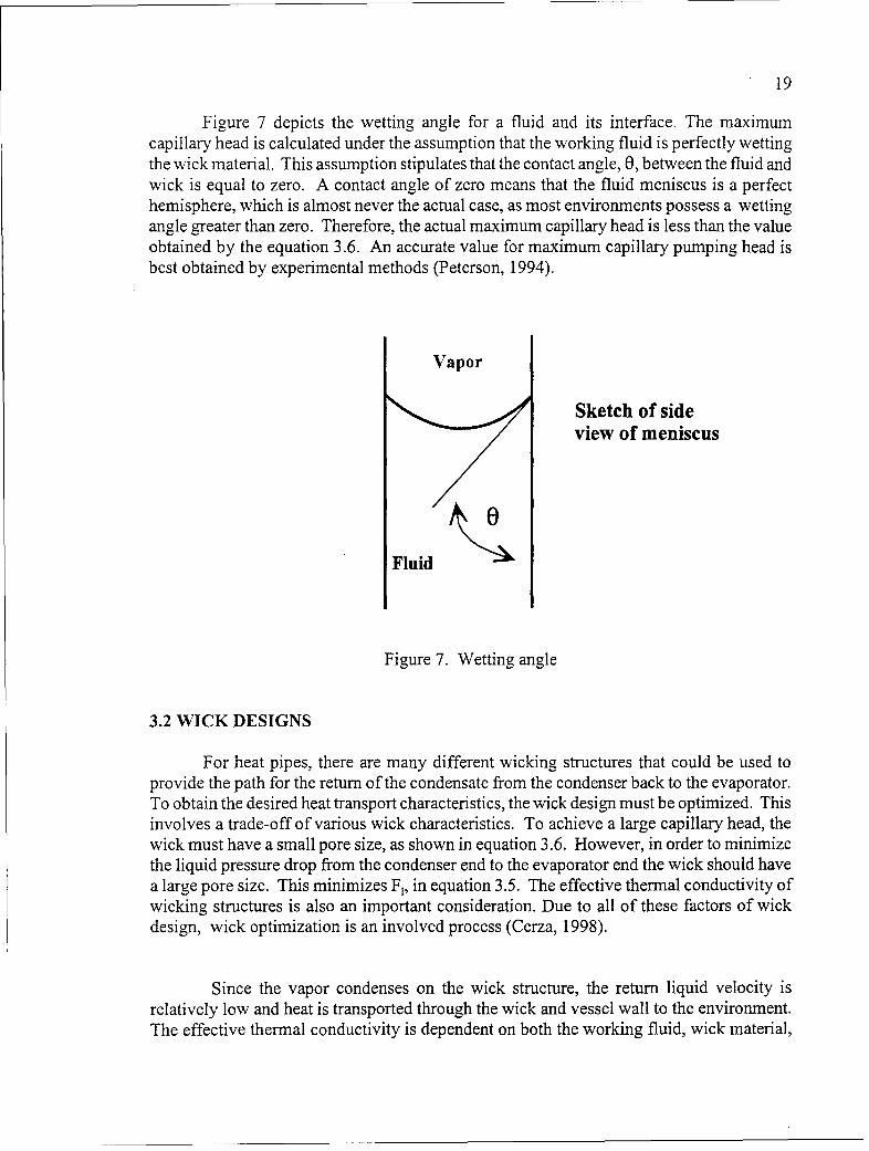
Figure 7 depicts the wetting angle for a fluid and its interface. The maximumcapillary head is calculated under the assumption that the working fluid is perfectly wettingthe wick material. This assumption stipulates that the contact angle, 0, between the fluid andwick is equal to zero. A contact angle of zero means that the fluid meniscus is a perfecthemisphere, which is almost never the actual case, as most environments possess a wettingangle greater than zero. Therefore, the actual maximum capillary head is less than the valueobtained by the equation 3.6. An accurate value for maximum capillary pumping head isbest obtained by experimental methods (Peterson, 1994).

Vapor

Sketch of sideview of meniscus

Fluid

Figure 7. Wetting angle

3.2 WICK DESIGNS

For heat pipes, there are many different wicking structures that could be used toprovide the path for the return of the condensate from the condenser back to the evaporator.To obtain the desired heat transport characteristics, the wick design must be optimized. Thisinvolves a trade-off of various wick characteristics. To achieve a large capillary head, thewick must have a small pore size, as shown in. equation 3.6. However, in order to minimizethe liquid pressure drop from the condenser end to the evaporator end the wick should havea large pore size. This minimizes F,, in equation 3.5. The effective thermal conductivity ofwicking structures is also an important consideration. Due to all of these factors of wickdesign, wick optimization is an involved process (Cerza, 1998).

Since the vapor condenses on the wick structure, the return liquid velocity isrelatively low and heat is transported through the wick and vessel wall to the environment.The effective thermal conductivity is dependent on both the working fluid, wick material,

20

and number of pores per unit area. It is the effective thermal conductivity that allows for thecalculation of the maximum wick thickness for desired operating temperatures since theeffective thermal conductivity determines the temperature drop across the wick for givenconditions. Effective thermal conductivity is found using equation 3.11 (Faghr, 1995):

(3.11)

k (k + ___+_(I_-_(o_(__ - __

where porosity, y, is wick open area divided by total wick area.

The number of wicking structures in existence vary widely. However, theycan be divided into two basic categories: homogeneous and composite wicks. Ahomogeneous wick is constructed of a single basic material. Common homogeneous wicksare the wrapped screen wick, which consists of one or more layers or screen in contact withthe vessel wall; powdered metal wicks, which are metal powders sintered to the vessel wall;and the grooved wick, which consists of grooves machined into the inner wall of the heatpipe. Homogeneous wicks also can contain arteries, or tubes to provide liquid return pathsof very low flow resistance. Composite wicks are made up of several wick materialscombined to formn a composite wick structure. Examples of composite wicks are overlappingscreens of varying porosities or a groove wick with a fine pore screen on top of it. Manydifferent composite wicks have been developed for specialized applications (Faghri, 1995).

The working fluid of the heat pipe itself must also be determined. For varyingtemperatures and heat pipe internal pressures, different working fluids will transfer unequalamounts of heat due to dissimilarities in surface tension, density, enthalpy of vaporization,and viscosity. These properties are grouped together in the figure of merit, equation 3.12(Chi, 1976):

(3.12)

M- P icy hfg_

Equation 3.12 can be used to determine which fluid will have the greatest heat transportcharacteristics for the desired operating temperature. Table 1 shows various properties andfigures of merit for various different fluids over various temperatures. Several computercodes exist that can predict some steady-state operating limits of a heat pipe if given thematerial and working fluid data for conventional, one-dimensional heat pipes.

21

Table 1. Figure of Merit Calculations

Ethanol(OF) (°C) (Pa) (kg/mA3) (J/kg) [(N*s)/mA2] (N/m) (WImA2)

T Pv rho I Hfg Mu-I surf. Tens M

68 20 5.80e+03 8.00e+02 1.03e+06 1.20e-03 2.28e-02 1.568e+10104 40 1.80e+04 7.89e+02 1.Ole+06 8.19e-04 2.1Oe-02 2.047e+10140 60 4.72e+04 7.70e+02 9.89e+05 5.88e-04 1.92e-02 2.486e+10176 80 1.09e+05 7.57e+02 9.60e+05 4.32e-04 1.73e-02 2.910e+10212 100 2.26e+05 7.30e+02 9.27e+05 3.18e-04 1.55e-02 3.298e+10248 120 4.29e+05 7.1Oe+02 8.86e+05 2.43e-04 1.34e-02 3.467e+10

Water68 20 2.34e+03 999 2.45e+06 1.00e-02 7.29e-02 1.786e+10

104 40 7.37e+03 993.05 2.41e+06 6.51e-04 6.95e-02 2.549e+11140 60 1.99e+04 983.28 2.36e+06 4.63e-04 6.61e-02 3.309e+11176 80 4.74e+04 971.82 2.31e+06 3.51e-04 6.27e-02 4.008e+11212 100 1.01e+05 958.77 2.25e+06 2.79e-04 5.89e-02 4.557e+11248 120 1.99e+05 943.39 2.20e+06 2.30e-04 5.50e-02 4.966e+11

Ammonia

68 20 1.06e+06 600.2 1.16e+06 1.41e-04 2.02e-02 9.966e+10104 40 1.42e+06 584.6 1.11e+06 1.26e-04 1.80e-02 9.295e+10140 60 2.42e+06 550.9 1.Ole+06 1.02e-04 1.37e-02 7.510e+10176 80 3.86e+06 512.3 8.95e+05 8.32e-05 9.60e-03 5.290e+10212 100 5.87e+06 465.5 7.45e+05 6.85e-05 5.74e-03 2.906e+10248 120 8.60e+06 400.2 5.29e+05 5.03e-05 2.21e-03 9.302e+09

Methanol

68 20 3.00e+04 791.5 1.19e+06 5.78e-04 2.26e-02 3.686e+10104 40 6.00e+04 774 1.16e+06 4.46e-04 2.09e-02 4.222e+10140 60 1.10e+05 755.5 1.13e+06 3.47e-04 1.93e-02 4.750e+10176 80 2.20e+05 735.5 1.08e+06 2.71e-04 1.75e-02 5.150e+10212 100 4e+05 714 1.03e+06 2.14e-04 1.57e-02 5.395e+10248 120 6.60e+05 690 9.71e+05 1.70e-04 1.36e-02 5.362e+10

22

4.0 FLAT HEAT PIPE PROPERTIES

Flat heat pipes are very similar to cylindrical heat pipes. The only real differencebetween the two is geometrical. While this may seem a minor difference, it presents manychallenges from a theoretical, engineering standpoint.

Typically, heat pipes are used to transfer large amounts of heat across a large distancewith only slight energy loss. The cylindrical design works well to serve this purpose.However, when designing an emitter for a TPV energy conversion system, it is advantageousto have a large surface area to volume ratio in order to maximize power density of thesystem. A flat heat pipe was conceived for this purpose. Flat heat pipes are a newtechnology, with few theoretical models. Flat heat pipes are also relatively untested fortransferring heat from one end to the other (as opposed to side to side transfer). Due to thedifferent surface area geometry, flat heat pipes also have different flow and structural designconsiderations than those of cylindrical heat pipes. This chapter quantifies these differencesand allows for consideration of these dissimilarities in heat pipe design.

4.1 FLAT HEAT PIPE HEATING LIMITS

Flow properties in cylinders are much different from those in rectangular geometriessuch as flat plates and/or boxes. The flow of a thin film over a flat sheet (such as in theliquid return loop of a flat heat pipe) is not the same as the flow of a cylindricalcircumferential film (which corresponds to a cylindrical heat pipe), having different frictionfactors and flow restrictions. Also, vapor flow through a cylindrical space differs greatlyfrom vapor flow through an object with a rectangular cross section, having dissimilar frictionfactors and flow restrictions. The flow property differences can present major complicationsfor flat heat pipe design, as they alter steady-state operating limits.

The limit most affected is the capillary limit. This is significant because the capillarylimit is usually the highest heating limit that a heat pipe is designed to operate at in steady-state conditions. The capillary limit involves the flow of the liquid in the wick's return pathand the pressure loss of the vapor and liquid through their respective areas of the heat pipe.Also, since the USNA flat heat pipes do not have adiabatic sections, a more accurateapproximation of the mean liquid return length in the wick was needed. The derivations ofthe various components of the capillary limit for assumed laminar flow in a flat, rectangularheat pipe are shown in Appendix 1. The capillary limit for a flat heat pipe, when only oneside of the evaporator region is heated is given in equation 4.1. In equation 4.1 q. ismaximum heat flux into evaporator section. Equation 4.2 defines K, the permeability for awire mesh wick. To achieve a large capillary limit value reff, the effective pore size of thewire mesh in the wick, must be minimized to achieve a large capillary pumping head.Decreasing reff also decreases permeability, which can lower the capillary limit value.Proper flat heat pipe design involves optimization of both of these factors to obtain a highcapillary pumping head while still maintaining an acceptable permeability value. Equations4.1 through 4.5 were derived by Associate Professor Cerza (1999).

23

(4.1)

2chfg 12pv /#Iq e L g2 + ÷I

reff L{pvAvrvPlAlK

(4.2)

K= 2pupAýp1Vp' 1f (I)

The permeability of the wire mesh wick calculated by equation 4.2 can be approximated byequation 4.3. Sample calculations were performed using both equations and it was foundthat both equations yielded nearly equal values. Therefore, equation 4.3 is preferred due toits simplicity.

(4.3)

K= 9D,

32

There are two heating configurations considered for the fullscale flat heat pipe. Thefirst involves the entire heater section mounted to one side of the evaporator region. For thisconfiguration, the capillary limit is found by equation 4.1. The other arrangement of theevaporator section consists of heaters mounted to both sides of the evaporator region. Forthis heater setup, the capillary limit is found with equation 4.4.

(4.4)

q 2- o--- 220hj lA,,2+2p ,A

eff e 2p, JThis capillary limit (two heated sides) will theoretically be higher than the limit with

only one side heated, as the two sides of the heat pipe work as parallel fluid circuits, with thetotal resistance being less when both sides are heated versus applying heat to only one sidefor the same heat flux.

The boiling limit in a flat heat pipe is similar to that of a cylindrical heat pipe. Bothinvolve pressure balances at the onset of nucleation (pressure difference from bubble tovapor space through liquid in the wick). However, since the vapor area and heat input crosssection are all rectangular, the boiling limit equation for cylindrical heat pipes (equation 3.1)changes to equation 4.5 for flat heat pipes.

24

(4.5)

Qb - sat fg t

In equation 4.5, t, is the vessel wall thickness (in), k.,, is the vessel wall thermal conductivity(W/m K), and tw is the wick thickness (in).

The boiling limit can be expected to be a very large value. Flat heat pipes areconstructed of high strength metals with polished surfaces. These metals feature very smallsurface defect sizes and therefore minute nucleation site sizes for the onset of boiling. Thisdrives the maximum heat input for the boiling limit up to a large value. This limit will bemuch higher than the capillary limit, which will be retained as the maximum heating rate forthe project in consideration. However, neither of these limits will ever actually be reached,as the internal pressure (due to the temperatures reached at these heating limits) could causestructural failure of the vessel. Appendix 2 shows the boiling limit derivation.

With water as the working fluid, the entrainment and viscous limits are not anoperational limit consideration, as the physical properties of water drive the entrainment andviscous limits to very large values within this project's operating parameters (20'C to I 000 Ccondenser temperature). Furthermnore, the entrainment limit is usually not a factor in well-wicked heat pipes, since the wick retains the liquid to prevent entrainment by the vapor.Being difficult to calculate, the entrainment limit is found by balancing the shear force onthe liquid due to the vapor flow with the surface tension of the liquid. For most applications,the entrainment limit is calculated by assuming the Weber number equal to one, where theWeber number is a ratio of vapor inertial forces to liquid surface tension forces. One mustperform this balance at the given operating point of the heat pipe to determine if entrainmentis a problem (Peterson, 1994).

In the sonic limit, the vapor cannot travel faster than the local speed of sound in aconstant area duct. The heat input that can be delivered is therefore limited by the maximummass flow rate of the vapor. To see the relatively simple derivation, see Appendix 3. Thesonic limit is found by equation 4.6, where Tiocai1 is the local temperature (K) and R is the gasconstant for the vapor [kJ/(kg K)]:

(4.6)

Q,=,D P, Ahfg kloa

25

4.2. FLAT HEAT PIPE STRUCTURAL CONSIDERATIONS

A flat heat pipe has structural problems that are not associated with cylindrical heatpipes. Cylindrical heat pipes are considered natural pressure vessels due to their shape, andcan withstand large pressure differences as well as the resulting compressive or tensile forceson their walls. Since heat pipes can exist at pressures lower than atmospheric pressure whennot in use, and can exceed atmospheric pressure at elevated, in-use temperatures, thecylindrical design has clear advantages. In this case, one of the flat heat pipe's advantages-alarge surface area to volume ratio-is detrimental to its structural integrity. The heat pipe'ssurface area is subjected to the pressure difference created between the heat pipe internalpressure and the external environmental pressure. This may result in a large force acting onthe vessel, which can cause material failure. This was clearly a design consideration thatneeded to be solved.

The design operating point for the flat heat pipes in this project was one atmosphereof differential pressure, with design case for loading taken at a near perfect vacuum. In thisscenario, the 101.325 kPa (14.67 psia) of atmospheric pressure would be acting to deformthe heat pipe with nothing more than structural supports to counteract the pressure. Sinceone of the project goals was to design structural supports that did not inhibit two-dimensionalflow, any internal beams or walls were ruled out as internal supports. This left only pinsupports as an option. Not knowing how the pins were to be fastened to the vessel wall inthe final design, the pins were modelled as both welded (rigidly attached) and not welded tothe vessel wall. The vessel wall was then modelled as a beam, with either the side vesselwall and a pin or two pins acting as supports. This gave the maximum expected deflectionfor the flat heat pipe of a given thickness, material, and spacer distance. A spreadsheet wasdeveloped to analyze deflections for many different materials, material thicknesses, and pinspacing. To view the derivations and a sample spreadsheet, see Appendix 4.

Beam deflection was not the only structural analysis conducted. To determinewhether or not deflection was the limiting factor, a column buckling analysis for pins ofvarying lengths, diameters, materials, and types of attachments also had to be conducted.However, this calculation is only necessary to reinforce the value obtained from thedeflection problem, and was performed solely on the case for which a solution was obtainedvia the beam deflection problem. The equations necessary for this calculation are readilyfound in the Strength of Materials textbook by Ferdinand Singer (1962).

26

5.0 USNA FLAT HEAT PIPE

The corporate sponsor funding this project instilled certain guidelines for the flat heatpipe being constructed. They determined the dimensions, which are 1.22 mn (48 inches) longby 30.48 cm (12 inches) wide by 1.27 cm (1/2inch) thick. They also decided that the vesselmaterial, structural supports, and wicking material be made of Monel R-400. Due to facilitylimitations, safety issues, and difficulties in working with liquid metal heat pipes, the USNAheat pipe was established as a low temperature heat pipe. Therefore, distilled water waschosen to be the working fluid, as it has the highest figure of merit of any of the candidateworking fluids at the operating temperature (1 00'C). Since effective thermal conductivityis not as important an issue to this design as maximizing capillary pumping performance, itwas decided to construct the USNA flat heat pipe with a composite wick consisting of twoMonel 400 screens of different porosity. The screen at the liquid-vapor interface will be 120x 120 square mesh (N= 120) to provide a large capillary pumping head, and the screen incontact with the vessel wall will be 40 x 40 (N=40) square mesh to provide a path of lowflow impedance. In order to counteract the crushing force of the atmosphere when the heatpipe is not at operating temperatures, Monel pins were used for internal column supports.As discussed earlier, pins offer structural support without biasing the flow towards anydirection.

Initially, the desired wall thickness and pin spacing diameter was not known. Tosolve these problems, two different spreadsheets were used. The first modelled the area inbetween the first pin from the wall. The second the spacing between the pins. Thederivations of these modelling conditions and the equations that were solved for in terms ofpin spacing and material thickness are included in Appendix 4 and are also discussed insection 5.2. Using a targeted maximum deformnation of 0. 15875 cm (1/16 of an inch), it wasfound that 0. 127cm (0.050 inch) thick Monel sheets would be sufficient with three inch pinspacing. The three inch spacing is also convenient because three is a multiple of twelve andwill allow uniform pin spacing throughout the entire pipe.

Once the pin spacing was determined, it was necessary to solve for pin diameters.Initially, the pins were only going to be welded on one side to the vessel and wick. Thusthey were modelled as colurmns rigidly attached on one end and free on the other. A columnbuckling analysis was performed for the maximum loading conditions as well as compressivefailure. A factor of safety was built into the analysis since it was assumed that the pinsexisted in a perfect vacuum (when in reality there will only exist the partial pressure of waterfor the given temperature) and support the entire crushing force of the atmosphere. It wasalso assumed that all of the pins adjacent to the pin being analyzed would fail, and that itwould bear the weight of the entire grid surrounding itself to the adjacent pins. It wasdiscovered that compressive failure would be the limiting factor for the pins, and their properdiameter was determined from this analysis. The minimum pin diameter using this methodwas found to be approximately 0.3556 cm (0.14 inch). However, it was not possible tolocate a vendor that could supply rigid Monel pins with diameters this small. The smallestdiameter readily available was 0.63 5cm (0.25 inch) and this is what was used to create theUSNA flat heat pipe. This also provides a factor of safety for failure due to buckling.

27

5.1 USNA FLAT HEAT PIPE HEATING LIMITS

Using equations 4.1, 4.3, and 4.4 explained in section 5.2 and derived in theappendices, the capillary limits are as follows:

= 42697-,w

for the case with only one side heated and

4e = 85391 w-

for the case with both sides heated.

For the case with only one side heated, with the given heater area, this results in amax heat input of 3967W, and 7933W for the case with both sides heated.

The bqiling limit, defined by equation 4.5 and the derivations in Appendix 2, iscalculated to have a maximum heat input of 9527W assuming a typical nucleation site radiusof 2.5 x 10-4 m

The sonic limit was calculated as 325,042W using HTPIPE, a one-dimensionalsteady-state heat limit prediction program for heat pipes. HTPIPE was not accurate for theother heating limits due to approximations that one must make to input parameters into theprogram which can not accurately account for the composite wick construction.

There are no standard methods of construction for flat heat pipes, as they are arelatively new and unique device. To help remedy this, a subscale model was designed andconstructed to help facilitate the fabrication process with the fullscale model. Although notnecessary, the subscale model will have internal pin supports. These exist solely to designthe final construction procedure for attaching these pins to the vessel wall in a manner wherethey will provide the intended structural support. This subscale model also has a fitting oneach end to perform charging experiments and perfect the evacuation and chargingprocedure. The subscale model will also be used to calibrate laboratory equipment whilewaiting for the construction of the final design. The subscale model is a fully functional flatheat pipe and will provide useful data to contribute to the overall mission of the project.Figures 8 - 11 depict the subscale and fullscale heat pipe designs.

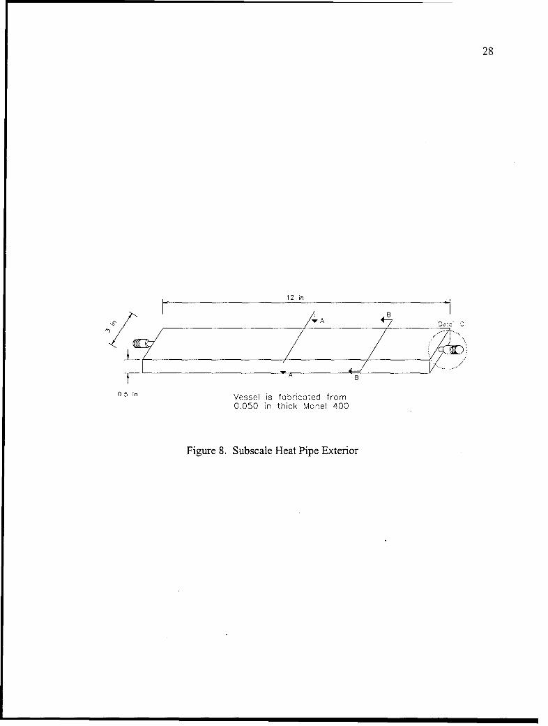
28

12 in

F- A A

0.5 in Vessel is fabricated from0.050 in thick Monel 400

Figure 8. Subscale Heat Pipe Exterior

29

Note: Figures are not drcwn to scale

-i in View A-A

________Pins are s.-ct-ne~cec:__! , ',: , on top of screen to nesse!'_...________,II ; ' ': ... . . . ... _______ _:__attaching both pin cnt

Sscreen to vesse! cul

Upper ScreenLines c!I wcils 3 in

120 x 120 sauare meshMore, 400

Monet 400 pin s•coo."s

View 8Eo-B.257 in l dcr, Detail CBottom Screen 0

lin e s e il w o rl s 3 t o t

40 x 40 sc~cre mesh wMore• 4CCl

ooenCO5a lorge as snoo 0.75 in (19 mm)con fit into c and mole threoCec erlcmointoin seci o fit hi-vec eeoi volve

1.5 9. a HE

Figure 9. Subscale Heat Pipe Interior

30

48 in

0.5 in 8

Figure 10. Fullscale Heat Pipe Exterior

31

Note: Figures are not drawn to scale

3 ri, View A-A 3 in

.Pins are sot-weioec

S.: :s creen to vessei woll

Upoer ScreenLin es c !I w allst20 x 120 square mesnMonei 4CO

Monel 400 pin sunoortsView B-8 0.25 in diameter

BoVtom Screen 0.3572 in tal Detail Clinesoial weels 45 toto (3 wide x 15 long)

4C0 x 40 square mesn -Monlel 400 os lorce as snas I 0.75 in (1 9 mrr)

can fit into end and |mole threadea e..-F.Maintain seal Pto fit ni-vac bal valve

3in 3in (fits internally) 1i]

Figure 11. Fuliscale Heat Pipe Interior

32

6.0 SUBSCALE FLAT HEAT PIPE

After the necessary supplies were obtained, the fabrication and assembly phase couldbe carried out. The subscale heat pipe was constructed first. Its purpose was to providepractical experience of fiat heat pipe construction as well as be used to help calibrateinstruments and set up the laboratory spaces. In addition, it aided in proving the practicalityof the design and revealing and structural faults.

6.1 SUBSCALE FLAT HEAT PIPE CONSTRUCTION

The basic approach to construction was to assemble the heat pipe in two separatecomponents. This involved drilling all the holes necessary for the pin supports, bending thesides of the two halves to the proper dimensions, and attaching the two layers of screen. Theend pieces and fittings were also fabricated at this time and the pins were cut to the properlengths and deburred. Then, the two sides were welded together, the ends welded on, andthe fitting welded in. After this, the pins were inserted and welded to both sides of the heatpipe from the outside.

The subscale heat pipe was constructed mostly to the above parameters. The monelsheets were bent using twelve inch long copper bars with edges of fine radii. The screen wasthen cut to the same size using metal shears and taped to the vessel material. They were thentack-welded into place, centered halfway in between pin locations. Next, the 0.635 cm (1/4inch) holes for the three spacers were carefully dimensioned and drilled in both halves throughthe vessel material and the screen. This created some problems with the screen integrityaround the hole as well inducing stress around the tack weld spots. However, these werevery minor and not enough to substantiate reattaching different screen material as the screenstill maintained good pore integrity and contact with the vessel wall. This meant that the wickwould still produce sufficient capillary pumping action and the effective thermal conductivityof the screen would remain as high as possible. The end fittings for the high vacuum ballvalves were then machined and the endpieces and the pin spacers were then cut. However,they required extensive deburring and grinding so that they could fit into the 0.635 cm (1/4inch) diameter spacer hole.

After the subscale fiat heat pipe's constituent elements were readied, the two halveswere welded together. The welds were staged from side to side so that the warping due tothermal stress would be minimized. The ends were then welded on, and the fittings wereattached in the proper place. Following this, the pins were Tungsten Inert Gas (TIG) weldedto both sides of the vessel wall from the outside.

6.2 SUBSCALE HEAT PIPE TESTING

Once 6ompleted, the subscale was pressure tested for leaks. The pins presented aproblem, as did the end fittings. To make an airtight seal, the end fitting design had to be

33

alterred. The tubes that extended from the heat pipe were cut, and the fittings were weldeddirectly to the ends of the heat pipe. The pins were welded to both sides of the vessel, as itwould have been very difficult to attach the pins to only one side of the heat pipe. Thisreduced the calculated deflection substantially, and would later do the same for the finalmodel.

The pins required re-welding several times in order to create an airtight seal at thedesired 1 atmosphere of gage pressure. This problem of rewelding was found to be inherentto the design by both welder and design team. The pins were necessary for structural integrityand had to be welded from both sides to ensure structural support. Reheating of a completedweld by welding on the opposing side was determined not to be a pertinent issue since thetype of welding utilized featured the use of localized heating for a short period of time. Thiswould not be sufficient to heat the opposing weld spot to a temperature at which it could startto loosen (Monel welding wire or sheets would liquefy).

The subscale heat pipe was not intended to be used for extensive experimental data-taking, but to be used to verify, that the basic heat pipe design worked, to find design flaws,and to setup laboratory equipment. Therefore, its testing regime was not very expansive. Itstesting regime and objectives were as follows:

1. Design a reliable, easily repeatable method of leak-testing and make the subscale heat pipeleak-free.2. Evacuate the heat pipe. Attach a pressure gauge to the evacuation apparatus and measurethe level of evacuation achieved.3. After successful evacuation, design and construct a charging apparatus for accuratelycharging the heat pipe with the correct amount of working fluid and sealing it off aftercharging. This method must be easily repeatable.4. Apply a heat source to one end of the heat pipe and check for response. The condenserend will achieve a temperature nearly the same temperature as the end with the applied heatsource. It is advisable not to use anything more than hot water for this test as it is conductedby hand.5. Submerge one end of the heat pipe in a hot water bath. Monitor the water bathtemperature and the heat pipe by quantifiable means. Also monitor the heat pipe performancewith the infrared camera to determine if it is working properly, checking for end effects thatmight indicate a leak or improper charging and temperature variations that signal interiordefects or improper charging.

6.3 SIJBSCALE HEAT PIPE TESTING RESULTS

The leak-testing and charging consisted of the fabrication of a charging apparatus.A 0.635 cm (1/4 inch) nipple was fitted to the end of it (with necessary reducer) and matedto the compressor. The heat pipe was then pressurized for leak testing. Valve 2 in the

34

charging apparatus (see Figure 12) could be throttled so that excessive pressure did not buildup in the heat pipe. A pressure gauge was fitted temporarily to the charging apparatus nearthe heat pipe to calibrate the throttling and was removed at the time of this picture. To leaktest, soapy water was applied to the pressurized heat pipe in order to detect the leaks. Leakswould form bubbles in the soapy water. This assembly could be mounted and removed fromthe heat pipe with a few hand tools.

Figure 12. Charging Apparatus

Charging the heat pipe with working fluid was performed fairly simply as well. Tocharge a heat pipe the wick must be completely saturated. First, the heat pipe and chargingassembly were mated to the vacuum pump and evacuated with valve 2 closed. In the fluidcharging column was placed the correct amount of water to charge the heat pipe. Theseamounts were measured and marked (observe gradations on fluid charging column), takinginto account the volume that would occupy the fittings as well as the heat pipe. Onceevacuation was complete, valve I and the valve attached to the heat pipe (not pictured) were

35

closed, and then the vacuum pump was shut off. Valve 2 was then opened, and the vacuuminside the fittings drew the water in to fully fill the fittings. The heat pipe valve was thenopened slightly to bleed in the necessary charge (as marked on the column). All valves werethen closed, and the charging apparatus removed if necessary, taking care not to disturb thevalve connected to the heat pipe (as it holds the heat pipe to the proper internal conditions).It is important to note that all valves used were rated for special high-vacuum service. Toverify the time required for charging the heat pipe, the mass flow rate at 6.9 kPa (Ipsia) wascalculated for water vapor through the 0.63 5 cm (1/4 inch) hole in the end fitting throughwhich the pipe was evacuated. The vacuum pump's flow rate was found to be the limitingfactor in evacuation, not choked flow conditions. This condition would remain true for thefuliscale heat pipe as it was to have the same size end fitting.

The finished, testable model of the subscale flat heat pipe appears in Figure 13. It isshown with a valve still attached to it to show how they are mounted. Note the absence ofthe tube in the end fitting. The heat pipe is painted flat black to raise its surface emissivityso it can be viewed best by an infrared camera.

Figure 13. Subscale Heat Pipe

After all leaks were eliminated, and the heat pipe was successfully charged, it wassubjected to a hot water bath. Within seconds, the other side of the heat pipe began to warmup. It worked at least as a crude heat pipe. After this, it was submerged in a pot of boilingwater and monitored with the infrared camera. This facilitated a qualitative check of the heatpipe performance as well as calibrating and learning how to use the infrared camera. Thesubscale passed this test flawlessly, showing an almost isothermal condenser section with

36

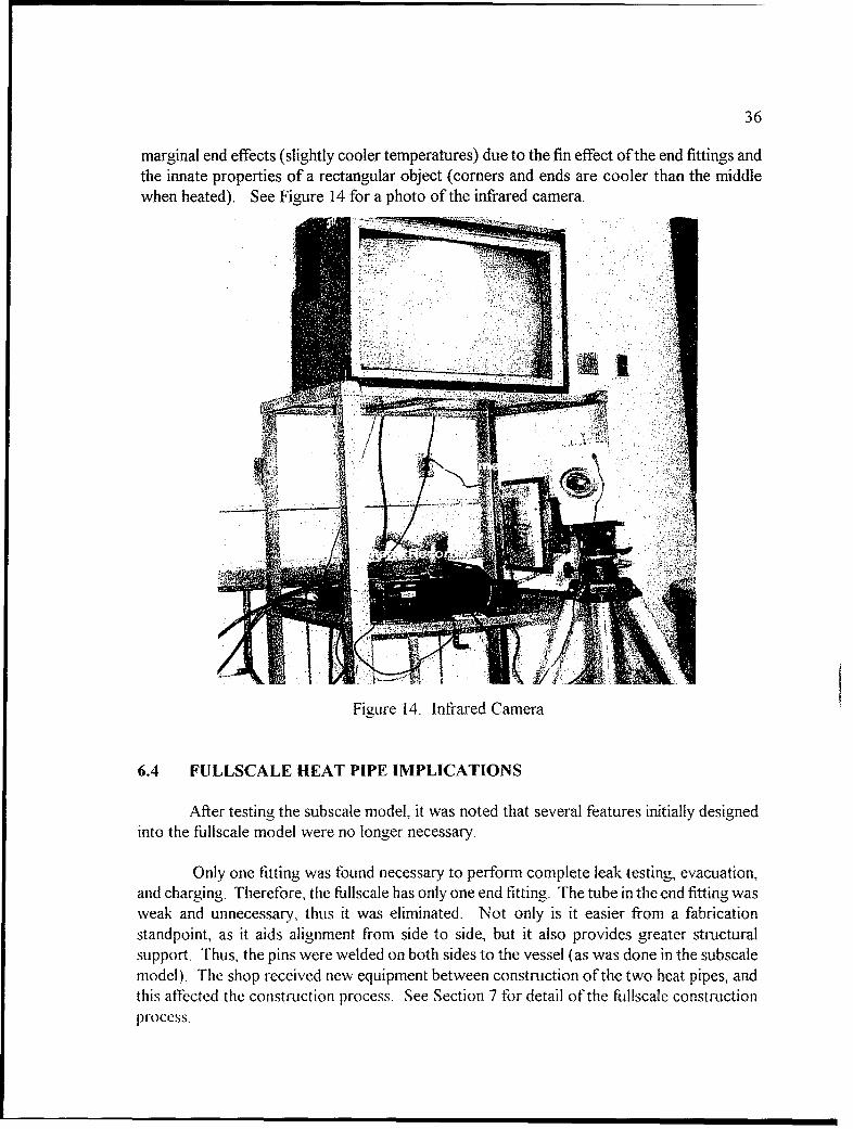
marginal end effects (slightly cooler temperatures) due to the fin effect of the end fittings andthe innate properties of a rectangular object (corners and ends are cooler than the middlewhen heated). See Figure 14 for a photo of the infrared camera.

Figure 14 Infrared Camera

6.4 FULLSCALE HEAT PIPE IMPLICATIONS

After testing the subscale model, it was noted that several features initially designedinto the fuliscale model were no longer necessary.

Only one fitting was found necessary to perform complete leak testing, evacuation,and charging. Therefore, the fullscale has only one end fitting. The tube in the end fitting wasweak and unnecessary, thus it was eliminated. Not only is it easier from a fabricationstandpoint, as it aids alignment from side to side, but it also provides greater structuralsupport. Thus, the pins were welded on both sides to the vessel (as was done in the subscalemodel). The shop received new equipment between construction of the two heat pipes, andthis affected the construction process. See Section 7 for detail of the futlscale constructionprocess.

37

7.0 FULLSCALE HEAT PIPE CONSTRUCTION

The fullscale model was to be constructed differently than the subscale model. Thiswas due to Technical Support Department's acquisition of a new CNC Punch-Press machineas well as experimentation with the subscale and a visit from the corporate sponsor.

7.1 FULLSCALE HEAT PIPE CONSTRUCTION DETAILS

After the screens and Monel sheets were cut to the proper dimensions, their size andassigned hole placement were loaded into the CNC Punch-Press machine's user interface. TheMonel sheets for the vessel wall were punched first, making holes in the locations where pinswere to be welded. Next, to avoid any tearing, stretching, or any other kind of deformationin the screen, the screens were laid on top of each to other, taped to the side of thin steelsheets (3rOmil), and sandwiched in between the sheets. They were then loaded onto the CNCPunch-Press machine and were punched in the appropriate places, so that the steel sheetsabsorb the initial impact and prevent the movement and subsequent deformation of the screen.By using the computerized machine, it was possible to place all of the necessary holes inexactly the correct spots on both the sheets and the screen to ensure that the sides would lineup perfectly.

Long copper bars with fine radius edges (same radius as used in construction ofsubscale) were obtained to facilitate bending the ftillscale heat pipe to the requireddimensions. The two layers of screen were then layed on top of the vessel, fastened with tapeon the ends, and fastened down to the vessel by threading small screws through the pin spacerholes and attaching nuts on either sides. The screen was then tack-welded to the vessel wallin regular intervals between the pin spacer locations. Keeping the screen flush and in contactwith the vessel presented a challenge, and a small portion of the screen on one side of the heatpipe ended up being not in contact with the vessel, but detached from the vessel in a smallsection of the heat pipe. This spot was noted in case it caused any performance problems.Figure 15 shows a close-up photo of the tack welds and the holes drilled for pins in a Monelsheet, and Figure 16 shows the two completed halves lying on top of each other. The endpieces and fitting were machined. Figure 17 shows a completed half with visible screen andbent side. The pins were then cut to the proper length, milled, and deburred to fit into thenecessary space. Figure 18 shows the pins standing on the vessel wall before this process.

With all of the necessary components ready, the assembly began. First, the sides ofthe two separate halves were welded together, carefully sequencing the welds and using aheat trap to minimize deformation. After this, the ends were welded on, and the singular endfitting was welded snug to the end to resemble the final appearance of the subscale heat pipe.Following this, the pins were placed in their proper spots and TIG welded from either sideof the heat pipe. The experimental setup then began.

3 8

Fig-ure 15. Monet sheet close-up

FiguLre 1 6. Completed H-alves

39

Fig~ure 17. Screen-Side view with Bent Side

Fig~ure 18. Sheet with Pins

40

8.0 EXPERIMENTAL SETUP AND PROCEDURE

The setup for experimentation as well as the procedure for experimentation werecomplex parts of the project and had great importance to the success of the project. It wasvery important to verify that the flat heat pipe does indeed perform as a heat pipe and to takedata on its one-dimensional performance before proceeding on to any other tests. These one-dimensional tests were also the easiest way to understand and interpret the internal dynamicsof the heat pipe as they influenced the temperature profile. Next, as the impetus behind theIproject was to examine two-dimensional flat heat pipe behavior, asymmetric heatingconditions were imposed and the experiments run. A heat pipe is, by definition, a hermeticallysealed vessel that transfers heat via phase change processes and has capillary pumping actionIto circulate the working fluid. It was necessary to test this capillary action. As mentionedearlier, the capillary limit is also the desired operating limit for most heat pipes. Finding the

capillary limit of the heat pipe is therefore very important to not only understanding heat pipeperformance but also to maximizing heat pipe performance. Experiments were conductedat differing angles of gravity assist for the liquid return path to test the capillary pumpingaction of the screen and gravity's effect on the heat pipe's performance.

8.1 EXPERIMENTAL SETUP

The asymmetric heating case was a unique case. The heaters had to possess theflexibility to be reconfigured and turned on and off independently to be able to satisfy boththe symmetric and asymmetric heating cases. To meet this need, 16 high temperature 500Watt strip heaters 1.905 cm (3/4 inch) inch wide with a heated section of 30 cm (11 13/16inches) were purchased. They were wired in blocks of four to variable transformers, andcould therefore be moved in blocks of four and have their heating rate adjusted independentlyin four blocks of four heaters each. The variable transformers were also wired to Wattmeters,which were wired into junction boxes (to be detailed later). The electric signals from theWattmeters were recorded by the computer to which these junction boxes fed.

Thermal joint compound was spread between the heaters and the heat pipe to lowercontact resistance and ensure that most of the generated heat went into the heat pipe. Theheat pipe was then insulated with a ceramic tile over the heater sections with aluminum foilinsulation wrapped around the entire assembly. To view the heaters being mounted withthermal joint compound in the symmetric case (all heaters on one side, covering the entirewidth) see Figure 19. Figure 19 does not show all of the heaters mounted to the heat pipefor the symmetric cases. Instead, Figure 19 shows ten of the heaters mounted and the thermaljoint compound that was part of the heater section fabrication. Figure 20 shows thecompleted asymmetric mounting (half of the heaters on each side, covering only half of oneend with the heaters covered with a ceramic tile and aluminum foil insulation).

41

Figure 19. Symmetric Heater Mountingy

FILiLure 20. Asymmetric Heater C0onhgUration

42

The same evacuation and charging assembly that was developed for the subscale heatpipe was used for the fullscale heat pipe. A photo of this assembly is shown in section 6. Torecord saturation pressures inside of the heat pipe, a pressure transducer was mounted to theend of the heat pipe in between the heat pipe valve and the heat pipe itself Figure 21 showsthis end fitting with the transducer mounted. This transducer was used to record most of thedata. However, this transducer malfunctioned, and was replaced by an analog pressure gaugeas seen in Figure 22.

S.'

Figure 21. Heat Pipe End Fittings

43

Figure 22. Analog Pressure Gauge

Again, it is important to note that the valve used was specially rated for high vacuumservice. A regular valve would not be capable of holding the high vacuum states that occurin evacuation and when the heat pipe is properly charged but not operating.

Since testing at various angles to the horizontal is an important part of the test criteria,it was necessary to design a test stand such that the heat pipe was capable of rotating throughthe required angles while remaining free to natural convection. For this, a wooden stand wasdesigned that consisted of two legs fixed to a flat base. See Figure 23 to view the stand withheat pipe mounted. Attached to the stand were two clamps to hold the heat pipe in placewhile being able to rotate it. These were made from two C-Clamps welded together by a steelbar. From this bar protruded a threaded screw, which was fixed to the bar. This screw wentthrough a wooden bearing block and the test stand legs, and was attached on the other sideof the leg by a wing nut and a washer. The wing nut could be loosened and tightened tomove the clamps through the various angles about the screw. This assembly rotated the heatpipe through the required test angles, Figure 24 shows the clamps mounted to the heat pipewith PVC feet attached. These PVC feet served not only to spread the load, but also toinsulate the clamps from the heat pipe so that the clamps could not become a heat sink.

Temperature data were recorded in two ways. The first was via the infiared cameravideography, pictured in section 6. The other means was by an array ofthermocouples. The

44

placement of the thermocouples on the heat pipe are shown in Figure 25. Figure 26 showshow the thermocouples actually looked when mounted on the heat pipe. The numbers of thethermocouple locations correspond to their assigned numbers in the data collection software.The thermocouples were wired into the same data acquisition junction boxes used by theWattmeters. There were 8 junction boxes with 8 channels each for a total of 64 channels ofdata sampling. However, only 43 were used (39 thermocouples plus four Wattmeters). Tosee how the system is configured, see Figure 27.

Figure 23. Heat Pipe Test Stand

45

Figure 24. Heat Pipe Mounted to Clamp

46

CM offset from centerline11.4 3.8 3.8 11.4 11.4 3.8 3.8 11.4

Initial: IRHeate' Camer

S1Side.

Heatersection

34.3I• I• 'A 4 S i - 41.9

-,*7 1 . :14 26

, * |offset

S 2 , ,' from1 22* -- 64.8 heater

end

23 2A2s12 25 26 80

29 30 3a 32 ' 95 3

,0_ ,_,___•-110.5

'7LY i'End Fitting LI •7 Room Air

Figure 25. Thermocouple Placement by Number

__ 47

Figure 26. View of Attached Thermocouples

Vyatmeters

- "'A

u~n Ion Boxe

Data recording

FigLIIC 27. Testing Setup

48

8.2 EXPERIMENTAL PROCEDURE

The heat pipe went through tests at different orientations. Figure 28 shows thenomenclature for the different orientations.

Heater End

I z 4900, against

gavity 2 450 aaingravity

3 7

4505

900

Heater End

Figure 28. Testing Orientations

The testing criteria for the symmetric heating case (all heaters mounted on one side,covering entire width of heat pipe) was as follows:

1. With 100% fluid charge, test orientations 2,3,4,5,6, and 7 heating slowly to at least 400Watts (more if conditions allow), allowing heat pipe to reach equilibrium temperature for eachheat input.2. With 125% fluid charge, test orientations 3,4,5, and 7 heating with at least 400W allowingequilibrium conditions.

49

3. With 75% charge, test orientations 3,4, and 5 heating with at least 400W allowingequilibrium conditions.4. Mounting the heaters in the asymmetric configuration (see Figure 20), test heat pipe with100% fluid charge in orientations 3,4, and 5 heating slowly to as high a heat input as possible,allowing for equilibrium between heating increases.5. For all runs, data is to be collected over time by data acquisition software, which recordscontinuously, and the infrared camera, which records at the user's discretion.6. Take video and still photographs of interesting phenomena via the inifrared camera.

50

9.0 DATA ANALYSIS

The experiments detailed in chapter 8. 0 were completed. However, some calculationshad to be performed before the data could be properly analyzed.

A fin, whether it is an isothermal heat pipe fin or a conventional fin, rejects heat to theambient by means of convection and thermal radiation. These heat rejection modes arerepresented by equations 9.1 and 9.2, respectively (Kreith and Brohn, 1997). In equation 9. 1,h is the convection coefficient [W/(m K)], A is the surface area of the body, and AT is thetemperature difference between the hot body and its surroundings. In equation 9.2, Cy is theStefan-Boltzmann constant, e is surface emissivity (percent radiated as compared to an idealemitter), Th is the temperature of the radiating body, and T~,b is the ambient environmenttemperature.

(9.1)

Qcorw " AA T(9.2)

Qrad =CTA(Th T 4c6)

For radiation heat transfer, the emissivity is set to .95, a value experimentallydetermined for the heat pipe using the infrared camera and thermocouple measurements. Thiswas done by comparison of thermocouple measurement to infrared measurement. Emissivityis adjusted in the infrared camera data menu until the temperatures seen by the infraredcamera match the temperatures recorded by the thermocouples.

Tables and equations used in solving the combined convection-radiation heat rejectionproblem are shown in Appendix 5. Figure 29 shows the heat transfer rejection modes for agiven heat input (Watts) assuming all heat is transferred into the heat pipe (Cerza, 1999).

From Figure 29 it is seen that both radiation and convection are important modes ofheat transfer for the heat pipe. To determine if the heat pipe was properly functioning as aheat pipe, it can be compared to a conventional fin. A fin is an extended surface that enhancesheat transfer by increasing the heat transfer surface area, such as the aluminum fins on anautomobile radiator. Thermal energy is input to the fin at one end. The energy then conductsthrough the fin to the colder end. As the energy conducts through the fin it is rejected to theambient surroundings by convection and radiation (in this case). Since convection andradiation are of the same order of magnitude for the heat input range of these experiments,the simpler convection model is used with a convection heat transfer coefficient, h, equal totwice that of the value for convection only, thus taking the radiation heat rejection mode intoaccount. Steady-state fin temperature along the fin length can then be calculated for arectangular fin by equation 9.3.

51

Heat Transfer Rejection Modes600 - _, _ ___ _ _ _

450)

J 375

150 .

75

"100 200 300 400 500 600 700 800 900 1000Qwatt.

Power In. W

convectionradiation

Figure 29. Heat Transfer Rejection Modes for Heat Input

(9.3)

7 r.: T ,,b + kAILY

where m is found with equation 9.3 as follows:(9.4)

and P is the perimeter of the fin, A, is the cross-sectional area in the x-direction.

The previous fin analysis is for a conventional fin. The heat pipe fin temperature isapproximately isothermal along the fin length. Equation 9.5 represents the steady-state,isothermal heat pipe fin relation:

(9.5)

( hA( T'- 7,'1,M ) + oa A-( 7'4 -7•',, )

Equation 9.5 is a fourth order polynomial equation for the temperature T. Thesolution to equation 9.5 is the positive real root of equation 9.5 assuming that T is unique andgreater than T,,,,,.

52

9.1 HEAT.PIPE VERIFICATION

Figure 30 shows a plot of a conventional fin vs the experimental data for the USNAflat heat pipe at a 400W steady-state condition with 100% fluid charge.

200

150

0z-1 00 Experimental Data

50 IdWa1 Heat Pipe

0-

0 20 40 60 80 100 120x distance (cm)

Figure 30. Standard Fin vs Ideal Heat Pipe Fin and Actual Heat Pipe (400 WSteady-State, Horizontal)

As one can see from the experimental data plot, the heat pipe was not isothermal, buthad about a 60'C temperature drop from the beginning of the heat pipe to the end. However,a portion of the heat pipe was nearly isothermal. It can be assumed that the heat pipe isperforming as a heat pipe for the first 80 cm away from the heater section and not as aconventional fin since the temperatures of the experimental data are close compared to thetheoretical heat pipe case. Figure 3 1 shows an infrared camera photograph of the heat pipein the horizontal (13) position (not yet reached steady-state with 125% charge). This clearlyshows that although there are some serious end effects involved, a large region of the heatpipe is fairly isothermal. It is believed that some air leaked into the heat pipe and caused theend effects (cooler temperatulre pockets) by blocking a portion of the condenser region. Athigher heat inputs (such as Pictured inFigure 3 1), the air would be compressed into the end

fitting by the water vapor, causing the cold region to recede, making the heat pipe surfacecloser to isothermal The cold spot in the middle of the photo corresponds to a section ofepoxy used to seal a leak. It is an insulator, and is therefore colder than the metal of the heat

53

pipe. The clamps that hold the heat pipe to the test stand also insulate and therefore areshown to be cooler than the heat pipe. Figure 32 is a graph corresponding to the photo inFigure 31, the best isothermal profile achieved by the USNA flat heat pipe.

Figure 31. JR Photo of Horizontal Heat Pipe, 800W, 125% Charge

200

180 K\\.........

O1 20

60.4

40

0 1 2 3 4 5time (min)

Figure 32. Near Isothermal Case Temperature Vs Time, [Horizontal, 600W, 100% Charge

54

9.2 EFFECTS OF ORIENTATION ON HEAT PIEPES

The convection coefficient, h, utilized in equation 9.5 change for flat plates with theirheated side facing downwards in accordance with their orientation. Equations 9.6 and 9.7can be used to solve for the convection coefficient at a given angle of orientation, 0, from thevertical. In equation 9.6, A'i is the Nusselt number, a dimensionless heat transfer coefficientthat is the ratio of convection heat transfer to conduction in a fluid layer of thickness L. Gr1and Pr are the Grashof and Prandtl numbers, respectively. The Grashof number is the ratioof buoyancy to viscous forces, and the Prandtl number is the ratio of molecular momentumdiffusivity to thermal diffusivity (Kreith and Brohn, 1997).

(9.6)

kNilL

(9.7)

N'il =.56(Giý Pr cos 0)

Note: equation 9.7 is only valid for 0<900

For the 90' case, equation 9.8 is to be used, where Ra, is the Rayleigh number,which is the product of the Grashof and Prandtl numbers (Kreith and Brohn, 1997).

(9.8)

Ni= .15(Ra,)1

Although the convection coefficient would be slightly higher for the heated side facingupwards due to the interaction of buoyancy and momentum effects in natural convection, thiscase will be treated as if the convection coefficient is uniform for both sides of the heat pipe.By looking at equation 9.7, one can see that convection coefficients decline as the angleincreases. Therefore, at orientations approaching the horizontal, to reject the same amountof heat, the surface temperature of the heat pipe must rise (equation 9.1). Using equation 9.7,a theoretical plot of isothermal flat heat pipe temperature versus angle orientation was madeand compared against experimental data collected for the 400W steady-state condition with100% charge (Figure 33). The experimental data is relatively close to the theoretical values.

When an orientation angle other than horizontal was introduced, the heat pipe did notdemonstrate isothermal behavior until the heat input was increased to near 600W. Figure 34shows the best isothermal profile reached for the vertical orientation (position 5). Figure 34depicts the sides of the heat pipe as much hotter than the middle portion. This condition

55

existed for all inclined cases. Figure 34 shows a temperature difference of about 27°C fromthe hottest part to the coolest part of the condenser section. The data corresponding toFigure 34 was the closest to a theoretical heat pipe of any of the inclined test cases. Figure35 shows a start-up condition (transient effect) for this orientation (position 5) at a lowerpower setting of 400W. Note the large temperature gradient across the heat pipe.

90

85

80

Uc75

v 70

c 65

60 theoretical

55* * e:.:primen tah I

50 .

6 10 20 30 40 50 60 70 80 90Angle, degrees

Figure 33. Heat Pipe Temperature vs Angle, 400W

56

99.2110.4e. 9.50img12

104.98 .6 1 ..........9Z. 485.4"177. Z".67.354.435.3

Figure 34. IR Photograph, Vertical (5), 60OW

A33.19 ingsTOR54.3

110.4950

Img 5

74.4i69.51,

I 63.9t,

50.0140.628. 0

Fiý-'Lire.3 Vertical Gradient, 40OW, 125% Charge

57

Only one case was tested with the condenser end lower than the evaporator end. Thiswas orientation 2. The heat pipe did not function properly, acting as a fin. This is becausethe maximum vertical capillary pumping height achievable by the wick is around five cm.Therefore, no water could be delivered to the evaporator region via the wick (its height wasgreater than five cm above the end of the heat pipe) and the evaporator section remained dry.Without the circulation of the working fluid, the heat pipe does not fu-nction as a phasechange device, but acts as a conventional fin. Only the horizontal tests performed well, andthis will be explained in section 9.6.

9.3 EFFECTS OF VARYING CHARGE

To compare the effects of varying charges, each charge experiment was conductedat a 400W heat input. The experiments were allowed to reach a steady-state condition fororientations 3, 4, and 5. The horizontal cases produced the best data and are presented forcomparison. Figures 36, 37, and 38 show the data plots of the each case, 125% charge, 100%charge, and 75% charge in sequence. Figure 39 depicts the three charges plotted against eachother on the same graph for a uniform heat input over time.

80.•4 1 t

70 j 9.5 9. n

60

A, . , L,.

F-5020 .. ,

30

2 4O

1010 20 30 40 50 60

time (min)

Figure 36. Temperature vs Time, 400W 125% Charge

58

180

160

140

600

80

60)40

24 0

0 20 40 60 8010121416time (min)

Figure 387. Temperature vs Time, 400W 700% Charge

59

100

80

60

Green - 75%40 Blue 125%

Red= 100%20

00 20 40 60 80 100

time (min)

Figure 39. Varying Charges Temperature Vs. Time, 400W, Horizontal

Although the differences in effects are not very pronounced, it is apparent that the75% charge case displays the quickest response time. This is because there is less water inthe heat pipe and therefore less energy to be absorbed, allowing the heat pipe to attain steadystate. However, notice that not all of the heat pipe in the 75% charging case achieves thesame operating temperatures. This could be due to a lack of fluid in the wick required tocirculate the necessary heat to activate the full heat pipe or the presence of air in the heat pipe(gas loading).

The 100% charging case has the best traditional heat pipe response. When a locationencounters the condensing vapor front, it changes temperature rapidly to the saturationtemperature corresponding to the internal saturation pressure. However, it takes longer forthe 100% charging case to reach isothermal conditions along the length of the heat pipe thanthe 125% case. This is due to the presence of air, as once it is compressed further towardsthe end of the heat pipe the temperature at the location it previously occupied increasingrapidly. Also, the 100% charging case achieves the best near-isothermal condition, as alllocations except the end are within a few degrees of each other at the steady-state condition.The divergent line on the top of the plot, corresponding to I 1.4cm, does not necessarily makethe heat pipe non-isothermal. This curve corresponds to thermocouples on the back of theheater side, and are therefore more representative of the heater temperatures. Thethermocouples were reading an averaged temperature of the hot heaters and the insideevaporator section of the heat pipe. Hence, they would indicate higher temperatures than thethermocouples on the condenser end of the heat pipe. This curve can therefore be ignored.

60

The 125% charging case theoretically should take more time for all locations to reachan isothermal condition. This is because there may be some liquid flooding in the evaporatorsection, and until it is vaporized, there can be no menisci in the wick and therefore nocapillary pumping action. The 125% charging case does reach a near isothermal case whenit reaches steady-state, though it heats up faster than the 100% charge. This is not fullyunderstood, though it is likely that the 100% charging case was conducted with more airpresent in the heat pipe than the 125% charging case, which required more time to compressthe air towards the end of the heat pipe.

9.4 START-UP CONDITIONS

Before a heat pipe can reach a steady-state condition, the energy it is receives as heatinput must heat all of the mass that comprises the heat pipe (fluid, screen, vessel wall, etc.)to the steady-state temperatures. The USNA heat pipe with a heat input of 400 W wouldrespond as shown in Figure 40. Figure 40 compares closely to Figure 37, the 400W start-upcase for a 100% charge. The experimental case reaches a slightly higher temperature in theactivated regions. This is because in order to compensate for inactive regions which are ata lower temperature the active regions must get hotter to reject the input heat. However, bothgraphs reach an approximate steady-state condition at around one hour. Therefore, Figure40 represents a good model.

Transient Start Up - 400W, Horizontal80 1 1

70

60 -6

SThpC(Thpl

40

30

200) 0.2 0.4 0.6 0.8 1

t2 (Th p IIhimc. hr

Figuire 40. Theoretical Heat Pipe Start-Up

61

Another aspect of startup is shown in Figure 41. Figure 41 includes a plot of theheaters, which is the top trace in this graph. It is interesting to note that when heat is applied,the heaters' response time is rapid. The heat pipe slowly activates more regions, and whenmany are activated, the temperature of the heater drops because heat is being more effectivelytransferred over a large area.

300

250

--rrepond router,to .W.11a

200 di[ 4.al~pip, e /"

U/ /I .4,'

0 150

100

50 11- ...

0

0 50 100 150 200 250 300time (min)

Figure 41. Temperature vs Time for 100% Charge, 400-800W, Horizontal

9.5 ASYMMETRIC CASES

Two cases of asymmetric heating will be discussed: the response of the heat pipewhen inclined, and the response when horizontal. When horizontal and at a low heat input,only the condenser area opposite the heater section activated, as seen in Figure 42. However,as the heat input rises, the heat pipe condenser region begins to become more active as seenby the increasing size of the higher temperature section of the condenser surface. Figures 43and 44 shows the heat pipe's thermal profile when the heat input is raised. This performanceis indicative of having a non-condensable gas, such as air, in the heat pipe. If the USNAheat pipe performed as a theoretically perfect heat pipe without non-condensable gasesinside, then all the condenser surface in the asymmetric (or any) case would reach anisothermal state.

62

:74.4110.4

75..70.766.-60.754.70,47.6

Z7.1 .99/03/31,12-22

Figure 42. Asymmetric, Horizontal, 20OW

38.0110.4

84.179.574.368..6,

54. 044.230.9 9/03/31 13:13ýý

Figure 43. Asymmetric, Florizontal, 40OW

63

Figure 44. Asymmetric, Horizontal, 600W

The inclined cases did not perform as well as was hoped. The condenser sideadjacent to the heaters never frully activated, and the more developed profile remained the"~side-climbing" phenomenon that was observed in early inclined cases. Figure 45 shows theside near the heater section, and Figure 46 shows the larger area's thermal profile.

Fig.ure 45. Asymmetric, Inclined, 400W

64

Figure 46. Asymmetric, Inclined, 400W

9.6 VARIABLE CONDUCTANCE HEAT PIPES

A variable conductance heat pipe is a heat pipe that operates with a certain amountof non-condensable gas loading. It is called variable conductance due to the effect that gasloading has. At low heat inputs, the gas blocks off a large portion of the condenser region,raising the temperature for the part that can be utilized. At higher powers, less of thecondenser is blocked off as the gas is compressed more against the end of the heat pipe.

The maximum temperature drop across the wick (including liquid) and vessel wallwas calculated to be less than 1 .I°0C for a heat input rate of 500W. Therefore, we cannot useexcess fluid to explain the large temperature gradients. Only entrapped air in the heat pipecould be causing such a gradient. Observe Figures 36-3 8, and note that the end temperaturesall remain much, much lower than the activated regions. These are areas inside the heat pipethat are covered with gas, and the water vapor could not push the gas out of the way in orderto have an active condenser section. Therefore, vez-y little heat is transferred in that regionand it remains much colder

AE I I

65

10.0 CONCLUSIONS

Overall, this project was successful in determining the usefulness of flat heat pipesfor thermophotovoltaic energy conversion.

10.1 GOALS MET

The following criteria were set for the project:

1. Design and construct the heat pipe entirely out of Monel 400.2. Exhibit two-dimensional heat transfer behavior.3. Feature ultimate dimensions of 4 feet long (1.22 m) by 1 foot wide (30.48 cm) byV2 inch thick (1.27 cm).4. Maintain an operating temperature of up to 212'F (100'C).5. Possess a means of internal support for structural rigidity without sacrificing two-dimensional flow capabilities.6. Operate without the presence of any noncondensable gases, such as air, inside ofthe heat pipe (gas loading).

The project had the following experimental and theoretical goals:

1. Monitor the condenser region temperature profile as closely as possible, viathermocouples and infrared video camera.2. Test asymmetric heating conditions and differing heat inputs.3. Test performance at different heat inputs, fluid charges, and varying inclinationangles.4. Modify important heat pipe equations for flat geometry.5. Model experimental and theoretical heat pipe performance against a conventionalfin of the same dimensions.6. Analyze experimental data to determine overall performance and feasibility offlat heat pipes for a TPV energy conversion system.

The goals were met as follows:

0 A flat heat pipe of the set dimensions was designed entirely of Monel 400.

0 The flat heat pipe was successfullyconstructed using pin spacers as internal supportsand operated without biasing flow direction.

* Using water as a working fluid, an operating temperature in excess of 100'C wasachieved.

0 The heat pipe's temperature profile was monitored and recorded closely.

66

* Asymmetric tests were conducted and clearly demonstrated that a heat pipe canmaintain an isothermal condenser area despite a nonuniform heat application.

* A 100% charge performed the best, achieving the most uniform temperature profile.

* Increasing angle of orientation from horizontal requires a higher surface temperaturein the conden-ser region to reject the same amount of heat the vertical orientation.

* The horizontal angle of orientation performed closest to a theoretical heat pipe,achieving the most near isothermal profile.

0 Cylindrical heat pipe equations were modified to flat geometry to design flat heatpipes.

0 Heat pipes were modelled against fins so that heat pipe advantages could be betterillustrated as an isothermal emitter and to verify experimental operation as a heatpipe

* The heat pipe did not operate completely without gas loading. However, even in thepresence of gas loading, it is possible to maintain a near isothermal condensersurface.

0 It has been demonstrated that a flat heat pipe can maintain a large isothermal surface,with either a uniform (symmetric case) or nonuniform (asymmetric case) applicationof heat.

* A flat heat pipe can effectively serve as an emitter for a thermophotovoltaic energyconversion system.

10.2 RECOMMENDATIONS

The following are recommendations based on the data gathered by this project:

* Retest heat pipe without gas loading.

0 Test higher heat fluxes (near capillary limit) to verify heat pipe's fuill heat transportcapabilities.

0 Develop transient models for multidimensional behaviors, such as large temperaturegradient in inclined cases and temperature oscillations.

67

References

Ashcroft, John, High Temperature Heat Pipe Primer, Internal Report, Knolls Atomic PowerLaboratory. September, 1997.

Borowsky, E. W., and R. J. Dziendziel, Thermophotovoltaics Primer, Internal Report.Knolls Atomic Power Laboratory, 1996.

Cerza, M. R., lecture notes, "Heat Pipes-A Design Guide." 1998.

Cerza, M.R., flat heat pipe derivations and modelling, 1999.

Chi, S. W., Heat Pipe Theory and Practice, Washington, D. C.: Hemisphere, 1976.

Dunn, P. D., and D. A. Reay, Heat Pipes, Oxford: Pergamon, 1976.

Erickson, Timothy, "Design and Construction of a Thermophotovoltaic Energy ConversionSystem Using Combustion Gases from a T-58 Gas Turbine." Trident Scholar Report. U.S.Naval Academy. May, 1997.

Faghri, Amir, Heat Pipe Science and Technology, Washington, D. C.: Taylor and Francis,1995.

Kreith, Frank, and M. S. Brohn, Heat Transfer, Boston: PWS Publishing Company, 1997.

Lindler, K.W. Discussions on Thermophotovoltaic Cell Efficiency. 1999.

Peterson, G.P., An Introduction to Heat Pipes, Modelling, Testing and Applications, NewYork: Wiley and Sons, 1994.

Singer, Ferdinand L., Strength of Materials, New York: Harper and Row, 1962.

68

APPENDICES

Page

APPENDIX 1 - CAPILLARY LIMIT DERIVATIONS 69

APPENDIX 2 - BOILING LIMIT DERIVATION 84

APPENDIX 3 - SONIC LIMIT DERIVATION 88

APPENDIX 4 - DEFLECTION DERIVATIONS ANT) SPREADSHEET 89

APPENDIX 5 - MATHCAD MODELLING OF FIN VS HEAT PIPE 94

69

APPENDIX 1 - CAPILLARY LIMIT DERIVATIONS

Flat Heat Pipe

Wick W

L< >< L Lc,>I

q=e - heat flux into evaporator

L'W

q,

q LC W = heat flux out from condenser

qe = qc at steady state = thhfg

qi e P= )U, . , J7 is the upward velocity from wick

rh D pg(Whv ) TegD VgD is the downward vapor flow in vapor space

m- = Pf (whL)FL: , is the liquid flow through wick,

(p = porosity

70

Capillary Limit (neglect boiling incipience) for horizontal case

2c-APm,. =P"-PL-

Pv = Psat

applying the Clapeyron relationship:

P , hTfg

since vf is small, vfg = vg

therefore

dP hjg hj Pg

dT Tvg RT2

integrating from Pv, Tf to PL, TL

- TTIIn P, hfg 1 T

(TLI R TTL

recall

2c"P=P. -P+-v saz

71

In( P = In 1+ 2o- 2o- If this term is small

now PL = Psat, TvTL = Tsat2

rw Psat Sat

(atT) 2 R s2thfg r; Ps.,

let rw = r.ff, an effective pore radius

2-AP •P-P--

reff

(Tat - L ) Ith fg reff Ps.at

72

Pressure in Flat Heat Pipe

Psat Tsat Vapor Psat

T Tsat Wi ck sPsat

Liquid - Vapor Path

Le LaL

APmax = Apvapor + APliquid

but the path is some averaged path estimate of averaged path:

+ L " LIL-3-+Lo+T

for no adiabatic section, as in USNA fhp

SLe +L'2

73

Flat Plate Pressure Loss, Laminar Flow

TW AsL avg

<A,

P+AP

(P+ AP)AX - PAX = rTV2WL

2rwLAP-

wheregw

f-5o

need f in terms of average vapor velocity

Fluid Flow (Pouseuille) - Laminar

hy .. . . . . . . . . . . . . . . . . . . . . . . . . . . . . . . . . .

Yx

74

dP dU- -~ G=Pddx = =udy 2

Gy2

u - + Ay+B2,u

Boundary Conditions

at y=O, u=0

aty- -0

Applying Boundary Conditions,

dx [ky- Y]

then,

fudy

fi n d J ID - 0- k

dP 2

PvD l2du

75

dP 12,0I7vD APd- h,2 L

let Ref = V , film Reynold's number'/v

12f- 'Ref

Pressure Loss Through Vapor assuming laminar flowAP, = -L -2 24L

2 = Pv•Dz) Ref k

q,

where A, = Wh, (Vapor Flow Area)

12rhPLiv 12q-Lruv

A v p h ,2v v h 2 A vhjg

where

So,

12q L-uvP v52 Avhfg

76

Vapor Flow (Find effective L)

S. ..................................................................... ..V V g,> W c ' ........... ................................................... 'A......... ........... ..

.!"5 v . _

LT

Y L z

Assume Re.- << 1

"let d 12q pev 12rhp,let- = - 2 -Ahpg 2A

for mass flow in z direction,

z q,r h_- ,O z_5 Leeý fg

M -5 Le •z<Le + L,"hfg

_ ,= LT L qe Le + LazLT

L e +, L .) g )o z _ LL- (Lz

77

dP B[ z (L,-z)dz L,6 LT L (L, + La)]

where

12p/aqýB= g,

PD, 2A, hfg

integrating both sides,

L 2 L° z2 - L

P,(L)- P,(O) = -B + (Z)L. + [T ]T)-P 0 Le0 Le I-L,+Lý

this simplifies to:

P, (LT)-, P(0) = p,8}Ahg (L+ La +

which is the pressure loss in the vapor space where:

2 + L=+ L

78

Flow through Porous Media

T'avg

P+AP

For Flat Plate (non-porous) channel:

A ,12rhLuAPv - pS2 A

A =W

AP= "-LpV2 2 f 5

recall,

12 12/uRe. p V9

therefore

AP 12,uVL j2

79

and

dP 12,udx 8-

For porous media,

1L = average velocity through wick

pL = average velocity through pores

and A. = open area (pore area) where AL = wick area

p, porosity, is defined as:

Ax VL

L pL

dP _ bLl

dx PL AL K

K = permeability (M2)

Also, for flow through porous media,

A PAX = CW AS

where A. is total wetted surface area of wick

f "W

substituting,

80

A PAý, 20'L)A

simplifies to approximately

(#p2rPL)ftA

set this equal to the earlier result,

dP _PLrnL

cbc POLAL K

A,

(p2)f. PLknVPL AX PLALK

solving for K,

2 p(9A.,

P pLf ( f

however, using. permeability equation for cylindrical porous media and approximatingwith Dh, hydraulic radius is a valid approximation:

K=(932

to find liquid pressure drop in heat pipes, use this K along with the following equation:

dP _fLrnL

dx POLAL K

81

Capillary Limit -One Side heated

Phigh Vapor

[[ _ PLiquid

Le I L

Steady state limit

finL = M,= =

hfg

max capillary pumping head (neglect gravity)

2cAP~am

p eff

A Pp = A P, + A PL

let L- 2

82

dP dPc

+ dx d L

12/u, lh 12/LrhAPap A- L- + PLALK

2- ce_ { 12,Lv IlL}

reff hLg gAV2 + PAK

therefore, capillary limit, one side heated is:

2o-hfg f 12{_, /"LSCap,,, reff L P L AALK

83

Capillary Limit. Both Sides Heated

AP,= fviand

APLI = fLlrhL1,

APL2 = f2r2

APT = fTrn= fvn+ fLierh

APT = fTrr= frh+ fLe (MLI + MnL 2 )

letting APLI = APL2

APT - AP- fLeAPL +

where

and

fLl = fL2 P L IPLALK

therefore

APT= rf+ f= 2pLALK

and, Capillary Limit for 2 sides heated:

24rh) [ 12/uf + 2-Kcap1 ,i," reff L P +A2 2PLALK

84

Appendix 2 - BOILING LIMIT DERIVATION

Liquid Psat,lTs at, 1

Vessel wall

Tw Bubble Tw =Tb

2o-dP - , rb= effective bubble radius

rb

Clapeyron Equation:

dP ~ hfg7_) sat Tvfg

Vfg = vg + Vf (small) = Vg

Vg=Vu= (RTb)/Pb, Pb=P

dP hjg P

dT) sat RT 2

Pb TbfdPP f dT

P= , T f T,2

-1t, " • 1,|

85

recall,

2c-P: P,-,,, + -

rb

so

l ( ,, + I) -In PI,, I rU1Yat+*)~f~sri= R[Tb T.,i j

where

I n ( P s a, ,, + -) -I n ( P s , ,, ) ýz r p o,- - -

sat,! r rPsat,!

2c_ hjg[7jalT1P r R [~I~

sat ,I b satf~

Therefore, wall temperature difference required for nucleation

R2c'T2

Ti -T - s ,a,l-usatj hfg at!1,

86

Screen Vapor Area Psat

Tsat

Psat,ILiquid Tsati

>T, = Tb Vesselmaterial

Bubble (wall)Pb, Tb

Note: rb<<rW

Applied to heat pipe wick

Boiling Onset in Heat Pipe

AP from vessel wall to vapor area:

P- P,., =I - PaI> ('.a - P,i),/

P- Pa Lrb r.

87

Using Clapeyron Criteria for boiling

A T. =r 2 r o -R T,2t IgI

P, at hjg L' r

Heat into heat pipe is transferred by conduction,

kAA TQ~ond = AxQco•- Ax

therefore, boiling limit is reached when

Qb = UA•.A T,

where U, the overall heat transfer coefficient is found by:

U t+t'

where t, is vessel thickness and tw is wick thickness

therefore,

2AlR7v 1 1 t -

88

APPENDIX 3 - SONIC LIMIT DERIVATION

at steady-state:

Q= rhhih

where rh = pA V

also max velocity (sonic) for constant area duct is:

Vmax. = kRRT I

substituting,

Qlo.,c = hfgpv A, kRTocai

89

APPENDIX 4 - DEFLECTION DERIVATIONS AND SPREADSHEET

Pin to Pin Case

P = 14.7sW= 14.7 ib/ in for unitinch width

C -

.............................................................................. 'A SExpected deformation RA

s = spacer distance from wall

Y A RA = Vc (symmetry)

d2v

Equation 1: EI - = RAX- 7.35x2

dv R. 2 7.35 3Equation 2: EI- -2- -- _ x + C,

Equation 3 •EIv = -- 3 + 735 C2

Boundary Conditionsat x = 0, v = 0. Therefore C2 0

at x = s/2, dv/dx =0

C1 = -. 6125s3

knowing that Vmax is at x = s/2 and solving equation 3:

-. 191405s4

Vmax EI

90

Sidewall to Pin Case

P =14.7s

W= 14.7 ilb/ in for unit

inch width

C

...................... Expected deformation ........co ........... ... .. .. ... ..... R ,,

s = spacer distance from wall

x

d~v Wx2

Equation 1 EId 2 -Mc+ x- 2

Equation 2 EI-= Mx + - + Cdxc 2 6+1

Equation 3 EIv Mc X2 + c3 W X+2 6 24

Boundary Conditionsat x = 0, v = 0, dv/dx = 0

therefore C1 = 0 = C2

To find Mc and Vo, use equations 1 and 3 and at A, M = 0 and v = 0

MC = - 1.8375s

Vc = 9.1875s

91

solving for max deflection (dv/dx = 0) using equation 2

Vmax at x = .57846483s

substituting into equation 3

.22785s4 -. 30747s'Vmax El

92

Rigid Pin to Rigid Pin Case(welded both sides)

P = 14.7sW= 14.7 lb/ in for unitinch width

Vc Expected deformation RA

s = spacer distance from wall

Using Ferdindand Singer's Strength of-Materials (1962):

Ws2

12

And

Ws 4

max 384EI

93

Materialspsipsi psi psi psi psi

EG Yield T Yield C Ult T Ult C Poisson'sMonelR-400 2.6E+07 9.4E+06 3.5E+04 8.OE+04 0.295

R-405 2.6E+07 9.4E+06 7.4E+04 8.3E+04 0.32

K-500 2.6E+07 9.4E+06 1.2E+05 1.6E+05 0.32

SS 304 2.80E+07 5.50E+04 1.OOE+05 0.31040 3.OOE+07 5.43E+04 8.55E+04 0.3

for unitinch width

Desired 0.0625deflection =

Spacing 1040Material Thickness

0.035 0.04 0.045 0.05 0.055 0.06 0.0650.1 -0.0000 -0.0000 -0.0000 -0.0000 -0.0000 -0.0000 -0.00000.2 -0.0000 -0.0000 -0.0000 -0.0000 -0.0000 -0.0000 -0.00000.3 -0.0000 -0.0000 -0.0000 -0.0000 -0.0000 -0.0000 -0.00000.4 -0.0000 -0.0000 -0.0000 -0.0000 -0.0000 -0.0000 -0.00000.5 -0.0000 -0.0000 -0.0000 -0.0000 -0.0000 -0.0000 -0.00000.6 -0.0000 -0.0000 -0.0000 -0.0000 -0.0000 -0.0000 -0.0000

0.7 -0.0000 -0.0000 -0.0000 -0.0000 -0.0000 -0.0000 -0.00000.8 -0.0001 -0.0000 -0.0000 -0.0000 -0.0000 -0.0000 -0.00000.9 -0.0001 -0.0001 -0.0000 -0.0000 -0.0000 -0.0000 -0.0000

1 -0.0001 -0.0001 -0.0001 -0.0000 -0.0000 -0.0000 -0.00001.1 -0.0002 -0.0001 -0.0001 -0.0001 -0.0001 -0.0000 -0.00001.2 -0.0003 -0.0002 -0.0001 -0.0001 -0.0001 -0.0001 -0.00001.3 -0.0004 -0.0003 -0.0002 -0.0001 -0.0001 -0.0001 -0.00011.4 -0.0005 -0.0003 -0.0002 -0.0002 -0.0001 -0.0001 -0.00011.5 -0.0007 -0.0005 -0.0003 -0.0002 -0.0002 -0.0001 -0.00011.6 -0.0009 -0.0006 -0.0004 -0.0003 -0.0002 -0.0002 -0.00011.7 -0.0011 -0.0007 -0.0005 -0.0004 -0.0003 -0.0002 -0.00021.8 -0.0014 -0.0009 -0.0007 -0.0005 -0.0004 -0.0003 -0.00021.9 -0.0017 -0.0012 -0.0008 -0.0006 -0.0004 -0.0003 -0.0003

2 -0.0021 -0.0014 -0.0010 -0.0007 -0.0006 -0.0004 -0.00032.1 -0.0026 -0.0017 -0.0012 -0.0009 -0.0007 -0.0005 -0.00042.2 -0.0031 -0.0021 -0.0015 -0.0011 -0.0008 -0.0006 -0.00052.3 -0.0037 -0.0025 -0.0018 -0.0013 -0.0010 -0.0007 -0.00062.4 -0.0044 -0.0030 -0.0021 -0.0015 -0.0011 -0.0009 -0.00072.5 -0.0052 -0.0035 -0.0025 -0.0018 -0.0013 -0.0010 -0.0008

2.6 -0.0061 -0.0041 -0.0029 -0.0021 -0.0016 -0.0012 -0.0010

2.7 -0.0071 -0.0048 -0.0033 -0.0024 -0.0018 -0.0014 -0.0011

2.8 -0.0082 -0.0055 -0.0039 -0.0028 -0.0021 -0.0016 -0.0013

2.9 -0.0095 -0.0063 -0.0045 -0.0032 -0.0024 -0.0019 -0.0015

3 -0.0108 -0.0073 -0.0051 -0.0037 -0.0028 -0.0022 -0.0017

3.1 -0.0124 -0.0083 -0.0058 -0.0042 -0.0032 -0.0025 -0.0019

94

APPENDIX 5 - MATHCAD MODELLING OF FIN VS HEAT PIPE

Fin Analysis - convection only - steady state

j := I.. 10 k:=150 Ax:= l.1

121

h := 1.5 P :=2 1

12

m.=/ h.P 05 T room:=70 Qj:= 100-3.412.j Qj

k 3.412

T(j,x):= Troom+ (Q ) exp(-m'x)]- 32]5

L~rom Ax-m j J9

Fin Analysis- Steady State, Monel Fin

900

T(I,x) 800

u.) T(3,x) 700- 6 0 0 . . ... . .,.. . . . . .. .. .. . .

E T(5,x)I" -- - oo ' .

S- • - 400o• T(lO0,x) \ "

300 \ "

200

100

00 0.25 0.5 0.75 1 1.25 1.5 1.75 2 2.25 2.5 2.75 3

xDistance from Evap, ft

95

Tsat, isothermal steady state heat pipe analysis with radiation and convection.

o :=0.171810-s E :=0.95 As :=6 T roomk:= 70+ 4 6 0

Qconv (T SS) :=h'As .(T ss - T roomk) Qrad(T SS) :=(a e As )(T ss 4 T roomk4)

T :=460

T s(j) :=root (Q.-Qconv (T ss)- Qrad(T Ss),T SS) Ts. =[(T s,(j)-460)- 32].5J 9

Qconv (Ts0()) Q

3.412 3.412

W C w w

Qwart. Ts. c. Qr.

100 33.572 59.163 40.837200 45.422 115.42 84.574300 56.704 168.99 131.00

400 67.461 220.06( 179.9500 77.73 268.82 231.17600 87.548 315.44 284.56700 96.949 360.07 339.92800 105.96 402.87 397.12900 114.61 443.97 456.02

1.1 3 122.94 483.49 516.50

Heat Transfer Rejection Modes600

525

450

j 375

• r Qi 300

225

150

75

0o 100 200 300 400 500 600 700 800 900 1000

Qwatt.

Power In, W

convection-.--- radiation

96Steady state heat pipe, combined convection and radiation modes, variation of heff with angle ofinclination. Q in = 400W

n :=0.. 18 4.124

theta :(n).5 4.120

4.108

4.088

4.060

4.023

3.978

3.923

3.858

heff: 3.781

3.692 Qconvl(Tss'n) (heffn .2I. 1. -AsS(TssTroom)

3.589 3.28

3.468 Qradl(T ss) :=(a As ).(T ss 4 _ T roomk4) 5

3.325 57.045

3.154 57.111

2.941 T5s :=460

2.662 T s2 (n) :=root (Q4 - Qconv1 (T ssIn) - Qradl (I 57.378

2.241 57.587

1.355J Ts2_angn :=n(T 2 (n)- 466)- 321. 5 57.843L\S/ 9 Ts2_ang

Q4 = 1.365103 58.16258.544

59.008Variation of Thp with angle for 400W Qin 59.556

90

86 -60.21

82 61.005. 78 /61.984

78•. Ts2 anti 70 - 63.214

__ 70

'- 66

62

58

54

500 10 20 30 40 50 60 70 80 90

theta

Angle, degrees

97

Transient lumped parameter heat pipe fin model- Monel and water masses arecombined with appropriate specific heat. The heat Pipe temperature is assumed tobe isothermal.

0=m.c.dTrad(t) - Q + h.A.(Trad(t) - Tref) + A.c.s. (Trad(t) 4 - Tret?)dt

m:= 3.85 c := I h:= 1.23 Q4 = 1.365.103 As= 6

Thpl 530. 535.. 620

[Thpl

t[Q 4 - h.As.(Trad - 530)1 . 530- ], dTrad

*.530

5ThpC(Thpl) (Thpl - 460- 32)-

9

Transient Start Up - 400W Honzontal80111

70 1

60 1

ThpC(ThplS_51

411,/

301

/1I I I ... I20'

0 1.2 1.4 0.6 0.8

1Thpi IhrTim~e. hr

98

Fin Analysis - convection only (assume radiation losses are close to convection losses) see otheranalysis - steady state, so h is approximately 3.

j := 1.. 10 k:= 150 Ax :112

Ih:=3 P:2+7

12

h-P 0.5 T 70 Q: 100.3.412.j Qwatt QjM:=k- room j

kk~xJ 3.412

Thpipe(x) 68. T(j. x) [T room + (km).exp(_m-x) - 321.

x3.28

300 Steady State - Heat Pipe vs Regular Fin

280

260

240

220

Z T(4,x) 200-- 180

. Thpipc(x) 160

140

120

100

80

60

40

20 0 10 20 30 40 50 60 70 80 90 100 110

CM(x)Distance from Evap, cm

- Regular Fin, 400WHeat Pipe Fin.400W

99

ACKNOWLEDGMENTS

Special Thanks to:

Gene Miller, who welded both heat pipes and developed much of the fabrication procedures

Tom Price, who coordinated all work with USNA Technical Support Department (TSD)as well as:

Greg Denevan and Michel Baden, who helped with all of the purchasing

Louis BecnelRonald HannerCharlie PoppBob BanksDale BoyerBob Disque

and

USNA TSDCADIGPurchasing Dept.Los Alamos National LaboratoryKnolls Atomic Power Laboratory