A Tutorial on Stochastic Programming

Alexander Shapiro∗ and Andy Philpott†

March 21, 2007

1 Introduction

This tutorial is aimed at introducing some basic ideas of stochastic programming. The in-tended audience of the tutorial is optimization practitioners and researchers who wish toacquaint themselves with the fundamental issues that arise when modeling optimizationproblems as stochastic programs. The emphasis of the paper is on motivation and intuitionrather than technical completeness (although we could not avoid giving some technical de-tails). Since it is not intended to be a historical overview of the subject, relevant referencesare given in the “Notes” section at the end of the paper, rather than in the text.

Stochastic programming is an approach for modeling optimization problems that involveuncertainty. Whereas deterministic optimization problems are formulated with known pa-rameters, real world problems almost invariably include parameters which are unknown atthe time a decision should be made. When the parameters are uncertain, but assumed to liein some given set of possible values, one might seek a solution that is feasible for all possibleparameter choices and optimizes a given objective function. Such an approach might makesense for example when designing a least-weight bridge with steel having a tensile strengththat is known only to within some tolerance. Stochastic programming models are similar instyle but try to take advantage of the fact that probability distributions governing the dataare known or can be estimated. Often these models apply to settings in which decisions aremade repeatedly in essentially the same circumstances, and the objective is to come up witha decision that will perform well on average. An example would be designing truck routes fordaily milk delivery to customers with random demand. Here probability distributions (e.g.,of demand) could be estimated from data that have been collected over time. The goal isto find some policy that is feasible for all (or almost all) the possible parameter realizationsand optimizes the expectation of some function of the decisions and the random variables.

∗School of Industrial and Systems Engineering, Georgia Institute of Technology, Atlanta, Georgia 30332-0205, USA, e-mail: ashapiro@isye.gatech.edu.

†Department of Engineering Science, University of Auckland, Auckland, New Zealand, e-mail:a.philpott@auckland.ac.nz.

1

Stochastic programming can also be applied in a setting in which a one-off decisionmust be made. Here an example would be the construction of an investment portfolio tomaximize return. Like the milk delivery example, probability distributions of the returns onthe financial instruments being considered are assumed to be known, but in the absence ofdata from future periods, these distributions will have to be elicited from some accompanyingmodel, which in its simplest form might derive solely from the prior beliefs of the decisionmaker. Another complication in this setting is the choice of objective function: maximizingexpected return becomes less justifiable when the decision is to be made once only, and thedecision-maker’s attitude to risk then becomes important.

The most widely applied and studied stochastic programming models are two-stage (lin-ear) programs. Here the decision maker takes some action in the first stage, after which arandom event occurs affecting the outcome of the first-stage decision. A recourse decisioncan then be made in the second stage that compensates for any bad effects that might havebeen experienced as a result of the first-stage decision. The optimal policy from such amodel is a single first-stage decision and a collection of recourse decisions (a decision rule)defining which second-stage action should be taken in response to each random outcome. Asan introductory example we discuss below the classical inventory model.

Example 1 (Inventory model) Suppose that a company has to decide an order quantityx of a certain product to satisfy demand d. The cost of ordering is c > 0 per unit. If thedemand d is bigger than x, then a back order penalty of b ≥ 0 per unit is incurred. The costof this is equal to b(d− x) if d > x, and is zero otherwise. On the other hand if d < x, thena holding cost of h(x− d) ≥ 0 is incurred. The total cost is then

G(x, d) = cx+ b[d− x]+ + h[x− d]+, (1.1)

where [a]+ denotes the maximum of a and 0. We assume that b > c, i.e., the back ordercost is bigger than the ordering cost. We will treat x and d as continuous (real valued)variables rather than integers. This will simplify the presentation and makes sense in varioussituations.

The objective is to minimize the total cost G(x, d). Here x is the decision variable and thedemand d is a parameter. Therefore, if the demand is known, the corresponding optimizationproblem can be formulated in the form

minx≥0

G(x, d). (1.2)

The nonnegativity constraint x ≥ 0 can be removed if a back order policy is allowed. Theobjective function G(x, d) can be rewritten as

G(x, d) = max{(c− b)x + bd, (c + h)x− hd

}, (1.3)

which is piecewise linear with a minimum attained at x = d. That is, if the demand d isknown, then (no surprises) the best decision is to order exactly the demand quantity d.

2

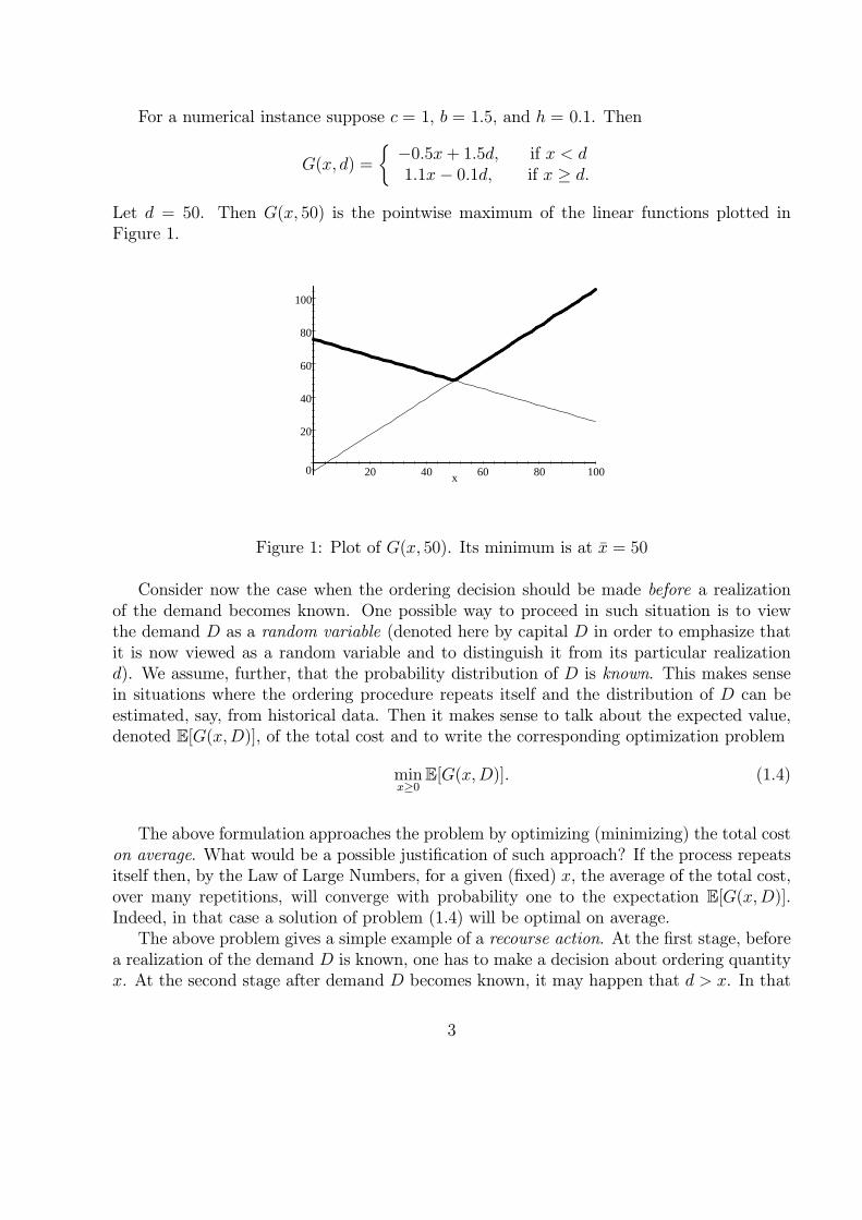
For a numerical instance suppose c = 1, b = 1.5, and h = 0.1. Then

G(x, d) =

{−0.5x+ 1.5d, if x < d1.1x− 0.1d, if x ≥ d.

Let d = 50. Then G(x, 50) is the pointwise maximum of the linear functions plotted inFigure 1.

0

20

40

60

80

100

20 40 60 80 100x

Figure 1: Plot of G(x, 50). Its minimum is at x = 50

Consider now the case when the ordering decision should be made before a realizationof the demand becomes known. One possible way to proceed in such situation is to viewthe demand D as a random variable (denoted here by capital D in order to emphasize thatit is now viewed as a random variable and to distinguish it from its particular realizationd). We assume, further, that the probability distribution of D is known. This makes sensein situations where the ordering procedure repeats itself and the distribution of D can beestimated, say, from historical data. Then it makes sense to talk about the expected value,denoted E[G(x,D)], of the total cost and to write the corresponding optimization problem

minx≥0

E[G(x,D)]. (1.4)

The above formulation approaches the problem by optimizing (minimizing) the total coston average. What would be a possible justification of such approach? If the process repeatsitself then, by the Law of Large Numbers, for a given (fixed) x, the average of the total cost,over many repetitions, will converge with probability one to the expectation E[G(x,D)].Indeed, in that case a solution of problem (1.4) will be optimal on average.

The above problem gives a simple example of a recourse action. At the first stage, beforea realization of the demand D is known, one has to make a decision about ordering quantityx. At the second stage after demand D becomes known, it may happen that d > x. In that

3

case the company can meet demand by taking the recourse action of ordering the requiredquantity d− x at a penalty cost of b > c.

The next question is how to solve the optimization problem (1.4). In the present caseproblem (1.4) can be solved in a closed form. Consider the cumulative distribution function(cdf) F (z) := Prob(D ≤ z) of the random variable D. Note that F (z) = 0 for any z < 0.This is because the demand cannot be negative. It is possible to show (see the Appendix)that

E[G(x,D)] = bE[D] + (c− b)x+ (b + h)

∫ x

0

F (z)dz. (1.5)

Therefore, by taking the derivative, with respect to x, of the right hand side of (1.5) andequating it to zero we obtain that optimal solutions of problem (1.4) are defined by theequation (b + h)F (x) + c − b = 0, and hence an optimal solution of problem (1.4) is givenby the quantile 1

x = F−1 (κ) , (1.6)

where κ := b−cb+h

.Suppose for the moment that the random variable D has a finitely supported distribu-

tion, i.e., it takes values d1, ..., dK (called scenarios) with respective probabilities p1, ..., pK.In that case its cdf F (·) is a step function with jumps of size pk at each dk, k = 1, ..., K.Formula (1.6), for an optimal solution, still holds with the corresponding κ-quantile, coin-ciding with one of the points dk, k = 1, ..., K. For example, the considered scenarios mayrepresent historical data collected over a period of time. In such case the correspondingcdf is viewed as the empirical cdf giving an approximation (estimation) of the true cdf, andthe associated κ-quantile is viewed as the sample estimate of the κ-quantile associated withthe true distribution. It is instructive to compare the quantile solution x with a solutioncorresponding to one scenario d = d, where d is, say, the mean (expected value) of D. As itwas mentioned earlier, the optimal solution of such (deterministic) problem is d. The meand can be very different from the κ-quantile x. It is also worthwhile mentioning that typicallysample quantiles are much less sensitive than the sample mean to random perturbations ofthe empirical data.

In most real settings, closed-form solutions for stochastic programming problems such as(1.4) are rarely available. In the case of finitely many scenarios it is possible to model thestochastic program as a deterministic optimization problem, by writing the expected valueE[G(x,D)] as the weighted sum:

E[G(x,D)] =K∑

k=1

pkG(x, dk). (1.7)

1Recall that, for κ ∈ (0, 1), the (left side) κ-quantile of the cumulative distribution function F (·) is definedas F−1(κ) := inf{t : F (t) ≥ κ}. In a similar way the right side κ-quantile is defined as sup{t : F (t) ≤ κ}.The set of optimal solutions of problem (1.4) is the (closed) interval with end points given by the respectiveleft and right side κ-quantiles.

4

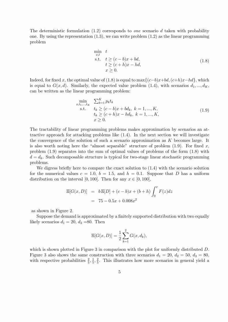
The deterministic formulation (1.2) corresponds to one scenario d taken with probabilityone. By using the representation (1.3), we can write problem (1.2) as the linear programmingproblem

minx,t

t

s.t. t ≥ (c− b)x + bd,t ≥ (c + h)x− hd,x ≥ 0.

(1.8)

Indeed, for fixed x, the optimal value of (1.8) is equal to max{(c−b)x+bd, (c+h)x−hd}, whichis equal to G(x, d). Similarly, the expected value problem (1.4), with scenarios d1, ..., dK,can be written as the linear programming problem:

minx,t1,...,tK

∑Kk=1 pktk

s.t. tk ≥ (c− b)x + bdk, k = 1, ..., K,tk ≥ (c + h)x− hdk, k = 1, ..., K,x ≥ 0.

(1.9)

The tractability of linear programming problems makes approximation by scenarios an at-tractive approach for attacking problems like (1.4). In the next section we will investigatethe convergence of the solution of such a scenario approximation as K becomes large. Itis also worth noting here the “almost separable” structure of problem (1.9). For fixed x,problem (1.9) separates into the sum of optimal values of problems of the form (1.8) withd = dk. Such decomposable structure is typical for two-stage linear stochastic programmingproblems.

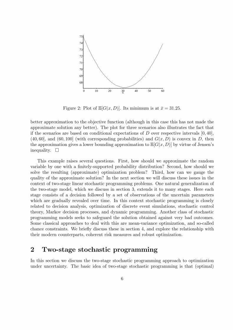
We digress briefly here to compare the exact solution to (1.4) with the scenario solutionfor the numerical values c = 1.0, b = 1.5, and h = 0.1. Suppose that D has a uniformdistribution on the interval [0, 100]. Then for any x ∈ [0, 100],

E[G(x,D)] = bE[D] + (c− b)x+ (b + h)

∫ x

0

F (z)dz

= 75− 0.5x + 0.008x2

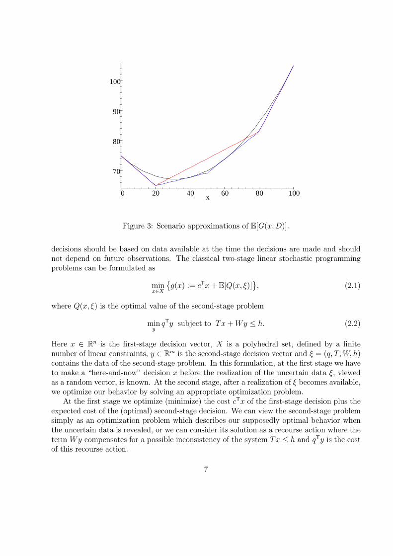
as shown in Figure 2.Suppose the demand is approximated by a finitely supported distribution with two equally

likely scenarios d1 = 20, d2 =80. Then

E[G(x,D)] =1

2

2∑

k=1

G(x, dk),

which is shown plotted in Figure 3 in comparison with the plot for uniformly distributed D.Figure 3 also shows the same construction with three scenarios d1 = 20, d2 = 50, d3 = 80,with respective probabilities 2

5, 15, 25. This illustrates how more scenarios in general yield a

5

68

69

70

71

72

73

74

75

0 10 20 30 40 50 60x

Figure 2: Plot of E[G(x,D)]. Its minimum is at x = 31.25.

better approximation to the objective function (although in this case this has not made theapproximate solution any better). The plot for three scenarios also illustrates the fact thatif the scenarios are based on conditional expectations of D over respective intervals [0, 40],(40, 60], and (60, 100] (with corresponding probabilities) and G(x,D) is convex in D, thenthe approximation gives a lower bounding approximation to E[G(x,D)] by virtue of Jensen’sinequality. �

This example raises several questions. First, how should we approximate the randomvariable by one with a finitely-supported probability distribution? Second, how should wesolve the resulting (approximate) optimization problem? Third, how can we gauge thequality of the approximate solution? In the next section we will discuss these issues in thecontext of two-stage linear stochastic programming problems. One natural generalization ofthe two-stage model, which we discuss in section 3, extends it to many stages. Here eachstage consists of a decision followed by a set of observations of the uncertain parameterswhich are gradually revealed over time. In this context stochastic programming is closelyrelated to decision analysis, optimization of discrete event simulations, stochastic controltheory, Markov decision processes, and dynamic programming. Another class of stochasticprogramming models seeks to safeguard the solution obtained against very bad outcomes.Some classical approaches to deal with this are mean-variance optimization, and so-calledchance constraints. We briefly discuss these in section 4, and explore the relationship withtheir modern counterparts, coherent risk measures and robust optimization.

2 Two-stage stochastic programming

In this section we discuss the two-stage stochastic programming approach to optimizationunder uncertainty. The basic idea of two-stage stochastic programming is that (optimal)

6

70

80

90

100

0 20 40 60 80 100x

Figure 3: Scenario approximations of E[G(x,D)].

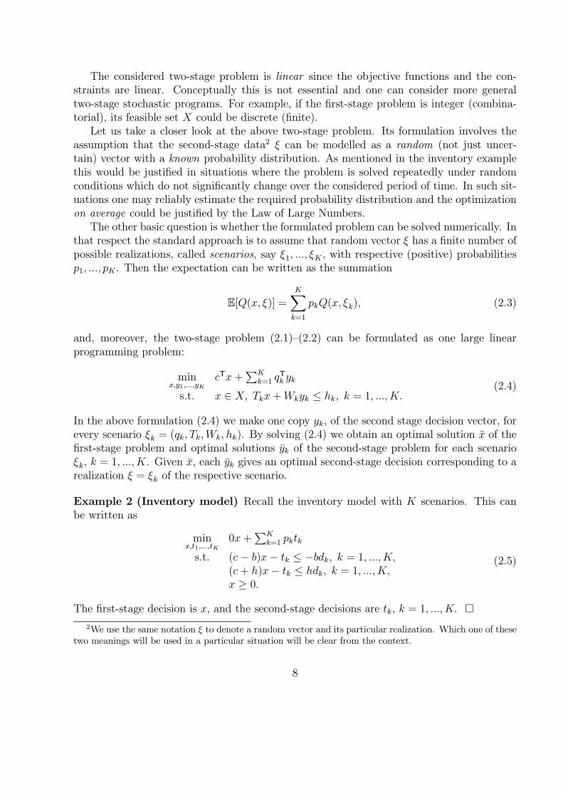
decisions should be based on data available at the time the decisions are made and shouldnot depend on future observations. The classical two-stage linear stochastic programmingproblems can be formulated as

minx∈X

{g(x) := cTx + E[Q(x, ξ)]

}, (2.1)

where Q(x, ξ) is the optimal value of the second-stage problem

miny

qTy subject to Tx + Wy ≤ h. (2.2)

Here x ∈ Rn is the first-stage decision vector, X is a polyhedral set, defined by a finitenumber of linear constraints, y ∈ Rm is the second-stage decision vector and ξ = (q, T,W, h)contains the data of the second-stage problem. In this formulation, at the first stage we haveto make a “here-and-now” decision x before the realization of the uncertain data ξ, viewedas a random vector, is known. At the second stage, after a realization of ξ becomes available,we optimize our behavior by solving an appropriate optimization problem.

At the first stage we optimize (minimize) the cost cTx of the first-stage decision plus theexpected cost of the (optimal) second-stage decision. We can view the second-stage problemsimply as an optimization problem which describes our supposedly optimal behavior whenthe uncertain data is revealed, or we can consider its solution as a recourse action where theterm Wy compensates for a possible inconsistency of the system Tx ≤ h and qTy is the costof this recourse action.

7

The considered two-stage problem is linear since the objective functions and the con-straints are linear. Conceptually this is not essential and one can consider more generaltwo-stage stochastic programs. For example, if the first-stage problem is integer (combina-torial), its feasible set X could be discrete (finite).

Let us take a closer look at the above two-stage problem. Its formulation involves theassumption that the second-stage data2 ξ can be modelled as a random (not just uncer-tain) vector with a known probability distribution. As mentioned in the inventory examplethis would be justified in situations where the problem is solved repeatedly under randomconditions which do not significantly change over the considered period of time. In such sit-uations one may reliably estimate the required probability distribution and the optimizationon average could be justified by the Law of Large Numbers.

The other basic question is whether the formulated problem can be solved numerically. Inthat respect the standard approach is to assume that random vector ξ has a finite number ofpossible realizations, called scenarios, say ξ1, ..., ξK , with respective (positive) probabilitiesp1, ..., pK . Then the expectation can be written as the summation

E[Q(x, ξ)] =K∑

k=1

pkQ(x, ξk), (2.3)

and, moreover, the two-stage problem (2.1)—(2.2) can be formulated as one large linearprogramming problem:

minx,y1,...,yK

cTx +∑K

k=1 qT

k yk

s.t. x ∈ X, Tkx+ Wkyk ≤ hk, k = 1, ..., K.(2.4)

In the above formulation (2.4) we make one copy yk, of the second stage decision vector, forevery scenario ξk = (qk, Tk,Wk, hk). By solving (2.4) we obtain an optimal solution x of thefirst-stage problem and optimal solutions yk of the second-stage problem for each scenarioξk, k = 1, ..., K. Given x, each yk gives an optimal second-stage decision corresponding to arealization ξ = ξk of the respective scenario.

Example 2 (Inventory model) Recall the inventory model with K scenarios. This canbe written as

minx,t1,...,tK

0x +∑K

k=1 pktk

s.t. (c− b)x− tk ≤ −bdk, k = 1, ..., K,(c + h)x− tk ≤ hdk, k = 1, ..., K,x ≥ 0.

(2.5)

The first-stage decision is x, and the second-stage decisions are tk, k = 1, ..., K. �

2We use the same notation ξ to denote a random vector and its particular realization. Which one of thesetwo meanings will be used in a particular situation will be clear from the context.

8

When ξ has an infinite (or very large) number of possible realizations the standard ap-proach is then to represent this distribution by scenarios. As mentioned above this approachraises three questions, namely:

1. how to construct scenarios;

2. how to solve the linear programming problem (2.4);

3. how to measure quality of the obtained solutions with respect to the ‘true’ optimum.

The answers to these questions are of course not independent: for example, the numberof scenarios constructed will affect the tractability of (2.4). We now proceed to address thefirst and third of these questions in the next subsections. The second question is not givenmuch attention here, but a brief discussion of it is given in the Notes section at the end ofthe paper.

2.1 Scenario construction

In practice it might be possible to construct scenarios by eliciting experts’ opinions on thefuture. We would like the number of constructed scenarios to be relatively modest so that theobtained linear programming problem can be solved with reasonable computational effort.It is often claimed that a solution that is optimal using only a few scenarios provides moreadaptable plans than one that assumes a single scenario only. In some cases such a claimcould be verified by a simulation. In theory, we would want some measure of guarantee thatan obtained solution solves the original problem with reasonable accuracy. We also wouldlike to point out that typically in applications only the first stage optimal solution x hasa practical value since almost certainly a “true” realization of the random (uncertain) datawill be different from the set of constructed (generated) scenarios.

A natural question for a modeler to ask is: “what is a reasonable number of scenarios tochoose so that an obtained solution will be close to the ‘true’ optimum of the original prob-

lem”. First, it is clear that this question supposes the existence of some good methodologyto construct scenarios - a poor procedure may never get close to the optimum, no matterhow many are used. If one seeks to construct scenarios, say by using experts, then it quicklybecomes clear that, as the number of random parameters increases, some automated pro-cedure to do this will become necessary. For example, suppose that the components of therandom vector ξ ∈ R

d are independent of each other and we construct scenarios by assigningto each component three possible values, by classifying future realizations as low, mediumand high. Then the total number of scenarios is K = 3d. Such exponential growth of thenumber of scenarios makes model development using expert opinion very difficult alreadyfor reasonably sized d (say d = 25).

Even assuming an automated scenario generation process, with K = 325 ≈ 1012, say,the corresponding linear program (2.4) becomes too large to be tractable. The situationbecomes even worse if we model ξi as random variables with continuous distributions. To

9

make a reasonable discretization of a (one dimensional) random variable ξi we would needconsiderably more than 3 points. At this point the modeler is faced with two somewhat con-tradictory goals. On one hand, the number of employed scenarios should be computationallymanageable. Note that reducing the number of scenarios by a factor of, say, 10 will not helpmuch if the true number of scenarios is K = 1012, say. On the other hand, the constructedapproximation should provide a reasonably accurate solution of the true problem. A possibleapproach to reconcile these two contradictory goals is by randomization. That is, scenarioscould be generated by Monte-Carlo sampling techniques.

Before we discuss the latter approach, it is important to mention boundedness and fea-sibility. The function Q(x, ξ) is defined as the optimal value of the second-stage problem(2.2). It may happen that for some feasible x ∈ X and a scenario ξk, the problem (2.2) isunbounded from below, i.e., Q(x, ξk) = −∞. This is a somewhat pathological and unrealisticsituation meaning that for such feasible x one can improve with a positive probability thesecond-stage cost indefinitely. One should make sure at the modeling stage that this doesnot happen.

Another, more serious, problem is if for some x ∈ X and scenario ξk, the system Tkx +Wky ≤ hk is incompatible, i.e., the second-stage problem is infeasible. In that case thestandard practice is to set Q(x, ξk) = +∞. That is, we impose an infinite penalty if thesecond-stage problem is infeasible and such x cannot be an optimal solution of the first-stageproblem. This will make sense if such a scenario results in a catastrophic event. It is said thatthe problem has relatively complete recourse if such infeasibility does not happen, i.e., forevery x ∈ X and every scenario ξk, the second-stage problem is feasible. It is always possibleto make the second-stage problem feasible (i.e., exhibit complete recourse) by changing it to

miny,t

qTy + γt subject to Tx + Wy − te ≤ h, t ≥ 0, (2.6)

where γ > 0 is a chosen constant and e is a vector of an appropriate dimension with allits coordinates equal to one. In this formulation the penalty for a possible infeasibility iscontrolled by the parameter γ.

2.2 Monte Carlo techniques

We now turn our attention to approaches that reduce the scenario set to a manageable sizeby using Monte Carlo simulation. That is, suppose that the total number of scenarios isvery large or even infinite. Suppose, further, that we can generate a sample ξ1, ..., ξN of Nreplications of the random vector ξ. By this we mean that each ξj , j = 1, ...,N , has the sameprobability distribution as ξ. Moreover, if ξj are distributed independently of each other, itis said that the sample is iid (independent identically distributed). Given a sample, we canapproximate the expectation function q(x) = E[Q(x, ξ)] by the average

qN (x) = N−1N∑

j=1

Q(x, ξj),

10

and consequently the “true” (expectation) problem (2.1) by the problem

minx∈X

{gN(x) := cTx +

1

N

N∑

j=1

Q(x, ξj)

}. (2.7)

This rather simple idea was suggested by different authors under different names. Inrecent literature it has became known as the sample average approximation (SAA) method.Note that for a generated sample ξ1, ..., ξN , the SAA problem (2.7) is of the same form asthe two-stage problem (2.1)—(2.2) with the scenarios ξj , j = 1, ..., N , each taken with thesame probability pj = 1/N . Note also that the SAA method is not an algorithm, one stillhas to solve the obtained SAA problem by an appropriate numerical procedure.

Example 3 (Inventory model continued) We can illustrate the SAA method on theinstance of the inventory example discussed in section 1. Recall that

G(x,D) =

{−0.5x + 1.5D, if x < D1.1x− 0.1D, if x ≥ D,

where D has a uniform distribution on [0, 100]. In Figure 4, we show SAA approximationsfor three random samples, two with N = 5 ( ξj =15, 60, 72, 78, 82, and ξj = 24, 24, 32, 41,62), and one with N = 10 (ξj = 8, 10, 21, 47, 62, 63, 75, 78, 79, 83). These samples wererandomly generated from the uniform [0, 100] distribution and rounded to integers for thesake of simplicity of presentation. The true cost function is shown in bold. �

50

60

70

80

90

100

0 20 40 60 80 100x

N=10

N=5 (sample 1)

N=5 (sample 2)

Figure 4: SAA approximations of E[G(x,D)].

11

We now can return to the question above: “how large should we choose the sample sizeN (i.e., how many scenarios should be generated) in order for the SAA problem (2.7) to givea reasonably accurate approximation of the true problem (2.1)”. Monte Carlo simulationmethods are notorious for slow convergence. For a fixed x ∈ X and an iid sample, thevariance of the sample average qN (x) is equal to Var[Q(x, ξ)]/N . This implies that, instochastic terms, the sample average converges to the corresponding expectation at a rate ofOp(N

−1/2). That is, in order to improve the accuracy by one digit, we need to increase thesample size by the factor of 100.

It should be clearly understood that it is not advantageous to use Monte Carlo techniqueswhen the number d of random variables is small. For d ≤ 2 it would be much better to usea uniform discretization grid for numerical calculations of the required integrals. This isillustrated by the example above. For d ≤ 10 quasi-Monte Carlo methods usually workbetter than Monte Carlo techniques3. The point is, however, that in principle it is notpossible to evaluate the required expectation with a high accuracy by Monte Carlo (or anyother) techniques in multivariate cases. It is also possible to show theoretically that thenumerical complexity of two-stage linear programming problems grows fast with an increaseof the number of random variables and such problems cannot be solved with a high accuracy,like say 10−4, as we expect in deterministic optimization.

The good news about Monte Carlo techniques is that the accuracy of the sample averageapproximation does not depend on the number of scenarios (which can be infinite), butdepends only on the variance of Q(x, ξ). It is remarkable and somewhat surprising that theSAA method turns out to be quite efficient for solving some classes of two-stage stochasticprogramming problems. It was shown theoretically and verified in numerical experimentsthat with a manageable sample size, the SAA method (and its variants) solves the “true”problem with a reasonable accuracy (say 1% or 2%) provided the following conditions aremet:

(i) it is possible to generate a sample of realizations of the random vector ξ,

(ii) for moderate values of the sample size it is possible to efficiently solve the obtainedSAA problem,

(iii) the true problem has relatively complete recourse,

(iv) variability of the second-stage (optimal value) function is not “too large”.

3Theoretical bounds for the error of numerical integration by quasi-Monte Carlo methods are proportionalto (logN)dN−1, i.e., are of order O

((logN)dN−1

), with the proportionality constant Ad depending on d.

For small d it is “almost” the same as of order O(N−1), which of course is better than Op(N−1/2). However,

the theoretical constant Ad grows superexponentially with increase of d. Therefore, for larger values of done often needs a very large sample size N for quasi-Monte Carlo methods to become advantageous. It isbeyond the scope of this paper to discuss these issues in detail. The interested reader may be referred to[22], for example.

12

Usually the requirement (i) does not pose a serious problem in stochastic programmingapplications, and there are standard techniques and software for generating random sam-ples. Also modern computers coupled with good algorithms can solve linear programmingproblems with millions of variables (see the Notes section at the end of the tutorial).

Condition (iii), on the other hand, requires a few words of discussion. If for some fea-sible x ∈ X the second-stage problem is infeasible with a positive probability (it does notmatter how small this positive probability is) then the expected value of Q(x, ξ), and henceits variability, is infinite. If the probability p of such an event (scenario) is very small, sayp = 10−6, then it is very difficult, or may even be impossible, to verify this by sampling. Forexample, one would need an iid sample of size N significantly bigger than p−1 to reproducesuch a scenario in the sample with a reasonable probability.

The sample average approximation problems that arise from the above process are large-scale programming problems. Since our purpose in this tutorial is to introduce stochasticprogramming models and approaches, we point to the literature for a further reading on thatsubject in the “Notes” section.

2.3 Evaluating candidate solutions

Given a feasible point x ∈ X, possibly obtained by solving a SAA problem, a practicalproblem is how to evaluate the quality of this point viewed as a candidate for solving the trueproblem. Since the point x is feasible, we clearly have that g(x) ≥ v∗, where v∗ = minx∈X g(x)is the optimal value of the true problem. The quality of x can be measured by the optimalitygap

gap(x) := g(x)− v∗.

We outline now a statistical procedure for estimating this optimality gap. The true value g(x)can be estimated by Monte Carlo sampling. That is, an iid random sample ξj, j = 1, ...,N ′,of ξ is generated and g(x) is estimated by the corresponding sample average gN ′(x) = cTx+qN ′(x). At the same time the sample variance

σ2N ′(x) :=1

N ′(N ′ − 1)

N ′∑

j=1

[Q(x, ξj)− qN ′(x)

]2, (2.8)

of qN ′(x), is calculated. Note that it is feasible here to use a relatively large sample size N ′

since calculation of the required values Q(x, ξj) involves solving only individual second-stageproblems. Then

UN ′(x) := gN ′(x) + zασN ′(x) (2.9)

gives an approximate 100(1− α)% confidence upper bound for g(x). This bound is justifiedby the Central Limit Theorem with the critical value zα = Φ−1(1−α), where Φ(z) is the cdf

13

of the standard normal distribution. For example, for α = 5% we have that zα ≈ 1.64, andfor α = 1% we have that zα ≈ 2.33.

In order to calculate a lower bound for v∗ we proceed as follows. Denote by vN theoptimal value of the SAA problem based on a sample of size N . Note that vN is a functionof the (random) sample and hence is random. To obtain a lower bound for v∗ observe thatE[gN (x)] = g(x), i.e., the sample average gN(x) is an unbiased estimator of the expectationg(x). We also have that for any x ∈ X the inequality gN(x) ≥ infx′∈X gN (x′) holds, so forany x ∈ X, we have

g(x) = E [gN(x)] ≥ E[

infx′∈X

gN (x′)

]= E [vN ] .

By taking the minimum over x ∈ X of the left hand side of the above inequality we obtainthat v∗ ≥ E[vN ].

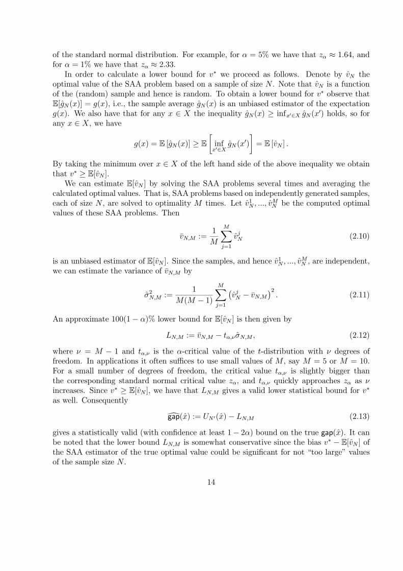
We can estimate E[vN ] by solving the SAA problems several times and averaging thecalculated optimal values. That is, SAA problems based on independently generated samples,each of size N , are solved to optimality M times. Let v1N , ..., v

MN be the computed optimal

values of these SAA problems. Then

vN,M :=1

M

M∑

j=1

vjN (2.10)

is an unbiased estimator of E[vN ]. Since the samples, and hence v1N , ..., vMN , are independent,

we can estimate the variance of vN,M by

σ2N,M :=1

M(M − 1)

M∑

j=1

(vjN − vN,M

)2. (2.11)

An approximate 100(1− α)% lower bound for E[vN ] is then given by

LN,M := vN,M − tα,νσN,M , (2.12)

where ν = M − 1 and tα,ν is the α-critical value of the t-distribution with ν degrees offreedom. In applications it often suffices to use small values of M , say M = 5 or M = 10.For a small number of degrees of freedom, the critical value tα,ν is slightly bigger thanthe corresponding standard normal critical value zα, and tα,ν quickly approaches zα as νincreases. Since v∗ ≥ E[vN ], we have that LN,M gives a valid lower statistical bound for v∗

as well. Consequently

gap(x) := UN ′(x)− LN,M (2.13)

gives a statistically valid (with confidence at least 1− 2α) bound on the true gap(x). It canbe noted that the lower bound LN,M is somewhat conservative since the bias v∗ − E[vN ] ofthe SAA estimator of the true optimal value could be significant for not “too large” valuesof the sample size N .

14

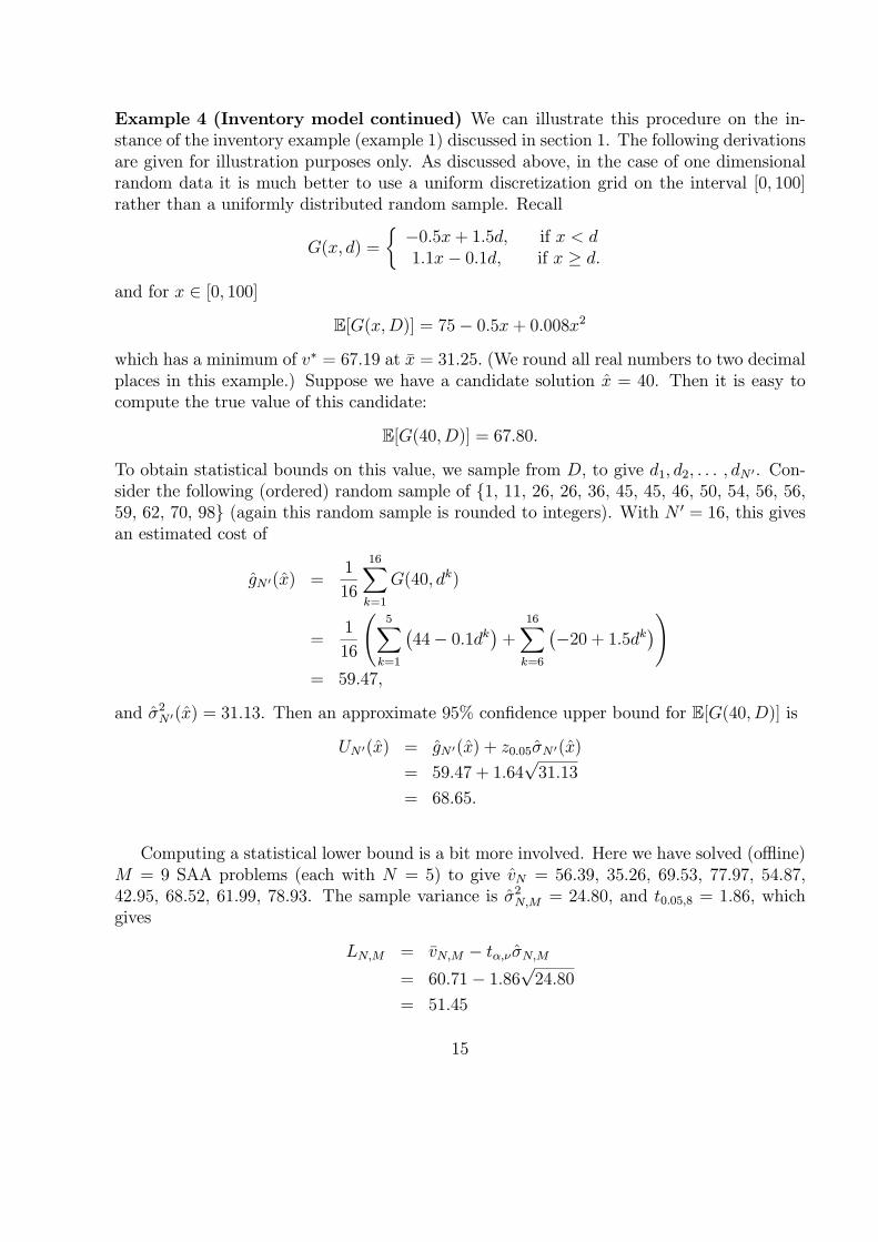
Example 4 (Inventory model continued) We can illustrate this procedure on the in-stance of the inventory example (example 1) discussed in section 1. The following derivationsare given for illustration purposes only. As discussed above, in the case of one dimensionalrandom data it is much better to use a uniform discretization grid on the interval [0, 100]rather than a uniformly distributed random sample. Recall

G(x, d) =

{−0.5x+ 1.5d, if x < d1.1x− 0.1d, if x ≥ d.

and for x ∈ [0, 100]

E[G(x,D)] = 75− 0.5x+ 0.008x2

which has a minimum of v∗ = 67.19 at x = 31.25. (We round all real numbers to two decimalplaces in this example.) Suppose we have a candidate solution x = 40. Then it is easy tocompute the true value of this candidate:

E[G(40,D)] = 67.80.

To obtain statistical bounds on this value, we sample from D, to give d1, d2, . . . , dN ′. Con-sider the following (ordered) random sample of {1, 11, 26, 26, 36, 45, 45, 46, 50, 54, 56, 56,59, 62, 70, 98} (again this random sample is rounded to integers). With N ′ = 16, this givesan estimated cost of

gN ′(x) =1

16

16∑

k=1

G(40, dk)

=1

16

(5∑

k=1

(44− 0.1dk

)+

16∑

k=6

(−20 + 1.5dk

))

= 59.47,

and σ2N ′(x) = 31.13. Then an approximate 95% confidence upper bound for E[G(40, D)] is

UN ′(x) = gN ′(x) + z0.05σN ′(x)

= 59.47 + 1.64√

31.13

= 68.65.

Computing a statistical lower bound is a bit more involved. Here we have solved (offline)M = 9 SAA problems (each with N = 5) to give vN = 56.39, 35.26, 69.53, 77.97, 54.87,42.95, 68.52, 61.99, 78.93. The sample variance is σ2N,M = 24.80, and t0.05,8 = 1.86, whichgives

LN,M = vN,M − tα,νσN,M

= 60.71− 1.86√

24.80

= 51.45

15

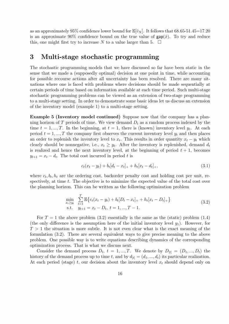
as an approximately 95% confidence lower bound for E[vN ]. It follows that 68.65-51.45=17.20is an approximate 90% confidence bound on the true value of gap(x). To try and reducethis, one might first try to increase N to a value larger than 5. �

3 Multi-stage stochastic programming

The stochastic programming models that we have discussed so far have been static in thesense that we made a (supposedly optimal) decision at one point in time, while accountingfor possible recourse actions after all uncertainty has been resolved. There are many sit-uations where one is faced with problems where decisions should be made sequentially atcertain periods of time based on information available at each time period. Such multi-stagestochastic programming problems can be viewed as an extension of two-stage programmingto a multi-stage setting. In order to demonstrate some basic ideas let us discuss an extensionof the inventory model (example 1) to a multi-stage setting.

Example 5 (Inventory model continued) Suppose now that the company has a plan-ning horizon of T periods of time. We view demand Dt as a random process indexed by thetime t = 1, ..., T . In the beginning, at t = 1, there is (known) inventory level y1. At eachperiod t = 1, ..., T the company first observes the current inventory level yt and then placesan order to replenish the inventory level to xt. This results in order quantity xt − yt whichclearly should be nonnegative, i.e., xt ≥ yt. After the inventory is replenished, demand dtis realized and hence the next inventory level, at the beginning of period t + 1, becomesyt+1 = xt − dt. The total cost incurred in period t is

ct(xt − yt) + bt[dt − xt]+ + ht[xt − dt]+, (3.1)

where ct, bt, ht are the ordering cost, backorder penalty cost and holding cost per unit, re-spectively, at time t. The objective is to minimize the expected value of the total cost overthe planning horizon. This can be written as the following optimization problem

minxt≥yt

T∑t=1

E{ct(xt − yt) + bt[Dt − xt]+ + ht[xt −Dt]+

}

s.t. yt+1 = xt −Dt, t = 1, ..., T − 1.(3.2)

For T = 1 the above problem (3.2) essentially is the same as the (static) problem (1.4)(the only difference is the assumption here of the initial inventory level y1). However, forT > 1 the situation is more subtle. It is not even clear what is the exact meaning of theformulation (3.2). There are several equivalent ways to give precise meaning to the aboveproblem. One possible way is to write equations describing dynamics of the correspondingoptimization process. That is what we discuss next.

Consider the demand process Dt, t = 1, ..., T . We denote by D[t] = (D1, ...,Dt) thehistory of the demand process up to time t, and by d[t] = (d1, ..., dt) its particular realization.At each period (stage) t, our decision about the inventory level xt should depend only on

16

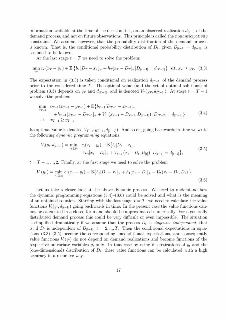
information available at the time of the decision, i.e., on an observed realization d[t−1] of thedemand process, and not on future observations. This principle is called the nonanticipativityconstraint. We assume, however, that the probability distribution of the demand processis known. That is, the conditional probability distribution of Dt, given D[t−1] = d[t−1], isassumed to be known.

At the last stage t = T we need to solve the problem:

minxT

cT (xT − yT ) + E{bT [DT − xT ]+ + hT [xT −DT ]+

∣∣D[T−1] = d[T−1]}

s.t. xT ≥ yT . (3.3)

The expectation in (3.3) is taken conditional on realization d[T−1] of the demand processprior to the considered time T . The optimal value (and the set of optimal solutions) ofproblem (3.3) depends on yT and d[T−1], and is denoted VT (yT , d[T−1]). At stage t = T − 1we solve the problem

minxT−1

cT−1(xT−1 − yT−1) + E{bT−1[DT−1 − xT−1]+

+hT−1[xT−1 −DT−1]+ + VT(xT−1 −DT−1,D[T−1]

) ∣∣D[T−2] = d[T−2]}

s.t. xT−1 ≥ yT−1.

(3.4)

Its optimal value is denoted VT−1(yT−1, d[T−2]). And so on, going backwards in time we writethe following dynamic programming equations

Vt(yt, d[t−1]) = minxt≥yt

ct(xt − yt) + E{bt[Dt − xt]+

+ht[xt −Dt]+ + Vt+1(xt −Dt,D[t]

) ∣∣D[t−1] = d[t−1]},

(3.5)

t = T − 1, ..., 2. Finally, at the first stage we need to solve the problem

V1(y1) = minx1≥y1

c1(x1 − y1) + E{b1[D1 − x1]+ + h1[x1 −D1]+ + V2 (x1 −D1,D1)

}.

(3.6)

Let us take a closer look at the above dynamic process. We need to understand howthe dynamic programming equations (3.4)—(3.6) could be solved and what is the meaningof an obtained solution. Starting with the last stage t = T , we need to calculate the valuefunctions Vt(yt, d[t−1]) going backwards in time. In the present case the value functions can-not be calculated in a closed form and should be approximated numerically. For a generallydistributed demand process this could be very difficult or even impossible. The situationis simplified dramatically if we assume that the process Dt is stagewise independent, thatis, if Dt is independent of D[t−1], t = 2, ..., T . Then the conditional expectations in equa-tions (3.3)—(3.5) become the corresponding unconditional expectations, and consequentlyvalue functions Vt(yt) do not depend on demand realizations and become functions of therespective univariate variables yt only. In that case by using discretizations of yt and the(one-dimensional) distribution of Dt, these value functions can be calculated with a highaccuracy in a recursive way.

17

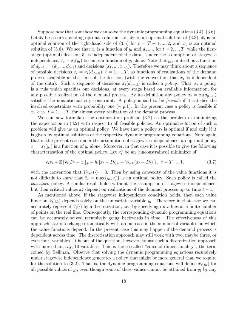
Suppose now that somehow we can solve the dynamic programming equations (3.4)—(3.6).Let xt be a corresponding optimal solution, i.e., xT is an optimal solution of (3.3), xt is anoptimal solution of the right-hand side of (3.5) for t = T − 1, ..., 2, and x1 is an optimalsolution of (3.6). We see that xt is a function of yt and d[t−1], for t = 2, ..., T , while the first-stage (optimal) decision x1 is independent of the data. Under the assumption of stagewiseindependence, xt = xt(yt) becomes a function of yt alone. Note that yt, in itself, is a functionof d[t−1] = (d1, ..., dt−1) and decisions (x1, ..., xt−1). Therefore we may think about a sequenceof possible decisions xt = xt(d[t−1]), t = 1, ..., T , as functions of realizations of the demandprocess available at the time of the decision (with the convention that x1 is independentof the data). Such a sequence of decisions xt(d[t−1]) is called a policy. That is, a policyis a rule which specifies our decisions, at every stage based on available information, forany possible realization of the demand process. By its definition any policy xt = xt(d[t−1])satisfies the nonanticipativity constraint. A policy is said to be feasible if it satisfies theinvolved constraints with probability one (w.p.1). In the present case a policy is feasible ifxt ≥ yt, t = 1, ..., T , for almost every realization of the demand process.

We can now formulate the optimization problem (3.2) as the problem of minimizingthe expectation in (3.2) with respect to all feasible policies. An optimal solution of such aproblem will give us an optimal policy. We have that a policy xt is optimal if and only if itis given by optimal solutions of the respective dynamic programming equations. Note againthat in the present case under the assumption of stagewise independence, an optimal policyxt = xt(yt) is a function of yt alone. Moreover, in that case it is possible to give the followingcharacterization of the optimal policy. Let x∗t be an (unconstrained) minimizer of

ctxt + E{bt[Dt − xt]+ + ht[xt −Dt]+ + Vt+1 (xt −Dt)

}, t = T, ..., 1, (3.7)

with the convention that VT+1(·) = 0. Then by using convexity of the value functions it isnot difficult to show that xt = max{yt, x∗t} is an optimal policy. Such policy is called thebasestock policy. A similar result holds without the assumption of stagewise independence,but then critical values x∗t depend on realizations of the demand process up to time t− 1.

As mentioned above, if the stagewise independence condition holds, then each valuefunction Vt(yt) depends solely on the univariate variable yt. Therefore in that case we canaccurately represent Vt(·) by a discretization, i.e., by specifying its values at a finite numberof points on the real line. Consequently, the corresponding dynamic programming equationscan be accurately solved recursively going backwards in time. The effectiveness of thisapproach starts to change dramatically with an increase in the number of variables on whichthe value functions depend. In the present case this may happen if the demand process isdependent across time. The discretization approach may still work with two, maybe three, oreven four, variables. It is out of the question, however, to use such a discretization approachwith more than, say, 10 variables. This is the so-called “curse of dimensionality”, the termcoined by Bellman. Observe that solving the dynamic programming equations recursivelyunder stagewise independence generates a policy that might be more general than we requirefor the solution to (3.2). That is, the dynamic programming equations will define xt(yt) forall possible values of yt, even though some of these values cannot be attained from y1 by any

18

combination of demand outcomes (d1, ..., dt−1) and decisions (x1, ..., xt−1).Stochastic programming tries to approach the problem in a different way by using a

discretization of the random process D1, ..., DT in the form of a scenario tree. That is, N1

possible realizations of the (random) demand D1 are generated. Next, conditional on everyrealization of D1, several (say the same number N2) realizations of D2 are generated, and soon. In that way N := N1× ...×NT different sample paths of the random process D1, ...,DT

are constructed. Each sample path is viewed as a scenario of a possible realization of theunderline random process. There is a large literature of how such scenario trees could (andshould) be constructed in a reasonable and meaningful way. One possible approach is touse Monte Carlo techniques to generate scenarios by conditional sampling. This leads toan extension of the SAA method to a multi-stage setting. Note that the total number ofscenarios is the product of the numbers Nt of constructed realizations at each stage. Thissuggests an explosion of the number of scenarios with increase of the number of stages.In order to handle an obtained optimization problem numerically one needs to reduce thenumber of scenarios to a manageable level. Often this results in taking Nt = 1 from a certainstage on. This means that from this stage on the nonanticipativity constraint is relaxed.

In contrast to dynamic programming, stochastic programming does not seek Vt(yt) forall values of t and yt, but focuses on computing V1(y1) and the first-stage optimal deci-sion x1 for the known inventory level y1. This makes stochastic programming more akin to adecision-tree analysis than dynamic programming (although unlike decision analysis stochas-tic programming requires the probability distributions to be independent of decisions). Apossible advantage of this approach over dynamic programming is that it might mitigatethe curse of dimensionality in situations where the states visited as the dynamic processunfolds (or the dimension of the state space) are constrained by the currently observed statey1 (whatever the actions might be). In general, however, the number of possible states thatmight be visited grows explosively with the number of stages, and so multi-stage stochasticprograms are tractable only in special cases. �

4 Risk averse optimization

In this section we discuss the problem of risk. We begin by recalling the example of thetwo-stage inventory problem.

Example 6 (Inventory model continued) Recall that

G(x,D) =

{(c− b)x + bD, if x < D,(c + h)x− hD, if x ≥ D.

We have already observed that for a particular realization of the demand D, the cost G(x, D)can be quite different from the optimal-on-average cost E[G(x, D)]. Therefore a naturalquestion is whether we can control the risk of the cost G(x,D) to be not “too high”. Forexample, for a chosen value (threshold) τ > 0, we may add to problem (1.4) the constraint

19

G(x,D) ≤ τ to be satisfied for all possible realizations of the demand D. That is, we wantto make sure that the total cost will be at most τ in all possible circumstances. Numericallythis means that the inequalities (c − b)x + bd ≤ τ and (c + h)x − hd ≤ τ should hold forall possible realizations d of the uncertain demand. That is, the ordering quantity x shouldsatisfy the following inequalities:

bd− τ

b− c≤ x ≤ hd+ τ

c + hfor all realizations d of the uncertain demand D. (4.1)

This, of course, could be quite restrictive. In particular, if there is at least one realization dgreater than τ/c, then the system (4.1) is incompatible, i.e., the corresponding problem hasno feasible solution.

In such situations it makes sense to introduce the constraint that the probability ofG(x,D) being bigger than τ is less than a specified value (significance level) α ∈ (0, 1). Thisleads to the so-called chance or probabilistic constraint which can be written in the form

Prob{G(x,D) > τ} ≤ α, (4.2)

or equivalently

Prob{G(x,D) ≤ τ} ≥ 1− α. (4.3)

By adding the chance constraint (4.2) to the optimization problem (1.4) we want to optimize(minimize) the total cost on average making sure that the risk of the cost being large (i.e.,the probability that the cost is bigger than τ) is small (i.e., less than α). We have that

Prob{G(x,D) ≤ τ} = Prob

{(c + h)x− τ

h≤ D ≤ (b− c)x + τ

b

}. (4.4)

For x ≤ τ/c the inequalities in the right hand side of (4.4) are consistent and hence for suchx,

Prob{G(x,D) ≤ τ} = F

((b− c)x + τ

b

)− F

((c + h)x− τ

h

). (4.5)

Even for small (but positive) values of α, the chance constraint (4.3) can be a significantrelaxation of the corresponding constraints (4.1).

In the numerical instance where D has uniform distribution on the interval [0, 100], andc = 1, b = 1.5, and h = 0.1, suppose τ = 99. Then τ/c = 99 is less than some realizations ofthe demand, and the system (4.1) is inconsistent. That is, there is no feasible x satisfyingconstraint G(x, d) ≤ τ for all d in the range [0, 100]. On the other hand, (4.5) becomes

Prob{G(x,D) > 99} = 1− F

(0.5x+ 99

1.5

)+ F

(1.1x− 99

0.1

)

=

1− x300− 66

100, 0 ≤ x ≤ 90,

1 + 32300

x− 1056100

, 90 < x ≤ 99,1, 99 < x < 100.

20

0

0.2

0.4

0.6

0.8

1

50 60 70 80 90 100x

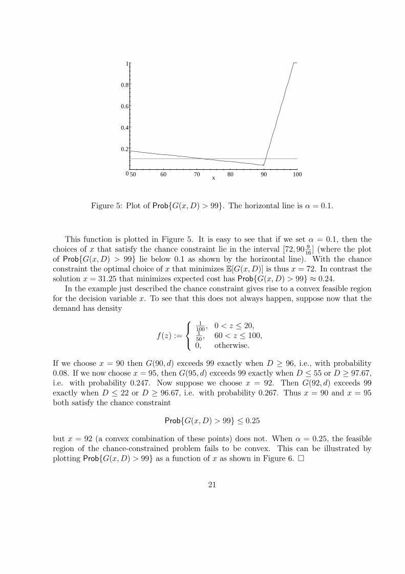
Figure 5: Plot of Prob{G(x,D) > 99}. The horizontal line is α = 0.1.

This function is plotted in Figure 5. It is easy to see that if we set α = 0.1, then thechoices of x that satisfy the chance constraint lie in the interval [72, 90 9

16] (where the plot

of Prob{G(x,D) > 99} lie below 0.1 as shown by the horizontal line). With the chanceconstraint the optimal choice of x that minimizes E[G(x,D)] is thus x = 72. In contrast thesolution x = 31.25 that minimizes expected cost has Prob{G(x,D) > 99} ≈ 0.24.

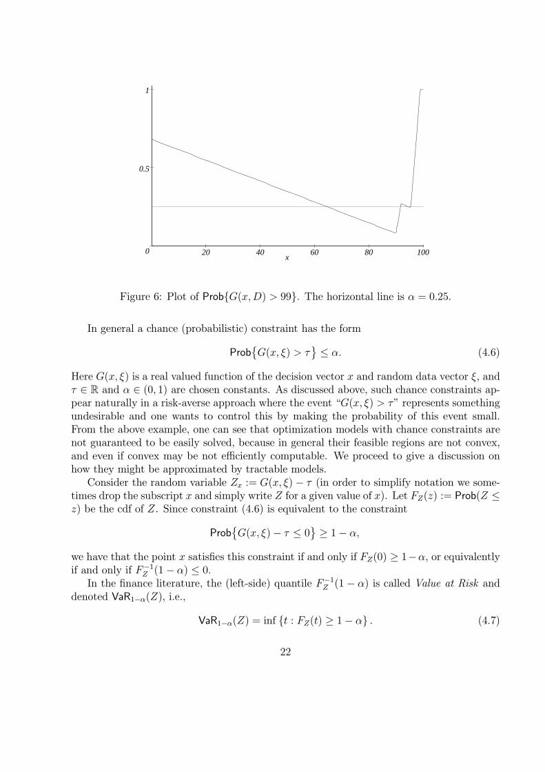
In the example just described the chance constraint gives rise to a convex feasible regionfor the decision variable x. To see that this does not always happen, suppose now that thedemand has density

f(z) :=

1100

, 0 < z ≤ 20,150, 60 < z ≤ 100,

0, otherwise.

If we choose x = 90 then G(90, d) exceeds 99 exactly when D ≥ 96, i.e., with probability0.08. If we now choose x = 95, then G(95, d) exceeds 99 exactly when D ≤ 55 or D ≥ 97.67,i.e. with probability 0.247. Now suppose we choose x = 92. Then G(92, d) exceeds 99exactly when D ≤ 22 or D ≥ 96.67, i.e. with probability 0.267. Thus x = 90 and x = 95both satisfy the chance constraint

Prob{G(x,D) > 99} ≤ 0.25

but x = 92 (a convex combination of these points) does not. When α = 0.25, the feasibleregion of the chance-constrained problem fails to be convex. This can be illustrated byplotting Prob{G(x,D) > 99} as a function of x as shown in Figure 6. �

21

0

0.5

1

20 40 60 80 100x

Figure 6: Plot of Prob{G(x,D) > 99}. The horizontal line is α = 0.25.

In general a chance (probabilistic) constraint has the form

Prob{G(x, ξ) > τ

}≤ α. (4.6)

Here G(x, ξ) is a real valued function of the decision vector x and random data vector ξ, andτ ∈ R and α ∈ (0, 1) are chosen constants. As discussed above, such chance constraints ap-pear naturally in a risk-averse approach where the event “G(x, ξ) > τ” represents somethingundesirable and one wants to control this by making the probability of this event small.From the above example, one can see that optimization models with chance constraints arenot guaranteed to be easily solved, because in general their feasible regions are not convex,and even if convex may be not efficiently computable. We proceed to give a discussion onhow they might be approximated by tractable models.

Consider the random variable Zx := G(x, ξ)− τ (in order to simplify notation we some-times drop the subscript x and simply write Z for a given value of x). Let FZ(z) := Prob(Z ≤z) be the cdf of Z. Since constraint (4.6) is equivalent to the constraint

Prob{G(x, ξ)− τ ≤ 0

}≥ 1− α,

we have that the point x satisfies this constraint if and only if FZ(0) ≥ 1−α, or equivalentlyif and only if F−1

Z (1− α) ≤ 0.In the finance literature, the (left-side) quantile F−1

Z (1− α) is called Value at Risk anddenoted VaR1−α(Z), i.e.,

VaR1−α(Z) = inf {t : FZ(t) ≥ 1− α} . (4.7)

22

Note that VaR1−α(Z + τ) = VaR1−α(Z)+ τ , and hence constraint (4.6) can be written in thefollowing equivalent form

VaR1−α[G(x, ξ)] ≤ τ . (4.8)

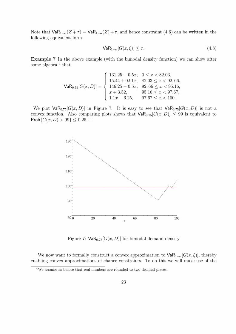
Example 7 In the above example (with the bimodal density function) we can show aftersome algebra 4 that

VaR0.75[G(x,D)] =

131.25− 0.5x, 0 ≤ x < 82.03,15.44 + 0.91x, 82.03 ≤ x < 92. 66,146.25− 0.5x, 92. 66 ≤ x < 95.16,x + 3.52, 95.16 ≤ x < 97.67,1.1x− 6.25, 97.67 ≤ x < 100.

We plot VaR0.75[G(x,D)] in Figure 7. It is easy to see that VaR0.75[G(x,D)] is not aconvex function. Also comparing plots shows that VaR0.75[G(x,D)] ≤ 99 is equivalent toProb{G(x,D) > 99} ≤ 0.25. �

80

90

100

110

120

130

0 20 40 60 80 100x

Figure 7: VaR0.75[G(x,D)] for bimodal demand density

We now want to formally construct a convex approximation to VaR1−α[G(x, ξ)], therebyenabling convex approximations of chance constraints. To do this we will make use of the

4We assume as before that real numbers are rounded to two decimal places.

23

step function

1l(z) :=

{1, if z > 0,0, if z ≤ 0.

We have that

Prob(Z > 0) = E [1l(Z)] ,

and hence constraint (4.6) can also be written as the expected value constraint:

E [1l(Zx)] ≤ α. (4.9)

As we have observed in example 7, since 1l(·) is not a convex function this operation oftenyields a nonconvex constraint, even though the function G(·, ξ) might be convex for almostevery ξ.

Let ψ : R → R be a nonnegative-valued, nondecreasing, convex function such thatψ(z) ≥ 1l(z) for all z ∈ R. By noting that 1l(tz) = 1l(z) for any t > 0, we have thatψ(tz) ≥ 1l(z) and hence the following inequality holds

inft>0E [ψ(tZ)] ≥ E [1l(Z)] . (4.10)

Consequently, the constraint

inft>0E [ψ(tZ)] ≤ α (4.11)

is a conservative approximation of the chance constraint (4.6) in the sense that the feasibleset defined by (4.11) is contained in the feasible set defined by (4.6).

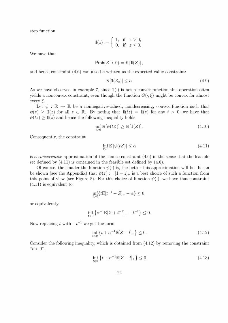
Of course, the smaller the function ψ(·) is, the better this approximation will be. It canbe shown (see the Appendix) that ψ(z) := [1 + z]+ is a best choice of such a function fromthis point of view (see Figure 8). For this choice of function ψ(·), we have that constraint(4.11) is equivalent to

inft>0{tE[t−1 + Z]+ − α} ≤ 0,

or equivalently

inft>0

{α−1E[Z + t−1]+ − t−1

}≤ 0.

Now replacing t with −t−1 we get the form:

inft<0

{t+ α−1E[Z − t]+

}≤ 0. (4.12)

Consider the following inequality, which is obtained from (4.12) by removing the constraint“t < 0”,

inft∈R

{t+ α−1E[Z − t]+

}≤ 0 (4.13)

24

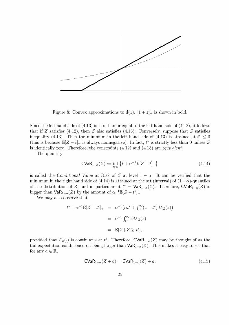
Figure 8: Convex approximations to 1l(z). [1 + z]+ is shown in bold.

Since the left hand side of (4.13) is less than or equal to the left hand side of (4.12), it followsthat if Z satisfies (4.12), then Z also satisfies (4.13). Conversely, suppose that Z satisfiesinequality (4.13). Then the minimum in the left hand side of (4.13) is attained at t∗ ≤ 0(this is because E[Z − t]+ is always nonnegative). In fact, t∗ is strictly less than 0 unless Zis identically zero. Therefore, the constraints (4.12) and (4.13) are equivalent.

The quantity

CVaR1−α(Z) := inft∈R

{t+ α−1E[Z − t]+

}(4.14)

is called the Conditional Value at Risk of Z at level 1 − α. It can be verified that theminimum in the right hand side of (4.14) is attained at the set (interval) of (1−α)-quantilesof the distribution of Z, and in particular at t∗ = VaR1−α(Z). Therefore, CVaR1−α(Z) isbigger than VaR1−α(Z) by the amount of α−1E[Z − t∗]+.

We may also observe that

t∗ + α−1E[Z − t∗]+ = α−1(αt∗ +

∫∞t∗

(z − t∗)dFZ(z))

= α−1∫∞t∗

zdFZ(z)

= E[Z | Z ≥ t∗],

provided that FZ(·) is continuous at t∗. Therefore, CVaR1−α(Z) may be thought of as thetail expectation conditioned on being larger than VaR1−α(Z). This makes it easy to see thatfor any a ∈ R,

CVaR1−α(Z + a) = CVaR1−α(Z) + a. (4.15)

25

Therefore, the constraint

CVaR1−α[G(x, ξ)] ≤ τ (4.16)

is equivalent to the constraint (4.12) and gives a conservative approximation of the chanceconstraint (4.6) (recall that (4.6) is equivalent to (4.8)). Also by the above analysis we havethat (4.16) is the best possible convex conservative approximation of the chance constraint(4.6).

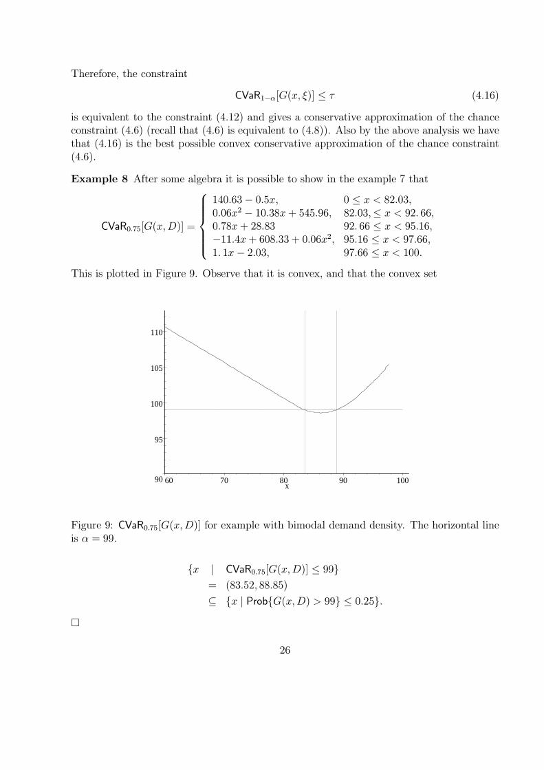
Example 8 After some algebra it is possible to show in the example 7 that

CVaR0.75[G(x,D)] =

140.63− 0.5x, 0 ≤ x < 82.03,0.06x2 − 10.38x + 545.96, 82.03,≤ x < 92. 66,0.78x + 28.83 92. 66 ≤ x < 95.16,−11.4x+ 608.33 + 0.06x2, 95.16 ≤ x < 97.66,1. 1x− 2.03, 97.66 ≤ x < 100.

This is plotted in Figure 9. Observe that it is convex, and that the convex set

90

95

100

105

110

60 70 80 90 100x

Figure 9: CVaR0.75[G(x,D)] for example with bimodal demand density. The horizontal lineis α = 99.

{x | CVaR0.75[G(x,D)] ≤ 99}= (83.52, 88.85)

⊆ {x | Prob{G(x,D) > 99} ≤ 0.25}.

�

26

The function ρ(Z) := CVaR1−α(Z) has the following properties.

(i) It is convex, i.e., if Z1 and Z2 are two random variables and t ∈ [0, 1], then

ρ (tZ1 + (1− t)Z2) ≤ tρ(Z1) + (1− t)ρ(Z2).

(ii) It is monotone, i.e., if Z1 and Z2 are two random variables such that with probabilityone Z2 ≥ Z1, then ρ(Z2) ≥ ρ(Z1).

(iii) It is positively homogeneous, i.e., if Z is a random variable and t > 0, then ρ(tZ) =tρ(Z).

(iv) It has the (translation equivariance) property: ρ(Z + a) = ρ(Z) + a for any a ∈ R.

Functions ρ(Z), defined on a space of random variables, satisfying properties (i)—(iv) werecalled coherent risk measures in [2]. Properties (i) and (ii) ensure that if G(·, ξ) is convex foralmost every ξ, then the function f(x) := ρ(G(x, ξ)) is also convex. That is, coherent riskmeasures, and in particular CVaR, preserve convexity of G(·, ξ). This property is of crucialimportance for the efficiency of numerical procedures.

Now let us consider the following optimization problem

minx∈X

E[G(x, ξ)] subject to CVaR1−α[G(x, ξ)] ≤ τ . (4.17)

Suppose that the set X is convex and for almost every ξ the function G(·, ξ) is convex. Forexample, in the case of two-stage linear programming with recourse we can take G(x, ξ) :=cTx+ Q(x, ξ). By the above discussion, it follows that the problem (4.17) is convex. Understandard regularity conditions we have that problem (4.17) is equivalent to the problem

minx∈X

{g(x) := E[G(x, ξ)] + λCVaR1−α[G(x, ξ)]

}, (4.18)

where λ ≥ 0 is an optimal solution of the dual problem. By using definition (4.14) ofCVaR1−α, we can write problem (4.18) in the form

minx∈X, t∈R

E[Hξ(x, t)], (4.19)

where

Hξ(x, t) := G(x, ξ) + λt+ λα−1[G(x, ξ)− t]+.

By using the equality [a]+ = a + [−a]+ it is straightforward to verify that

t+ α−1[Z − t]+ = [t− Z]+ + κ[Z − t]+ + Z,

where κ := α−1 − 1. Consequently

Hξ(x, t) = (1 + λ)(G(x, ξ) + γ[t−G(x, ξ)]+ + γκ[G(x, ξ)− t]+

),

27

where γ := λ/(λ + 1). Note that γ ∈ [0, 1) and κ > 0.The computational complexity of problem (4.19) is almost the same as that of the ex-

pected value problem:

minx∈X

E[G(x, ξ)]. (4.20)

The function Hξ(·, ·) is convex if G(·, ξ) is convex, and is piecewise linear if G(·, ξ) is piecewiselinear. If both these conditions hold, X is a polyhedral set, and ξ has a finite number ofrealizations then (4.19) can be formulated as a linear program.

The additional term in (4.18), as compared with (4.20), has the following interpretation.For a random variable Z define

Dκ[Z] := inft∈RE {[t− Z]+ + κ[Z − t]+} . (4.21)

Note that the minimum in the right hand side of (4.21) is attained at the quantile t∗ =VaR κ

1+κ(Z), and observe that κ/(1 + κ) = 1 − α. We can view Dκ[Z] as an (asymmetric)

measure of dispersion of Z around its (1− α)-quantile. We obtain that problem (4.19), andhence problem (4.18), are equivalent to the problem

minx∈X

{E[G(x, ξ)] + γDκ[G(x, ξ)]} . (4.22)

It is possible to give yet another interpretation for the problem (4.22). Let Z = Z(ξ)be a random variable defined on a probability space (Ξ,F , P ). We have the following dualrepresentation of the coherent risk measure ρ(Z) = E[Z] + γDκ[Z]:

ρ(Z) = supF∈A

EF [Z], (4.23)

where A is a set of probability distributions on (Ξ,F) such that

F ∈ A iff (1− γ)P (A) ≤ F (A) ≤ (1 + γκ)P (A) for any A ∈ F .

In particular, if the set Ξ = {ξ1, ..., ξK} is finite with probability distribution P defined byprobabilities p1, ..., pK, then a probability distribution p′1, ..., p

′K on Ξ belongs to A iff

(1− γ)pk ≤ p′k ≤ (1 + γκ)pk, k = 1, ...,K.

Consequently, problem (4.22) can be written in the following minimax form

minx∈X

supF∈A

EF [G(x, ξ)]. (4.24)

In the terminology of robust optimization, the set A can be viewed as an uncertainty set

for the probability distributions and problem (4.24) as the worst-case-probability stochasticprogram.

28

A popular traditional approach to controlling risk in optimization is to try to reduce vari-ability of the (random) cost G(x, ξ), and hence to make it closer to its average (expectation)E[G(x, ξ)]. In classical statistics, variability of a random variable Z is usually measured byits variance or standard deviation. This suggests adding the constraint Var[G(x, ξ)] ≤ ϑ toproblem (1.4), for some chosen constant ϑ > 0. Note that this constraint is equivalent to thecorresponding constraint

√Var[G(x, ξ)] ≤

√ϑ for the standard deviation of the total cost.

There are, however, several problems with this approach. Firstly, constraining eitherthe variance or standard deviation of G(x, ξ) means that the obtained constraint set isnot guaranteed to be convex unless G(x, ξ) is linear in x. Secondly variance and standarddeviation are both symmetrical measures of variability, and, in the minimization case, we arenot concerned if the cost is small; we just don’t want it to be too large. This motivates the useof asymmetrical measures of variability (like the coherent risk measure ρ(Z) = E[Z]+γDκ[Z])which appropriately penalize large values of the cost G(x, ξ). The following example showsthat the symmetry of variance and standard deviation is problematic even if the cost functionis linear.

Example 9 Suppose that the space Ξ = {ξ1, ξ2} consists of two points with associatedprobabilities p and 1− p, for some p ∈ (0, 1). Consider dispersion measure D[Z], defined onthe space of functions (random variables) Z : Ξ→ R, either of the form

D[Z] :=√

Var[Z] or D[Z] := Var[Z],

and the corresponding ρ(Z) := E[Z] + λD[Z]. Consider functions Z1, Z2 : Ξ→ R defined byZ1(ξ1) = −a and Z1(ξ2) = 0, where a is some positive number, and Z2(ξ1) = Z2(ξ2) = 0.Now, for D[Z] =

√Var[Z], we have that ρ(Z2) = 0 and ρ(Z1) = −pa + λa

√p(1− p). It

follows that for any λ > 0 and p < (1 + λ−2)−1 we have that ρ(Z1) > ρ(Z2). Similarly, forD[Z] = Var[Z] we have that ρ(Z1) > ρ(Z2) if a > λ−1 and p < [1 − (λa)−1]−1. That is,although Z2 dominates Z1 in the sense that Z2(ξ) ≥ Z1(ξ) for every possible realization ofξ ∈ Ξ, we have here that ρ(Z1) > ρ(Z2), i.e., ρ(·) is not monotone.

Consider now the optimization problem

minx∈R2

ρ[G(x, ξ)] s.t. x1 + x2 = 1, x1 ≥ 0, x2 ≥ 0, (4.25)

with G(x, ξ) = x1Z1(ξ) + x2Z2(ξ). Let x := (1, 0) and x∗ := (0, 1). We have here thatG(x, ξ) = x1Z1(ξ), and hence G(x, ξ) is dominated by G(x, ξ) for any feasible point x ofproblem (4.25) and any realization ξ ∈ Ξ. And yet x is not an optimal solution of thecorresponding optimization (minimization) problem since ρ[G(x, ξ)] = ρ[Z1] is greater thanρ[G(x∗, ξ)] = ρ(Z2).�

5 Notes

The inventory model, introduced in example 1 (also called the Newsvendor Problem) isclassical. This model, and its multistage extensions, are discussed extensively in Zipkin [37],to which the interested reader is referred for a further reading on that topic.

29

The concept of two-stage linear stochastic programming with recourse was introduced inBeale [4] and Dantzig [8]. Although two-stage linear stochastic programs are often regardedas the classical stochastic programming modeling paradigm, the discipline of stochastic pro-gramming has grown and broadened to cover a wide range of models and solution approaches.Applications are widespread, from finance to fisheries management. There is a number ofbooks and monographs where theory and applications of stochastic programming is dis-cussed. In that respect we can mention, for example, monographs [6, 26, 30, 36]. Chanceconstraints problems were introduced in Charnes, Cooper and Symonds [7]. For a thoroughdiscussion and development of that concept we may refer to Prekopa [26]. An introductorytreatment is available in the on-line tutorial by Henrion [12].

Questions of how to construct scenarios and to measure quality of obtained solutions havebeen studied extensively in the stochastic programming literature. A way of reducing thenumber of scenarios by certain aggregations techniques are discussed in Heitsch and Romisch[11] and Pflug [25], for example. The approach to statistical validation of a candidatesolution, discussed in section 2.3, was suggested in Norkin, Pflug and Ruszczynski [23], anddeveloped in Mak, Morton and Wood [17]. For a more recent work in that direction seeBayraksan and Morton [3].

The first mathematical discussion of risk aversion (using utility functions) is often at-tributed to Daniel Bernouilli [5]. The concept of utility was formally defined and expoundedby von Neumann and Morgenstern [21]. The idea of using a mean-variance approach tostochastic optimization goes back to Markowitz [18]. Coherent risk measures were first in-troduced by Artzner et al [2]. A discussion of drawbacks of using variance or standarddeviation as measures of dispersion in stochastic programming can be found in Takriti andAhmed [33], for example. The approach of using CVaR for approximating chance constraintsis due to Rockafellar and Uryasev [27]. We follow Nemirovski and Shapiro [20] to showthat the CVaR approximation is the best convex approximation of a chance constraint. Itis also suggested in [20] to use the exponential function ψ(z) = ez, instead of the piecewiselinear function [1 + z]+, for constructing convex conservative approximations, which has thepotential advantage of treating the obtained constraints analytically.

The term “sample average approximation” method was coined in Kleywegt et al [15],although this approach was used long before that paper under various names. Statisticalproperties of the SAA method are discussed in Shapiro [31] and complexity of two andmulti-stage stochastic programming in Shapiro and Nemirovski [32]. From a deterministicpoint of view, complexity of two-stage linear stochastic programming is discussed in Dyerand Stougie [9]. Rates of convergence of Monte Carlo and Quasi-Monte Carlo estimates ofthe expected values are discussed in Niederreiter [22]. Numerical experiments with the SAAmethod are reported in [16, 17, 35], for example.

The sample average approximation problems that arise from the sampling process of two(and multi) stage linear stochastic programs are large-scale linear programming problems.These can be attacked directly using commercial optimization software which is widely avail-able (see e.g. [10]). As the problems grow in size (with the number of scenarios) they becometoo large to solve using general-purpose codes. Of course for astronomically large numbers of

30

scenarios we cannot hope to solve any problem exactly, but at the boundary of tractabilityof general purpose codes we can exploit the special structure inherent in the formulation(2.4) to solve problems in a reasonable amount of time.

The mathematical programming literature on exploiting structure to solve large-scalelinear programs is extensive. Since our purpose in this tutorial is to introduce stochasticprogramming models and approaches to readers, we give below only a brief (and selective)overview of this body of work. A more comprehensive picture is available in the monographs[6, 30, 14].

The formulation (2.4) has a structure that lends itself to the decomposition techniquesdeveloped to solve large-scale linear programming problems. These include variants of Ben-ders decomposition (also called the L-shaped method [34]), Lagrangian and augmented La-grangian decomposition ([28],[19]) interior-point methods [29], and operator splitting [24].

The SAA approach to solving stochastic linear programs may require the solution of asequence of problems with increasing numbers of scenarios (e.g. if the error in the solutionfrom the current SAA is deemed to be too large). In this case it makes sense to use informa-tion obtained in the solution of the problem to guide the solution to a larger SAA problem.This is the approach adopted by so-called internal sampling methods, e.g., the stochasticdecomposition method developed by Higle and Sen [13].

When some or all of the decision variables must take integer values, the formulation (2.4)becomes an integer linear program, which in general lacks the convexity properties to enabledecomposition techniques. To overcome this, stochastic integer programs are attacked usinga variety of techniques that combine advances in large-scale integer programming with thespecial structure that arises in applications. A more comprehensive discussion of this isprovided in the online tutorial by Ahmed [1].

It should be clearly understood that simple examples given in this paper are for illus-tration purposes only. It could be dangerous to make general conclusions based on suchsimple examples. Our intuition based on an analysis of one-dimensional models could bequite misleading in higher dimensional cases.

6 Appendix

6.1 Derivation of (1.5)

Recall

G(x,D) = cx + bmax{D − x, 0}+ hmax{x−D, 0}. (6.1)

Let g(x) = E[G(x,D)]. It is a convex continuous function. For x ≥ 0 we have

g(x) = g(0) +

∫ x

0

g′(z)dz,

31

where at nondifferentiable points the derivative g′(z) is understood as the right hand sidederivative. Since D ≥ 0 we have that g(0) = bE[D]. Also observe that

d

dxE[max{D − x, 0}] = Prob(D ≥ x)

and

d

dxE[max{x−D, 0}] = Prob(D ≤ x)

so

g′(z) = c + ddzE [bmax{D − z, 0}+ hmax{z −D, 0}]

= c− bProb(D ≥ z) + hProb(D ≤ z)= c− b(1− F (z)) + hF (z)= c− b + (b + h)F (z).

Thus

E[G(x,D)] = bE[D] + (c− b)x+ (b + h)

∫ x

0

F (z)dz. (6.2)

6.2 Derivation of best convex approximation to chance constraints.

Let ψ : R → R be a nonnegative valued, nondecreasing, convex function such that ψ(z) ≥1l(z) for all z ∈ R, and ψ(0) = 1. Since ψ is convex, it is supported, at 0, by a linearfunction, i.e., there is a ∈ R such that ψ(z) ≥ 1 + az for all z ∈ R. Moreover, since ψ(z)is nondecreasing, it follows that a ≥ 0. If a = 0, then ψ(z) ≥ 1 of course. So suppose thata > 0. Then since ψ(z) is nonnegative, we have that ψ(z) ≥ max{0, 1 + az} = [1 + az]+ forall z. Note now that the function ψ is defined up to a scaling, i.e., the basic inequality (4.10)is invariant with respect to rescaling t �→ at. It follows that ψ(z) := [1 + z]+ is a minimalvalue (and hence a best) choice of such function ψ.

AcknowledgementsThe authors would like to thank David Morton, Maarten van der Vlerk, and BernardoPagnoncelli for helpful comments on an earlier version of this tutorial.

References

[1] Ahmed, S., Introduction to stochastic integer programming, http://www.stoprog.org.

[2] Artzner, P. Delbaen, F., Eber, J.-M. and Heath, D., Coherent measures of risk, Mathe-matical Finance, 9, 203—228 (1999).

32

[3] Bayraksan, G. and Morton, D., Assessing solution quality in stochastic programs, Math-ematical Programming, 108, 495—514 (2006).

[4] Beale, E.M.L., On minimizing a convex function subject to linear inequalities, Journalof the Royal Statistical Society, Series B, 17, 173—184 (1955).

[5] Bernouilli, D., Exposition of a new theory on the measurement of risk, 1738. (Translatedby L. Sommer in Econometrica 22 (1): 22-36, 1954)

[6] Birge, J.R. and Louveaux, F., Introduction to Stochastic Programming, Springer, 1997.

[7] Charnes, A., Cooper, W.W. and G.H. Symonds, Cost horizons and certainty equivalents:an approach to stochastic programming of heating oil, Management Science, 4, 235—263(1958).

[8] Dantzig, G.B., Linear programming under uncertainty,Management Science, 1, 197—206(1955).

[9] Dyer, M. and Stougie, L., Computational complexity of stochastic programming prob-lems, Mathematical Programming, 106, 423—432 (2006).

[10] Fourer, R., Linear programming frequently asked questions, http://www-unix.mcs.anl.gov/otc/Guide/faq/linear-programming-faq.html (2000).

[11] Heitsch, H. and Romisch,W. Scenario reduction algorithms in stochastic programming,Computational Optimization and Applications, 24, 187-206 (2003).

[12] Henrion, R., Introduction to chance-constrained programming, http://www.stoprog.org.

[13] Higle, J.L. and Sen, S. Stochastic Decomposition: A Statistical Method for Large Scale

Stochastic Linear Programming, Kluwer Academic Publishers, Dordrecht, 1996.

[14] Kall, P. and Meyer, J., Stochastic Linear Programming, Models, Theory, and Compu-tation. Springer, 2005.

[15] Kleywegt, A. J., Shapiro, A. and Homem-de-Mello, T., The sample average approxima-tion method for stochastic discrete optimization, SIAM J. Optimization, 12, 479-502(2001).

[16] Linderoth, J., Shapiro, A. and Wright, S., The empirical behavior of sampling methodsfor stochastic programming, Annals of Operations Research, 142, 215-241 (2006).

[17] Mak, W.K., Morton, D.P. and Wood, R.K., Monte Carlo bounding techniques for deter-mining solution quality in stochastic programs, Operations Research Letters, 24, 47—56(1999).

[18] Markowitz, H.M., Portfolio selection, Journal of Finance, 7, 77—91 (1952).

33

[19] Mulvey, J.M. and Ruszczynski, A., A new scenario decomposition method for large-scalestochastic optimization, Operations Research, 43, 477—490 (1995).

[20] Nemirovski, A. and Shapiro, A., Convex approximations of chance constrained pro-grams, SIAM J. Optimization, 17, 969-996 (2006).

[21] von Neumann, J. and Morgenstern, O., Theory of Games and Economic Behavior, 1944.

[22] Niederreiter, H., Random Number Generation and Quasi-Monte Carlo Methods, SIAM,Philadelphia, 1992.

[23] Norkin, V.I., Pflug, G.Ch. and Ruszczynski, A., A branch and bound method forstochastic global optimization. Mathematical Programming, 83, 425—450 (1998).

[24] Pennanen, T. and Kallio, M. A splitting method for stochastic programs, Annals ofOperations Research, 142, 259-268 (2006).

[25] Pflug, G.Ch., Scenario tree generation for multiperiod financial optimization by optimaldiscretization. Mathematical Programming B, 89, 251-271 (2001).

[26] Prekopa, A., Stochastic Programming, Kluwer, Dordrecht, Boston, 1995.

[27] Rockafellar, R.T. and Uryasev, S.P., Optimization of conditional value-at-risk, TheJournal of Risk, 2, 21-41 (2000).

[28] Rockafellar, R.T. and Wets, R.J-B., Scenarios and policy aggregation in optimizationunder uncertainty, Mathematics of Operations Research, 16, 119-147 (1991).

[29] Ruszczynski, A., Interior point methods in stochastic programming, IIASA Workingpaper WP-93-8, (1993).

[30] Ruszczynski, A. and Shapiro, A., (Eds.), Stochastic Programming, Handbook in OR &MS, Vol. 10, North-Holland Publishing Company, Amsterdam, 2003.

[31] Shapiro, A., Monte Carlo sampling methods, in: Ruszczynski, A. and Shapiro, A.,(Eds.), Stochastic Programming, Handbook in OR & MS, Vol. 10, North-Holland Pub-lishing Company, Amsterdam, 2003.

[32] Shapiro, A. and Nemirovski, A., On complexity of stochastic programming problems, in:Continuous Optimization: Current Trends and Applications, pp. 111-144, V. Jeyakumarand A.M. Rubinov (Eds.), Springer, 2005.

[33] Takriti, S. and Ahmed, S., On robust optimization of two-stage systems, MathematicalProgramming, 99, 109-126 (2004).

[34] Van Slyke, R. and Wets, R.J-B., L-shaped linear programs with applications to optimalcontrol and stochastic programming, SIAM J. on Appl. Math., 17, 638-663 (1969).

34

[35] Verweij, B., Ahmed, S., Kleywegt, A.J., Nemhauser, G. and Shapiro, A., The sampleaverage approximation method applied to stochastic routing problems: a computationalstudy, Computational Optimization and Applications, 24, 289—333 (2003).

[36] Ziemba, W.T. and Wallace, S.W., Applications of Stochastic Programming, SIAM, 2006.

[37] Zipkin, P.H. Foundations of Inventory Management, McGraw-Hill, 2000.

35