a two dimensional euler flow solver on adaptive cartesian grids
TRANSCRIPT

A TWO DIMENSIONAL EULER FLOW SOLVER ON ADAPTIVE CARTESIAN
GRIDS
A THESIS SUBMITTED TO THE GRADUATE SCHOOL OF NATURAL AND APPLIED SCIENCES
OF MIDDLE EAST TECHNICAL UNIVERSITY
BY
BERCAN SİYAHHAN
IN PARTIAL FULFILLMENT OF THE REQUIREMENTS FOR
THE DEGREE OF MASTER OF SCIENCE IN
MECHANICAL ENGINEERING
MAY 2008

Approval of the Thesis:
A TWO DIMENSIONAL EULER FLOW SOLVER ON ADAPTIVE
CARTESIAN GRIDS
submitted by BERCAN SİYAHHAN in partial fulfilment of the requirements for the degree of Master of Science in Mechanical Engineering Department, Middle East Technical University by,
Prof. Dr. Canan Özgen _______________ Dean, Graduate School of Natural and Applied Sciences Prof. Dr. S. Kemal İder _______________ Head of Department, Mechanical Engineering Prof. Dr. M. Haluk Aksel _______________ Supervisor, Mechanical Engineering Dept., METU Assist. Prof. Dr. Cüneyt Sert _______________ Co-Supervisor, Mechanical Engineering Dept., METU
Examining Committee Members:
Prof. Dr. Kahraman Albayrak _______________ Mechanical Engineering Dept., METU Prof. Dr. M. Haluk Aksel _______________ Mechanical Engineering Dept., METU Assist. Prof. Dr. Cüneyt Sert _______________ Mechanical Engineering Dept., METU Prof. Dr. İsmail H. Tuncer _______________ Aerospace Engineering Dept., METU Instructor Dr. Tahsin Çetinkaya _______________ Mechanical Engineering Dept., METU Date: 02/05/2008

iii
I hereby declare that all information in this document has been obtained and presented in accordance with academic rules and ethical conduct. I also declare that, as required by these rules and conduct, I have fully cited and referenced all material and results that are not original to this work.
Name, Last name : Bercan Siyahhan
Signature :

iv
ABSTRACT
A TWO DIMENSIONAL EULER FLOW SOLVER ON ADAPTIVE CARTESIAN GRIDS
Siyahhan, Bercan
M.S., Department of Mechanical Engineering
Supervisor: Prof. Dr. M. Haluk Aksel
Co-Supervisor: Assist. Prof. Dr. Cüneyt Sert
May 2008, 121 pages
In the thesis work, a code to solve the two dimensional compressible Euler equations
for external flows around arbitrary geometries have been developed. A Cartesian
mesh generator is incorporated to the solver. Hence the pre-processing can be
performed together with the solution within a single code. The code is written in the
C++ programming language and its object oriented capabilities have been exploited
to save memory in the data structure developed.
The Cartesian mesh is formed by dividing squares successively into its four
quadrants. The main advantage of using this type of a mesh is the ability to generate
meshes around geometries of arbitrary complexity quickly and to adapt the mesh
easily based on the solution. The main disadvantage of this method is that the
treatment of the cells that are cut by the geometry.
For the solution procedure Roe’s method as well as flux vector splitting methods are
used for the flux evaluation. The flux vector splitting schemes used are van Leer,
AUSM, AUSMD and AUSMV methods. Time discretization is performed using a

v
multi-stage method. To increase the accuracy least squares reconstruction is
employed.
The code is validated by performing calculations around a NACA0012 airfoil profile.
The effect of reconstruction is demonstrated by plotting the pressure coefficient on
the airfoil. The distribution obtained using reconstruction is very close to the
experimental one while there is a considerable deviation for the case without
reconstruction. Also the shock capturing capabilities of different methods have been
investigated. In addition the performance of each method is analyzed for flow around
an NLR 7301 airfoil with a flap.
Keywords: Cartesian Mesh Generation, Approximate Riemann Solver of Roe, Euler
Equations, Solution Refinement, Flux Vector Splitting

vi
ÖZ
UYARLAMALI KARTEZYEN AĞLARDA İKİ BOYUTLU EULER AKIŞ ÇÖZÜCÜSÜ
Siyahhan, Bercan
Yüksek Lisans, Makina Mühendisliği Bölümü
Tez Yöneticisi: Prof. Dr. M. Haluk Aksel
Ortak Tez Yöneticisi: Yard. Doç. Dr. Cüneyt Sert
Mayıs 2008, 121 sayfa
Bu tez çalışması kapsamında, herhangi bir geometri etrafındaki iki boyutlu
sıkıştırılabilir dış akışları Euler denklemlerinin çözümüyle modellemek için bir kod
yazılmıştır. Çözücüye bir Kartezyen ağ çözücüsü ilave edilmiştir. Böylece hem ağ
oluşturma hem de çözüm işlemlerinin aynı kodla yapılması sağlanmıştır. Kod C++
dilinin nesneye yönelik programlama özellikleriyle veri yapısının kullandığı hafızayı
azlatma amacı güdülerek yazılmıştır.
Kartezyen hesaplama ağı karelerin art arda dörde bölünmesiyle oluşturulmaktadır.
Kartezyen ağların temel artısı değişik karmaşıklıktaki geometriler etrafında hızla ağ
oluşturulabilmesi ve çözüme göre ağın uyarlanabilmesidir. Temel eksisi ise geometri
tarafından kesilen hücrelerin ele alınmasındaki zorluktur.
Çözümde hücre akılarını bulmak için Roe’nun metodunun yanı sıra FVS metodları
da kullanılmaktadır. FVS metodlarından van Leer, AUSM, AUSMD ve AUSMV
kullanılmaktadır. Daha sonra zamanda integrasyon için çok aşamalı bir metod
kullanılmaktadır. Yöntemin doğruluğunu artırmak için hücre içinde akış değişkenleri
yeniden yapılandırılmaktadır.

vii
Yöntemin geçerliliği NACA0012 kanat profili etrafındaki akış çözülerek sınanmıştır.
Yeniden yapılandırmanın etkileri kanat üzerindeki basınç katsayılarının çizilmesiyle
vurgulanmaktadır. Yeniden yapılandırmalı dağılım deneysel dağılıma yakındır ancak
yeniden yapılandırma olmadan elde edilen sonuçlar deneyselden ciddi farklılıklar
göstermektedir. Ayrıca farklı metodların şok yakalama özellikleri de sınanmıştır.
Farklı metodların performansları NLR7301 profili etrafındaki akış çözülerek de
kıyaslanmaktadır.
Anahtar Kelimeler: Kartezyen Ağ Oluşturucusu, Roe’nun Yaklaşık Riemann
Çözücüsü, Euler Denklemleri, Yeniden Yapılandırma, Çözüm Uyarlamalı Ağ

viii
Dedicated to my family

ix
ACKNOWLEDGEMENTS
I would like to thank my supervisor Prof. Dr. Haluk Aksel, co-supervisor Asst. Prof.
Dr. Cüneyt Sert and Dr. Ruhşen Çete for their assistance, support and constructive
criticisms during my thesis work.
I would also like to thank Emre Gürdamar, Çağrı Şişman, Doruk Özdemir, Güneş
Nakiboğlu and Mehtap Çakmak with whom I had the pleasure of having fruitful
discussions.
Also I would like to express my appreciation for the company of Ender Özden and
Samet Özkan with whom I have shared the same work environment.
Last but not least I would like to express my gratitude for all individuals and
institutions that realize and cherish knowledge as something to be shared openly and
freely.

x
TABLE OF CONTENTS
ABSTRACT ................................................................................................................ iv
ÖZ ............................................................................................................................... vi
ACKNOWLEDGEMENTS ........................................................................................ ix
TABLE OF CONTENTS ............................................................................................. x
LIST OF TABLES .................................................................................................... xiv
LIST OF FIGURES ................................................................................................... xv
LIST OF SYMBOLS ................................................................................................ xix
CHAPTERS
1. INTRODUCTION.................................................................................................... 1
1.1 Overview of Computational Fluid Dynamics (CFD) ................................... 1
1.2 Main Elements of a CFD Program ............................................................... 2
1.3 Mesh Generation .......................................................................................... 3
1.3.1 Structured Meshes .................................................................................. 3
1.3.2 Unstructured Meshes .............................................................................. 4
1.3.2.1 Triangular Unstructured Meshes .................................................... 4

xi
1.3.2.2 Cartesian Meshes ............................................................................ 6
1.4 Solution Methods ......................................................................................... 7
1.4.1 Finite Difference Method ....................................................................... 7
1.4.2 Finite Element Method ........................................................................... 7
1.4.3 Finite Volume Method ........................................................................... 8
1.5 Assessment of the Solution Methods ........................................................... 9
2. DATA STRUCTURE & MESH GENERATION ................................................. 10
2.1 Data Structure............................................................................................. 10
2.1.1 Terminology for the Cartesian Cells .................................................... 10
2.1.2 Neighbour Cell Procedures .................................................................. 12
2.1.3 Information for Cut and Computational Cells ..................................... 13
2.2 Clipping Procedure .................................................................................... 16
2.2.1 Comparison of Polygon and Line Clipping Algorithms ...................... 16
2.2.2 Liang-Barsky Line Clipping Algorithm ............................................... 17
2.3 Mesh Generation ........................................................................................ 21
2.3.1 Uniform Mesh Generation ................................................................... 21
2.3.2 Box Adaptation & Cell-types ............................................................... 25
2.3.2.1 Regular Cut-cells .......................................................................... 28

xii
2.3.2.2 Irregular Cut-cells ......................................................................... 31
2.3.2.2.1 Concave-Split ........................................................................... 32
2.3.2.2.2 Convex-United ......................................................................... 35
2.3.3 Curvature Adaptation ........................................................................... 37
3. NUMERICAL METHOD ...................................................................................... 40
3.1 Governing Equations .................................................................................. 40
3.2 One Dimensional Riemann Problem for Linear Systems .......................... 42
3.3 The Approximate Riemann Solver of Roe ................................................. 47
3.3.1 Solution Algorithm .............................................................................. 54
3.4 Flux Vector Splitting .................................................................................. 56
3.4.1 Van Leer Flux Vector Splitting ............................................................ 57
3.4.2 AUSM (Liou-Steffen) Flux Vector Splitting ....................................... 58
3.4.3 AUSMD Flux Vector Splitting ............................................................ 59
3.4.4 AUSMV Flux Vector Splitting ............................................................ 61
3.5 Boundary Conditions ................................................................................. 61
3.6 Reconstruction of the Flow Variables ........................................................ 62
3.6.1 Gauss-Green Reconstruction ................................................................ 63
3.6.2 Least Squares (Minimum Energy) Reconstruction .............................. 64

xiii
3.6.3 Gradient Limiting ................................................................................. 67
3.7 Temporal Discretization ............................................................................. 68
3.7.1 Explicit Time Stepping Schemes ......................................................... 68
3.7.2 Determination of the Time Step ........................................................... 70
3.8 Solution Refinement .................................................................................. 71
4. RESULTS & DISCUSSIONS ............................................................................... 72
4.1 NACA0012 ................................................................................................ 72
4.1.1 Subsonic Tests ...................................................................................... 72
4.1.2 Transonic Tests .................................................................................... 81
4.2 NLR 7301 with Flap .................................................................................. 88
5. CONCLUSIONS .................................................................................................. 106
BIBLIOGRAPHY .................................................................................................... 109
APPENDICES
A. COORDINATES OF NACA0012 ...................................................................... 113
B. COORDINATES OF NLR 7301 & FLAP .......................................................... 116

xiv
LIST OF TABLES
TABLES
Table 2. 1- Information stored for different types of cells ......................................... 15
Table 3.1- Stage coefficients and CFL numbers for the multi-stage method ............ 69
Table 4.1- Comparison of first and second order solutions ....................................... 78
Table 4.2- Computational characteristics of the methods for evaluating fluxes ........ 84
Table 4.3- Computational performance of the methods for NLR 7301 AoA 6˚ ........ 92
Table 4.4- Computational performance of the methods for NLR 7301 AoA 10.1˚ ... 95
Table 4.5- Computational performance of the methods for NLR 7301 AoA 13.1˚ ... 98
Table A.1- Coordinates of NACA0012 Profile ........................................................ 113
Table B.1- The coordinates of NLR 7301 ................................................................ 116
Table B.2- The coordinates of flap .......................................................................... 119

xv
LIST OF FIGURES
FIGURES
Figure 1.1- The stages of the advancing front method ................................................ 5
Figure 1.2- Vornoї diagram for the grid points ............................................................ 6
Figure 2.1- The relation between cells ....................................................................... 11
Figure 2.2- The tree structure ..................................................................................... 11
Figure 2.3- Neighbours of a cell ................................................................................ 12
Figure 2.4- The visible and invisible regions for a clipping window ........................ 18
Figure 2.5- Automatically known neighbours of a cell ............................................. 23
Figure 2.6- Neighbours associated with the parent cell’s edge neighbours ............... 24
Figure 2.7- Imaginary boxes around a three element airfoil ...................................... 26
Figure 2.8- Mesh around the slat and the airfoil ........................................................ 27
Figure 2.9- Naming convention of a cell ................................................................... 28
Figure 2.10- Examples of regular cut-cells ................................................................ 30
Figure 2.11- Grouping and treatment of irregular cut-cells ....................................... 32
Figure 2.12- Conversion of an irregular cut-cell ........................................................ 33

xvi
Figure 2.13- Concave-split to special subgroup of regular cut-cells conversion ....... 34
Figure 2.14- Concave-split to regular cut-cells conversion ....................................... 35
Figure 2.15- Convex-united to inside cells conversion .............................................. 36
Figure 2.16- Convex-united to regular cut-cells conversion ...................................... 36
Figure 2.17- The normals of two neighbouring cut-cells ........................................... 38
Figure 2.18- Calculation of the normal ...................................................................... 38
Figure 3.1- Solution of a 1-D Riemann problem for a set of linear equations ........... 44
Figure 3.2- Graphical interpretation of flux vector splitting ...................................... 57
Figure 3.3- Ghost right state at the solid wall ............................................................ 62
Figure 3.4- Region formed by the support set............................................................ 64
Figure 4.1- Cp vs. chord for first order solution ........................................................ 73
Figure 4.2- Cp vs. chord for second order solution ................................................... 74
Figure 4.3- A refined and non-refined mesh around stagnation point ....................... 75
Figure 4.4- Comparison of the second order solutions .............................................. 76
Figure 4.5- Mach contours for NACA0012 subsonic flow ........................................ 77
Figure 4.6- Lift coefficient vs. angle of attack graph ................................................. 79
Figure 4.7- Residual plot for first and second order solutions ................................... 80
xvii
Figure 4.8- Pressure coefficient vs. chord graph for the AUSM methods ................. 82
Figure 4.9- Pressure coefficient vs. chord graph for Roe, van Leer and AUSMV .... 83
Figure 4.10- Residual plot for transonic flow ............................................................ 85
Figure 4.11- Effect of refinement at shock location .................................................. 86
Figure 4.12- Effect of refinement around stagnation point ........................................ 86
Figure 4.13- Mach contours for transonic flow around NACA0012 airfoil .............. 87
Figure 4.14- Pressure coefficient vs. chord for AUSMV with and without refinement
.................................................................................................................................... 88
Figure 4.15- Definition of geometry variables for NLR 7301 with flap .................... 89
Figure 4.16- Pressure coefficient vs. chord graph (AUSM methods AoA 6˚) ........... 90
Figure 4.17- Pressure coefficient vs. chord graph (AUSM, Roe, van Leer AoA 6˚) . 91
Figure 4.18- Pressure coefficient vs. chord graph (AUSM methods AoA 10.1˚) ...... 93
Figure 4.19- Pressure coefficient vs. chord graph (AUSM, Roe, van Leer AoA 10.1˚)
.................................................................................................................................... 94
Figure 4.20- Pressure coefficient vs. chord graph (AUSM methods AoA 13.1˚) ...... 96
Figure 4.21- Pressure coefficient vs. chord graph (AUSM, Roe, van Leer AoA 13.1˚)
.................................................................................................................................... 97
Figure 4.22- Effect of solution refinement around stagnation region of NLR 7301.. 99
Figure 4.23- Effect of solution refinement around the flap ....................................... 99

xviii
Figure 4.24- Pressure coefficient vs. chord for van Leer AoA 6˚ ............................ 100
Figure 4.25- Pressure coefficient vs. chord for van Leer AoA 10.1˚ ....................... 101
Figure 4.26- Pressure coefficient vs. chord for van Leer AoA 13.1˚ ....................... 102
Figure 4.27- Flow field for NLR 7301 with flap AoA 6˚ ........................................ 103
Figure 4.28- Flow field for NLR 7301 with flap AoA 10.1˚ ................................... 103
Figure 4.29- Flow field for NLR 7301 with flap AoA 13.1˚ ................................... 104

xix
LIST OF SYMBOLS
U: vector of conserved variables
U :vector of rotated conserved variables F(U): flux vector function ˆ ˆ( )F U : rotated flux vector function
F : flux vector dV: volume element dA: surface area element n : face normal t: time Acell: area of a cell
s∆ : length of cell face ρ : density u : velocity in the x-direction v : velocity in the y-direction
th : total enthalpy
p : pressure ρ : Roe averaged density u : Roe averaged velocity in the x-direction v : Roe averaged velocity in the y-direction
th : Roe averaged total enthalpy
p : Roe averaged pressure
te : total energy
u : normal velocity v : tangential velocity γ : specific heat ratio a : speed of sound V : velocity a : Roe averaged speed of sound V : Roe averaged velocity
α : angle of attack T : temperature M : Mach number R : gas constant T : transformation matrix A : Jacobian of the flux vector V : vector of characteristic variables λ : eigenvalue of the Jacobian matrix
( )Av u :averaging function Φ : gradient limiter R : residual function β : stage coefficients σ : CFL number Ψ : convective spectral radius S : length of projection Subscripts c : value at centroid with th R : right state variable L : left state variable stag : stagnation condition inf : free stream x : derivative in x component y: derivative in x component Superscripts ~ : Roe averaged quantity ˆ : components in normal-tangential coordinates T : transpose - : averaged quantity max : maximum value min: minimum value x: component in the x-direction y: component in the y-direction

1
CHAPTER 1
INTRODUCTION
In this thesis, numerical methods are employed to resolve external flows around
arbitrary geometries. The thesis work consists of generating a Cartesian mesh around
the input geometry, solving the Euler equations numerically with the finite volume
method for the desired flow quantities and obtaining the necessary aerodynamic
forces to verify the solution. To understand the motivation for choosing the methods
followed, a brief introduction must be made to mesh generation and solution
techniques employed in the field of computational fluid dynamics (CFD).
1.1 Overview of Computational Fluid Dynamics (CFD)
Computational fluid dynamics is a branch of fluid dynamics which employs
numerical methods for solving the equations of fluid flow which are impossible to
solve analytically due to their complex nature. Hence CFD is the third approach for
solving a flow problem alongside analytical and experimental methods.
It can be said that emergence of CFD as a tool for solving flow problems has taken
place only in the mid 1900s so it is a relatively new field of study compared to
analytical and experimental methods. Since the publication of Isaac Newton’s
Principia in 1687, theoretical and experimental methods, often combined, were the
only tools for analyzing fluid flows of differing nature (1). With the development of
digital computers, however, CFD has become an indispensible tool in the field of
fluid dynamics, arguably with the pioneering work of Kopal who in 1947 formed
tables for the supersonic flow over sharp cones after solving the governing equations
numerically. In the 1950s and 1960s CFD, has been applied to re-entry problems and

2
has established its place among the three essential methods for analyzing a fluid flow
problem (1).
1.2 Main Elements of a CFD Program
Any CFD program mainly consists of three parts; the pre-processor, the solver and
the post-processor (2) .
The pre-processor gathers the inputs to the problem being analyzed, the fluid
properties, boundary conditions, geometry around which the fluid flow will be
investigated. Also the grid is generated around the input geometry by the pre-
processor.
The solver part of the program uses numerical techniques to resolve the flow around
the input geometry. This is accomplished by converting the governing partial
differential methods to algebraic set of equations in the three conventional finite
difference, finite element and finite volume methods.
The post-processor is the part where the solution obtained is visualized. Contours of
desired scalars and the vector fields are displayed within the domain of interest. Also
non-dimensional variables and physical quantities of interest are calculated so as to
verify the solution and to judge whether the mesh generated and the schemes used
are appropriate for the problem at hand.
The program developed in the scope of the thesis work contains a pre-processor
which gathers the inputs of the problem and generates a Cartesian mesh in the
computational domain and a solver which uses the finite volume method for the
solution of the compressible Euler equations in the conserved form. The mesh
generation and different solution methods will be discussed in some detail below. For
the post-processor a commercially available program Tecplot and a freely distributed
program Mayavi have been used.

3
1.3 Mesh Generation
Mesh generation is the most time consuming and the most crucial step in obtaining a
solution to a fluid flow problem. The generated mesh should comply with
requirements of the solution schemes to be used in order to get accurate results.
In general, there are two types of meshes; the structured and the unstructured meshes.
Each one of these two types of meshes can then be classified further according to the
method used to construct them.
1.3.1 Structured Meshes
A mesh is considered to be structured if the organization of the grid points and the
form of the grid cells depend on a general mathematical rule instead of their position
(3). In other words, the grid points can be arranged as a regular array as (i, j, k) with
the neighbouring point being known as (i, j, k+1) (4). Hence the connectivity of the
grid points to form the cells is implicitly implied by the general mathematical rule.
The structured grids can be classified further according to the technique used to
generate them as algebraic, elliptic and hyperbolic grids. The algebraic grids are
formed simply by transforming cells in a Cartesian computational domain to a
physical domain to obtain a boundary conforming mesh, the elliptic grids are
obtained as a result of solving an elliptic differential equation to obtain a mesh that
satisfies the Laplace equations while for the hyperbolic grids are obtained by solving
hyperbolic equations (4).
The advantages of structured meshes are that they are boundary conforming so by
adjusting the grid spacing, meshes for viscous solutions can be obtained. They
require less data storage since the connectivity information is implicitly known.
One disadvantage of the structured meshes is that they require more computation
power, since the governing partial differential equations or the algebraic rules must
be solved and computations must be performed for the transformations from the

4
computational to physical spaces. However the most important disadvantage of the
structured meshes is that they cannot easily be applied to complex geometries that
are formed by more than one body that have small clearances or are not well
streamlined.
1.3.2 Unstructured Meshes
If the grid points cannot be arranged as a regular array and additional information is
required for the connectivity of the grid points then the mesh is unstructured. The
unstructured meshes, though they can comprise of elements of any shape, are formed
of triangular or rectangular elements generally in the two-dimensional case.
The advantages of the unstructured meshes are that they can be applied to geometries
of arbitrary complexity with ease, they are more suitable to automatic meshing, and
no transformation between a computational and a physical domain will be needed.
While the disadvantage of these meshes is that they require more complex data
structures for storing the connectivity of grid points and the neighbour cell
information.
1.3.2.1 Triangular Unstructured Meshes
The most widely used methods for forming triangular unstructured meshes are the
advancing front and the Delaunay triangulation methods.
In the advancing front method, the points are added to the ones that represent the
geometry as the mesh is created. The added points are connected to already existing
points to form triangles. Then, the points that are available for triangle formation
termed as the front are connected to newly added points to update the front until the
whole domain is meshed (4). In this approach, extensive search algorithms must be
employed when adding new grid points to ensure that the newly formed cells adjust
to the existing ones. Also, the closing stage of this approach, where the front folds

5
over itself, introduces some difficulties (3). An example of the advancing front
method is illustrated in Figure 1.1.
Figure 1.1- The stages of the advancing front method
The other and may be the most popular triangular meshing procedure, Delaunay
triangulation, requires points to be created before the meshing process and is closely
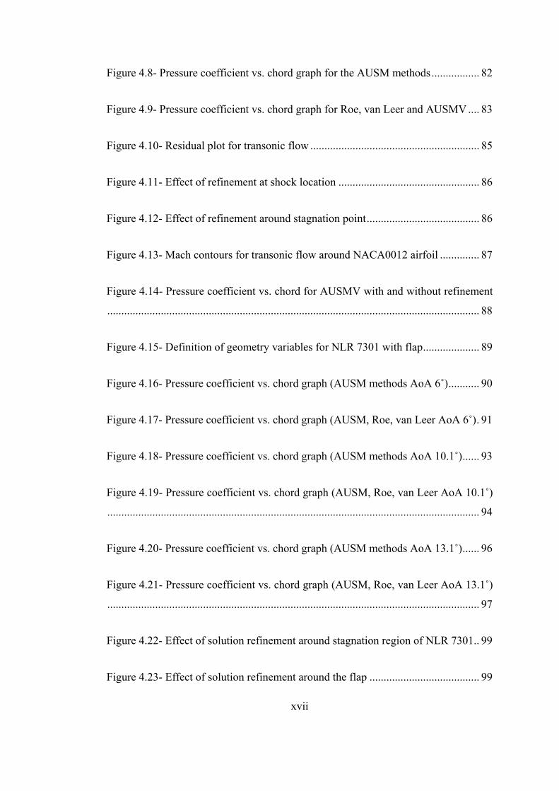
linked to the concept of Vornoї diagrams. The Vornoї diagram is obtained by
tessellating the domain into Vornoї regions which are regions that are closer to one
particular point within the domain than the others. This is illustrated in Figure 1.2.
Hence they can be obtained by the perpendicular bisectors of the lines between
neighbouring points. Once the diagram is formed, any points that have a Vornoї edge
between them are connected to form the triangular mesh. The circum-circles of the
triangular elements do not contain any other point in the domain and the resulting
mesh is unique for the point distribution. This method is suitable for mesh adaptation
since for a newly added point, the Vornoї diagram is updated locally and new
triangles are formed.
6
Figure 1.2- Vornoї diagram for the grid points
1.3.2.2 Cartesian Meshes
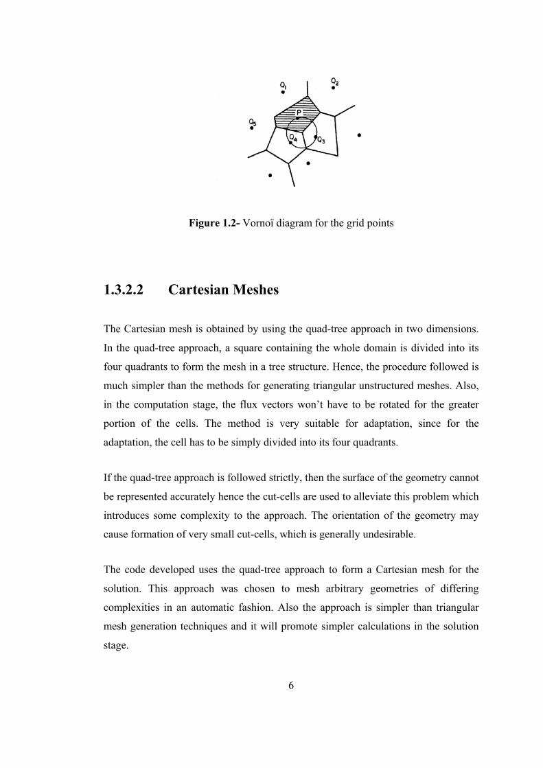
The Cartesian mesh is obtained by using the quad-tree approach in two dimensions.
In the quad-tree approach, a square containing the whole domain is divided into its
four quadrants to form the mesh in a tree structure. Hence, the procedure followed is
much simpler than the methods for generating triangular unstructured meshes. Also,
in the computation stage, the flux vectors won’t have to be rotated for the greater
portion of the cells. The method is very suitable for adaptation, since for the
adaptation, the cell has to be simply divided into its four quadrants.
If the quad-tree approach is followed strictly, then the surface of the geometry cannot
be represented accurately hence the cut-cells are used to alleviate this problem which
introduces some complexity to the approach. The orientation of the geometry may
cause formation of very small cut-cells, which is generally undesirable.
The code developed uses the quad-tree approach to form a Cartesian mesh for the
solution. This approach was chosen to mesh arbitrary geometries of differing
complexities in an automatic fashion. Also the approach is simpler than triangular
mesh generation techniques and it will promote simpler calculations in the solution
stage.

7
1.4 Solution Methods
The partial differential equations governing the flow of a fluid must be discretised in
order to convert them into algebraic equations and get a numerical solution. The
most widely used methods for the discretisation of the governing equations are the
finite difference, finite element and finite volume methods.
1.4.1 Finite Difference Method
The finite difference method is based on the differential form of the governing
system of partial differential equations. The derivatives of the conserved quantities
appearing in these equations are approximated by differences of these unknown
quantities at neighbouring grid points. These differences are derived from the Taylor
series and their order of accuracy is dependent on the number of points used in the
difference equation. Once the difference equations are written in terms of unknown
quantities, these algebraic equations can be solved numerically with the boundary
conditions to obtain the value of the conserved quantities at each grid point.
The major setback of this method is that it requires a regular structured mesh in order
to express the derivatives accurately (5). Hence, the method is not very suitable for
unstructured meshes or cases where the geometry is complex.
1.4.2 Finite Element Method
The finite element method which was initially developed for structural problems
from 1940s through 1960s, divides the computational domain into triangular or
rectangular sub-domains and represents the variation of the unknown quantities in
terms of piecewise continuous functions. Then the unknown coefficients of these
functions are found by establishing algebraic equations through satisfying the
governing equations in a weighted residual form over each element (6).

8
The finite element method, with its mathematical background being functional
analysis, has been investigated by mathematicians since its development for
engineering purposes, and is a very rigorous method with specific conditions for
existence and convergence criteria and exactly derived error bounds.
Even though this method is very well established in structural mechanics, it is still in
the stages of evolution for complex flow problems such as compressible flows
governed by Euler or Navier-Stokes equations (1).
1.4.3 Finite Volume Method
The finite volume method which was first devised as a special form of the finite
difference method in the 1970s uses the integral form of the governing equations of a
fluid flow. There is a wide range of methods for discretising the convective and
diffusive terms of the governing integral equations as well as the definition of the
control volumes for which the governing equations are satisfied. More specifically it
is possible to store the flow variables at the centroid of the cells for a cell centred
approach, or at the vertices for a cell vertex formulation. Another possibility is to
have a staggered grid where the scalar quantities and different vector quantities can
be stored on overlaid cells as in the Semi-Implicit Method for Pressure-Linked
Equations (SIMPLE) algorithm (2). Hence the method has a considerable inherent
flexibility (5). Also, since the method is directly based on the governing integral
equations, the basic concepts of the different schemes are more comprehensible than
the finite element method (2). This property of the finite volume method promotes
development of numerical schemes based on physics of the flow. Approximate
Riemann methods, which are used for evaluating the convective terms is one
example. One other advantage of the method is with the direct discretisation of the
governing integral equations, conservation of mass, momentum and energy will be
guaranteed at a discrete level (5).

9
In the code developed, cell centred finite volume method has been used with of
Roe’s approximate Riemann method for the evaluation of the convective fluxes
through the cell surfaces as well as the flux vector splitting schemes.
1.5 Assessment of the Solution Methods
Theoretically, a numerical solution will tend to the exact solution if infinite number
of cells is used. Since this is not reasonable, a numerical scheme must possess the
conservativeness, boundedness and transportiveness properties (2). The
conservativeness property states that flux leaving through a certain face of a cell
must enter the adjacent cell. The boundedness of a solution guarantees that numerical
errors introduced by the discretisation of the governing equations will not prevent
convergence. This property is related to the stability of the discretisation scheme
used. The stability of a scheme can be analyzed by the discrete perturbation analysis
or the von Neumann stability analysis (7). Finally, the transportiveness of numerical
scheme deals with the directionality of the solution. For example, the solution of a
flow dominated by convection will depend more on the upwind direction, hence
upwind schemes will be more appropriate; whereas for a flow that is diffusive, a non-
directional central method will be more appropriate.

10
CHAPTER 2
DATA STRUCTURE & MESH GENERATION
2.1 Data Structure
In the code developed, a Cartesian unstructured mesh is generated around the input
geometry. Since an unstructured mesh is used, the first step in the mesh generation is
to construct an appropriate data structure that will store the necessary data for each
cell in the domain. However before describing each variable that is stored, the
terminology adopted must be explained.
2.1.1 Terminology for the Cartesian Cells
The mesh is obtained by dividing squares successively, starting from a single large
square, by connecting the midpoints of opposing edges until the desired resolution is
obtained. This process results in a tree structure. The large square comprising the
outer boundary of the domain is termed as the root cell. A cell (square) is called the
parent of its four quadrant cells which form as a result of division and the four
quadrant cells are called the children of the parent cell in turn. The children cells are
numbered according to the quadrant they occupy. A cell without any children is
called a leaf cell. The leaf cells can also be called the computational cells since the
actual calculations for the field variables are performed for these cells. These
concepts are illustrated below in Figure 2.1.

11
Figure 2.1- The relation between cells
Among the computational cells, some are cut by geometry lines and these are called
cut-cells. The other cells mainly serve the purpose of traversing the tree. Also there is
a level concept associated with each one of the cells. The level of the four children of
a cell is one higher than that of their parent. The root cell is assigned a level of zero.
The tree structure associated with the structure shown in Figure 2.1 is illustrated in
Figure 2.2 to exemplify some of the concepts defined above.
Figure 2.2- The tree structure
child 1
child 1 child 2 child 4child 3
child 3
child 1 child 2 child 4 child 3
child 2 child 4
root level 0
level 1
level 2
leaf cells
child1 child 2
child 3 child 4
leaf cell parent

12
2.1.2 Neighbour Cell Procedures
As was mentioned before for unstructured meshes the neighbours must also be stored
since for the calculation of the fluxes through a face, the neighbour along that edge
must be known. Also the neighbours will be used to determine the variation of the
conserved variables within the cells.
A cell will have four neighbours along its edges called the edge neighbours. These
neighbours are named east, west, north and south according to the edge they are
associated with. Also computational cells will have four neighbours through their
vertices named as vertex neighbours; northeast, southeast, northwest, southwest. The
general rule for the mesh is that a cell can have neighbours of levels that are one
degree different than the cell. This ensures the grid smoothness and also simplifies
flux calculations through the faces. If a neighbour is at the same level or one lower
level, then it will be recognized as the neighbour along the corresponding edge, but if
it is at one higher level the neighbour’s parent will be recognized instead of having
two neighbours along the edge. Figure 2.3 illustrates the concepts related to
neighbouring relations and also the possible configurations that might occur for a
cell.
Figure 2.3- Neighbours of a cell
no northeastnorth neighbour
east neighbour west neighbour
south neighbour southeast neighbour
northwest neighbour
southwest neighbour
S1 S2 SE
y
x

13
In Figure 2.3 the east, west and southwest neighbours of the cell are at the same level
while the north and northwest neighbours are at one lower level. These cells are
recognized as the neighbours themselves meanwhile the parent of the cells marked as
S1, S2 and SE are recognized as the south and southeast neighbours respectively.
Since the north neighbour is at a lower level the north and northeast neighbours are
identical in which case the cell is considered to have no northeast neighbour, hence a
vertex neighbour of a cell should be distinct if it is to be stored.
2.1.3 Information for Cut and Computational Cells
As it is defined earlier there are three types of cells; the parent cells for traversing the
tree, the computational leaf cells and the cut-cells, which are special types of
computational cells. The amount of data stored for each cell depends on its type. The
information stored for a parent cell is shared for all types of cells, while
computational cells will have additional information and for cut-cells further
additional information will be stored.
For each cell in the domain, the x and y coordinates of the centre and the level of the
cell are stored. Also there are a total of thirteen pointers pointing to other cells in the
domain. Of these thirteen pointers four point to the children of the cell, if the cell is a
leaf cell then these pointers are null pointers. Eight of the remaining nine pointers
point to the neighbours of the cell. Of these eight pointers four point to edge
neighbours, the remaining four point to the vertex neighbours and they are allocated
only for computational cells. The remaining one of the thirteen pointers points to the
parent of the cell. This pointer is null only for the root cell.
Besides the thirteen pointers aforementioned there are nine more pointers which are
allocated only for computational cells. Four of these pointers store the conserved
field variables for the continuity, momentum and energy equations. Of the remaining
five pointers two are storing the gradient and the curl of the velocity vector. One
pointer stores information dictating the cell to be refined at a stage of mesh
generation or solution adaptation. One stores coefficients that will be used in solution

14
reconstruction and the last one stores the type of the cell; whether the cell resides
totally outside or inside the geometry or whether it is cut by it.
Finally there is a set of seven pointers which are allocated for the cut-cells. Three of
these seven pointers store the x and y coordinates of the centroid and area of the cell
while two store the x and y coordinates of the end lines of the intersections of
geometry lines with the cell edges. Of the remaining two pointers one stores which
edges are cut by geometry lines while the last one stores information on which
portion of the cell’s edges flux passes through. The table below shows a summary of
the information stored for different types of cells.

15
Table 2. 1- Information stored for different types of cells
xcent:ycent:level:
child1:child2:child3:child4:eneigh:wneigh:nneigh:sneigh:parent:
ro:rouvel:rovvel:
roen:gradient:
curl:recons:refine:
celltype:neneigh:seneigh:
nwneigh:swneigh:
centx:centy:area:xcut:ycut:
edgecut:fluxcut:
pointer to first quadrant childpointer to second quadrant childpointer to third quadrant child
pointer to southeast neighbour
density associated to the cellproduct of density and velocity in the x direction associated to the cell
ALL CELLS
product of density and velocity in the y direction associated to the cellproduct of density and total energy associated to the cellpointer to gradient of velocity
pointer to fourth quadrant childpointer to east neighbourpointer to west neighbourpointer to north neighbourpointer to south neighbourpointer to parent
x coordinate of center of square containing the celly coordinate of center of square containing the celllevel of the cell
pointer to the y coordinate of cut location on edgepointer to edges cut byb the geometrypointer to the information regarding flux
COMPUTATIONAL CELLS
CUT-CELLS
pointer to northwest neighbourpointer to southwest neighbour
pointer to x coordinate of the centroid of the cellpointer to y coordinate of the centroid of the cellpointer to the area of the cellpointer to the x coordinate of cut location on edge
pointer to curl of velocitypointer toarray containing geometry based reconstruction coefficientspointer to flag for refinementpointer to the cell type (inside, outside, cut-cell)pointer to northeast neighbour

16
2.2 Clipping Procedure
Before describing the mesh generation process in detail, the procedure for
determining the location of the points cut by the input geometry for the cut-cells
must be explained.
Clipping is the process of determining the portion of a geometrical shape that resides
within a given clipping window. For the code developed, the input geometry, which
is a polygon comprising of connected line segments, is to be clipped and the clipping
windows are the computational cells within the domain. The two options for the
clipping procedure are the polygon clipping, if the input geometry is conceived as a
polygon, line clipping if the input geometry is conceived as a collection of individual
line segments.
2.2.1 Comparison of Polygon and Line Clipping Algorithms
When the polygon and line clipping algorithms are compared, in general, it is seen
that the simplest polygon clipping algorithm, Sutherland-Hodgeman (8), is not
capable of handling concave geometries effectively. However there are other
polygon clipping algorithms that can handle arbitrary geometries such as self
intersecting geometries and geometries with internal holes. Since these cases are not
in the scope of the current study, the application of these algorithms would bring
unnecessary complications. Hence, the line clipping algorithms are preferred to
polygon clipping algorithms.
After this general comparison, a few of the line clipping algorithms were compared
amongst themselves. First the Liang-Barsky (9) line clipping algorithm is compared
with the most classical algorithm, Sutherland-Cohen (10) algorithm. In the work of
Liang and Barsky (9), the performance of their algorithm was tested along with the
Sutherland-Cohen line clipping algorithm with 4 sets of data containing 1000
randomly generated line segments. To reduce the effects of random variation, each
line segment was clipped 1000 times resulting in a total of 4 million clippings. It was
17
reported that an improvement of about 36 percent in the execution time was
obtained.
Even though Liang and Barsky claim that their algorithm is more efficient than
Sutherland Cohen, other researchers postulate that experimental analysis is
inadequate to measure the performance of a clipping algorithm. Instead it is
suggested that a measurement based on operation count should be used (11). A study
conducted by J. D. Day (12) takes both the experimental and operations count view
into consideration and reveals that Nicholl-Lee-Nicholl (11), Sobkow-Pospisil-Yang
(13) algorithms are more efficient in both aspects compared to the Liang-Barsky
algorithm. However the algorithms mentioned are considerably more complex, in
fact the latter algorithm classifies lines into 81 different cases.
Since the clipping procedure will be carried out once at the mesh generation step for
all the computational cells and for the cells formed as a result of solution adaptation,
its effect on overall computation time will not be very significant. Hence, the
simplest algorithm that is the easiest to implement has been chosen. Thus the Liang-
Barsky line clipping algorithm has been employed to determine the location of the
points that are cut by the input geometry lines.
2.2.2 Liang-Barsky Line Clipping Algorithm
The Liang-Barsky line clipping algorithm (9) tests the extensions of given line
segments against each one of the four boundaries of a rectangular clipping window
independently, to determine which if any portion of the line segment is inside the
clipping window. A line segment with end points V0 and V1 which happens to reside
wholly within a clipping window is shown in Figure 2.4. The line obtained from the
segment and its extensions will be tested with each one of the lines comprising the
boundary of the clipping window to determine which portion of the line is visible.
After each test the invisible part of the line will be discarded. After all the boundaries
are tested, the portion of the line segment that is inside the clipping window will be
obtained.
18
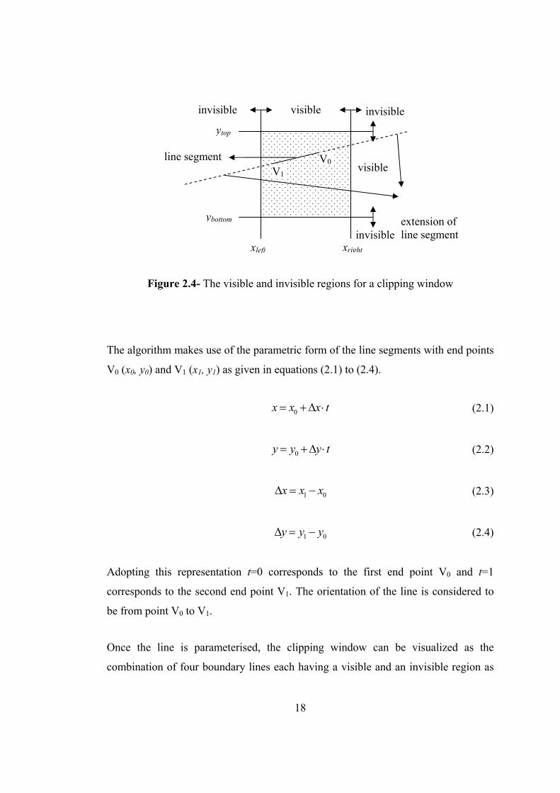
Figure 2.4- The visible and invisible regions for a clipping window
The algorithm makes use of the parametric form of the line segments with end points
V0 (x0, y0) and V1 (x1, y1) as given in equations (2.1) to (2.4).
0x x x t= +∆ ⋅ (2.1)
0y y y t= +∆ ⋅ (2.2)
1 0x x x∆ = − (2.3)
1 0y y y∆ = − (2.4)
Adopting this representation t=0 corresponds to the first end point V0 and t=1
corresponds to the second end point V1. The orientation of the line is considered to
be from point V0 to V1.
Once the line is parameterised, the clipping window can be visualized as the
combination of four boundary lines each having a visible and an invisible region as
visible
visible invisible invisible
invisiblexrightxleft
ybottom
ytop
line segment V0V1
extension of line segment

19
in Figure 2.4. Ultimately, the intersection of all the visible sides of each boundary
line would give visible region for the whole clipping window.
The visible region for the clipping window can be represented in terms of four
inequalities using the parametric relations (2.1) to (2.4).
0rightx t x x∆ ⋅ ≤ − (2.5)
0 leftx t x x−∆ ⋅ ≤ − (2.6)
0topy t y y∆ ⋅ ≤ − (2.7)
0 bottomy t y y−∆ ⋅ ≤ − (2.8)
Finally these relationships can be generalized to determine the parametric values
corresponding to the segment of the line that resides inside the clipping window.
i ip t q⋅ ≤ 1,.., 4i = (2.9)
where
1p x= ∆ 1 0rightq x x= −
2p x= −∆ 2 0 leftq x x= −
3p y= ∆ 3 0topq y y= −
4p y= −∆ 4 0 bottomq y y= −
It is observed that when pi is positive, the orientation of the extended line is from the
visible side of a particular boundary line to its invisible side. This will result in an
upper limit for the visible portion of the line.

20
i
i
qtp
≤ (2.10)
When pi is negative, the orientation of the line is from the invisible side to the visible
side, hence a lower bound for the extended line is expected.
i
i
qtp
≥ (2.11)
Since the portion of the line segment and not the extended line that resides in the
clipping window is sought another condition that the bound obtained for t should be
between 0 and 1 must also be implemented. Thus for the case when pi is different
than zero; the problem of determining the values of t for which a certain portion of
the line segment is within the clipping window becomes a min-max problem in the
form as in
0t t≥ (2.12)
1t t≤ (2.13)
where
0
1
max | 0, 1,2,3,4 , 0
min | 0, 1,2,3,4 , 1
ii
i
ii
i
qt p ip
qt p ip
⎛ ⎞⎧ ⎫= < =⎜ ⎟⎨ ⎬⎜ ⎟⎩ ⎭⎝ ⎠
⎛ ⎞⎧ ⎫= > =⎜ ⎟⎨ ⎬⎜ ⎟⎩ ⎭⎝ ⎠
The t0 and t1 values obtained as a result of this min-max problem should satisfy the
following equation
0 1 0 1t t t t t≤ ≤ ⇒ ≤ (2.14)
21
Finally, the case when pi is zero should be considered. The case pi equals to zero
corresponds to a vertical or a horizontal line. For this case a relationship independent
of t is obtained as
0 iq≤ (2.15)
The validity of this statement is solely dependent on the value of qi. If qi is positive,
the line segment is visible for that boundary line else it is invisible. This is referred to
as the trivial reject case.
2.3 Mesh Generation
The mesh generation is performed in three main steps. The first one is the uniform
mesh generation where a mesh of uniform sized elements of the desired level is
obtained. The second one is the box adaptation in which cells around an imaginary
box (rectangle) of given dimensions around the input bodies are refined till they
reach a desired size. The type of the cells; cut-cell, inside, outside, are determined at
this stage. The final step is to refine the cells around the places where there are large
gradients on the bodies. The procedure followed is similar to the one outlined in (14).
2.3.1 Uniform Mesh Generation
An initial uniform mesh is formed in the solution domain which will be refined in the
later stages to form the mesh on which the solution is to be performed. The reason
for forming this initial mesh is to have a prescribed resolution in the outer boundaries
of the domain.
Uniform mesh generation is fairly straightforward; starting from the root cell,
refinement is performed when the cell level is less than the desired level. If a cell is
to be refined, first the level of the edge and vertex neighbours must be investigated.
If a neighbour is at a lower level, then that neighbour must be refined prior to the
refinement of the cell. In this way, the one level rule is preserved in the process of
22
mesh generation. The one level rule states that the difference in the levels of two
neighbouring cells cannot exceed one. This rule enforces a smooth mesh and also
eases the calculations for the fluxes. When a cell is to be refined, it is simply divided
into its four quadrants which are its children. Then the level of the children can be set
to be one more than that of their parent and their centres can be calculated from the
centre coordinate of their parent’s, the overall size of the domain, and its level as
(2.16) to (2.19)
( / 2) ( / 2) , 2 2c parent c parentl l
d dx x y y= + = + (2.16)
( / 2) ( / 2) , 2 2c parent c parentl l
d dx x y y= − = + (2.17)
( / 2) ( / 2) , 2 2c parent c parentl l
d dx x y y= − = − (2.18)
( / 2) ( / 2) , 2 2c parent c parentl l
d dx x y y= + = − (2.19)
for the 1st quadrant to 4th quadrant children, respectively. Where d is the domain size
and l is the level of the cell.
Once this information is obtained, the neighbours of each cell must also be
determined. The procedure followed is similar to the one outlined by De Zeeuw (14).
For any cell two edge neighbours and one vertex neighbour will be known
automatically since they will be the children of the cell’s parent. The other two edge
neighbours and one vertex neighbour will be associated with the parent’s edge
neighbours while the last vertex neighbour will be related to a neighbour of a
neighbour of the parent cell. Thus, similar operations will be performed for each
group of cells.
The neighbour search can be explained in detail for a first quadrant child
exemplifying the process for the other quadrant children. For a first quadrant child,

23
the first group of neighbours, ones known automatically, will be the west, south and
southwest neighbours. They are the second, fourth and the third quadrant children of
the cell’s parent and they are at the same level. This can be depicted as in Figure 2.5.
Figure 2.5- Automatically known neighbours of a cell
For the second group of neighbours, associated with the parent’s neighbours, the
children of the parent’s neighbours must be evaluated. For a first quadrant child these
are the east and north neighbours of the parent specifically. Due to the one level rule
there are three possibilities for these neighbours of the parent; they might be leaf
cells hence they are at a lower level than the cell, they might have leaf cell children
at the same level as the cell and they might have children with leaf cell children at
one level more than the cell. These cases are illustrated in Figure 2.6 for the east
neighbour of the parent.
southwestneighbour
west neighbour cell
south neighbour

24
Figure 2.6- Neighbours associated with the parent cell’s edge neighbours
In Case 1, the east neighbour of the cell is directly the east neighbour of the parent
and there is no southeast neighbour due to the fact that this cell does not have any
children. In Case 2, the east neighbour is the second quadrant child of the parent’s
east neighbour while the southeast neighbour is the third quadrant child of the
parent’s east neighbour. In Case 3, there are two actual east neighbours; the second
and third quadrant children of the parent’s east neighbour’s second quadrant child.
Since it is not desirable to complicate the data structure by storing the east
neighbours separately, their parent, the second quadrant child of the cell’s parent’s
east neighbour, is stored as the east neighbour. During the calculations it is always
checked to see if a neighbour has children to identify the cells that are marked as E1
and E2 in Figure 2.6. Following the same convention, the third quadrant child of the
cell’s parent’s east neighbour is stored as the southeast neighbour even though the
second quadrant child of this cell stored is the only actual southeast neighbour.
Hence, it can be said that, as a general rule, the cell stored as the neighbour will be
either at a lower level than the cell or it will be at the same level.
cell cell
cell
EE
SE
E1
E2
SE
Case 1: East neighbour of parent is at alower level
Case 2: East neighbour of parent hasleaf children cells
Case 3: East neighbour of parent haschildren with leaf children cells

25
With similar reasoning, the north neighbour of a first quadrant child will be its
parent’s north neighbour when this cell is a leaf cell, in which case there will be no
distinct northwest neighbour. When the cell’s parent’s north neighbour has children,
the fourth and the third quadrant children of this cell will be stored as the north and
the northwest neighbours of the cell regardless of them having children.
The only remaining neighbour for the first quadrant child is the northeast neighbour.
This neighbour is the north neighbour of the parent’s east neighbour if this cell has
no children otherwise it is the third quadrant child of this cell. The same search is
also performed through the north neighbour of the parent in case its east neighbour
resides within an input geometry. In this case, this neighbour is the east neighbour of
the parent’s north neighbour if this cell has no children; otherwise it is the third
quadrant child of this cell.
With the same line of reasoning, the rules for determining each neighbour of any
quadrant child can be devised.
2.3.2 Box Adaptation & Cell-types
The next step in mesh generation is the box adaptation. Box adaptation will allow the
mesh to have a desired resolution in regions around the input geometries. This step
consists of two stages for input geometries that are comprised of more than one body.
The first step is to refine cells that are in contact with an imaginary rectangular box
around the collection of the bodies, while the second step is to refine the cells that are
in contact with rectangular boxes around individual bodies until the input size
criterion for each body is satisfied. The rectangular box around each one of the
bodies spans from the minimum to maximum coordinate of a specific body in both of
the Cartesian directions which will be used in the second stage of the box adaptation.
Similarly a rectangular box around the collection of the bodies can be formed. This
box is then stretched by an input proportion. The latter described imaginary boxes for
a three element airfoil configuration can be depicted as in the figure below.

26
Figure 2.7- Imaginary boxes around a three element airfoil
For the first stage of box adaptation, the outer box depicted in Figure 2.7 is used.
Any cell that is in contact with the box is refined until the resulting leaf cells satisfy
the largest one of the input refinement criterion for each body. The input refinement
criteria for each body denote the maximum size of a cell as a proportion of the
maximum dimension of that body. In the first stage of box adaptation, this largest
criterion is taken to be the proportion of the maximum dimension of the collection of
bodies. The maximum dimensions are the larger of the differences of the maximum
and minimum x or y coordinates of a body or the collection of all bodies.
In the second stage, the cells that are in contact with the boxes around each body is
refined until the given refinement criterion for that body is satisfied. The second
stage allows the mesh to have differing resolutions around each body. Figure 2.8
illustrates how a mesh of different resolutions around the slat and the airfoil is
obtained by applying the second stage of box adaptation.

27
Figure 2.8- Mesh around the slat and the airfoil
After the box adaptation, the next step in mesh generation is curvature adaptation.
But before the curvature adaptation, the cells that are cut by the geometry lines must
be determined. All the cells in the mesh will be marked as one of the types outside,
inside or cut-cell. For the cut-cells, information regarding the edges cut by the
geometry and the portions of the edges through which fluxes pass must be stored.
To determine the cell types, first the relative location of each cell with respect to the
large box around the collection of the bodies used for box adaptation is employed.
The cells that are in contact with this box have the possibility of being inside or
outside the bodies or they might be cut by one of the bodies. Line clipping discussed
earlier is performed to determine the exact configuration. Through line clipping, the
line portions that cut the cell will be determined if the cell is cut. A cell that is cut by
only one geometry line is a regular cut-cell and it can be handled easily. However a
cell cut by more than one line must be converted to either a regular cut-cell, an
outside or an inside cell by means of modifying the body.
28
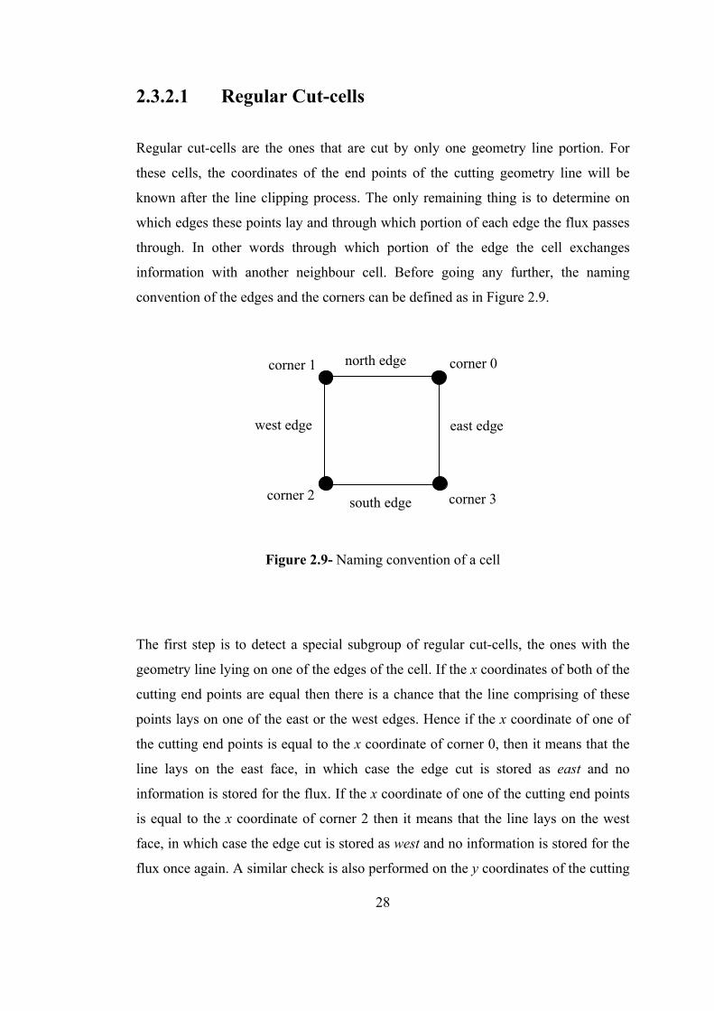
2.3.2.1 Regular Cut-cells
Regular cut-cells are the ones that are cut by only one geometry line portion. For
these cells, the coordinates of the end points of the cutting geometry line will be
known after the line clipping process. The only remaining thing is to determine on
which edges these points lay and through which portion of each edge the flux passes
through. In other words through which portion of the edge the cell exchanges
information with another neighbour cell. Before going any further, the naming
convention of the edges and the corners can be defined as in Figure 2.9.
Figure 2.9- Naming convention of a cell
The first step is to detect a special subgroup of regular cut-cells, the ones with the
geometry line lying on one of the edges of the cell. If the x coordinates of both of the
cutting end points are equal then there is a chance that the line comprising of these
points lays on one of the east or the west edges. Hence if the x coordinate of one of
the cutting end points is equal to the x coordinate of corner 0, then it means that the
line lays on the east face, in which case the edge cut is stored as east and no
information is stored for the flux. If the x coordinate of one of the cutting end points
is equal to the x coordinate of corner 2 then it means that the line lays on the west
face, in which case the edge cut is stored as west and no information is stored for the
flux once again. A similar check is also performed on the y coordinates of the cutting
east edge
north edge
west edge
south edge
corner 0corner 1
corner 2 corner 3

29
edge; if they are equal to each other and to one of the y coordinates of corner 0 or
corner 2, then the edge cut is stored as north or south respectively and no flux
information is stored. Thus for the special subgroup of regular cut-cells only one
edge is marked as cut while no information on the flux is stored.
Once the subgroup of special cells is detected the information for the other regular
cut-cells can be determined by edge based tests. Starting from the east edge and
going counter-clockwise, it is checked whether any of the edges is cut by one of the
end points of the geometry line or not. For the east face, it is checked whether the x
coordinates of the end points of the line are equal to the x coordinate of corner 0. If
one of them is equal then the east edge is marked as being cut, making corner 0,
corner 3 and any point in between along the east edge a candidate for the location of
the cutting end point. To determine the flux information, a point along the east edge
whose location relative to the cutting end point is known must be tested to see if it is
inside the body or outside it. The inside-outside test employed is based on the simple
point location test described in (15). The two possible points are corner 0 and corner
3. If the cutting end point is not on corner 0 this point is tested. If it is outside, the
flux for the east edge is marked as larger indicating that the flux passes through the
portion of the east edge with y coordinates greater than the one of the cutting end
point. Otherwise smaller is stored for the east face flux indicating that the flux passes
through the portion of the east edge with y coordinates less than the one of the
cutting end point. If the cutting end point is on corner 0 then corner 3 is tested and if
it is outside smaller is stored if it is inside larger is stored. If the east edge is not cut
then the centre of the edge is put to the inside-outside test, and if this point is outside
any of the bodies then the flux information is stored as all, indicating that the flux
passes through the whole face and otherwise it is stored as none, indicating that no
flux passes through the face.
Once the configuration of the east face is determined it is checked whether any of the
cutting end points lay on the north face. If a point is detected to be on the north face
the possible locations for it are either corner 1 or anywhere along the north edge
between corner 0 and corner 1. For the inside-outside test corner 0 is used since it is
already known that the cutting edge cannot be on this point. If corner 0 is outside,

30
then the flux is stored as larger, meaning that it passes through the portion of the
edge with x coordinates greater than the cutting edge otherwise smaller is stored
indicating that flux passes through the portion with x coordinates less than that of the
cutting edge. If the north edge is not cut then the centre of the edge is tested to see if
the flux passes through the whole face or it doesn’t pass at all.
After the north face the west face is examined. If this edge is cut, corner 1 is sent to
the inside-outside test as the only point along west edge on which the cutting end
point may not lay. The flux information is stored as larger if this point is outside
otherwise it is stored as smaller. If the edge is not cut, the centre of the edge is tested
to see if the flux passes through the face.
Finally, if the south face is cut either one of the corner 2 and corner 3 can be tested to
fill the flux information accordingly. If the edge is not cut, the centre of the edge is
tested to see if the flux passes through the face. In Figure 2.10, exemplifying cases
for regular cut-cells are illustrated.
Figure 2.10- Examples of regular cut-cells
In Figure 2.10, the scribbled parts represent the portion of the cell that is occupied by
a body. Case 1 is an example of the special subgroup of regular cells. In this
particular example the only cut edge is stored as the south edge and no flux
information is stored. In Case 2 the cut edges are detected as the east and west edges.
For the east face, the flux information is stored as larger even though no flux passes
through the face. The north flux information is all while for the west face it is larger
Case 1 Case 2 Case 3

31
and for the south face it is none. In Case 3, the edges cut are the north and west
edges. The flux information for the east and the south faces are all, it is larger for the
north face and smaller for the west face.
2.3.2.2 Irregular Cut-cells
The cut-cells that are cut by more than one geometry line are termed as irregular cut-
cells. To convert these cells into regular cut-cells, refinement is the first measure
taken. The cells that are cut by more than two geometry lines and those that are cut
by two lines that do not have a common end point are refined until their children are
cells of acceptable types or until they are refined to the maximum allowable level in
the mesh. It can safely be said that there will be no cells cut by more than two
geometry lines as a result of this refinement process, since the maximum level a cell
can reach will make it much smaller than the dimensions of the body. The cells that
are cut by two lines that do not have a common end point will eventually become
regular cut-cells if they are refined unconditionally. But sometimes they will require
very extensive refinement reaching levels much higher than the maximum allowable
one especially in the presence of very acute angles. These cases along with the cells
that are cut by two lines that have a common end point are treated separately.
In contrast to the other types, cells that are cut by two lines that have a common end
point are not refined unconditionally until they reach the maximum allowable level.
Instead they are refined, only when their distinct end points lay on the same face of
the cell as in Case 2 and Case 5 of Figure 2.11. The reason for this is that since the
bodies are represented as lines with specified end points, there would be a clustering
of highly refined cells around each of the specified points if these cells were to be
refined unconditionally. Those cells that are refined, the ones that have their distinct
end points on the same edges, are tested to see if they are concave or convex. If they
are convex, then they are simply converted to inside cells as in Case 2 of Figure 2.11.
At the end of this refinement process, the cells that were not converted are classified
into two groups; convex-united and concave-split and treated accordingly. The first

32
group is formed of cells that are cut by two lines without a common end point with a
single convex area (Case 3 of Figure 2.11), and the cells that are cut by two lines
with a common end point with the distinct end points on separate edges forming a
single convex cell area (Case 4 of Figure 2.11). The second group of cells are the
ones that are cut by two lines without a common end point with two separate convex
cell areas (Case 5 of Figure 2.11), cells that are cut by two lines with a common end
point forming a single concave area (Case 6 of Figure 2.11). The grouping and the
treatment of the irregular cut-cells can be depicted as in Figure 2.11.
Figure 2.11- Grouping and treatment of irregular cut-cells
2.3.2.2.1 Concave-Split
The concave-split cells are converted to regular cut-cells by making modifications on
the body. The location of the end points on the edges and the direction towards
which the lines converge is of essential importance in the conversion process. The
basic idea is to trim the body towards the direction in which the cutting lines
Case 1- Refine unconditionally till converted
Case 2- Refine till maxlevel then convert to inside
Case 3- Refine till maxlevel then treat as convex-united
Case 4- Treat as convex-united without refinement
Case 5- Refine till maxlevel then treat as concave-split
Case 6- Treat as convex-united without refinement

33
converge. Hence the geometry line cutting the cell will be the connection of the end
points in the diverging direction. The direction towards which the lines converge can
be determined by placing one coordinate of the end points of a line to the equation of
the other line to obtain the corresponding other coordinate. Then the line converges
towards the direction in which the difference between the calculated coordinate and
the coordinate of the end point is smaller. This can be represented more clearly
graphically as in Figure 2.12.
Figure 2.12- Conversion of an irregular cut-cell
The criterion for the above conversion is expressed mathematically in the following
equation.
2 0 2 10 3 2 2 1 3 2 2
2 3 2 3
( - ) ( - )- ( - ) - ( - )( - ) ( - )
x x x xy y y y y y y yx x x x
⎡ ⎤ ⎡ ⎤+ > +⎢ ⎥ ⎢ ⎥
⎣ ⎦ ⎣ ⎦ (2.20)
This trimming process will result in obtaining a member of the special subgroup of
regular cut-cells in some cases, while regular cut-cells are obtained in some cases.
The special subgroup will be obtained for cells that are cut by lines with a common
end point having their distinct end points on the same edge, cells having two pairs of
end points on the same edge and cells that have one pair of end points on the same
edge while converging towards the end points that are on different edges. These
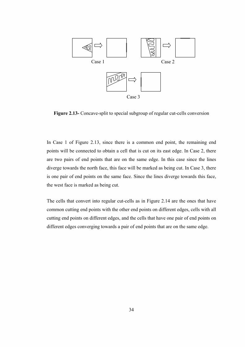
cases and their conversion are illustrated in Figure 2.13.
x0,y0
x1,y1 x2,y2
x3,y3
x0,y0
x2,y2
34
Figure 2.13- Concave-split to special subgroup of regular cut-cells conversion
In Case 1 of Figure 2.13, since there is a common end point, the remaining end
points will be connected to obtain a cell that is cut on its east edge. In Case 2, there
are two pairs of end points that are on the same edge. In this case since the lines
diverge towards the north face, this face will be marked as being cut. In Case 3, there
is one pair of end points on the same face. Since the lines diverge towards this face,
the west face is marked as being cut.
The cells that convert into regular cut-cells as in Figure 2.14 are the ones that have
common cutting end points with the other end points on different edges, cells with all
cutting end points on different edges, and the cells that have one pair of end points on
different edges converging towards a pair of end points that are on the same edge.
Case 1 Case 2
Case 3

35
Figure 2.14- Concave-split to regular cut-cells conversion
In Case 1 of Figure 2.14, there is a common end point and the other end points are
connected automatically to form a regular cut-cell. In Case 2, all the end points are
on distinct edges. Since the distance between the ones on the west and the south
edges is greater than the distance between the others the cut locations on these edges
are connected to form a regular cut-cell. In Case 3, since the lines diverge towards
the end points that are on different edges in contrast to Case 3 of Figure 2.13, a
regular cut-cell is formed by the connection of the cut location on these edges.
2.3.2.2.2 Convex-United
The procedure followed for the convex-united cells are similar to the ones for
concave-split cells. Once again the end points towards which the cutting lines
diverge are connected to form the new cutting edge. In the case of the convex-united
cells conversion is made to either an inside cell or to a regular cut-cell. The cells that
have two pairs of cutting end points on the same faces, and the cells that have a pair
of end points on the same edge with the lines converging towards the end points that
are on different edges are converted to inside cells. These cases are illustrated in
Figure 2.15.
Case 1 Case 2
Case 3

36
Figure 2.15- Convex-united to inside cells conversion
Case 1 and Case 2 of Figure 2.15 are analogous to those presented in Figure 2.13.
With the difference that they convert to inside cells, and there is no special sub-group
of inside cells.
The cells that are converted to regular cut-cells are the ones that have common
cutting end points with the other end points on different edges, cells with all cutting
end points on different edges, and the cells that have one pair of end points on
different edges converging towards a pair of end points that are on the same edge.
These cases are illustrated in Figure 2.16.
Figure 2.16- Convex-united to regular cut-cells conversion
Case 1 Case 2
Case 3
Case 1 Case 2

37
The Case 1, Case 2 and Case 3 of Figure 2.16 are analogous to those in Figure 2.14.
The difference between them is the portions of the cells that are marked as inside and
outside are opposite in these cases.
Since each irregular cell is converted individually into a cut-cell, at the end of the
process some cut-cells that are not part of any body will be obtained. Hence, at the
end of the conversion process, the mesh has to be traversed to find these unconnected
cells and convert them into either outside cells, if they were processed as concave-
split cells, or into inside cells if they were treated as convex-united cells.
2.3.3 Curvature Adaptation
The last step in the mesh generation process is the curvature adaptation. The purpose
of the curvature adaptation is to ensure that regions of a body that have high
curvatures are resolved enough to be represented accurately and also since these
regions will be associated with high gradients.
In curvature adaptation, the cutting edges of neighbouring cut-cells are evaluated to
decide on whether to refine a cell or not. So firstly neighbouring cut-cells should be
detected then curvature must be quantified to develop a criterion for refinement. In
order to quantify the curvature, the angle between the normals of the cutting edges
pointing towards the fluid domain is used. If this quantity exceeds a threshold value
then the cell is refined. This can be illustrated as in Figure 2.17.

38
Figure 2.17- The normals of two neighbouring cut-cells
The normal for a cutting edge of a cell can be determined through the flux
information stored for a cut edge.
Figure 2.18- Calculation of the normal
In Case 1 of Figure 2.18, the first edge that is cut is the east edge and the flux
information associated is larger. In this case, the normal is given by the following
equation.
0 1 0 1- -( - ) ( - )n yi xj y y i x x j= ∆ + ∆ = + (2.21)
∆x∆y
∆x∆y
x0,y0
x1,y1
x0,y0
x1,y1
n
n
Case 1 Case 2
θ: The angle between normals

39
In Case 2, the first edge cut is east as in the previous case but this time the associated
flux information is smaller making the normal;
0 1 0 1- ( - ) - ( - )n yi xj y y i x x j= ∆ ∆ = (2.22)
Hence, it is possible to express each normal pointing to the fluid domain using the
first edge cut and the flux information associated with it for the neighbouring cells.
Then, a relation for the angle between the normals can be obtained by their dot
multiplication as
1 2 1 21 2 1 2 1 2 1 2
1 2
( )| || | cos cos
| || |x x y y
x x y y
n n n nn n n n n n n n
n nθ θ
+= + = ⇒ =i (2.23)
Then a cell is to be refined, if this θ value is greater than a threshold value.
1 2 1 2
1 2
( )cos cos
| || |x x y y
th
n n n nn n
θ θ+
= < (2.24)

40
CHAPTER 3
NUMERICAL METHOD
3.1 Governing Equations
In the code developed, solution to the compressible Euler equations in the conserved
form is sought. Hence, the governing equations can be represented as
0dV ndAt∂
+ =∂ ∫∫∫ ∫∫U Fi (3.1)
where, U and F are the vectors of conserved variables and the flux respectively,
while n is the normal to the differential area element dA . This equation can be
descritised in 2-D as
1 0edgescell
n st A
∂+ ∆ =
∂ ∑U Fi (3.2)
n being the face normal, s∆ the edge length and cellA the cell area. The vector of
conserved variables and the flux vector can be written as
2
2
cos sincos sin cos
sin cos sin
cos sint t t
u vu u uv p
nv v uv pe uh vh
ρ ρ θ ρ θρ ρ θ ρ θ θρ ρ θ ρ θ θρ ρ θ ρ θ
+⎡ ⎤ ⎡ ⎤⎢ ⎥ ⎢ ⎥+ +⎢ ⎥ ⎢ ⎥= =⎢ ⎥ ⎢ ⎥+ +⎢ ⎥ ⎢ ⎥+⎢ ⎥ ⎢ ⎥⎣ ⎦ ⎣ ⎦
U Fi (3.3)
In this equation θ is the angle between the normal direction of the edge and the
Cartesian x-direction. The variables , , , , tu v p eρ and th are the density, velocity in

41
the x and y direction, the pressure, the total energy and the total enthalpy
respectively.
In the solution method used, determination of the fluxes through the faces of the cells
require a pseudo one dimensional form of the flux vector represented in Equation
(3.3). This form will be equivalent to the Euler equations written in terms of the
normal and tangential velocities. At this point, the rotational invariance of the Euler
equations (16) can be employed as
1 1 ˆ ˆ( ) ( )n − −= =F T F TU T F Ui (3.4)
The transformation matrix and its inverse; T and -1T , appearing in Equation (3.4)
can be written explicitly as
1
1 0 0 0 1 0 0 00 cos sin 0 0 cos sin 0
0 sin cos 0 0 sin cos 00 0 0 1 0 0 0 1
θ θ θ θθ θ θ θ
−
⎡ ⎤ ⎡ ⎤⎢ ⎥ ⎢ ⎥−⎢ ⎥ ⎢ ⎥= =⎢ ⎥ ⎢ ⎥−⎢ ⎥ ⎢ ⎥⎣ ⎦ ⎣ ⎦
T T (3.5)
Hence, the conserved quantities and the flux vector in terms of normal and
tangential velocities can be given
2
ˆˆ ˆˆ ˆ ˆ ( )ˆ ˆ ˆ
ˆt t
uu u pv uve uh
ρ ρρ ρρ ρρ ρ
⎡ ⎤ ⎡ ⎤⎢ ⎥ ⎢ ⎥+⎢ ⎥ ⎢ ⎥= =⎢ ⎥ ⎢ ⎥⎢ ⎥ ⎢ ⎥⎢ ⎥ ⎢ ⎥⎣ ⎦ ⎣ ⎦
U F U (3.6)
In Equation (3.6) u and v are the normal and tangential velocities, while U and F are
the vectors of conserved variables and the flux, in terms of the normal and tangential
velocities. The normal and the tangential velocities can be expressed in terms of the
Cartesian velocities as
ˆ ˆcos sin , sin cosu u v v u vθ θ θ θ= + = − + (3.7)

42
Using this transformation, the governing equations can be expressed as
11 ˆ ˆ 0edgescell
st A
−∂+ ∆ =
∂ ∑U T F(U) (3.8)
The general solution strategy is to estimate the flux in terms of the normal and
tangential directions, rotate them to Cartesian coordinates with the inverse
transformation matrix for each face, and then use an appropriate method for time
integration.
3.2 One Dimensional Riemann Problem for Linear Systems
Before discussing the solution algorithm for the Euler equations, the one dimensional
Riemann problem for a linear system of equations should be discussed (17) (16). The
model equation for the one dimensional linear system is represented by Equation
(3.9). This equation is linear if the Jacobian of the flux vector is comprised of
constant elements, that is
0t x t x t x
∂ ∂ ∂ ∂ ∂ ∂ ∂+ = + = + =
∂ ∂ ∂ ∂ ∂ ∂ ∂U F U F U U UA
U (3.9)
where A is the Jacobian matrix. The initial conditions for the model equation are
given as
0
0
0( ,0)
0x
xx<⎧
= ⎨ >⎩L
R
UU
U (3.10)
where subscripts L and R refer to the left and right states respectively. The first step
in the solution process is to diagonalize the Jacobian matrix using the Q matrix
appearing in the following equation. Each column of this matrix is a right
eigenvector of the Jacobian matrix and the rows of its inverse are the left
eigenvectors of the Jacobian matrix (18). The elements of the resulting diagonal
matrix Λ are the eigenvalues of the Jacobian matrix.

43
−1Q AQ = Λ (3.11)
Using this diagonalization and multiplying Equation (3.9) by Q-1, the linear set of
equations can be converted to a set of independent equations in terms of the new
characteristic variable vector V .
0t x t x
∂ ∂ ∂ ∂+ = + =
∂ ∂ ∂ ∂-1 -1 -1U U V VQ Q AQQ Λ (3.12)
The relation between the characteristic variables and the conserved quantities in
Equation (3.12) can be defined as
∂ = ∂-1Q U V (3.13)
Since this is a linear system and the elements of Q-1 are constant, Equation (3.13) can
be written in an alternative form as
= ⇒ ∆ = ∆-1 -1Q U V Q U V (3.14)
where;
∆ = − ∆ = −R L R LV V V U U U
After the diagonalization, the governing equations obtained in terms of the
characteristic variables,λ ’s, in Equation (3.12) can be written explicitly as
1 1 10 . . 0. 0 . . .. . . . . 0. . . 0 .
0 . . 0n n nt x
v v
v v
λ
λ
⎡ ⎤ ⎡ ⎤ ⎡ ⎤⎢ ⎥ ⎢ ⎥ ⎢ ⎥⎢ ⎥ ⎢ ⎥ ⎢ ⎥⎢ ⎥ ⎢ ⎥ ⎢ ⎥+ =⎢ ⎥ ⎢ ⎥ ⎢ ⎥⎢ ⎥ ⎢ ⎥ ⎢ ⎥⎢ ⎥ ⎢ ⎥ ⎢ ⎥⎣ ⎦ ⎣ ⎦ ⎣ ⎦
(3.15)

44
The equations represented by Equation (3.15) are n independent equations for the n
characteristic variables. In other words, n independent scalar equations are obtained
for n characteristic variables, 'sv , (17) as
1,...,i ii
v v i nt x
λ∂ ∂+ =
∂ ∂ (3.16)
For the solution of each one of the equations in Equation (3.16), the definition of the
total derivative is employed as
d dd d
i i iv v v xt t x t
∂ ∂= +∂ ∂
(3.17)
Hence with the application of the condition presented in Equation (3.18), a straight
line along which the characteristic variable remains constant and the governing
equation is satisfied, is obtained.
0dd 0 along line
d di
i ivx x x t
t tλ λ= ⇒ = = + (3.18)
The solution obtained in terms of the characteristic lines can be represented
graphically as in Figure 3.1.
Figure 3.1- Solution of a 1-D Riemann problem for a set of linear equations
x=λ1t x=λnt

45
In Figure 3.1, when one of the characteristic lines is crossed the respective value of
the characteristic variable changes conforming to the given initial conditions. The
form in which the solution is presented is of crucial importance in the development
of numerical methods while it doesn’t make a difference in the analytical sense.
Hence the solution can be presented in several formats (17). First representation is in
terms of the characteristic variables as
1
2 1 2
1
... / ...... / ...
. .
. .
. .... ... /
n
n
n
x tx t
xt
x t
λ λλ λ λ
λ λ
= −∆ − −∆ < < <⎧⎪ + ∆ = −∆ − −∆ < < < <⎪⎪⎪⎛ ⎞ = ⎨⎜ ⎟
⎝ ⎠ ⎪⎪⎪
+ ∆ + + ∆ = < < <⎪⎩
L R 1 n
L 1 R n
L 1 n R
V V v vV v V v v
V
V v v V
(3.19)
The difference vectors appearing in Equation (3.19) can be written explicitly as
1
1
00.0 ... .
... ..0. .
0 0
ni
n
v
v vv
v
∆ ⎡ ⎤⎡ ⎤ ⎡ ⎤⎢ ⎥⎢ ⎥ ⎢ ⎥⎢ ⎥⎢ ⎥ ⎢ ⎥⎢ ⎥⎢ ⎥ ⎢ ⎥
∆ = ∆ = ∆ = ⇒ ∆ + + ∆ = ∆⎢ ⎥⎢ ⎥ ⎢ ⎥∆ ⎢ ⎥⎢ ⎥ ⎢ ⎥⎢ ⎥⎢ ⎥ ⎢ ⎥⎢ ⎥⎢ ⎥ ⎢ ⎥∆⎢ ⎥ ⎢ ⎥ ⎢ ⎥⎣ ⎦ ⎣ ⎦ ⎣ ⎦
1 i nv v v V (3.20)
It is possible to express the solution in terms of the conserved variables as well by
employing the relation between the characteristic variables and the conserved
variables given in Equation (3.14). Here it should be remembered that each column
of matrix Q is an eigenvector of the Jacobian matrix. This will promote the relation
presented in the following equation
iv∆ = ∆i iQ v r (3.21)
where ri is the ith eigenvector of the Jacobian matrix.

46
Hence by multiplying Equation (3.19) by the matrix Q, the solution in terms of the
conserved variables is obtained as
1 1
1 2 2 1 2
1 1
... / ...... / ...
. .
. .
. .... ... /
n n
n n
n n
v v x tv v v x t
xt
v v x t
λ λλ λ λ
λ λ
= − ∆ − − ∆ < < <⎧⎪ + ∆ = − ∆ − − ∆ < < < <⎪⎪⎪⎛ ⎞ = ⎨⎜ ⎟
⎝ ⎠ ⎪⎪⎪
+ ∆ + + ∆ = < < <⎪⎩
L R 1 n
L 1 R n
L 1 n R
U U r rU r U r r
U
U r r U
(3.22)
At this point, it should be noted that for the numerical method that is used for the
solution of the Euler equations, the flux at a face of a certain cell will be of interest
rather than the value of the conserved variable. It should also be noted that the flux
vector appearing in the differential model equation is equivalent to the flux term that
would appear in its integral formulation. Also the fluxes of each face will be
investigated separately so the / can be considered to be zero for the respective face
of the cell. Taking these points into consideration one can derive expressions for the
fluxes as a solution.
( )
1 1 1
1 1 2 2 2 1 2
1 1 1
... 0 ...... 0 ...
. .0
. .
. .... ... 0
n n n
n n n
n n n
v vv v v
v v
λ λ λ λλ λ λ λ λ λ
λ λ λ λ
= − ∆ − − ∆ < < <⎧⎪ + ∆ = − ∆ − − ∆ < < < <⎪⎪⎪= ⎨⎪⎪⎪
+ ∆ + + ∆ = < < <⎪⎩
L R 1 n
L 1 R n
L 1 n R
AU AU r rAU r AU r r
F
AU r r AU
(3.23)
Equation (3.23) has been obtained by exploiting the fact that iλ=i iAr r .
Even though Equation (3.23) is a perfectly valid representation of the solution, it is
desirable to present the solution in a more compact form as in one of the following
equivalent forms:

47
1
1
(0)
(0)
n
i ii
n
i ii
v
v
λ
λ
−
=
+
=
= + ∆
= − ∆
∑
∑
L i
R i
F AU r
F AU r (3.24)
where;
min(0, )
max(0, )i i
i i
λ λ
λ λ
−
+
=
=
Since the representation is dependent on the sign of the eigenvalues in Equation
(3.24), a final form for the solution can be obtained by averaging the equivalent
solutions appearing in Equation (3.24).
[ ]
11 ( ) ( )2
1 1(0) ( )2 2
n
i ii
vλ=
+
= + − ∆∑L R
L R i
F U F U
F A U U r (3.25)
3.3 The Approximate Riemann Solver of Roe
The flux term in the governing Euler equations in the integral form (3.1) can be
estimated by considering the x-split form of the two dimensional Euler equations in
the differential form as
0t x y
∂ ∂ ∂+ + =
∂ ∂ ∂U F G (3.26)
where;
1 1 12
2 2 22
3 3 3
4 4 4
t t t
u vu f gu u p uvu f gv uv v pu f ge uh vhu f g
ρ ρ ρρ ρ ρρ ρ ρρ ρ ρ
⎡ ⎤ ⎡ ⎤ ⎡ ⎤⎡ ⎤ ⎡ ⎤ ⎡ ⎤⎢ ⎥ ⎢ ⎥ ⎢ ⎥⎢ ⎥ ⎢ ⎥ ⎢ ⎥+⎢ ⎥ ⎢ ⎥ ⎢ ⎥⎢ ⎥ ⎢ ⎥ ⎢ ⎥= = = = = =⎢ ⎥ ⎢ ⎥ ⎢ ⎥⎢ ⎥ ⎢ ⎥ ⎢ ⎥ +⎢ ⎥ ⎢ ⎥ ⎢ ⎥⎢ ⎥ ⎢ ⎥ ⎢ ⎥
⎢ ⎥ ⎢ ⎥ ⎢ ⎥⎢ ⎥ ⎢ ⎥ ⎢ ⎥⎣ ⎦ ⎣ ⎦ ⎣ ⎦⎣ ⎦ ⎣ ⎦ ⎣ ⎦
U F G

48
As can be observed the flux vector in Equation (3.26) is identical to the one
appearing in the transformed form of the governing equations given by Equation
(3.6). The theory of the Riemann problem for one dimensional linear systems will be
employed to estimate this flux.
To obtain the Jacobian for the x-split Euler equations, the flux vector must be written
in terms of the conserved variables as
( )
( )
2
22 232 2
41 1 1
2 3
1
233 22 4 2 4 2
2 21 1 1 1
12 2
12 2
u
uu uuu u u
u uu
u uu u u u uu u u u
γ
γ
⎡ ⎤⎢ ⎥
⎛ ⎞⎢ ⎥+ − − −⎜ ⎟⎢ ⎥⎝ ⎠⎢ ⎥= ⎢ ⎥⎢ ⎥⎢ ⎥⎢ ⎥⎛ ⎞
+ − − −⎢ ⎥⎜ ⎟⎢ ⎥⎝ ⎠⎣ ⎦
F (3.27)
In Equation (3.27) γ is the specific heat ratio. Noting that the Jacobian matrix is
specified in the following form
1 1 1 2 1 3 1 4
2 1 2 2 2 3 2 4
3 1 3 2 3 3 3 4
4 1 4 2 4 3 4 4
/ / / // / / // / / // / / /
f u f u f u f uf u f u f u f uf u f u f u f uf u f u f u f u
∂ ∂ ∂ ∂ ∂ ∂ ∂ ∂⎡ ⎤⎢ ⎥∂ ∂ ∂ ∂ ∂ ∂ ∂ ∂∂ ⎢ ⎥= =⎢ ⎥∂ ∂ ∂ ∂ ∂ ∂ ∂ ∂∂⎢ ⎥∂ ∂ ∂ ∂ ∂ ∂ ∂ ∂⎢ ⎥⎣ ⎦
F AU
(3.28)
it can be obtained by equations (3.27) and (3.28) in terms of the flow variables.
( ) ( ) ( )
( ) ( ) ( )
2 2
2 2
0 1 0 01 3 1 1
0
2 1 1
t
t t
h u a u vuv v u
u h a h u uv u
γ γ γ γ
γ γ γ γ
⎡ ⎤⎢ ⎥− − − − − −⎢ ⎥= ⎢ ⎥−⎢ ⎥
⎡ ⎤− − − − − −⎢ ⎥⎣ ⎦⎣ ⎦
A (3.29)
In Equation (3.29) a is the speed of sound. As can be observed from Equation (3.29),
the Jacobian matrix does not have constant elements hence the Euler equations are

49
not linear. For the approximate Riemann solvers this Jacobian matrix is replaced by
one that has constant elements since for a non-linear system the characteristic lines of
the same family will not be parallel introducing shock waves and expansion fans into
the solution (17), (16).
In Roe’s approximate Riemann solver (19), the Jacobian matrix is expressed in terms
of an intermediate state defined from the right and left states.
First, it is observed that both the flux vector F and the vector of conserved quantities
U are quadratic in terms of a new vector W defined as
1
2
3
4
1
t
wuwvwhw
ρ
⎡ ⎤⎡ ⎤⎢ ⎥⎢ ⎥⎢ ⎥⎢ ⎥= =⎢ ⎥⎢ ⎥⎢ ⎥⎢ ⎥
⎢ ⎥ ⎢ ⎥⎣ ⎦ ⎣ ⎦
W (3.30)
Another useful vector, W , is formed by taking the arithmetic mean of the W vector
for the right and left states.
1
2
3
4
2
2
2
2
L R
L L R R
L L R R
L tL R tR
w u uww v vw
h h
ρ ρ
ρ ρ
ρ ρ
ρ ρ
⎡ ⎤+⎢ ⎥⎢ ⎥⎢ ⎥⎡ ⎤ +⎢ ⎥⎢ ⎥⎢ ⎥⎢ ⎥= =⎢ ⎥⎢ ⎥ +⎢ ⎥⎢ ⎥
⎢ ⎥⎣ ⎦ ⎢ ⎥⎢ ⎥+⎢ ⎥⎢ ⎥⎣ ⎦
W (3.31)
It is now possible to express the difference between the right and the left states for
the conserved quantities in terms of the new vector defined as
∆ = ∆U B W (3.32)
where;

50
1
2 1
3 1
4 12 3
2 0 0 00 0
0 01 1
ww ww ww ww wγ γγ γ γ γ
⎡ ⎤⎢ ⎥⎢ ⎥
= ⎢ ⎥⎢ ⎥− −⎢ ⎥⎢ ⎥⎣ ⎦
B
It is also possible to express the differential flux vector in terms of the vector W in
the same manner as
∆ = ∆F C W (3.33)
where;
2 1
4 2 3 1
3 2
4 2
0 01 1 1 1
0 00 0
w w
w w w w
w ww w
γ γ γ γγ γ γ γ
⎡ ⎤⎢ ⎥− + − −⎢ ⎥−
= ⎢ ⎥⎢ ⎥⎢ ⎥⎢ ⎥⎣ ⎦
C
Using Equations (3.32) and (3.33) it is possible to establish a direct relation between
the difference in the flux vector and the vector of conserved quantities in the form
∆ = ∆-1CB U F (3.34)
Using the homogeneity property of the Euler equations given by the following
equation (16) one can recognize the product CB-1 as the Jacobian matrix.
∂=∂
A
FF UU
(3.35)
In order to find the eigenvalues of the Jacobian matrix, the following equation must
be solved.

51
( ) ( )det 0 det 0λ λ− = ⇒ − =-1CB I C B (3.36)
Dividing Equation (3.36) by 1w , it is possible to find the eigenvalues of the Jacobian
in terms of the new variables defined as
2
1
L L R R
L R
u uwuw
ρ ρρ ρ
+= =
+ (3.37)
3
1
L L R R
L R
v vwvw
ρ ρρ ρ
+= =
+ (3.38)
4
1
L tL R tRt
L R
h hwhw
ρ ρρ ρ
+= =
+ (3.39)
( ) ( )2 21 11 12 2t ta h V e Vγ γ γ⎛ ⎞ ⎛ ⎞= − − = − −⎜ ⎟ ⎜ ⎟
⎝ ⎠ ⎝ ⎠ (3.40)
L Rρ ρ ρ= (3.41)
1 2 3 4 u a u u aλ λ λ λ= − = = = + (3.42)
The corresponding right eigenvectors can also be expressed in terms of the new Roe
averaged quantities as
2 3 4
2
11 100
1
12t t
uu a u avv v
vVh ua h ua
⎡ ⎤⎡ ⎤ ⎡ ⎤⎡ ⎤⎢ ⎥⎢ ⎥ ⎢ ⎥⎢ ⎥− +⎢ ⎥⎢ ⎥ ⎢ ⎥⎢ ⎥= = = =⎢ ⎥⎢ ⎥ ⎢ ⎥⎢ ⎥⎢ ⎥⎢ ⎥ ⎢ ⎥⎢ ⎥⎢ ⎥− +⎢ ⎥ ⎢ ⎥⎣ ⎦⎣ ⎦ ⎣ ⎦⎢ ⎥⎣ ⎦
1r r r r (3.43)

52
With the right eigenvectors defined as in Equation (3.43), it is possible to determine
the characteristic variables which can also be termed as the wave strengths by using
Equation (3.14).
1 1
2 2
3 32
4 4
11 1001
12t t
v uuu a u a v uvv v v u
v uvVh ua h ua
⎡ ⎤ ∆ ∆⎡ ⎤ ⎡ ⎤⎢ ⎥ ⎢ ⎥ ⎢ ⎥− +⎢ ⎥ ∆ ∆⎢ ⎥ ⎢ ⎥=⎢ ⎥ ⎢ ⎥ ⎢ ⎥∆ ∆⎢ ⎥ ⎢ ⎥ ⎢ ⎥⎢ ⎥ ∆ ∆− + ⎢ ⎥ ⎢ ⎥⎣ ⎦ ⎣ ⎦⎢ ⎥⎣ ⎦
(3.44)
Due to the proportionality between the coefficients of the first and third relations in
Equation (3.44), it is possible to eliminate the third equation by using the first one to
obtain the following relation.
3 3 1v u v u∆ = ∆ − ∆ (3.45)
Then a set of three equations is obtained for three wave strengths as
4 1
1 22
2 2 4 1 3
1 1 1
12t t
v uu a u a u v u
v u v u v uh ua h ua V
⎡ ⎤⎢ ⎥ ∆ ∆⎡ ⎤ ⎡ ⎤⎢ ⎥ ⎢ ⎥ ⎢ ⎥+ − ∆ = ∆⎢ ⎥ ⎢ ⎥ ⎢ ⎥⎢ ⎥ ⎢ ⎥ ⎢ ⎥∆ ∆ + ∆ − ∆⎣ ⎦ ⎣ ⎦+ −⎢ ⎥⎣ ⎦
(3.46)
It is possible to solve this system using Gauss elimination to obtain the wave
strengths as
( ) ( )22 1 2 4 3 12
1tv u h u u u u v u v u
aγ − ⎡ ⎤∆ = ∆ − + ∆ − ∆ + ∆ − ∆⎣ ⎦ (3.47)
( )1 1 2 21
2v u a u u a v
a∆ = + ∆ − ∆ − ∆⎡ ⎤⎣ ⎦ (3.48)
4 1 1 2( )v u v v∆ = ∆ − ∆ +∆ (3.49)

53
Defining an operator given by the following equation
( )2( )pq p q q p O∆ = ∆ + ∆ + ∆ (3.50)
neglecting higher order terms and placing the values of the conserved quantities, the
wave strengths can be expressed in terms of the flow variables as
( ) ( )
( )
2 22 2
2 2
1
1
t t t
t t t
v h u u u u e e v v v va
v h e u u v v ea
γ ρ ρ ρ ρ ρ ρ ρ ρ
γ ρ ρ ρ ρ
− ⎡ ⎤∆ = ∆ − + ∆ + ∆ − ∆ − ∆ + ∆ + ∆ − ∆⎣ ⎦
− ⎡ ⎤⇒ ∆ = ∆ − + ∆ + ∆ − ∆⎣ ⎦
(3.51)
The terms appearing in Equation (3.51) must be treated individually to simplify the
expression. For the treatment of the first term in the brackets, Equation (3.40) can be
employed as
( ) ( )2 2 2
2 21 11 2 1 2t t
a a ah e V Vρ ρ ργ γ γ γ
⎛ ⎞∆ − = ∆ + − − = ∆⎜ ⎟⎜ ⎟− −⎝ ⎠
(3.52)
The last term in the brackets must also be treated individually with the aid of the
relation
21
1 2tp Ve
γ ρ= +
− (3.53)
To obtain
( ) ( )2
2 21 11 2 1 1t
p p ae u v u u v vρρ ρ ρ ργ ρ γ γ γ⎡ ⎤⎛ ⎞ ∆ ∆
∆ = ∆ + ∆ + = − + ∆ + ∆⎢ ⎥⎜ ⎟− − −⎝ ⎠⎣ ⎦ (3.54)
Substituting Equations (3.52) and (3.54) into Equation (3.51), a simplified equation
for the wave strength can be obtained. Then applying the operator defined in

54
Equation (3.50) and substituting Equation (3.57) into Equations (3.48) and (3.49) all
the wave strengths can be found as
( )1 2
12
v p a ua
ρ∆ = ∆ − ∆ (3.55)
2 2
pva
ρ ∆∆ = ∆ − (3.56)
3v vρ∆ = ∆ (3.57)
( )4 2
12
v p a ua
ρ∆ = ∆ + ∆ (3.58)
In summary, for the approximate Riemann solver of Roe, first the Jacobian matrix
for the Euler equations, which are non linear in their true essence, have been replaced
by another matrix with constant elements to approximate the governing equations as
a linear system. Thereafter the eigenvalues and eigenvectors of this approximate
Jacobian matrix are found by following the procedure outlined in (19). Then these
are used to find the wave strengths, characteristic variables, and fluxes through a face
for which the right and left states are known according to Equation (3.25).
3.3.1 Solution Algorithm
The solution algorithm adopted is similar to the one outlined in (16). The algorithm
discussed here is for the determination of the flux through a certain face of the cell
under investigation. Once the fluxes through all the faces are determined, an
appropriate method for time integration, to be discussed later, is employed to update
the values of the conserved variables.
(i) First the conserved variables of the left and right states are obtained by
reconstruction which will be explained later on.

55
(ii) The primitive variables, [ ]Ttu v P hρ for the right and left states are
determined from the conserved variables [ ]Ttu v eρ ρ ρ ρ
simultaneously with the transformation to normal and tangential coordinates.
The flux which will be used in Equation (3.25), is calculated from the left and
right state variables.
cos sinˆ u vu ρ θ ρ θρ+
= (3.59)
sin cosˆ u vv ρ θ ρ θρ
− += (3.60)
( )2 2( ) ( )1 t
u vp e ρ ργ ρρ ρ
⎡ ⎤= − − −⎢ ⎥
⎣ ⎦ (3.61)
( )1t th e pρ
ρ= + (3.62)
(iii) The Roe averaged quantities for the transformed primitive variables and the
eigenvalues are calculated from Equations (3.37) through (3.42).
(iv) The wave strengths are calculated from Equations (3.55) through (3.58). The
differences are taken as the right minus the left state variables in contrast to
Roe’s derivation in (19) to be consistent with Equation (3.25).
(v) The right eigenvectors are calculated using the transformed Roe averaged
quantities with the formulation provided in Equation (3.43).
(vi) The flux is calculated from Equation (3.25).
(vii) The flux obtained, which is normal to the face, is transformed back to the
Cartesian coordinates using the inverse transformation matrix.
ˆ =-1T F F (3.63)
where T-1 is given in Equation (3.5).

56
3.4 Flux Vector Splitting
In addition to using Roe’s approximate Riemann solver to evaluate the flux term
appearing in Equation (3.8), the flux vector splitting methods such as van Leer (20),
AUSM (21) and its derivatives AUSMD, AUSMV (22) have also been employed.
Considering Equation (3.9) it is possible to split the flux vector as
( ) ( ) ( )= ++ -F U F U F U (3.64)
The negative and positive components of the flux vector, +F and -F , can be defined
by splitting the Jacobian matrix as follows
( ) , ( )− −= =+ +F U A U F U A U (3.65)
, − −= =+ + -1 -1A QΛ Q A QΛ Q (3.66)
The diagonal matrices +Λ and −Λ can be defined as
1 10 . . 0 0 . . 00 . . 0 . .
, . . . . . .. . 0 . . 00 . . 0 0 . . 0m m
λ λ
λ λ
+ −
−
+ −
⎡ ⎤ ⎡ ⎤⎢ ⎥ ⎢ ⎥⎢ ⎥ ⎢ ⎥⎢ ⎥ ⎢ ⎥= =⎢ ⎥ ⎢ ⎥⎢ ⎥ ⎢ ⎥⎢ ⎥ ⎢ ⎥⎣ ⎦ ⎣ ⎦
+Λ Λ (3.67)
where the positive and negative eigenvalues can be defined as in (23) presented as in
the following equation.
( ) ( )1 1 , 2 2
λ λ λ λ λ λ+ −= + = − (3.68)
When the Euler equations are written in normal and tangential coordinates as in
Equation (3.8) the positive flux component will be due to the cell itself while the

57
negative component will be calculated from the neighbour as illustrated in Figure
3.2.
Figure 3.2- Graphical interpretation of flux vector splitting
In Figure 3.2 the left state is the cell under investigation while the right state is the
neighbour. The positive eigenvalues of the left state affects the face hence the
positive component of the flux is calculated from the left state while the negative
component of the flux is calculated from the right state since the negative
eigenvalues of this state affects the face. Further details can be found in (16).
3.4.1 Van Leer Flux Vector Splitting
The van Leer flux vector splitting algorithm (20) makes use of the flux represented in
terms of the density, tangential velocity, Mach number, M , and the speed of sound
as
( )
2 2
22 2 2
ˆ
1ˆˆˆ ˆ ˆ( ) ,
ˆ ˆ
1ˆ ˆ ˆ2 1
aM
a MuMaaMv
aaM a M v
ρ
ργ
ρ
ργ
⎡ ⎤⎢ ⎥
⎛ ⎞⎢ ⎥+⎜ ⎟⎢ ⎥⎝ ⎠⎢ ⎥= =⎢ ⎥⎢ ⎥
⎡ ⎤⎢ ⎥+ +⎢ ⎥⎢ ⎥−⎢ ⎥⎣ ⎦⎣ ⎦
F U (3.69)
Left Right
nt

58
The flux can then be split into its positive and negative components as presented in
the following equations.
( )2
222
2
12 1 ˆ 1
21ˆ ˆ1 ˆ4
2 1 1ˆ ˆ11 2 2
a Ma M
v
a M v
γγ
ρ
γγ
⎡ ⎤⎢ ⎥−⎛ ⎞⎢ ⎥+⎜ ⎟⎢ ⎥⎝ ⎠
= + ⎢ ⎥⎢ ⎥⎢ ⎥−⎛ ⎞⎢ ⎥+ +⎜ ⎟−⎢ ⎥⎝ ⎠⎣ ⎦
+F (3.70)
( )2
222
2
12 1 ˆ 1
21ˆ ˆ1 ˆ4
2 1 1ˆ ˆ11 2 2
a Ma M
v
a M v
γγ
ρ
γγ
−
⎡ ⎤⎢ ⎥−⎛ ⎞⎢ ⎥−⎜ ⎟⎢ ⎥⎝ ⎠
= − − ⎢ ⎥⎢ ⎥⎢ ⎥−⎛ ⎞⎢ ⎥− +⎜ ⎟−⎢ ⎥⎝ ⎠⎣ ⎦
F (3.71)
3.4.2 AUSM (Liou-Steffen) Flux Vector Splitting
The AUSM scheme (21) splits the pressure and the advection terms appearing in the
normal momentum flux as
( ) ( )1/ 2 1/ 2 1/ 21ˆ ˆ ˆ ˆ( )2 L R R LM M⎡ ⎤= + − − +⎣ ⎦F U φ φ φ φ p (3.72)
In equation (3.72), 1/2M is the interface Mach number, 1/ 2p is the vector of interface
pressure and φ is the vector of flux defined through the following equations.
1/ 2ˆ ˆ ˆ
L RM M M+ −= + (3.73)

59
1/ 21/ 2 1/ 2
0
, 00
L R
pp p p+ −
⎡ ⎤⎢ ⎥⎢ ⎥= = +⎢ ⎥⎢ ⎥⎣ ⎦
p (3.74)
ˆˆ
t
auavah a
ρρρρ
⎡ ⎤⎢ ⎥⎢ ⎥=⎢ ⎥⎢ ⎥⎢ ⎥⎣ ⎦
φ (3.75)
The split Mach numbers and the split pressures can be defined as in the following
equations to complete the algorithm.
( )
( )
21 ˆ ˆ1 14ˆ
1 ˆ ˆ ˆ 12
M MM
M M M
±
⎧± ± ≤⎪⎪= ⎨⎪ ± >⎪⎩
(3.76)
ˆ ˆ2 1ˆ
1 ˆ 1ˆ
M Mp pM
MM
± ±
⎧± − ≤⎪
= ⋅⎨>⎪
⎩
(3.77)
3.4.3 AUSMD Flux Vector Splitting
AUSMD flux vector splitting (22) is a derivative of the original AUSM scheme. As
in the AUSM scheme the advection and pressure terms are split separately with the
difference that instead of estimating the normal velocity at the interface the mass flux
is estimated. Also the velocity splitting is modified in the AUSMD method as in the
equations to follow.
( ) ( ) ( ) ( ) 1/ 21/ 2 1/ 2
1ˆ ˆ ˆ ˆ( )2 L R R Lu uρ ρ⎡ ⎤= + − − +⎣ ⎦F U Γ Γ Γ Γ p (3.78)
( )1/ 2ˆ ˆ ˆL L R Ru u uρ ρ ρ+ −= + (3.79)
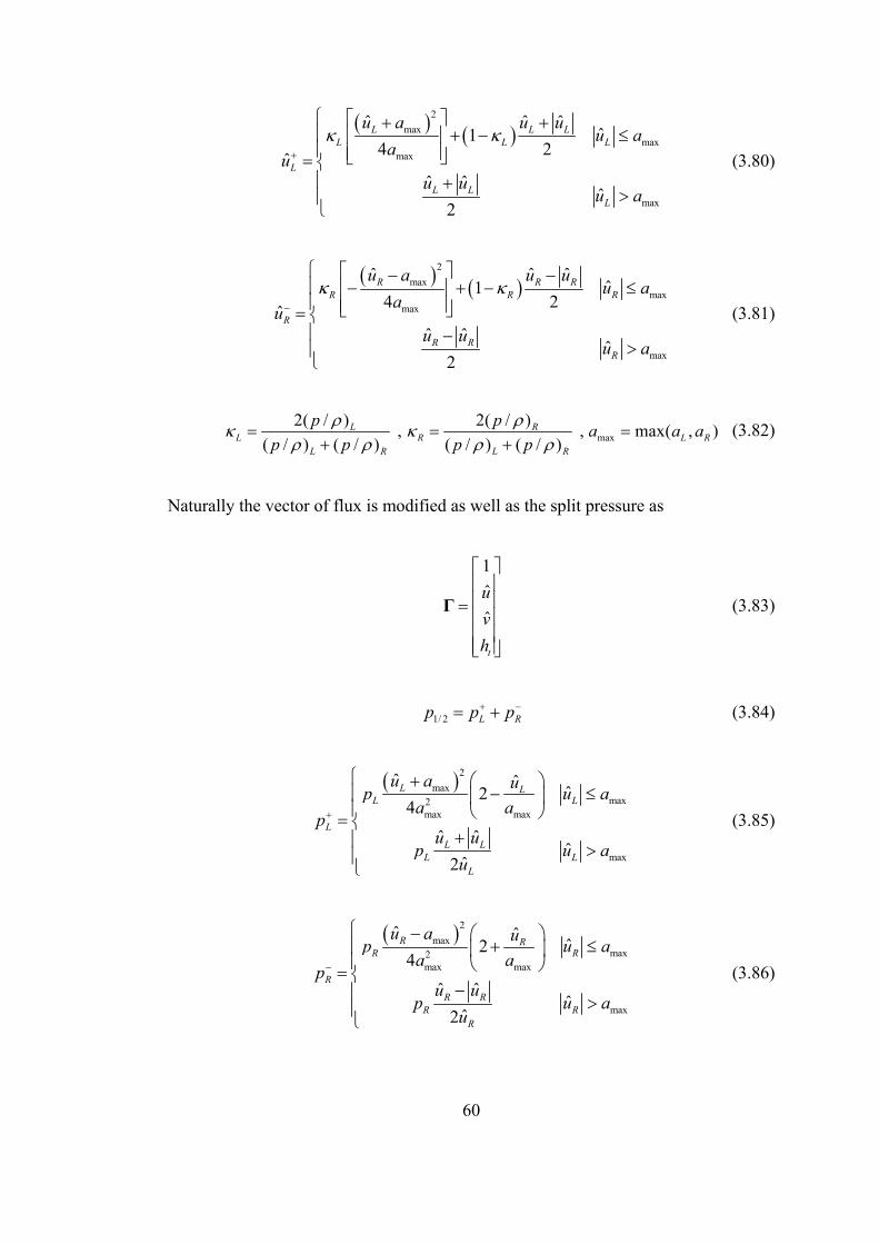
60
( ) ( )2
maxmax
max
max
ˆ ˆˆˆ1
4 2ˆˆ ˆ
ˆ2
L LLL L L
L
L LL
u uu au a
auu u
u a
κ κ+
⎧ ⎡ ⎤ ++⎪ + − ≤⎢ ⎥⎪ ⎢ ⎥⎣ ⎦= ⎨⎪ +
>⎪⎩
(3.80)
( ) ( )2
maxmax
max
max
ˆ ˆˆˆ1
4 2ˆˆ ˆ
ˆ2
R RRR R R
R
R RR
u uu au a
auu u
u a
κ κ−
⎧ ⎡ ⎤ −−⎪ − + − ≤⎢ ⎥⎪ ⎢ ⎥⎣ ⎦= ⎨⎪ −
>⎪⎩
(3.81)
max2( / ) 2( / ), , max( , )
( / ) ( / ) ( / ) ( / )L R
L R L RL R L R
p p a a ap p p p
ρ ρκ κρ ρ ρ ρ
= = =+ +
(3.82)
Naturally the vector of flux is modified as well as the split pressure as
1ˆˆ
t
uvh
⎡ ⎤⎢ ⎥⎢ ⎥=⎢ ⎥⎢ ⎥⎢ ⎥⎣ ⎦
Γ (3.83)
1/ 2 L Rp p p+ −= + (3.84)
( )2max
max2max max
max
ˆ ˆ ˆ24
ˆ ˆˆ
ˆ2
L LL L
L
L LL L
L
u a up u aa a
pu u
p u au
+
⎧ + ⎛ ⎞− ≤⎪ ⎜ ⎟
⎪ ⎝ ⎠= ⎨+⎪ >⎪
⎩
(3.85)
( )2max
max2max max
max
ˆ ˆ ˆ24
ˆ ˆˆ
ˆ2
R RR R
R
R RR R
R
u a up u aa a
pu u
p u au
−
⎧ − ⎛ ⎞+ ≤⎪ ⎜ ⎟
⎪ ⎝ ⎠= ⎨−⎪ >⎪
⎩
(3.86)

61
3.4.4 AUSMV Flux Vector Splitting
Another derivative of the AUSM scheme is the AUSMV flux vector splitting scheme
(22). Similar to the AUSMD scheme the mass flux at the interface of two cells are
estimated as in Equations (3.78) and (3.79) in the AUSMV scheme except for the
normal momentum. The normal momentum is estimated at the interface wholly as
( ) ( ) ( )2
1/ 2ˆ ˆ ˆ ˆ ˆL RL Ru u u u uρ ρ ρ+ −= + (3.87)
The definitions of the split velocities and the pressures differs from the AUSMD
scheme as can be observed from the following equations
( )2ˆˆ
4ˆˆ ˆ
ˆ2
u au a
auu u
u a
±
⎧ ±± ≤⎪⎪= ⎨
±⎪ >⎪⎩
(3.88)
ˆ1 ˆ2ˆ
1 ˆˆ
u u aa ap pu
u au
± ±
⎧ ⎛ ⎞± − ≤⎜ ⎟⎪⎪ ⎝ ⎠= ⋅⎨⎪ >⎪⎩
(3.89)
3.5 Boundary Conditions
The boundary conditions encountered for the external flows considered in the scope
of the thesis work are the solid wall and the far-field boundary conditions. For the
numerical method adopted, the implementation of either type of the boundary
conditions is equivalent to determining the correct right state variables since the left
state variables will always be dictated by the cell under investigation.
For the solid wall, the physical boundary condition is that there is no flux into the
body. In the inviscid case considered, this means that the velocity at the face can be
in the tangential direction.

62
At this point, one of two methods can be adopted for the determination of the right
state variables (14). One is to directly take the flux through the face as zero and to
calculate a right flux solely based on pressure that is equal to the pressure calculated
for the left state. The reason for this equality is that under steady-state conditions, the
pressure force exerted by the fluid will be countered with an equal force. The second
method is to construct a ghost right state for which the tangential velocity, pressure
and total enthalpy are equal to the left state. The direction of the tangential velocity is
the same as the left state as well as the magnitude. For the normal velocity, the
magnitude is equal to that of the left state but the direction is opposite to it. The ghost
right state is depicted for an example cut-cell in Figure 3.3.
Figure 3.3- Ghost right state at the solid wall
The second method ensures zero flux through the face as well but it also takes into
cases where there is a normal velocity component in the presence of high curvatures
as stated in (14). In the code developed, the second method has been adopted for the
solid wall treatment.
For the far-field boundary conditions the right state is calculated from the conditions
received as input and it is irrespective of the left state.
3.6 Reconstruction of the Flow Variables
For the calculation of the fluxes through a face, primitive flow variables have to be
estimated on both sides of that face, the right and left states. The simplest approach
vR
uR
vL
uLhtL htR= htLpL pR= pL
63
would be to take the values from the cell under investigation as the left state and to
take the values from the respective neighbour as the right state. This approach being
first order does not produce very accurate results. Hence it is desirable to reconstruct
the flow variables within the cell to obtain a solution of second order. That is the
variation of the flow variables within the cell must be taken into account even though
in finite volume methods the flow variables representative of the whole cell is stored
at the cell centroid for higher order accuracy.
Three reconstruction schemes have been sighted in the literature. In two of these
three schemes, the gradient of the flow variable is estimated at the centre of the cell
while the other one makes use of finite differences to estimate the value of a flow
variable at certain points within the cell. One of the reconstruction schemes based on
the gradient at the centre of the cell is the Green-Gauss reconstruction, the other one
is the Least Squares (Minimum Energy) reconstruction. The general design criteria
for these reconstruction schemes are discussed in (24) and (25). The details of the
linear reconstruction based on these schemes can be found in (26), (27) and (14)
while the kth order exact schemes are discussed in (28). The third scheme based on
the finite difference method can be found in (29).
3.6.1 Gauss-Green Reconstruction
The Gauss-Green reconstruction is based mainly on the gradient theorem. For a
quantity u related to the cell this can be formulized as
1u undAΩ Ω
∇ = ∫ (3.90)
This integral is evaluated for a region Ω which is bounded by the lines that connect
the centroids of the edge and vertex neighbours (support set) of the cell. The integral
can be evaluated numerically using the trapezoidal rule given as
sup
10
1 1 ( )2
N
i i i iicell
u u u nA +
=
∇ = +∑ (3.91)

64
The boundary of the region Ω is shown for two representative cases for a Cartesian
mesh in Figure 3.4.
Figure 3.4- Region formed by the support set
3.6.2 Least Squares (Minimum Energy) Reconstruction
The Least Squares reconstruction is basically the inverse of the averaging function
for a quantity related to a cell. The average of a quantity u within a cell can be
defined with the averaging function presented as
( ) cellA
cell
udAAv u u
A= =∫
(3.92)
A kth order polynomial uk is constructed to represent the quantity u within the cell
such that the average of the polynomial will be equal to that of the cell and the
polynomial will represent quantity u exactly if u is a polynomial of order k or less. In
general, the constructed polynomial can be obtained as
( )k m n m nmn
m n ku u x y Av x yα
+ ≤
⎡ ⎤= + −⎣ ⎦∑ (3.93)
where mnα are arbitrary coefficients.

65
The form given in Equation (3.93) will ensure that the average of the polynomial is
equal to that of the cell. For a linear case, this reconstruction takes the form presented
in the following equation
[ ] [ ]110 01( , ) c cu x y u x x y yα α= + − + − (3.94)
In Equation (3.94), the centroidal coordinates of the cell appear since by definition
the averaging function applied to the polynomials x and y within the cell gives the
centroid coordinates of the cell.
The reconstruction problem simplifies once the cell average values are thought to be
the values of the flow variables stored at the centroid of the cell (24). Then one could
get the expression of the following form for the linear reconstruction.
[ ] [ ]1( , ) c xc c yc cu x y u u x x u y y= + − + − (3.95)
In Equation (3.95), the only unknowns are uxc and uyc, which are the components of
the gradient of quantity u at the centroid of the cell.
Once the linear polynomial is obtained for the quantity u, the sum of the squares of
the averages of the difference between the value of u obtained from constructed
polynomial and its actual value is minimized within the region made up of the cells
that form the support set to find the unknowns uxc and uyc. The support set is defined
in the same way as the Green-Gauss reconstruction shown in Figure 3.4. This
constitutes the least squares problem for the reconstruction.
sup 21
1( )
N
ii
S Av u u=
⎡ ⎤= −⎣ ⎦∑ (3.96)
0 , 0xc yc
S Su u∂ ∂
= =∂ ∂
(3.97)
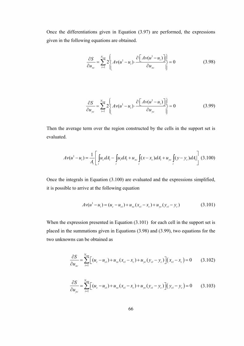
66
Once the differentiations given in Equation (3.97) are performed, the expressions
given in the following equations are obtained.
sup
11
1
( )2 ( ) 0
Ni
iixc xc
Av u uS Av u uu u=
⎧ ⎫⎡ ⎤∂ −∂ ⎪ ⎪⎣ ⎦= − ⋅ =⎨ ⎬∂ ∂⎪ ⎪⎩ ⎭∑ (3.98)
sup
11
1
( )2 ( ) 0
Ni
iiyc yc
Av u uS Av u uu u=
⎧ ⎫⎡ ⎤∂ −∂ ⎪ ⎪⎣ ⎦= − ⋅ =⎨ ⎬∂ ∂⎪ ⎪⎩ ⎭∑ (3.99)
Then the average term over the region constructed by the cells in the support set is
evaluated.
1 1( ) ( ) ( )i c i i i xc c i yc c ii i i i i
Av u u u dA u dA u x x dA u y y dAA⎡ ⎤
− = − + − + −⎢ ⎥⎣ ⎦∫ ∫ ∫ ∫ (3.100)
Once the integrals in Equation (3.100) are evaluated and the expressions simplified,
it is possible to arrive at the following equation
1( ) ( ) ( ) ( )i c ci xc ci c yc ci cAv u u u u u x x u y y− = − + − + − (3.101)
When the expression presented in Equation (3.101) for each cell in the support set is
placed in the summations given in Equations (3.98) and (3.99), two equations for the
two unknowns can be obtained as
( )sup
1( ) ( ) ( ) 0
N
c ci xc ci c yc ci c ci cixc
S u u u x x u y y x xu =
∂ ⎡ ⎤= − + − + − − =⎣ ⎦∂ ∑ (3.102)
( )sup
1( ) ( ) ( ) 0
N
c ci xc ci c yc ci c ci ciyc
S u u u x x u y y y yu =
∂ ⎡ ⎤= − + − + − − =⎣ ⎦∂ ∑ (3.103)

67
Equations (3.102) and (3.103) can be presented in a matrix form as
( )
( )
( )( )
( )( )
sup sup sup
sup sup sup
2
1 1 1
2
1 1 1
( ) ( )
( ) ( )
N N N
ci c ci c ci c ci c ci cxci i i
N N Nyc
ci c ci c ci c ci c ci ci i i
x x x x y y u u x xuu
x x y y y y u u y y
= = =
= = =
⎡ ⎤ ⎡ ⎤− − − − −⎢ ⎥ ⎢ ⎥⎡ ⎤⎢ ⎥ ⎢ ⎥=⎢ ⎥⎢ ⎥ ⎢ ⎥⎣ ⎦⎢ ⎥ ⎢ ⎥− − − − −
⎢ ⎥ ⎢ ⎥⎣ ⎦ ⎣ ⎦
∑ ∑ ∑
∑ ∑ ∑(3.104)
This matrix can be solved to obtain the gradients at the centre of the cell from which
the value of quantity u can be obtained at any location within the cell. The least
squares method is employed for the reconstruction in the code developed.
3.6.3 Gradient Limiting
It is undesirable to introduce new maxima points within the region formed by the
support cells and the cell for which the gradient of flow variables are being
constructed. Hence, the gradients are multiplied by a limiter to avoid introduction of
new maxima points. The linear reconstruction takes the following form with the
application of this condition.
1 ( ) ( )c xc c yc cu u u x x u y y⎡ ⎤= +Φ − + −⎣ ⎦ (3.105)
The value of the limiter Φ is between 0 and 1. To determine the exact value of the
limiter, the maximum and the minimum of the values of quantity u are found at the
cell centroids.
max
minsup
max( , )
min( , ) 1,...,c ic
c ic
u u u
u u u i N
=
= = (3.106)
Then the values of the reconstructed polynomial are evaluated at the corners of the
cell since these locations will have the maximum and minimum values within the cell
for a linear reconstruction. The value of quantity u which deviates the most from the
centroidal value will be marked as 1coru serving as a basis for determining the value

68
of the limiter with the implementation of the formulation given in the following
equation
max1
1
min1
1
1
min 1, 0
min 1, 0
1 0
ccor c
cor c
ccor c
c cor
cor c
u u u uu u
u u u uu u
u u
⎧ ⎛ ⎞−− >⎪ ⎜ ⎟−⎝ ⎠⎪
⎪ ⎛ ⎞−⎪Φ = − <⎨ ⎜ ⎟−⎝ ⎠⎪⎪ − =⎪⎪⎩
(3.107)
3.7 Temporal Discretization
Once the flux terms in the governing Equation (3.8) is obtained, then the temporal
discretization has to be performed to update the values of the conserved quantities. A
multi-stage time stepping method is employed for temporal discretization. A detailed
discussion of the multi-stage methods can be found in (30).
3.7.1 Explicit Time Stepping Schemes
To apply the multi-stage time stepping method, an alternative representation of the
governing Equation (3.8) is employed as
1 0cellt A
∂+ =
∂U R (3.108)
In Equation (3.108), the flux terms are presented in a more compact form as residual
vector, R , and its value can be determined from the known values of the conserved
quantities at a given stage. Hence, Equation (3.108) can be treated as an ordinary
differential equation. This equation can be discretized in m-stages as described in
(31) to obtain the following equation.
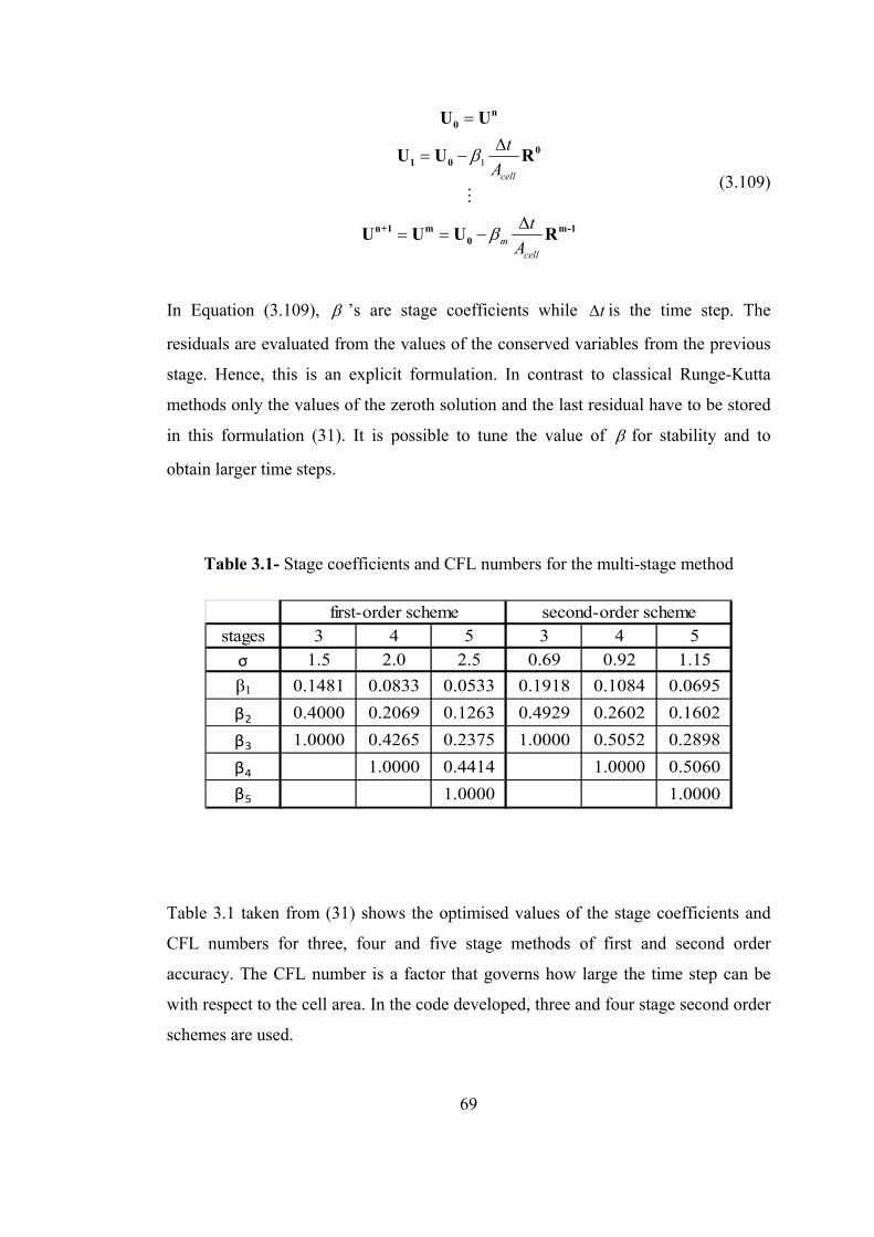
69
1
cell
mcell
tA
tA
β
β
=∆
= −
∆= = −
n0
01 0
n+1 m m-10
U U
U U R
U U U R
(3.109)
In Equation (3.109), β ’s are stage coefficients while t∆ is the time step. The
residuals are evaluated from the values of the conserved variables from the previous
stage. Hence, this is an explicit formulation. In contrast to classical Runge-Kutta
methods only the values of the zeroth solution and the last residual have to be stored
in this formulation (31). It is possible to tune the value of β for stability and to
obtain larger time steps.
Table 3.1- Stage coefficients and CFL numbers for the multi-stage method
stages 3 4 5 3 4 5σ 1.5 2.0 2.5 0.69 0.92 1.15β1 0.1481 0.0833 0.0533 0.1918 0.1084 0.0695β2 0.4000 0.2069 0.1263 0.4929 0.2602 0.1602β3 1.0000 0.4265 0.2375 1.0000 0.5052 0.2898β4 1.0000 0.4414 1.0000 0.5060β5 1.0000 1.0000
first-order scheme second-order scheme
Table 3.1 taken from (31) shows the optimised values of the stage coefficients and
CFL numbers for three, four and five stage methods of first and second order
accuracy. The CFL number is a factor that governs how large the time step can be
with respect to the cell area. In the code developed, three and four stage second order
schemes are used.

70
3.7.2 Determination of the Time Step
In Equation (3.109), the value of the time step is not determined. The value of the
time step, if taken to be too large, will introduce stability problems. If this value is
taken to be too small then the convergence will be very slow and unnecessary
amount of computations will be performed.
The mesh generated for an arbitrary geometry will contain cells that have different
sizes and since the time step is dependent on the cell size, every cell will have a
different maximum time step. As a result, a different time step will be used for each
cell since a steady state solution is sought.
The time step is calculated in terms of the area of the cell under investigation as in
the following formulation given in (31).
x ycell
tA
σ∆=Ψ + Ψ
(3.110)
where σ is the CFL number and Ψ is the spectral radius.
The spectral radii Ψ that appear in Equation (3.110) can be calculated using the
length of the edge projections of the cell in both x-y directions, xS and yS .
( )12
x x
edges
u a SΨ = + ∑ (3.111)
( )12
y y
edgesv a SΨ = + ∑ (3.112)
The time step obtained thus is multiplied by a safety factor in some cases to promote
stable solutions. If Equation (3.110) is investigated, this equation is in one sense a
division of a characteristic length by a characteristic speed. The characteristic speed
is the maximum speed with which information is carried for a cell. Hence, the time

71
step is obtained by constricting the distance information travels from a cell within the
field.
3.8 Solution Refinement
Once a certain level of convergence is achieved, the cells are refined according to the
gradient of the solution. The purpose of this refinement is to provide enough
resolution at the places where there might be discontinuities due to shocks or there
are large gradients in the solution (e.g. around the stagnation point).
The solution refinement criterion used is based on the one outlined in (14). This
method is based on both the curl of the velocity, for detecting shear layers, and the
gradient of the velocity, for detecting shocks. The curl and gradient of the velocity is
multiplied by some characteristic length of the cell as
( ) ( )3 32 2 , =cell cellA V A Vτ ζ= ∇⋅ ∇× (3.113)
The standard deviations of the quantities defined in Equation (3.113) are calculated
and the cells exceeding the standard deviation are refined.
2
1
2
1
Refine cell j
Refine cell j
cell
cell
n
ii
jcell
n
ii
jcell
n
n
τ
ζ
ττ σ
ζζ σ
=
=
⎧ ⎛ ⎞⎪ ⎜ ⎟⎪ ⎝ ⎠> =⎪⎪⎨⎪ ⎛ ⎞⎪ ⎜ ⎟⎪ ⎝ ⎠> =⎪⎩
∑
∑ (3.114)

72
CHAPTER 4
RESULTS &DISCUSSIONS
To test the validity of the code developed, the flow around a NACA0012 airfoil and
an NLR7301 with a flap has been solved for different conditions. Besides
demonstrating the characteristic features of the flows, different methods for handling
the flux terms in the governing equations have been compared.
4.1 NACA0012
The NACA0012 tests have been performed for a subsonic case and a transonic case.
In the subsonic tests the aim is to show the importance of reconstruction to obtain
second order solutions and to discuss the role of first order solution on the stability.
The transonic tests have been performed to demonstrate the shock capturing
capabilities of the various methods used to evaluate the flux terms. Also they are
compared in terms of computational efficiency.
4.1.1 Subsonic Tests
The far-field boundary condition of the first case for the subsonic tests is a free
stream Mach number of 0.6 and an angle of attack of 0˚. The experimental data for
this case can be found in (32) which were extracted from (33). For this case a total of
six runs have been performed. All the runs are performed using Roe’s method. The
convergence criterion for all of the runs is that the standard deviation of the residual
calculated for the continuity equation should drop five levels on a log scale. Two of
the six runs are first order solutions. One of these solutions is with solution
refinement while the other is not. Two runs are performed second order with and

73
without solution refinement, while the last two are run first order until the residuals
drop four levels then they switch to second order.
The pressure coefficient vs. the chord graph for the first order solutions are presented
in Figure 4.1.
Figure 4.1- Cp vs. chord for first order solution
As can be seen from Figure 4.1, the first order solution without solution refinement
performs poorly. It is not possible to catch the peak of the pressure coefficient with
this solution. However, solution refinement introduces a considerable improvement

74
to the solution. But even with solution refinement the peak of the pressure coefficient
graph is not captured accurately.
The pressure coefficient vs. chord graph can also be illustrated for the second order
solution as in Figure 4.2.
Figure 4.2- Cp vs. chord for second order solution
As can be seen from Figure 4.2, the second order solution provides a much more
accurate solution than the first order method as expected. The peak of the pressure
coefficient is captured accurately for both of the solutions with and without solution

75
refinement although the solution with solution refinement is slightly better on this
aspect.
The effect of solution refinement can be illustrated by examining the differences
between a refined and non-refined mesh.
Figure 4.3- A refined and non-refined mesh around stagnation point
In Figure 4.3, the mesh on the right belonging to a solution with refinement has a
considerably denser mesh around the stagnation point than the one without
refinement. This is an expected result since there are large gradients around this
region.
Finally the results obtained with the solution where first order is used until some
convergence is obtained and then it is switched to second order, can be compared
with the fully second order solution.

76
Figure 4.4- Comparison of the second order solutions
In Figure 4.4, it is almost impossible to distinguish between the two solutions. The
same situation also prevails for a solution with refinement. Hence it can be said that
in terms of accuracy there is no difference between the two solutions.
The Mach contours for the second order solution can be depicted as in Figure 4.5.

77
Figure 4.5- Mach contours for NACA0012 subsonic flow
After comparing the first and second order methods in terms of accuracy, their
computational performances can also be compared as in Table 4.1.

78
Table 4.1- Comparison of first and second order solutions
Method Number of Iterations TimeFirst order without refienement 1938 45sec
First order with refienement 2691 2min 37secSecond order without refinement 4325 11min 23sec
Second order with refinement 7490 1hr 1min 36secSwitch to second order without refinement 3236 6min 57sec
Switch to second order with refinement 4425 25min 24sec
Naturally the first order solution converges much faster than the second order
methods, but it would not be reasonable to obtain a solution with this method due to
poor accuracy. As observed from Table 4.1, starting the solutions first order then
switching to second order after some level of convergence, decreases the
computation time considerably compared to full second order solution. Also as
illustrated in Figure 4.4, there is almost no difference between these solutions.
The calculations for the second case of subsonic flow around the NACA0012 airfoil
were performed with a Mach number of 0.4167. By changing the angle of attack
values a lift coefficient vs. angle of attack graph was constructed. To obtain the
solution Roe’s method was used and solution refinement wass not employed.
Since the pressure is the main factor determining the lift force at high speeds, it is
expected to get a good agreement with the experimental data extracted from (34)
until flow separation, a viscosity governed phenomena, is encountered. This
expectation is realized as can be seen from Figure 4.6 within the region where there
is no separation.

79
Figure 4.6- Lift coefficient vs. angle of attack graph
To obtain the results presented in Figure 4.6, first order calculations are performed
until some level of convergence is obtained then the solution is switched to second
order. As discussed earlier this method decreases computation time while there is no
loss in terms of accuracy.
It was also attempted to use a fully second order solution to obtain the results. It was
possible to get solutions within the range of angle of attacks from -6˚ to 8˚. However
for larger angle of attack values than 8˚, divergence in the calculations was observed.
Using the first order solution then switching to second order provided results for
angle of attack values of 10˚, 12˚ and 16˚ also. The results obtained for 12˚ and 16˚

80
are not presented in Figure 4.6 since they are related to a flow with separation and
this case must be treated with a viscous solver. However this fact still indicates that
the first order solution is more stable than the second order one. When the residual
plots for first and second order solutions are investigated, an indication of this fact
can be seen. In Figure 4.7, it is observed that the residuals decrease smoothly for the
first order solution while for the second order one there are a lot of scattering and
oscillations as the residuals decrease.
Figure 4.7- Residual plot for first and second order solutions
By employing the first order method until some level of convergence is obtained, a
first order accurate initialization of the field variables is obtained which eases the

81
convergence of the second order solution. This procedure will be used by default for
the rest of the calculations that will be presented.
4.1.2 Transonic Tests
The far-field conditions for the transonic flow tests around the NACA0012 profile
are a free stream Mach number of 0.85 and an angle of attack of 1˚. For this flow
shocks on the upper and lower surface of the airfoil is expected, the one on the upper
surface being stronger. Each one of the five methods implemented for the evaluation
of the flux terms in the governing equations has been employed in the solution to
compare these methods. The most crucial point in the tests performed is the location
of the shocks. The transonic flow is a more challenging case than the subsonic flow.
Hence the performance of different methods to evaluate the flux terms is compared
for this case. The calculations have been performed both with and without solution
refinement. To verify the computational solution, AGARD data (35) has been
extracted from (14).
To compare the accuracy of the different methods for evaluating the fluxes,
calculations with solution refinement have been performed. First the results obtained
from the AUSM and its derivative methods are compared amongst themselves. The
pressure coefficient vs. the chord graph for these methods is illustrated in Figure 4.8.

82
Figure 4.8- Pressure coefficient vs. chord graph for the AUSM methods
It is observed from Figure 4.8 that the AUSMD and AUSMV methods capture the
location of the weaker shock on the lower surface while the AUSM predicts this
location slightly downstream. On the upper surface none of the methods were able to
capture the shock location exactly. The AUSMD and the AUSMV methods provide a
closer estimation of the shock location on this surface than the AUSM method. All of
the methods exhibit oscillations around the shock location, the ones on the upper
surface being more marked. This is due to the performance of the limiter in the
calculation of the fluxes.

83
The Roe’s method and the van Leer method can be compared with one of the
representative AUSM methods. The AUSMV method providing the most accurate
results among the AUSM methods is chosen as the representative AUSM method
and the pressure coefficient vs. chord graph for these methods is illustrated in Figure
4.9.
Figure 4.9- Pressure coefficient vs. chord graph for Roe, van Leer and AUSMV
It is seen that both the Roe’s method and the van Leer’s method estimate the shock
location at a slightly upstream position on the upper surface while there is good
agreement on the lower surface. The oscillations around the shock locations are also

84
inherent in these methods. In terms of accuracy AUSMD, AUSMV and the van
Leer’s methods provide the best results for this particular test case.
Besides the accuracy of the methods, their convergence characteristics should also be
examined. The convergence criterion is that the residual for the continuity equation
calculated in the first step should drop five levels on a log scale. None of the methods
were able to provide a five level drop in the residual for solution adaptive
calculations. Hence to compare the convergence characteristics calculations without
solution refinement have been performed. The calculations were performed with four
different CFL safety coefficients; 1.0, 0.5, 0.2 and 0.1, four each one of the five
methods. In Table 4.2, the results for the solution with the maximum CFL safety
factor providing a convergent solution has been presented.
Table 4.2- Computational characteristics of the methods for evaluating fluxes
Method Convergence Number of Iterations Calculation Time CFL Safety CoefficientAUSM converges 5555 9min 1sec 1.0
AUSMD oscillates 100000 3hr 35min 4sec 0.1AUSMV converges 9646 16min 19sec 0.5
Roe converges 5207 9min 15sec 1.0van Leer diverges - - -
The AUSM and the Roe’s methods converged with a CFL safety coefficient of 1.0
while the AUSMV method converged with a CFL safety factor of 0.5. For the
AUSMD method with a CFL safety factor of 0.1, the residual of the continuity
equation oscillates around 8x10⁻⁴ corresponding to a residual drop of about four
levels after about 60000 steps till the maximum number of iterations of 100000. The
van Leer method diverges when solution refinement is not applied implying a
relation between the method and the mesh size. The residual plots for the convergent
solutions can be depicted as in Figure 4.10.

85
Figure 4.10- Residual plot for transonic flow
It is also possible to show the effect of solution adaptation on the mesh generated
initially. The solution refinement has been performed every time the residuals
dropped to one twentieth of the initial residual which is updated just before solution
adaptation is performed. The effect of mesh generation in the critical regions around
the airfoil is illustrated in Figure 4.11.

86
Figure 4.11- Effect of refinement at shock location
As can be seen from Figure 4.11, the mesh is refined around the location of the shock
since there are large gradients in the flow variables at this location. Another region
where large gradients are observed is at the nose of the airfoil around the stagnation
point. The effect of solution refinement in this region is illustrated in Figure 4.12.
Figure 4.12- Effect of refinement around stagnation point
The effect of solution adaptation can be illustrated by plotting the Mach contours for
a refined and non-refined solution.

87
Figure 4.13- Mach contours for transonic flow around NACA0012 airfoil
In Figure 4.13, the Mach contours obtained with the AUSMV method are displayed.
As can be observed for the solution without refinement, the shocks are smeared. The
pressure coefficient vs. chord graphs of these solutions can also be displayed. In
Figure 4.14, it is seen that the solution obtained without refinement is able to capture
both the pressure distribution on the airfoil and the shock locations with refinement
introducing a slight improvement on both aspects. However in Figure 4.13, it is seen
that the overall flow field is not represented accurately without solution refinement.
Hence it can be said that if the main concern is obtaining the forces on the airfoil, the
solution without refinement will provide a good estimation in a considerably shorter
amount of time.

88
Figure 4.14- Pressure coefficient vs. chord for AUSMV with and without refinement
4.2 NLR 7301 with Flap
The NLR 7301 tests have been performed for a gap of 2.6% percent of chord length,
an overlap of 5.3% of chord length and a flap angle of 20˚. The definition of these
variables can be shown as in Figure 4.15.

89
Figure 4.15- Definition of geometry variables for NLR 7301 with flap
Tests were performed at three different angle of attack values; 6˚, 10.1˚ and 13.1˚.
The free stream Mach number for all the cases was 0.185. The five methods; Roe,
van Leer, AUSM, AUSMD, AUSMV, have been employed in the calculations. To
verify the results computed, data obtained from (36) has been used.
The pressure coefficient vs. chord graph for angle of attack of 6˚ is presented for the
AUSM methods in Figure 4.16. All of the AUSM methods are able to capture
pressure distribution with good accuracy for the most part. But in terms of capturing
the peak of the pressure coefficient on the upper surface of the main airfoil, AUSM
method is superior to the others. The AUSMD method performs better than the
AUSMV method on this aspect.
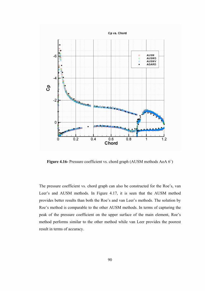
90
Figure 4.16- Pressure coefficient vs. chord graph (AUSM methods AoA 6˚)
The pressure coefficient vs. chord graph can also be constructed for the Roe’s, van
Leer’s and AUSM methods. In Figure 4.17, it is seen that the AUSM method
provides better results than both the Roe’s and van Leer’s methods. The solution by
Roe’s method is comparable to the other AUSM methods. In terms of capturing the
peak of the pressure coefficient on the upper surface of the main element, Roe’s
method performs similar to the other method while van Leer provides the poorest
result in terms of accuracy.

91
Figure 4.17- Pressure coefficient vs. chord graph (AUSM, Roe, van Leer AoA 6˚)
The computational performances of each method can be tabulated to obtain a
comparison.

92
Table 4.3- Computational performance of the methods for NLR 7301 AoA 6˚
Method Convergence Number of Iterations Time Lift CoefficientAUSM converges 7072 41min 47sec 2.51
AUSMD oscillates 100000 10hr 21min 49sec 2.46AUSMV oscillates 100000 10hr 14min 0sec 2.45
Roe oscillates 100000 10hr 56min 15 sec 2.42van Leer converges 4172 22min 53sec 2.35
It is observed from Table 4.3 that the van Leer’s method converges faster than the
AUSM method. The other methods; AUSMD, AUSMV and Roe, do not converge,
that is the residuals in the continuity equation do not drop five levels but they
fluctuate until the maximum number of iterations is reached. Also it can be seen that
the highest lift coefficient is found with the AUSM method. This is an expected
result as the AUSM method captures the peak of the pressure distribution on the
upper surface of the main airfoil better than the other methods. The AUSMD,
AUSMV and Roe’s methods provide a similar result on this aspect while van Leer’s
method gives the smallest estimate as it was the worst in capturing the peak.
The pressure coefficient vs. chord graph for the angle of attack value of 10.1 can be
presented for the AUSM methods. From Figure 4.18, it is seen that the performance
of the AUSM method is better than both the AUSMD and the AUSMV methods. The
AUSMV method starts to deviate from the AGARD data which is especially
apparent on the upper surface of the flap. The peak of the pressure coefficient is
captured accurately with the AUSM method.

93
Figure 4.18- Pressure coefficient vs. chord graph (AUSM methods AoA 10.1˚)
The pressure coefficient vs. the chord graph can be presented for the AUSM, Roe
and van Leer methods as in Figure 4.19.

94
Figure 4.19- Pressure coefficient vs. chord graph (AUSM, Roe, van Leer AoA 10.1˚)
As can be seen from Figure 4.19, AUSM method provides a better solution. It is also
observed that the Roe’s method provides a better estimation of the peak in the
pressure distribution on the upper surface of the main element than the AUSMD and
AUSMV methods.
The computational performance of the methods can also be compared from Table
4.4.

95
Table 4.4- Computational performance of the methods for NLR 7301 AoA 10.1˚
Method Convergence Number of Iterations Time Lift CoefficientAUSM converges 11567 1hr 10min 43sec 2.98
AUSMD oscillates 100000 10hr 21min 5sec 2.76AUSMV oscillates 100000 10hr 13min 2sec 2.75
Roe converges 78924 8hr 15min 47 sec 2.86van Leer converges 4175 22min 50sec 2.83
It is observed from Table 4.4 that as the angle of attack is increased Roe’s method
converges like the AUSM and the van Leer methods. The performances of the van
Leer, AUSMD and AUSMV methods essentially remain the same computationally.
The Roe’s method being able to capture the pressure peak better for this case,
estimates a relatively higher lift coefficient than the previous case. The AUSM
method still being the best one to capture the peak provides the highest estimate of
the lift coefficient.
The pressure coefficient vs. the chord graph can be constructed for the angle of
attack of 13.1˚ for the AUSM methods. From Figure 4.20, it is seen that the AUSMV
method fails at this angle of attack. Once again the AUSM method provides a
considerably better estimate of the pressure peak on the upper surface of the main
element.

96
Figure 4.20- Pressure coefficient vs. chord graph (AUSM methods AoA 13.1˚)
In Figure 4.21 the pressure coefficient vs. chord graph for the AUSM, Roe and van
Leer methods are depicted. The AUSM method providing the best of the solutions,
the Roe’s method provides a better solution than van Leer’s method. As in the case
of angle of attack of 10.1˚, the Roe’s method gives a better solution than the
AUSMD and AUSMV method which fails.

97
Figure 4.21- Pressure coefficient vs. chord graph (AUSM, Roe, van Leer AoA 13.1˚)
The computational performance of the methods for the case of angle of attack of
13.1˚ can be compared with the aid of Table 4.5.

98
Table 4.5- Computational performance of the methods for NLR 7301 AoA 13.1˚
Method Convergence Number of Iterations Time Lift CoefficientAUSM converges 12182 1hr 14min 5sec 3.29
AUSMD oscillates 100000 10hr 20min 30sec 3.08AUSMV oscillates 100000 10hr 13min 5sec 3.03
Roe converges 87222 9hr 11min 9sec 3.17van Leer converges 4396 24min 12sec 3.16
The computational performance of the methods is pretty similar to the case of angle
of attack of 10.1˚ with the exception that AUSMV method fails totally. It can be
concluded that AUSM method provides the best results in all the cases considered.
Roe’s and van Leer’s methods do improve as the angle of attack increases which
may be due to the fact that as the angle of attack increases so does the velocities
around the airfoil, which makes the problem shift closer to the compressible range.
The performance of the AUSMD method remains constant while the AUSMV
method fails as the angle of attack is increased.
Solution adaptive calculations have also been performed for the van Leer method to
improve the results. The effect of solution refinement on the mesh can be shown as
in Figure 4.22 and Figure 4.23.

99
Figure 4.22- Effect of solution refinement around stagnation region of NLR 7301
Figure 4.23- Effect of solution refinement around the flap

100
The pressure coefficient vs. the chord graphs for the solution with and without
refinement can be constructed for a comparison at 6˚.
Figure 4.24- Pressure coefficient vs. chord for van Leer AoA 6˚
In Figure 4.24, it is seen that the adapted solution performs better at capturing the
peak of the pressure distribution on the upper surface of the main element. In fact the
solution is improved around this region as a whole. The estimate of the lift
coefficient increases from 2.35 to 2.49. This is much closer to the one predicted by
the AUSM method.

101
The pressure coefficient vs. the chord graph for a solution with and without
refinement for angle of attack of 10.1˚ is presented in Figure 4.25.
Figure 4.25- Pressure coefficient vs. chord for van Leer AoA 10.1˚
There is an overall improvement of the solution with the introduction of refinement,
but this time there is a considerable over estimation of the peak of the pressure
coefficient on the upper surface of the main element. In fact the estimation for the lift
coefficient becomes 3.05 which is greater than predicted by the AUSM method.
Lastly, the pressure coefficient vs. the chord graph for a solution with and without
refinement for angle of attack of 13.1˚ is presented in Figure 4.26.

102
Figure 4.26- Pressure coefficient vs. chord for van Leer AoA 13.1˚
Once again the overall solution does improve, but there is an over prediction of the
pressure coefficient peak on the upper surface of the main element.
Figure 4.27, Figure 4.28 and Figure 4.29 illustrate the flow fields obtained for angle
of attack values of 6˚, 10.1˚, 13.1˚ respectively.

103
Figure 4.27- Flow field for NLR 7301 with flap AoA 6˚
Figure 4.28- Flow field for NLR 7301 with flap AoA 10.1˚

104
Figure 4.29- Flow field for NLR 7301 with flap AoA 13.1˚
As the angle of attack increases, the acceleration of the flow on the upper surface of
the main element increases also. This makes the streamlines more compact, and also
the pressure drop on the upper surface of the main element increases. In addition,
with the increasing angle of attack the region of high pressure on the lower surface of
the main element becomes larger. This promotes higher lift forces, which is
consistent with the computations. An important feature of the NLR 7301 airfoil is the
region between its lower surface and the flap. There were no vortex formations in
this region for the flows considered. If there were a vortex formation in this region,
due to the pressure drop associated with it, there would be decrease in the lift force
accompanied by an increase in the drag force since the orientation of the face normal

105
of the main element is towards increasing the lift and decreasing the drag in this
region. Hence viscous calculations are of great importance in this region because of a
possibility of separation.

106
CHAPTER 5
CONCLUSIONS
In the subsonic calculations, the difference between the accuracy of a first order and
a second order formulation has been illustrated. The first order method is inadequate
in capturing the flow characteristics such as the peak of the pressure distribution for
the relatively simple problem of subsonic flow. There is however a considerable
improvement of the solution with the introduction of solution refinement. This is due
to the fact that with solution refinement, the mesh around the regions of high
gradients, the stagnation region in case of NACA0012 subsonic flow, is refined and
the accuracy in this region increases as the peak of the pressure distribution can be
captured more accurately.
Even though solution refinement did introduce an improvement on the first order
solution, it still wasn’t accurate enough. The second order method performed much
better than a first order solution with refinement. When solution refinement was
performed for a second order formulation, there was little improvement in the
solution for NACA0012 subsonic flow, since the non-adapted solution performed
reasonably well, to capture the peak of the solution refinement.
The second order method was superior to the first order one in terms of accuracy, but
it did call for a much increased computation time. To resolve this issue, first order
calculations would be performed until some level of convergence is obtained then the
solution would switch to a second order formulation. This resulted in up to more than
50% decrease in the computation time while there was no virtual loss in terms of
accuracy. Also as the angle of attack was varied to construct a lift coefficient vs.
chord graph it was seen that at certain angles it was not possible to get a solution
with fully second order calculations. This and the fact that second order solutions

107
provided residual plots with considerable scattering and oscillations indicated that
the first order formulation is more stable than the second order one. Hence by
starting with first order calculations, the field is initialized more accurately which
promotes the second order method to converge as it is sensitive to the initial
conditions.
The transonic flow around the NACA0012 profile was a more challenging case than
the subsonic flow, providing grounds to test the performance of different methods for
evaluating the flux terms. The main challenge was to catch the shock locations,
especially the stronger one on the upper surface of the airfoil. The AUSMD,
AUSMV and van Leer’s methods were the ones that showed the best performance on
this aspect.
For the transonic flow solution refinement is a must to get an accurate representation
of the flow field since it is already known that there will be large gradients at shock
locations in addition to the stagnation region. If solution refinement is not used
smeared shocks are obtained. It was however possible to get an accurate pressure
distribution on the airfoil as the mesh elements in this region are small in size. Hence
just to analyze the forces on the airfoil a solution without refinement can be
employed to get quick results.
It was not possible to compare the computational performance of the methods with a
solution with refinement, so calculations were also performed without refinement.
For the solutions without refinement it was seen that, the Roe’s method and the
AUSM method converged easily with a CFL safety coefficient of 1. The AUSMV
method converged with a CFL safety coefficient of 0.5 while the van Leer’s method
diverged.
Another important feature of the solutions for the transonic flow was the oscillations
seen at the shock locations, the one on the upper surface of the airfoil with the
stronger shock being more apparent. This is due to the poor performance of the
limiters used in the calculations. A limiter that won’t hamper the convergence while
preventing oscillations should be implemented to improve the solution.

108
The NLR 7301 with a flap was also a challenging case to test the performance of the
various methods implemented for evaluating the flux terms. The AUSM method was
superior in terms accuracy and it was second to van Leer’s method in terms of
computational performance. The van Leer’s method with the poorest performance for
the case with an angle of attack of 6˚ did improve with the application of solution
refinement.
The performance of both the Roe’s and van Leer’s methods improved for the cases
with higher angle of attacks. This might be due to the flow shifting closer to the
compressible range with the increasing angle of attacks promoting higher velocities
in the field. The performance of the AUSMD method was consistent throughout the
calculations while the AUSMV method failed for large angle of attack values.
From the pressure coefficient vs. chord graphs, it was observed that the estimation of
the peak pressure on the upper surface of the main element was crucial in the
prediction of the lift coefficient. van Leer’s method with solution refinement and
AUSM method performed well on this aspect, while AUSMD, AUSMV, and Roe’s
method performed worse with similar results at an angle of attack 6˚. For the angle of
attack values of 10.1˚ and 13.1˚, AUSM was the superior method once again while
the performance of Roe’s method improved considerably. The van Leer method with
solution refinement provided over estimations of the pressure peak.

109
BIBLIOGRAPHY
1. Wendt, John F, et al. Computational Fluid Dynamics An Introduction. Berlin :
Springer_Verlag, 1996.
2. Versteeg, H K and Malalasekera, W. An Itroduction to Computational Fluid
Dynamics The Finite Volume Method. Malaysia : Prentice Hall, 1995.
3. Liseikin, Vladimir D. Grid Generation Methods. Berlin : Springer-Verlag, 1999.
4. Thompson, Joe F, Soni, Bharat K and Wheatherill, Nigel P. Handbook of Grid
Generation : CRC Press, 1998.
5. Hirsch, Charles. Numerical Computation of Internal and External Flows. New
York : John Wiley & Sons, 1988.
6. Reddy, J N. An Introduction to the Finite Element Method. Singapore : McGraw-
Hill, 1993.
7. Hoffmann, Klaus A and Chiang, Steve T. Computational Fluid Dynamics for
Engineers. Wichita : Enginnering Education System, 1995.
8. Reentrant Polygon Clipping. Sutherland, I E and Hodgeman, G W. January
1974, Communications of the ACM, pp. 32-42.
9. A New Concept and Method for Line Clipping. Liang, Y D and Barsky, B A. 1,
January 1984, ACM Transactions on Graphics, Vol. 3, pp. 1-22.
10. Sproull, R F and Sutherland, I E. A Clipping Divider. Washington D. C. :
Thompson Books, 1968.

110
11. An Efficent Algorithm for 2-D Line Clipping: Its Development and Analysis.
Nicholl, Tina M, Lee, D T and Nicholl, Robin A. July 1987, Computer Graphics,
pp. 253-262.
12. A New Two Dimensional Line Clipping Algorithm for Small Windows. Day, J D.
1992, Computer Graphic Forums, pp. 241-245.
13. A Fast Two-Dimensional Line Clipping Algoritm via Line Encoding. Sobkow, M
S, Pospisil, P and Yang, Y H. 1987, Computer Graphics, pp. 459-467.
14. De Zeeuw, Darren L. A Quad-Tree Based Adaptively-Refined Cartesian-Grid
Algorithm for the Solution of The Euler Equations. Michigan : The University of
Michigan, 1993. PhD thesis.
15. Preparata, P Franco and Shamos, Michael Ian. Computational Geometry an
Introduction. New York : Springer-Verlag, 1985.
16. Toro, E F. Riemann Solvers and Numerical Methods for Fluid Dynamics.
Berlin : Springer-Verlag, 1999.
17. Laney, Culbert B. Computational Gas Dynamics. Cambridge : Cambridge
University Press, 1998.
18. Greenberg, Michael D. Advanced Engineering Mathematics. New Jersey :
Prentice Hall, 1998.
19. Approximate Riemann Solvers, Parametrized Vectors, and Difference Schemes.
Roe, P L. 1981, Journal of Computational Physics, Vol. 43, pp. 357-372.
20. Flux Vector Splitting for the Euler Equations. van Leer, B. s.l. : Springer-Verlag,
1982. Proceedings of the 8th International Conference on Numerical Methods in
Fluid Dynamics.

111
21. A New Flux Splitting Scheme. Liou, M S and Steffen, C J. s.l. : Journal of
Computational Physics, 1993, Vol. 107, pp. 23-39.
22. An Accurate and Robust Vector Splitting Scheme for Shock and Contact
Discontinuities. Wada, Yasuhiro and Liou, M S. 3, s.l. : Siam J. Sci. Comput.,
1997, Vol. 18, pp. 633-657.
23. Flux Vector Splitting of the Inviscid Gasdynamic Equations with Applications to
Finite Difference Methods. Steger, J L and Warming, R F. s.l. : Journal of
Computational Physics, 1981, Vol. 40, pp. 263-293.
24. Barth, Timothy J. Simplified Numarical Methods for Gasdynamic Systems on
Triangulated Domains. Stanford : Stanford University, 1998. PhD thesis.
25. Barth, Timothy J and Frederickson, Paul O. Higher Order Solution of the
Euler Equations. Reno : AIAA paper AIAA-90-0013, 1990. 28th Aerospace
Sciences Meeting.
26. Barth, Timothy J and Jespersen, Dennis C. The Design and Application of
Upwind Schemes on Unstructured Meshes. Reno : AIAA paper AIAA-89-0366,
1989. 27th Aerospace Sciences Meeting.
27. Coirier, William John. An Adaptively Refined, Cartesian, Cell-Based Scheme
for the Euler and Navier Stokes Equations. Michigan : The University of Michigan,
1994. PhD thesis.
28. Barth, Timothy J. Recent Developments in High Order K-Exact Reconstruction
on Unstructured Meshes. Reno : AIAA paper AIAA-93-0668, 1993. 31st Aerospace
Sciences Meeting.
29. Gerris: A Tree-Based Adaptive Solver for the Incompressible Euler Equations in
Complex Geometries. Popinet, Stéphane. 2003, Journal of Computational Physics,
Vol. 190, pp. 572-600.

112
30. Lambert, J D. Computational Methods in Ordinary Differential Methods.
London : Wiley, 1973.
31. Blazek, J. Computational Fluid Dynamics: Principles and Applications. St
Augustin : Elsevier, 2001.
32. Amick, J L. Comparison of the Experimental Pressure Distribution on an
NACA0012 Profile at High Speeds with that Calculated by the Relaxation Method.
s.l. : National Advisory Committee for Aeronautics, 1950. Technical note.
33. Özdemir, Enver Doruk. Implementation of Rotation into a 2-D Euler Solver.
Ankara : METU, 2005. Masters thesis.
34. Abbott, Ira H and von Doenhoff, Albert E. Theory of Wing Sections,Including
a Summary of Airfoil Data. New York : Dover Publications, 1959.
35. AGARD Subcommittee C. Test Cases for Inviscid Flow Field Methods. 1986 :
AGARD Advisory Report 211.
36. Advisory Group for Aerospace Research& Development. A Selection of
Experimental Test Cases for the Validation of CFD Codes . s.l. : AGARD Advisory
Report No 303, 1994.

113
APPENDIX A
COORDINATES OF NACA0012
Table A.1- Coordinates of NACA0012 Profile
x y0.999753 0.0012950.999013 0.0013980.997781 0.0015710.996057 0.0018120.993844 0.0021200.991144 0.0024960.987958 0.0029370.984292 0.0034430.980147 0.0040120.975528 0.0046420.970440 0.0053330.964888 0.0060820.958877 0.0068870.952414 0.0077460.945503 0.0086580.938153 0.0096190.930371 0.0106280.922164 0.0116810.913540 0.0127780.904508 0.0139140.895078 0.0150880.885257 0.0162970.875056 0.0175390.864484 0.0188090.853553 0.0201070.842274 0.0214290.830656 0.0227730.818712 0.024135

114
Table A.1- Coordinates of NACA0012 Profile (continued)
0.806454 0.0255140.793893 0.0269050.781042 0.0283070.767913 0.0297170.754521 0.0311310.740877 0.0325470.726995 0.0339620.712890 0.0353740.698574 0.0367780.684062 0.0381720.669369 0.0395530.654508 0.0409170.639496 0.0422630.624345 0.0435850.609072 0.0448820.593691 0.0461490.578217 0.0473830.562667 0.0485810.547054 0.0497390.531395 0.0508540.515705 0.0519230.500000 0.0529400.484295 0.0539040.468605 0.0548100.452946 0.0556550.437333 0.0564360.421783 0.0571480.406309 0.0577890.390928 0.0583550.375655 0.0588440.360504 0.0592510.345492 0.0595750.330631 0.0598120.315938 0.0599600.301426 0.0600170.287110 0.0599800.273005 0.0598480.259123 0.0596190.245479 0.0592920.232087 0.058866

115
Table A.1- Coordinates of NACA0012 Profile (continued)
0.218958 0.0583400.206107 0.0577140.193546 0.0569870.181288 0.0561600.169344 0.0552330.157726 0.0542070.146447 0.0530830.135516 0.0518630.124944 0.0505470.114743 0.0491380.104922 0.0476380.095492 0.0460490.086460 0.0443740.077836 0.0426150.069629 0.0407760.061847 0.0388590.054497 0.0368670.047586 0.0348030.041123 0.0326710.035112 0.0304730.029560 0.0282130.024472 0.0258930.019853 0.0235170.015708 0.0210880.012042 0.0186070.008856 0.0160780.006156 0.0135030.003943 0.0108840.002219 0.0082230.000987 0.0055210.000000 0.000000

116
APPENDIX B
COORDINATES OF NLR 7301 & FLAP
Table B.1- The coordinates of NLR 7301
x y0.94360 0.014990.94267 0.015190.93988 0.015800.93524 0.016900.92878 0.018300.92051 0.020080.91047 0.022410.89870 0.025120.88524 0.028190.87015 0.031620.85349 0.035360.83532 0.039410.81572 0.043680.79476 0.048140.77253 0.052730.74911 0.057350.72459 0.061910.69908 0.066280.67267 0.070380.64547 0.074100.61758 0.077370.58912 0.080150.56019 0.082480.53092 0.084380.50141 0.085900.47178 0.087040.44216 0.087810.41265 0.088260.38337 0.088380.35444 0.088180.32598 0.08768

117
Table B.1- The coordinates of NLR 7301 (continued)
0.29809 0.086870.27098 0.085770.24448 0.084400.21897 0.082760.19445 0.080870.17103 0.078740.14880 0.076380.12784 0.073810.11786 0.072450.10824 0.071030.09897 0.069580.09007 0.068070.08155 0.066500.07341 0.064880.06567 0.063170.05832 0.061370.05139 0.059430.04487 0.057310.03877 0.055060.03309 0.052680.02786 0.050090.02305 0.047170.01870 0.043730.01479 0.039780.01133 0.035440.00832 0.030760.00577 0.025820.00368 0.020640.00206 0.015160.00089 0.009590.00019 0.00422-0.00004 -0.000800.00019 -0.005520.00089 -0.009920.00206 -0.014170.00368 -0.018040.00577 -0.021730.00832 -0.025210.01133 -0.028510.01479 -0.031580.01870 -0.03445

118
Table B.1- The coordinates of NLR 7301 (continued)
0.02305 -0.037170.02786 -0.039720.03310 -0.042150.03877 -0.044430.04487 -0.046610.05139 -0.048730.05832 -0.050730.06567 -0.052630.07341 -0.054460.08155 -0.056220.09007 -0.057910.09897 -0.059540.10824 -0.061090.11786 -0.062590.12784 -0.064020.14880 -0.066720.17103 -0.069170.19445 -0.071320.21897 -0.073170.24448 -0.074700.27089 -0.075850.29809 -0.076660.32598 -0.077040.35444 -0.077010.38337 -0.076520.41265 -0.075500.44216 -0.073850.47178 -0.071440.50141 -0.068190.53092 -0.064170.56019 -0.059590.58912 -0.054590.61758 -0.049210.64547 -0.043550.67267 -0.037500.69908 -0.030800.72459 -0.023620.74911 -0.015970.77253 -0.008240.79476 -0.000800.81572 0.00585

119
Table B.1- The coordinates of NLR 7301 (continued)
0.83532 0.011150.85349 0.014720.87015 0.017020.88524 0.018180.89870 0.018430.91047 0.018070.92051 0.017330.92878 0.016450.93524 0.015300.93988 0.014600.94267 0.014230.94360 0.01410
Table B.2- The coordinates of flap
x y1.205092 -0.1021331.204014 -0.1014111.200754 -0.0993731.195420 -0.0959311.188106 -0.0910561.178790 -0.0852491.167564 -0.0787261.154588 -0.0716621.140013 -0.0642821.124077 -0.0566941.106992 -0.0491351.098093 -0.0454281.088996 -0.0417981.079729 -0.0382861.070330 -0.0349291.060832 -0.0317281.051260 -0.0287011.041673 -0.0258611.032094 -0.0232051.022570 -0.020749

120
Table B.2- The coordinates of flap (continued)
1.013137 -0.0185081.003821 -0.0165320.994643 -0.0148200.985653 -0.0134100.976874 -0.0122690.968366 -0.0114070.960148 -0.0107990.952264 -0.0104730.944743 -0.0104070.937624 -0.0105830.930955 -0.0109220.924783 -0.0113900.919139 -0.0119850.914029 -0.0127220.909442 -0.0136590.905415 -0.0148120.901946 -0.0161560.899047 -0.0177190.896720 -0.0195220.895009 -0.0214740.893925 -0.0235170.893589 -0.0253740.893925 -0.0271990.894976 -0.0289010.896887 -0.0300540.899614 -0.0307490.903046 -0.0312320.907107 -0.0317410.911738 -0.0323200.916920 -0.0329930.922644 -0.0337570.928889 -0.0345820.935621 -0.0354690.942821 -0.0364180.950452 -0.0374400.958495 -0.0385260.966901 -0.0396700.975646 -0.0409060.984677 -0.0422030.993974 -0.043586

121
Table B.2- The coordinates of flap (continued)
1.003479 -0.0450451.013157 -0.0466091.022976 -0.0482571.032883 -0.0500111.042829 -0.0518651.052791 -0.0538201.062706 -0.0558751.072539 -0.0580381.082262 -0.0603001.091824 -0.0626521.101185 -0.0650911.119166 -0.0701881.135943 -0.0754651.151267 -0.0807871.164948 -0.0859151.176820 -0.0906621.186673 -0.0949931.194459 -0.0985721.200104 -0.1011591.203556 -0.1026701.204699 -0.103214