a two-methodology comparison study of a spatial gravity

A Two-Methodology Comparison Study of a Spatial Gravity Model in the Context

of Interregional Trade Flows

Autores y e-mail de la persona de contacto:

Luisa Alamá-Sabater*

Laura Márquez-Ramos*

Email:[email protected]

José Miguel Navarro-Azorín**

Celestino Suárez-Burguet*

Departamento:

Departamento de Economía

Universidad: *Universitat Jaume I, Castellón, Spain ** Universidad Politécnica de Cartagena, Spain

Área Temática: movilidad, transporte e infraestructuras

Resumen: (máximo 300 palabras)

This paper argues that the introduction of spatial interactions to model the determinants

of origin-destination (OD) flows can potentially result in excessive contiguity. To

explain flows between OD regions, it is not only what happens in the origin and

destination that is relevant, but also what happens in their neighbouring regions.

However, what happens if there is a high degree of overlap between origin neighbouring

areas and destination neighbouring areas? The paper presents an empirical illustration to

re-examine the evidence presented in previous research (Alamá-Sabater et al., 2013)

and more closely analyses the territorial level, focusing on the case of interregional

trade of goods at the NUTS3 level (Spanish provinces). We then use two different

methodologies within the framework of a spatial gravity equation for interregional trade

modelling. The findings confirm the importance of spatial dependence on trade flows

and in particular that logistics decisions within a province affect shipments from

contiguous provinces.

Palabras Clave: (máximo 6 palabras)

gravity, spatial dependence, connectivity, interregional trade, Spanish provinces

Clasificación JEL: F14, R12

1. Introduction

The link between spatial dependence and trade flows stems from contributions made by

LeSage and Pace (2004; 2008). LeSage and Polasek (2008) and LeSage and Thomas-

Agnan (2014) introduce spatial effects into the econometric flow model, which can be

interpreted as an extension of OD models used in the international trade literature: the

gravity equation. In particular, these authors redefine the concept of spatial effects by

considering the idea that the relation between OD flows depends not only on the

features of origin and destination, as in a traditional gravity equation, but also on the

characteristics of neighbouring regions. These characteristics can be measured by the

flows between the neighbouring regions and the origin or destination regions.

This paper contributes to the existing literature in two ways. First, it explores the

empirical performance of the gravity model to explain trade flows between regions

using a spatial approach. To do so, it employs two different methodologies. The first

methodology extends the gravity model controlling for the so-called multilateral

resistance (MR) and introducing spatial lags, while the second methodology is based on

the spatial econometric flow model introduced by LeSage and Pace (2008). Second,

following the latest research in spatial econometrics, we control for the role of

connectivity at a highly disaggregated territorial level. Specifically, we focus on level

NUTS31 in Spain (i.e. provinces).

Recent research has shown that spatial correlation exists in heavily broken down

geographical data in Spain (LeSage and Llano, 2013) and it has already analysed the

role of transport connectivity across regions on interregional trade in goods using a

spatial econometric model approach (Alamá-Sabater et al., 2013). Although LeSage and

Llano (2013) and Alamá-Sabater et al. (2013) focused on Spanish regions at the NUTS2

level and their results revealed a spatial pattern, Alamá-Sabater et al. (2013) show the 1 Nomenclature of Territorial Units for Statistics.

limitations of the level of territorial breakdown chosen. In particular, they show

evidence of problems associated with the excessive size of some of the regions, which

leads to distortions, for example, in terms of shared neighbours across origin and

destination regions. Certainly, consideration of smaller spatial units, such as provinces

should substantially improve the results in terms of positive externalities from transport

connectivity.

We acknowledge that a problem of excessive contiguity might arise when analysing the

determinants of OD flows by taking into account spatial interactions, which cover a

wide variety of movements such as journeys to work, migrations, tourism, usage of

public facilities, the transmission of information or capital, the market areas of retailing

activities, international trade and freight distribution (Rodrigue et al., 2013). In fact,

economic activities both generate and attract flows. Nonetheless, if regions are too

large, depending on their location and the structure of the territory, there might be an

excessive overlapping between neighbouring regions. A smaller basic unit area should

therefore be considered.

The rest of the paper is organized as follows. Section two describes the two

methodological approaches used. Section three outlines data and variables used for the

present study. The regression analysis is performed in section four. Section five

contains the conclusions.

2. The two methodologies

Weighting matrices measure the degree of potential interaction between neighbouring

locations. Spatial interactions have been included in gravity equations to model OD

flows in a number of empirical applications such as tourism (De la Mata and Llano-

Verduras, 2012), migration (LeSage and Pace, 2008) and commodity flows (LeSage and

Polasek, 2008). LeSage and Pace (2008) question traditional gravity models to explain

the flow of goods between origin and destination due to the potential failure of a spatial

component that can lead to model parameters being biased and consequently distort

statistical inference. Similarly, Corrado and Fingleton (2012) argue that failing to

acknowledge network dependence and spatial externalities leads to biased inference and

to an incorrect understanding of true causal processes. However, the economic

foundation of many spatial econometric models is weak. In order to overcome this

shortcoming, we extend the theoretically justified gravity approach using spatial lags.

2.1. Spatial lags

The spatial dependence of the model is captured by the parameters i. The spatial

econometrics literature (Anselin, 1988) measured relations with neighbouring regions

by using weighting matrices. The structure of spatial dependence incorporated in

weighting matrices preconditions any estimate obtained. With regards to how a

neighbouring relation is defined in gravity-type models, the most common definition

describes regions with the same border (Porojan, 2001), but there are studies that

consider additional criteria, such as Behrens et al. (2012),2 LeSage and Polasek (2008)

or Alamá-Sabater et al. (2011 and 2013).3

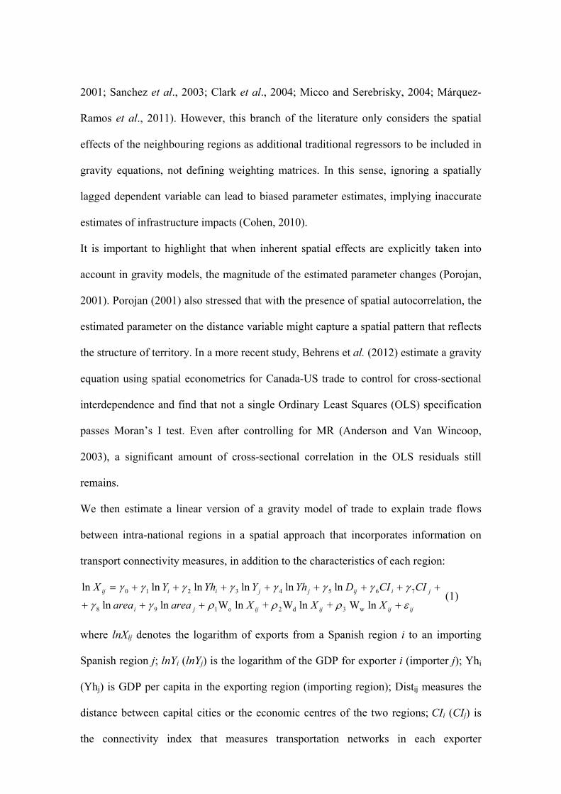
In a gravity framework that uses symmetrical spatial interaction data,4 we have to

amplify the weighting matrix and build an n2 *n2 matrix to take into account all trade

flows between all regions. For example, the model matrices might be defined as

, if W is n*n, then is n2 * n2. Note that in this type of model the spatial

effect is amplified because of the dimension of the flow model, as each region has a

relationship with the other regions.

2 This application does not contain any form of geographic connectivity as they use a similarity measure based on the relative size of regions.3 They construct a measure of transport connectivity to include in the weighting matrices.4 Recently, Márquez-Ramos (2014) uses a spatial approach with asymmetrical spatial interaction data (i.e. the number of origins is different from the number of destinations. Moreover, origins cannot also be destinations).

By using �“destination-centric ordering�”, we consider three types of indirect effects in

this paper: 1) , 2) and 3) . Where W matrix

represents an n by n spatial weight matrix based on a neighbour�’s criteria of

geographical first-order contiguity. Non-zero values for elements i and j denote that

zone i neighbours zone j, whereas zero values denote that zones i and j are not

neighbours. The elements on the diagonal are zero to prevent an observation from being

defined as being its own neighbour.

It is important to highlight that when working with autoregressive specifications, as is

the case with this paper, the structure of the model implies that the influence of the

�“neighbours of neighbours�” is taken into account. Consequently, with an autoregressive

type model in a territorially highly-disaggregated trade dataset, we are taking into

account �“second order�” neighbour relations that generate the abovementioned problem

of excessive contiguity.

2.2. A theoretically justified gravity approach with spatial lags

According to the traditional gravity model of trade (Anderson, 1979), the volume of

aggregate exports between pairs of regions and/or countries, depends on their income,

geographical distance and a series of dichotomous variables. Trade is expected to be

positively related to income and negatively related to distance. Gravity models applied

to the study of trade flows among countries normally include dichotomous variables

such as whether or not the trading partners share the same language or have a common

border, as well as variables for free trade agreements in order to assess the effects of

regional integration. Distance is also included in most empirical studies that employ

gravity equations as a proxy for transport costs.

The concept of transport connectivity has already been considered in gravity studies of

trade by means of analysing transport�–cost reducing measures (Limao and Venables,

2001; Sanchez et al., 2003; Clark et al., 2004; Micco and Serebrisky, 2004; Márquez-

Ramos et al., 2011). However, this branch of the literature only considers the spatial

effects of the neighbouring regions as additional traditional regressors to be included in

gravity equations, not defining weighting matrices. In this sense, ignoring a spatially

lagged dependent variable can lead to biased parameter estimates, implying inaccurate

estimates of infrastructure impacts (Cohen, 2010).

It is important to highlight that when inherent spatial effects are explicitly taken into

account in gravity models, the magnitude of the estimated parameter changes (Porojan,

2001). Porojan (2001) also stressed that with the presence of spatial autocorrelation, the

estimated parameter on the distance variable might capture a spatial pattern that reflects

the structure of territory. In a more recent study, Behrens et al. (2012) estimate a gravity

equation using spatial econometrics for Canada-US trade to control for cross-sectional

interdependence and find that not a single Ordinary Least Squares (OLS) specification

passes Moran�’s I test. Even after controlling for MR (Anderson and Van Wincoop,

2003), a significant amount of cross-sectional correlation in the OLS residuals still

remains.

We then estimate a linear version of a gravity model of trade to explain trade flows

between intra-national regions in a spatial approach that incorporates information on

transport connectivity measures, in addition to the characteristics of each region:

ijijijijji

jiijjjiiij

XXXareaareaCICIDYhYYhYX

ln W+lnW +ln Wlnlnlnlnlnlnlnln

w3d2o198

76543210 (1)

where lnXij denotes the logarithm of exports from a Spanish region i to an importing

Spanish region j; lnYi (lnYj) is the logarithm of the GDP for exporter i (importer j); Yhi

(Yhj) is GDP per capita in the exporting region (importing region); Distij measures the

distance between capital cities or the economic centres of the two regions; CIi (CIj) is

the connectivity index that measures transportation networks in each exporter

(importer), which has been calculated using information on the number of logistics

facilities and the number of square kilometres of logistics zones at the NUTS3 level

(Suárez-Burguet, 2012); following LeSage and Polasek (2008), we also include areai

(areaj) to control for the area of the origin and destination regions. The spatial lag vector

would be constructed by averaging flows from neighbours to the origin region

and parameter 1 would capture the magnitude of the impact of this type of

neighbouring observation on the dependent variable. The spatial lag vector

would be constructed by averaging flows from neighbours to the destination region and

parameter 2 would measure the impact and significance of flows from origin to all

neighbours of the destination region. The third spatial lag in the model is

constructed using an average of all neighbours to both the origin and destination

regions. Estimating parameters 1, 2 and 3 provides an inference of the relative

importance of the three types of spatial dependence between the origin and destination

regions. Then, 1, 2 and 3 are the spatial autocorrelation coefficients and the null

hypotheses test that 1=0; 2=0 and 3=0. Rejecting these null hypotheses implies that

trade flows from/in one region are directly affected by the importance of trade flows

from /in neighbouring regions. Finally, is a random disturbance.

We estimate two additional specifications derived from equation (1). First, we take into

account a remoteness factor in our gravity analysis by incorporating proxy variables and

also using spatial lags, in line with Márquez-Ramos (2014). Then, we estimate equation

(2):

ijijijijjij

ijiijjjiiij

XXXremremareaareaCICIDistYhYYhYX

ln WlnW +ln Wlnlnlnlnlnlnlnlnlnln

w3d2o111109

876543210

(2)

Where remi (remj) is the variable exporter (importer) remoteness based on equation 2a

(2b). That is, for a given origin-destination pair i and j, the degree of remoteness of

region i is defined as:

jw

ijji Y

DistYrem (2a)

where wY is the sum of the income of the importing regions of region i considered in

this study (total GDP in the Spanish peninsula). Similarly, the variable remoteness is

also calculated for the importer:

iw

ijij Y

DistYrem (2b)

In order to control MR factors, dummies for exporters and importers can be added to the

empirical model instead of remoteness variables. However, since income, surface and

transport connectivity variables are region specific, we estimate an additional version of

equation (1) that includes country dummies for importers ( j ) and for exporters ( i ),

and assumes that the effect of the transport connectivity variables is of equal magnitude

for both exporters and importers (i.e. CIij=CIi*CIj):

ijijijijijijjiij XXXCIDistX ln W+lnW +ln Wlnln w3d2o1210

(3)

We estimate equations 1, 2 and 3 using instrumental variables (IV) (Gibbons and

Overman, 2012) and, as the dependent variable is for year 2007, we use the (7-year)

lagged dependent variable to construct the spatial lags, namely trade flows in 2000.

Consequently, the excluded instruments are 2000,o ln W ijX , 2000,d ln W ijX and

2000,w ln W ijX . One way of validating the results is to observe whether they are robust

for the different specifications (i.e. equations 1, 2 and 3).

2.3. The spatial econometric modelling of OD flows

LeSage and Pace (2009) and Behrens et al. (2012) suggest using spatial econometrics to

control for MR. Therefore, our second methodology is the spatial econometric flow

model (LeSage and Pace, 2008). Its purpose is to explain variation in the magnitude of

flows between each OD pair and it is based on the type of spatial autoregressive models appearing in

equation (4):

ijijijijijddooij XXXDistXXX ln W+lnW +ln Wlnln w3d2o1

(4)

As in gravity models, X�’s matrix captures the characteristics of origin and destination

regions that could influence bilateral trade. Each variable produces an n2 by 1 vector

with the associated parameters in origin i, o, and destination j, d. The dependent

variable represents an n by n square matrix of interregional flows from each of the n

origin regions to each of the n destination regions, where each of the n columns of the

flow matrix represents a different destination and the n rows reflect origins.

Our focus is on extending gravity equations and then, we consider a number of

characteristics of the origin and destination regions. As per LeSage and Polasek (2008),

the explanatory variables used to construct the matrices Xo (origin) and Xd (destination)

are the (logged) area, the (logged) population, the (logged) GDP per capita and the

(logged) employment in each region. In keeping with the existing literature (LeSage and

Polasek, 2008; Alamá-Sabater et al., 2011 and 2013), we estimate the variant of

equation (4) using maximum likelihood.

In a preliminary analysis and in order to compare results obtained when the model is

estimated with and without spatial lags, we rely on the maximum likelihood method to

test for spatial dependence. As the null hypothesis of absence of spatial dependence is

rejected, the gravity model that includes the spatial lags appears to be a better

alternative. In addition, lower values are produced for the Akaike Information Criterion

(AIC) and Root Mean Squared Error (RMSE), indicating that the spatial model is

preferred. Therefore, the empirical illustration relies on regressions that include the

spatial lags.

3. Data and variables

We generate a dataset containing total commodity flows transported between 47 of the

Spanish provinces during the year 2007 (see Figure A.1, Appendix).5 As we are

considering the interregional trade in the peninsula and the effect of trade with

bordering regions, neither the Canary and Balearic Islands, nor Ceuta and Melilla are

included in the regressions.

Weighting matrices have been constructed using a geographical criterion and

introducing logistics characteristics. The geographical criterion controls for contiguity

across regions (contiguity model) and we also consider the presence of logistics

platforms (connectivity model), i.e. the regions adjacent to A (origin) or B (destination)

that also have logistics platforms. To proxy for the quality and level of logistics factors

between OD regions, a transport connectivity index is calculated as a simple average of

two dimension indices, the number and the size of the logistics platforms.

Figures 1 and 2 show the number of logistics platforms and the logistics surface area as

a percentage of the total logistics surface area in Spain (by province), respectively.

Madrid, Barcelona, Zaragoza and Cadiz have the largest relative surface area of

logistics platforms, mainly due to the presence of very large logistics platforms in these

regions (such as the Zaragoza Logistics Centre in Aragon, the Madrid Barajas centre in

the Madrid region and the Port of Algeciras in Andalusia). Provinces such as Valencia,

in the Valencian Community, and a number of provinces in Andalusia-Extremadura

5 The Spanish Statistical Institute has been the source of information for explanatory variables and, as for the dependent variable, the data refer to 2007. Interregional trade data has been supplied by C-Intereg (Llano et al., 2009 and 2010) for the Relog Project (Suárez-Burguet, 2012). Note that trade data is available for two years: 2007 and 2000.

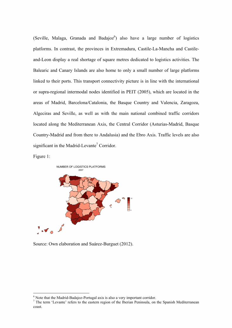
(Seville, Malaga, Granada and Badajoz6) also have a large number of logistics

platforms. In contrast, the provinces in Extremadura, Castile-La-Mancha and Castile-

and-Leon display a real shortage of square metres dedicated to logistics activities. The

Balearic and Canary Islands are also home to only a small number of large platforms

linked to their ports. This transport connectivity picture is in line with the international

or supra-regional intermodal nodes identified in PEIT (2005), which are located in the

areas of Madrid, Barcelona/Catalonia, the Basque Country and Valencia, Zaragoza,

Algeciras and Seville, as well as with the main national combined traffic corridors

located along the Mediterranean Axis, the Central Corridor (Asturias-Madrid, Basque

Country-Madrid and from there to Andalusia) and the Ebro Axis. Traffic levels are also

significant in the Madrid-Levante7 Corridor.

Figure 1:

19

0

2007

NUMBER OF LOGISTICS PLATFORMS

Source: Own elaboration and Suárez-Burguet (2012).

6 Note that the Madrid-Badajoz-Portugal axis is also a very important corridor.7 The term �‘Levante�’ refers to the eastern region of the Iberian Peninsula, on the Spanish Mediterranean coast.

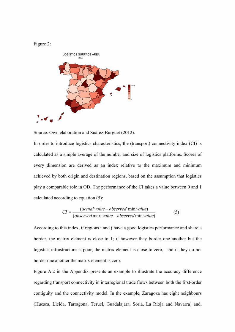
Figure 2:

17.48

0

2007

LOGISTICS SURFACE AREA


In order to introduce logistics characteristics, the (transport) connectivity index (CI) is

calculated as a simple average of the number and size of logistics platforms. Scores of

every dimension are derived as an index relative to the maximum and minimum

achieved by both origin and destination regions, based on the assumption that logistics

play a comparable role in OD. The performance of the CI takes a value between 0 and 1

calculated according to equation (5):

)minmax(

)min(valueobservedvalueobserved

valueobservedvalueactualCI (5)

According to this index, if regions i and j have a good logistics performance and share a

border, the matrix element is close to 1; if however they border one another but the

logistics infrastructure is poor, the matrix element is close to zero, and if they do not

border one another the matrix element is zero.

Figure A.2 in the Appendix presents an example to illustrate the accuracy difference

regarding transport connectivity in interregional trade flows between both the first-order

contiguity and the connectivity model. In the example, Zaragoza has eight neighbours

(Huesca, Lleida, Tarragona, Teruel, Guadalajara, Soria, La Rioja and Navarra) and,

whereas in the contiguity model the eight regions are assigned equal weights (the

geographical criteria are the same for all regions), in the connectivity model the

imposed filter weights the eight regions with the connectivity index defined above,

resulting in three regions being allocated the highest weightings (Tarragona,

Guadalajara and Navarra).

In order to explain the model and the dependent variable, we generate an n2 by 1 vector

by stacking the columns of the matrix. If we consider a model with four regions, the

flow matrix would appear as in Table 1. Columns show the dyad label (4 origin regions

x 4 destination regions = 16), identifier (ID) of the origin region and ID of the

destination region. Y denotes the dependent variable (exports)8 and Xs the explanatory

variables (for example, in the second methodology, area, population, GDP per capita

and employment, together with geographical distance). For simplicity, only four regions

(Seville, Zaragoza, Barcelona and Madrid) are considered in Table 1.

Table 1: Data organization

Dyad labels

Region origin ID origin

Region destination

ID destination

Origin explanation variables

Destination explanation variables

Distances

Y X1 X2 X3 X1 X2 X3 1 Seville 1 Seville 1 y11 a11 a12 a13 b11 b12 b13 d11 2 Zaragoza 2 Seville 1 y21 a21 a22 a23 b11 b12 b13 d21 3 Barcelona 3 Seville 1 y31 a31 a32 a33 b11 b12 b13 d31 4 Madrid 4 Seville 1 y41 a41 a42 a43 b11 b12 b13 d41 5 Seville 1 Zaragoza 2 y12 a11 a12 a13 b21 b22 b23 d12 6 Zaragoza 2 Zaragoza 2 y22 a21 a22 a23 b21 b22 b23 d22 7 Barcelona 3 Zaragoza 2 y32 a31 a32 a33 b21 b22 b23 d32 8 Madrid 4 Zaragoza 2 y42 a41 a42 a43 b21 b22 b23 d42 9 Seville 1 Barcelona 3 y13 a11 a12 a13 b31 b32 b33 d13 10 Zaragoza 2 Barcelona 3 y23 a21 a22 a23 b31 b32 b33 d23 11 Barcelona 3 Barcelona 3 y33 a31 a32 a33 b31 b32 b33 d33 12 Madrid 4 Barcelona 3 y43 a41 a42 a43 b31 b32 b33 d43 13 Seville 1 Madrid 4 y14 a11 a12 a13 b41 b42 b43 d14

8 Note that shipments made between regions within the customs territory of the European Union are no longer considered exports but rather intra-community supplies of goods and, more specifically, expeditions (or introductions, when it comes to goods receipts). Therefore, exports denote shipments from the origin to the destination Spanish region.

14 Zaragoza 2 Madrid 4 y24 a21 a22 a23 b41 b42 b43 d24 15 Barcelona 3 Madrid 4 y34 a31 a32 a33 b41 b42 b43 d34 16 Madrid 4 Madrid 4 y44 a41 a42 a43 b41 b42 b43 d44

In the empirical analysis we use the two methodologies described above. A first variant

of our models includes only first-order contiguity (contiguity-based model, with a

modified matrix Wm_contiguity), whereas our second variant of the model (transport

connectivity model, with a modified matrix Wm_connectivity) reflects transportation

networks in Spanish provinces by using the surface area and size of logistics platforms.

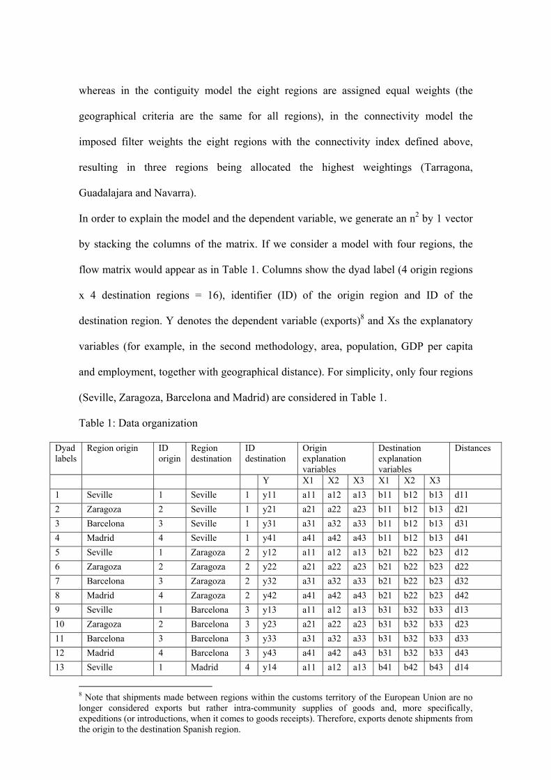
As a descriptive analysis, we present a map of Spain showing regions containing total

trade flows, as export-trade (Figure 3) and as import-trade (Figure 4).9 The areas where

the most important trade flows are concentrated are identified with darker colours (a

darker shade of red reflects higher levels of flow, while lighter shades of red indicate

lower levels). These maps represent total trade flows, so the analysis should be carried

out from a general point of view. According to our data, the Spanish regions with the

most outward and inward interregional trade flows are Barcelona, Madrid, Seville and

Valencia.10

Figure 3:

1.5e+08

720621

Total trade (tonnes) 2007

SPANISH PROVINCES (NUTS 3) BY EXPORT INTENSITY (OUTFLOWS)

Source: Own elaboration. 9 These maps are constructed by setting flows within regions to zero to emphasise interregional flows.10 Note that the maps on intensity of trade flows are measured in tonnes. As a result, they do not control for the value/volume relation of flows. Consequently, a number of regions could appear to be very important trading regions, although in reality they are not.

Figure 4:

1.5e+08

4.5e+06

Total trade (tonnes) 2007

SPANISH PROVINCES (NUTS 3) BY IMPORT INTENSITY (INFLOWS)

Source: Own elaboration.

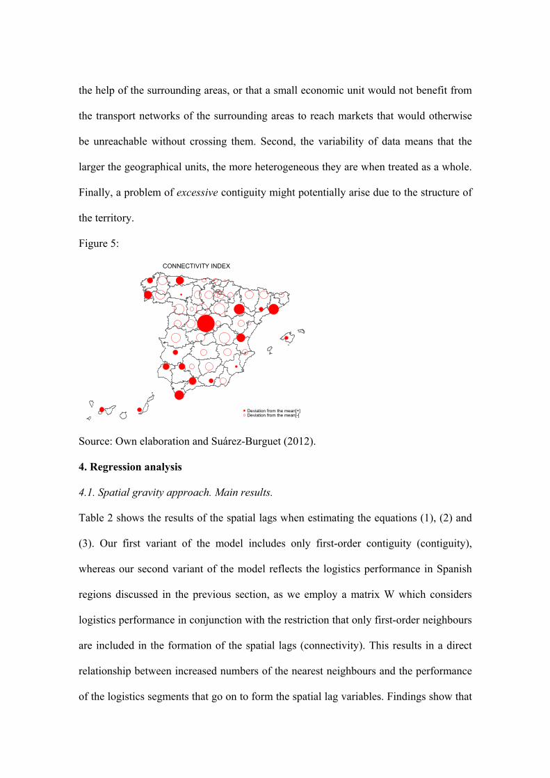
Figure 5 shows the map of the connectivity index derived from equation (5).11

Examining the maps in Figures 3 and 4 in conjunction with that of the logistics network

in Figure 5, there appears to be more flows in origin and destination regions in the

provinces where logistics networks are more extensive than in provinces with less

developed logistics networks. Therefore, in the case of Spain, a clear differentiation can

be made between provinces in terms of logistics performance. This descriptive test

emphasizes the need to explicitly incorporate such information into the spatial and

network dependence structure when analysing trade flows, as it might result in

substantial differences in the estimates and inferences. It can also be compared to

previous research that uses the spatial econometric flow model at the NUTS2 level in

Spain (Alamá-Sabater et al., 2011 and 2013). Although their results support the use of

an empirical framework where the spatial dependence of interregional trade flows is

introduced, they also provide evidence of the limited significance of spatial lags.12 It is

therefore expected that the higher the level of disaggregation of geographical data, the

greater the positive effect of the spatial lags. There are three main reasons for this: First,

it seems unlikely that a small spatial economic unit could produce many goods without

11 The regions containing the highest values are in dark red.12 The Moran's I statistic is used to analyse the existence of spatial autocorrelation.

the help of the surrounding areas, or that a small economic unit would not benefit from

the transport networks of the surrounding areas to reach markets that would otherwise

be unreachable without crossing them. Second, the variability of data means that the

larger the geographical units, the more heterogeneous they are when treated as a whole.

Finally, a problem of excessive contiguity might potentially arise due to the structure of

the territory.

Figure 5:

Deviation from the mean[+]Deviation from the mean[-]

CONNECTIVITY INDEX


4. Regression analysis

4.1. Spatial gravity approach. Main results.

Table 2 shows the results of the spatial lags when estimating the equations (1), (2) and

(3). Our first variant of the model includes only first-order contiguity (contiguity),

whereas our second variant of the model reflects the logistics performance in Spanish

regions discussed in the previous section, as we employ a matrix W which considers

logistics performance in conjunction with the restriction that only first-order neighbours

are included in the formation of the spatial lags (connectivity). This results in a direct

relationship between increased numbers of the nearest neighbours and the performance

of the logistics segments that go on to form the spatial lag variables. Findings show that

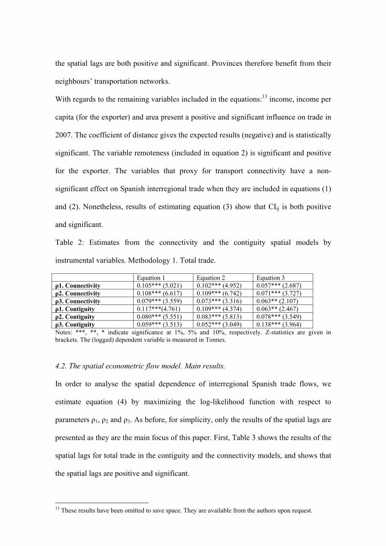
the spatial lags are both positive and significant. Provinces therefore benefit from their

neighbours�’ transportation networks.

With regards to the remaining variables included in the equations:13 income, income per

capita (for the exporter) and area present a positive and significant influence on trade in

2007. The coefficient of distance gives the expected results (negative) and is statistically

significant. The variable remoteness (included in equation 2) is significant and positive

for the exporter. The variables that proxy for transport connectivity have a non-

significant effect on Spanish interregional trade when they are included in equations (1)

and (2). Nonetheless, results of estimating equation (3) show that CIij is both positive

and significant.

Table 2: Estimates from the connectivity and the contiguity spatial models by

instrumental variables. Methodology 1. Total trade.

Equation 1 Equation 2 Equation 3 1. Connectivity 0.105*** (5.021) 0.102*** (4.952) 0.057*** (2.687) 2. Connectivity 0.108*** (6.617) 0.109*** (6.742) 0.071*** (3.727) 3. Connectivity 0.079*** (3.559) 0.073*** (3.316) 0.063** (2.107) 1. Contiguity 0.117***(4.761) 0.109*** (4.374) 0.063** (2.467) 2. Contiguity 0.080*** (5.551) 0.083*** (5.813) 0.078*** (3.549) 3. Contiguity 0.059*** (3.513) 0.052*** (3.049) 0.138*** (3.964)

Notes: ***, **, * indicate significance at 1%, 5% and 10%, respectively. Z-statistics are given in brackets. The (logged) dependent variable is measured in Tonnes.

4.2. The spatial econometric flow model. Main results.

In order to analyse the spatial dependence of interregional Spanish trade flows, we

estimate equation (4) by maximizing the log-likelihood function with respect to

parameters 1, 2 and 3. As before, for simplicity, only the results of the spatial lags are

presented as they are the main focus of this paper. First, Table 3 shows the results of the

spatial lags for total trade in the contiguity and the connectivity models, and shows that

the spatial lags are positive and significant.

13 These results have been omitted to save space. They are available from the authors upon request.

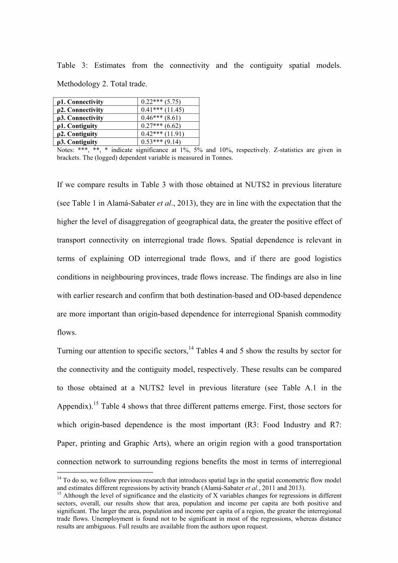
Table 3: Estimates from the connectivity and the contiguity spatial models.

Methodology 2. Total trade.

1. Connectivity 0.22*** (5.75) 2. Connectivity 0.41*** (11.45) 3. Connectivity 0.46*** (8.61) 1. Contiguity 0.27*** (6.62) 2. Contiguity 0.42*** (11.91) 3. Contiguity 0.53*** (9.14)


If we compare results in Table 3 with those obtained at NUTS2 in previous literature

(see Table 1 in Alamá-Sabater et al., 2013), they are in line with the expectation that the

higher the level of disaggregation of geographical data, the greater the positive effect of

transport connectivity on interregional trade flows. Spatial dependence is relevant in

terms of explaining OD interregional trade flows, and if there are good logistics

conditions in neighbouring provinces, trade flows increase. The findings are also in line

with earlier research and confirm that both destination-based and OD-based dependence

are more important than origin-based dependence for interregional Spanish commodity

flows.

Turning our attention to specific sectors,14 Tables 4 and 5 show the results by sector for

the connectivity and the contiguity model, respectively. These results can be compared

to those obtained at a NUTS2 level in previous literature (see Table A.1 in the

Appendix).15 Table 4 shows that three different patterns emerge. First, those sectors for

which origin-based dependence is the most important (R3: Food Industry and R7:

Paper, printing and Graphic Arts), where an origin region with a good transportation

connection network to surrounding regions benefits the most in terms of interregional 14 To do so, we follow previous research that introduces spatial lags in the spatial econometric flow model and estimates different regressions by activity branch (Alamá-Sabater et al., 2011 and 2013).15 Although the level of significance and the elasticity of X variables changes for regressions in different sectors, overall, our results show that area, population and income per capita are both positive and significant. The larger the area, population and income per capita of a region, the greater the interregional trade flows. Unemployment is found not to be significant in most of the regressions, whereas distance results are ambiguous. Full results are available from the authors upon request.

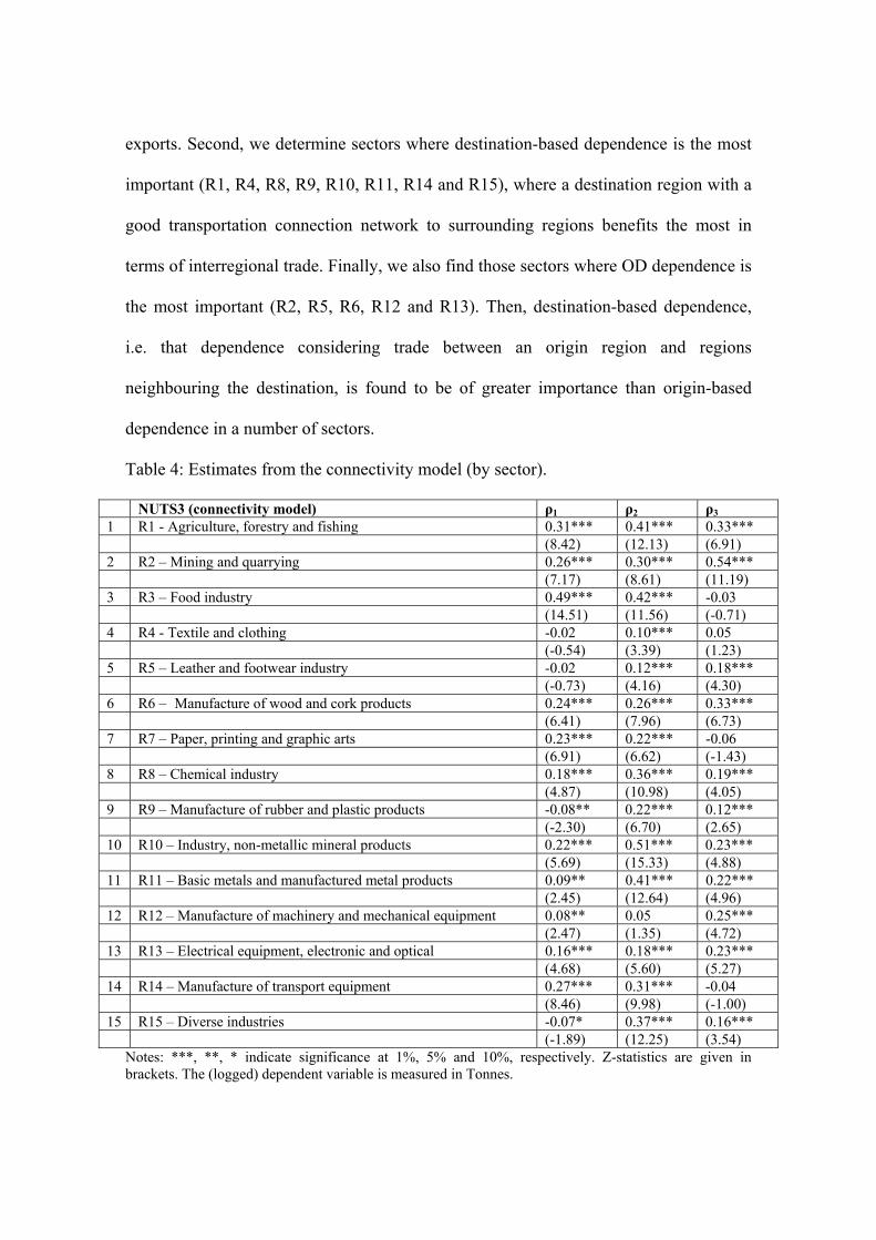
exports. Second, we determine sectors where destination-based dependence is the most

important (R1, R4, R8, R9, R10, R11, R14 and R15), where a destination region with a

good transportation connection network to surrounding regions benefits the most in

terms of interregional trade. Finally, we also find those sectors where OD dependence is

the most important (R2, R5, R6, R12 and R13). Then, destination-based dependence,

i.e. that dependence considering trade between an origin region and regions

neighbouring the destination, is found to be of greater importance than origin-based

dependence in a number of sectors.

Table 4: Estimates from the connectivity model (by sector).


NUTS3 (connectivity model) 1 2 3

1 R1 - Agriculture, forestry and fishing 0.31*** 0.41*** 0.33*** (8.42) (12.13) (6.91) 2 R2 �– Mining and quarrying 0.26*** 0.30*** 0.54*** (7.17) (8.61) (11.19) 3 R3 �– Food industry 0.49*** 0.42*** -0.03 (14.51) (11.56) (-0.71) 4 R4 - Textile and clothing -0.02 0.10*** 0.05 (-0.54) (3.39) (1.23) 5 R5 �– Leather and footwear industry -0.02 0.12*** 0.18*** (-0.73) (4.16) (4.30) 6 R6 �– Manufacture of wood and cork products 0.24*** 0.26*** 0.33*** (6.41) (7.96) (6.73) 7 R7 �– Paper, printing and graphic arts 0.23*** 0.22*** -0.06 (6.91) (6.62) (-1.43) 8 R8 �– Chemical industry 0.18*** 0.36*** 0.19*** (4.87) (10.98) (4.05) 9 R9 �– Manufacture of rubber and plastic products -0.08** 0.22*** 0.12*** (-2.30) (6.70) (2.65) 10 R10 �– Industry, non-metallic mineral products 0.22*** 0.51*** 0.23*** (5.69) (15.33) (4.88) 11 R11 �– Basic metals and manufactured metal products 0.09** 0.41*** 0.22*** (2.45) (12.64) (4.96) 12 R12 �– Manufacture of machinery and mechanical equipment 0.08** 0.05 0.25*** (2.47) (1.35) (4.72) 13 R13 �– Electrical equipment, electronic and optical 0.16*** 0.18*** 0.23*** (4.68) (5.60) (5.27) 14 R14 �– Manufacture of transport equipment 0.27*** 0.31*** -0.04 (8.46) (9.98) (-1.00) 15 R15 �– Diverse industries -0.07* 0.37*** 0.16*** (-1.89) (12.25) (3.54)

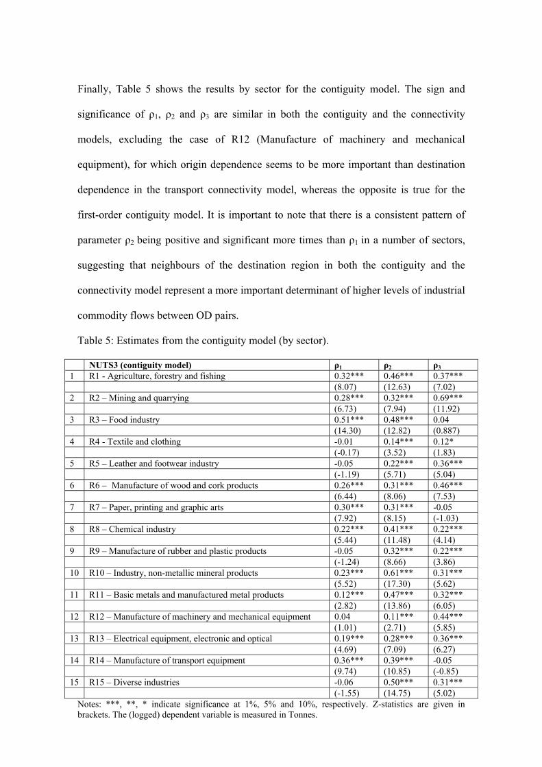
Finally, Table 5 shows the results by sector for the contiguity model. The sign and

significance of 1, 2 and 3 are similar in both the contiguity and the connectivity

models, excluding the case of R12 (Manufacture of machinery and mechanical

equipment), for which origin dependence seems to be more important than destination

dependence in the transport connectivity model, whereas the opposite is true for the

first-order contiguity model. It is important to note that there is a consistent pattern of

parameter 2 being positive and significant more times than 1 in a number of sectors,

suggesting that neighbours of the destination region in both the contiguity and the

connectivity model represent a more important determinant of higher levels of industrial

commodity flows between OD pairs.

Table 5: Estimates from the contiguity model (by sector).


NUTS3 (contiguity model) 1 2 3

1 R1 - Agriculture, forestry and fishing 0.32*** 0.46*** 0.37*** (8.07) (12.63) (7.02) 2 R2 �– Mining and quarrying 0.28*** 0.32*** 0.69*** (6.73) (7.94) (11.92) 3 R3 �– Food industry 0.51*** 0.48*** 0.04 (14.30) (12.82) (0.887) 4 R4 - Textile and clothing -0.01 0.14*** 0.12* (-0.17) (3.52) (1.83) 5 R5 �– Leather and footwear industry -0.05 0.22*** 0.36*** (-1.19) (5.71) (5.04) 6 R6 �– Manufacture of wood and cork products 0.26*** 0.31*** 0.46*** (6.44) (8.06) (7.53) 7 R7 �– Paper, printing and graphic arts 0.30*** 0.31*** -0.05 (7.92) (8.15) (-1.03) 8 R8 �– Chemical industry 0.22*** 0.41*** 0.22*** (5.44) (11.48) (4.14) 9 R9 �– Manufacture of rubber and plastic products -0.05 0.32*** 0.22*** (-1.24) (8.66) (3.86) 10 R10 �– Industry, non-metallic mineral products 0.23*** 0.61*** 0.31*** (5.52) (17.30) (5.62) 11 R11 �– Basic metals and manufactured metal products 0.12*** 0.47*** 0.32*** (2.82) (13.86) (6.05) 12 R12 �– Manufacture of machinery and mechanical equipment 0.04 0.11*** 0.44*** (1.01) (2.71) (5.85) 13 R13 �– Electrical equipment, electronic and optical 0.19*** 0.28*** 0.36*** (4.69) (7.09) (6.27) 14 R14 �– Manufacture of transport equipment 0.36*** 0.39*** -0.05 (9.74) (10.85) (-0.85) 15 R15 �– Diverse industries -0.06 0.50*** 0.31*** (-1.55) (14.75) (5.02)

5. Conclusions

This paper analyses the role of transport connectivity in interregional trade flows using

a spatial approach by using highly-disaggregated regional trade data at a provincial level

in Spain. In order to do so, we use a gravity framework and take into account

multilateral resistance in a two-methodology comparison. In order to test whether

incorporating transport connectivity information into the spatial structure of the model

results in substantial differences in the estimates, we have defined different types of

neighbour relations. In particular, two different variants of the model were estimated,

based on first-order contiguity and transport connectivity criteria in order to construct

the weighting matrices.

We find evidence that transport connectivity has a bearing on interregional trade.

Moreover, we show that forces leading to flows from an origin province to a destination

province would create similar flows to neighbouring destinations. Regions therefore

benefit from their neighbours�’ transport connectivity. These results not only provide

evidence about the role of the location of logistics platforms in satisfying the existing

demand for transport structures, but also as to the benefit of introducing spatial

dependence in gravity models of trade when analysing interregional trade flows, as

ignoring spatial lags might lead to biased estimation of the parameters.

References

- Alamá-Sabater, L., Márquez-Ramos, L. and Suárez-Burguet, C. (2011) La

relación entre el comercio interregional y la conectividad del transporte en

España. Un análisis de dependencia espacial, Revista de Economía y Estadística,

XLIX (1), 7-32.

- Alamá-Sabater, L., Márquez-Ramos, L. and Suárez-Burguet, C. (2013) Trade

and transport connectivity: a spatial approach, Applied Economics, 45, 2563-

2566.

- Anderson, J. E. (1979) A theoretical foundation for the gravity equation,

American Economic Review, 69, 106-116.

- Anderson, J. E. and Van Wincoop, E. (2003) Gravity with gravitas: A solution to

the border puzzle, American Economic Review, 93, 170-192.

- Anselin, L. (1988) Spatial Econometrics: Methods and Models, Dordrecht:

Kluwer Academic Publishers.

- Behrens, K., Ertur, C., and Koch, W. (2012) 'Dual'gravity: Using spatial

econometrics to control for multilateral resistance, Journal of Applied

Econometrics, 27, 773�–794.

- Clark, X., Dollar, D. and A. Micco (2004) Port efficiency, maritime transport

costs, and bilateral trade, Journal of Development Economics, 75, 417�–450.

- Cohen, J. P. (2010) The broader effects of transportation infrastructure: Spatial

econometrics and productivity approaches, Transportation Research Part E:

Logistics and Transportation Review, 46, 317-326.

- Corrado, L. and Fingleton, B. (2012) Where Is The Economics In Spatial

Econometrics?, Journal of Regional Science, 52, 210-239.

- De la Mata, T. and Llano-Verduras, C. (2012) Spatial pattern and domestic

tourism: An econometric analysis using inter-regional monetary flows by type of

journey, Papers in Regional Science, 91, 437�–470.

- Gibbons, S. and Overman, H. G. (2012) Mostly Pointless Spatial Econometrics?,

Journal of Regional Science, 52, 172-191.

- Hierro, M. and Maza, A. (2010) Per capita income convergence and internal

migration in Spain: Are foreign born migrants playing an important role?,

Papers in Regional Science, 89, 89-107.

- LeSage J.P. and Pace R.K. (2004) Introduction to Spatial and Spatiotemporal in

Spatial and Spatiotemporal Econometrics. Published by James P. LeSage and R.

Kelley Pace, 18, Oxford: Elsevier Ltd.

- LeSage J.P. and Pace R.K. (2008) Spatial econometric modelling of origin-

destination flows, Journal of Regional Science, 5, 941-967.

- LeSage, J. P. and Llano, C. (2013) A spatial interaction model with spatially

structured origin and destination effects, Journal of Geographical Systems, 15,

265-289.

- LeSage, J. P. and Thomas-Agnan, C. (2014) Interpreting spatial econometrics

origin-destination flow models, Journal of Regional Science,

DOI: 10.1111/jors.12114

- LeSage, J. P., and Polasek W. (2008) Incorporating transportation network

structure in spatial econometric models of commodity flows. Spatial Economic

Analysis, 3, 225-245.

- Limao, N, and Venables, AJ (2001) Infrastructure, Geographical Disadvantage

and Transport Costs, World Bank Economic Review, 15, 451-479.

- Llano C., Esteban, A., Pérez, J., Pulido, A. (2009) Metodología de estimación de

la base de datos C-intereg sobre el comercio interregional de bienes en España

(1995-05), Ekonomiaz, 69, 244-270.

- Llano, C., Esteban, A., Pérez, J., Pulido, A. (2010) Opening the Interregional

Trade Black Box: The C-intereg Database for the Spanish Economy (1995-

2005), International Regional Science Review, 33, 302-337.

- Márquez-Ramos, L. (2014) Port Facilities, Regional Spillovers and Exports:

Empirical Evidence from Spain, Papers in Regional Science, DOI:

10.1111/pirs.12127

- Márquez-Ramos, L., Martínez-Zarzoso, I., Pérez-García, E. and Wilmsmeier, G.

(2011) Special Issue on Latin-American Research, Maritime Networks, Services

Structure and Maritime Trade. Networks and Spatial Economics, 11, 555-76.

- Micco, A. and Serebrisky, T. (2004) Infrastructure, competition regimes, and air

transport costs: Cross-country evidence, Policy Research Working Paper Series

3355, The World Bank.

- PEIT (2005) Plan Estratégico de Infraestructuras y Transporte - Strategic

Infrastructures and Transport Plan (2005-2020), Centro de Publicaciones

Secretaría General Técnica Ministerio de Fomento, Madrid.

- Porojan, A. (2001) Trade flows and spatial effects: the gravity model revisited,

Open Economies Review, 12, 265-280.

- Rodrigue, J-P., Comtois, C. and Slack, B. (2013) The geography of transport

systems, New York: Routledge. 3rd Edition.

- Sanchez, R. J., Hoffmann, J., Micco, A., Pizzolitto, G.M., Sgut, M. and

Wilmsmeier, G. (2003) Port Efficiency and International Trade: Port Efficiency

as a Determinant of Maritime Transport Costs, Maritime Economics &

Logistics, 5, 199�–218.

- Suárez-Burguet C. (dir.) (2012) Definition of a Spanish Logistics Platforms

Network, RELOG, Technical Report, mimeo, Ministry of Transport, Madrid.

APPENDIX

Figure A.1. Provinces in Spain (NUTS3).

Note: The provinces in the same colour belong to the same Autonomous Community (NUTS2). Source: Hierro and Maza (2010).

Figure A.2. First-order contiguity versus transport connectivity model.

Source: Own elaboration

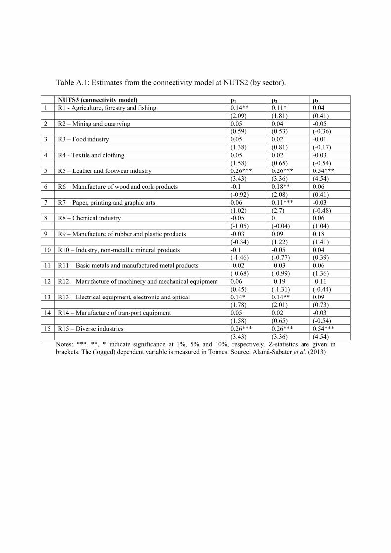
Table A.1: Estimates from the connectivity model at NUTS2 (by sector).

NUTS3 (connectivity model) 1 2 3

1 R1 - Agriculture, forestry and fishing 0.14** 0.11* 0.04 (2.09) (1.81) (0.41) 2 R2 �– Mining and quarrying 0.05 0.04 -0.05 (0.59) (0.53) (-0.36) 3 R3 �– Food industry 0.05 0.02 -0.01 (1.38) (0.81) (-0.17) 4 R4 - Textile and clothing 0.05 0.02 -0.03 (1.58) (0.65) (-0.54) 5 R5 �– Leather and footwear industry 0.26*** 0.26*** 0.54*** (3.43) (3.36) (4.54) 6 R6 �– Manufacture of wood and cork products -0.1 0.18** 0.06 (-0.92) (2.08) (0.41) 7 R7 �– Paper, printing and graphic arts 0.06 0.11*** -0.03 (1.02) (2.7) (-0.48) 8 R8 �– Chemical industry -0.05 0 0.06 (-1.05) (-0.04) (1.04) 9 R9 �– Manufacture of rubber and plastic products -0.03 0.09 0.18 (-0.34) (1.22) (1.41) 10 R10 �– Industry, non-metallic mineral products -0.1 -0.05 0.04 (-1.46) (-0.77) (0.39) 11 R11 �– Basic metals and manufactured metal products -0.02 -0.03 0.06 (-0.68) (-0.99) (1.36) 12 R12 �– Manufacture of machinery and mechanical equipment 0.06 -0.19 -0.11 (0.45) (-1.31) (-0.44) 13 R13 �– Electrical equipment, electronic and optical 0.14* 0.14** 0.09 (1.78) (2.01) (0.73) 14 R14 �– Manufacture of transport equipment 0.05 0.02 -0.03 (1.58) (0.65) (-0.54) 15 R15 �– Diverse industries 0.26*** 0.26*** 0.54*** (3.43) (3.36) (4.54)

Notes: ***, **, * indicate significance at 1%, 5% and 10%, respectively. Z-statistics are given in brackets. The (logged) dependent variable is measured in Tonnes. Source: Alamá-Sabater et al. (2013)

a two-methodology comparison study of a spatial gravity

Documents