A TWO-PHASE GRADIENT METHOD FOR QUADRATICPROGRAMMING PROBLEMS WITH A SINGLE LINEAR

CONSTRAINT AND BOUNDS ON THE VARIABLES∗

DANIELA DI SERAFINO† , GERARDO TORALDO‡ , MARCO VIOLA§ , AND JESSE

BARLOW¶

FINAL VERSION – May 25, 2018

Abstract. We propose a gradient-based method for quadratic programming problems with asingle linear constraint and bounds on the variables. Inspired by the GPCG algorithm for bound-constrained convex quadratic programming [J.J. More and G. Toraldo, SIAM J. Optim. 1, 1991],our approach alternates between two phases until convergence: an identification phase, which per-forms gradient projection iterations until either a candidate active set is identified or no reasonableprogress is made, and an unconstrained minimization phase, which reduces the objective function ina suitable space defined by the identification phase, by applying either the conjugate gradient methodor a recently proposed spectral gradient method. However, the algorithm differs from GPCG notonly because it deals with a more general class of problems, but mainly for the way it stops theminimization phase. This is based on a comparison between a measure of optimality in the reducedspace and a measure of bindingness of the variables that are on the bounds, defined by extending theconcept of proportional iterate, which was proposed by some authors for box-constrained problems.If the objective function is bounded, the algorithm converges to a stationary point thanks to a suit-able application of the gradient projection method in the identification phase. For strictly convexproblems, the algorithm converges to the optimal solution in a finite number of steps even in case ofdegeneracy. Extensive numerical experiments show the effectiveness of the proposed approach.

Key words. Quadratic programming, bound and single linear constraints, gradient projection,proportionality.

AMS subject classifications. 65K05, 90C20.

1. Introduction. We are concerned with the solution of Quadratic Program-ming problems with a Single Linear constraint and lower and upper Bounds on thevariables (SLBQPs):

min f(x) :=1

2xT H x− cTx,

s.t. qTx = b, l ≤ x ≤ u,(1.1)

where H∈ Rn×n is symmetric, c,q ∈ Rn, b ∈ R, l ∈R ∪ −∞n, u ∈R ∪ +∞n,and, without loss of generality, li < ui for all i. In general, we do not assume thatthe problem is strictly convex. SLBQPs arise in many applications, such as supportvector machine training [36], portfolio selection [33], multicommodity network flowand logistics [29], and statistics estimate from a target distribution [1]. Therefore,designing efficient methods for the solution of (1.1) has both a theoretical and apractical interest.

∗This work was partially supported by Gruppo Nazionale per il Calcolo Scientifico - IstitutoNazionale di Alta Matematica (GNCS-INdAM).†Dipartimento di Matematica e Fisica, Universita degli Studi della Campania L. Vanvitelli, viale

A. Lincoln 5, 81100 Caserta, Italy, daniela.diserafino@unicampania.it.‡Dipartimento di Matematica e Applicazioni R. Caccioppoli, Universita degli Studi di Napoli

Federico II, via Cintia, 80126 Napoli, Italy, toraldo@unina.it.§Dipartimento di Ingegneria Informatica Automatica e Gestionale A. Ruberti, Sapienza - Univer-

sita di Roma, via Ariosto 25, 00185 Roma, Italy, marco.viola@uniroma1.it.¶Department of Computer Science and Engineering, Pennsylvania State University, 343G IST

Building, University Park, PA 16802-6822, USA, barlow@cse.psu.edu.

1

Gradient Projection (GP) methods are widely used to solve large-scale SLBQPproblems, thanks to the availability of low-cost projection algorithms onto the feasibleset of (1.1) (see, e.g, [8, 12, 9]). In particular, Spectral Projected Gradient methods [4],other GP methods exploiting variants of Barzilai-Borwein (BB) steps [35, 12], andmore recent Scaled Gradient Projection methods [6] have proved their effectiveness inseveral applications.

Bound-constrained Quadratic Programming problems (BQPs) can be regarded asa special case of SLBQPs, where the theory or the implementation can be simplified.This has favoured the development of more specialized gradient-based methods, builtupon the idea of combining steps aimed at identifying the variables that are activeat a solution (or at a stationary point) with unconstrained minimizations in reducedspaces defined by fixing the variables that are estimated active [31, 24, 32, 25, 3, 20,22, 27, 21, 28]. Thanks to the identification properties of the GP method [7] and toits capability of adding/removing multiple variables to/from the active set in a singleiteration, GP steps are a natural choice to determine the active variables. A well-known method based on this approach is GPCG [32], developed for strictly convexBQPs. It alternates between two phases: an identification phase, which performsGP iterations until a suitable face of the feasible set is identified or no reasonableprogress toward the solution is achieved, and a minimization phase, which uses theConjugate Gradient (CG) method to find an approximate minimizer of the objectivefunction in the reduced space resulting from the identification phase. We note that theglobal convergence of the GPCG method relies on the global convergence of GP withsteplengths satisfying a suitable sufficient decrease condition [7]. Furthermore, GPCGhas finite convergence under a dual nondegeracy assumption, thanks to the ability ofthe GP method to identify the active constraints in a finite number of iterations [7],and to the finite termination of the CG method. Finally, the identification propertyalso holds for nonquadratic objective functions and polyhedral constraints, and thusthe algorithmic framework described so far can be extended to more general problems.

Here we propose a two-phase GP method for SLBQPs, called Proportionality-based 2-phase Gradient Projection (P2GP) method, inspired by the GPCG algorithm.Besides targeting problems more general than strictly convex BQPs, the new methoddiffers from GPCG because it follows a different approach in deciding when to ter-minate optimization in the reduced space. Whereas GPCG uses a heuristics basedon the bindingness of the active variables, P2GP relies on the comparison betweena measure of optimality within the reduced space and a measure of bindingness ofthe variables that are on the bounds. This approach exploits the concept of propor-tional iterate, henceforth also refereed to as proportionality. This concept, presentedby Dostal for strictly convex BQPs [20], is based on the splitting of the optimalityconditions between free and chopped gradients, firstly introduced by Friedlander andMartınez in [24]. To this end, we generalize the definition of free and chopped gradi-ents to problem (1.1). As in GPCG, and unlike other algorithms for BQPs sharing acommon ground (e.g., [20, 21, 22, 30]), the task of adjusting the active set is left onlyto the GP steps; thus, for strictly convex BQPs our algorithm differs from GPCG inthe criterion used to stop minimization of the reduced problem. This change makes asignificant difference in the effectiveness of the algorithm as our numerical experimentsshow. In addition, the application of the proportionality concept allows to state fi-nite convergence for strictly convex problems also for dual-degenerate solutions. Moregenerally, if the objective function is bounded, the algorithm converges to a stationarypoint as a result of suitable application of the GP method in the identification phase.

2

About the GP iterations, we note that the identification property holds providedthat a sufficient decrease condition holds, and therefore the choice of the Cauchystepsize as initial trial value in the projected gradient steps [31, 32] can be replacedby rules used by new spectral gradient methods. Inspired by encouraging resultsreported for BQPs in [11] and by further studies on steplength selection in gradientmethods [17, 18], we consider a monotone version of the Projected BB method whichuses the ABBmin steplength introduced in [23].

In the minimization phase, we use the CG method, and, in the strictly convexcase, we also use the SDC method proposed in [14]. This provides a way to extendSDC to the costrained case, with the goal of exploiting its smoothing and regularizingeffect observed on certain unconstrained ill-posed inverse problems [15]. Of course,the CG solver is still the reference choice in general, especially because it is able todeal with nonconvexity through directions of negative curvature (as done, e.g., in[30]), whereas handling negative curvatures with spectral gradient methods may be anon-trivial task (see, e.g., [10] and the references therein).

This article is organized as follows. In Section 2, we recall stationarity resultsfor problem (1.1). In Section 3, we define free and chopped gradients for SLBQPsand show how they can be used to extend the concept of proportionality to this classof problems. In Section 4, we describe the P2GP method and state its convergenceproperties. We discuss the results of extensive numerical experiments in Section 5,showing the effectiveness of our approach. We draw some conclusions in Section 6.

1.1. Notation. Throughout this paper scalars are denoted by lightface Romanfonts, e.g., a ∈ R, vectors by boldface Roman fonts, e.g., v ∈ Rn, and matrices byitalicized lightface capital fonts, e.g., M ∈ Rn×n. The vectors of the standard basisof Rn are indicated as e1, . . . , en. Given R, C ⊆ 1, . . . , n, we set

vR := (vi)i∈R, MRC := (mij)i∈R,j∈C ,

where vi is the ith entry of v and mij the (i, j)th entry of M . For any vector v, v⊥is the space orthogonal to v. For any symmetric matrix M , we use κ(M), ζmin(M)and ζmax(M) to indicate the condition number, and the minimum and maximumeigenvalue of M , respectively. Norms ‖ · ‖ are `2, unless otherwise stated.

The feasible set, Ω, of problem (1.1) is given by

Ω :=x ∈ Rn : qTx = b ∧ l ≤ x ≤ u

.

For any x ∈ Ω, we define the following index sets:

Al(x) := i : xi = li, Au(x) := i : xi = ui,A(x) := Al(x) ∪ Au(x), F(x) := 1, . . . , n \ A(x).

A(x) and F(x) are called the active and free sets at x, respectively. Given x,y ∈ Ω,by writing A(x) ⊆ A(y) we mean that

Al(x) ⊆ Al(y), Au(x) ⊆ Au(y)

both hold. For any x ∈ Ω, we also set

Ω(x) :=v ∈ Rn : qTv = b ∧ vi = xi ∀ i ∈ A(x)

, (1.2)

Ω0(x) :=v ∈ Rn : qTv = 0 ∧ vi = 0 ∀ i ∈ A(x)

. (1.3)

3

Note that Ω(x) is the affine closure of the face determined by the active set at x.We use superscripts to denote the elements of a sequence, e.g.,

xk

; furthermore,in order to simplify the notation, for any xk and x∗ we also define

fk := f(xk), ∇fk := ∇f(xk), Ak := A(xk), Fk := F(xk),

f∗ := f(x∗), ∇f∗ := ∇f(x∗), A∗ := A(x∗), F∗ := F(x∗).

Finally, for any finite set T , we denote by |T | its cardinality.

2. Stationarity results for SLBQPs. We recall that x∗ ∈ Ω is a stationarypoint for problem (1.1) if and only if there exist Lagrange multipliers ρ∗, λ∗i ∈ R, withi ∈ A∗, such that

∇f∗ =∑i∈A∗

λ∗i ei + ρ∗q, λ∗i ≥ 0 if i ∈ A∗l , λ∗i ≤ 0 if i ∈ A∗u, (2.1)

or, equivalently,∇f∗F∗ − ρ∗qF∗ = 0, (2.2)

λ∗i = ∇f∗i − ρ∗qi ≥ 0 if i ∈ A∗l , λ∗i = ∇f∗i − ρ∗qi ≤ 0 if i ∈ A∗u. (2.3)

If qF∗ 6= 0, by taking the scalar product of (2.2) with qF∗ , we obtain

ρ∗ =qTF∗ ∇f∗F∗qTF∗ qF∗

(with a little abuse of notation we include F∗ = ∅ in the case qF∗ = 0). Then, bydefining for all x ∈ Ω

ρ(x) :=

0 if qF= 0,

qTF ∇fF (x)

qTF qFotherwise,

(2.4)

where F = F(x), andh(x) := ∇f(x)− ρ(x)q, (2.5)

conditions (2.2)-(2.3) can be expressed as

h∗i = 0 if i ∈ F∗, h∗i ≥ 0 if i ∈ A∗l , h∗i ≤ 0 if i ∈ A∗u. (2.6)

This suggests the following definition.

Definition 2.1 (Binding set). For any x ∈ Ω, the binding set at x is defined as

B(x) := i : (i ∈ Al(x) ∧ hi(x) ≥ 0) ∨ (i ∈ Au(x) ∧ hi(x) ≤ 0) . (2.7)

We note that, for the BQP case, (2.7) corresponds to the standard definition of bindingset where h(x) is replaced by ∇f(x).

We can also provide an estimate of the Lagrange multipliers based on (2.5), asstated by the following theorem.

Theorem 2.2. Assume thatxk

is a sequence in Ω that converges to a nonde-generate stationary point x∗, and A(xk) = A(x∗) for all k sufficiently large. Then

limk→∞

ρ(xk) = ρ∗ and limk→∞

λi(xk) = λ∗i ∀i ∈ A∗, (2.8)

4

where λi(x) is defined as follows:

λi(x) :=

max0, hi(x) if i ∈ Al(x),min0, hi(x) if i ∈ Au(x),

0 if i ∈ F(x).

Proof. The result is a straightforward consequence of the continuity of ∇f .

Remark 2.1. Theorem 2.2 can be rephrased by saying that(ρ(x), λ(x)T

)T,

where λ(x) = (λi(x))i∈A(x), is a consistent Lagrange multiplier estimate for (1.1),according to the definition in [7, p. 107].

Another way to express stationarity for problem (2.1) is by using the projectedgradient of f at a point x ∈ Ω, defined by Calamai and More [7] as

∇Ωf(x) := argmin ‖v +∇f(x)‖ s.t. v ∈ TΩ(x) , (2.9)where

TΩ(x) =v ∈ Rn : qTv = 0 ∧ vi ≥ 0 ∀ i ∈ Al(x) ∧ vi ≤ 0 ∀ i ∈ Au(x)

is the tangent cone to Ω at x, i.e., the closure of the cone of all feasible directions at x.It is well known that x∗ ∈ Ω is a stationary point for (1.1) if and only if ∇Ωf(x∗) = 0,which is equivalent to

−∇f(x∗) ∈ TΩ(x),

where TΩ(x) =w ∈ Rn : wTv ≤ 0 ∀v ∈ TΩ(x)

is the polar of the tangent cone

at x, i.e., the normal cone to Ω at x.In the method proposed in this work we use the projected gradient as a measure

of stationarity. It could be argued that the projected gradient is inappropriate tomeasure closeness to a stationary point, since it is only lower semicontinuous (see [7,Lemma 3.3]); because of that, e.g., Mohy-ud-Din and Robinson in their algorithmprefer to use the so-called reduced free and chopped gradients [30]. However, Calamaiand More in [7] show that the limit points of a bounded sequence xk generated byany GP algorithm are stationary and

limk→∞

‖∇Ωf(xk)‖ = 0, (2.10)

provided the steplengths are bounded and satisfy suitable sufficient decrease condi-tions. Similar results hold for a more general algorithmic framework (see [7, Algo-rithm 5.3]), which GPCG as well as the new method P2GP fit into. Another importantissue is that, for any sequence xk converging to a nondegenerate stationary point x∗,if (2.10) holds then Ak = A∗ for all k sufficiently large. However, for problem (1.1),condition (2.10) has an important meaning in terms of active constraints identificationeven in case of degeneracy, provided the following constraint qualification holds.

Assumption 2.1 (Linear Independence Constraint Qualification - LICQ). Let x∗

be any stationary point of (1.1). The active constraint normals q ∪ ei : i ∈ A∗are linearly independent.

This assumption is not very restrictive; for instance, it is always satisfied if Ω is thestandard simplex. Furthermore, it guarantees qF∗ 6= 0.

The following proposition summarizes the convergence properties for a sequencexk satisfying (2.10), both in terms of stationarity and active set identification.

Theorem 2.3. Assume thatxk

is a sequence in Ω that converges to a point x∗

and limk→∞ ‖∇Ωf(xk)‖ = 0. Then

5

(i) x∗ is a stationary point for problem (1.1);(ii) if Assumption 2.1 holds, then A∗N ⊆ A(xk) for all k sufficiently large, where

A∗N = i ∈ A∗ : λ∗i 6= 0 and λi is the Lagrange multiplier associated withthe ith bound constraint.

Proof. Item (i) trivially follows from the lower semicontinuity of ‖∇Ωf(x)‖.Item (ii) extends [7, Theorem 4.1] to degenerate stationary points that satisfy

Assumption 2.1. We first note that, sincexk

converges to x∗, we have F∗ ⊆ Fkand hence Ak ⊆ A∗ for all k sufficiently large. The proof is by contradiction. Assumethat there is an index m and an infinite set K ⊆ N such that m ∈ A∗N \ Ak for allk ∈ K. Without loss of generality, we assume x∗m = um and thus λ∗m < 0. Let PΦ bethe orthogonal projection onto

Φ =v ∈ Rn : qTv = 0 ∧

(eTi v = 0 ∀ i ∈ A∗, i 6= m

).

Assumption 2.1 implies that PΦ(em) 6= 0. Since m /∈ A(xk), it is PΦ(em) ∈ TΩ(xk).Then, by [7, Lemma 3.1],

∇f(xk)T PΦ(em) ≥ −∥∥∇Ωf(xk)

∥∥ ‖PΦ(em)‖ ,

and sincexk

converges to x∗ and∥∥∇Ωf(xk)

∥∥ converges to 0, we have

∇f(x∗)T PΘ(em) ≥ 0.

On the other hand, by (2.1) and the definition of PΦ we get

∇f(x∗)TPΦ(em) =∑i∈A∗

λ∗i eTi PΦ(em) + θ∗qTPΦ(em) = λ∗meTm PΦ(em) < 0,

where the last inequality derives from λ∗m < 0 and (em)TPΦ(em) = ‖PΦ(em)‖2 >0. The contradiction proves that the set K is finite, and hence m ∈ Ak for all ksufficiently large.

By Theorem 2.3, if an algorithm is able to drive the projected gradient toward zero,then it is able to identify the active variables that are nondegenerate at the solutionin a finite number of iterations.

3. Proportionality. A critical issue about a two-phase method like GPCGstands in the approximate minimization of f(x) in the reduced space defined ac-cording to the working set inherited from the GP iterations. This is an unconstrainedminimization phase in which the precision required should depend on how much thatspace is worth to be explored. For strictly convex BQPs, Dostal introduced theconcept of proportional iterate [20, 22], based on the ratio between a measure of opti-mality within the reduced space and a measure of optimality in the complementarityspace. Similar ideas have been discussed in [24, 25, 3]. According to [20], xk is calledproportional if, for a suitable constant Γ > 0,

‖β(xk)‖∞ ≤ Γ‖ϕ(xk)‖, (3.1)

whereϕ(x) and β(x) are the so-called free and chopped gradients, respectively, definedcomponentwise as

ϕi(x) :=

∇fi(x) if i ∈ F(x),0 if i ∈ Al(x),0 if i ∈ Au(x),

βi(x) :=

0 if i ∈ F(x),min0,∇fi(x) if i ∈ Al(x),max0,∇fi(x) if i ∈ Au(x).

6

We note that x∗ is stationary for the BQP problem if and only if

‖β(x∗)‖+ ‖ϕ(x∗)‖ = 0;

Furthermore, when the Hessian of the objective function is positive definite, dispro-portionality of xk guarantees that the solution of the BQP problem does not belongto the face determined by the active variables at xk, and thus exploration of that faceis stopped.

In the remainder of this section, to measure the violation of the KKT condi-tions (2.2)-(2.3) and to balance optimality between free and active variables, we givesuitable generalizations of the free and chopped gradient for the SLBQPs. As in [20],we exploit the free and the chopped gradient to decide when to terminate minimiza-tion in the reduced space, and to state finite convergence for strictly convex quadraticproblems even in case of degeneracy at the solution. For simplicity, in the sequel weadopt the same notation used for BQPs.

We start by defining the free gradient ϕ(x) at x ∈ Ω for the SLBQP problem.

Definition 3.1. For any x ∈ Ω, the free gradient ϕ(x) is defined as follows:

ϕi(x) :=

hi(x) if i ∈ F(x),

0 if i ∈ A(x),

where h(x) is given in (2.5).

We note that

ϕF (x) = PqF⊥ (∇fF (x)) , (3.2)

where F = F(x) and PqF⊥ ∈ R|F|×|F| is the orthogonal projection onto the subspace

of R|F| orthogonal to qF (i.e., the nullspace of qTF ),

PqF⊥ = I − qF qTFqTF qF

.

The following theorems state some properties of ϕ(x), including its relationship withthe projected gradient.

Theorem 3.2. Let x ∈ Ω. Then ϕ(x) = 0 if and only if x is a stationary point for

min f(u),

s.t. u ∈ Ω(x).(3.3)

Proof. Because of Definition 3.1, ϕ(x) = 0 if and only if

∇fi(x)− ρ(x) qi = 0 ∀ i ∈ F(x). (3.4)

On the other hand, x is a stationary point for problem (3.3) if and only if ∇f(x) =∑i∈A(x) νiei + µq, with νi, µ ∈ R, which implies

∇fi(x) = µ qi ∀ i ∈ F(x). (3.5)

The thesis follows by comparing (3.4) and (3.5).

Remark 3.1. Theorem 3.2 shows that ϕ(x) can be considered as a measure ofoptimality within the reduced space determined by the active variables at x.

7

Theorem 3.3. For any x ∈ Ω, ϕ(x) is the orthogonal projection of −∇Ωf(x)onto Ω0(x), where Ω0(x) is given in (1.3). Furthermore,

‖ϕ(x)‖2 = −(∇Ωf(x))Tϕ(x). (3.6)

Proof. By the definition of projected gradient (see (2.9)),

(∇Ωf(x))Tq = 0, (3.7)

∇Ωf(x) = −∇f(x) + ν q + µ (3.8)

for some ν ∈ R and µ ∈ Rn, with

µi = 0 if i ∈ F(x), µi ≥ 0 if i ∈ Al(x), µi ≤ 0 if i ∈ Au(x).

Let

σ = ν − ρ(x), τi = µi − hi(x) if i ∈ A(x), τi = 0 if i ∈ F(x),

where ρ(x) and h(x) are given in (2.4) and (2.5), respectively. Then (3.8) can bewritten as

hi(x) = −(∇Ωf)i(x) + σqi + τi if i ∈ F(x),

0 = −(∇Ωf)i(x) + σqi + τi if i ∈ A(x),

or, equivalently,

ϕ(x) = −∇Ωf(x) + σq + τ , (3.9)

with τi = 0 if i ∈ F(x). This, with (3.7) and ϕi = 0 for i ∈ A(x), proves that

ϕ(x) = argmin ‖v +∇Ωf(x)‖ s.t. v ∈ Ω0(x) ,

which is the first part of the thesis. Equation (3.6) follows from (3.9) and the definitionof ϕ(x).

Theorem 3.4. Let x ∈ Ω. Then A(x) = B(x) if and only if

ϕ(x) = −∇Ωf(x). (3.10)

Proof. Assume that A(x) = B(x). Proving (3.10) means showing that

−ϕ(x) = argmin ‖v +∇f(x)‖ s.t. v ∈ TΩ(x) . (3.11)

Since, by Theorem 3.3, −ϕ(x) ∈ Ω0(x), we need only to prove that

−ϕ(x) = −∇f(x) + ν q + µ,

for some ν ∈ R and µ ∈ Rn, with µi = 0 if i ∈ F , µi ≥ 0 if i ∈ Al(x), µi ≤ 0if i ∈ Au(x). Since A(x) = B(x), the previous equality holds by setting ν = ρ(x),µi = hi(x) for i ∈ A(x), and µi = 0 otherwise.

Now we suppose that (3.10) holds. From the definition of ϕ and (3.8), it followsthat (3.10) can be written as

ϕi(x) = ∇fi(x)− ρ(x)qi = ∇fi(x)− ν qi ∀ i ∈ F(x), (3.12)

0 = ∇fi(x)− ν qi − µi ∀ i ∈ A(x), (3.13)

8

with µi ≥ 0 if i ∈ Al(x) and µi ≤ 0 if i ∈ Au(x). From (3.12) we get ρ(x) = ν, andthen, from (3.13) and the definition of h(x),

hi(x) ≥ 0 if i ∈ Al(x), hi(x) ≤ 0 if i ∈ Au(x);

thus A(x) = B(x).

Inspired by the two previous lemmas, we give the following definition.

Definition 3.5. For any x ∈ Ω, the chopped gradient β(x) is defined as

β(x) := −∇Ωf(x)−ϕ(x). (3.14)

Remark 3.2. Because of Theorem 3.4, β(x) = 0 if and only if A(x) = B(x).Thus, β(x) can be regarded as a “measure of bindingness” of the active variables at x.

Some properties of β(x) are given next.

Theorem 3.6. For any x ∈ Ω, β(x) has the following properties:

β(x) ⊥ ϕ(x), β(x) ⊥ q, (3.15)

−β(x) ∈ TΩ(x). (3.16)

Proof. Since

β(x)Tϕ(x) = (−∇Ωf(x)−ϕ(x))Tϕ(x) = (−∇Ωf(x))Tϕ(x)−ϕ(x)Tϕ(x),

the first orthogonality condition in (3.15) follows from (3.6). The second one followsfrom

β(x)Tq = (−∇Ωf(x))Tq−ϕ(x)Tq,

by observing that ∇Ωf(x) and ϕ(x) are orthogonal to q. Finally, (3.16) triviallyfollows from Theorem 3.3 and the definition of ∇Ωf(x).

Theorem 3.7. For any x ∈ Ω, ‖β(x)‖2 = ∇f(x)Tβ(x).

Proof. By [7, Lemma 3.1], we have −(∇f(x))T∇Ωf(x) = ‖∇Ωf(x)‖2, which canbe written as

(∇f(x))T (ϕ(x) + β(x)) = ‖ϕ(x)‖2 + ‖β(x)‖2 (3.17)

by exploiting (3.14) and (3.15). We note that the scalar product (∇f(x))Tϕ(x) in-volves only the entries corresponding to F(x). Furthermore, since ϕF (x) = ∇fF (x)−ρ(x)qF , where ρ(x) is given in (2.4), we get

(∇f(x))Tϕ(x) = ‖∇fF (x)‖2 − ρ(x)qTF∇fF (x),

‖ϕ(x)‖2 = ‖∇fF (x)‖2 − 2 ρ(x)qTF∇fF (x) + ρ2‖qF (x)‖2.

By subtracting the two equations and using the expression of ρ(x), we get

(∇f(x))T (x)− ‖ϕ(x)‖2 = 0;

then the thesis follows from (3.17).

9

3.1. Proportional iterates for SLBQPs. So far we managed to decomposethe projected gradient ∇Ωf(x) into two parts: −ϕ(x), which provides a measure ofstationarity within the reduced space determined by the active variables at x, and−β(x), which gives a measures of bindingness of the active variables at x. Withthis decomposition we can apply to problem (1.1) the definition (3.1) of proportionaliterates introduced for the BQP case. In the strictly convex case, disproportionalityof xk again guarantees that the solution of (1.1) does not belong to the face identifiedby the active variables at xk. This result is a consequence of the next theorem, whichgeneralizes Theorem 3.2 in [20] and is the main result of this section.

Theorem 3.8. Let H be the Hessian matrix in (1.1) and let Hq = V TH V be

positive definite, where V ∈ Rn×(n−1) has orthonormal columns spanning q⊥. Letx ∈ Ω be such that ‖β(x)‖∞ > κ(Hq)

1/2 ‖ϕ(x)‖2, and let x be the solution of

min f(u),

s.t. u ∈ Ω(x),(3.18)

where Ω(x) is defined in (1.2). If x ∈ Ω, then β(x) 6= 0.

To prove Theorem 3.8, we need the lemma given next.

Lemma 3.9. Let us consider the minimization problem

min w(z) := 12zT A z− pT z,

s.t. rT z = s,(3.19)

where A ∈ Rm×m, p, r ∈ Rm, s ∈ R, and m ≥ 1. Let Θ =z ∈ Rm : rT z = s

and Θ0 =

z ∈ Rm : rT z = 0

. Let PΘ0 be the orthogonal projection onto Θ0, and

U ∈ Rm×(m−1) a matrix with orthonormal columns spanning Θ0. Finally, let UTAUbe positive definite, and z the solution of (3.19). Then

z− z = B PΘ0∇w(z), ∀z ∈ Θ, (3.20)

where B = U(UTAU)−1UT . Furthermore,

w(z)− w(z) ≤ 1

2‖B‖‖PΘ0

∇w(z)‖2. (3.21)

Proof. Without loss of generality we assume ‖r‖2 = 1. Let z ∈ Θ; since s = rT zand range(U) is the space orthogonal to r, we have

z = s r + Uy,

for some y ∈ Rm−1. Thus, (3.19) can be reduced to

min w(y) :=1

2yTUTAUy − (pT − s rTA)Uy.

By writing z, the minimizer of (3.19), as z = s r + U y, we have

z− z = U(y − y) (3.22)

and, by observing that ∇w(y) = 0, we obtain

∇w(y) = ∇w(y)−∇w(y) = UTAU(y − y) = UT (∇w(z)−∇w(z)). (3.23)

10

Since ∇w(z) = γ r for some γ ∈ R, we get UUT∇w(z) = PΘ0∇w(z) = 0 and hence

U∇w(y) = UUT (∇w(z)−∇w(z)) = PΘ0∇w(z). (3.24)

From (3.22), (3.23) and (3.24) it follows that

z− z = U(y − y) = U(UTAU)−1UTU∇w(y) = B PΘ0∇w(z),

which is (3.20).Let φ(z) = PΘ0

∇w(z). By applying (3.20), we get

w(z)− w(z) =1

2(z− z)TA(z− z) =

1

2φ(z)TBT AB φ(z).

By observing that BTAB = U(UTAU)−1UTAU(UTAU)−1UT = B, we have

w(z)− w(z) =1

2φ(z)TB φ(z) ≤ 1

2‖B‖‖φ(z)‖2,

which completes the proof.

Now we are ready to prove Theorem 3.8.

Proof of Theorem 3.8. Let y = x−‖Hq‖−1 β(x). By Theorem 3.7 and observing

that ‖ · ‖ ≥ ‖ · ‖∞ and β(x) = V V Tβ(x), because β(x) ∈ q⊥, we get

f(y)− f(x) =1

2‖Hq‖−2 β(x)THβ(x)− ‖Hq‖−1 (∇f(x))Tβ(x)

=1

2‖Hq‖−2 β(x)TV Hq V

Tβ(x)− ‖Hq‖−1 ‖β(x)‖2

≤ 1

2‖Hq‖−1 ‖V Tβ(x)‖2 − ‖Hq‖−1 ‖β(x)‖2 = −1

2‖Hq‖−1 ‖β(x)‖2

< −1

2‖Hq‖−1 κ(Hq) ‖ϕ(x)‖2 = −1

2‖H−1

q ‖ ‖ϕ(x)‖2. (3.25)

The point x satisfies the KKT conditions of problem (3.18),

∇f(x) =∑

i∈A(x)

ηiei + γ q, (3.26)

qT x = b, xi = xi ∀ i ∈ A(x),

where ηi and γ are the Lagrange multipliers, and hence

∇f(x)T (x− x) =∑i∈A

(ηiei + γq)T

(x− x) = 0, (3.27)

∇fF (x) = γ qF , (3.28)

where A = A(x) and F = F(x). It follows that

f(x)−f(x) =1

2(x−x)TH(x−x)+∇f(x)T (x−x) =

1

2(x−x)TF HFF (x−x)F . (3.29)

Now we apply Lemma 3.9 with z = xF , A = HFF , p = cF − HFA xA, r = qF ,s = b− qTA xA, Θ0 = qF⊥, and w(z) defined as in (3.19). By (3.2), we have

PΘ0∇w(z) = PqF⊥ (∇fF (x)) = ϕF (x).

11

Therefore, from (3.21) and (3.29) we get

f(x)− f(x) ≤ 1

2‖B‖ ‖ϕF (x)‖2, (3.30)

where B = W (WTHFFW )−1WT and W ∈ R|F|×(|F|−1) has orthonormal columns

spanning qF⊥. We note that

‖B‖ ≤ ‖(WTHFFW )−1‖ = ζmax((WTHFFW )−1

)=

1

ζmin(WTHFFW ); (3.31)

furthermore,

ζmin(WTHFFW ) = mins ∈ R|F|−1

s 6= 0

sTWTHFFW s

sT s= min

w ∈ R|F|, w 6= 0w ⊥ qF

wTHFFw

wTw

= minv ∈ Rn, v 6= 0

vF ⊥ qF , vA = 0

vTHv

vTv≥ min

v ∈ Rn, v 6= 0v ⊥ q

vTHv

vTv(3.32)

= minu ∈ Rn−1

u 6= 0

uTV THV u

uTV TV u= ζmin(Hq).

The last inequality, together with (3.30) and (3.31), yields

f(x)− f(x) ≤ 1

2

1

ζmin(Hq)‖ϕF (x)‖2 =

1

2‖H−1

q ‖ ‖ϕ(x)‖2. (3.33)

Then, by (3.25) and (3.33), we get

f(y)− f(x) = f(y)− f(x) + f(x)− f(x) < 0. (3.34)

For the remainder of the proof we assume that x ∈ Ω and set F := F(x). From (3.28)and F ⊆ F it follows that ∇fF (x) = γ qF , and hence

ϕF (x) = hF (x) = ∇fF (x)− ∇fF (x)T qFqTFqF

qF = 0.

Therefore

ϕ(x) = 0. (3.35)

By using (3.34) we get

0 > f(y)− f(x) = ∇f(x)T (y − x) +1

2(y − x)T H (y − x) > ∇f(x)T (y − x).

Because of the definition of y and (3.27), we have

∇f(x)T (y − x) = ∇f(x)T (y − x) +∇f(x)T (x− x) = ∇f(x)T (y − x)

= −‖H−1q ‖∇f(x)T β(x),

and thus

∇f(x)T β(x) > 0. (3.36)

By contradiction, suppose that β(x) = 0. Since x ∈ Ω, from (3.35) it follows thatx is the optimal solution of problem (1.1), and thus −∇f(x) ∈ TΩ(x). We considertwo cases.

12

(a) A(x) = A(x). In this case TΩ(x) = TΩ(x), and, since −β(x) ∈ TΩ(x) and−∇f(x) ∈ TΩ(x), it is −∇f(x)T (−β(x)) ≤ 0. This contradicts (3.36).

(b) A(x) ( A(x). In this case the optimality of x for problem (1.1) yields

∇f(x) =∑

i∈A(x)

λiei + θ q, λi ≥ 0 if i ∈ Al(x), λi ≤ 0 if i ∈ Au(x). (3.37)

Since F(x) ( F(x), by comparing (3.26) and (3.37) we find that ∇fi(x) = θqi =γqi for all i ∈ F(x), and thence θ = γ. Then, ηi = λi for i ∈ A(x), whereasλi = 0 for i ∈ A(x) \ A(x), i.e.,

∇f(x) =∑

i∈A(x)

λiei + θ q, λi ≥ 0 if i ∈ Al(x), λi ≤ 0 if i ∈ Au(x).

Therefore −∇f(x) ∈ TΩ(x), which leads to a contradiction as in case (a).

4. Proportionality-based 2-phase Gradient Projection method. Beforepresenting our method, we briefly describe the basic GP method as stated by Calamaiand More in [7]. Given the current iterate xk, the next one is obtained as

xk+1 = PΩ(xk − αk∇fk),

where PΩ is the orthogonal projection onto Ω, and αk satisfies the following sufficientdecrease condition: given γ1, γ2, γ3 > 0 and µ1, µ2 ∈ (0, 1),

fk+1 ≤ fk + µ1 (∇fk)T (xk+1 − xk), (4.1)

where

αk ≤ γ1,

αk ≥ γ2 or αk ≥ γ3 αk > 0,

(4.2)

with αk such that

f(xk(αk)) > fk + µ2 (∇fk)T (xk(αk)− xk), (4.3)

where xk(αk) := PΩ(xk − αk∇f(xk)). In Section 4.1 a simple practical procedure isdescribed for the determination of αk that satisfies the sufficient decrease condition.

In [7, Algorithm 5.3] a very general algorithmic framework is presented, wherethe previous GP steps are used in selected iterations, alternated with simple decreasesteps aimed to speedup the convergence of the overall algorithm. The role of GP stepsis to identify promising active sets, i.e., active variables that are likely to be active atthe solution too. Once a suitable active set has been fixed at a certain iterate xk, areduced problem is defined on the complementary set of free variables

min f(x),

s.t. x ∈ Ω(xk),(4.4)

Problem (4.4) can be easily formulated as an unconstrained quadratic problem, asshown in Section 4.1.

We now introduce the Proportionality-based 2-phase Gradient Projection (P2GP)method for problem (1.1). The method does not assume that (1.1) is strictly convex.However, if (1.1) is not strictly convex, the method only computes an approximation of

13

a stationary point or finds that the problem is unbounded below. If strict convexityholds, P2GP provides an approximation to the optimal solution. The method isoutlined in Algorithm 4.1 and explained in detail in the next sections. For the sakeof brevity, ϕ(xk) and β(xk) are denoted by ϕk and βk, respectively. Like GPCG, italternates identification phases, where GP steps are performed that satisfy (4.1)-(4.3),and minimization phases, where an approximate solution to (4.4) is searched, with xk

inherited from the last identification phase. Unless a point satisfying

‖ϕk + βk‖ ≤ tol (4.5)

is found, or the problem is discovered to be unbounded below, the identification phaseproceeds either until a promising active set Ak+1 is identified (i.e., an active set thatremains fixed in two consecutive iterations) or no reasonable progress is made in re-ducing the objective function, i.e.,

fk − fk+1 ≤ η maxm≤l<k

(f l − f l+1), (4.6)

where η is a suitable constant and m is the first iteration of the current identificationphase. This choice follows that in [32]. In the minimization phase, an approximatesolution to the reduced problem obtained by fixing the variables with indices in thecurrent active set is searched for. The proportionality criterion (3.1) is used to decidewhen the minimization phase has to be terminated; this is a significant difference fromthe GPCG method, which exploits a condition based on the bindingness of the activevariables. Note that the accuracy required in the solution of the reduced problem (4.4)affects the efficiency of the method and a loose stopping criterion must be used, sincethe control of the minimization phase is actually left to the proportionality criterion(more details are given in Section 4.2). Like the identification, the minimizationphase is abandoned if a suitable approximation to a stationary point is computedor unboundedness is discovered. Nonpositive curvature directions are exploited asexplained in Sections 4.1 and 4.2.

We note that the minimization phase can add variables to the active set, but can-not remove them, and thus P2GP fits into the general framework of [7, Algorithm 5.3].Thus we may exploit general convergence results available for that algorithm. To thisend, we introduce the following definition.

Definition 4.1. Letxk

be a sequence generated by the P2GP method appliedto problem 1.1. The set

KGP =k ∈ N : xk+1 is generated by step 9 of Algorithm 4.1

is called set of GP iterations.

The following convergence result holds, which follows from [7, Theorem 5.2].

Theorem 4.2. Letxk

be a sequence generated by applying the P2GP methodto problem (1.1). Assume that the set of GP iterations, KGP , is infinite. If somesubsequence

xkk∈K , with K ⊆ KGP , is bounded, then

limk∈K, k→∞

∥∥∇Ωf(xk+1)∥∥ = 0. (4.7)

Moreover, any limit point ofxkk∈KGP

is a stationary point for problem (1.1).

The identification property of the GP steps is inherited by the whole sequencegenerated by the P2GP method, as shown by the following Lemma.

14

Algorithm 4.1 (P2GP)

1: x0 ∈ Ω; tol ≥ 0; η ∈ (0, 1); Γ > 0; k = 0;2: conv = (

∥∥ϕk + βk∥∥ ≤ tol); unbnd = .false.; phase1 = .true.; phase2 = .true.

3: while (¬ conv ∧ ¬unbnd) do . Main loop4: m = k;5: while (phase1) do . Identification Phase6: if ((∇Ωf

k)TH (∇Ωfk) ≤ 0 ∧ max

α > 0 s.t. xk + α∇Ωf

k ∈ Ω

= +∞) then7: unbnd = .true.;8: else9: xk+1 = PΩ(xk − αk∇fk) with αk such that (4.1)-(4.3) hold;

10: end if11: if (¬unbnd) then12: conv = (

∥∥ϕk+1 + βk+1∥∥ ≤ tol);

13: phase1 = (Ak+1 6= Ak) ∧ (fk − fk+1 > η maxm≤l<k

(f l − f l+1)) ∧ (¬ conv);14: k = k + 1;15: end if16: end while17: if (conv ∨ unbnd) then18: phase2 = .false.;19: end if20: while (phase2) do . Minimization Phase21: Compute an approx. solution dk to min

f(xk+ d) s.t. qTd = 0, di = 0 if i ∈ Ak

;

22: if ((dk)TH dk ≤ 0) then23: Compute αk = max

α > 0 s.t. xk + αdk ∈ Ω

;

24: if (α = +∞) then25: unbnd = .true.;26: else27: xk+1 = xk + αkdk;28: conv = (

∥∥ϕk+1 + βk+1∥∥ ≤ tol);

29: k = k + 1;30: end if31: phase2 = .false.;32: else33: xk+1 = PΩk (xk + αkdk) with αk such that fk+1 < fk and Ωk = Ω ∩ Ω(xk)34: conv = (

∥∥ϕk+1 + βk+1∥∥ ≤ tol);

35: phase2 = (‖βk+1‖∞ ≤ Γ ‖ϕk+1‖2) ∧ (¬ conv);36: k = k + 1;37: end if38: end while39: phase1 = .true.; phase2 = .true.;40: end while41: if (conv) then42: return xk

43: else44: return “problem (1.1) is unbounded”;45: end if

Lemma 4.3. Let us assume that problem (1.1) is strictly convex and x∗ is itsoptimal solution. If

xk

is a sequence in Ω generated by the P2GP method appliedto (1.1), then for all k sufficiently large

A∗N ⊆ Ak ⊆ A∗

15

where A∗N is defined in Theorem 2.3.Proof. Since f(x) is bounded from below and the sequence

fk

is decreasing,

the sequencexk

is bounded, and, because of Theorem 4.2, there is a subsequencexkk∈K∗ , with K∗ ⊆ KGP , which converges to x∗. Now we show that the whole

sequencexk

converges to x∗. For any k ∈ N we have

f(xk)− f(x∗) ≤ f(xk+

)− f(x∗), (4.8)

where k+ = min s ∈ K∗ : s ≥ k. Moreover, for the stationarity of x∗ we have∇f(x∗)T (xk − x∗) ≥ 0, and then

f(xk)− f(x∗) = ∇f(x∗)T (xk − x∗) +1

2(xk − x∗)T H (xk − x∗)

≥ 1

2(xk − x∗)TV HqV

T (xk − x∗) ≥ ζmin(Hq) ‖xk − x∗‖2,(4.9)

where Hq and V are defined in Theorem 3.8 and the equality xk−x∗ = V V T (xk−x∗)has been exploited. From (4.8) and (4.9) it follows that

xk

converges to x∗. Then,for k sufficiently large, F∗ ⊆ Fk and hence Ak ⊆ A∗. Furthermore, by Theorem 2.3,the convergence of

xkk∈KGP

to x∗, together with (4.7), yields A∗N ⊆ A(xk) for allk ∈ KGP sufficiently large. Since minimization steps do not remove variables fromthe active set, we have A∗N ⊆ A(xk) for all k sufficiently large.

We note that in case of nondegeneracy (A∗N = A∗) the active set eventually settlesdown, i.e., the identification property holds. This implies that the the solution of (1.1)reduces to the solution of an unconstrained problem in a finite number of iterations,which is the key ingredient to prove finite convergence of methods that fit into theframework of [7, Algorithm 5.3], such as the GPCG one. In case of degeneracy we canjust say that the nondegenerate active constraints at the solution will be identified ina finite number of steps. However, in the strictly convex case, finite convergence canbe achieved in this case too, provided a suitable value of Γ is taken, as stated by thefollowing theorem.

Theorem 4.4. Let us assume that problem (1.1) is strictly convex and x∗ is itsoptimal solution. Let

xk

be a sequence in Ω generated by the P2GP method appliedto (1.1), in which the minimization phase is performed by any algorithm that is exactfor strictly convex quadratic programming. If one of the following conditions holds:

(i) x∗ is nondegenerate,(ii) x∗ is degenerate and Γ ≥ κ(Hq)

1/2, where Hq is defined in Theorem 3.8,

then xk = x∗ for k sufficiently large.Proof. (i) By Lemma 4.3, in case of nondegeneracy Ak = A∗ for k sufficiently

large, and the thesis trivially holds.(ii) Thanks to Lemma 4.3, we have that P2GP is able to identify the active non-

degenerate variables and the free variables at the solution for k sufficiently large. Thismeans that there exists k such that for k ≥ k the solution x∗ of (1.1) is also solution of

min f(x),

s.t. x ∈ Ω(xk).(4.10)

Now assume that Γ ≥ κ(Hq)1/2 and suppose by contradiction that there exists k ≥ k

such that ‖β(xk)‖∞ > Γ‖ϕ(xk)‖2. Then, by Theorem 3.8 it is β(x) 6= 0, where x is

the solution of (4.10) with k = k. Since x = x∗, this contradicts the optimality of x∗.

Therefore, xk is a proportional iterate for k ≥ k and P2GP will use the algorithm ofthe minimization phase to determine the next iterate. Two cases are possible:

16

(a) xk+1 = x∗, therefore the thesis holds;(b) xk+1 6= x∗ is proportional and such that A(xk) ( A(xk+1), therefore xk+2 will be

computed using again the algorithm of the minimization phase. Since the activesets are nested, either P2GP is able to find A∗ in a finite number of iterations orat a certain iteration it falls in case (a), and hence the thesis is proved.

4.1. Identification phase. In the identification phase (Steps 4-16 of Algo-rithm 4.1), every projected gradient step needs the computation of a steplength αk sat-isfying the sufficient decrease condition (4.1)-(4.3). According to [31], this steplengthcan be obtained by generating a sequence αki of positive trial values such that

αk0 ∈ [γ2, γ1] (4.11)

αki ∈ [γ4αki−1, γ5α

ki−1], i > 0, (4.12)

where γ1 and γ2 are given in (4.2) and γ4 < γ5 < 1, and by setting αk to the firsttrial value that satisfies (4.1). Note that in practice γ2 is a very small value and γ1

is a very large one; therefore, we assume for simplicity that (4.12) holds for all thechoices of αk0 described next.

Motivated by the results reported in [11] for BQPs, we compute αk0 by using a BB-like rule. Following recent studies on steplength selection in gradient methods [17, 18],we set αk0 equal to the ABBmin steplength proposed in [23]:

αkABBmin=

minαjBB2 : j = maxm, k − q, . . . , k

ifαkBB2

αkBB1

< τ,

αkBB1 otherwise,

(4.13)

wherem is defined in Step 4 of Algorithm 4.1, q is a nonnegative integer, τ ∈ (0, 1), and

αkBB1 =‖sk−1‖2

(sk−1)Tyk−1, αkBB2 =

(sk−1)Tyk−1

‖yk−1‖2,

with sk−1 = xk−xk−1 and yk−1 = ∇fk−∇fk−1. Details on the rationale behind thecriterion used to switch between the BB1 and BB2 steplengths and its effectivenessare given in [23, 18].

If αk0 > 0, we build the trial steplengths by using a quadratic interpolation strategywith the safeguard (4.12) (see, e.g., [31]). If αk0 ≤ 0, we check if (∇Ωf

k)T H (∇Ωfk) ≤

0, which implies that the problem

min f(xk + v),

s.t. qTv = 0, vi = 0 if i ∈ Bk

is unbounded below along the direction ∇Ωfk. In this case we compute the break-

points along ∇Ωfk [31]. For any x ∈ Ω and any direction p ∈ TΩ(x), the breakpoints

ωi, with i ∈ j : pj 6= 0, are given by the following formulas:

if pi < 0, then ωi = +∞ if li = −∞, and ωi =li − xipi

otherwise;

if pi > 0, then ωi = +∞ if ui = +∞, and ωi =ui − xipi

otherwise.

If the minimum breakpoint, which equals maxα > 0 s.t. xk − α∇Ωf

k ∈ Ω

, is in-finite, then problem (1.1) is unbounded. Otherwise, we set αk0 = ω, where ω is

17

the maximum finite breakpoint. If αk0 does not satisfy the sufficient decrease condi-tion, we reduce it by backtracking until this condition holds. Finally, if αk0 ≤ 0 and(∇Ωf

k)T H (∇Ωfk) > 0, we set

αk0 = − (∇Ωfk)T∇fk

(∇Ωfk)TH (∇Ωfk),

and proceed by safeguarded quadratic interpolation.1

The identification phase is terminated according to the conditions described atthe beginning of Section 4.

4.2. Minimization phase. The minimization phase (Steps 20-38 of Algorithm4.1) requires the approximate solution of

min f(xk + d),

s.t. qTd = 0, di = 0 if i ∈ A(xk),

which is equivalent to

min g(y) :=1

2yTHFF y + (∇fkF )Ty,

s.t. qTF y = 0, y ∈ Rs,(4.14)

where F = Fk and s = |F|.Problem (4.14) can be formulated as an unconstrained quadratic minimization

problem by using a Householder transformation

P = I −wwT ∈ Rs×s, ‖w‖ =√

2, PqF = σe1,

where σ = ±‖qF‖ (see, e.g., [5]). Letting y = Pz, M = PHFFP and r = P∇fkF ,problem (4.14) becomes

min p(z) :=1

2zTM z + rT z,

s.t. z1 = 0,

which simplifies to

minz∈Rs−1

p(z) :=1

2zT M z + rT z, (4.15)

where

M =

(m11 mT

m M

), r =

(r1

r

), z =

(z1

z

).

We note that qF = σPe1 , i.e., qF is a multiple of the first column of P , andhence the remaining columns of P span qF⊥. Furthermore, a simple computa-

tion shows that M = PTHFF P , where P is the matrix obtained by deleting thefirst column of P . By reasoning as in the proof of Theorem 3.8 (see (3.32)), we

find that ζmin(M) ≥ ζmin(Hq) and ζmax(M) ≤ ζmax(Hq), where Hq = V THV andV ∈ Rn×(n−1) is any matrix with orthogonal columns spanning q⊥. Therefore, ifHq is positive definite, then

κ(M) ≤ κ(Hq).

1In Algorithm 4.1 we do not explicitly consider αk0 in order to simplify the description.

18

For any other Z ∈ Rn×(n−1) with orthogonal columns spanning q⊥, we can writeV T = DZT with D ∈ R(n−1)×(n−1) orthogonal; therefore, V THV and ZTHZ aresimilar and κ(Hq) does not depend on the choice of the orthonormal basis of q⊥.Furthermore, if H is positive definite, by the Cauchy’s interlace theorem [34, Theo-rem 10.1.1] it is κ(Hq) ≤ κ(H).

The finite convergence results presented in Section 4 for strictly convex problemsrely on the exact solution of (4.15). In infinite precision, this can be achieved bymeans of the CG algorithm, as in the GPCG method. Of course, in presence ofroundoff errors, finite convergence is generally neither obtained nor required.

We can solve (4.15) by efficient gradient methods too. In this work, we investigatethe use of the SDC gradient method [14] as a solver for the minimization phase in thestrictly convex case. The SDC method uses the following steplength:

αkSDC =

αkC if mod

(k, k + l

)< k,

αtY otherwise, with t = maxi ≤ k : mod(i, k + l

)= k,

(4.16)

where k ≥ 2, l ≥ 1, αkC is the Cauchy steplength and

αtY = 2

√√√√( 1

αt−1SD

− 1

αtSD

)2

+ 4‖∇f t‖2(

αt−1SD ‖∇f t−1‖

)2 +1

αt−1SD

+1

αtSD

−1

(4.17)

is the Yuan steplength [37]. The interest for this steplength is motivated by its spec-tral properties, which dramatically speed up the convergence [14, 18], while showingcertain regularization properties useful to deal with linear ill-posed problems [15].Similar properties hold for the SDA gradient method [16], but for the sake of spacewe do not show the results of its application in the minimization phase. It is ouropinion that the P2GP framework provides also a way to exploit these methods whensolving linear ill-posed problems with bounds and a single linear constraint.

Once a descent direction dk is obtained by using CG or SDC, a full step along thisdirection is performed starting from xk, and xk+1 is set equal to the resulting point ifthis is feasible. Otherwise xk+1 = PΩk(xk + αkdk) where αk satisfying the sufficientdecrease conditions is computed by using safeguarded quadratic interpolation [32].

If the problem is not strictly convex, we choose the CG method for the mini-mization phase. If CG finds a direction dk such that (dk)TH dk ≤ 0 we set xk+1 =xk + αkdk, where αk is the largest feasible steplength, i.e., the minimum breakpointalong dk, unless the objective function results to be unbounded along dk.

As already observed, the stopping criterion in the solution of problem (4.15)must not be too stringent, since the decision of continuing the minimization on thereduced space is left to the proportionality criterion. In order to stop the solver forproblem (4.15), we check the progress in the reduction of the objective function as inthe identification phase, i.e., we terminate the iterations if

p(zj)− p(zj+1) ≤ ξ max1≤l<j

p(zl)− p(zl+1)

, (4.18)

where ξ ∈ (0, 1) is not too small (the value used in the numerical experiments is givenin Section 5). This choice follows [32]. If the active set has not changed and thecurrent iterate is proportional, the minimization phase does not restart from scratch,but the minimization method continues its iterations as it had not been stopped.

19

4.3. Projections. P2GP requires projections onto Ω (Step 9 of Algorithm 4.1),onto Ωk = Ω ∩ Ω(xk) (Step 33 of Algorithm 4.1), and onto TΩ(xk) (for the computa-tion of β(xk)). We perform the projections by using the algorithm proposed by Daiand Fletcher in [12].

5. Numerical experiments. In order to analyze the behavior of P2GP usingboth CG and SDC in the minimization phase, we performed numerical experimentson several problems, either generated with the aim of building test cases with varyingcharacteristics (see Section 5.1) or coming from SVM training (see Section 5.2).

On the first set of problems, referred to as random problems because of the waythey are built, we compared both versions of P2GP with the following methods:

• GPCG-like, a modification of P2GP where the termination of the minimiza-tion phase (performed by CG) is not driven by the proportionality criterion,but by the bindingness of the active variables, like in the GPCG method;

• PABBmin, a Projected Alternate BB method executing the line search as inP2GP and computing the first trial steplength with the ABBmin rule describedin Section 4.1;

The first method was selected to evaluate the effect of the proportionality-based cri-terion in the minimization phase, the second one because of its effectiveness amonggeneral GP methods. P2GP, GPCG-like, and PABBmin were implemented in Matlab.

To further assess the behavior of P2GP, we also compared it, on the randomand SVM problems, with the GP method implemented in BLG, a C code availablefrom http://users.clas.ufl.edu/hager/papers/Software/. BLG solves nonlin-ear optimization problems with bounds and a single linear constraint, and can beconsidered as a benchmark for software based on gradient methods. Its details aredescribed in [27, 26].

The following setting of the parameters was considered for P2GP: η = 0.1 in (4.6)and ξ = 0.5 in (4.18); µ1 = 10−4 in (4.1); γ1 = 1012, γ2 = 10−12, γ3 = 10−2, andγ4 = 0.5 in (4.11)-4.12; q = 3 and τ = 0.2 in (4.13). Furthermore, when SDC wasused in the minimization phase, k = 6 and l = 4 were chosen in (4.16). A maximumnumber of 50 consecutive GP and CG (or SDC) iterations was also considered. Theprevious choices were also used for the GPCG-like method, except for the parameterξ, which was set to 0.25. The parameters of PABBmin in common with P2GP weregiven the same values too, except τ , which was computed by the adaptive proceduredescribed in [6], with 0.5 as starting value. Details on the stopping conditions usedby the methods are given in Sections 5.3 and 5.4, where the results obtained on thetest problems are discussed.

About the proportionality condition (3.1), a conservative approach would suggestto adopt a large value for Γ. However, such a choice is likely to be unsatisfactory inpractice; in fact, a large Γ would foster high accuracy in the minimization phase, evenat the initial steps of the algorithm, when the active constraints at the solution arefar from being identified. Thus, we used the following adaptive strategy for updatingΓ after line 37 of Algorithm 4.1:

if ‖βk‖∞ > Γ ‖ϕk‖2 thenΓ = max 1.1 · Γ, 1 ;

else if Ak 6= Ak−1 thenΓ = max 0.9 · Γ, 1 ;

end if

Based on our numerical experience, we set the starting value of Γ equal to 1.

20

BLG was run using the gradient projection search direction (it also provides theFrank-Wolfe and affine-scaling directions). However, the code could switch to theFrank-Wolfe direction, according to inner automatic criteria. Note that BLG uses acyclic BB steplength αk as trial steplength, together with an adaptive nonmonotoneline search along the feasible direction PΩ(xk− αk∇fk)−xk (see [27] for the details).Of course, the BLG features exploiting the form of a quadratic objective function wereused. The stopping criteria applied with the random problems and the SVM ones arespecified in Sections 5.3 and 5.4, respectively. Further details on the use of BLG aregiven there.

All the experiments were carried out using a 64-bit Intel Core i7-6500, with max-imum clock frequency of 3.10 GHz, 8 GB of RAM, and 4 MB of cache memory. BLG(v. 1.4) and SVMsubspace (v. 1.0) were compiled by using gcc 5.4.0. P2GP, GPCG-like, and PABBmin were run under MATLAB 7.14 (R2012a). The elapsed timesreported for the Matlab codes were measured by using the tic and toc commands.

5.1. Random test problems. The implementations of all methods were runon random SLBQPs built by modifying the procedure for generating BQPs proposedin [31]. The new procedure first computes a point x∗ and then builds a problem oftype (1.1) having x∗ as stationary point. Obviously, if the problem is strictly convex,x∗ is its solution. The following parameters are used to define the problem:

• n, number of variables (i.e., n);• ncond, log10 κ(H);• zeroeig ∈ [0, 1), fraction of zero eigenvalues of H;• negeig ∈ [0, 1), fraction of negative eigenvalues of H;• naxsol ∈ [0, 1), fraction of active variables at x∗;• degvar ∈ [0, 1), fraction of active variables at x∗ that are degenerate;• ndeg ∈ 0, 1, 2, . . ., amount of near-degeneracy;• linear, 1 for SLBQPs, and 0 for BQPs;• nax0 ∈ [0, 1), fraction of active variables at the starting point.

The components of x∗ are computed as random numbers from the uniform distri-bution in (−1, 1). All random numbers considered next are from uniform distributionstoo. The Hessian matrix H is defined as

H = GDGT , (5.1)

where D is a diagonal matrix and G = (I − 2 p3pT3 )(I − 2 p2p

T2 )(I − 2 p1p

T1 ), with

pj unit vectors. For j = 1, 2, 3, the components of pj are obtained by generatingpj = (pji)i=1,...,n, where the values pji are random numbers in (−1, 1), and settingpj = pj/‖pj‖. The diagonal entries of D are defined as follows:

dii =

0 for approximately zeroeig ∗ n values of i,

−10i−1n−1 (ncond) for approximately negeig ∗ n values of i,

10i−1n−1 (ncond) for the remaing values of i.

We note that zeroeig and negeig are not the actual fraction of zero and negativeeigenvalues. The actual fraction of zero eigenvalues is determined by generating arandom number ξi ∈ (0, 1) for each i, and by setting dii = 0 if ξi ≤ zeroeig; thesame strategy is used to determine the actual number of negative eigenvalues. Wealso observe that κ(H) = 10 ncond, if H has no zero eigenvalues.

In order to define the active variables at x∗, n random numbers χi ∈ (0, 1) arecomputed, and the index i is put in A∗ if χi ≤ naxsol; then A∗ is partitioned into the

21

sets A∗N and A∗ \A∗N , with |A∗ \A∗N | approximately equal to bdegvar ∗ naxsol ∗ nc.More precisely, an index i is put in A∗ \ A∗N if ψi ≤ degvar, where ψi is a randomnumber in (0, 1), and is put in A∗N otherwise. The vector λ∗ of Lagrange multipliersassociated with the box constraints at x∗ is initially set as

λ∗i =

10−µi ndeg if i ∈ A∗N ,0 otherwise,

where µi is a random number in (0, 1). Note that the larger ndeg, the closer to 0 is thevalue of λ∗i , for i ∈ A∗N (in this sense ndeg indicates the amount of near-degeneracy).The set A∗ is splitted into A∗l and A∗u as follows: for each i ∈ A∗, a random numberνi ∈ (0, 1) is generated; i is put in A∗l if νi < 0.5, and in A∗u otherwise. Then, ifi ∈ A∗u, the corresponding Lagrange multiplier is modified by setting λ∗i = −λ∗i . Thelower and upper bounds l and u are defined as follows:

li = −1 and ui = 1 if i /∈ A∗,li = x∗i and ui = 1 if i ∈ A∗l ,li = −1 and ui = x∗i if i ∈ A∗u.

If linear = 0, the linear constraint is neglected. If linear = 1, the vector qin (1.1) is computed by randomly generating its components in (−1, 1), the scalar bis set to qTx∗, and the vector c is defined so that the KKT conditions at the solutionare satisfied:

c =

H x∗ − λ∗ if linear = 0,H x∗ − λ∗ − ρ∗ q if linear = 1,

where ρ∗ is a random number in (−1, 1) \ 0 representing the Lagrange multiplierassociated with the linear constraint.

By reasoning as with x∗, approximately nax0 ∗ n components of the startingpoint x0 are set as x0

i = li or x0i = ui. The remaining components are defined as

x0i = (li + ui)/2. Note that x0 may not be feasible; in any case, it will be projected

onto Ω by the optimization methods considered here.Finally, we note that although x∗ is a stationary point of the problem generated

by the procedure described so far, there is no guarantee that P2GP converges to x∗

if the problem is not strictly convex.The following sets of test problems, with size n = 20000, were generated:• 27 strictly convex SLBQPs with nondegenerate solutions, obtained by settingncond = 4, 5, 6, zeroeig = 0, negeig = 0, naxsol = 0.1, 0.5, 0.9, degvar

= 0, ndeg = 0, 1, 3, and linear = 1;• 18 strictly convex SLBQPs with degenerate solutions, obtained by settingncond = 4, 5, 6, zeroeig = 0, negeig = 0, naxsol = 0.1, 0.5, 0.9, degvar

= 0.2, 0.5, ndeg = 1, and linear = 1;• 27 convex (but not stricltly convex) SLBQPs, obtained by setting ncond

= 4, 5, 6, zeroeig = 0.1, 0.2, 0.5, negeig = 0, naxsol = 0.1, 0.5, 0.9, degvar= 0, ndeg = 1, and linear = 1;

• 27 nonconvex SLBQPs, obtained by setting ncond = 4, 5, 6, zeroeig = 0,negeig = 0.1, 0.2, 0.5, naxsol = 0.1, 0.5, 0.9, degvar = 0, ndeg = 1, andlinear = 1;

Since BQPs are special cases of SLBQPs, four sets of BQPs were also generated, bysetting linear = 0 and choosing all remaining parameters as specified above. Allthe methods were applied to each problem with four starting points, correspondingto nax0 = 0, 0.1, 0.5, 0.9.

22

5.2. SVM test problems. SLBQP test problems corresponding to the dualformulation of two-class C-SVM classification problems were also used (see, e.g., [36]).Ten problems from the LIBSVM data set, available from https://www.csie.ntu.

edu.tw/~cjlin/libsvmtools/datasets/, were considered, whose details (size of theproblem, features and nonzeros in the data) are given in Table 5.1. A linear kernel wasused, leading to problems with positive semidefinite Hessian matrices. The penaltyparameter C was set to 10. For most of the problems, the number of nonzeros ismuch smaller than the product between size and features, showing that the data arerelatively sparse.

problem size features nonzeros

a6a 11220 122 155608a7a 16100 122 223304a8a 22696 123 314815a9a 32561 123 451592ijcnn1 49990 22 649870phishing 11055 68 331650real-sim 72309 20958 3709083w6a 17188 300 200470w7a 24692 300 288148w8a 49749 300 579586

Table 5.1Details of the SVM test set.

5.3. Results on random problems. We first discuss the results obtainedby running the implementations of the P2GP, PABBmin and GPCG-like methodson the problems described in Section 5.1. In the stopping condition (4.5), tol =10−6‖ϕ0 + β0‖ was used; furthermore, at most 30000 matrix-vector products and30000 projections were allowed, declaring failures if these limits were achieved with-out satisfying condition (4.5). The methods were compared by using the performanceprofiles proposed by Dolan and More [19]. We note that the performance profiles inthis section may show a number of failures larger than the actual one, because therange on the horizontal axis has been limited to enhance readability. However, all thefailures will be explicitly reported in the text.

Figure 5.1 shows the performance profiles, π(χ), of the three methods on the setof strictly convex SLBQPs with nondegenerate solutions, using the execution time asperformance metric. The profiles corresponding to all the problems and to those withκ(H) = 104, κ(H) = 105, and κ(H) = 106 are reported. We see that the version ofP2GP using CG in the minimization phase has by far the best performance. P2GPwith SDC is faster than the PABBmin and GPCG-like methods too. GPCG-likeappears very sensitive to the condition number of the Hessian matrix: its performancedeteriorates as κ(H) increases and the method becomes less effective than PABBmin

when κ(H) = 106. This shows that the criterion used to terminate the minimizationphase is more effective than the criterion based on the bindingness of the activevariables, especially as κ(H) increases. We also report that the GPCG-like methodhas 6 failures over 36 runs for the problems with κ(H) = 106.

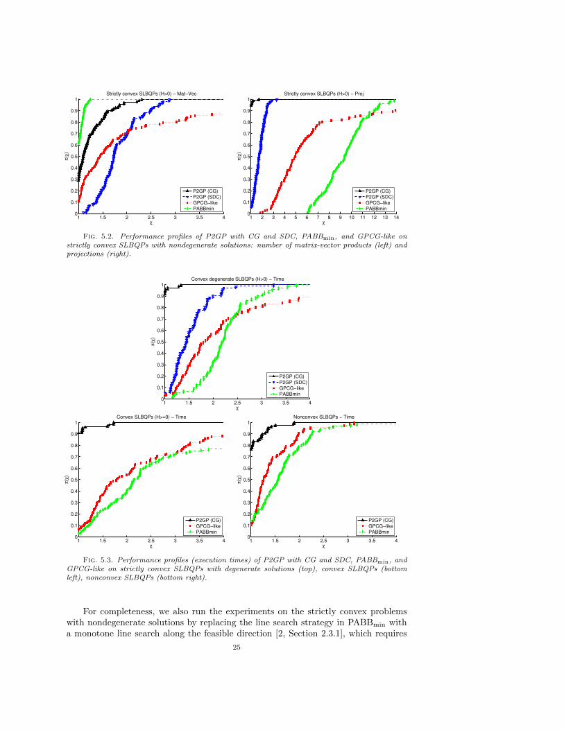
For the previous problems, the performance profiles concerning the number ofmatrix-vector products and the number of projections are also shown, in Figure 5.2.We see that PABBmin performs the smallest number of matrix-vector products, fol-

23

1 1.5 2 2.5 3 3.5 40

0.1

0.2

0.3

0.4

0.5

0.6

0.7

0.8

0.9

1

χ

π(χ

)

Strictly convex SLBQPs (H>0) − Time

P2GP (CG)

P2GP (SDC)

GPCG−like

PABBmin

1 1.5 2 2.5 3 3.5 40

0.1

0.2

0.3

0.4

0.5

0.6

0.7

0.8

0.9

1

χ

π(χ

)

Strictly convex SLBQPs (H>0), ncond = 4 − Time

P2GP (CG)

P2GP (SDC)

GPCG−like

PABBmin

1 1.5 2 2.5 3 3.5 40

0.1

0.2

0.3

0.4

0.5

0.6

0.7

0.8

0.9

1

χ

π(χ

)

Strictly convex SLBQPs (H>0), ncond = 5 − Time

P2GP (CG)

P2GP (SDC)

GPCG−like

PABBmin

1 1.5 2 2.5 3 3.5 40

0.1

0.2

0.3

0.4

0.5

0.6

0.7

0.8

0.9

1

χ

π(χ

)Strictly convex SLBQPs (H>0), ncond = 6 − Time

P2GP (CG)

P2GP (SDC)

GPCG−like

PABBmin

Fig. 5.1. Performance profiles of P2GP with CG and SDC, PABBmin, and GPCG-like onstrictly-convex SLBQPs with nondegenerate solutions: execution times for all the problems (topleft), for κ(H) = 104 (top right), for κ(H) = 105 (bottom left), and for κ(H) = 106 (bottom right).

lowed by P2GP with GC, and then by GPCG-like and P2GP with SDC. On the otherhand, the number of projections computed by P2GP with CG and with SDC is muchsmaller than for the other methods; as expected, the maximum number of projectionsis computed by PABBmin. This shows than the performance of the methods cannotbe measured only in terms of matrix-vector products; the cost of the projections mustalso be considered, especially when the structure of the Hessian makes the compu-tational cost of the matrix-vector products lower than O(n2). The good behavior ofP2GP results from the balance between matrix-vector products and projections.

The performance profiles concerning the execution times on the strictly convexSLBQPs with degenerate solutions, on the convex (but not strictly convex) SLBQPs,and on the nonconvex ones are reported in Figure 5.3. Of course, the version ofP2GP using the SDC solver was not applied to the last two sets of problems. In thecase of nonconvex problems, only 85% of the runs were considered, corresponding tothe cases where the values of the objective function at the solutions computed bythe different methods differ by less than 1%. P2GP with CG is generally the bestmethod, followed by GPCG-like and then by PABBmin. Furthermore, on strictlyconvex problems with degenerate solutions, P2GP with SDC performs better thanGPCG-like and PABBmin. GPCG-like is less robust than the other methods, since ithas 4 failures on the degenerate stricltly convex problems and 8 failures on the convexones. This confirms the effectiveness of the proportionality-based criterion.

24

1 1.5 2 2.5 3 3.5 40

0.1

0.2

0.3

0.4

0.5

0.6

0.7

0.8

0.9

1

χ

π(χ

)

Strictly convex SLBQPs (H>0) − Mat−Vec

P2GP (CG)

P2GP (SDC)

GPCG−like

PABBmin

1 2 3 4 5 6 7 8 9 10 11 12 13 140

0.1

0.2

0.3

0.4

0.5

0.6

0.7

0.8

0.9

1

χ

π(χ

)

Strictly convex SLBQPs (H>0) − Proj

P2GP (CG)

P2GP (SDC)

GPCG−like

PABBmin

Fig. 5.2. Performance profiles of P2GP with CG and SDC, PABBmin, and GPCG-like onstrictly convex SLBQPs with nondegenerate solutions: number of matrix-vector products (left) andprojections (right).

1 1.5 2 2.5 3 3.5 40

0.1

0.2

0.3

0.4

0.5

0.6

0.7

0.8

0.9

1

χ

π(χ

)

Convex degenerate SLBQPs (H>0) − Time

P2GP (CG)

P2GP (SDC)

GPCG−like

PABBmin

1 1.5 2 2.5 3 3.5 40

0.1

0.2

0.3

0.4

0.5

0.6

0.7

0.8

0.9

1

χ

π(χ

)

Convex SLBQPs (H>=0) − Time

P2GP (CG)

GPCG−like

PABBmin

1 1.5 2 2.5 3 3.5 40

0.1

0.2

0.3

0.4

0.5

0.6

0.7

0.8

0.9

1

χ

π(χ

)

Nonconvex SLBQPs − Time

P2GP (CG)

GPCG−like

PABBmin

Fig. 5.3. Performance profiles (execution times) of P2GP with CG and SDC, PABBmin, andGPCG-like on strictly convex SLBQPs with degenerate solutions (top), convex SLBQPs (bottomleft), nonconvex SLBQPs (bottom right).

For completeness, we also run the experiments on the strictly convex problemswith nondegenerate solutions by replacing the line search strategy in PABBmin witha monotone line search along the feasible direction [2, Section 2.3.1], which requires

25

only one projection per GP iteration. We note that this line search does not guaranteein general that the sequence generated by the GP method identifies in a finite numberof steps the variables that are active at the solution (see, e.g., [13]). Nevertheless, wemade experiments with the line search along the feasible direction, to see if it maylead to any time gain in practice. The results obtained, not reported here for the sakeof space, show that the two line searches lead to comparable times when the numberof active variables at the solution is small, i.e., naxsol = 0.1. On the other hand,the execution time with the original line search is slightly smaller when the numberof active variables at the solution is larger.

Finally, the performance profiles concerning the execution times taken by theP2GP, PABBmin and GPCG-like methods on the strictly convex BQPs with nonde-generate and degenerate solutions, on the convex (but not strictly convex) BQPs, andon the nonconvex ones are shown in Figure 5.4. Only 97% of the runs on the noncon-vex problems are selected, using the same criterion applied to nonconvex SLBQPs.P2GP with CG is again the most efficient method. The behavior of the methods issimilar to that shown on SLBQPs. However, P2GP with SDC and PABBmin havecloser behaviors, according to the smaller time required by projections onto boxes,which leads to a reduction of the execution time of PABBmin. GPCG-like has againsome failures: 6 on the strictly convex problems with nondegenerate solutions, 5 onthe ones with degenerate solutions, and 9 on the convex (but not strictly convex)problems.

Now we compare P2GP (using CG) with BLG on the random problems. BLGwas run in its full-space mode (default mode), because the form of the Hessian (5.1)does not allow to take advantage of the subspace mode. The stopping condition (4.5)was implemented in BLG, and the code was run with the same tolerance and the samemaximum numbers of matrix-vector products and projections used for P2GP. Defaultvalues were used for the remaining parameters of BLG. Of course, a comparison ofthe two codes in terms of execution time would be misleading, since BLG is written inC, while P2GP has been implemented in Matlab. Therefore, we consider the matrix-vector products. We do not show a comparison in terms of projections too, becauseBLG does a projection at each iteration, and this generally results in many moreprojections than P2GP. Performance profiles are provided in Figure 5.5. The resultsconcerning all the types of convex problems are shown together, since their profiles aresimilar. On these problems P2GP appears more efficient than BLG; we also verifiedthat the objective function values at the solutions computed by the two codes agreeon at least six significant digits and are smaller for P2GP for 70% of the test cases.Furthermore, in four cases BLG does not satisfy condition (4.5) within the maximumnumber of matrix-vector products and projections. The situation is different for thenonconvex problems, where the number of matrix-vector products performed by BLGis smaller. In this case, we verified that BLG also used Frank-Wolfe directions, whichwere never chosen for the convex problems. This not only reduced the number ofmatrix-vector products, but often led to smaller objective function values. The valuesof the objective function at the solutions computed by the two methods differ byless than 1% for only 47% of the test cases, which are the ones considered in theperformance profiles on the right of Figure 5.5. On the other hand, in three casesBLG performs the maximum number of matrix-vector products without achieving therequired accuracy.

5.4. Results on SVM problems. In order to read the SVM problems, availablein the LIBSVM format, BLG was run through the SVMsubspace code, available from

26

1 1.5 2 2.5 3 3.5 40

0.1

0.2

0.3

0.4

0.5

0.6

0.7

0.8

0.9

1

χ

π(χ

)

Strictly convex BQPs (H>0) − Time

P2GP (CG)

P2GP (SDC)

GPCG−like

PABBmin

1 1.5 2 2.5 3 3.5 40

0.1

0.2

0.3

0.4

0.5

0.6

0.7

0.8

0.9

1

χ

π(χ

)

Convex degenerate BQPs (H>0) − Time

P2GP (CG)

P2GP (SDC)

GPCG−like

PABBmin

1 1.5 2 2.5 3 3.5 40

0.1

0.2

0.3

0.4

0.5

0.6

0.7

0.8

0.9

1

χ

π(χ

)

Convex BQPs (H>=0) − Time

P2GP (CG)

GPCG−like

PABBmin

1 1.5 2 2.5 3 3.5 40

0.1

0.2

0.3

0.4

0.5

0.6

0.7

0.8

0.9

1

χ

π(χ

)Nonconvex BQPs − Time

P2GP (CG)

GPCG−like

PABBmin

Fig. 5.4. Performance profiles (execution times) of P2GP with CG and SDC, PABBmin, andGPCG-like on strictly convex BQPs with nondegenerate solutions (top left), strictly convex BQPswith degenerate solutions (top right), convex BQPs (bottom left), nonconvex BQPs (bottom right).

http://users.clas.ufl.edu/hager/papers/Software/. Since we were interestedin comparing P2GP with the GP implementation provided by BLG, SVMsubspacewas modified to have the SVM subspace equal to the entire space, i.e., to apply BLGto the full SVM problem. For completeness we also run SVMsubspace in its subspacemode (see [26]), to see what the performance gain is with this feature. In the following,we refer to the former implementation as BLGfull, and to the latter as SVMsubspace.

Following [26], BLGfull and SVMsubspace were used with their original stop-ping condition, with tolerance 10−3. P2GP was terminated when the infinity normof the projected gradient was smaller then the same tolerance. With these stop-ping criteria, the two codes returned objective function values agreeing on about sixsignificant digits, with smaller function values generally obtained by P2GP. At most70000 matrix-vector products and 70000 projections were allowed, but they were neverreached.

In Figure 5.6, left, the performance profiles (in logarithmic scale) concerning thematrix-vector products of P2GP (with CG) and BLGfull are shown. A comparisonin terms of projections and execution times is not carried out for the same reasonsexplained for the random problems. BLGfull appears superior than P2GP; on theother hand, we verified that the number of projections performed by BLG is by fargreater than that of P2GP for eight out of ten problems. However, it must be notedthat SVMsubspace is much faster than BLGfull, as shown by the performance profiles

27

1 1.5 2 2.5 3 3.5 40

0.1

0.2

0.3

0.4

0.5

0.6

0.7

0.8

0.9

1

χ

π(χ

)

Convex SLBQPs − Mat−Vec

P2GP (CG)

BLG

1 1.5 2 2.5 3 3.5 40

0.1

0.2

0.3

0.4

0.5

0.6

0.7

0.8

0.9

1

χ

π(χ

)

Nonconvex SLBQPs − Mat−Vec

P2GP (CG)

BLG

Fig. 5.5. Performance profiles of P2GP, with CG, and BLG on convex (left) and nonconvex(right) SLBQPs: number of matrix-vector products.

0 1 2 3 4 5 60

0.1

0.2

0.3

0.4

0.5

0.6

0.7

0.8

0.9

1

χ

π(2

χ)

SVM Problems − Mat−Vec

P2GP (CG)

BLGfull

0 1 2 3 4 5 60

0.1

0.2

0.3

0.4

0.5

0.6

0.7

0.8

0.9

1

χ

π(2

χ)

SVM Problems − Time

BLGfull

SVMsubspace

Fig. 5.6. Performance profiles on SVM test problems: number of matrix-vector of P2GP, withCG, and BLG (left), and execution times of BLG and SVMsubspace (right).

concerning their execution times (see Figure 5.6, right). This confirms the greatadvantage of performing reduced-size matrix-vector products in solving the subspaceproblems for this class of test cases.

6. Concluding remarks. We presented P2GP, a new method for SLBQPswhich has its roots in the GPCG method. The most distinguishing feature of P2GPwith respect to GPCG stands in the criterion used to stop the minimization phase.This is a critical issue, since requiring high accuracy in this phase can be a useless andtime-consuming task when the face where a solution lies is far from being identified.

Our numerical tests show a strong improvement of the computational performancewhen the proportionality criterion is used to control the termination of the minimiza-tion phase. In particular, the comparison of P2GP with an extension of GPCG toSLBQPs shows the clear superiority of P2GP and its smaller sensitivity to the Hessiancondition number. Thus, proportionality allows to handle the minimization phase ina more clever way. The numerical results also show that P2GP requires much fewerprojections than efficient GP methods like PABBmin and the one implemented inBLG. This leads to a significant time saving, especially when the Hessian matrix issparse or has a structure that allows the computation of the matrix-vector productwith a computational cost smaller than O(n2), where n is the size of the problem.

28

From the theoretical point of view, a nice consequence of using the proportionalitycriterion is that finite convergence for strictly convex problems can be proved even incase of degeneracy at the solution.

An interesting feature of P2GP is that it provides a general framework, allowingdifferent steplength rules in the GP steps, and different methods in the minimiza-tion phase. The encouraging theoretical and computational results suggest that thisframework deserves to be further investigated, and possibly extended to more generalproblems. For example, it would be interesting to extend P2GP to general differen-tiable objective functions or to problems with bounds and a few linear constraints.

The Matlab code implementing P2GP used in the experiments is available fromhttps://github.com/diserafi/P2GP. It includes the test problem generator de-scribed in Section 5.1.

Acknowledgments. We wish to thank William Hager for helpful discussions aboutthe use of the BLG code and for insightful comments on our manuscript. We alsoexpress our thanks to the anonymous referees for their useful remarks and suggestions,which allowed us to improve the quality of this work.

REFERENCES

[1] S. Amaral, D. L. Allaire, and K. Willcox, Optimal L2-norm empirical importance weightsfor the change of probability measure, Statistics and Computing, 27 (2017), pp. 625–643.

[2] D. P. Bertsekas, Nonlinear Programming, Athena Scientific, Belmont, MA, USA, 1999.[3] R. H. Bielschowsky, A. Friedlander, F. A. M. Gomes, and J. M. Martınez, An adaptive

algorithm for bound constrained quadratic minimization, Investigacion Operativa, 7 (1997),pp. 67–102.

[4] E. G. Birgin, J. M. Martınez, and M. Raydan, Nonmonotone spectral projected gradientmethods on convex sets, SIAM Journal on Optimization, 10 (2000), pp. 1196–1211.

[5] A. Bjorck, Numerical methods for least squares problems, SIAM, Philadelphia, PA, USA,1996.

[6] S. Bonettini, R. Zanella, and L. Zanni, A scaled gradient projection method for constrainedimage deblurring, Inverse Problems, 25 (2009), p. 015002.

[7] P. H. Calamai and J. J. More, Projected gradient methods for linearly constrained problems,Mathematical Programming, 39 (1987), pp. 93–116.

[8] P. H. Calamai and J. J. More, Quasi-Newton updates with bounds, SIAM Journal on Nu-merical Analysis, 24 (1987), pp. 1434–1441.

[9] L. Condat, Fast projection onto the simplex and the l1 ball, Mathematical Programming, 158(2016), pp. 575–585.

[10] F. E. Curtis and W. Guo, Handling nonpositive curvature in a limited memory steepestdescent method, IMA Journal of Numerical Analysis, 36 (2016), pp. 717–742.

[11] Y.-H. Dai and R. Fletcher, Projected Barzilai-Borwein methods for large-scale box-constrained quadratic programming, Numerische Mathematik, 100 (2005), pp. 21–47.

[12] , New algorithms for singly linearly constrained quadratic programs subject to lower andupper bounds, Mathematical Programming (Series A), 106 (2006), pp. 403–421.

[13] P. L. De Angelis and G. Toraldo, On the identification property of a projected gradientmethod, SIAM Journal on Numerical Analysis, 30 (1993), pp. 1483–1497.

[14] R. De Asmundis, D. di Serafino, W. W. Hager, G. Toraldo, and H. Zhang, An efficientgradient method using the Yuan steplength, Computational Optimization and Applications,59 (2014), pp. 541–563.

[15] R. De Asmundis, D. di Serafino, and G. Landi, On the regularizing behavior of the SDAand SDC gradient methods in the solution of linear ill-posed problems, Journal of Compu-tational and Applied Mathematics, 302 (2016), pp. 81 – 93.

[16] R. De Asmundis, D. di Serafino, F. Riccio, and G. Toraldo, On spectral properties ofsteepest descent methods, IMA Journal of Numerical Analysis, 33 (2013), pp. 1416–1435.

[17] D. di Serafino, V. Ruggiero, G. Toraldo, and L. Zanni, A note on spectral properties ofsome gradient methods, in Numerical Computations: Theory and Algorithms (NUMTA-2016), vol. 1776 of AIP Conference Proceedings, 2016, p. 040003.

29

[18] , On the steplength selection in gradient methods for unconstrained optimization, AppliedMathematics and Computation, 318 (2018), pp. 176–195.

[19] E. D. Dolan and J. J. More, Benchmarking optimization software with performance profiles,Mathematical Programming, Series B, 91 (2002), pp. 201–213.

[20] Z. Dostal, Box constrained quadratic programming with proportioning and projections, SIAMJournal on Optimization, 7 (1997), pp. 871–887.

[21] Z. Dostal and L. Pospısil, Minimizing quadratic functions with semidefinite Hessian subjectto bound constraints, Computers and Mathematics with Applications, 70 (2015), pp. 2014–2028.

[22] Z. Dostal and J. Schoberl, Minimizing quadratic functions subject to bound constraints withthe rate of convergence and finite termination, Computational Optimization and Applica-tions, 30 (2005), pp. 23–43.

[23] G. Frassoldati, L. Zanni, and G. Zanghirati, New adaptive stepsize selections in gradientmethods, Journal of Industrial and Management Optimization, 4 (2008), pp. 299–312.

[24] A. Friedlander and J. M. Martınez, On the numerical solution of bound constrained opti-mization problems, RAIRO - Operations Research, 23 (1989), pp. 319–341.

[25] , On the maximization of a concave quadratic function with box constraints, SIAM Jour-nal on Optimization, 4 (1994), pp. 177–192.

[26] M. D. Gonzalez-Lima, W. W. Hager, and H. Zhang, An affine-scaling interior-point methodfor continuous knapsack constraints with application to support vector machines, SIAMJournal on Scientific Computing, 21 (2011), pp. 361–390.

[27] W. W. Hager and H. Zhang, A new active set algorithm for box constrained optimization,SIAM Journal on Optimization, 17 (2006), pp. 526–557.

[28] , An active set algorithm for nonlinear optimization with polyhedral constraints, ScienceChina Mathematics, 59 (2016), pp. 1525–1542.

[29] P. Kamesam and R. Meyer, Multipoint methods for separable nonlinear networks, Springer,1984.

[30] H. Mohy-ud-Din and D. P. Robinson, A solver for nonconvex bound-constrained quadraticoptimization, SIAM Journal on Optimization, 25 (2015), pp. 2385–2407.

[31] J. More and G. Toraldo, Algorithms for bound constrained quadratic programming problems,Numerische Mathematik, 55 (1989), pp. 377–400.

[32] J. J. More and G. Toraldo, On the solution of large quadratic programming problems withbound constraints, SIAM Journal on Optimization, 1 (1991), pp. 93–113.

[33] P. M. Pardalos and J. B. Rosen, Constrained global optimization: algorithms and applica-tions, Springer-Verlag, New York, NY, USA, 1987.

[34] B. N. Parlett, The Symmetric Eigenvalue Problem, SIAM, Philadelphia, PA, USA, 1998.[35] T. Serafini, G. Zanghirati, and L. Zanni, Gradient projection methods for quadratic pro-

grams and applications in training support vector machines, Optimization Methods andSoftware, 20 (2005), pp. 353–378.

[36] V. N. Vapnik and S. Kotz, Estimation of dependences based on empirical data, vol. 40,Springer-Verlag, New York, NY, USA, 1982.

[37] Y. Yuan, A new stepsize for the steepest descent method, Journal of Computational Mathe-matics, 24 (2006), pp. 149–156.

30