1

A Two-Stage Stochastic Programming

with Recourse Model for Determining

Robust Planting Plans in Horticulture

Ken Darby-Dowman(1)

Simon Barker(1)

Eric Audsley(2)

David Parsons(2)

(1) Department of Mathematics & Statistics, Brunel University, Uxbridge, Middlesex UB8 3PH England (2) Silsoe Research Institute, Wrest Park, Silsoe, Bedford MK45 4HS England

Corresponding author: Ken Darby-Dowman

Tel: +44 1895 203273

Fax: +44 1895 203303

E-mail: mastkhd@brunel.ac.uk

Submitted to Journal of Operational Research Society

December 1998

Resubmitted July 1999

2

Abstract

A two-stage stochastic programming with recourse model for the problem of

determining optimal planting plans for a vegetable crop is presented in this paper.

Uncertainty caused by factors such as weather on yields is a major influence on many

systems arising in horticulture. Traditional linear programming models are generally

unsatisfactory in dealing with the uncertainty and produce solutions that are

considered to involve an unacceptable level of risk. The first stage of the model relates

to finding a planting plan which is common to all scenarios and the second stage is

concerned with deriving a harvesting schedule for each scenario. Solutions are

obtained for a range of risk aversion factors that not only result in greater expected

profit compared to the corresponding deterministic model but also are more robust.

Keywords: linear programming; stochastic programming; agriculture; planning.

3

Introduction Linear and integer programming models have, for many years, been successfully

developed in many application sectors. This success has been achieved despite the fact

that very few decision problems are completely free from uncertainty. Deterministic

models with constant parameter values substituted for uncertain coefficients do not

fully model a real life system but nevertheless may well provide useful answers and

insights into the decision areas being investigated. However, there are important areas

for which the approach is unsatisfactory. Financial applications in general and

portfolio selection in particular are obvious examples and have received widespread

coverage among researchers1,2,3.

In the presence of uncertainty, many realisations of a given system are generally

possible. In such cases, a question arises over the specification of the objective

function when a deterministic optimisation model is used to represent a stochastic

system. One may wish to optimise the expected value of the objective function.

However, the resulting solution may be unstable in the sense that it might perform

poorly under some realisations whilst performing well under others. In these cases, it

may be desirable to sacrifice on optimality in order to obtain a robust solution4 that,

although sub-optimal in terms of expected value, has lower risk.

This paper concerns the treatment of uncertainty in optimisation models of

agricultural systems. The biological nature of crop production, weather and

environmental conditions and changing demand can all have considerable impact on

4

profitability for farmers and growers, as growth patterns, yields, demands and prices

are all influenced.

Many techniques have been developed for dealing with uncertainty in mathematical

programming models. Stochastic Programming with Recourse5 is a general purpose

technique that can deal with uncertainty in any of the model parameters. Mean-

Variance models6,7 and the Focus-Loss model8 deal with objective function coefficient

uncertainty. The Chance Constrained Programming approach of Charnes and Cooper9

can be adopted for right-hand-side uncertainty. A range of agricultural applications

using these respective techniques include Livestock Decisions,10 Soil Conservation,11

Crop Production8 and Irrigation Systems12.

In this paper, the problem of determining planting plans for a vegetable crop is

considered.

Background

A Brussels sprouts grower typically has a number of contracts with customers to

supply an agreed quantity of Brussels sprouts in a given size band in each week of the

harvesting season. There are many varieties of Brussels sprouts with attributes such as

marketable yield, size, maturity patterns, shape, colour, smoothness and resistance to

diseases. Each customer will hold a view as to their own preferred characteristics. For

example, for the freezer market, a smaller Brussels sprout is required compared to that

for the fresh market.

5

The planting season extends from April to June, with a harvesting period from

September up to the following March, as illustrated in Figure 1. All decisions with

regard to land use and the planting of different varieties of Brussels sprouts have to be

determined during the planting season with little indication of the actual yields for the

forthcoming year in terms of quantities and timings of development.

Planting Season Harvesting Season

April June September March

Figure 1: Planting and Harvesting Seasons

An example of a yield profile for a particular crop is shown in Figure 2. It shows how

one variety planted at a particular time and at a particular spacing is expected to grow

over a season. The graph shows the yield in tonnes per hectare in each size band if an

area of the crop is harvested in any given week. With early harvesting there is a

comparatively large quantity of the smaller size band sprouts but as the weeks

progress there is an increase in size and a peak in overall yield occurring in week 10.

The cost of harvesting depends on the crop, the harvesting week and the scenario and

is assumed to be proportional to the quantity harvested.

6

0

2

4

6

8

10

12

14

4 5 6 7 8 9 10 11 12 13

Harvesting Week

Yield(t/ha)

30-35mm

25-30mm

20-25mm

12-20mm

Figure 2: Example of a Yield Profile

Even with known yield profiles for each crop it may not be possible (or economical)

to satisfy contracts with the grower’s own yield and it is possible to buy on the open

market to make up for any shortfalls. Similarly it is possible to sell yield in excess of

that required by customer contracts on the open market. However, if the grower has a

shortfall (or surplus), it is likely that other growers will be in the same position and, as

a result, the open market price will be relatively high (or low).

A crop is defined as a particular variety of Brussels sprouts planted in a given week at

a given spacing and the problem is to decide how much of each of a set of possible

crops should be planted, where the exact yield profile is not known.

7

The Model

A linear programming model of Brussels sprouts planting and harvesting has

previously been developed by Silsoe Research Institute (SRI).13,,14 Although useful,

the main disadvantage of the model is that the recommended decisions are judged to

be too risky by growers. In other words the effects of uncertainty were not

satisfactorily addressed by these earlier models.

The major element of uncertainty that needs to be addressed here is the effect of

weather on yields. Extensive historical data is available on weather in terms of daily

temperature and precipitation at a number of locations over many years. Although

detailed historical data on yields is generally not available, there is considerable

knowledge on the relationship between weather conditions and yield.15,16 Thus

weather data for a given year at a given location can be transformed into a yield

scenario taking into account the soil type at that location. In deterministic models,

conservative assumptions are typically made when estimating parameters. In this

application, a yield profile corresponding to the 30th percentile of gross annual yields

over past years (i.e. the 7th best year out of 10) was used. In the proposed stochastic

programming (SP) model, 31 years of weather data have been used to create 31 yield

scenarios.

The 2-Stage Stochastic Linear Programming model presented here is an extension of

the BRUSPLAN model developed by Hamer14.

8

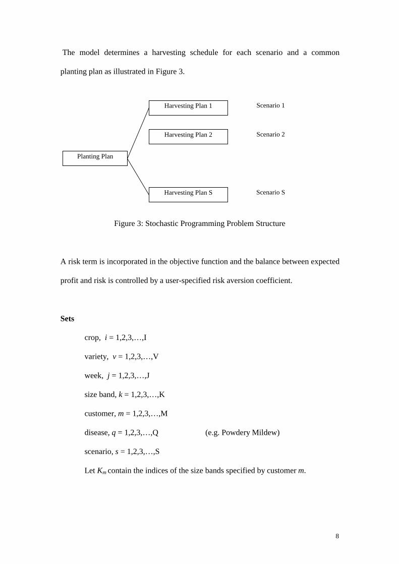
The model determines a harvesting schedule for each scenario and a common

planting plan as illustrated in Figure 3.

Figure 3: Stochastic Programming Problem Structure

A risk term is incorporated in the objective function and the balance between expected

profit and risk is controlled by a user-specified risk aversion coefficient.

Sets

crop, i = 1,2,3,…,I

variety, v = 1,2,3,…,V

week, j = 1,2,3,…,J

size band, k = 1,2,3,…,K

customer, m = 1,2,3,…,M

disease, q = 1,2,3,…,Q (e.g. Powdery Mildew)

scenario, s = 1,2,3,…,S

Let Km contain the indices of the size bands specified by customer m.

Harvesting Plan 1

Harvesting Plan S

Harvesting Plan 2

Planting Plan

Scenario 1

Scenario 2

Scenario S

9

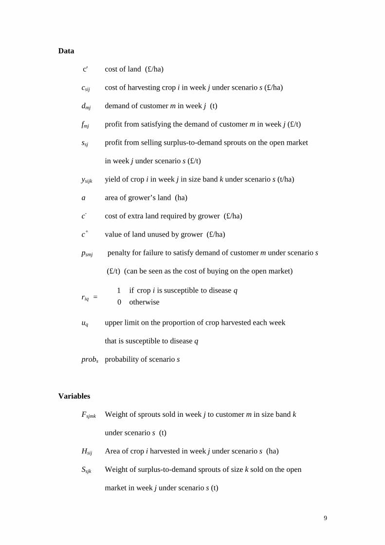
Data

′c cost of land (£/ha)

csij cost of harvesting crop i in week j under scenario s (£/ha)

dmj demand of customer m in week j (t)

fmj profit from satisfying the demand of customer m in week j (£/t)

ssj profit from selling surplus-to-demand sprouts on the open market

in week j under scenario s (£/t)

ysijk yield of crop i in week j in size band k under scenario s (t/ha)

a area of grower’s land (ha)

c- cost of extra land required by grower (£/ha)

c+ value of land unused by grower (£/ha)

psmj penalty for failure to satisfy demand of customer m under scenario s

(£/t) (can be seen as the cost of buying on the open market)

riq =

10

if crop is susceptible to diseaseotherwise

i q

uq upper limit on the proportion of crop harvested each week

that is susceptible to disease q

probs probability of scenario s

Variables

Fsjmk Weight of sprouts sold in week j to customer m in size band k

under scenario s (t)

Hsij Area of crop i harvested in week j under scenario s (ha)

Ssjk Weight of surplus-to-demand sprouts of size k sold on the open

market in week j under scenario s (t)

10

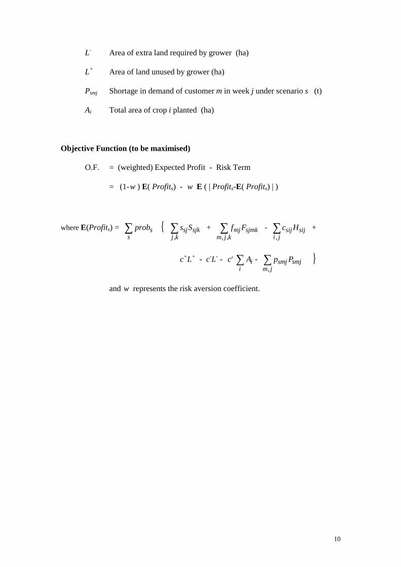
L- Area of extra land required by grower (ha)

L+ Area of land unused by grower (ha)

Psmj Shortage in demand of customer m in week j under scenario s (t)

Ai Total area of crop i planted (ha)

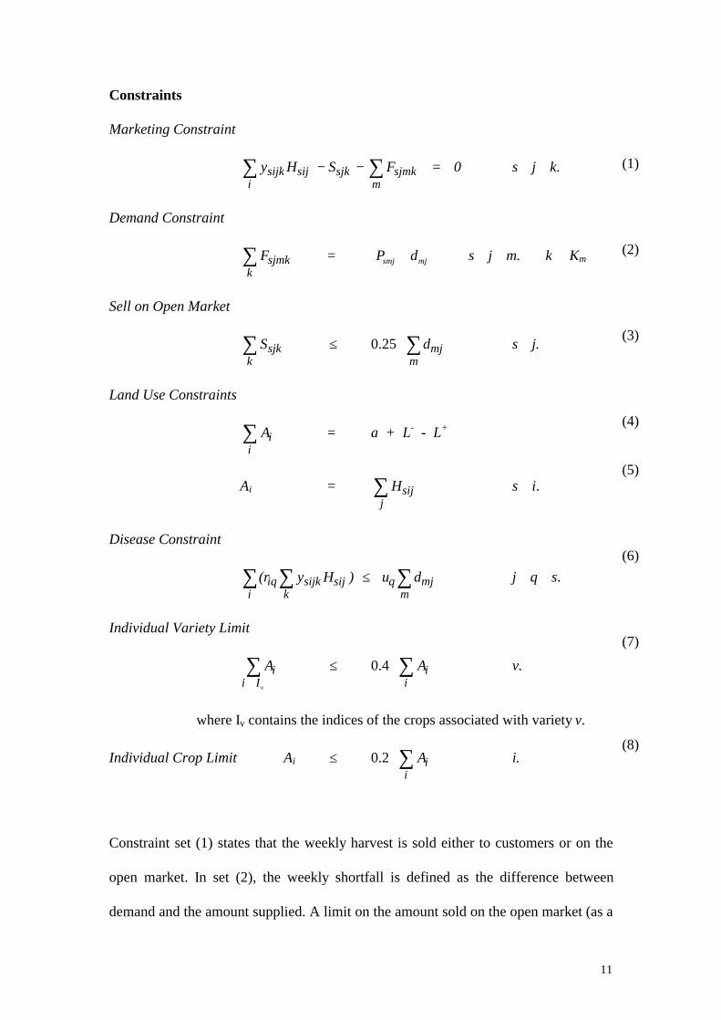
Objective Function (to be maximised)

O.F. = (weighted) Expected Profit - Risk Term

= (1-ω ) E( Profits) - ω E ( | Profits-E( Profits) | )

where E(Profits) = {probss

∑ s Ssjj k

sjk,

∑ + f Fmj sjmkm j k, ,∑ - c Hsij sij

i j,∑ +

c+L+ - c-L- - ′c Aii

∑ - p Psmj smjm j,∑ }

and ω represents the risk aversion coefficient.

11

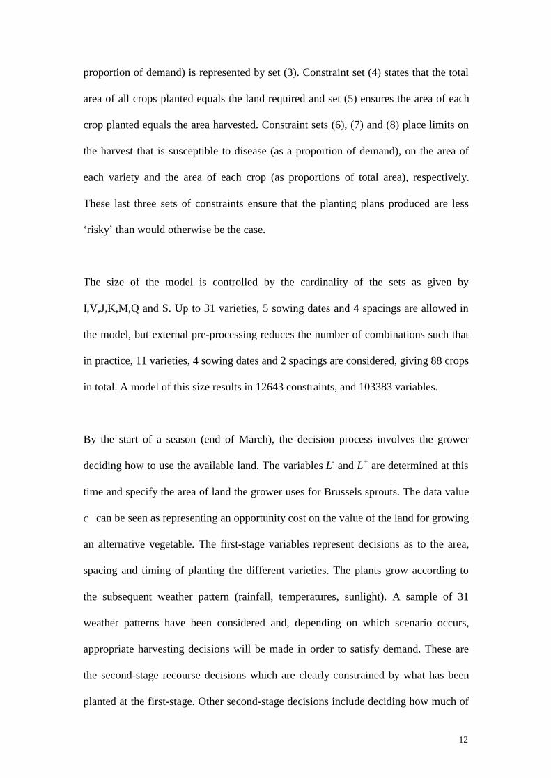
Constraints

Marketing Constraint

y H S Fsijk sij sjk sjmkmi

− − =∑∑ 0 ∀s ∀j ∀k.

Demand Constraint

Fsjmkk∑ = mjsmj dP + ∀s ∀j ∀m. k ∈ Km

Sell on Open Market

Ssjkk∑ ≤ 0.25 dmj

m∑ ∀s ∀j.

Land Use Constraints

Aii

∑ = a + L- - L+

Ai = Hsijj

∑ ∀s ∀i.

Disease Constraint

(r y H ) u diqi

sijk sijk

q mjm

∑ ∑ ∑≤ ∀j ∀q ∀s.

Individual Variety Limit

Aii Iv∈∑ ≤ 0.4 Ai

i∑ ∀v.

where Iv contains the indices of the crops associated with variety v.

Individual Crop Limit Ai ≤ 0.2 Aii

∑ ∀i.

Constraint set (1) states that the weekly harvest is sold either to customers or on the

open market. In set (2), the weekly shortfall is defined as the difference between

demand and the amount supplied. A limit on the amount sold on the open market (as a

(1)

(2)

(3)

(4)

(5)

(6)

(7)

(8)

12

proportion of demand) is represented by set (3). Constraint set (4) states that the total

area of all crops planted equals the land required and set (5) ensures the area of each

crop planted equals the area harvested. Constraint sets (6), (7) and (8) place limits on

the harvest that is susceptible to disease (as a proportion of demand), on the area of

each variety and the area of each crop (as proportions of total area), respectively.

These last three sets of constraints ensure that the planting plans produced are less

‘risky’ than would otherwise be the case.

The size of the model is controlled by the cardinality of the sets as given by

I,V,J,K,M,Q and S. Up to 31 varieties, 5 sowing dates and 4 spacings are allowed in

the model, but external pre-processing reduces the number of combinations such that

in practice, 11 varieties, 4 sowing dates and 2 spacings are considered, giving 88 crops

in total. A model of this size results in 12643 constraints, and 103383 variables.

By the start of a season (end of March), the decision process involves the grower

deciding how to use the available land. The variables L- and L+ are determined at this

time and specify the area of land the grower uses for Brussels sprouts. The data value

c+ can be seen as representing an opportunity cost on the value of the land for growing

an alternative vegetable. The first-stage variables represent decisions as to the area,

spacing and timing of planting the different varieties. The plants grow according to

the subsequent weather pattern (rainfall, temperatures, sunlight). A sample of 31

weather patterns have been considered and, depending on which scenario occurs,

appropriate harvesting decisions will be made in order to satisfy demand. These are

the second-stage recourse decisions which are clearly constrained by what has been

planted at the first-stage. Other second-stage decisions include deciding how much of

13

the harvest to supply to each customer, and buying and selling on the open market as

required for that year.

The model produces a harvesting schedule for each scenario and a single planting

plan. At the time of implementing the planting plan, it will not be known what

harvesting schedule will be required. Thus, the derived harvesting schedules are not

used and, in practice, harvesting decisions will be made by the grower in the light of

actual crop growth and market conditions as they evolve during the season.

The Objective Function is in the spirit of the E-V (Mean-Variance) approach of

Markowitz6,17 which balances expected profit against risk, using a risk aversion

coefficient ω to control the relative weighting applied to each term. The larger the

value of ω , the greater the aversion to risk. This is a MOTAD model18 (Minimisation

of Total Absolute Deviation), where the risk is measured in terms of absolute

deviations from the mean profit rather than by the variance - the advantage being it

can be modelled linearly. Hazell and Norton19 show that there is generally very little

difference between the solutions obtained using these two formulations.

It should be noted that both positive and negative deviations from the mean profit are

penalised. Counter-intuitively, this has the effect of penalising ‘good’ years with

higher-than-average profits. However, since the sum of the positive deviations about

the mean equals the sum of the negative deviations, the inclusion of only the negative

deviations is simply a matter of scaling the risk aversion coefficient. Another

approach is to consider deviations about a specified value instead of about the mean

and to minimise the sum of the absolute values of the negative deviations. In this

approach, the specified value would generally be less than the mean and would have

14

the effect of penalising the ‘worst’ years whilst not penalising years that, although

worse than the mean, are not as bad as the specified value.

Computational Aspects

Before analysing any solutions from the model, the effect of including the risk term

will be considered. Without this term, the model has the characteristic structure of a

typical two-stage stochastic programming formulation. There are constraints relating

to just the first stage variables, those relating to each scenario in the second stage and

those linking the two stages. This structure is exploited when using decomposition

techniques20 for solving large-scale stochastic linear programs. On inclusion of the

risk term, constraints are included which connect all scenarios and all the variables in

the objective function. This complicates the structure and results in an increased

solution time.

Results/Analysis

The stochastic programming model was formulated using the MPL Modelling

System21 and the deterministic equivalent problem was solved using the interior point

method of FortMP.22 The model was run for a variety of risk aversion coefficients ω

and a comparison of the various solutions obtained is made.

In order to evaluate the benefit of the stochastic programming approach compared to

the deterministic linear programming approach, a fair basis of comparison is needed.

The SP approach takes into account 31 yield scenarios corresponding to 31 years of

weather data, whereas the LP approach just considers a single yield scenario (the

15

slightly pessimistic 30th percentile year). The evaluation procedure adopted here is to

obtain a planting plan using the LP model and then run the SP model with this

planting plan fixed. The SP model then determines optimal harvesting schedules for

the specified planting plan. These results are then compared with the solution obtained

from the full SP model in which a planting plan is derived together with the

corresponding harvesting schedules.

The objective function of the model presented in the previous section maximises a

composite function comprising expected profit over scenarios and a risk term

representing the variation in profits between scenarios as measured by Mean Absolute

Deviation. The risk aversion coefficient ω determines the relative weightings

attached to the two terms. By selecting a set of increasing values of ω , a number of

solutions can be obtained that reflect decreasing risk.

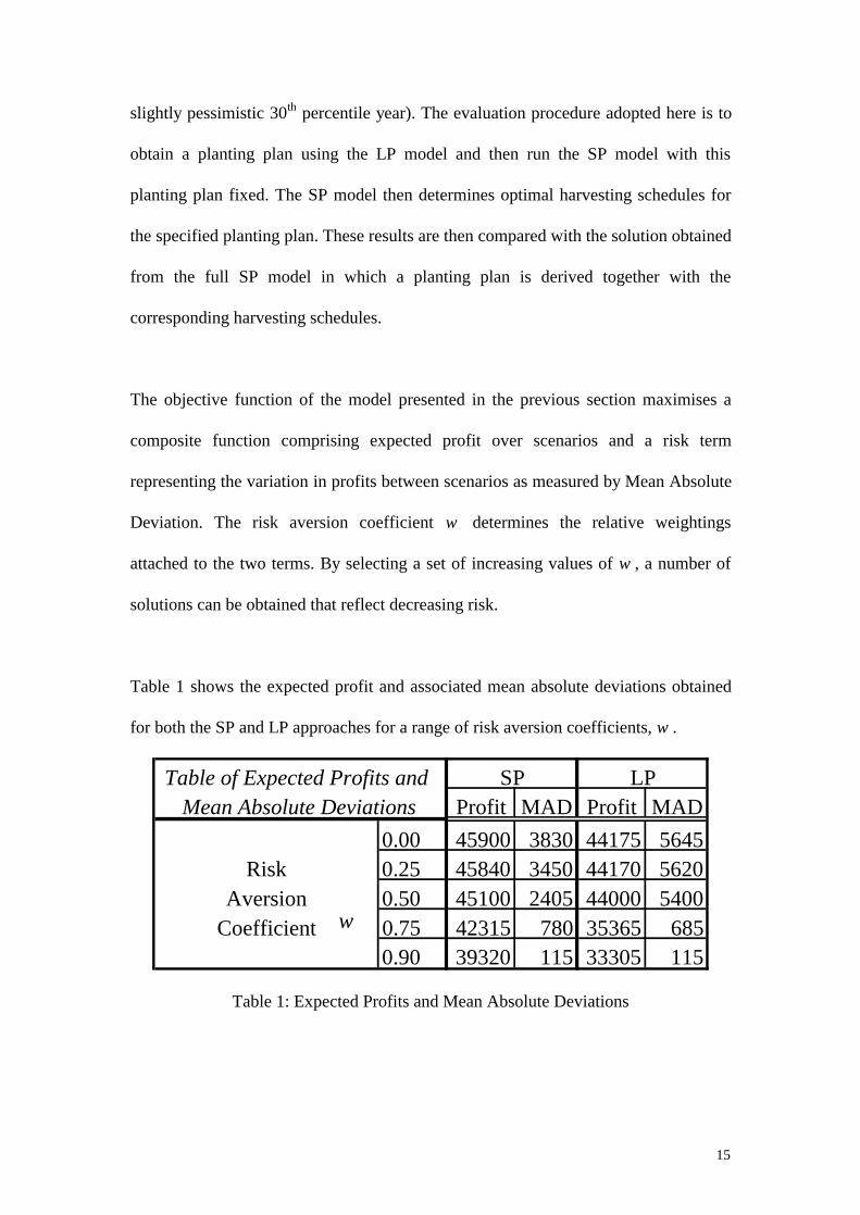
Table 1 shows the expected profit and associated mean absolute deviations obtained

for both the SP and LP approaches for a range of risk aversion coefficients, ω .

Table of Expected Profits and SP LPMean Absolute Deviations Profit MAD Profit MAD

0.00 45900 3830 44175 5645Risk 0.25 45840 3450 44170 5620

Aversion 0.50 45100 2405 44000 5400Coefficient 0.75 42315 780 35365 685

0.90 39320 115 33305 115

ω

Table 1: Expected Profits and Mean Absolute Deviations

16

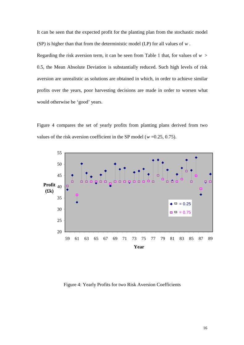
It can be seen that the expected profit for the planting plan from the stochastic model

(SP) is higher than that from the deterministic model (LP) for all values of ω .

Regarding the risk aversion term, it can be seen from Table 1 that, for values of ω >

0.5, the Mean Absolute Deviation is substantially reduced. Such high levels of risk

aversion are unrealistic as solutions are obtained in which, in order to achieve similar

profits over the years, poor harvesting decisions are made in order to worsen what

would otherwise be ‘good’ years.

Figure 4 compares the set of yearly profits from planting plans derived from two

values of the risk aversion coefficient in the SP model (ω =0.25, 0.75).

20

25

30

35

40

45

50

55

59 61 63 65 67 69 71 73 75 77 79 81 83 85 87 89

Year

Profit(£k)

= 0.25

= 0.75

Figure 4: Yearly Profits for two Risk Aversion Coefficients

ω ω

17

For ω = 0.75, there is less variation from year-to-year and there are a few years in

which a slightly greater profit is achieved. However, in the majority of years, the

profit from the planting plan corresponding to ω = 0.75 is significantly lower, and the

expected profit over all years is lower as a result. Clearly for this model, it is

preferable to have a value of ω closer to 0.25, since the benefits of good years can be

realised.

The annual profit in each of the 31 scenario years for both the LP and SP approaches

for a typical value of the risk factor is shown in Figure 5.

20

25

30

35

40

45

50

55

60

59 61 63 65 67 69 71 73 75 77 79 81 83 85 87 89Year

Profit(£k)

SPLP

Figure 5: Annual Profits for LP and SP Planting Plans (ω =0.25)

Since the LP model considers only one yield scenario, it is not surprising that it

performs poorly in some years. However in each of two years considered, 1961 and

1987, the two approaches give virtually the same (low) expected profit. These two

18

years are years of low yield and the variation in the yields associated with different

planting plans is somewhat limited. In other words the expected profit is relatively

insensitive to the planting plan. However, in other years (1964, 1973, 1974, 1980,

1981) the SP approach does significantly better than the LP approach. It is in these

years that the benefit of the SP approach is apparent when the robustness of the

solution results in substantially higher profit. Similar profiles are obtained for other

values of ω in the range 0.1 to 0.5.

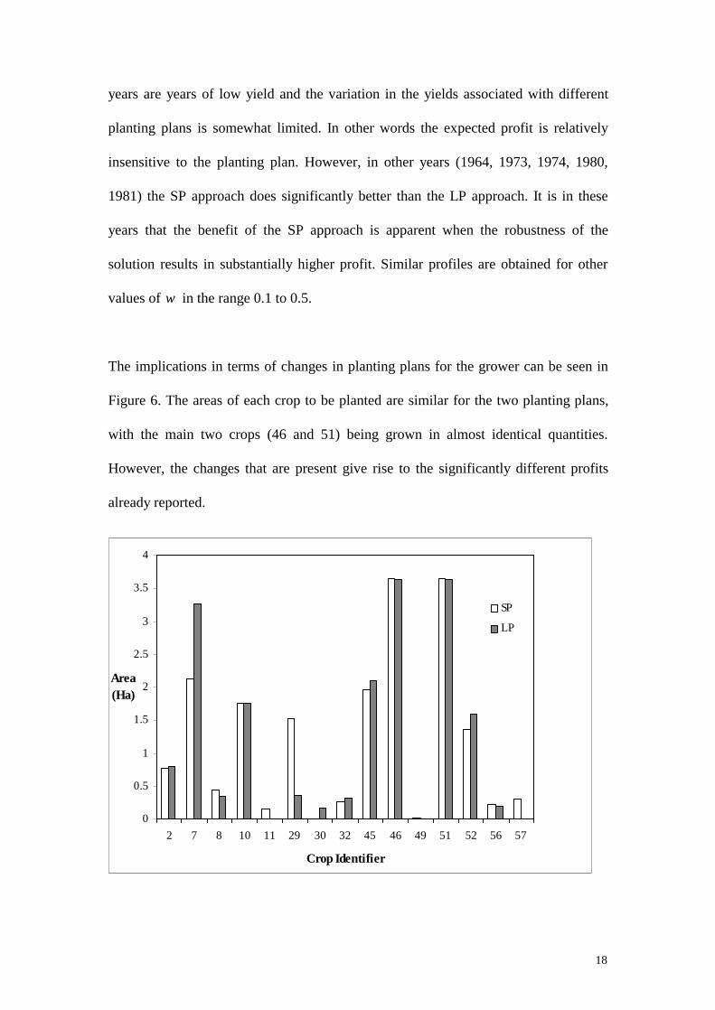
The implications in terms of changes in planting plans for the grower can be seen in

Figure 6. The areas of each crop to be planted are similar for the two planting plans,

with the main two crops (46 and 51) being grown in almost identical quantities.

However, the changes that are present give rise to the significantly different profits

already reported.

0

0.5

1

1.5

2

2.5

3

3.5

4

2 7 8 10 11 29 30 32 45 46 49 51 52 56 57

Crop Identifier

Area(Ha)

SP

LP

19

Figure 6: Comparison of Planting Plans

Modifications to the model

It is possible to make a number of refinements to the model to cater for various

practical considerations. For example, growers may require a minimum area for each

crop that they select. This means including semi-continuous variables in the model,

where the area of each crop is either 0 or not less than, say, 0.5 ha. This can be

modelled by introducing integer variables to the formulation with a resulting increase

in computational complexity. An investigation into this aspect showed little benefit

compared to a simple rounding heuristic but resulted in substantially increased

execution times. Crops where the solution value indicated planting less than 0.25 ha

were rounded to zero and those above 0.25 ha were given a lower bound of 0.5 ha.

The model could then be resolved with these values fixed, giving an appropriate new

set of harvesting decisions.

Summary

Solutions from deterministic models are unsatisfactory for many horticultural

applications, due to the high degree of uncertainty in model parameters caused,

predominantly, by the weather. The proposed stochastic programming model provides

vegetable growers with the opportunity to implement planting plans that are more

robust than would be the case with a deterministic model. The control of risk is a

20

major benefit and, as was demonstrated in the application presented in this paper,

need not result in a reduction in expected profit.

Acknowledgements Simon Barker is a research assistant funded by the

Biotechnology and Biological Sciences Research Council. The authors wish to thank

Paul Hamer for discussing his work on earlier models.

References

1. Kallberg JG, White RW and Ziemba WT (1982). Short term financial planning

under uncertainty. Management Science 28: 670-682.

2. Dantzig GB and Infanger G (1993). Multi-stage stochastic linear programs for

portfolio optimisation. Annals of Operations Research 45: 59-76.

3. Zenios SA (ed) (1993). Financial Optimisation. Cambridge University Press:

Cambridge.

4. Mulvey JM, Vanderbei RJ and Zenios SA (1995). Robust optimisation of large

scale systems. Operations Research 43: 264-281.

5. Dantzig GB (1955). Linear programming under uncertainty. Management Science

1: 197-206.

6. Markowitz HM (1952). Portfolio selection. Journal of Finance 8: 77-91.

7. Freund R (1956). The introduction of risk into a programming model.

Econometrica 21: 253-263.

21

8. Boussard J and Petit M (1967). Representative of farmer’s behaviour under

uncertainty with a focus-loss constraint. Journal of Farm Economics 49: 869-880.

9. Charnes A and Cooper WW (1959). Chance constrained programming.

Management Science 6: 73-79.

10. Lambert DK (1989). Calf retention and production decisions over time. Western

Journal of Agricultural Economics 14: 9-19.

11. Lee J, Brown DJ and Lovejoy S (1985). Stochastic efficiency versus mean-

variance criteria as predictors of adoption of reduced tillage. American Journal of

Agricultural Economics 67: 838-845.

12. Loucks D (1975). An evaluation of some linear decision rules in chance

constrained models for reservoir planning and operation. Water Resources

Research 11: 777-782.

13. Audsley E (1992). A method for selecting the optimal crops to satisfy a market

requirement. Divisional Note DN 1636, Silsoe Research Institute, UK.

14. Hamer PJC (1994). A decision support system for the provision of planting plans

for Brussels sprouts. Computers and Electronics in Agriculture 11: 97-115.

15. Hamer PJC (1992). A semi-mechanistic model of the potential growth and yield of

Brussels sprouts. Journal of Horticultural Science 67(2): 97-115.

16. Hamer PJC (1995). Modelling the effects of sowing date and plant density on the

yield and timing of development of Brussels sprouts. Journal of Agricultural

Science 124: 253-263.

17. Markowitz HM (1959). Portfolio Selection: Efficient Diversification of

Investments. John Wiley & Sons: New York.

22

18. Hazell PBR (1971). A linear alternative to quadratic and semivariance

programming for farm planning under uncertainty. American Journal of

Agricultural Economics 53: 53-62.

19. Hazell PBR and Norton RD (1986). Mathematical Programming for Economic

Analysis in Agriculture. Macmillan Publishing Co.: New York.

20. Ruszczynski A (1997). Decomposition methods in stochastic programming.

Mathematical Programming 79: 333-353.

21. Maximal Software Incorporation (1998). MPL Modelling System, Release 4.0,

USA.

22. Ellison EFD, Hajian M, Levkovitz R, Maros I, Mitra G and Sayers D (1996).

FortMP Manual, Brunel University, West London and NAG Ltd.

23