a variable neighborhood search with an effective local
TRANSCRIPT

Accepted Manuscript
A Variable Neighborhood Search with an Effective Local Search for Uncapa-
citated Multilevel Lot-Sizing Problems
Yiyong Xiao, Renqian Zhang, Qiuhong Zhao, Ikou Kaku, Yuchun Xu
PII: S0377-2217(13)00848-5
DOI: http://dx.doi.org/10.1016/j.ejor.2013.10.025
Reference: EOR 11941
To appear in: European Journal of Operational Research
Received Date: 4 May 2012
Accepted Date: 8 October 2013
Please cite this article as: Xiao, Y., Zhang, R., Zhao, Q., Kaku, I., Xu, Y., A Variable Neighborhood Search with
an Effective Local Search for Uncapacitated Multilevel Lot-Sizing Problems, European Journal of Operational
Research (2013), doi: http://dx.doi.org/10.1016/j.ejor.2013.10.025
This is a PDF file of an unedited manuscript that has been accepted for publication. As a service to our customers
we are providing this early version of the manuscript. The manuscript will undergo copyediting, typesetting, and
review of the resulting proof before it is published in its final form. Please note that during the production process
errors may be discovered which could affect the content, and all legal disclaimers that apply to the journal pertain.
1
A Variable Neighborhood Search with an Effective Local Search for
Uncapacitated Multilevel Lot-Sizing Problems
Yiyong Xiao1, Renqian Zhang2, Qiuhong Zhao3,�, Ikou Kaku4, Yuchun Xu5
1School of Reliability and Systems Engineering, Beihang University, Beijing, 100191, China
E-mail: [email protected] of Economics and Management, Beihang University, Beijing, 100191, China
E-mail: [email protected] of Economics and Management, Beihang University, Beijing, 100191, China
E-mail: [email protected] of Environmental and Information studies, Tokyo City University, Tokyo Japan
E-mail: [email protected] 5School of Applied Sciences, Cranfield University, Cranfield, Bedford, MK43 0AL, UK
E-mail: [email protected]
Abstract: In this study, we improved the variable neighborhood search (VNS) algorithm for solving uncapacitated
multilevel lot-sizing (MLLS) problems. The improvement is two-fold. First, we developed an effective local search
method known as the Ancestors Depth-first Traversal Search (ADTS), which can be embedded in the VNS to
significantly improve the solution quality. Second, we proposed a common and efficient approach for the rapid
calculation of the cost change for the VNS and other generate-and-test algorithms. The new VNS algorithm was
tested against 176 benchmark problems of different scales (small, medium, and large). The experimental results
show that the new VNS algorithm outperforms all of the existing algorithms in the literature for solving
uncapacitated MLLS problems because it was able to find all optimal solutions (100%) for 96 small-sized problems
and new best-known solutions for 5 of 40 medium-sized problems and for 30 of 40 large-sized problems.
Key Words: Metaheuristics; Multilevel lot-sizing (MLLS) problem; ADTS local search; Variable Neighborhood
Search (VNS)
1. Introduction
The multilevel lot-sizing (MLLS) problem addresses how to best determine the trade-off cost in a production
system with the purpose of satisfying customer demand with a minimum total cost. The MLLS problem plays an
important role in modern production systems of manufacturing and assembly firms. Many planning systems, such as
Material Request Planning (MRP) and Master Product Scheduling (MPS), depend heavily on the basic
mathematical model and solution approaches for the MLLS problem. Nevertheless, the MLLS problem was proven
to be strongly NP-hard (Arkin et al., 1989). Optimal solutions to large-sized problems with complex product
structures are notably difficult to find. In addition, optimal algorithms exist only for small-sized MLLS problems,
and these algorithms include dynamic programming formulations (Zangwill, 1968, 1969), an
assembly-structure-based method (Crowston and Wagner, 1973), and branch-and-bound algorithms (Afentakis et
al., 1984; Afentakis and Gavish, 1986). Many heuristic approaches have been developed to solve the MLLS
problem and its variants with near-optimal solutions. Early studies first applied sequential applications of
single-level lot-sizing models to each component of the product structure (Yelle, 1979; Veral and LaForge, 1985),
Correspoding author.Address: 37 Xueyuan Road, Haidian District. Beijing 100191, China. Tel.: +86 10 82316181; fax: +86 10 82328037. E-mail address: [email protected] (Q.H. Zhao)
2
and later studies used an approximate application of multilevel lot-sizing models (Blackburn and Millen, 1982,
1985; Coleman and McKnew, 1991).
The uncapacitated MLLS acts as a fundamental problem, and its solution approach could be highly meaningful to
many of its extended versions, including the capacitated MLLS, the MLLS with time-windowing, and the MLLS
with order acceptance. In practice, many SME firms in China’s electromechanical industry are more willing to adopt
dynamic capability policies because they can improve their capacities during busy seasons with many methods,
such as extra working-time, temporal employment, and rented machines. Therefore, the uncapacitated MLLS model
caters to the situations of their ERP systems.
Over the past decade, several metaheuristic algorithms have been developed to solve uncapacitated MLLS
problems with complex product structures. It has been reported that these algorithms are capable of providing highly
cost-efficient solutions with a reasonable computing load. Dellaert and Jeunet (2000) and Dellaert et al. (2000) first
presented a hybrid genetic algorithm (HGA) for solving uncapacitated MLLS problems with a general product
structure and introduced a competitive strategy for mixing the use of five operators in the evolution of the
chromosomes from one generation to the next. Homberger (2008) presented a parallel genetic algorithm (PGA) and
an empirical policy for deme migration (rate, interval, and selection) for the MLLS problem. These researchers used
the power of parallel calculations to decentralize the large calculation load over multiple processors (30 processors
were used in their experiments). In addition to genetic algorithms, other metaheuristic algorithms, such as simulated
annealing (SA) algorithms (Tang, 2004; Homberger, 2010), the particle swarm optimization (PSO) algorithm by
Han et al. (2009), the MAX-MIN ant colony optimization (ACO) system by Pitakaso et al. (2006, 2007), and the
soft optimization approach (SOA) based on segmentation by Kaku et al. (2006, 2010), have been developed for
solving uncapacitated MLLS problems.
The variable neighborhood search (VNS) algorithm initiated by Mladenovic and Hansen (1997) is a top-level
methodology for solving optimization problems. Because its principle is simple and easy to understand and
implement, various VNS-based algorithms have been successfully applied to many optimization problems (Hansen
et al., 2008a, 2008b, 2010). Mladenovic et al. (2012a) presented a new schema of the general variable neighborhood
search (GVNS), which is an extended version of the basic VNS that considers multiple neighborhood structures.
Labadie et al (2012) proposed a VNS procedure based on the idea of exploring, most of the time, granular instead of
complete neighborhoods in order to improve the algorithms efficiency without loosing effectives. A brief
summarization of recent successful VNS applications can be found in Mladenovic et al. (2012b).
Xiao et al. (2011a) first developed a VNS-based algorithm for basic schema and a shift rule to solve small- and
medium-sized MLLS problems; this algorithm performed better than the HGA in small- and medium-sized
problems. Xiao et al. (2011b) developed a reduced VNS (RVNS) combined with six SHAKING techniques to solve
large-sized MLLS problems. The term “reduced” indicates a simplified version of the classical VNS algorithm
because the local search (the most time-consuming component of VNS) was removed from the basic scheme.
Although RVNS is still a generate-and-test algorithm, it differs significantly from the single-point stochastic search
(SPSS) algorithm (Jeunet and Jonard, 2005) because it uses a systematic method to change multiple bits (with a
maximum Kmax) in the incumbent to generate a candidate, whereas the latter changes only a single bit. In the study
conducted by Xiao et al. (2012), three indices (i.e., the distance, changing range, and changing level) were proposed
for a neighborhood search based on which three hypotheses were verified and can be used as common rules to
enhance the performance of any existing generate-and-test algorithm. Using these three hypotheses, the proposed
iterated neighborhood search (INS) algorithm delivered notably good performance when tested against 176
benchmark problems.
In our previous research, the neighborhood structure is defined under a distance-based metric that measures the
distance (of two solutions) using the number of different bits, and another type of neighborhood structure based on
problem decomposition was also studied in the recent literature (Helber and Sahling, 2010; Lang & Shen, 2011;
Seeanner et al., 2013). Several decomposition methods (i.e., product-oriented, time-oriented, and resource-oriented)
combined with fix-and-optimized (or partial optimization) strategies were adapted to decompose the original
3
problem into multiple sub-problems in order to restrain the optimization to a smaller area of the binary variables.
In this paper, we developed an effective local search procedure known as the Ancestors Depth-first Traversal
Search (ADTS) for the RVNS algorithm such that the RVNS algorithm can be restored to a standard VNS. Although
the ADTS procedure adds a considerable amount of computing load to the algorithm, we successfully developed an
efficient method (known as trigger) using a new formulation of MLLS problems to rapidly calculate the change in
the objective cost during the neighborhood search process. Thus, the new VNS algorithm is both effective and
efficient in solving MLLS problems with high-quality solutions and within an acceptable computing time.
The remainder of this paper is organized as follows. In Section 2, we describe the new formulation of the MLLS
problem. In Section 3, we detail a local search procedure known as ADTS which was added to our previously
presented RVNS algorithm for effectively solving the MLLS problem. Section 4 outlines a highly efficient approach
for rapidly calculating the cost variation of the objective function as the incumbent solution changes. In Section 5,
we test the proposed algorithm on 176 benchmark MLLS problem instances of different scales (small, medium, and
large) and compare its performance with that of existing methods. Finally, Section 6 presents our concluding
remarks.
2. Problem formulation and neighborhood definition
The MLLS problem under investigation is considered an uncapacitated, discrete-time, multilevel
production/inventory system with a general product structure1 and multiple-end items. We assume that external
demands for the end items are known throughout the planning horizon and that backlog is not allowed. Below, we
present the notations used to model the MLLS problem, which also can be found in the reports by Dellaert and
Jeunet (2000) and Xiao et al. (2012). � i: Index of items, i = 1, 2, …, m� t (and t'): Index of periods, t = 1, 2, …, n� Hi: Unit inventory holding cost for item i� Si: Setup cost for item i� dit: External demand for item i in period t � Dit: Total demand for item i in period t � Cij: Quantity of item i required to produce one unit of item j
�
iΓ : The set of immediate successors of item i
�1
i−Γ : The set of immediate predecessors of item i
� li: The lead time required to assemble, manufacture, or purchase item i
The decision problem focuses on how to set the production setup for all of the items in all of the planning periods
such that the decision variable is an m×n matrix denoted as follows: � Yit: Binary decision variable addressed to capture the setup cost for item i in period t.
Depending on the decision variable, two other important variables are addressed to quickly capture the inventory
holding costs. These can be introduced as follows: � Pit: The period in which the demands of item i in period t will be set for production, � Xit: The production quantity for item i in period t.
The objective function is to minimize the sum of the setup cost and the inventory holding cost for all of the items
over the entire planning horizon and is denoted by TC (total cost). We extend the formulation described by Xiao et al.
(2012) to cover the external demand for non-end items. Thus, the uncapacitated MLLS problem can be modeled as
follows:
1In a pure assembly structure, each item has multiple immediate predecessors but at most only one direct successor; in a generalstructure, each item can have multiple immediate predecessors and multiple direct successors.
4
Min. [ ]1 1
( ) ( )m n
i it i it iti t
TC Y S Y H D t P= =
= ⋅ + ⋅ ⋅ −∑∑ , (1)
s.t. {0,1}, ,itY i t∈ ∀ , (2)
{ }max 1 , ,it itP t Y t t i t′′ ′= ⋅ ≤ ≤ ∀ , (3)
, ,it
it itP tX D i t
′′=
= ∀∑ , (4)
, , ,ji
it it ij j t ljD d C X i t+∈Γ
= + ⋅ ∀∑ , (5)
0, (1 ) 0,1 , ,it it it itX X Y P n i t≥ ⋅ − = ≤ ≤ ∀ . (6)
In the above equations, Eq. (1) indicates that every item in every period will incur a setup cost, an inventory
holding cost, or nothing if a zero demand is associated with it. Please note that it is no longer necessary to calculate
the inventory levels of the items in the new model, which saves a substantial amount of computational effort. Eq. (2)
states that the decision variables for the production setup Yit are binary, and Eq. (3) states that the demands of item i
in period t are always set for the production in its closest setup period (indicated by Yit'=1) prior to period t (indicated
by t' ≤ t). Apparently, the relationship tPit ≤≤1 holds such that backlog is not allowed. Eq. (4) states that the total
demand for item i in period t includes both its external demand and the sum of the lot sizes of its direct successors
(items in iΓ ) multiplied by the production ratio with a lead time correction. Eq. (5) guarantees that the lot size of
item i in period t will cover all of the latter periods of the demands that have been set for production in period t
(indicated by Pit’ = t). Eq. (6) guarantees that the lot size is non-negative and can only be positive in the periods in
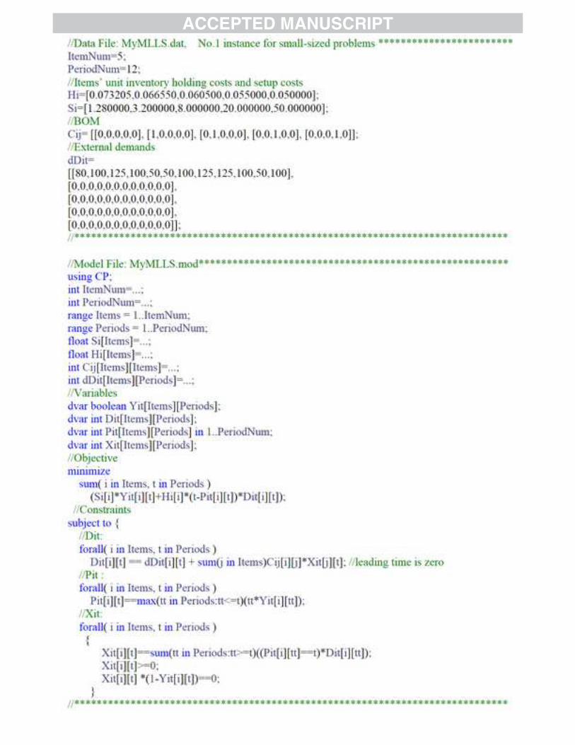
which production has been set up, which is useful for solving the mathematical programming model with certain
commercial solvers. Fig. A1 in the Appendix section shows an example of solving this programming model using
IBM ILOG CPLEX 12.2.
Based on the newly formulated model, we obtain selected properties that can be used to develop efficient
heuristic rules that may aid the algorithm in finding better solutions and enhance the search efficiency.
Property 1 Feasibility validation:
, 0, 0 ,iti P it itY D if D i t⋅ > > ∀ . (7)
This property can be read as all positive demands have been set up for production in their corresponding periods.
Property 2 Cost uniqueness:
( ) 0, ,it itY t P i t⋅ − = ∀ , (8)
which indicates that the setup cost and the inventory holding cost cannot synchronously occur in the same period of
time for an item.
Property 3. Backlog forbiddance:
1 itP t≤ ≤ , ,i t∀ , (9)
which indicates that all of the demands must be set for production in the period prior to or equal to the demand
period. Pit cannot be zero or negative.
Property 4. No demand no setup: The optimal solution of an MLLS problem satisfies
0, 0, ,it itY if D i t= = ∀ . (10)
5
Proof: Suppose that Y is the optimal solution of an MLLS problem and that there is a bit Yit�Y that violates this
property by Yit=1 and Dit=0. If we can change Y into Y' by setting Yit←0 and Yi,t+1←1, we can state that TC(Y') is
lower than TC(Y) because the production setup cost does not produce an increase but the inventory holding cost has
been decreased by i
i it j it jijh H X H X C−∈Γ
Δ = ⋅ − ⋅ ⋅∑ . Because the unit inventory holding cost of an item is
always greater than or equal to the sum of the inventory holding cost of all of its immediate components, we can
state that 0hΔ ≥ . Thus, the bit Yit�Y that violates this property does not exist.
Property 5. Inner corner property for assembly structure (Tang, 2004):
, , , ,jit j t L iY Y i t and j −
′−≥ ∀ ∈Γ . (11)
Proof: For an assembly product structure without an external demand of non-end items, the demand of non-end
items stems only from the lot size of its unique successor multiplied by the production ratio with a lead-time
correction. In other words, if an item i is not set up for production in period t (i.e., Yit=0), then all of its immediate
and non-immediate predecessors will have zero demand in their corresponding periods with a lead-time correction.
According to Property 4, the production setup in these periods must be zero (it cannot be 1). Thus, Property 5 holds,
and if Yit=1, Property 5 holds straightforwardly.
Property 6. Lot size relationship: The relationships below hold for a feasible solution of an MLLS problem:
( )1 1
,n n
it it itt t
X Y D i= =
⋅ = ∀∑ ∑ , (12)
( )1 1
, ,t t
it it itt t
X Y D i t′ ′ ′′ ′= =
⋅ ≥ ∀∑ ∑ , (13)
( ) , ,n n
it it it it itt t t t
Y X Y Y D i t′ ′ ′′ ′= =
⋅ ⋅ = ⋅ ∀∑ ∑ . (14)
3. VNS algorithm with an effective local search for MLLS problems
3.1 The mechanism of VNS for MLLS problems
The VNS is a top-level heuristic strategy that can be used to conduct an efficient stochastic search for better
solutions using predefined and systematic changes of neighborhoods. This approach implies a general principle of
from near to far for exploration of the neighborhoods of the incumbent solution. The underlying basis for this
principle is that, in most cases, there is always a higher probability of finding better solutions in nearby
neighborhoods rather than farther ones. Therefore, the definition of the neighborhood structures will be highly
important for the implementation of the VNS strategy to solve an optimization problem. Xiao et al. (2011a) first
introduced a distance-based definition of neighborhood structures for the MLLS problem and verified this approach
with experiments in later study (Xiao et al., 2012), which showed that the distance and the other two indices
(changing range and changing level) are highly effective factors for conducting a variable neighborhood search.
Below, we introduce the definition of distance-based neighborhood structures for the MLLS problem according to
Xiao et al. (2011a).
Definition 1. The distance metric: For a set of feasible solutions of an MLLS problem (i.e., {Y}), the distance
between any two solutions in {Y} (e.g., Y and Y') can be measured by the following:
( , ) | \ | | \ |, , { }Y Y Y Y Y Y Y Y Yρ ′ ′ ′ ′= = ∀ ∈ ,

6
where | \ |⋅ ⋅ denotes the number of different bits between Y and Y', e.g., 1 1
| \ |m n
it iti t
Y Y Y Y= =
′ ′= −∑∑ .
Next, based on Definition 1, the neighborhood structure of the incumbent solution can be defined as follows:
Definition 2. The neighborhood structures: A solution Y' belongs to the kth-neighborhood of the incumbent solution
Y (i.e., Nk (Y)) if and only if it satisfies
( , )Y Y kρ ′ = ,
which can be simply expressed as ( ) ( , )kY N Y Y Y kρ′ ′∈ ⇔ = , where k is a positive integer.
The application of the basic VNS scheme to solve the MLLS problem consists of two general phases. The first
phase includes defining a neighborhood structure, selecting an exploring sequence, initiating a solution Y0 as the
incumbent (Y�Y0), and defining a stopping condition. The second phase involves a neighborhood search loop in
which better solutions in the targeted neighborhood (from near to far) are repeatedly explored and accepted. In this
loop process, the nearest neighborhood N1(Y) is explored first (k�1); if no better solution can be found in
neighborhood Nk (Y), then the algorithm shifts to explore a farther neighborhood by setting k�k+1 until k = Kmax.
While searching for a better solution, a shaking procedure is used to randomly generate a candidate Y', and a local
search procedure is applied to look for the best solution Y" near Y'. If Y" is better than Y, then Y is moved to Y" by Y�
Y" and the algorithm continues to search Nk (Y) after setting k�1; otherwise, we set k�k+1. In Fig. 1, we present the
basic scheme of the VNS algorithm introduced by Hansen and Mladenovic (2001).
Place Figure 1 approximately here.
3.2 An effective local search method
Previously, Xiao et al. (2011b) proposed a reduced variable neighborhood search (RVNS) algorithm for solving
the uncapacitated multi-level lot-sizing problem. The term “reduced” means that the local search component of the
basic VNS scheme was removed to increase the computational efficiency. However, in this work, we suggest an
effective local search method and add it to the RVNS algorithm because the local search method enables a
significant improvement in the search for higher-quality solutions with an acceptable increase in the computational
load.
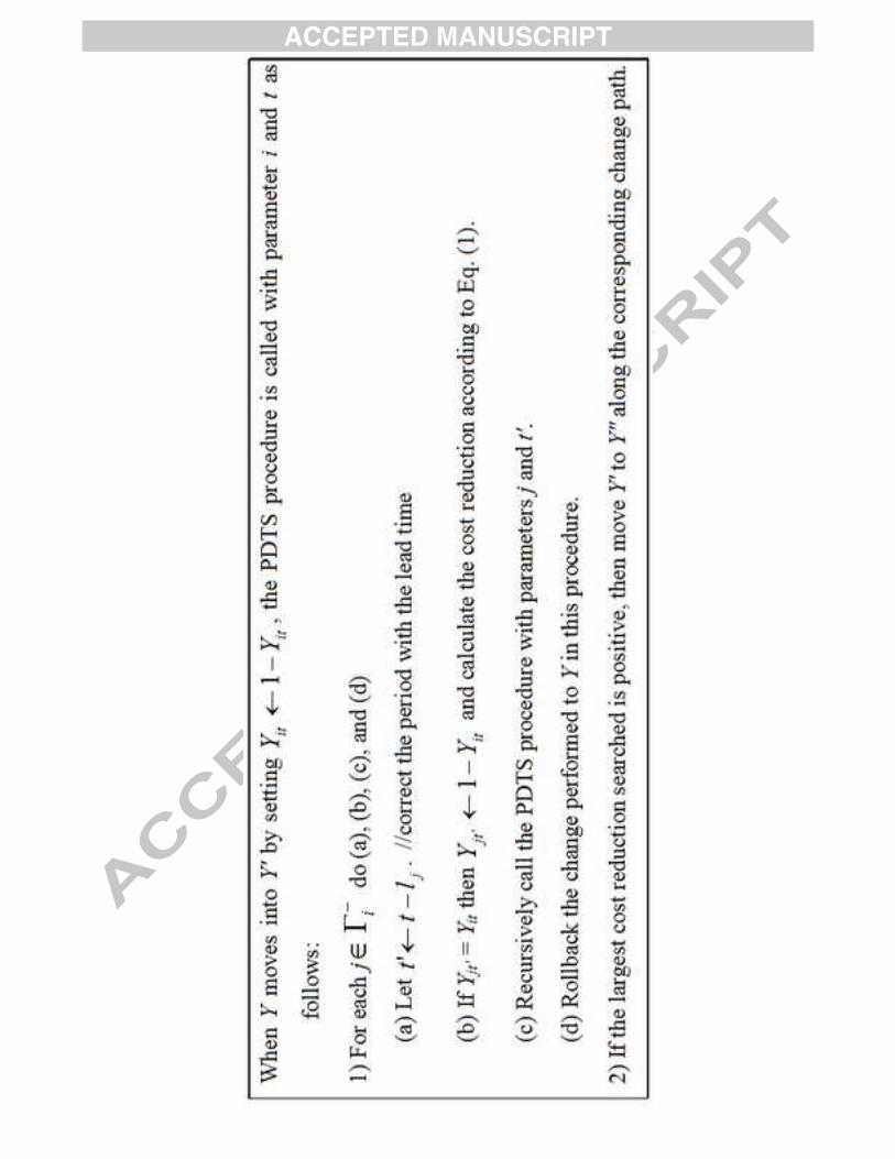
The local search method is known as the Ancestors Depth-first Traversal Search (ADTS). After shaking out a new
candidate Y' in the neighborhood Nk(Y) of the incumbent Y, we use the ADTS method to find the best solution Y"
near Y' and perform a comparison between Y and Y" (instead of Y' in RVNS) to facilitate the “move or not” decision
accordingly. In this process, the incumbent Y will tentatively move to Y' and use the ADTS to find a Y". If Y" is better
than Y', then the algorithm moves to Y"; otherwise, it returns to Y. When Y moves to Y', a total of k bits of Y must be
reversed. Once one bit (i.e., Yit) is reversed, the ADTS procedure is launched to seek the largest cost reduction by
setting (one at a time) each of the immediate and non-immediate predecessors of item i with the same setup value in
the corresponding periods of t (with a lead-time correction if the lead time is not zero). In other words, after setting
Yit←1-Yit, we use a depth-first traversal recursion to set all of the setup values of the ancestors of item i to 1-Yit and
record the path that leads to the largest cost reduction. The recorded path is exactly the method used to change Y' to
Y", which is the best solution found from a local search around Y'.
In Fig. 2, we present a simple MLLS example involving a six-item product structure over a six-period planning
horizon to illustrate the principle of ADTS. Fig. 2 (a) describes a general product structure, and Fig. 2(b) and Fig. 2
(c) present two solutions with zero lead time and one period of lead-time, respectively. Because the solution moves

7
into its kth neighborhood, it must reverse the values of the k bits that are selected randomly by the shaking procedure.
The ADTS procedure will follow each change in these bits. For example, in Fig. 2(b), once bit Y33 is reversed from
1 to 0, the ADTS procedure acts to recursively change all of its ancestors to zero and to restore the original value
through the path Y43(1→0)→Y63(unchanged)→Y43(0→1)→Y53(1→0)→Y53(0→1). In Fig. 2(c), once bit Y24 is
reversed to 1, the ADTS procedure changes and restores the bits through the path Y43(0→1)→Y62(0→1)
→Y62(1→0)→Y43(1→0) using the lead-time of 1 to correct the corresponding periods. Throughout the entire
process, the largest cost reduction and its corresponding path will be recorded, and all of the changes that the ADTS
has enacted to Y' will be restored in the end. Finally, if the largest cost reduction is positive such that the best solution
Y" found in the local search is better than Y', then the procedure moves Y' to Y" through the recorded path. The
formal description of the ADTS procedure is detailed in Fig. 3.
Place Figure 2 approximately here.
Place Figure 3 approximately here.
The concept of ADTS arose from the new formulation of the mathematical model for the uncapacitated MLLS
problem. According to Eqs. (1)-(5), when an item i changes its production setup value in period t (i.e., Yit←1-Yit),
this operation will only affect the setup and the inventory holding cost of item i and its ancestors in the affected
periods. Most of the items and periods remain in the unaffected zone. Therefore, a local search that focuses only on
the affected items and related periods will be effective for searching for the best solution close to Y'. Our
computational experiment in the latter section confirmed this conjecture and verified the effectiveness of the ADTS
method.
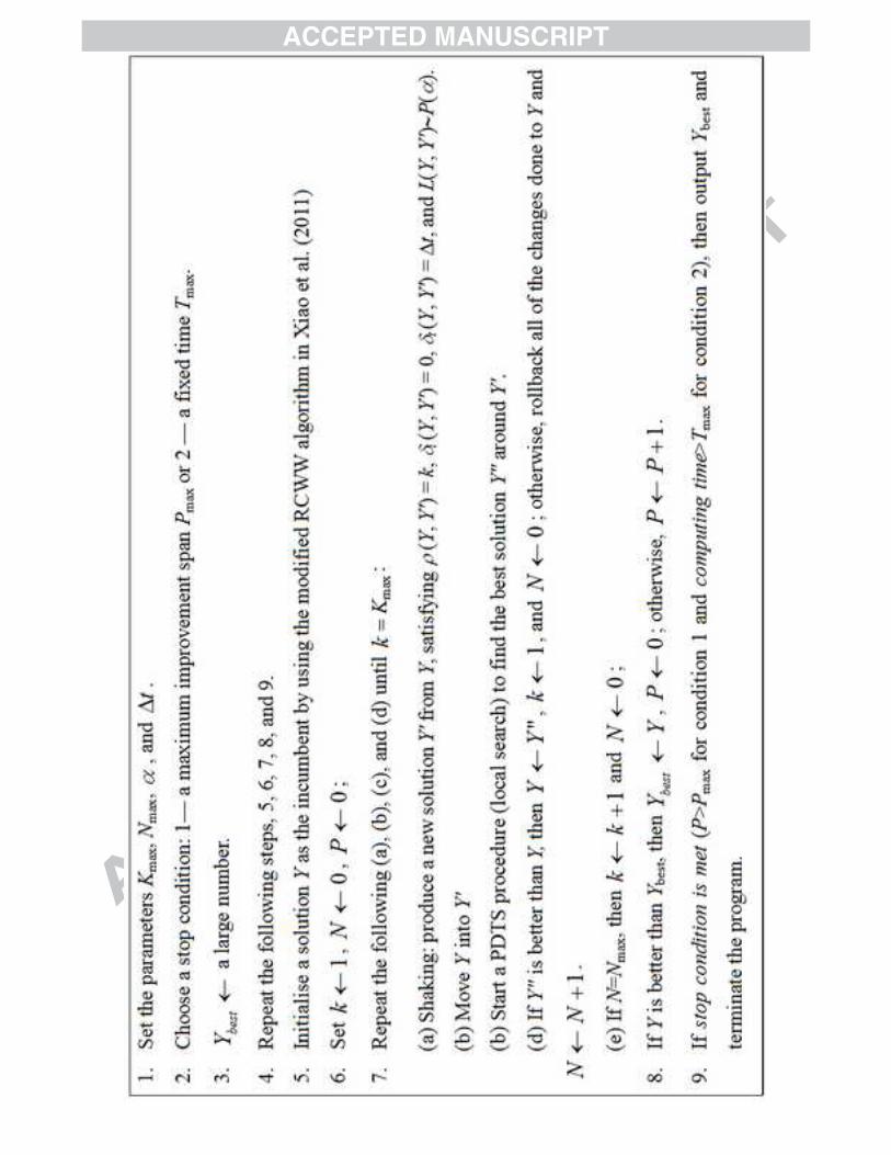
3.3 VNS algorithm with the ADTS local search
We now describe the framework of the VNS algorithm with the ADTS local search procedure, as shown in Fig 4.
This framework is based on the RVNS algorithm introduced by Xiao et al. (2011b) and was combined with the
ADTS local search procedure proposed in this study. The ideas introduced by Xiao et al. (2012) to restrain the
changing ranges and changing level in the shaking procedure were also adopted in this algorithm. This approach
represents the latest version of the neighborhood search algorithm that we developed for the MLLS problem, and we
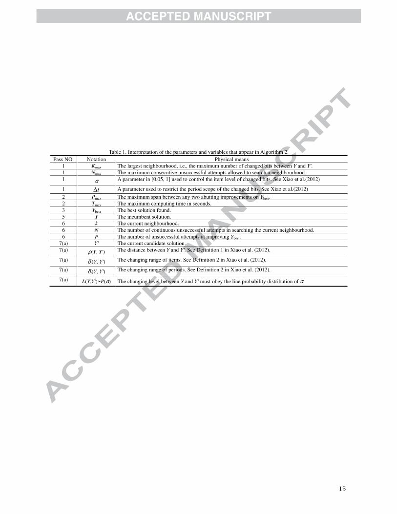
have verified its effectiveness and efficiency through the computational experiments reported in Section 5. In Table
1, we list the interpretations of the parameters and variables that appear in the VNS algorithm.
Place Figure 4 approximately here.
Place Table 1 approximately here.
The initial method is a modified RCWW (randomized cumulative Wagner and Whitin) algorithm that was first
introduced by Dellaert and Jeunet (2000) and represents a sequential use of the Wagner and Whitin (WW) algorithm
from an end item to the raw materials with a randomized cumulative production setup cost. The detailed WW
algorithm can be found in the study published by Wagner and Whitin (1958; republished in 2004). Xiao et al. (2011b)
extended the RCWW algorithm using both the modified setup cost and the modified inventory holding cost, which
are also adopted in the new VNS algorithm of this paper.
The shaking procedure in Step 7 (a) randomly produces a candidate Y from the incumbent Y', and the constraints
on distance, changing range of item/period, and changing level are controlled by the input parameters Kmax, tΔ , and
α , respectively. For additional details on these constraints, please see the manuscript by Xiao et al. (2012). Other
techniques, i.e., limiting the changed bits between the first period and the last period that have positive demand
described by Dellaert and Jeunet (2000), trigger recursive changes described by Dellaert and Jeunet (2000) and
Jeunet and Jonard (2005), setup shifting rule described by Xiao et al. (2011a), and the no demand no setup principle
described by Xiao et al. (2011b), are included in the shaking procedure. All of these techniques will help improve
the quality of the solution or the efficiency of the algorithm.
The stop condition in Step 9 can be either a maximum span between two consecutive improvements or a fixed
8
computing time elapsed. The first stop condition, i.e., a maximum improvement span Pmax, can be used for a
small-sized problem because finding the optimal solution requires only a few (or even less than 1) seconds in this
case. For medium/large-sized problems, the second stop condition, i.e., a fixed computing time, is suggested
because different problems may require considerably different computing times if using the first stop condition.
When a fixed computing time is used as the stop condition, the maximum improvement span (i.e., max(P)) can be
treated as an evaluation index that indicates the extent to which the current solution has been optimized. A small
value of max(P) indicates that the current solution still has much potential for optimization, whereas a large value
indicates that the current result is an already optimized solution of the algorithm obtained with great effort.
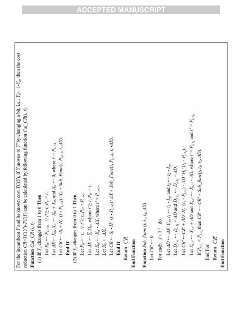
4. An efficient method for quickly calculating the cost variation
Although the ADTS local search is quite effective in searching for better solutions, it is also a notably
time-consuming procedure because it must recalculate the objective cost of the incumbent solution at each step of
the recursive path (in theory). To improve the computational load, we propose an efficient method to calculate the
cost variation of a solution change using the advantages of the new formulation for the MLLS problem shown in Eq.
(1)-Eq. (5). The new approach is a recursive accumulation of the cost reduction (or variation) (RACR in short) for
recalculation of the objective function when the incumbent solution is changed. The RACR is highly efficient
because it directly calculates the cost reduction from the changed point and the lot size in related periods.
It can be observed from Eq. (1) that the setup cost is determined only by the decision variable Y, and the inventory
holding cost is determined only by the dependent variables P and D. When a bit in Y (i.e., Yit∈Y) is changed, the
objective cost will increase by one unit of the setup cost of item i if Yit moves from 0 to 1 or decrease by one unit if
Yit moves from 1 to 0. This change also triggers subsequent changes in Pit and Xit according to Eq. (3) and Eq. (4),
respectively. Therefore, the inventory holding cost for item i will be influenced: it will increase if Yit moves from 1
to 0 or decrease if Yit moves from 0 to 1. Subsequently, the varying lot size of item i (i.e., Xit) continues to recursively
influence the demands for its immediate and non-immediate predecessors (components) in the corresponding
periods (with a lead-time correction if Li is non-zero). This scenario also causes an inventory holding cost variation.
Note that all of these changes are occurring only in the area related to the ancestors of item i (not to all of the items)
during a few periods (not in all of the periods). Therefore, the calculation of the cost reduction that results from the
related area is much faster than the complete recalculation of the objective cost for all of the items throughout all of
the periods. This insight helps us develop an efficient method for calculating the cost reduction in the neighborhood
search and may also be applicable for any other generate-and-test algorithms to enhance their computing
efficiencies. In Fig. 5, we provide the detailed steps of the RACV procedure when the incumbent Y moves to Y'.
Place Figure 5 approximately here.
We note that the efficiency of the algorithms shown in Fig. 3 and Fig. 5 can be reciprocally related to the
complexity of the product structure because the algorithm must call the recursive function to traverse the entire
ancestor tree of the changed item. Therefore, the number of ancestor tree nodes can be used to measure the
complexity of the product structure, which will considerably influence the computing efficiency. We use the
notation Ti to denote the number of ancestor tree nodes of item i and accordingly define a complexity index (CI) of
the product structure using the average number of ancestor tree nodes for all of the items as follows:
1
1 m
ii
CI Tn =
= ∑ (15)
5. Computational experiments
5.1 Problem instances and test environment
9
Three classes of uncapacitated MLLS problems of different scales (small, medium, and large) were used to test
the performance of the new VNS algorithm with the ADTS local search. Class 1 consists of 96 small-sized MLLS
problems involving a five-item assembly structure over a 12-period planning horizon, as developed by Coleman and
McKnew (1991) based on the work of Veral and LaForge (1985) and Benton and Srivastava (1985). Class 2 consists
of 40 medium-sized MLLS problems involving 40/50-item product structures over a 12/24-period planning horizon,
based on the product structures proposed by Afentakis et al. (1984), Afentakis and Gavish (1986), and Dellaert and
Jeunet (2000). Class 3 covers 40 large-sized problems with a size of 500 items over 36/52 periods, as synthesized by
Dellaert and Jeunet (2000) and used as a benchmark by Pitakaso et al. (2007), Homberger (2008, 2010), and Xiao et
al. (2011b, 2012). Thus, a total of 176 problem instances will be used to test the VNS algorithm. For the 136
problems classified as Class 1 and Class 2, the lead times of the items were all set to 0, whereas the lead times for all
of the items in the 40 large-sized problems were set to 1.
The VNS algorithm was coded in VC++6.0 and run on a PC computer equipped with an Intel(R) Core(TM)
3i-2100 3.1G CPU operating under a Windows 7 system. We used the maximum improvement span as the stop
condition for the small-sized problems in Class 1 and a fixed computing time as the stop condition for all of the
medium and large-sized problems in Class 2 and Class 3. We compared the performances of the VNS with those of
six other existing algorithms in the literature: the hybrid genetic algorithm (HGA) developed by Dellaert and Jeunet
(2000), the MAX-MIN ant system (MMAS) developed by Pitakaso et al.(2007), the parallel genetic algorithm
(PGA) developed by Homberger (2008), the ant colony algorithm (SACO) developed by Homberger and Gehring
(2009), the RVNS developed by Xiao et al. (2011b), and the ISN algorithm developed by Xiao et al. (2012).
Interested readers can download all of our experimental data, including the benchmark problems, experimental
outcomes, best solution found, executable program, and source code in VC ++6.0, from the following website:
http://semen.buaa.edu.cn/Teacher/Templet/DefaultDownLoadAttach.aspx?cwid=1224.
5.2 Computational experiments
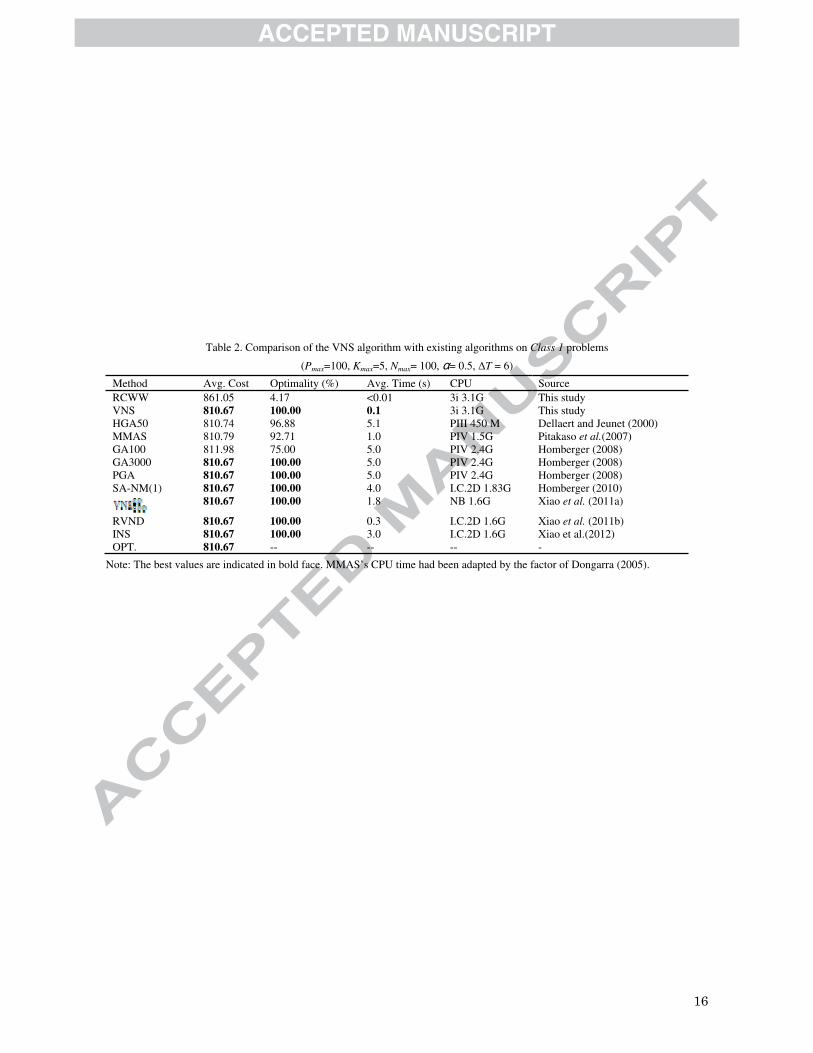
First, we ran the VNS algorithm once for the Class 1 problems using the control parameters Pmax=100, Kmax=5,
Nmax= 100, α= 0.5, and ΔT = 6. The parameter Pmax=100 indicates that the algorithm stops after 100 consecutive
attempts to improve Ybest without success. The average results are shown and compared with those of the existing
algorithms in Table 2. It can be observed that the VNS algorithm is able to discover the optimal solutions for 100%
of the 96 small-sized problems within a rather short computing time (much less than one second).
Place Table 2 approximately here.
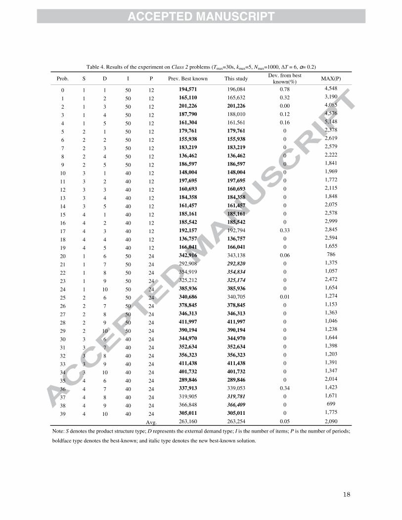
Second, we ran the VNS algorithm once for the 40 problems classified as Class 2 using the control parameters
Tmax=30 (seconds), Kmax=5, Nmax= 1000, α= 0.5, and ΔT = 6. The parameter Tmax=30 s indicates that the algorithm
stops after 30 seconds have elapsed. The average results are shown and compared with those of the existing
algorithms in Table 3, and the detailed results are listed in Table 4 and compared with the previous best-known
solutions (to date). It can be observed from Table 3 that the VNS algorithm delivers the best performances among all
of the compared algorithms with respect to the Average Cost, Deviation from the best-known (%), and the
best-known found (%). The RCWW in the second row shows the average initial solutions resulting from the RCWW
method. The VNS– in the third row indicates the VNS algorithm without use of the ADTS procedure, which
demonstrates the advantages of the local search method. The fourth row (VNS (Pmax=100)) is the performance of the
VNS algorithm with the stop condition Pmax=100 (where RACR is used) and can be compared with that of the fifth
row (VNS* (Pmax=100)) (where RACR is not used, and the objective value is always fully recalculated from the
changing item toward top materials). A comparison of these two rows reveals that, when the same solution quality is
reached, the RACR method saves a marked amount of computational time. The detailed list in Table 4 indicates that
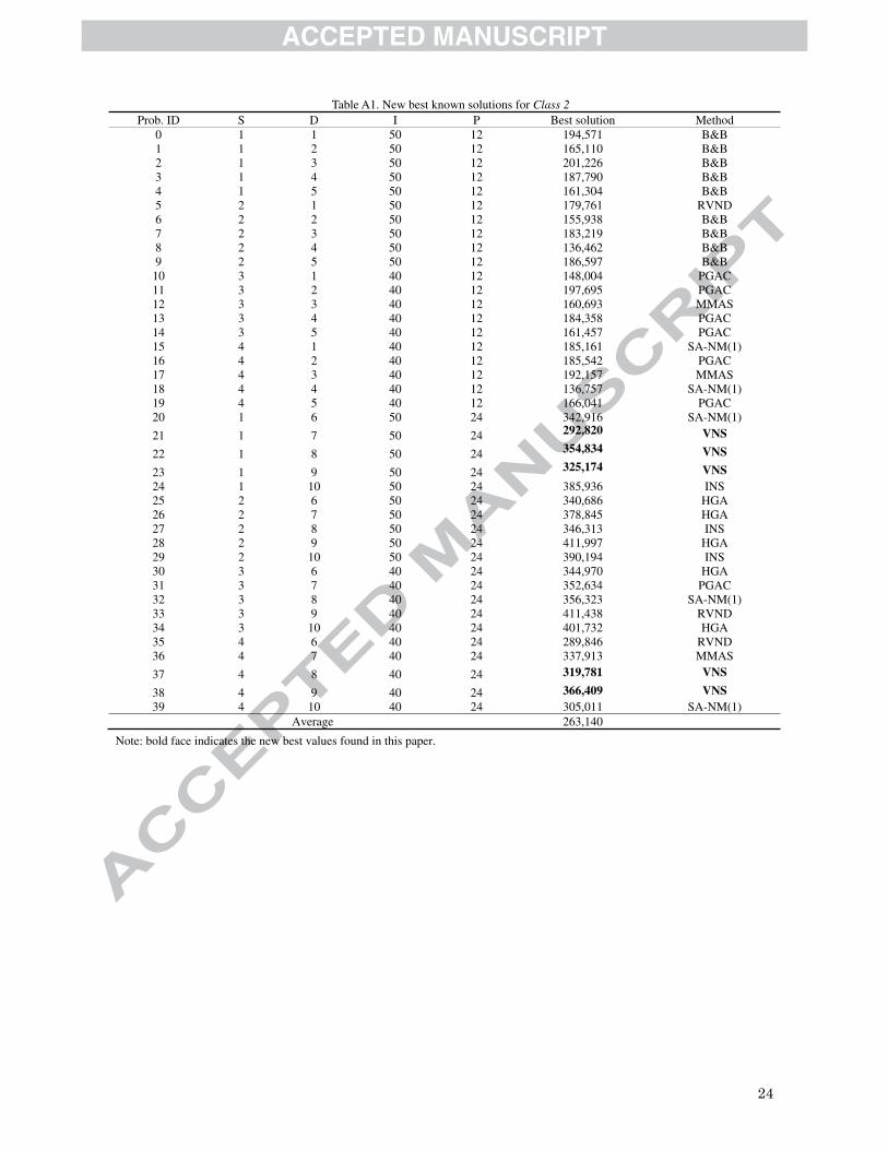
five problems were updated with new best-known solutions, and 75% of the problems (30 of 40) reached their
best-known solutions in this run. The column Max(P) in Table 4 indicates that certain problems with lower values,
such as Problems 20 and 38, could be further optimized if the maximum computing time was extended. The latest
list of best-known solutions from Class 2 problems has been updated in Table A1 in the Appendix.
10
Place Table 3 approximately here.
Place Table 4 approximately here.
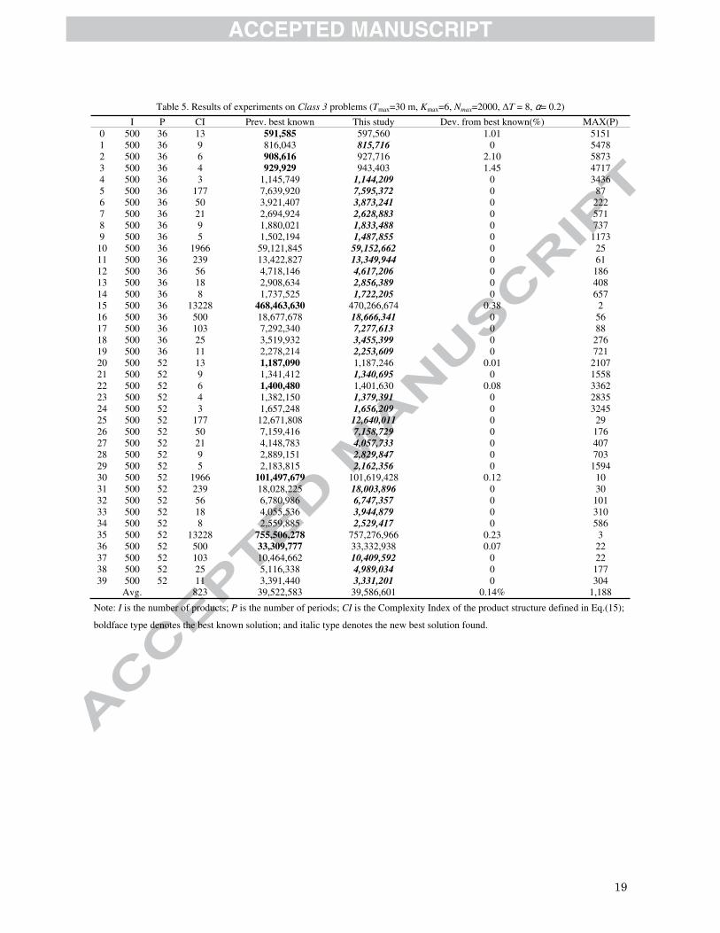
Third, we ran the VNS algorithm once on the 40 problems classified as Class 3 using the control parameters
Tmax=1800 (seconds), Kmax=6, Nmax= 2000, α= 0.5, and ΔT =8. The results are listed in Table 5. As shown in Table 5,
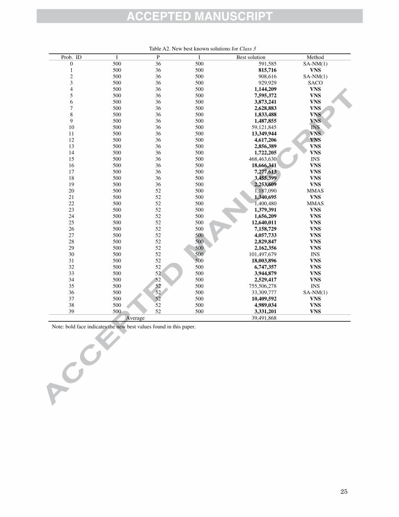
the VNS algorithm performs quite well on large-sized MLLS problems because 75% (30 out of 40) of the tested
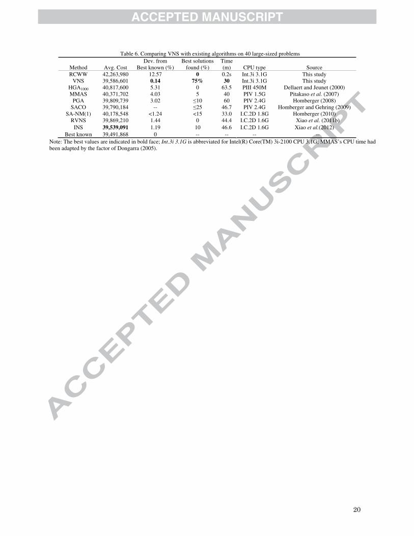
problems were updated with new best-known solutions. We summarize the results in Table 6 and compare them
with those from the existing methods in the literature. It can be observed that the VNS algorithm delivers the best
performances among all of the algorithms with respect to Deviation from Best (%) and Best solutions found (%) and
delivers the second-best performance in terms of Average Cost. It is notable that the Average Cost is the arithmetic
mean of the solutions for the 40 tested problems and is thus primarily influenced by those problems with large
objective values, e.g., Problems 15 and 35, which have the largest and second-largest objective values. If Problem
15 or 35 has a deviation from the best-known solution of merely 0.2% (increase in the objective value), this
deviation will cover up all of the good performances (decrease in the objective value) from the remaining 38
problems in terms of Average Cost for the entire problem class. For this reason, although the VNS algorithm
updated 30 of the 40 problems with new best-known solutions (Problems 15 and 35 were not updated), the Average
Cost is not the lowest among all of the existing methods. The numbers in column CI of Table 5, as defined in Eq. (15)
in Section 4, indicate the complexity of the product structures of the problems. The experimental results show that a
notably large CI can greatly decrease the efficiency of the ADTS local search method and will also result in a low
value for Max(P), which may indicate that the current solution is still far from the optimal solution and has potential
for further optimization. For example, Problems 15 and 35 are associated with a large CI and therefore output a
small Max(P); it is therefore assumed that better solutions would be very likely to be obtained if the computational
times are extended. The latest version of the best-known solutions for Class 3 problems has been updated in Table
A2 in the Appendix. An example of the new best solution of the NO.39 instance of Class 3 can be found at
http://semen.buaa.edu.cn/Teacher/Templet/DefaultDownLoadAttach.aspx?cwid=1224.
Place Table 5 approximately here.
Place Table 6 approximately here.
In Table 7, we show a comparison of the total number of evaluated candidate solutions throughout the search
process, which demonstrates the logic and computational effort defined by Alba et al. (2002) that a
generate-and-test algorithm uses to reach the best-found solution. The penultimate row in Table 7 (VNS’s shaking
solutions) is the total number of candidate solutions generated by the shaking procedure, i.e., the number of Y'. The
last row (VNS’s bit changes) in Table 7 shows the total number of times that one bit change (including 1→0 and
0→1) occurred in the incumbent solution, which are the shifts that primarily conducted by the shaking procedure of
VNS (Y→Y') and the ADTS procedure (Y'→Y"). The comparison in Table 7 shows that, although the VNS
algorithm delivered the best performance in terms of solution quality, it required much more logic and
computational effort than other methods. This result demonstrates the benefits of the proposed RACR method for
the rapid calculation of the objective function when a bit change occurs. In other words, RACR enables the VNS
algorithm (and other generate-and-test algorithms, in our opinion) to test a larger number of candidate solutions
within the same computational time.
Place Table 7 approximately here.
Finally, a parameter Nmax was added to our VNS algorithm to indicate the extent to which a neighborhood should
be explored before moving to the next neighborhood by k←k+1; in contrast, in the basic scheme of the classical
11
VNS algorithm, the parameter Nmax is fixed to 1. We then performed the following experiment to verify the role of
Nmax in the VNS algorithm. We used the 40 Class 2 medium-sized problems as the benchmark problem set to test the
parameter Nmax, which was varied from 1, 10, 50, 100, 200, 500, 1000, to 2000. The other parameters were fixed at
Tmax=30 s, Kmax=5, ΔT = 6, and �= 0.2, the stop condition was fixed at 30 seconds of computing time for each
problem. The Average Cost, Deviation from best (%), and best solutions found (%) are recorded in the experiments
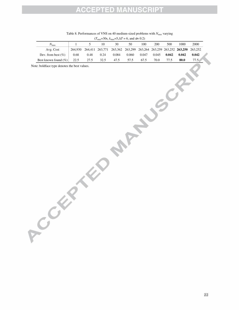
with respect to every value of Nmax. The experimental results are shown in Table 8. It can be observed that, with the
same computing time, the VNS algorithm tends to obtain a better quality of solutions as the parameter Nmax
increases. The best value for Nmax is approximately 1000, and a continued increase of Nmax to values higher than
1000 will not improve the solutions. It is notable that the solution quality is quite poor when Nmax=1, which is
exactly the case for the basic VNS scheme shown in Fig. 1 without the Nmax parameter. In Table 9, we performed
similar experiments for parameter Kmax, which was increased from 1 to 10 at intervals of 1, and the other parameters
were fixed at Tmax=30 s, Nmax=1000, ΔT = 6, and � = 0.2. The experimental results are shown in Table 9. It can also
be observed that the VNS algorithm tends to obtain better solutions as the parameter Kmax increases, and an optimal
value of Kmax=8, which gave even better outcomes than those observed in the previous experiments with Kmax=5
shown in Table 3, was found. We believe that a proper Kmax will also improve the solutions shown in Table 5 for the
large-sized problems, because the Kmax=6 used is relatively small. Interested readers can download our program to
perform their own experiments
(http://semen.buaa.edu.cn/Teacher/Templet/DefaultDownLoadAttach.aspx?cwid=1224). Note that when Kmax=1, the
VNS algorithm will degrade to the single-point stochastic search (SPSS) studied by Jeunet and Jonard (2005).
Several new best-known solutions were observed in the experiments, but we did not add them to the best-known list
of Table A1 because they were found using multiple runs.
Place Table 8 approximately here.
Place Table 9 approximately here.
6. Conclusions
The uncapacitated MLLS model represents a basic form of many extended versions of the MLLS problem
under various constraints. The solution approach is foundational and plays a basic role in the solution of many other
extended problems. We recently conducted studies on this problem using a variable neighborhood search and
presented certain effective and efficient techniques and algorithms. In this paper, we continue our contributions to
this topic and focus primarily on two points. First, we suggest an effective local search method that can be added to
our previously presented RVNS algorithm; as a result, the solution quality can be markedly improved because many
of the well-known benchmark problems were updated with new best-known solutions obtained from our
computational experiments. Second, a highly efficient approach for the rapid calculation of the cost variation of the
objective function when the incumbent solution is changed was presented. This approach can significantly improve
the efficiency of the VNS algorithm and, more importantly, may be helpful in improving the efficiency of many
other generate-and-test algorithms for MLLS problems that have been historically presented in the literature.
Acknowledgements
This work was supported by the National Natural Science Foundation of China under Projects No. 71271009,
71271010, and 71071007 and the Japan Society of Promotion of Science (JSPS) under Grant No. 24510192.
Appendix A
Place Figure A1 approximately here.
Place Table A1 approximately here.

12
Place Table A2 approximately here.
References Alba, E., Nebro,A.J., Troya, J.M. (2002). Heterogeneous computing and parallel genetic algorithms. Journal of Parallel Distributed
Computing, 62, 1362-1385.
Afentakis, P., Gavish, B., Kamarkar, U. (1984). Computationally efficient optimal solutions to the lot-sizing problem in multistage
assembly systems. Management Science, 30, 223-239.
Afentakis, P., Gavish, B. (1986). Optimal lot-sizing algorithms for complex product structures. Operations Research, 34, 237-249.
Arkin, E., Joneja, D., Roundy R. (1989). Computational complexity of uncapacitated multi-echelon production planning problems.
Operation Research Letters. 8, 61–66
Benton, W.C., Srivastava, R.(1985). Product structure complexity and multilevel lot sizing using alternative costing policies. Decision
Sciences, 16, 357-369.
Blackburn, J.D., Millen, R.A. (1982). Improved heuristics for multi-stage requirements planning system. Management Science, 28,
44-56.
Blackburn, J.D., Millen, R.A. (1985). An evaluation of heuristic performance in multi-stage lot-sizing systems. International Journal
of Production Research, 23, 857-866.
Coleman, B.J., McKnew, M.A. (1991). An improved heuristic for multilevel lot sizing in material requirements planning. Decision
Sciences, 22, 136-156.
Crowston, W.B., Wagner, H.M. (1973). Dynamic lot size models for multi-stage assembly system. Management Science, 20, 14-21.
Dongarra, J.J. (2005). Performance of various computers using standard linear equations software (Linpack Benchmark Report).
University of Tennessee Computer Science Technical Report, CS-89-85,
Dellaert, N., Jeunet, J.(2000). Solving large unconstrained multilevel lot-sizing problems using a hybrid genetic algorithm.
International Journal of Production Research, 38, 1083-1099.
Dellaert, N., Jeunet, J., Jonard, N. (2000). A genetic algorithm to solve the general multi-level lot-sizing problem with time-varying
costs. International Journal of Production Economics, 68, 241-257.
Hansen, P., Mladenovic, N. (2001). Variable neighborhood search: principles and applications. European Journal of Operational
Research, 130, 449-467.
Hansen, P., Mladenovic, N., Moreno-Perez, J.A. (2008a). Variable neighborhood search. European Journal of Operational Research,
191, 593-595.
Hansen, P., Mladenovic, N., Moreno-Perez, J.A. (2008b). Variable neighbourhood search: Methods and applications. 4OR-A Quarterly
Journal of Operations Research, 6 (4), 319-360.
Hansen, P., Mladenovic, N., Moreno-Perez, J.A. (2010). Variable neighbourhood search: Methods and applications. Annals of
Operations Research, 175 (1), 367-407.
Han, Y., Tang, J.F., Kaku, I., Mu, L.F. (2009). Solving uncapacitated multilevel lot-sizing problem using a particle swarm optimization
with flexible inertial weight. Computers and Mathematics with Applications, 57, 1748-1755.
Helber, S., Sahling F. (2010). A fix-and-optimize approach for the multi-level capacitated ot sizing problem. International Journal of
Production Economics, 123(2):247–56.
Homberger, J. (2008). A parallel genetic algorithm for the multilevel unconstrained lot-Sizing problem. INFORMS Journal on
Computing, 20, 124-132.
Homberger, J., Gehring, H. (2009). An ant colony optimization approach for the multi-level unconstrained lot-sizing problem.
Proceedings of the 42nd Hawaii international conference on system sciences, Hawaii; CD-ROM. p.7.
Homberger, J. (2010). Decentralized multi-level uncapacitated lot-sizing by automated negotiation. 4OR - A Quarterly Journal of
Operations Research, 8, 155-180.
Kaku, I., Xu, C.H. (2006). A soft optimization approach for solving a complicated multilevel lot-sizing problem. Proceedings of the 8th
Conference of Industrial Management, pp.3-8.
Kaku, I., Li, Z.S., Xu, C.H. (2010). Solving large multilevel lot-Sizing problems with a simple heuristic algorithm based on
segmentation. International Journal of Innovative Computing, Information and Control, 6, 817-827.
Lang, J. C., Shen, Z. J. M. (2011). Fix-and-optimize heuristics for capacitated lot-sizing with sequence-dependent setups and
substitutions. European Journal of Operational Research, 214, 595–605.
Labadie, N., Mansini, R., Melechovsky, J., & Calvo, W., R. (2012). The Team Orienteering Problem with Time Windows: An
LP-Based Granular Variable Neighborhood Search. European Journal of Operational Research, 220, 15-27.
Mladenovic, N., Urosevic, D., Hanafi, S., Ilic A. (2012a). A general variable neighborhood search for the one-commodity
pickup-and-delivery travelling salesman problem. European Journal of Operational Research, 220, 270–285.
13
Mladenovic, N., Kratica, J., Kovacevic-Vujcic, V., & Cangalovic, M. (2012b). Variable neighborhood search for metric dimension and
minimal doubly resolving set problems. European Journal of Operational Research, 220, 328–337.
Mladenovic, N., Hansen, P. (1997). Variable neighborhood search. Computers and Operations Research, 24, 1097-1100.
Pitakaso, R., Almeder, C., Doerner, K.F., Hartl, R.F. (2006). Combining population-based and exact methods for multi-level
capacitated lot-sizing problems, International Journal of Production Research, 44(22), 4755–4771.
Pitakaso, R., Almeder, C., Doerner, K.F., Hartlb, R.F. (2007). A MAX-MIN ant system for unconstrained multi-level lot-sizing
problems. Computer and Operations Research, 34, 2533-2552.
Seeanner, F., Almada-Lobo, B., Meyr, H. (2013). Combining the principles of variable neighborhood decomposition search and the
fix&optimize heuristic to solve multi-level lot-sizing and scheduling problems. Computers & Operations Research, 40, 303–317.
Tang, O. (2004). Simulated annealing in lot sizing problems. International Journal of Production Economics, 88, 173-181.
Veral, E.A., LaForge, R.L. (1985). The performance of a simple incremental lot-sizing rule in a multilevel inventory environment.
Decision Sciences, 16, 57-72.
Wagner, H.M., Whitin, T.M. (2004). Dynamic Version of the Economic Lot Size Model. Management Science, 50, 1770-1774,
Supplement.
Xiao, Y.Y., Kaku, I., Zhao, Q.H., Zhang, R.Q. (2011a). A variable neighborhood search based approach for uncapacitated multilevel
lot-sizing problems. Computers & Industrial Engineering, 60, 218-227.
Xiao, Y.Y., Kaku, I., Zhao, Q.H., Zhang, R.Q. (2011b). A reduced variable neighborhood search algorithm for multilevel uncapacitated
lot-sizing problems. European Journal of Operational Research, 214, 223-231.
Xiao, Y.Y., Kaku, I., Zhao, Q.H., Zhang, R.Q. (2012). Neighborhood search techniques for solving uncapacitated multilevel lot-sizing
problems. Computers & Operations Research, 39, 647-658.
Yelle, L.E. (1979). Materials requirements lot sizing: a multilevel approach. International Journal of Production Research� 17,
223-232.
Zangwill, W.I. (1968). Minimum concave cost flows in certain network. Management Science, 14, 429-450.
Zangwill, W.I. (1969). A backlogging model and a multi-echelon model of a dynamic economic lot size production system — A
network approach. Management Science, 15, 506-527.
14
Captions of the Figures.
Fig 1. The basic VNS scheme
Fig. 2 An example for illustrating the PDTS local search
Fig 3. Algorithm for the PDTS local search procedure
Fig 4. The VNS algorithm with a PDTS local search for the MLLS problem
Fig 5. An efficient way (RACR) to quickly calculate the cost variation
Fig A1. An example of solving the model by using IBM ILOG CPLEX 12.2.
15
Table 1. Interpretation of the parameters and variables that appear in Algorithm 2. Pass NO. Notation Physical means
1 Kmax The largest neighbourhood, i.e., the maximum number of changed bits between Y and Y'.1 Nmax The maximum consecutive unsuccessful attempts allowed to search a neighbourhood. 1
�A parameter in [0.05, 1] used to control the item level of changed bits. See Xiao et al.(2012)
1 tΔ A parameter used to restrict the period scope of the changed bits. See Xiao et al.(2012)
2 Pmax The maximum span between any two abutting improvements on Ybest.2 Tmax The maximum computing time in seconds. 3 Ybest The best solution found. 5 Y The incumbent solution. 6 k The current neighbourhood. 6 N The number of continuous unsuccessful attempts in searching the current neighbourhood. 6 P The number of unsuccessful attempts at improving Ybest.
7(a) Y' The current candidate solution. 7(a)
�(Y, Y') The distance between Y and Y'. See Definition 1 in Xiao et al. (2012).
7(a)�i(Y, Y') The changing range of items. See Definition 2 in Xiao et al. (2012).
7(a)�t(Y, Y') The changing range of periods. See Definition 2 in Xiao et al. (2012).
7(a) L(Y,Y')�P(�) The changing level between Y and Y' must obey the line probability distribution of �.
16
Table 2. Comparison of the VNS algorithm with existing algorithms on Class 1 problems
(Pmax=100, Kmax=5, Nmax= 100, �= 0.5, ΔT = 6)
Method Avg. Cost Optimality (%) Avg. Time (s) CPU SourceRCWW 861.05 4.17 <0.01 3i 3.1G This study VNS 810.67 100.00 0.1 3i 3.1G This study HGA50 810.74 96.88 5.1 PIII 450 M Dellaert and Jeunet (2000) MMAS 810.79 92.71 1.0 PIV 1.5G Pitakaso et al.(2007)GA100 811.98 75.00 5.0 PIV 2.4G Homberger (2008) GA3000 810.67 100.00 5.0 PIV 2.4G Homberger (2008) PGA 810.67 100.00 5.0 PIV 2.4G Homberger (2008) SA-NM(1) 810.67 100.00 4.0 I.C.2D 1.83G Homberger (2010)
810.67 100.00 1.8 NB 1.6G Xiao et al. (2011a)
RVND 810.67 100.00 0.3 I.C.2D 1.6G Xiao et al. (2011b)INS 810.67 100.00 3.0 I.C.2D 1.6G Xiao et al.(2012) OPT. 810.67 -- -- -- -
Note: The best values are indicated in bold face. MMAS’s CPU time had been adapted by the factor of Dongarra (2005).

Table 3. Comparing VNS with existing methods on 40 medium-sized problems
MethodAvg.Cost
Dev. from best known (%)
Best knownfound (%)
Avg.time(s) CPU type Sources
RCWW 279,258 5.71% 0 <1 Int.3i 3.1G This studyVNS 263,254 0.05 80 30 Int.3i 3.1G This studyVNS 263,316 0.07 57.5 30 Int.3i 3.1G This study, without ADTSVNS (Pmax=100) 263,275 0.06 70 2.4 Int.3i 3.1G This studyVNS*(Pmax=100) 263,275 0.06 70 135 Int.3i 3.1G This study, without RACRHGA250 263,932 0.76 10 <60 PIII 450M Dellaert and Jeunet (2000)MMAS 263,796 0.24 15 <20 PIV 1.5G Pitakaso et al. (2007)PGA 263,360 0.07 55 60 PIV 2.4G Homberger (2008)SACO 263,347 -- -- 32 PIV 2.4G Homberger and Gehring (2009)SA-NM(1) 263,292 -- -- 40 I.C.2D 1.8G Homberger (2010)
263,571 0.16 -- 26.7 NB 1.6G Xiao et al. (2011a)RVND 263,399 0.10 45 26.7 I.C.2D 1.6G Xiao et al. (2011b)INS 263,323 0.07 55 34.2 I.C.2D 1.6G Xiao et al.(2012)Best known 263,140 0 -- -- -- --
Note: The best values are indicated in bold face; Int.3i 3.1G is abbreviated for Intel(R) Core(TM) 3i-2100 CPU 3.1G; VNS- indicates the VNS algorithm without the PDTS local search; MMAS s CPU time had been adapted by the factor of Dongarra (2005).
18
Table 4. Results of the experiment on Class 2 problems (Tmax=30s, kmax=5, Nmax=1000, ΔT = 6, �= 0.2)
Prob. S D I P Prev. Best known This study Dev. from best
known(%)MAX(P)
0 1 1 50 12 194,571 196,084 0.78 4,548
1 1 2 50 12 165,110 165,632 0.32 3,190
2 1 3 50 12 201,226 201,226 0.00 4,085
3 1 4 50 12 187,790 188,010 0.12 4,576
4 1 5 50 12 161,304 161,561 0.16 5,148
5 2 1 50 12 179,761 179,761 0 2,378
6 2 2 50 12 155,938 155,938 0 2,619
7 2 3 50 12 183,219 183,219 0 2,579
8 2 4 50 12 136,462 136,462 0 2,222
9 2 5 50 12 186,597 186,597 0 1,841
10 3 1 40 12 148,004 148,004 0 1,969
11 3 2 40 12 197,695 197,695 0 1,772
12 3 3 40 12 160,693 160,693 0 2,115
13 3 4 40 12 184,358 184,358 0 1,848
14 3 5 40 12 161,457 161,457 0 2,075
15 4 1 40 12 185,161 185,161 0 2,578
16 4 2 40 12 185,542 185,542 0 2,999
17 4 3 40 12 192,157 192,794 0.33 2,845
18 4 4 40 12 136,757 136,757 0 2,594
19 4 5 40 12 166,041 166,041 0 1,655
20 1 6 50 24 342,916 343,138 0.06 786
21 1 7 50 24 292,908 292,820 0 1,375
22 1 8 50 24 354,919 354,834 0 1,057
23 1 9 50 24 325,212 325,174 0 2,472
24 1 10 50 24 385,936 385,936 0 1,654
25 2 6 50 24 340,686 340,705 0.01 1,274
26 2 7 50 24 378,845 378,845 0 1,153
27 2 8 50 24 346,313 346,313 0 1,363
28 2 9 50 24 411,997 411,997 0 1,046
29 2 10 50 24 390,194 390,194 0 1,238
30 3 6 40 24 344,970 344,970 0 1,644
31 3 7 40 24 352,634 352,634 0 1,398
32 3 8 40 24 356,323 356,323 0 1,203
33 3 9 40 24 411,438 411,438 0 1,391
34 3 10 40 24 401,732 401,732 0 1,347
35 4 6 40 24 289,846 289,846 0 2,014
36 4 7 40 24 337,913 339,053 0.34 1,423
37 4 8 40 24 319,905 319,781 0 1,671
38 4 9 40 24 366,848 366,409 0 699
39 4 10 40 24 305,011 305,011 0 1,775
Avg. 263,160 263,254 0.05 2,090
Note: S denotes the product structure type; D represents the external demand type; I is the number of items; P is the number of periods;
boldface type denotes the best-known; and italic type denotes the new best-known solution.
19
Table 5. Results of experiments on Class 3 problems (Tmax=30 m, Kmax=6, Nmax=2000, ΔT = 8, �= 0.2)
I P CI Prev. best known This study Dev. from best known(%) MAX(P) 0 500 36 13 591,585 597,560 1.01 5151 1 500 36 9 816,043 815,716 0 5478 2 500 36 6 908,616 927,716 2.10 5873 3 500 36 4 929,929 943,403 1.45 4717 4 500 36 3 1,145,749 1,144,209 0 3436 5 500 36 177 7,639,920 7,595,372 0 87 6 500 36 50 3,921,407 3,873,241 0 222 7 500 36 21 2,694,924 2,628,883 0 571 8 500 36 9 1,880,021 1,833,488 0 737 9 500 36 5 1,502,194 1,487,855 0 1173
10 500 36 1966 59,121,845 59,152,662 0 25 11 500 36 239 13,422,827 13,349,944 0 61 12 500 36 56 4,718,146 4,617,206 0 186 13 500 36 18 2,908,634 2,856,389 0 408 14 500 36 8 1,737,525 1,722,205 0 657 15 500 36 13228 468,463,630 470,266,674 0.38 2 16 500 36 500 18,677,678 18,666,341 0 56 17 500 36 103 7,292,340 7,277,613 0 88 18 500 36 25 3,519,932 3,455,399 0 276 19 500 36 11 2,278,214 2,253,609 0 721 20 500 52 13 1,187,090 1,187,246 0.01 2107 21 500 52 9 1,341,412 1,340,695 0 1558 22 500 52 6 1,400,480 1,401,630 0.08 3362 23 500 52 4 1,382,150 1,379,391 0 2835 24 500 52 3 1,657,248 1,656,209 0 3245 25 500 52 177 12,671,808 12,640,011 0 29 26 500 52 50 7,159,416 7,158,729 0 176 27 500 52 21 4,148,783 4,057,733 0 407 28 500 52 9 2,889,151 2,829,847 0 703 29 500 52 5 2,183,815 2,162,356 0 1594 30 500 52 1966 101,497,679 101,619,428 0.12 10 31 500 52 239 18,028,225 18,003,896 0 30 32 500 52 56 6,780,986 6,747,357 0 101 33 500 52 18 4,055,536 3,944,879 0 310 34 500 52 8 2,559,885 2,529,417 0 586 35 500 52 13228 755,506,278 757,276,966 0.23 336 500 52 500 33,309,777 33,332,938 0.07 22 37 500 52 103 10,464,662 10,409,592 0 22 38 500 52 25 5,116,338 4,989,034 0 177 39 500 52 11 3,391,440 3,331,201 0 304
Avg. 823 39,522,583 39,586,601 0.14% 1,188
Note: I is the number of products; P is the number of periods; CI is the Complexity Index of the product structure defined in Eq.(15);
boldface type denotes the best known solution; and italic type denotes the new best solution found.
20
Table 6. Comparing VNS with existing algorithms on 40 large-sized problems
Method Avg. Cost Dev. from
Best known (%) Best solutions
found (%) Time(m) CPU type Source
RCWW 42,263,980 12.57 0 0.2s Int.3i 3.1G This study VNS 39,586,601 0.14 75% 30 Int.3i 3.1G This study
HGA1000 40,817,600 5.31 0 63.5 PIII 450M Dellaert and Jeunet (2000) MMAS 40,371,702 4.03 5 40 PIV 1.5G Pitakaso et al. (2007)
PGA 39,809,739 3.02 ≤10 60 PIV 2.4G Homberger (2008) SACO 39,790,184 -- ≤25 46.7 PIV 2.4G Homberger and Gehring (2009)
SA-NM(1) 40,178,548 <1.24 <15 33.0 I.C.2D 1.8G Homberger (2010) RVNS 39,869,210 1.44 0 44.4 I.C.2D 1.6G Xiao et al. (2011b)
INS 39,539,091 1.19 10 46.6 I.C.2D 1.6G Xiao et al.(2012)Best known 39,491,868 0 -- -- -- --
Note: The best values are indicated in bold face; Int.3i 3.1G is abbreviated for Intel(R) Core(TM) 3i-2100 CPU 3.1G; MMAS’s CPU time had been adapted by the factor of Dongarra (2005).

21
Table 7. Comparison of logic computational efforts AVG of Class 1 AVG of Class 2 AVG of Class 3
Method Logic efforts time Logic efforts time Logic efforts time CPU type HGA 12,500 5s >62,500 60s 250,000 3810s PIII 450M
MMAS 520 1s 1520 20s 5,020 2400s PIV 1.5G PGA 930,781 5s 1,950,322 60s 2,578,855 3600s PIV 2.4G
VNS’s shaking solutions 81,069 1s 23,274,630 30s 426,623,946 1800s Int.3i 3.1G VNS’s bit changes 336,894 1s 219,813,273 30s -- 1800s Int.3i 3.1G
Note: the data for PGA and MMAS comes from Homberger (2008), and the data of HGA is estimated; MMAS’s CPU time had been adapted by the factor of Dongarra (2005).
22
Table 8. Performances of VNS on 40 medium-sized problems with Nmax varying
(Tmax=30s, kmax=5,ΔT = 6, and �= 0.2)
Nmax 1 5 10 30 50 100 200 500 1000 2000
Avg. Cost 264,930 264,411 263,771 263,362 263,299 263,264 263,259 263,252 263,250 263,252
Dev. from best (%) 0.68 0.48 0.24 0.084 0.060 0.047 0.045 0.042 0.042 0.042
Best known found (%) 22.5 27.5 32.5 47.5 57.5 67.5 70.0 77.5 80.0 77.5
Note: boldface type denotes the best values.

23
Table 9. Performances of VNS on 40 medium-sized problems with Kmax varying
(Tmax=30s, Nmax=1000, ΔT = 6, and �= 0.2)
Kmax 1 2 3 4 5 6 7 8 9 10
Avg. Cost 263,372 263,287 263,278 263,254 263,254 263,248 263,248 263,247 263,248 263,248
Dev. from best (%) 0.088 0.056 0.052 0.043 0.043 0.041 0.041 0.041 0.041 0.041
Best known found (%) 47.5 60.0 67.5 72.5 77.5 77.5 80.0 82.5 77.5 82.5
Note: boldface type denotes the best values.
24
Table A1. New best known solutions for Class 2 Prob. ID S D I P Best solution Method
0 1 1 50 12 194,571 B&B 1 1 2 50 12 165,110 B&B 2 1 3 50 12 201,226 B&B 3 1 4 50 12 187,790 B&B 4 1 5 50 12 161,304 B&B 5 2 1 50 12 179,761 RVND 6 2 2 50 12 155,938 B&B 7 2 3 50 12 183,219 B&B 8 2 4 50 12 136,462 B&B 9 2 5 50 12 186,597 B&B 10 3 1 40 12 148,004 PGAC 11 3 2 40 12 197,695 PGAC 12 3 3 40 12 160,693 MMAS 13 3 4 40 12 184,358 PGAC 14 3 5 40 12 161,457 PGAC 15 4 1 40 12 185,161 SA-NM(1) 16 4 2 40 12 185,542 PGAC 17 4 3 40 12 192,157 MMAS 18 4 4 40 12 136,757 SA-NM(1) 19 4 5 40 12 166,041 PGAC 20 1 6 50 24 342,916 SA-NM(1)
21 1 7 50 24 292,820 VNS
22 1 8 50 24 354,834 VNS
23 1 9 50 24 325,174 VNS24 1 10 50 24 385,936 INS 25 2 6 50 24 340,686 HGA 26 2 7 50 24 378,845 HGA 27 2 8 50 24 346,313 INS 28 2 9 50 24 411,997 HGA 29 2 10 50 24 390,194 INS 30 3 6 40 24 344,970 HGA 31 3 7 40 24 352,634 PGAC 32 3 8 40 24 356,323 SA-NM(1) 33 3 9 40 24 411,438 RVND 34 3 10 40 24 401,732 HGA 35 4 6 40 24 289,846 RVND 36 4 7 40 24 337,913 MMAS
37 4 8 40 24 319,781 VNS
38 4 9 40 24 366,409 VNS 39 4 10 40 24 305,011 SA-NM(1)
Average 263,140
Note: bold face indicates the new best values found in this paper.
25
Table A2. New best known solutions for Class 3
Prob. ID I P I Best solution Method 0 500 36 500 591,585 SA-NM(1) 1 500 36 500 815,716 VNS 2 500 36 500 908,616 SA-NM(1) 3 500 36 500 929,929 SACO 4 500 36 500 1,144,209 VNS 5 500 36 500 7,595,372 VNS6 500 36 500 3,873,241 VNS7 500 36 500 2,628,883 VNS8 500 36 500 1,833,488 VNS9 500 36 500 1,487,855 VNS
10 500 36 500 59,121,845 INS 11 500 36 500 13,349,944 VNS12 500 36 500 4,617,206 VNS13 500 36 500 2,856,389 VNS14 500 36 500 1,722,205 VNS 15 500 36 500 468,463,630 INS 16 500 36 500 18,666,341 VNS17 500 36 500 7,277,613 VNS18 500 36 500 3,455,399 VNS19 500 36 500 2,253,609 VNS20 500 52 500 1,187,090 MMAS 21 500 52 500 1,340,695 VNS22 500 52 500 1,400,480 MMAS 23 500 52 500 1,379,391 VNS24 500 52 500 1,656,209 VNS25 500 52 500 12,640,011 VNS26 500 52 500 7,158,729 VNS27 500 52 500 4,057,733 VNS28 500 52 500 2,829,847 VNS29 500 52 500 2,162,356 VNS30 500 52 500 101,497,679 INS 31 500 52 500 18,003,896 VNS32 500 52 500 6,747,357 VNS33 500 52 500 3,944,879 VNS34 500 52 500 2,529,417 VNS35 500 52 500 755,506,278 INS 36 500 52 500 33,309,777 SA-NM(1) 37 500 52 500 10,409,592 VNS38 500 52 500 4,989,034 VNS39 500 52 500 3,331,201 VNS
Average 39,491,868
Note: bold face indicates the new best values found in this paper.


26
Research Highlights
� A new VNS algorithm for solving uncapacitated multilevel lot-sizing problems is developed.
� A local search called the Predecessors Depth-first Traversal Search is embedded in VNS.
� An approach for fast calculation of the cost change for the VNS algorithm is proposed.
� The experimental results show that the new VNS algorithm outperforms all of the existing algorithms.