a verified hierarchical control architecture for coordinated multi

INTERNATIONAL JOURNAL OF ADAPTIVE CONTROL AND SIGNAL PROCESSINGInt. J. Adapt. Control Signal Process.2005;00:1–6 Prepared usingacsauth.cls [Version: 2002/11/11 v1.00]

A Verified Hierarchical Control Architecture forCoordinated Multi-Vehicle Operations†

Joao Borges de Sousa, Karl H. Johansson, Jorge Silva, Alberto Speranzon

DEEC, Faculdade de Engenharia da Universidade do Porto, RuaDr. Roberto Frias, 4200-465, Porto, Portugal. E-mail:[email protected]

Electrical Engineering, Royal Institute of Technology, SE-100 44 Stockholm, Sweden. E-mail:kallej,[email protected] Superior de Engenharia do Porto, R. Dr. Antonio Bernardino Almeida 431, 4200 Porto, Portugal. E-mail:

[email protected]

SUMMARY

A layered control architecture for executing multi-vehicle team coordination algorithms is presented along with thespecifications for team behavior. The control architecture consists of three layers: team control, vehicle supervisionand maneuver control. It is shown that the controller implementation is consistent with the system specificationon the desired team behavior. Computer simulations with accurate models ofautonomous underwater vehiclesillustrate the overall approach in the coordinated search for the minimum ofa scalar field. The coordinated searchis based on the simplex optimization algorithm. Copyrightc© 2005 John Wiley & Sons, Ltd.

KEY WORDS: Hierarchical control; Multi-robot systems; Autonomous underwater vehicle; Transition systems;Formal methods; Hybrid systems.

1. INTRODUCTION

The last decade has witnessed unprecedented interactions between technological developments incomputing, communications and control which have led to thedesign and implementation of roboticsystems consisting of networked vehicles and sensors. These developments enable researchers andengineers not only to design new robotic systems but also to develop visions for systems that couldhave not been imagined before.

1.1. Multi-vehicle operations

Today, there are automotive vehicles in various stages of automation ranging from automated highwaysystems [57, 24], to coordinated adaptive cruise control systems [1], to “platooning” of passenger andmilitary vehicles. Other examples for ground vehicles include border patrol, search and rescue, and

†J. Borges de Sousa and J. Silva are partially supported by Agencia de Inovacao through the PISCIS project. K. H. Johanssonand A. Speranzon are partially supported by the European Commission through the RECSYS, HYCON and RUNES projects,by the Swedish Foundation for Strategic Research through anIndividual Grant for the Advancement of Research Leaders andby the Swedish Research Council.

ReceivedCopyright c© 2005 John Wiley & Sons, Ltd. Revised

2

games such as robotic soccer [58, 12] or the RobotFlag [13]. There are numerous applications forautonomous underwater vehicles, such as oceanographic surveys [51, 60, 29], operations in hazardousenvironments, inspection of underwater structures, mine search [23], and the Autonomous OceanSampling Network [10, 11], to name just a few. The Mobile Offshore Base illustrates the problemof coordinating the motions of sea-going vehicles [44, 14].The application pull for the coordinationand control of teams of unmanned air vehicles is driven mainly by military requirements [7]; sometechnologies have already been field tested [4, 50, 27] whileothers are being developed and testedin simulation [17]. A promising technological push comes from the inter-operation of multi-vehiclesystems and sensor networks [9].

1.2. Approach and contributions

In this paper we present a control architecture for the implementation of a class of coordinationstrategies by a team of autonomous vehicles. This class is characterized by the alternation betweentwo phases: a communication phase where the team exchanges messages to define waypoints foreach vehicle; and a motion phase where the vehicles move to the designated waypoints, where a newcommunication phase will take place. The strategy specification is encoded as an automaton.

Several difficulties must be faced in developing a control architecture for the implementation ofthis class of coordination strategies. We illustrate thesedifficulties and discuss our contributions inthe context of the coordinated search for the minimum of a scalar field by a team of autonomousunderwater vehicles with limited communication capabilities. The coordination strategy is inspired bya class of optimization algorithms with phased operations:each phase starts with the selection of pointsto sample and terminates when these points are sampled.

First, there are severe limitations on communications. Forexample, autonomous underwater vehiclesuse acoustic communications which pose significant restrictions on range and bandwidth [48, 30]. Thisprecludes the use of communications for low-level feedbackcontrol. We address this difficulty byrestricting communications to the exchange of a few coordination messages.

The second difficulty is in that the design space of the team search is large and heterogeneous. Thedesign involves generating sampling points and arrival times to ensure communications at the endof each phase; assigning vehicles to the sampling points; and designing real-time feedback strategiesfor each vehicle. We address this difficulty by structuring the design into two pieces: generation ofsampling points and execution control. We present conditions for the generation of sampling pointsand arrival times with the required properties; this is donein the setting of dynamic optimization andreach set computations. We introduce a layered design for the execution control. This is done in theframework of hybrid automata: there is a team controller, a vehicle supervisor and several maneuvercontrollers per vehicle. The coordination strategy is implemented through the interactions of the teamcontrollers during the coordination phase. In this phase, one team controller, the master controller,receives the samples sent by the other team controllers, calculates the sampling points and arrival timesfor the next motion phase and sends them to the other team controllers. The motion phase is executedindependently by each vehicle.

The third difficulty originates in the requirement that the execution control must indeed implementthe search strategy. We addressed this difficulty by layering the execution control and designingeach layer to ensure that their controllers produce guaranteed results under the assumption that thecontrollers at the adjacent layers also produce guaranteedresults. This is done in a modular fashion.The vehicle supervisor and the maneuver controllers guarantee that each sampling point is visitedwithin a given tolerance of the arrival time. Under these assumptions the composition of the team

Copyright c© 2005 John Wiley & Sons, Ltd. Int. J. Adapt. Control Signal Process.2005;00:1–6Prepared usingacsauth.cls

3

controllers is shown to implement the specification. This isdone using automata-based techniques.Our contributions concern the design of a modular architecture and the proof that the modules and

the interactions within the architecture implement a givenspecification. This is done in the frameworkof automata-theoretic techniques and reach set analysis.

Summarizing, our design touches upon several related problems: finding the minimizer of a scalarfield through the coordinated motions of multiple vehicles;guaranteed maneuver design; waypointbased coordination schemes, and control architectures. Next, we briefly compare our approach torelated work on these problems.

1.3. Related work

The problem of finding the minimum of a scalar field with the coordinated motions of autonomousvehicles with sampling capabilities has received large attention in the last decade. A significant bodyof this work concerns the adaptation of optimization algorithms to single- or multi-vehicle searchstrategies. Search strategies for single vehicle operations inspired by different optimization algorithmsare reported in [6] along with illustrative examples. Pure gradient-based methods for scenarios wherea vehicle platoon searches the minimum of general convex andsmooth scalar fields are presentedin [3]. Lyapunov-based arguments are used in [3, 19] for the gradient descent of a scalar field. Theseapproaches result in feedback control laws that require closing the control loop around communicatedmeasurements. We take the view of considering limited and sporadic communications, which precludethe use of these techniques.

The problem of guaranteed maneuver design with logic switching is a difficult one, and has receivedsignificant attention from researchers in hybrid systems. Techniques from optimal control and gametheory are used in [39] and [52] to design controllers for safety specifications in hybrid systems. Theirmethodology consists of three phases. First, they translate safety specifications into restrictions on theset of reachable sets. Second, they formulate a differential game and derive Hamilton-Jacobi-Bellmanequations whose solutions describe the boundaries of reachable sets. Third, they synthesize the hybridcontroller from these equations. The controller assumes the form of a feedback control law for thecontinuous and discrete variables, which guarantees that the hybrid system remains in the safe subsetof the reachable set. This formulation is strongly related to the problem of reach set computation.Several techniques for reachability analysis of dynamic systems have been proposed. An approachfor reach set computation for linear systems based on the Pontryagin maximum principle of optimalcontrol theory and the separation property is presented in [55]. Dynamic programming techniquesare used in [32] to describe reach sets and related problems of forward and backward reachability;extensions to the problem of reach set computation under adversarial behavior are also accommodatedin this setting. These problems are formulated as optimization problems that are solved through theHamilton-Jacobi-Bellman equations. The reach sets are thelevel sets of the value function solutions tothese equations.

Quite a number of motion coordination problems proposed in the literature are captured by event-based way-point generation algorithms. They include consensus problems [26, 8, 28], pursuit–evasiongames [25, 59], multi-robot tracking problems [40] and multi-vehicle search missions [46, 15].

A vast majority of multi-vehicle systems are organized intohierarchical control architectures.For a comprehensive review of the issues concerning coordination and control of multiple vehiclesconsult [21]. The fact of the matter is that the control of every large-scale system is organized in adistributed hierarchy [56]. This way, a complex design problem is partitioned into a number of moremanageable sub-problems that are addressed in separate layers. The problem is that different layers


4

may be described within different theories making it difficult, if not impossible, to do a formal analysisof the control architecture. This is problem of one-world semantics [56]: properties of high levelabstractions are translated into properties of lower levelbehaviors. However, hierarchical controllersare not designed that way. Typically, the design of a large system is broken into controllers. The designof each controller is evaluated in a mathematical world in which alternate controller designs can becompared. The mathematical world for one controller makes implicit assumptions about the behaviorof lower-layer controllers. This is multi-world semantics[56]. We take this approach in our design.

There is a substantial body of work on the formalization of control architectures. Examples includethe use of Petri nets and stochastic hybrid automata [45, 38], hybrid systems [53, 57, 54, 22], and lineartemporal logic [18]. Our work is related to the layering concepts presented in [54]. The ideas used inexecution control are inspired by [54, 53, 14, 16]. Here we formalize the components and interactionsand introduce a layered analysis framework where we use automata theoretic concepts and dynamicoptimization techniques in our proof techniques.

1.4. Outline

The paper is organized as follows. In Section 2 we introduce the problem formulation. In particular wehighlight the constraints and assumptions under which the control architecture is developed. Moreoverwe define the system specification, namely a mathematical description of the overall system behavior,which is used in the verification of the architecture. Section 3 describes the hierarchical controlstructure in the framework of interacting hybrid automata.The main results are reported in Section 4where properties of the hierarchical control structure arediscussed and it is shown that such architectureimplements the given system specification. In Section 5 we present simulation results to illustrate theimplementation of our design in a team search mission for a team of underwater vehicles. Finally, theconclusions and future developments are discussed in Section 6.

2. PROBLEM FORMULATION

Let us consider a setV = v1, v2, . . . , vN of N ≥ 1 vehicles. Each vehiclevi is modelled as anonlinear control system

xi(t) = fi(xi(t), ui(t)),

wherexi(t) ∈ X ⊂ Rn is the state of the vehicle,ui(t) ∈ U ⊂ R

m the control, andfi : X ×U → TXthe vector field.

2.1. Team coordination via waypoint generation

In this work we assume that the team is coordinated by an event-based controller that generateswaypoints, namely a pointw = (w1, . . . , wN ) ∈ W ⊆ XN . The team coordination is defined bythe following update map

(w+, t+) = φ(w, t, e),

wheree ∈ Σ is an event defined on an event alphabetΣ, t = t1, t2, t3 ∈ T ⊂ R3+ is a set

of coordination times which are defined in the following section, and+ represents the update of thevariable. We callφ(.) the team coordination strategy. The controller for each vehicle takes as inputsw+

i andt+.


5

2.2. Vehicle model

Our approach encompasses general vehicle models, as we willinfer from the developments in thefollowing sections. However, and for the sake of our illustrative example with underwater vehicles, inthe remainder of the paper we consider unicycle vehicle models. This is because many vehicles used inrobotics can be precisely or approximately described by a unicycle model together with extra kinematicconstraints. We then have that each vehicle is described by the following differential equations

xy

ψ

=

v cosψv sinψω

, (1)

wherev is the linear forward velocity,ψ is the orientation of the vehicle andω is the angular velocity.The synchro drive vehicle can be precisely described by the previous kinematic model. In this type

of vehicle, indeed, the linear and angular velocities can becontrolled independently and are the samefor all wheels. Differential drive vehicles, where the locomotion system is comprised by two paralleldriving wheels that can be controlled independently, are described by a unicycle model if we imposethatv = (v1 + v2)/2 andω = (v1 − v2)/ℓ, wherev1 andv2 are the right and left wheel speeds andℓis the distance between the driving. Notice the kinematic constraint between angular and linear speed.Tricycle and car-like vehicles where only the front wheel (or wheels) is (are) actuated, can be modelledby the previous kinematic model. In this case ifα is the angle of the turning wheel with respect to theheading of the vehicle, thenv = vs cosα andω = vs/d sinα wherevs is the linear velocity of thesteering wheel andd is the distance between passive axle and the steering wheel [35, 41, 5, 36]. Alsounderwater vehicles (and similarly aerial vehicles) that move on a plane can be very well approximatewith the unicycle model. For this type of vehicles the extra kinematic constraints impose thatvmin > 0,that is the vehicle requires a minimum velocity (“stall” velocity) to maintain controllability, and theangular velocity depends on the linear velocityω = c v wherec is a constant related to the maximumcurvature of the trajectory that the vehicle can follow. In the Appendix we discuss the details of theapproximation of an underwater vehicle as an unicycle model.

In the following we will also consider the case of external slowly-varying disturbances acting onthe vehicles. This is the case of water streams for underwater vehicles. We then have the followingmodified dynamic equations

xy

ψ

=

v cosψv sinψω

+ vd

cosψd

sinψd

0

.

wherevd andψd is the velocity and the direction, respectively, of the disturbance acting on the vehicle.

2.3. System specification

We introduce a formal specification to prescribe the behavior for the multi-vehicle system. Thisincludes a model of the interactions between communicationand control. Models of communicationconstraints, including the ordering of messages, are not considered in some control designs for multi-vehicle systems proposed in literature (see for example [25, 59, 26, 8, 28]).

In this paper we model the system specification as a transition system.

Definition 2.1 (Transition system [43]) A transition systemT is a tuple

T = (Q,→, I, O, Init,Final),


6

TeamCoord

TeamMotion

TeamReconfig

TeamStop

Waypoints generated

Reached waypoints

Reconfigured

Mission completed

Timeout

Figure 1. System specification for the team coordination.

where

• Q is the set of states• I andO is the set of inputs and outputs, respectively• →⊂ Q× I ×Q×O is the transition relation• Init ∈ Q is the initial state• Final ∈ Q is the final state

The interpretation is that an inputi ∈ I cause the system to move from one stateq ∈ Q to another state

q′ ∈ Q producing the outputo ∈ O. It is convenient to writeqi/o→ q′ instead of(q, i, q′, o) ∈→. The

graphical representation ofT is a directed graph with vertices representingQ and arcs representingi/o→,

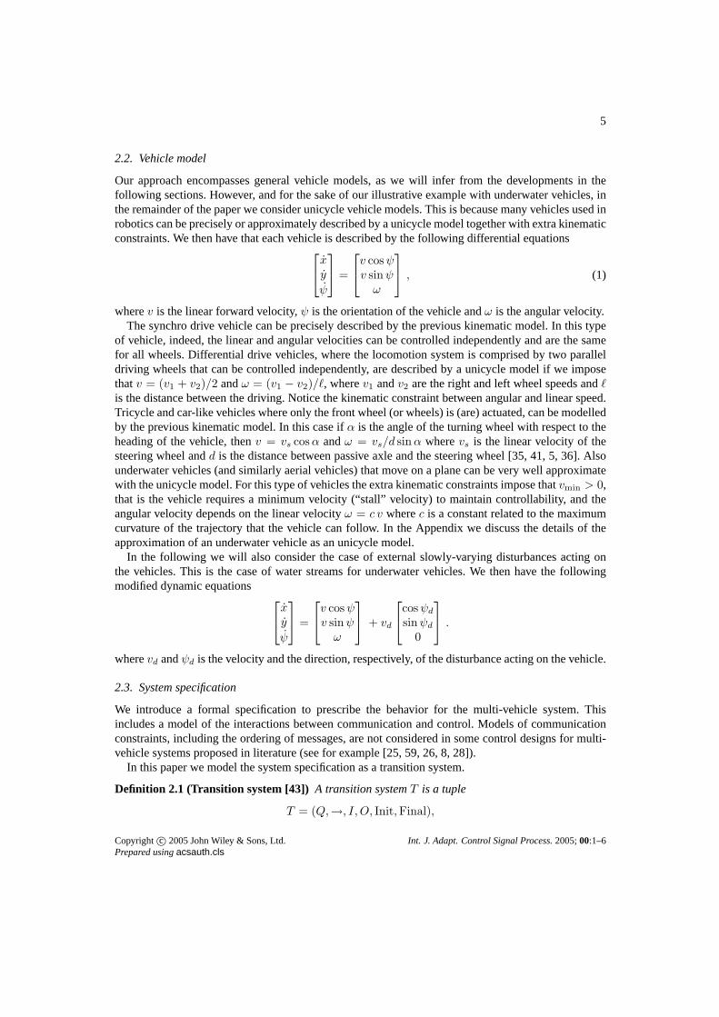
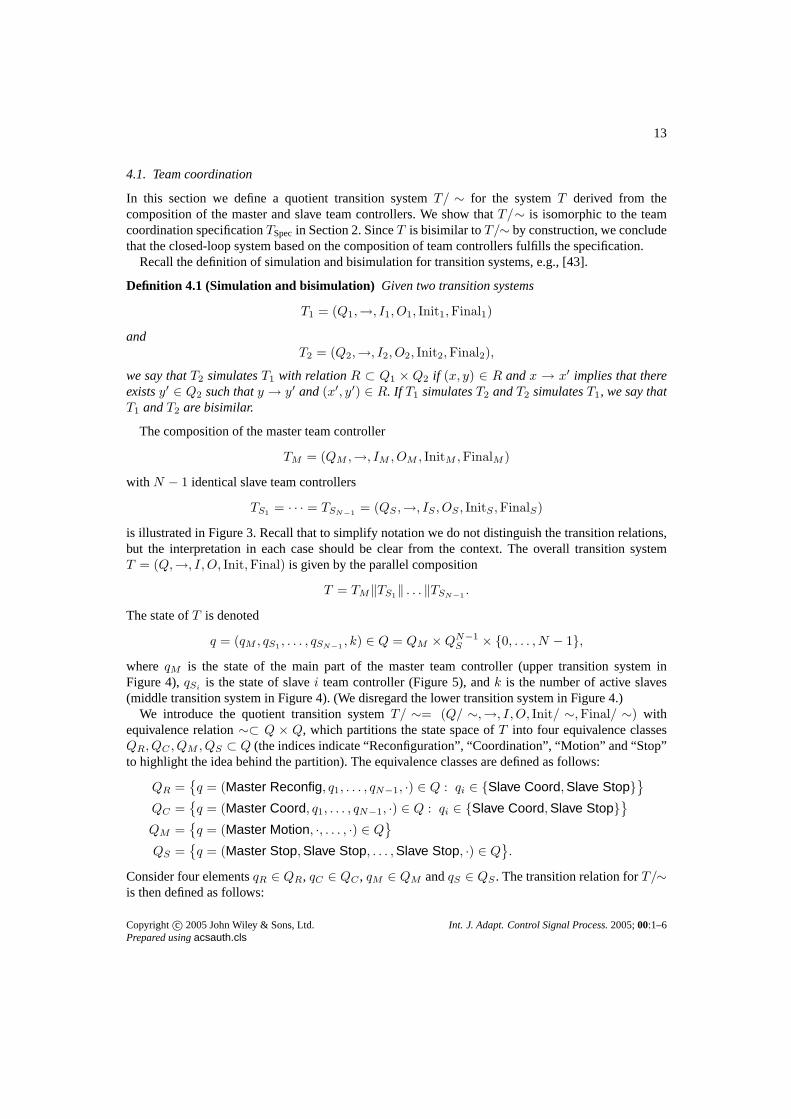
an arc with empty origin representingInit and a vertex with an extra circle representingFinal.The system specification for a coordinated search mission isgiven by the transition system

TSpec= (QSpec,→, ISpec, ∅,Team Coord,Team Stop)

shown in Figure 1. It has four discrete states:Team Coord, Team Reconfig, Team Motion,Team Stop. In a nominal mission the system alternates between two states, Team Coord andTeam Motion, until the mission is completed when a termination condition is satisfied. Note that thissystem specification is fairly general, and captures a wide class of multi-vehicle control problems.

The system starts in theTeam Coord state. A transition toTeam Stop takes place if the terminationcondition is true. Otherwise, inTeam Coord the vehicles exchange their positions and sampleddata prior to the generation of the new waypointsw+ and coordination timest+. The transition toTeam Motion takes place upon the reception ofw+

i . While inTeam Motion, each vehicle is controlledto the designated waypoint within a given coordination timeinterval. The transition toTeam Coordtakes place when all the vehicles reach their designated waypoints. If one vehicle is not able to reachits waypoint within a given coordination time interval a timeout event is generated and the transitionto Team Reconfig is taken. InTeam Reconfig the team executes a reconfiguration operation, whichinvolves a re-allocation of roles. After reconfiguration, the system goes toTeam Coord, where nominal


7

Team Controller

Vehicle Supervisor

Maneuver Controller

(w+, t+) = φ(w, t, e)

x = f(x, u)

(motion commands)e(sample)

exec/stop(maneuver)done/error

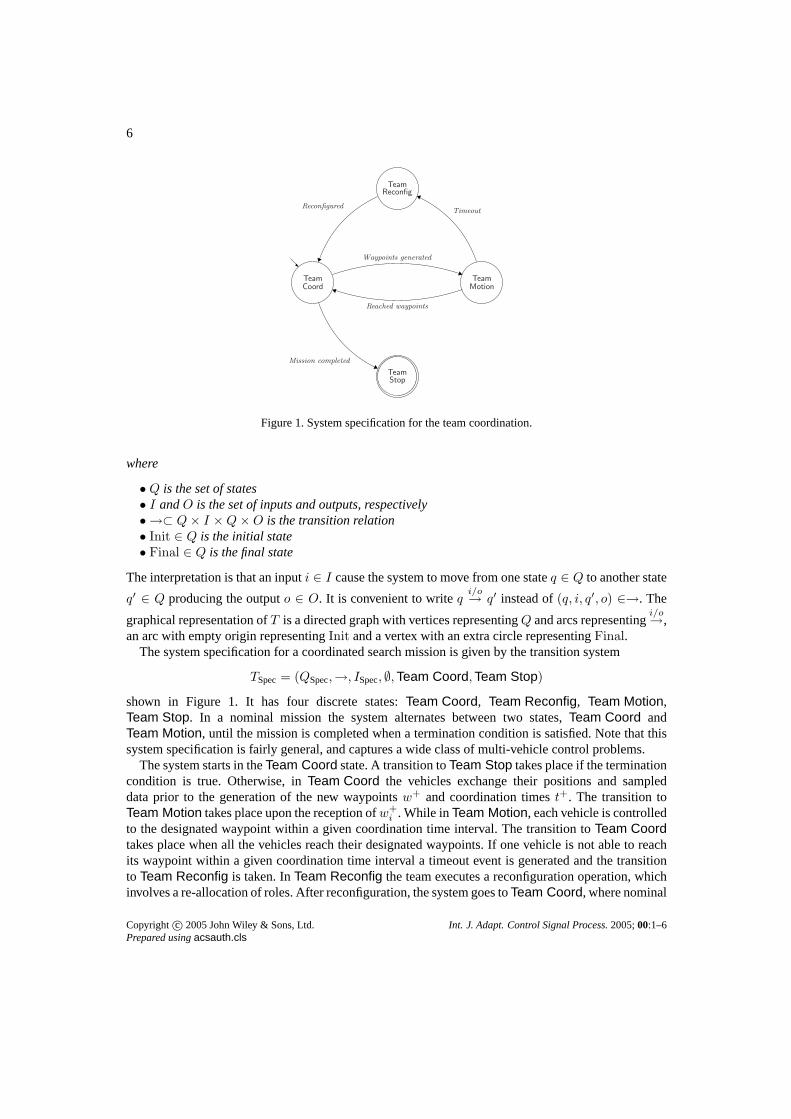
Figure 2. Hierarchical control structure for each vehicle.

execution is resumed for the currently active vehicles. Thetransition toTeam Stop takes place whenthe mission is completed.

In the next section we present our design for the hierarchical control architecture and in Section 4we show that the design fulfills the specification.

3. HIERARCHICAL CONTROL STRUCTURE

3.1. Organization and concepts of operation

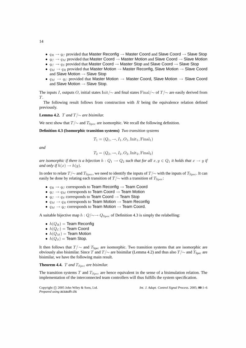
The vehicles inV have the same control structure. Our design for the vehicle control structure isorganized into two pieces: generation of sampling points and execution control. The execution control,in turn, is structured into three layers: team control, vehicle supervision and maneuver control (seeFigure 2). This is an intuitive structure for program developers and system operators.

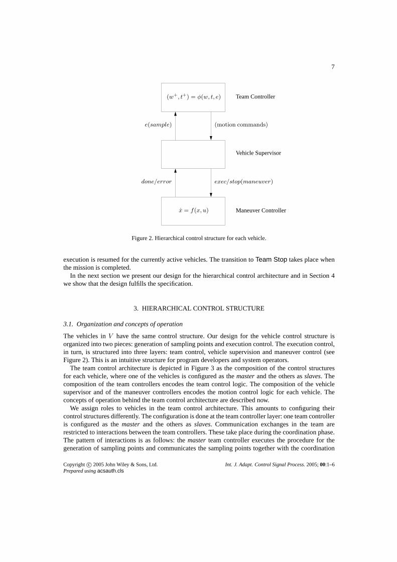
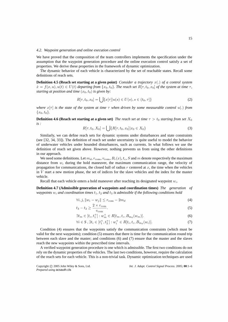
The team control architecture is depicted in Figure 3 as the composition of the control structuresfor each vehicle, where one of the vehicles is configured as the masterand the others asslaves. Thecomposition of the team controllers encodes the team control logic. The composition of the vehiclesupervisor and of the maneuver controllers encodes the motion control logic for each vehicle. Theconcepts of operation behind the team control architectureare described now.

We assign roles to vehicles in the team control architecture. This amounts to configuring theircontrol structures differently. The configuration is done at the team controller layer: one team controlleris configured as themasterand the others asslaves. Communication exchanges in the team arerestricted to interactions between the team controllers. These take place during the coordination phase.The pattern of interactions is as follows: themasterteam controller executes the procedure for thegeneration of sampling points and communicates the sampling points together with the coordination


8

Master

Slave 2 Slave 1

Architecture

Figure 3. Control architecture for a multi-vehicle system with three vehiclesresulting from the composition ofthe control structures for the three vehicles. Arrows between hierarchies represent communication links between

vehicles. Arrows inside each hierarchical stack represent signals between different layers.

times to the other team controllers; upon arrival at the designated sampling point each team controllersends the a message with the sample to themaster; the process starts again when themasterreceivesthe samples from the other team controllers and the termination condition is not true. In this designthere is no need the vehicles to communicate during the time elapsed between the reception of the nextsampling point and the arrival at the sampling point.

From the motion control point of view, each vehicle is abstracted as a provider of prototypicalmaneuvers: different maneuvers may be required for different missions; and the same motions maybe accomplished by different maneuvers. There is one maneuver controller for each type of maneuver.

Consider figure 2 for a description of the motion control logic for each vehicle. The vehiclesupervisor mediates the interactions between the team controller and the maneuver controllers. This isdone for the purpose of modularity; there is a library of maneuvers and of maneuver controllers; and theaddition and deletion of maneuvers to the library does not require changes to the team controller and tothe vehicle supervisor. The vehicle supervisor accepts maneuver commands (or commands to abort thecurrent maneuver) from the team controller and passes the maneuver parameters to the correspondingmaneuver controller for execution, and signals back to the team controller the completion or failure ofthe maneuver. The maneuver controller takes as input a maneuver specification, sends low-level controlcommands to the actuators in continuous time, and signals back to the vehicle supervisor the successor failure of the maneuver.

As we go down in the hierarchy there are certain aspects of thedesign that become more dependenton the dynamics of the vehicles. Thus, in order to explain howwe design maneuvers we considera specific coordination mission, namely the search for the minimum of a scalar field by a team ofunderwater vehicles. In our design this mission uses two types of maneuvers: goto waypoint and hold.The first maneuver drives the vehicle from its current position to the a given waypointwi within agiven coordination time intervalt. The second maneuver keeps the vehicle within a neighborhood of agiven waypoint.


9

3.2. Waypoint generation

As as discussed in Section 2 the way-point generation procedureφ(.) produces the set of samplingpointsw (or way-points in a more general context) and the set of coordination timest = t1, t2, t3.The coordination times are defined as follows:

(i) the mastervehicle is required to arrive at its designated waypoint beforet1 and to stay within agiven range of the waypoint until the end of the communication phase.

(ii) eachslavevehicle is required to arrive at its designated waypoint (where it sends the sample tothemaster) in the time interval[t1, t2] and to stay within a given range of the waypoint until theend of the communication phase.

(iii) the communication phase is required to terminate before t3; each vehicle receives the nextwaypoint from themasterduring the time interval(t2, t3).

This is done to ensure that the vehicles are able to communicate among them during the communicationphase, even in the presence of disturbances.

3.3. Team controller

We model each team controller as a transition system. Since the team controller can be in either masteror slave mode, we have two team controller transition systems. They are described below. The masterteam controller,

TM = (QM ,→, IM , OM , InitM ,FinalM )

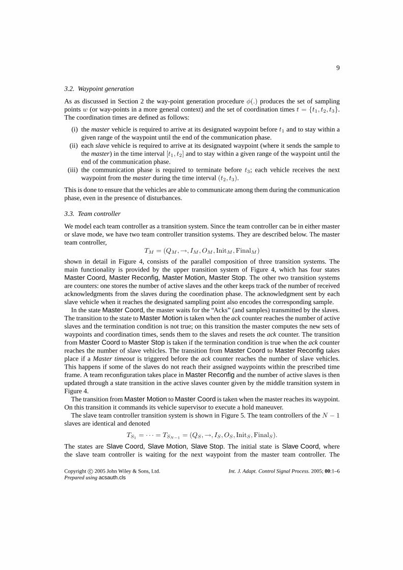
shown in detail in Figure 4, consists of the parallel composition of three transition systems. Themain functionality is provided by the upper transition system of Figure 4, which has four statesMaster Coord, Master Reconfig, Master Motion, Master Stop. The other two transition systemsare counters: one stores the number of active slaves and the other keeps track of the number of receivedacknowledgments from the slaves during the coordination phase. The acknowledgment sent by eachslave vehicle when it reaches the designated sampling pointalso encodes the corresponding sample.

In the stateMaster Coord, the master waits for the “Acks” (and samples) transmitted by the slaves.The transition to the state toMaster Motion is taken when theackcounter reaches the number of activeslaves and the termination condition is not true; on this transition the master computes the new sets ofwaypoints and coordination times, sends them to the slaves and resets theackcounter. The transitionfrom Master Coord to Master Stop is taken if the termination condition is true when theackcounterreaches the number of slave vehicles. The transition fromMaster Coord to Master Reconfig takesplace if aMaster timeoutis triggered before theack counter reaches the number of slave vehicles.This happens if some of the slaves do not reach their assignedwaypoints within the prescribed timeframe. A team reconfiguration takes place inMaster Reconfig and the number of active slaves is thenupdated through a state transition in the active slaves counter given by the middle transition system inFigure 4.

The transition fromMaster Motion to Master Coord is taken when the master reaches its waypoint.On this transition it commands its vehicle supervisor to execute a hold maneuver.

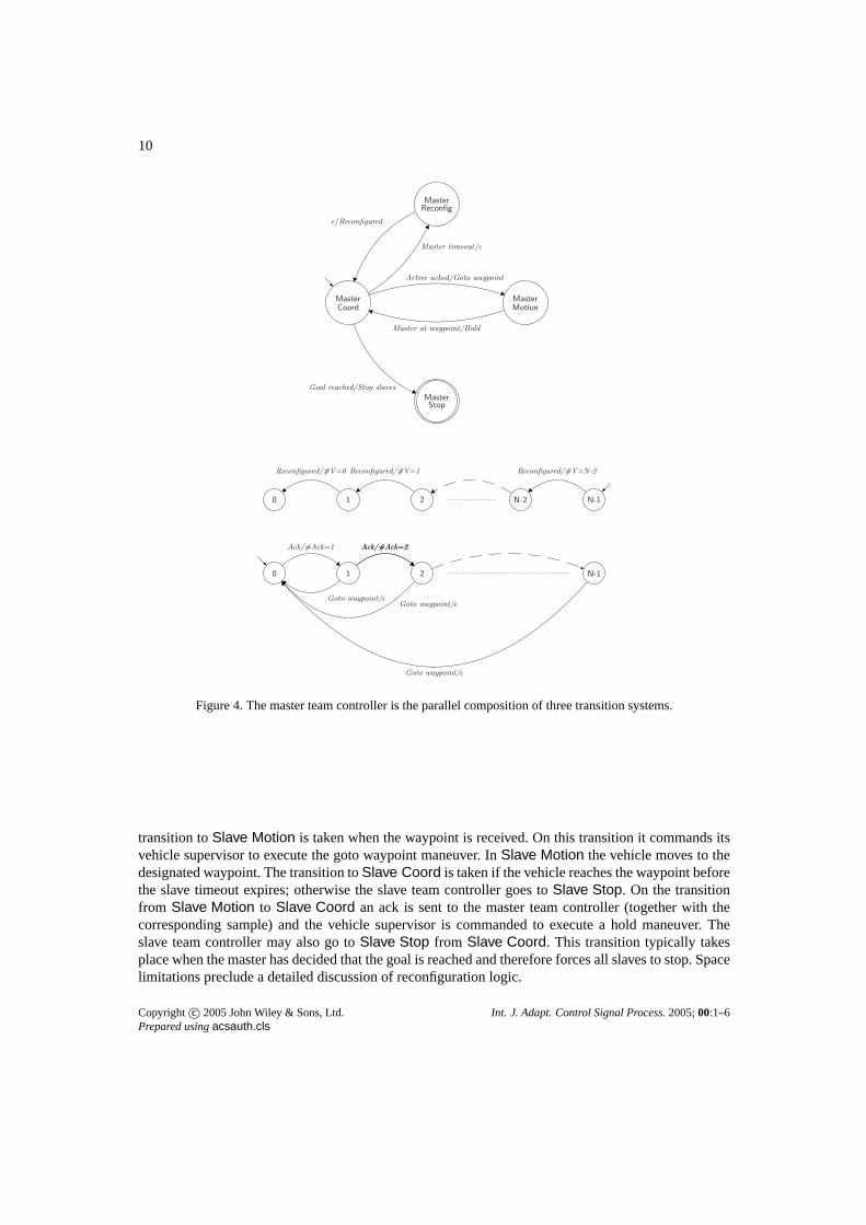
The slave team controller transition system is shown in Figure 5. The team controllers of theN − 1slaves are identical and denoted

TS1= · · · = TSN−1

= (QS ,→, IS , OS , InitS ,FinalS).

The states areSlave Coord, Slave Motion, Slave Stop. The initial state isSlave Coord, wherethe slave team controller is waiting for the next waypoint from the master team controller. The


10

MasterCoord

MasterMotion

MasterReconfig

MasterStop

Active acked/Goto waypoint

Master at waypoint/Hold

Master timeout/ǫ

ǫ/Reconfigured

Goal reached/Stop slaves

0 1 2 N-2 N-1

Reconfigured/#V=1Reconfigured/#V=0 Reconfigured/#V=N-2

0 1 2 N-1

Ack/#Ack=1 Ack/#Ack=2Ack/#Ack=2

Goto waypoint/ǫ

Goto waypoint/ǫGoto waypoint/ǫ

Figure 4. The master team controller is the parallel composition of three transition systems.

transition toSlave Motion is taken when the waypoint is received. On this transition itcommands itsvehicle supervisor to execute the goto waypoint maneuver. In Slave Motion the vehicle moves to thedesignated waypoint. The transition toSlave Coord is taken if the vehicle reaches the waypoint beforethe slave timeout expires; otherwise the slave team controller goes toSlave Stop. On the transitionfrom Slave Motion to Slave Coord an ack is sent to the master team controller (together with thecorresponding sample) and the vehicle supervisor is commanded to execute a hold maneuver. Theslave team controller may also go toSlave Stop from Slave Coord. This transition typically takesplace when the master has decided that the goal is reached andtherefore forces all slaves to stop. Spacelimitations preclude a detailed discussion of reconfiguration logic.


11

SlaveCoord

SlaveMotion

SlaveStop

Goto waypoint/Goto

Slave at waypoint/Ack,Hold

Stop slaves/ǫ

Slave timeout/ǫ

Figure 5. Slave team controller.

Idle

Error

Stop

Motion

goto(ωi, t)/startGoto(ωi, t)

stop/stop

ǫ/Error(code)

stop/stop

doneGoto(sp)/waypoint(sp), startHold(wi, t)

MtimeOut/timeOut

Figure 6. Vehicle supervisor.

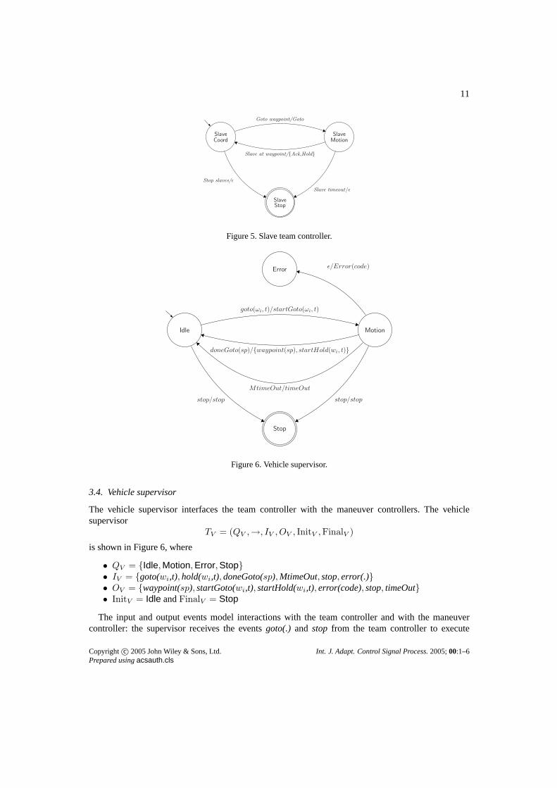
3.4. Vehicle supervisor

The vehicle supervisor interfaces the team controller withthe maneuver controllers. The vehiclesupervisor

TV = (QV ,→, IV , OV , InitV ,FinalV )

is shown in Figure 6, where

• QV = Idle,Motion,Error,Stop• IV = goto(wi,t),hold(wi,t),doneGoto(sp),MtimeOut, stop,error(.)• OV = waypoint(sp), startGoto(wi,t), startHold(wi,t),error(code), stop, timeOut• InitV = Idle andFinalV = Stop

The input and output events model interactions with the teamcontroller and with the maneuvercontroller: the supervisor receives the eventsgoto(.) and stop from the team controller to execute


12

a goto maneuver (with the specified parameters) and to stop the current maneuver respectively; itreceives the eventsdoneGoto(.), error(.) and MTtimeOut from the current maneuver controller toindicate the termination of the current maneuver, the occurrence of an error, or the occurrence of atime out respectively; it sends the eventsstartGoto(.), startHold(.)andstopto start executing a goto ora hold maneuver and to stop the current maneuver; and it sendsthe eventswaypoint(sp), error(code)andtimeOutto the team controller to indicate that the waypoint was reached, that an error of typecodehas occurred and that time out has occurred respectively. Inthe absence of errors, execution alternatesbetween the statesIdle andMotion.

Note that there are no clocks in the vehicle supervisor. The reasons for this are that: (i) both thesupervisor and the maneuver controllers reside on the same vehicle and we can therefore assumereliable communications between them; and (ii) maneuver timeouts are modelled within the maneuvercontrollers.

3.5. Maneuver controller

The aspects of maneuver design are quite dependent on the dynamics of each vehicle. However, andfor the purpose of modularity, maneuver controllers have toconform to a standard interface for theinteractions with the vehicle supervisor. We describe thisinterface now.

The structure of each maneuver controller is as follows

TC = (QC ,→, IC , OC , InitC ,FinalC)

where

• QC = Init,Motion,Error,Stop• IC = start(.), stop• OC = done(.),error(code), stop, timeOut• InitC = Init andFinalC = Stop

In the motion state there is a low-level control law which generates references to actuators incontinuous time. In practice, there may exist states other thanMotion to encode the maneuver controllogic.

4. SYSTEM PROPERTIES

In this section we show how the team control architecture implements the specification. This is donein a modular fashion. First, we show that the high level team coordination implemented through thecomposition of the master and slave team controllers is consistent with the specification under theassumptions that: 1) the generation of waypoints and coordination times produces points reachableboth in space and time; and 2) the online execution control ensures that these points are indeed reached.Second, we state a set of conditions which ensures that the waypoint generation procedure produceswaypoints and coordination times that are reachable both intime and space. Third, we discuss how theonline execution control ensures that the waypoints are indeed reached under the assumption that themaneuver controllers produce guaranteed results. Fourth,we discuss the design of maneuver controllerswhich produce guaranteed results.

This modularity decouples efficiently the behavior of the team from that of the underlyingcoordination algorithm.


13

4.1. Team coordination

In this section we define a quotient transition systemT/ ∼ for the systemT derived from thecomposition of the master and slave team controllers. We show thatT/∼ is isomorphic to the teamcoordination specificationTSpecin Section 2. SinceT is bisimilar toT/∼ by construction, we concludethat the closed-loop system based on the composition of teamcontrollers fulfills the specification.

Recall the definition of simulation and bisimulation for transition systems, e.g., [43].

Definition 4.1 (Simulation and bisimulation) Given two transition systems

T1 = (Q1,→, I1, O1, Init1,Final1)

andT2 = (Q2,→, I2, O2, Init2,Final2),

we say thatT2 simulatesT1 with relationR ⊂ Q1 × Q2 if (x, y) ∈ R andx → x′ implies that thereexistsy′ ∈ Q2 such thaty → y′ and(x′, y′) ∈ R. If T1 simulatesT2 andT2 simulatesT1, we say thatT1 andT2 are bisimilar.

The composition of the master team controller

TM = (QM ,→, IM , OM , InitM ,FinalM )

with N − 1 identical slave team controllers

TS1= · · · = TSN−1

= (QS ,→, IS , OS , InitS ,FinalS)

is illustrated in Figure 3. Recall that to simplify notationwe do not distinguish the transition relations,but the interpretation in each case should be clear from the context. The overall transition systemT = (Q,→, I, O, Init,Final) is given by the parallel composition

T = TM‖TS1‖ . . . ‖TSN−1

.

The state ofT is denoted

q = (qM , qS1, . . . , qSN−1

, k) ∈ Q = QM ×QN−1S × 0, . . . , N − 1,

where qM is the state of the main part of the master team controller (upper transition system inFigure 4),qSi

is the state of slavei team controller (Figure 5), andk is the number of active slaves(middle transition system in Figure 4). (We disregard the lower transition system in Figure 4.)

We introduce the quotient transition systemT/ ∼= (Q/ ∼,→, I, O, Init/ ∼,Final/ ∼) withequivalence relation∼⊂ Q × Q, which partitions the state space ofT into four equivalence classesQR, QC , QM , QS ⊂ Q (the indices indicate “Reconfiguration”, “Coordination”,“Motion” and “Stop”to highlight the idea behind the partition). The equivalence classes are defined as follows:

QR =

q = (Master Reconfig, q1, . . . , qN−1, ·) ∈ Q : qi ∈ Slave Coord,Slave Stop

QC =

q = (Master Coord, q1, . . . , qN−1, ·) ∈ Q : qi ∈ Slave Coord,Slave Stop

QM =

q = (Master Motion, ·, . . . , ·) ∈ Q

QS =

q = (Master Stop,Slave Stop, . . . ,Slave Stop, ·) ∈ Q

.

Consider four elementsqR ∈ QR, qC ∈ QC , qM ∈ QM andqS ∈ QS . The transition relation forT/∼is then defined as follows:


14

• qR → qC provided thatMaster Reconfig → Master Coord andSlave Coord → Slave Stop• qC → qM provided thatMaster Coord → Master Motion andSlave Coord → Slave Motion• qC → qS provided thatMaster Coord → Master Stop andSlave Coord → Slave Stop• qM → qR provided thatMaster Motion → Master Reconfig, Slave Motion → Slave Coord

andSlave Motion → Slave Stop• qM → qC provided thatMaster Motion → Master Coord, Slave Motion → Slave Coord

andSlave Motion → Slave Stop.

The inputsI, outputsO, initial statesInit/∼ and final statesFinal/∼ of T/∼ are easily derived fromT .

The following result follows from construction withR being the equivalence relation definedpreviously.

Lemma 4.2. T andT/∼ are bisimilar.

We next show thatT/∼ andTSpec are isomorphic. We recall the following definition.

Definition 4.3 (Isomorphic transition systems)Two transition systems

T1 = (Q1,→, I1, O1, Init1,Final1)

andT2 = (Q2,→, I2, O2, Init2,Final2)

are isomorphic if there is a bijectionh : Q1 → Q2 such that for allx, y ∈ Q1 it holds thatx → y ifand only ifh(x) → h(y).

In order to relateT/∼ andTSpec, we need to identify the inputs ofT/∼ with the inputs ofTSpec. It caneasily be done by relating each transition ofT/∼ with a transition ofTSpec:

• qR → qC corresponds toTeam Reconfig → Team Coord• qC → qM corresponds toTeam Coord → Team Motion• qC → qS corresponds toTeam Coord → Team Stop• qM → qR corresponds toTeam Motion → Team Reconfig• qM → qC corresponds toTeam Motion → Team Coord.

A suitable bijective maph : Q/∼→ QSpec of Definition 4.3 is simply the relabelling:

• h(QR) = Team Reconfig• h(QC) = Team Coord• h(QM ) = Team Motion• h(QS) = Team Stop.

It then follows thatT/∼ andTSpec are isomorphic. Two transition systems that are isomorphicareobviously also bisimilar. SinceT andT/∼ are bisimilar (Lemma 4.2) and thus alsoT/∼ andTSpecarebisimilar, we have the following main result.

Theorem 4.4. T andTSpec are bisimilar.

The transition systemsT andTSpec are hence equivalent in the sense of a bisimulation relation. Theimplementation of the interconnected team controllers will thus fulfills the system specification.


15

4.2. Waypoint generation and online execution control

We have proved that the composition of the team controllers implements the specification under theassumption that the waypoint generation procedure and the online execution control satisfy a set ofproperties. We derive these properties in the framework of dynamic optimization.

The dynamic behavior of each vehicle is characterized by theset of reachable states. Recall somedefinitions of reach sets.

Definition 4.5 (Reach set starting at a given point)Consider a trajectoryx(.) of a control systemx = f(x, u), u(t) ∈ U(t) departing fromx0, t0. The reach setR[τ, t0, x0] of the system at timeτ ,starting at position and time(x0, t0) is given by:

R[τ, t0, x0] =⋃

x[τ ]|u(s) ∈ U(s), s ∈ (t0, τ ] (2)

wherex[τ ] is the state of the system at timeτ when driven by some measurable controlu(.) fromx0, t0.

Definition 4.6 (Reach set starting at a given set)The reach set at timeτ > t0 starting from setX0

is :R[τ, t0,X0] =

⋃

R[τ, t0, x0]|x0 ∈ X0 (3)

Similarly, we can define reach sets for dynamic systems underdisturbances and state constraints(see [32, 34, 33]). The definition of reach set under uncertainty is quite useful to model the behaviorof underwater vehicles under bounded disturbances, such ascurrents. In what follows we use thedefinition of reach set given above. However, nothing prevents us from using the other definitionsin our approach.

We need some definitions. Letmd, rcom, vcom,Br(x), tc,S andm denote respectively the maximumdistance fromwi during the hold maneuver, the maximum communication range,the velocity ofpropagation for communications, the closed ball of radiusr centered atx, the time when the vehiclesin V start a new motion phase, the set of indices for the slave vehicles and the index for the mastervehicle.

Recall that each vehicle enters a hold maneuver after reaching its designated waypointwi.

Definition 4.7 (Admissible generation of waypoints and coordination times) The generation ofwaypointswi and coordination timest1, t2 andt3 is admissible if the following conditions hold

∀i, j, ‖wi − wj‖ ≤ rcom − 2md (4)

t3 − t2 ≥ 2 × rcomvcom

. (5)

∃tm ∈ [tc, t+1 ] : w+

m ∈ R[tm, tc, Bmd(wm)]. (6)

∀i ∈ S ,∃ti ∈ [t+1 , t+2 ] : w+

i ∈ R[ti, tc, Bmd(wi)]. (7)

Condition (4) ensures that the waypoints satisfy the communication constraints (which must bevalid for the next waypoints); condition (5) ensures that there is time for the communication round tripbetween each slave and the master; and conditions (6) and (7)ensure that the master and the slavesreach the new waypoints within the prescribed time intervals.

A verified waypoint generation procedure is one which is admissible. The first two conditions do notrely on the dynamic properties of the vehicles. The last two conditions, however, require the calculationof the reach sets for each vehicle. This is a non-trivial task. Dynamic optimization techniques are used


16

in [32] for this purpose. The observation is that the reach set is the sub-zero level set of a certain valuefunction. The value function is obtained from the solution of a Hamilton-Jacobi equation. For linearsystems with ellipsoidal constraints duality techniques are used to construct this solution.

The advantage of using value functions for reach set computations is that this approach also enablesus to derive controllers which guarantee that the waypointsare reached. This is in line with the approachproposed in [39, 52].

The reach set formulation enables us to derive maneuver controllers for the hold and goto maneuverswhich ensure guaranteed results. In these maneuvers, we arebasically concerned with controlling thedistance function from the current position of the vehicle to a given waypoint. In this case, we canuse the construction proposed in [31] to calculate the safe set for a one-dimensional pursuit–evasiondifferential game which is easily extended to higher dimensional systems. This construction involvesthe integration of an ordinary differential equation, which describes how the distance evolves with time,and does not require the integration of a Hamilton-Jacobi equation.

5. AUTONOMOUS UNDERWATER VEHICLES IN SEARCH MISSION

In this section we show how to implement a search strategy fora team of autonomous underwatervehicles (AUV) with our control architecture; this basically involves specializing the waypointgeneration procedure and the maneuver design for this search strategy. We also illustrate thesedevelopments with simulation results.

The problem consists of finding the minimum of a temperature field with a search strategy based ona fixed-size version of the simplex optimization algorithm introduced in [49].

The underwater operations pose one additional challenge tothe general search problem for ateam of vehicles. The challenge comes from the nature of underwater communications. Typicallyautonomous underwater vehicles use acoustic communications which are quite constrained in rangeand in bandwidth. This is basically due to the problems associated with the propagation of soundunderwater.

In what follows we consider a team of autonomous underwater vehicles equipped with acousticmodems for communication and some sensing device to measuresome scalar variable, for exampletemperature.

The simplex algorithm is particularly suited for this challenging application. It is quite simple,robust, and very effective in finding the extremum of a scalarfield from few samples. This leads tofeasible requirements for underwater communications.

What also makes this method appealing is the fact that it allows reasoning about vehicle motion indiscrete terms: indeed the simplex algorithm imposes a discretization of the configuration space whichfacilitates the implementation of the proposed hierarchical structure. For example, the conditions forthe generation of admissible waypoints are trivially satisfied with an appropriate choice of the grid size.

For the purpose of clarity we also restrict our search to motions in the horizontal plane.

5.1. Simplex algorithm

The simplex optimization algorithm is a direct search method which behaves much like a gradientdescent method but with no explicit gradient calculation. It is usually applied in situations wherecomputation capability is limited and gradient calculation is difficult, as happens in scalar fieldscorrupted by noise. We are interested in executing a search operation for finding the minimum of a


17

d

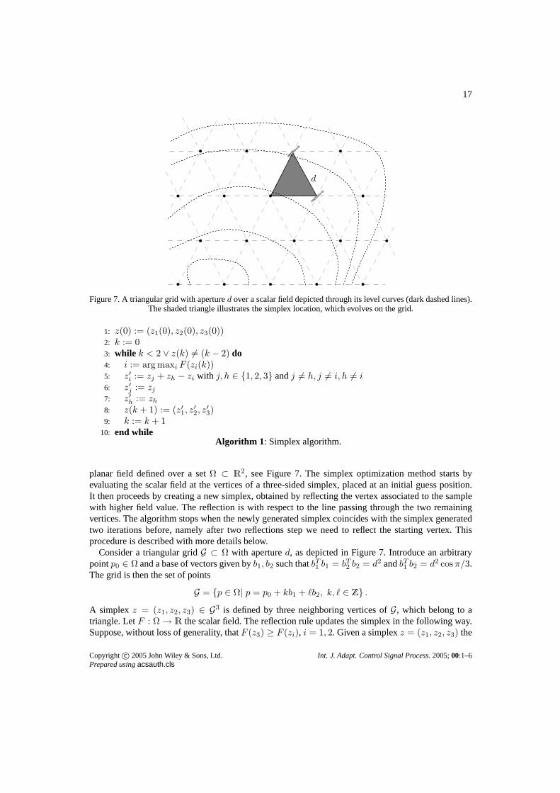
Figure 7. A triangular grid with apertured over a scalar field depicted through its level curves (dark dashed lines).The shaded triangle illustrates the simplex location, which evolves on the grid.

1: z(0) := (z1(0), z2(0), z3(0))2: k := 03: while k < 2 ∨ z(k) 6= (k − 2) do4: i := arg maxi F (zi(k))5: z′i := zj + zh − zi with j, h ∈ 1, 2, 3 andj 6= h, j 6= i, h 6= i6: z′j := zj

7: z′h := zh

8: z(k + 1) := (z′1, z′

2, z′

3)9: k := k + 1

10: end whileAlgorithm 1 : Simplex algorithm.

planar field defined over a setΩ ⊂ R2, see Figure 7. The simplex optimization method starts by

evaluating the scalar field at the vertices of a three-sided simplex, placed at an initial guess position.It then proceeds by creating a new simplex, obtained by reflecting the vertex associated to the samplewith higher field value. The reflection is with respect to the line passing through the two remainingvertices. The algorithm stops when the newly generated simplex coincides with the simplex generatedtwo iterations before, namely after two reflections step we need to reflect the starting vertex. Thisprocedure is described with more details below.

Consider a triangular gridG ⊂ Ω with apertured, as depicted in Figure 7. Introduce an arbitrarypointp0 ∈ Ω and a base of vectors given byb1, b2 such thatbT1 b1 = bT2 b2 = d2 andbT1 b2 = d2 cosπ/3.The grid is then the set of points

G = p ∈ Ω| p = p0 + kb1 + ℓb2, k, ℓ ∈ Z .A simplex z = (z1, z2, z3) ∈ G3 is defined by three neighboring vertices ofG, which belong to atriangle. LetF : Ω → R the scalar field. The reflection rule updates the simplex in the following way.Suppose, without loss of generality, thatF (z3) ≥ F (zi), i = 1, 2. Given a simplexz = (z1, z2, z3) the


18

wjwk

wi

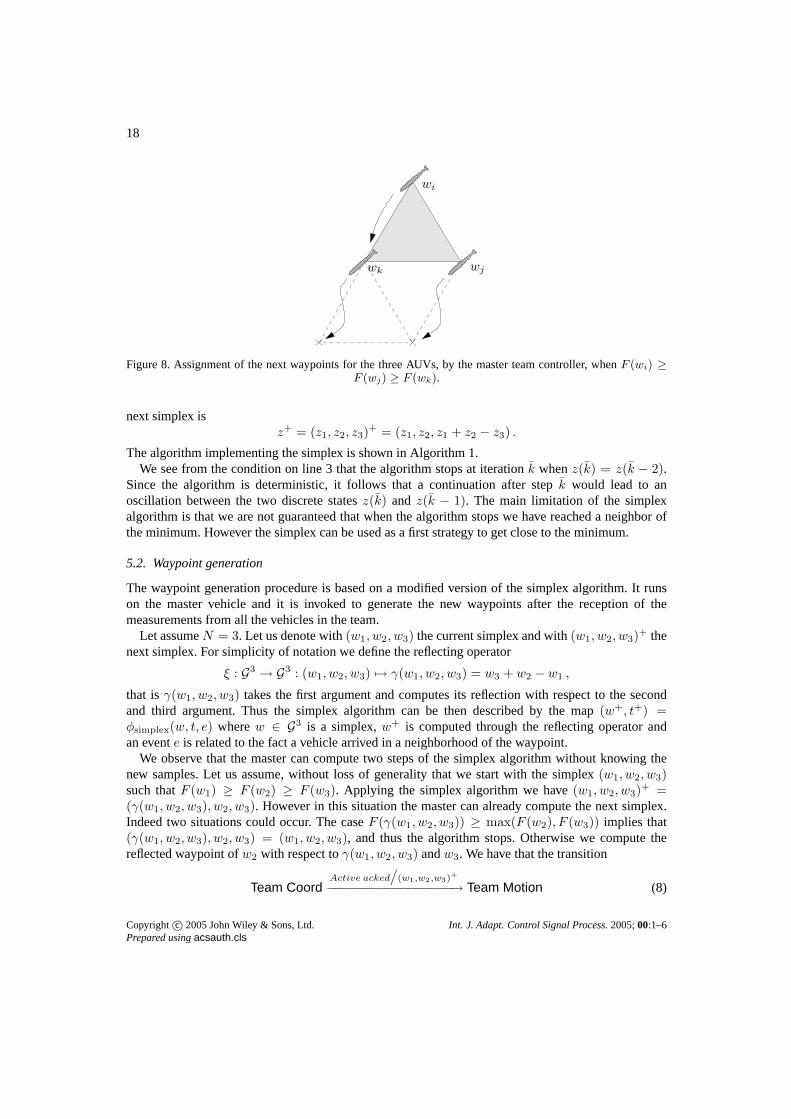
Figure 8. Assignment of the next waypoints for the three AUVs, by the master team controller, whenF (wi) ≥F (wj) ≥ F (wk).

next simplex isz+ = (z1, z2, z3)

+ = (z1, z2, z1 + z2 − z3) .

The algorithm implementing the simplex is shown in Algorithm 1.We see from the condition on line 3 that the algorithm stops atiterationk whenz(k) = z(k − 2).

Since the algorithm is deterministic, it follows that a continuation after stepk would lead to anoscillation between the two discrete statesz(k) and z(k − 1). The main limitation of the simplexalgorithm is that we are not guaranteed that when the algorithm stops we have reached a neighbor ofthe minimum. However the simplex can be used as a first strategy to get close to the minimum.

5.2. Waypoint generation

The waypoint generation procedure is based on a modified version of the simplex algorithm. It runson the master vehicle and it is invoked to generate the new waypoints after the reception of themeasurements from all the vehicles in the team.

Let assumeN = 3. Let us denote with(w1, w2, w3) the current simplex and with(w1, w2, w3)+ the

next simplex. For simplicity of notation we define the reflecting operator

ξ : G3 → G3 : (w1, w2, w3) 7→ γ(w1, w2, w3) = w3 + w2 − w1 ,

that isγ(w1, w2, w3) takes the first argument and computes its reflection with respect to the secondand third argument. Thus the simplex algorithm can be then described by the map(w+, t+) =φsimplex(w, t, e) wherew ∈ G3 is a simplex,w+ is computed through the reflecting operator andan evente is related to the fact a vehicle arrived in a neighborhood of the waypoint.

We observe that the master can compute two steps of the simplex algorithm without knowing thenew samples. Let us assume, without loss of generality that we start with the simplex(w1, w2, w3)such thatF (w1) ≥ F (w2) ≥ F (w3). Applying the simplex algorithm we have(w1, w2, w3)

+ =(γ(w1, w2, w3), w2, w3). However in this situation the master can already compute the next simplex.Indeed two situations could occur. The caseF (γ(w1, w2, w3)) ≥ max(F (w2), F (w3)) implies that(γ(w1, w2, w3), w2, w3) = (w1, w2, w3), and thus the algorithm stops. Otherwise we compute thereflected waypoint ofw2 with respect toγ(w1, w2, w3) andw3. We have that the transition

Team CoordActive acked

/

(w1,w2,w3)+

−−−−−−−−−−−−−−−−−→ Team Motion (8)


19

Master

Master

MasterSlave

Slave

Slave

(a) (b) (c)

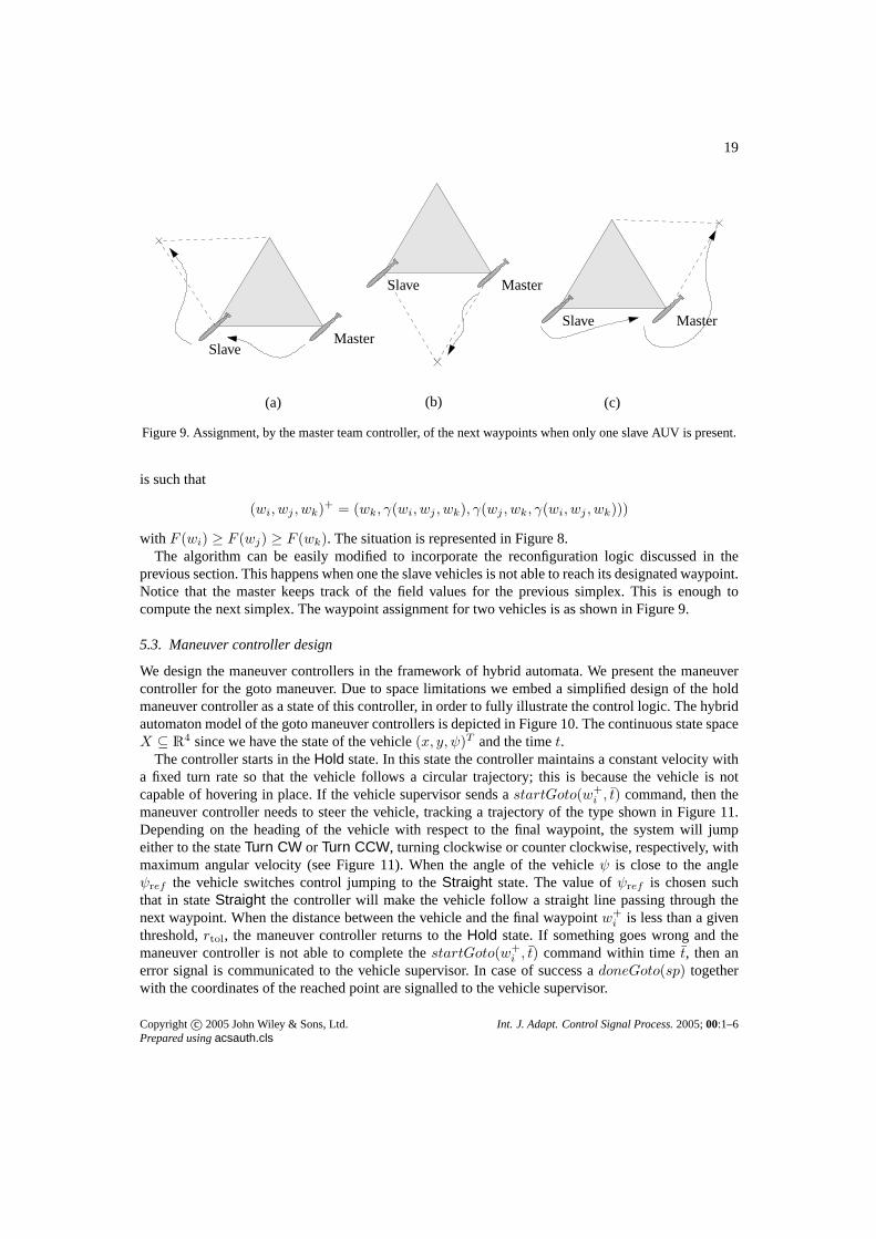
Figure 9. Assignment, by the master team controller, of the next waypointswhen only one slave AUV is present.

is such that

(wi, wj , wk)+ = (wk, γ(wi, wj , wk), γ(wj , wk, γ(wi, wj , wk)))

with F (wi) ≥ F (wj) ≥ F (wk). The situation is represented in Figure 8.The algorithm can be easily modified to incorporate the reconfiguration logic discussed in the

previous section. This happens when one the slave vehicles is not able to reach its designated waypoint.Notice that the master keeps track of the field values for the previous simplex. This is enough tocompute the next simplex. The waypoint assignment for two vehicles is as shown in Figure 9.

5.3. Maneuver controller design

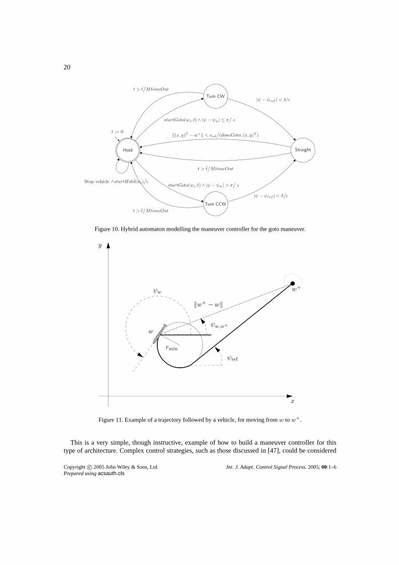
We design the maneuver controllers in the framework of hybrid automata. We present the maneuvercontroller for the goto maneuver. Due to space limitations we embed a simplified design of the holdmaneuver controller as a state of this controller, in order to fully illustrate the control logic. The hybridautomaton model of the goto maneuver controllers is depicted in Figure 10. The continuous state spaceX ⊆ R

4 since we have the state of the vehicle(x, y, ψ)T and the timet.The controller starts in theHold state. In this state the controller maintains a constant velocity with

a fixed turn rate so that the vehicle follows a circular trajectory; this is because the vehicle is notcapable of hovering in place. If the vehicle supervisor sends astartGoto(w+

i , t) command, then themaneuver controller needs to steer the vehicle, tracking a trajectory of the type shown in Figure 11.Depending on the heading of the vehicle with respect to the final waypoint, the system will jumpeither to the stateTurn CW or Turn CCW, turning clockwise or counter clockwise, respectively, withmaximum angular velocity (see Figure 11). When the angle of the vehicleψ is close to the angleψref the vehicle switches control jumping to theStraight state. The value ofψref is chosen suchthat in stateStraight the controller will make the vehicle follow a straight line passing through thenext waypoint. When the distance between the vehicle and the final waypointw+

i is less than a giventhreshold,rtol, the maneuver controller returns to theHold state. If something goes wrong and themaneuver controller is not able to complete thestartGoto(w+

i , t) command within timet, then anerror signal is communicated to the vehicle supervisor. In case of success adoneGoto(sp) togetherwith the coordinates of the reached point are signalled to the vehicle supervisor.


20

Hold

t := 0

Stop vehicle ∧startHold(wi)/

ǫ

Straight

Turn CW

Turn CCW

startGoto(wi, t) ∧ |ψ − ψw| ≤ π/

ǫ

startGoto(wi, t) ∧ |ψ − ψw| > π/

ǫ

‖(x, y)T − w+‖ < rtol/

(doneGoto, (x, y)T )

t > t/

MtimeOut

|ψ − ψref | < δ/ǫ

|ψ − ψref | < δ/

ǫ

t > t/

MtimeOut

t > t/

MtimeOut

Figure 10. Hybrid automaton modelling the maneuver controller for the gotomaneuver.

x

y

‖w+ − w‖

ψw

ψw,w+

ψref

rmin

w

w+

Figure 11. Example of a trajectory followed by a vehicle, for moving fromw tow+.

This is a very simple, though instructive, example of how to build a maneuver controller for thistype of architecture. Complex control strategies, such as those discussed in [47], could be considered


21

−100 −50 0 50 100 150−50

0

50

100

(a) AUVs’ trajectories after the first iteration.

−100 −50 0 50 100 150−50

0

50

100

(b) Situation after 70 seconds.

−100 −50 0 50 100 150−50

0

50

100

(c) Situation after 100 seconds.

−100 −50 0 50 100 150−50

0

50

100

(d) Search mission completed after 135 seconds.

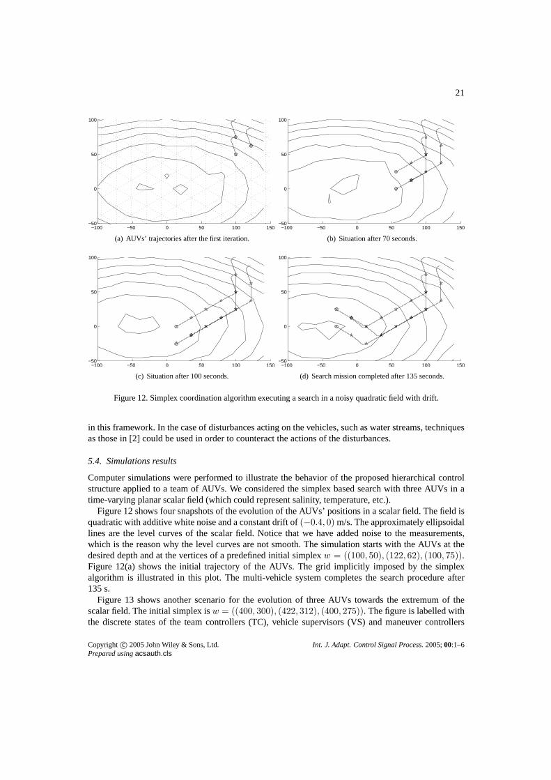
Figure 12. Simplex coordination algorithm executing a search in a noisy quadratic field with drift.

in this framework. In the case of disturbances acting on the vehicles, such as water streams, techniquesas those in [2] could be used in order to counteract the actions of the disturbances.

5.4. Simulations results

Computer simulations were performed to illustrate the behavior of the proposed hierarchical controlstructure applied to a team of AUVs. We considered the simplex based search with three AUVs in atime-varying planar scalar field (which could represent salinity, temperature, etc.).

Figure 12 shows four snapshots of the evolution of the AUVs’ positions in a scalar field. The field isquadratic with additive white noise and a constant drift of(−0.4, 0) m/s. The approximately ellipsoidallines are the level curves of the scalar field. Notice that we have added noise to the measurements,which is the reason why the level curves are not smooth. The simulation starts with the AUVs at thedesired depth and at the vertices of a predefined initial simplex w = ((100, 50), (122, 62), (100, 75)).Figure 12(a) shows the initial trajectory of the AUVs. The grid implicitly imposed by the simplexalgorithm is illustrated in this plot. The multi-vehicle system completes the search procedure after135 s.

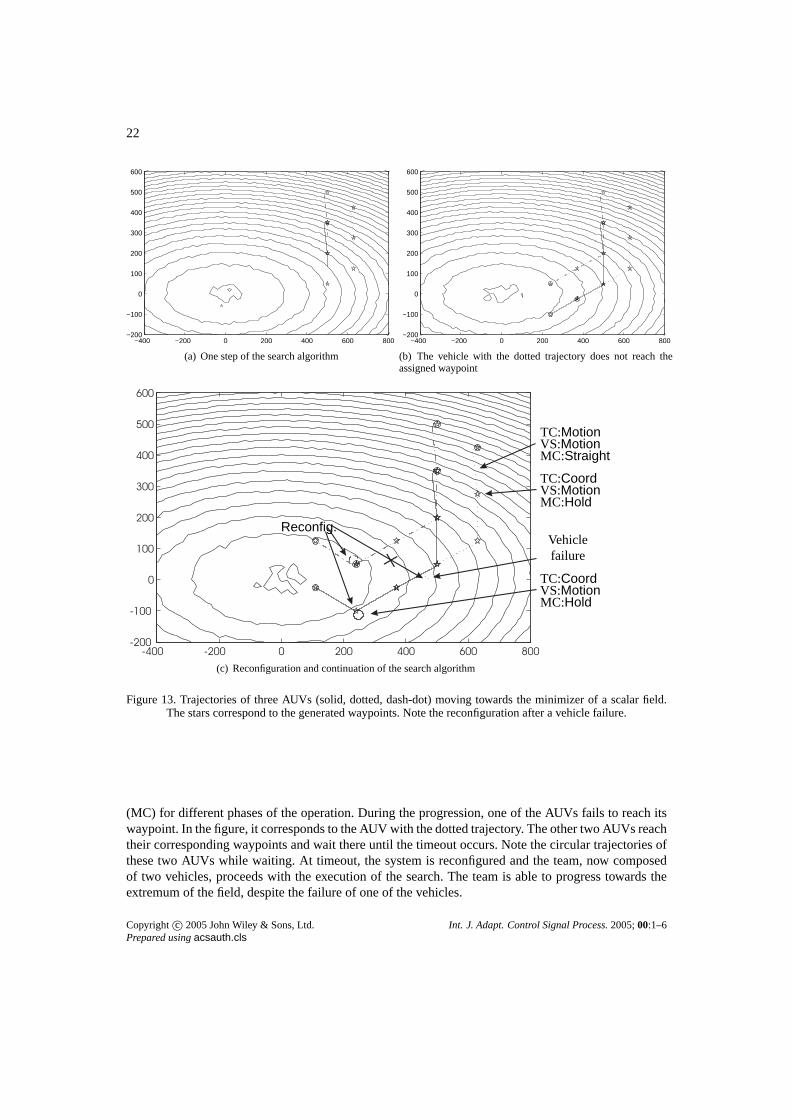
Figure 13 shows another scenario for the evolution of three AUVs towards the extremum of thescalar field. The initial simplex isw = ((400, 300), (422, 312), (400, 275)). The figure is labelled withthe discrete states of the team controllers (TC), vehicle supervisors (VS) and maneuver controllers


22

−400 −200 0 200 400 600 800−200

−100

0

100

200

300

400

500

600

(a) One step of the search algorithm

−400 −200 0 200 400 600 800−200

−100

0

100

200

300

400

500

600

(b) The vehicle with the dotted trajectory does not reach theassigned waypoint

+

Reconfig.Vehiclefailure

TC:MotionVS:MotionMC:Straight

TC:CoordVS:MotionMC:Hold

TC:CoordVS:MotionMC:Hold

(c) Reconfiguration and continuation of the search algorithm

Figure 13. Trajectories of three AUVs (solid, dotted, dash-dot) moving towards the minimizer of a scalar field.The stars correspond to the generated waypoints. Note the reconfiguration after a vehicle failure.

(MC) for different phases of the operation. During the progression, one of the AUVs fails to reach itswaypoint. In the figure, it corresponds to the AUV with the dotted trajectory. The other two AUVs reachtheir corresponding waypoints and wait there until the timeout occurs. Note the circular trajectories ofthese two AUVs while waiting. At timeout, the system is reconfigured and the team, now composedof two vehicles, proceeds with the execution of the search. The team is able to progress towards theextremum of the field, despite the failure of one of the vehicles.


23

6. CONCLUSIONS

We presented a design of a hierarchical control architecture for coordinated multi-vehicle operations.The design space is large and heterogeneous. We structure the space by first decomposing it intowaypoint generation and online execution control. The waypoint generation procedure generates thewaypoints for the team to search for the minimum of a scalar field under dynamic and communicationconstraints and in accordance to a given optimization algorithm. Execution control is organized as athree level hierarchy of team controller, supervisor, and maneuver controller.

It is shown that the controller implementation is consistent with the system specification on thedesired team behavior. This is done in a modular fashion by layering the execution control anddesigning each layer to ensure that the controllers produceguaranteed results under the assumptionthat the controllers at the adjacent layers also produce guaranteed results.

Computer simulations illustrate the overall system performance for a multi-vehicle search missionwhich is motivated by the classical simplex optimization algorithm. This example illustrates thespecialization of the design to a specific application. Basically this involves specializing the waypointgeneration procedure according to the coordination strategy and the maneuver controllers according tothe specific dynamics of each vehicle.

REFERENCES

1. S. Spry A. Girard and J. K. Hedrick. Real-time embedded hybrid control software for intelligent cruise control applications.IEEE Robotics and Automation Magazine – Special Issue on ITS, 12(1):22–28, 2005.

2. M. Aicardi, G. Casalino, G. Indiveri, A. Aguiar, P. Encarnacao, and A. Pascoal. A planar path following controller forunderactuated marine vehicles. InProc. 9th Mediterranean Conference on Control and Automation, 2001.

3. R. Bachmayer and N. E. Leonard. Vehicle networks for gradient descent in a sampled environment. InProceedings ofIEEE Conference on Decision and Control, pages 112–117, 2002.

4. S. Bayraktar, G. Fainekos, and G. J. Pappas. Experimental cooperative control of unmanned aerial vehicles. InProceedingsIEEE Conference Decision and Control. IEEE Control Society, 2004.

5. R. W. Beard, T. W. McLain, M. Goodrich, and E. P. Anderson. Coordinated target assignment and intercept for unmannedair vehicles.IEEE Transactions on Robotics and Automation, 18(6):911–922, 2002.

6. E. Burian, D. Yoerger, A. Bradley, and H. Singh. Gradient search with autonomous underwater vehicles using scalarmeasurements. InIEEE Symp. Autonomous Underwater Vehicle Technology, pages 86–89, 1996.

7. D. Van Cleave. Trends and technologies for uninhabited autonomous vehicles. In T. Samad and G. Balas, editors,Software-Enabled Control: Information Technology for Dynamical Systems. IEEE Press/John Wiley and Sons, 2002.

8. J. Cortes, S. Martınez, and F. Bullo. Robust rendezvous for mobile autonomous agents via proximity graphs in arbitrarydimensions.IEEE Transaction on Automatic Control, 2004. To appear.

9. D. E. Culler and H. Mulder. Smart sensors to network the world. Scientific American, 2004.10. T. Curtin, J. Bellingham, J. Catipovic, and D. Webb. Autonomous ocean sampling networks.Oceanography, 6(3):86–94,

1993.11. T. Curtin and J. G. Bellingham. Guest editorial: Autonomous ocean-sampling networks.IEEE Journal of Oceanic

Engineering, 26(4):423, 2001.12. R. D’Andrea. Robot soccer: a platform for systems engineering. Computers in Education Journal, 10(1):57–61, 2000.13. R. D’Andrea and R. Murray. The roboflag competition. InProceedings of the American Controls Conference, pages

650–655. IEEE, 2003.14. J. Borges de Sousa, A. Girard, and K. Hedrick. Real-time hybrid control of mobile offshore base scaled models. In

Proceedings of the American Control Conference, 2000.15. J. Borges de Sousa, K. H. Johansson, A. Speranzon, and J. Silva. A control architecture for multiple submarines in

coordinated search missions. InProceedings of IFAC World Congress, 2005.16. J. Borges de Sousa and F. Lobo Pereira. A generalized vehicle-based control architecture for multiple auvs. InProceedings

of the OCEANS ’95 MTS/IEEE, pages 1643–50. IEEE, 1995.17. J. Borges de Sousa, T. Simsek, and P. Varaiya. Task planning and execution for uav teams. InProceedings of the IEEE

Conference on Decision and Control. IEEE, 2004.


24

18. G. Fainekos, H. Kress-Gazit, and G. Pappas. Hybrid controllers for path planning : a temporal logic approach. InProceedings IEEE Conference Decision and Control. IEEE Control Society, 2005.

19. E. Fiorelli, P. Bhatta, and N. E. Leonard. Adaptive sampling using feedback control of an autonomous underwater gliderfleet. InProc. 13th Int. Symp. on Unmanned Untethered Submersible Technology (UUST). IEEE, 2003.

20. T. I. Fossen.Guidance and Control of Ocean Vehicles. John Wiley and Sons Ltd., 1994.21. A. Girard, J. B. Sousa, and K. Hedrick. An overview of emerging results in networked multi-vehicle systems. In

Proceedings of the Decision and Control Conference, Orlando, USA, 2001.22. D. N. Godbole, J. Lygeros, and S. Sastry. Hierarchical hybrid control: An ivhs case study. In A. Nerode P. Antsaklis and

S. Sastry, editors,Hybrid Systems II, LNCS, pages 166–90. Birkhauser, 1995.23. Gwyn Griffiths, editor.Technology and applications of Autonomous Underwater Vehicles. Ocean Science and Technology

Volume 2. Taylor & Francis Group, 2003.24. J. K. Hedrick, M. Tomizuka, and P. Varaiya. Control issuesin automated highway systems.IEEE Control Systems

Magazine, 14(6):21–32, 1994.25. J. P. Hespanha, H. J. Kim, and S. Sastry. Multiple-agent probabilistic pursuit–evasion games. InIEEE Conference on

Decision and Control, volume 3, pages 2432–2437, 1999.26. A. Jadbabaie, J. Lin, and A. S. Morse. Coordination of groups of mobile autonomous agents using nearest neighbor rules.

IEEE Transactions on Automatic Control, 48(6):988–1001, 2003.27. J. Jang and C. Tomlin. Autopilot design for the stanford dragonfly uav: Validation through hardware-in-the-loop

simulation. InProceedings of the AIAA Guidance, Navigation, and Control Conference. AAIAA, 2001.28. K. H. Johansson, A. Speranzon, and S. Zampieri. On quantization and communication topologies in multi-vehicle

rendezvous. InProceedings of IFAC World Congress, 2005.29. L. C. Kendall, D. K. Costello, H. Warrior, L. C. Langebrake, W. Hou, J. T. Patten, and E. Kaltenbacher. Ocean-science

mission needs: Real-time auv data for command, control and model inputs. IEEE Journal of Oceanic Engineering,26(4):742–751, 2001.

30. D. B. Kilfoyle and A. B. Baggeroer. The state of the art in underwater acoustic telemetry.IEEE Journal of OceanicEngineering, 25(1):4–27, 2000.

31. N. N. Krasovskii and A. I. Subbotin.Game-theoretical control problems. Springer-Verlag, 1988.32. A. B. Kurzhanskii and P. Varaiya. Dynamic optimization forreachability problems.Journal of Optimization Theory &

Applications, 108(2):227–51, 2001.33. A. B. Kurzhanskii and P. Varaiya. On reachability under uncertainty. Siam Journal of Control and Optimization,

41(1):181–216, 2002.34. A. B. Kurzhanskii and P. Varaiya. Optimization methods fortarget problems of control. InProceedings of Mathematical

Theory of Networks and Systems Conference, 2002.35. J.-P. Laumond, S. Sekhavat, and F. Lamiraux.Guidelines in Nonholonomic Motion Planning for Mobile Robots, volume

299, chapter 1. Lectures Notes in Control and Information Sciences, 1998.36. S. M. LaValle. Planning Algorithms. Cambridge University Press, 2006. Also available at

http://msl.cs.uiuc.edu/planning/.37. E. Lewis, editor.Principles of Naval Architecture. Society of Naval Architects and Marine Engineers, 1989. 2nd revision.38. P. Lima and G. N. Saridis.Design of Intelligent Control Systems Based on Hierarchical Stochastic Automata. Intelligent

Control and Intelligent Automation. World Scientific Publisher Co., 1996.39. J. Lygeros, Datta N. Godbole, and Shankar Sastry. A game theoretic approach to hybrid system design. Technical Report

UCB/ERL M95/77, University of California, Berkeley. Electronics Research Laboratory, 1995.40. M. Mazo, A. Speranzon, K. H. Johansson, and X. Hu. Multi-robot tracking of a moving object using directional sensors.

In Proceedings of the International Conference on Robotics and Automation (ICRA), 2004.41. G. Oriolo, A. Luca, and M. Vendittelli. Wmr control via dynamic feedback linearization: Design.IEEE Transactions on

Control Systems Technology, 2002.42. T. J. Prestero. Verification of a six-degree of freedom simulation model for the remus auv. Master’s thesis, Massachusetts

Institute of Technology / Woods Hole Oceanographic Institution, Departments of Ocean and Mechanical Engineering,2001.

43. A. Puri and P. Varaiya. Decidable hybrid systems.Computer and Mathematical Modeling, 11(23):191–202, 1996.44. G. Remmers, R. Taylor, P. Palo, and R. Brackett. Mobile offshore base: A seabasing option. InProceedings of Third

International Workshop on Very Large Floating Structures, pages 1–7, 1999.45. G. N. Saridis and K. P. Valavanis. Analytical design of intelligent machines.Automatic, 24(2):123–33, 1988.46. J. Silva, A. Speranzon, J. B. de Sousa, and K. H. Johansson. Hierarchical search strategy for a team of autonomousvehicles.

In Proceedings of the 2004 IAV conference. IFAC, 2004.47. P. Soueres, A. Balluchi, and A. Bicchi. Optimal feedback control for line tracking with a bounded-curvature vehicle.

International Journal of Control, 74(10):1009–1019, 2001.48. E. M. Sozer, M. Stojanovic, and J. G. Proakis. Underwateracoustic networks.IEEE Journal of Oceanic Engineering,

25(1):72–83, 2000.49. W. Spendley, G.R. Hext, and F.R. Himsworth. Sequential applications of simplex designs in optimization and evolutionary

operation.Technometrics, 4:441–461, 1962.


25

50. J. Sprinkle, J. Eklund, and S. Sastry. Deciding to land a uav safely in real time. InProceedings of American ControlConference, pages 8–10. AAIAA, 2005.

51. Roger Stokey, Ben Allen, Tom Austin, Rob Goldsborough, Ned Forrester, Mike Purcell, and Chris von Alt. Enablingtechnologies for remus docking: An integral component of an autonomous ocean-sampling network.IEEE Journal ofOceanic Engineering, 26(4):487–497, 2001.

52. C. J. Tomlin, J. Lygeros, and S. Shankar Sastry. A game theoretic approach to controller design for hybrid systems.Proceedings of the IEEE, 88(7):949–70, 2000.

53. P. Varaiya. Smart cars on smart roads: problems of control.IEEE Transactions on Automatic Control, 38(3):195–207,February 1993.

54. P. Varaiya. Towards a layered view of control. InProceedings of the 36th IEEE Conference on Decision and Control,pages 1187–90. IEEE, 1997.

55. P. Varaiya. Reach set computation using optimal control. In Proceedings of the KIT Workshop on Verification of HybridSystems. Verimag, Grenoble, France, 1998.

56. P. Varaiya. A question about hierarchical systems. Personal communication, November 1999.57. P. Varaiya and S. E. Shladover. Sketch of an ivhs systems architecture. InProceedings of the VNIS ’91. Vehicle Navigation

and Information Systems Conference, pages 909–922. IEEE, 1991.58. M. Veloso. Autonomous robot soccer teams.The Bridge, National Academy of Engineering, 33(1):8–12, 2003.59. R. Vidal, O. Shakernia, J. Kim, D. Shim, and S. Sastry. Probabilistic pursuit-evasion games: Theory, implementation and

experimental evaluation.IEEE Transactions on Robotics and Automation, 8(5):662–669, 2002.60. J. Scott Willcox, James G. Bellingham, Yanwu Zhang, and Arthur B. Baggeroer. Performance metrics for oceanographic

surveys with autonomous underwater vehicles.IEEE Journal of Oceanic Engineering, 26(4):711–725, 2001.

APPENDIX

Underwater Vehicle Model

This section discusses the mapping of a nonlinear model of underwater vehicles to the kinematicmodel described on Section 2.2. Autonomous underwater vehicles (AUV’s) are best described asnonlinear systems (see [20] for details). Two coordinate frames are considered: body-fixed and earth-fixed. In what follows, the notation from the Society of NavalArchitects and Marine Engineers(SNAME) [37] is used. The motions in the body-fixed frame are described by 6 velocity componentsv = (v1, v2) = [u, v, w, p, q, r] respectively, surge, sway, heave, roll, pitch, and yaw, relative to aconstant velocity coordinate frame moving with the ocean current. The six components of position andattitude in the earth-fixed frame areη = (η1, η2) = [x, y, z, φ, θ, ψ]. The earth-fixed reference framecan be considered inertial for the AUV.

The velocities in both reference frames are related throughthe Euler angle transformation

η = J(η2)v (9)

or

x = u cosψ cos θ + v(cosψ sin θ sinφ− sinψ cosφ) + w(sinψ sinφ+ cosψ cosφ sin θ)

y = u sinψ cos θ + v(cosψ cosφ+ sinφ sin θ sinψ) + w(sin θ sinψ cosφ− cosψ sinφ)

z = −u sin θ + v cos θ sinψ + w cos θ cosφ

θ = p+ q sinφ tan θ + r cosφ tan θ

φ = q cosφ− r sinφ

ψ = qsinφ

cos θ+ r

cosφ

cos θ, θ 6= ±90


26

φ

θ

ψxb

yb

zb

X

Y

Z

u (surge)

p (roll)w (heave)

r (yaw)

v (sway)q (pitch)

(x, y, z)

(a) (b)

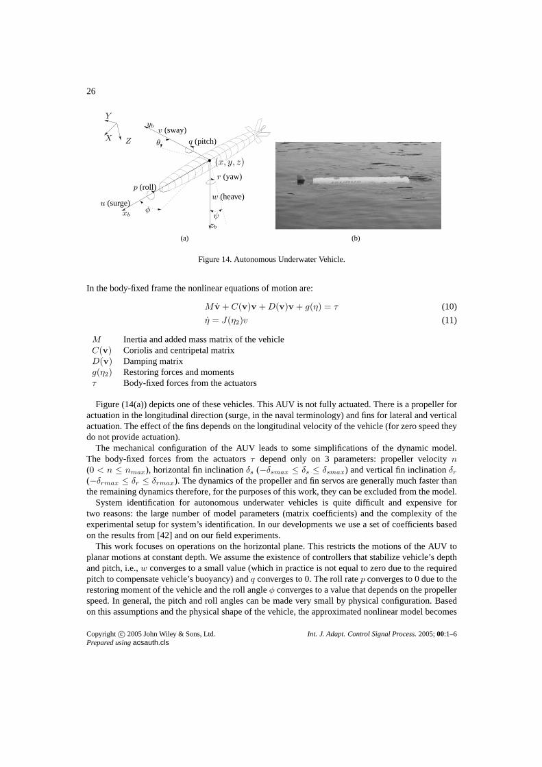
Figure 14. Autonomous Underwater Vehicle.

In the body-fixed frame the nonlinear equations of motion are:

M v + C(v)v +D(v)v + g(η) = τ (10)

η = J(η2)v (11)

M Inertia and added mass matrix of the vehicleC(v) Coriolis and centripetal matrixD(v) Damping matrixg(η2) Restoring forces and momentsτ Body-fixed forces from the actuators

Figure (14(a)) depicts one of these vehicles. This AUV is notfully actuated. There is a propeller foractuation in the longitudinal direction (surge, in the naval terminology) and fins for lateral and verticalactuation. The effect of the fins depends on the longitudinalvelocity of the vehicle (for zero speed theydo not provide actuation).

The mechanical configuration of the AUV leads to some simplifications of the dynamic model.The body-fixed forces from the actuatorsτ depend only on 3 parameters: propeller velocityn(0 < n ≤ nmax), horizontal fin inclinationδs (−δsmax ≤ δs ≤ δsmax) and vertical fin inclinationδr(−δrmax ≤ δr ≤ δrmax). The dynamics of the propeller and fin servos are generally much faster thanthe remaining dynamics therefore, for the purposes of this work, they can be excluded from the model.

System identification for autonomous underwater vehicles is quite difficult and expensive fortwo reasons: the large number of model parameters (matrix coefficients) and the complexity of theexperimental setup for system’s identification. In our developments we use a set of coefficients basedon the results from [42] and on our field experiments.

This work focuses on operations on the horizontal plane. This restricts the motions of the AUV toplanar motions at constant depth. We assume the existence ofcontrollers that stabilize vehicle’s depthand pitch, i.e.,w converges to a small value (which in practice is not equal to zero due to the requiredpitch to compensate vehicle’s buoyancy) andq converges to 0. The roll ratep converges to 0 due to therestoring moment of the vehicle and the roll angleφ converges to a value that depends on the propellerspeed. In general, the pitch and roll angles can be made very small by physical configuration. Basedon this assumptions and the physical shape of the vehicle, the approximated nonlinear model becomes


27

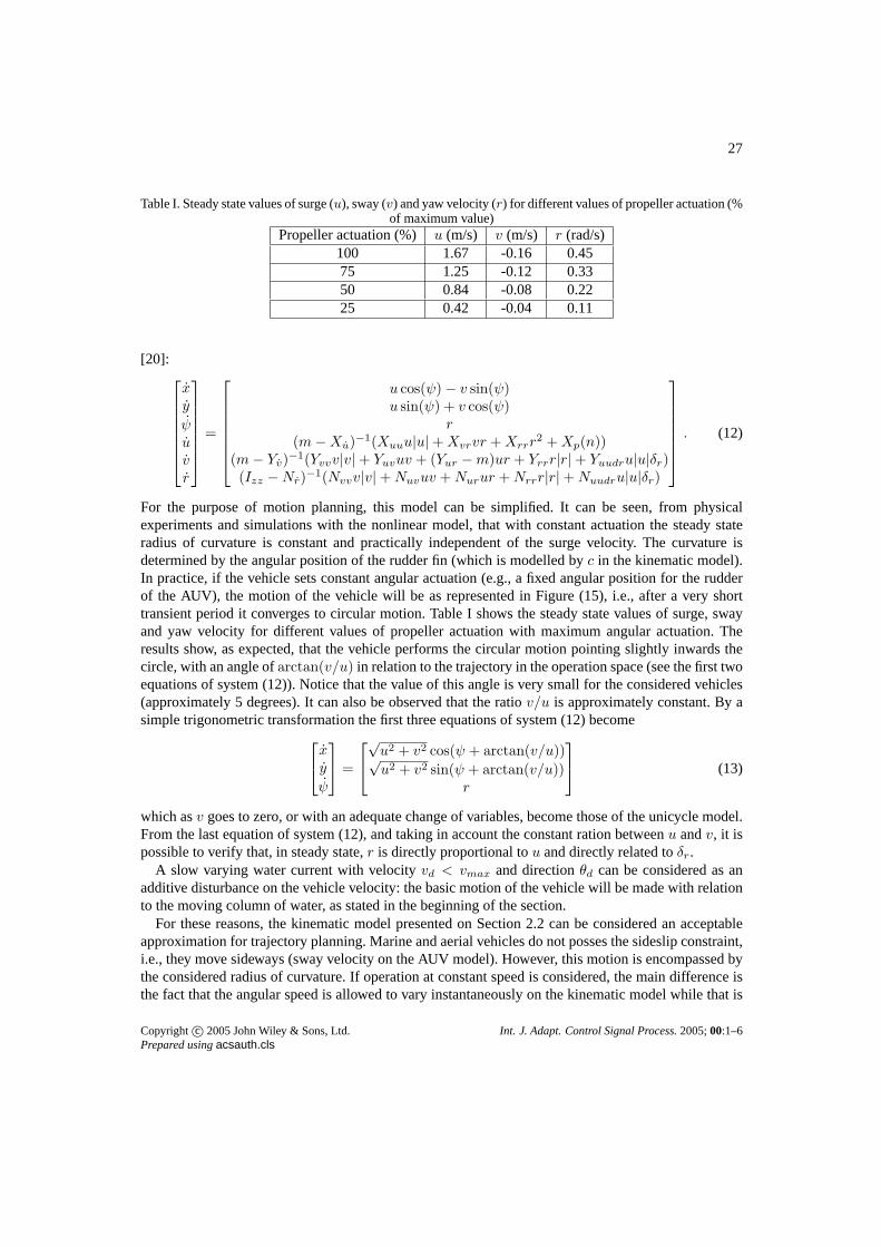
Table I. Steady state values of surge (u), sway (v) and yaw velocity (r) for different values of propeller actuation (%of maximum value)

Propeller actuation (%) u (m/s) v (m/s) r (rad/s)100 1.67 -0.16 0.4575 1.25 -0.12 0.3350 0.84 -0.08 0.2225 0.42 -0.04 0.11

[20]:

xy

ψuvr

=

u cos(ψ) − v sin(ψ)u sin(ψ) + v cos(ψ)

r(m−Xu)−1(Xuuu|u| +Xvrvr +Xrrr

2 +Xp(n))(m− Yv)−1(Yvvv|v| + Yuvuv + (Yur −m)ur + Yrrr|r| + Yuudru|u|δr)(Izz −Nr)

−1(Nvvv|v| +Nuvuv +Nurur +Nrrr|r| +Nuudru|u|δr)

. (12)

For the purpose of motion planning, this model can be simplified. It can be seen, from physicalexperiments and simulations with the nonlinear model, thatwith constant actuation the steady stateradius of curvature is constant and practically independent of the surge velocity. The curvature isdetermined by the angular position of the rudder fin (which ismodelled byc in the kinematic model).In practice, if the vehicle sets constant angular actuation(e.g., a fixed angular position for the rudderof the AUV), the motion of the vehicle will be as represented in Figure (15), i.e., after a very shorttransient period it converges to circular motion. Table I shows the steady state values of surge, swayand yaw velocity for different values of propeller actuation with maximum angular actuation. Theresults show, as expected, that the vehicle performs the circular motion pointing slightly inwards thecircle, with an angle ofarctan(v/u) in relation to the trajectory in the operation space (see thefirst twoequations of system (12)). Notice that the value of this angle is very small for the considered vehicles(approximately 5 degrees). It can also be observed that the ratio v/u is approximately constant. By asimple trigonometric transformation the first three equations of system (12) become

xy

ψ

=

√u2 + v2 cos(ψ + arctan(v/u))√u2 + v2 sin(ψ + arctan(v/u))

r

(13)

which asv goes to zero, or with an adequate change of variables, becomethose of the unicycle model.From the last equation of system (12), and taking in account the constant ration betweenu andv, it ispossible to verify that, in steady state,r is directly proportional tou and directly related toδr.

A slow varying water current with velocityvd < vmax and directionθd can be considered as anadditive disturbance on the vehicle velocity: the basic motion of the vehicle will be made with relationto the moving column of water, as stated in the beginning of the section.

For these reasons, the kinematic model presented on Section2.2 can be considered an acceptableapproximation for trajectory planning. Marine and aerial vehicles do not posses the sideslip constraint,i.e., they move sideways (sway velocity on the AUV model). However, this motion is encompassed bythe considered radius of curvature. If operation at constant speed is considered, the main difference isthe fact that the angular speed is allowed to vary instantaneously on the kinematic model while that is


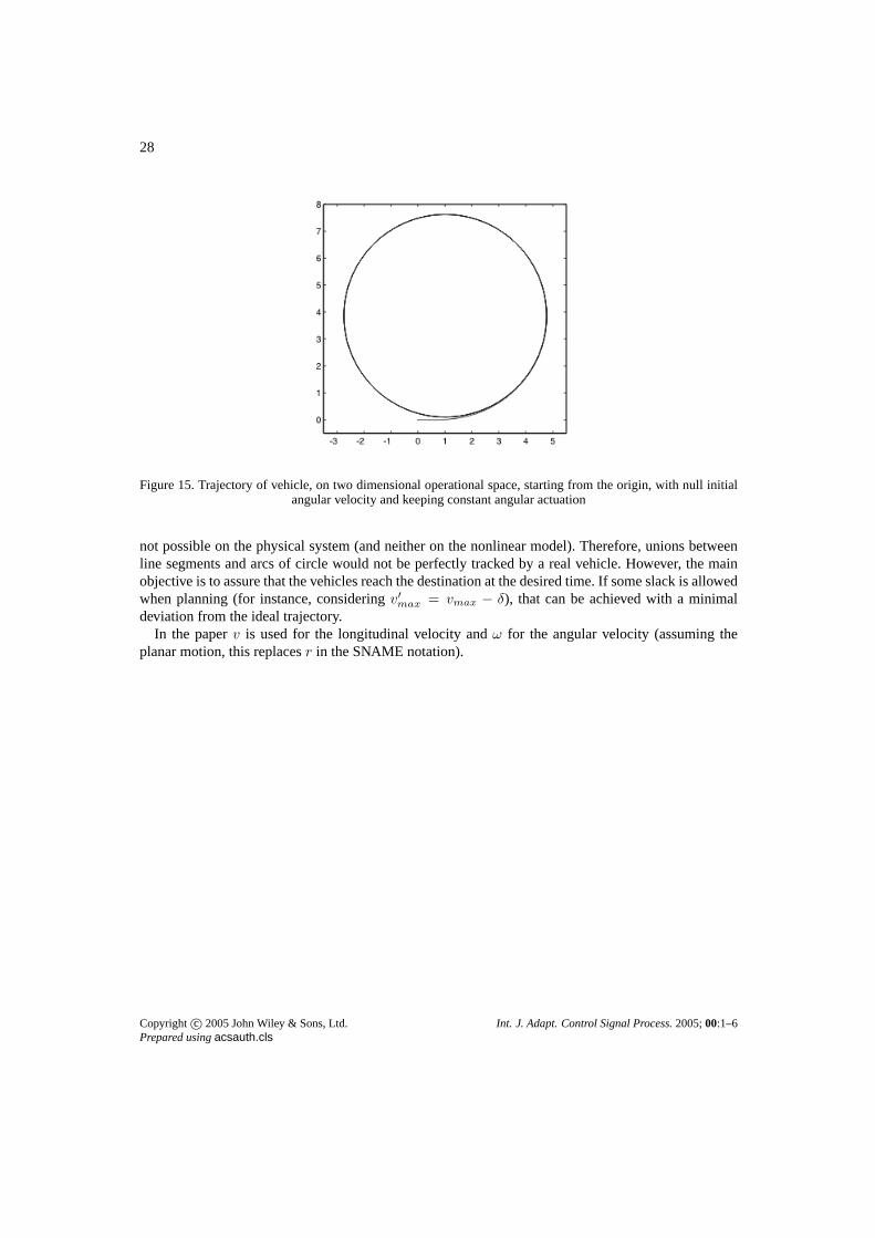
28

Figure 15. Trajectory of vehicle, on two dimensional operational space, starting from the origin, with null initialangular velocity and keeping constant angular actuation

not possible on the physical system (and neither on the nonlinear model). Therefore, unions betweenline segments and arcs of circle would not be perfectly tracked by a real vehicle. However, the mainobjective is to assure that the vehicles reach the destination at the desired time. If some slack is allowedwhen planning (for instance, consideringv′max = vmax − δ), that can be achieved with a minimaldeviation from the ideal trajectory.

In the paperv is used for the longitudinal velocity andω for the angular velocity (assuming theplanar motion, this replacesr in the SNAME notation).


a verified hierarchical control architecture for coordinated multi

Documents