a visual interactive method for prime implicants
TRANSCRIPT
A VISUAL INTERACTIVE METHOD FOR PRIME IMPLICANTS
IDENTIFICATION
Francesco Di Maio1, Samuele Baronchelli1, Enrico Zio1,2
1 Energy Department, Politecnico di Milano
Via Ponzio 34/3, 20133 Milano, Italy
2 Chair on System Science and Energetic Challenge
European Foundation for New Energy – Electricite de France
Ecole Centrale, Paris, and Supelec, Paris, France
ABSTRACT
We propose a visual interactive method for the identification of the Prime Implicants (PIs) of dynamic non-
coherent systems. Visual interactive methods integrate mathematical and symbolic models with runtime
interaction and real-time graphic display, which allow visualizing the underlying physical relationships
among process parameters. The proposed method is based on a parallel coordinates data mining tool that
relies on an innovative pruning procedure which, on the basis of a proper selection of characteristic features
of the accident sequences, retrieves the PIs among the whole set of Implicants in terms of process
parameters values and/or components failure states. The method is exemplified on an artificial case study
and, then, applied for the dynamic reliability analysis of the Airlock System (AS) of a CANDU reactor.
1. INTRODUCTION
Dynamic reliability methods aim at complementing the capability of traditional static approaches
(e.g. Event Trees (ETs) and Fault Trees (FTs)) by accounting for the system dynamic behavior and
its interactions with the system state transition process [Devooght, 1992; Aldemir et al., 2008; Zio
et al., 2009; Di Maio et al., 2011a]. An important task to be accomplished by dynamic reliability
methods is the identification of Prime Implicants (PIs), which extend the traditional concept of
minimal cut sets (mcs) for systems with dynamic interactions among physical parameters of the
process, stochastic discrete failure events and hardware/software/human errors [Aldemir et al.,
2013]: PIs are, thus, defined as the minimal sets of process parameters values and/or components
failure states that are sufficient to cause a failure (top event) of a dynamic system. The logic behind
these systems is that failed and working states of the same components can both lead the system to
failure, i.e., systems have a non-coherent structure function. As an example, a system composed by
components A, B and C for which a PI that causes a system failure is , ,A B C (components A and B
failed, and component C working) is a non-coherent system. Traditionally, non-coherent structure
functions have been interpreted as indication of poor system design. On the other hand, in [Beeson,
2002] it has been shown that an effective prioritization of maintenance actions can be done only by
PIs identification of non-coherent structure functions. With respect to the previous example: if
components A, B and C have failed, C should be the last component to be repaired in order to avoid
system failure. Furthermore, PIs identification allows taking additional counteracting measures to
prevent system failure, for example by forcing failure of component C when component A and B
have already failed [Sharvia et al., 2008].
In the circumstance of non-coherent structure functions, traditional methods, e.g. based on mcs
analysis, cannot be applied for the identification of PIs [Zio et al., 2009]. Analytical methods
[Quine, 1952; McCluskey, 1956] and graphical methods [Karnaugh, 1953] have been introduced,
even if the actual implementation of these methods becomes very time-consuming when the number
of variables in the structure function is large [Sen, 1993] and when the failure dependencies render
the problem combinatorial [Di Maio et al., 2013a]. The issue is one of completeness, i.e., one
situation is when one has on hand an incomplete set of implicants from which he/she wants to
identify the subset of PIs (which will also be incomplete); another is when one wants to identify a
complete set of PIs. This latter situation is the one that has been daunting researchers and is here
addressed. Dynamic Flowgraph Methodology (DFM) provides a modeling and analysis
environment in which the system variables are represented by a finite number of states and the
system dynamics is expressed by cause-and-effect relationships among these states. DFM is based
on parameter values discretization and can produce “timed FTs”, which are FTs in which timing
relations among failure events are systematically taken into account [Yau et al., 1998; Guarro et al.,
2012]. Then, based on an optimized modification of the analytical method initially developed by
Quine and McCluskey [Quine, 1952; McCluskey, 1956], DFM yields “time stamped” PIs by
deductive/inductive analysis aimed at determining how the system reaches a certain failure state.
Another approach resorts to the formulation of the PIs identification problem as a covering
problem, i.e., the problem of covering a complete set of implicants by a given subset of PIs. In this
form, the problem has been solved by transforming it into an optimization problem, where we look,
resorting to evolutionary algorithms, such as Genetic Algorithm (GA) [Sen, 1993] and Differential
Evolution (DE) [Di Maio et al., 2013b], for the minimum combination of implicants that can
guarantee the best coverage of all the process parameters values and/or components failure states
that make the system fail. These techniques have proven very effective, with significant
computational savings, but often remain “black boxes” as to the interpretation of the physical
relationships among process variables and component failure occurrences.
In this work, a visual interactive method is proposed to overcome this latter limitation and increase
the confidence in the provided PIs: interactions make users feel “participants rather than spectators”
[Hurrion, 1980] and grasp complex and extensive information on the system behavior at the same
time [Schramm et al., 2007], so that the decision making task can be facilitated [Wagner et al.,
1996].
According to the degree of interaction between the user and the model, three classes of interaction
and visualization can be described: post-processing, tracking and steering [Bell et al., 1986;
Marshall et al., 1990]. Post-processing methods do not allow the user to observe intermediate
results during the simulation and she/he has no control over the process parameters that are driven
by a third phenomenological model; output data are stored in a database and later retrieved for
being treated. Tracking methods offer intermediate observations of the results and the user may
follow the simulation by means of various visualization tools (e.g., multiple windows, charts
animations). Finally, steering methods allow the user to interact with the system model during
simulation, following the changes generated in the results [Wagner et al., 1996].
In this work, we aim at developing a visual interactive post-processing method for treating a large
number of accident sequences for retrieving (mining) the PIs of a dynamic system. Historically, one
of the first visual data mining techniques being introduced is the grand tour [Buja et al., 1985;
Wegman, 2003], which is an animation of the data and whose basic idea is to look at a data cloud
from all possible points of view; another useful technique for the visualization of high-dimensional
and multivariate datasets on a two-dimensional plot is the parallel coordinates diagram [Inselberg,
1985], which is in many senses a generalization of a two-dimensional cartesian plot: parallel
coordinates are based on nodes which are on the parallel axis and on edges, which are those
polylines linking the nodes on two neighboring axes [Zhou et al., 2008]. However, the
representation of massive amount of data can lead to a considerable overplotting and it can be
misleading for the analysts [Wegman et al., 1997].
To tackle this problem in the context of PIs identification, in this paper we innovatively propose to
implement an automatic pruning procedure of a parallel coordinates diagram that can be used for
visualizing the accident sequences of a system and for reducing the whole set of Implicants into PIs.
The key aspect of the automatic pruning procedure consists into the identification of a proper
feature of the accident sequences that is directly related to the characteristics of “minimal sets of
process parameters values and/or components failure states that are sufficient to cause a failure (top
event) of a dynamic system”, i.e., the PI. This feature is the literal cost of the implicant (i.e., the
number of components whose behavior is specified in the accident sequence). This technique can be
seen as if implemented on a touch screen, where the analyst can interact with the model in order to
prioritize the accident sequences according to their importance with respect to the system end state
of interest, at the same time easily interpreting the relationships among the process parameters.
The paper is organized as follows. In Section 2, the rationale behind literal cost is introduced as key
feature for an effective implementation of a visual interactive method used for PIs identification. In
Section 3, the artificial case study is presented, highlighting its non-coherence. In Section 4, the
case study of the CANDU AS is shown. In Section 5, the proposed technique is applied to the case
studies of Sections 2 and 3, and the results discussed. Conclusions and remarks are given in Section
6.
2. THE METHOD
In this work, we propose a novel method for PIs identification of a dynamic non-coherent system
that aims at guaranteeing interpretability of the representation and of the results, with a controlled
computational burden with respect to other dynamic reliability methods. The method is based on an
innovative pre-selection of the feature that characterizes the accident sequences to be analyzed, in
order to retieve (mine) within the whole set of implicants, those sequences that are PIs of the
dynamic system under analysis. In particular, our method can be resumed into four successive steps,
namely:
1. Feature selection: this step marks the difference with other methods implemented for PI
identification (e.g., analytical methods [Quine, 1952; McCluskey, 1956], graphical methods
[Karnaugh, 1953], DFM [Yau et al., 1998; Guarro et al., 2012], Meta-products Binary
Decision Diagrams (BDDs) [Coudert et al., 1992; Rauzy et al, 1997] or consensus BDDs
[[Beeson, 2002]: the component state is not the only information used for retrieving
(mining) from the set of Implicants the whole set of PIs, but insightful features of the
accident sequences can also be considered variables, such as continuous process variables,
(i.e., temperature and pressure) or stochastic discrete variables (i.e., timing of component
failure events and the number of components whose behavior is specified in the accident
sequence). For our aim, since PIs are the minimal combination of process parameters values
and/or components failure states among the whole list of conditions that bring the system
into failure, we innovatively select the timing of components failures and the literal cost
(i.e., the number of components whose behavior is specified in the accident sequence) as the
most important features for PIs identification according to a parsimony principle: PIs are
indeed those combinations with as few as possible values and events that are capable of
leading the system into a failure state [Rocco et al., 2004].
2. Simulation of accident sequences: depending on the problem at hand, a suitable simulation
tool for the accident evolution simulation is run (e.g., a thermal hydraulic code, a
computational fluid dynamics code, a structural analysis code, a finite elements code, etc.)
to collect the values of the optimally selected features of Step 1 for all possible accident
sequences, and identify all the combinations of process variables values and events which
lead to the failure mode under analysis (implicants); among these, PIs have to be searched.
3. Representation of the accident sequences: visualization of the accident sequences leading to
the failure mode of interest is done by a parallel coordinates diagram. The idea of the
parallel coordinates is to sacrifice the orthogonal axis in order to obtain a planar diagram,
where each accident sequence is represented by a polyline that connects nodes on adjacent
parallel axes. In agreement with the feature selection step, if the considered system is made
up by n components, then the first n parallel coordinates represent the states of the n
components, while the n+1th axis corresponds to the literal cost of the simulated accident
sequences. Note that, concerning the first n coordinates, if the components are Boolean they
can assume only two possible states (e.g. working/failed at a specific time instant);
otherwise, if the components can be found in different states of functioning or can fail at
different times, it is necessary to resort to a multistate description. In our case, the different
value levels of the multistate variables indicate the different time instants at which the
components fail. In particular, with respect to a generic component X, the multistate variable
can assume four different values:
- @ 0X t , if X fails at t=0 (“early failure”)
- @ 2X t , if X fails at t=2 (“intermediate failure”)
- @ 5X t , if X fails at t=5 (“late failure”)
- X , if X does not fail
The concepts of PI can be applied to multistate components as well, provided that the
variables that represent the components states are Multi Valued Logic (MVL) rather than
Boolean [Di Maio et al., 2013c]. In fact, when dealing with an MVL model where
continuous variables have been discretized to represent their most significant "ranges of
state", it is very common for such states not to automatically be definable as "success" or
"failure" states, because it is common that a given "value range" of such variables may
correspond to system success or failure, depending on what the states of other system
variables may be. That is, logic models that use such a type of representation are almost
always non-coherent. As an example, the PI | @ 2| | @ 5| | @ 0|A t B C t E t of a
generic dynamic system of five components A, B, C, D and E stands for an accident
sequence where component B continues working, the state of component D is negligible for
the determination of the system failure mode (“do not care” value, | | ), component A fails
at t=2, component C at t=5 and component E at t=0.
4. Pruning of the parallel coordinates diagram: traditionally within the MVL framework,
implicants can be reduced analytically by consensus operation to yield the PIs [Ogunbiyi et
al., 1981]: reduced implicants are created starting from the whole list of those leading the
system to the failure mode of interest. For interpretability, we innovatively propose to do
this by an iterative procedure, composed by the following steps:
a) The accident sequences associated with the lowest literal cost are selected and stored
as PIs (for example, in case the procedure is implemented on a touch screen, by
clicking on the corresponding node of the literal cost axis). In fact, these are the most
reduced sequences (i.e., with least number of events) that cannot be covered by any
other implicant and, thus, these are PIs by definition.
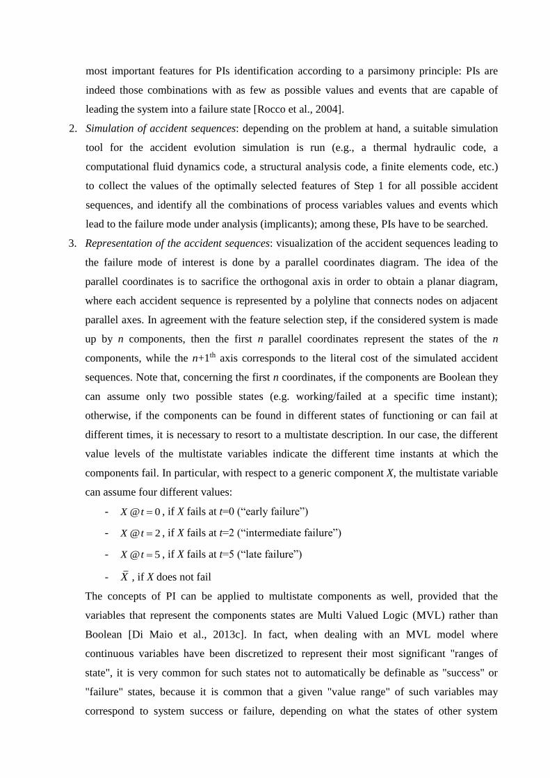
b) PIs selected in a) are removed from the diagram, together with those accident
sequences that are visually verified to be covered by the selected PIs (i.e., implicants
which have the same component states variables defining the removed PI and other
values for the variables whose component state is not defined into the removed PI (or
it is a “do not care” value)). As an example, in Fig. 1 an application of this pruning is
shown for a group of 25 accident sequences, in which the states of components C, D
and E are the same in all the sequences, whereas each sequence has a different
combination of the states of components A and B, which can be in any state. The
sequence with the minimal literal cost is selected as PI and it is shown in continuous
line: it covers all accident sequences where C, D fail at t=0 and E does not fail. The
sequences (Implicants) shown in dashed lines can then be directly removed from the
plot, because they are covered by the solid line PI, independently of the states of A
and B. It is worth noticing that, when the number of accident sequences grows for
very complex systems with a large number of components and states, the method for
retrieving (mining) the PI from the set of implicants is easily applicable because any
implicant sharing the accident sequence characteristics of the identified PI (but with
larger literal cost) will be covered by the identified PI.
c) Step a) and b) must be repeated on the remaining accident sequences until none is
left on the diagram.
At the end, the stored accident sequences are the PIs for the system failure mode under analysis.
Fig. 1. Visualization of the pruning procedure on a parallel coordinates diagram
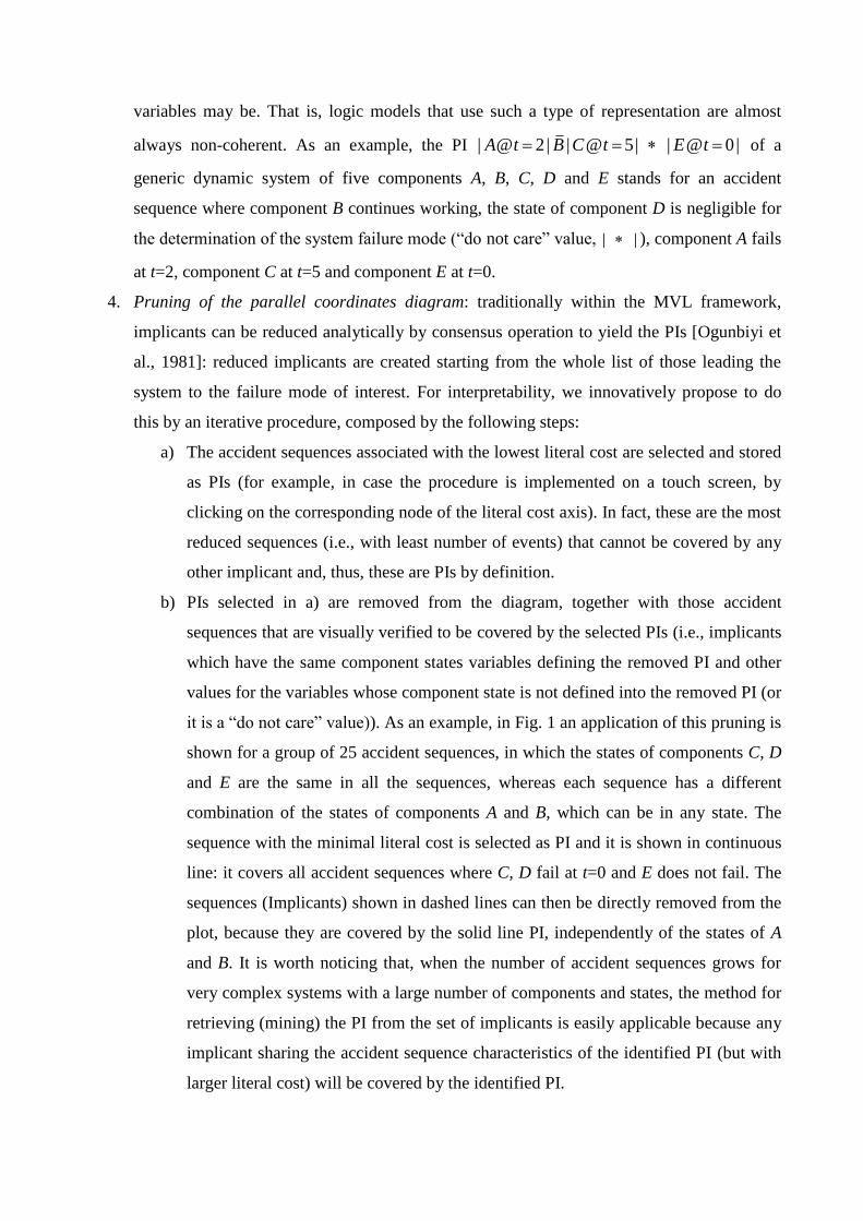
3. ARTIFICIAL CASE STUDY
For illustration of the method proposed, we resort to an artificial case study built by simulating
accident sequences for a system composed by 5 components (coded as A, B, C, D and E) that can
fail at pre-defined discrete times, giving rise to different sequences whose evolutions are
represented by a monitored safety-relevant signal [Di Maio et al., 2013a]. Multiple component
failures can occur during the system life, set to T=7 [h]. Each of the 5 components can fail at t=0,
t=2 and t=5; therefore, the possible component states are: “No failure”, “Failure at t=0”, “Failure at
t=2”, “Failure at t=5”. The equations used to simulate the safety-relevant signal evolution y(t)
during each of the system configurations are shown in Tab. 1. The values of c, d, α1, α2 and α3 are
listed in Tab. 2 and contribute to determining the magnitude of the failure events of the components
A, B, C, D and E.
Failed Component Safety-relevant signal
A 1( ) 2 1
2
ty t erf
B 1( ) 2 1
2
ty t erf
C 2( )
tdy t c c
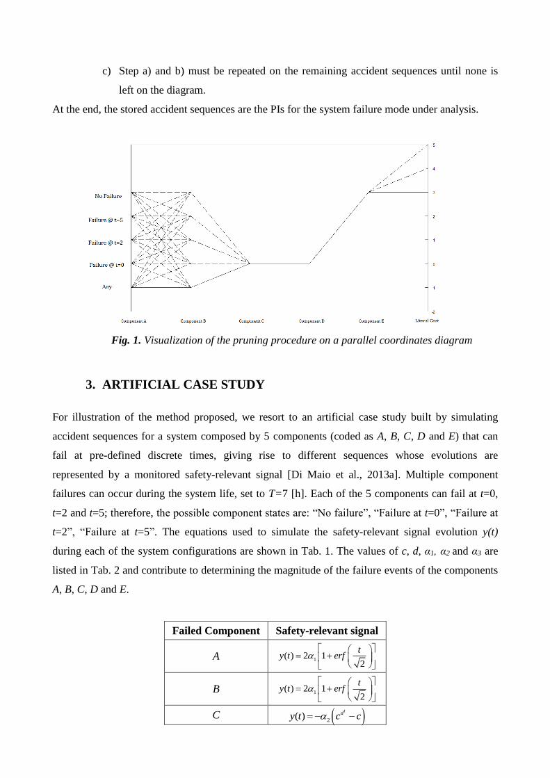
D 2( )
tdy t c c
E 3( )y t t
Tab. 1. Equations used to simulate the safety-relevant signal evolution for each failed component
Parameter Value (in arbitrary units)
1 0.4
2 1.05
3 0.4
c 1.3
d 1.3
Tab. 2. Parameters value
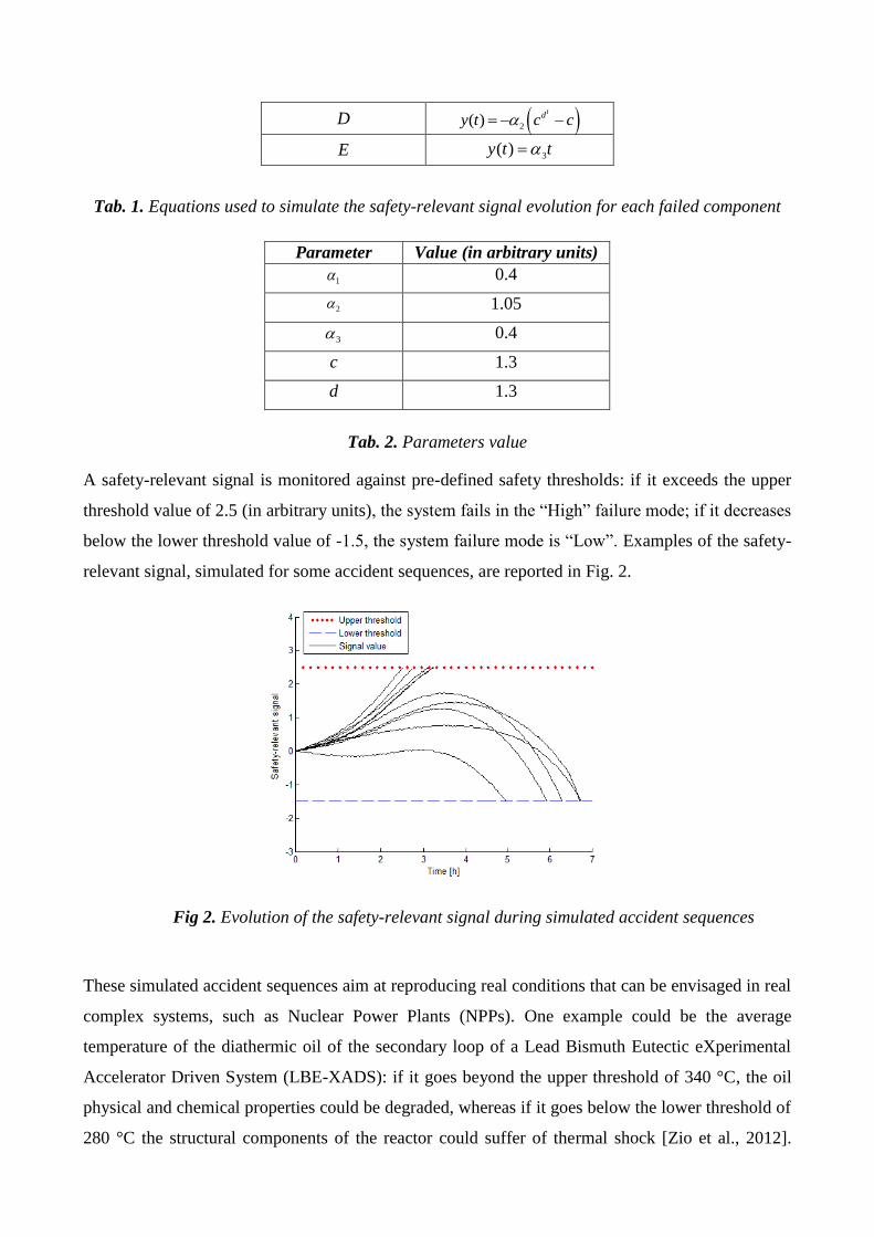
A safety-relevant signal is monitored against pre-defined safety thresholds: if it exceeds the upper
threshold value of 2.5 (in arbitrary units), the system fails in the “High” failure mode; if it decreases
below the lower threshold value of -1.5, the system failure mode is “Low”. Examples of the safety-
relevant signal, simulated for some accident sequences, are reported in Fig. 2.
Fig 2. Evolution of the safety-relevant signal during simulated accident sequences
These simulated accident sequences aim at reproducing real conditions that can be envisaged in real
complex systems, such as Nuclear Power Plants (NPPs). One example could be the average
temperature of the diathermic oil of the secondary loop of a Lead Bismuth Eutectic eXperimental
Accelerator Driven System (LBE-XADS): if it goes beyond the upper threshold of 340 °C, the oil
physical and chemical properties could be degraded, whereas if it goes below the lower threshold of
280 °C the structural components of the reactor could suffer of thermal shock [Zio et al., 2012].
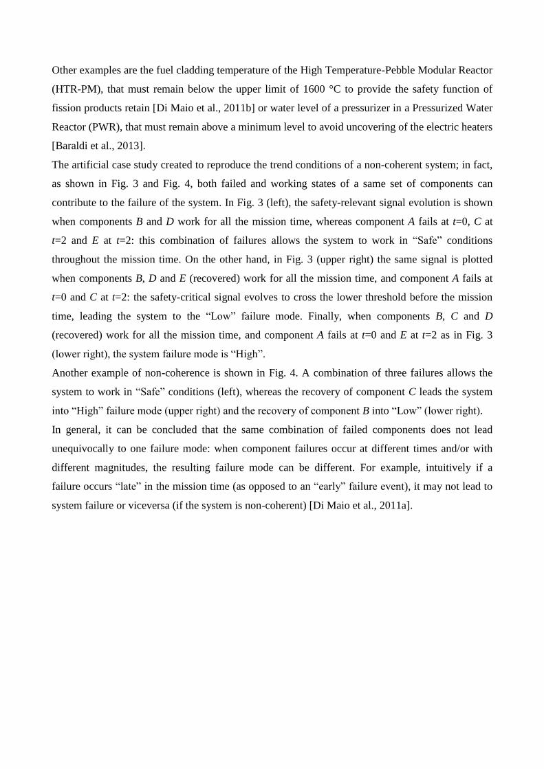
Other examples are the fuel cladding temperature of the High Temperature-Pebble Modular Reactor
(HTR-PM), that must remain below the upper limit of 1600 °C to provide the safety function of
fission products retain [Di Maio et al., 2011b] or water level of a pressurizer in a Pressurized Water
Reactor (PWR), that must remain above a minimum level to avoid uncovering of the electric heaters
[Baraldi et al., 2013].
The artificial case study created to reproduce the trend conditions of a non-coherent system; in fact,
as shown in Fig. 3 and Fig. 4, both failed and working states of a same set of components can
contribute to the failure of the system. In Fig. 3 (left), the safety-relevant signal evolution is shown
when components B and D work for all the mission time, whereas component A fails at t=0, C at
t=2 and E at t=2: this combination of failures allows the system to work in “Safe” conditions
throughout the mission time. On the other hand, in Fig. 3 (upper right) the same signal is plotted
when components B, D and E (recovered) work for all the mission time, and component A fails at
t=0 and C at t=2: the safety-critical signal evolves to cross the lower threshold before the mission
time, leading the system to the “Low” failure mode. Finally, when components B, C and D
(recovered) work for all the mission time, and component A fails at t=0 and E at t=2 as in Fig. 3
(lower right), the system failure mode is “High”.
Another example of non-coherence is shown in Fig. 4. A combination of three failures allows the
system to work in “Safe” conditions (left), whereas the recovery of component C leads the system
into “High” failure mode (upper right) and the recovery of component B into “Low” (lower right).
In general, it can be concluded that the same combination of failed components does not lead
unequivocally to one failure mode: when component failures occur at different times and/or with
different magnitudes, the resulting failure mode can be different. For example, intuitively if a
failure occurs “late” in the mission time (as opposed to an “early” failure event), it may not lead to
system failure or viceversa (if the system is non-coherent) [Di Maio et al., 2011a].

Fig 3. Example of non-coherence
Fig. 4. Example of non-coherence
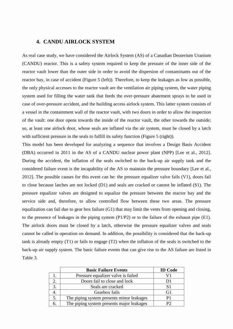
4. CANDU AIRLOCK SYSTEM
As real case study, we have considered the Airlock System (AS) of a Canadian Deuterium Uranium
(CANDU) reactor. This is a safety system required to keep the pressure of the inner side of the
reactor vault lower than the outer side in order to avoid the dispersion of contaminants out of the
reactor bay, in case of accident (Figure 5 (left)). Therefore, to keep the leakages as low as possible,
the only physical accesses to the reactor vault are the ventilation air piping system, the water piping
system used for filling the water tank that feeds the over-pressure abatement sprays to be used in
case of over-pressure accident, and the building access airlock system. This latter system consists of
a vessel in the containment wall of the reactor vault, with two doors in order to allow the inspection
of the vault: one door opens towards the inside of the reactor vault, the other towards the outside;
so, at least one airlock door, whose seals are inflated via the air system, must be closed by a latch
with sufficient pressure in the seals to fulfill its safety function (Figure 5 (right)).
This model has been developed for analyzing a sequence that involves a Design Basis Accident
(DBA) occurred in 2011 in the AS of a CANDU nuclear power plant (NPP) [Lee et al., 2012].
During the accident, the inflation of the seals switched to the back-up air supply tank and the
considered failure event is the incapability of the AS to maintain the pressure boundary [Lee et al.,
2012]. The possible causes for this event can be: the pressure equalizer valve fails (V1), doors fail
to close because latches are not locked (D1) and seals are cracked or cannot be inflated (S1). The
pressure equalizer valves are designed to equalize the pressure between the reactor bay and the
service side and, therefore, to allow controlled flow between these two areas. The pressure
equalization can fail due to gear box failure (G1) that may limit the vents from opening and closing,
to the presence of leakages in the piping system (P1/P2) or to the failure of the exhaust pipe (E1).
The airlock doors must be closed by a latch, otherwise the pressure equalizer valves and seals
cannot be called in operation on demand. In addition, the possibility is considered that the back-up
tank is already empty (T1) or fails to engage (T2) when the inflation of the seals is switched to the
back-up air supply system. The basic failure events that can give rise to the AS failure are listed in
Table 3.
Basic Failure Events ID Code
1. Pressure equalizer valve is failed V1
2. Doors fail to close and lock D1
3. Seals are cracked S1
4. Gearbox fails G1
5. The piping system presents minor leakages P1
6. The piping system presents major leakages P2
7. Exhaust pipe fails open E1
8. Back up tank is empty T1
9. Back up tank fails to engage T2
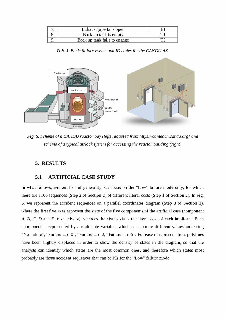
Tab. 3. Basic failure events and ID codes for the CANDU AS.
Fig. 5. Scheme of a CANDU reactor bay (left) [adapted from https://canteach.candu.org] and
scheme of a typical airlock system for accessing the reactor building (right)
5. RESULTS
5.1 ARTIFICIAL CASE STUDY
In what follows, without loss of generality, we focus on the “Low” failure mode only, for which
there are 1166 sequences (Step 2 of Section 2) of different literal costs (Step 1 of Section 2). In Fig.
6, we represent the accident sequences on a parallel coordinates diagram (Step 3 of Section 2),
where the first five axes represent the state of the five components of the artificial case (component
A, B, C, D and E, respectively), whereas the sixth axis is the literal cost of each implicant. Each
component is represented by a multistate variable, which can assume different values indicating
“No failure”, “Failure at t=0”, “Failure at t=2, “Failure at t=5”. For ease of representation, polylines
have been slightly displaced in order to show the density of states in the diagram, so that the
analysts can identify which states are the most common ones, and therefore which states most
probably are those accident sequences that can be PIs for the “Low” failure mode.
Ventilation air
Building
access airlock
Reactor
Dousing sprays
Dousing tank
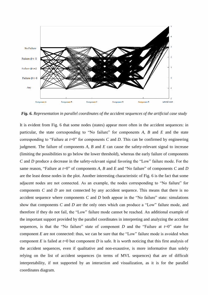
Fig. 6. Representation in parallel coordinates of the accident sequences of the artificial case study
It is evident from Fig. 6 that some nodes (states) appear more often in the accident sequences: in
particular, the state corresponding to “No failure” for components A, B and E and the state
corresponding to “Failure at t=0” for components C and D. This can be confirmed by engineering
judgment. The failure of components A, B and E can cause the safety-relevant signal to increase
(limiting the possibilities to go below the lower threshold), whereas the early failure of components
C and D produce a decrease in the safety-relevant signal favoring the “Low” failure mode. For the
same reason, “Failure at t=0” of components A, B and E and “No failure” of components C and D
are the least dense nodes in the plot. Another interesting characteristic of Fig. 6 is the fact that some
adjacent nodes are not connected. As an example, the nodes corresponding to “No failure” for
components C and D are not connected by any accident sequence. This means that there is no
accident sequence where components C and D both appear in the “No failure” state: simulations
show that components C and D are the only ones which can produce a “Low” failure mode, and
therefore if they do not fail, the “Low” failure mode cannot be reached. An additional example of
the important support provided by the parallel coordinates in interpreting and analyzing the accident
sequences, is that the “No failure” state of component D and the “Failure at t=0” state for
component E are not connected: thus, we can be sure that the “Low” failure mode is avoided when
component E is failed at t=0 but component D is safe. It is worth noticing that this first analysis of
the accident sequences, even if qualitative and non-exaustive, is more informative than solely
relying on the list of accident sequences (in terms of MVL sequences) that are of difficult
interpretability, if not supported by an interaction and visualization, as it is for the parallel
coordinates diagram.

After the qualitative analysis of the accident sequences, we can move to Step 4 of Section 2. If we
select from Fig. 6 the accident sequences with the minimal literal cost (equal to 3), we identify 69
PIs, (reported in Appendix A in rows from 1 to 69). Then, we can delete the 69 PIs from Fig. 6,
together with the sequences that they cover. The remaining sequences are showed in Fig. 7.
Fig. 7. Visualization of the results of the first iteration of the pruning step on the accident sequences
of the artificial case study
In the second iteration, the 101 implicants with the second lowest literal cost (equal to 4) are
selected from Fig. 7 as PIs (Appendix A, rows from 70 to 170). Then, we can delete the 101 PIs
from Fig. 6, together with the sequences that they cover. The remaining sequences are showed in
Fig. 8.

Fig. 8. Visualization of the results of the second iteration of the pruning step on the accident
sequences of the artificial case study
It is evident from Fig. 8 that all 10 sequences that are left on the plot have the same minimal literal
cost, and they are all stored as PIs (Appendix A, rows from 171 to 180). Then, pruning is terminated
and 180 PIs of the “Low” failure mode of the system have been found (Appendix A).
In order to validate the results obtained by the visual interactive method, we resort to an analytical
technique, the consensus method for identifying PIs [Ogunbiyi et al., 1981]. With this algorithm, we
can identify the PIs from all the accident sequences by consensus operation: reduced implicants are
created starting from the whole list of those leading the system to the failure mode of interest. The
basic simplifying operation, called merging rule, is: if s implicants are the same except for exactly
one s-th event entry (where s is the number of states that the variables that represent each
component can assume, equal to 4 in this case), and all the s possible states of the input variable
exist in these implicants, then the s implicants can be merged and form a more reduced implicant
[Ogunbiyi et al., 1981]. In Tab. 4 an example of the merging rule is shown: 4 implicants are listed
where components B, C, D and E appear in the same state (B failed at t=5, C failed at t=0, D failed
at t=0 and E working), while component A appears with a different state in each implicant. By
application of the merging rule, a reduced implicant is obtained, as reported in the last row of Tab.
3.
A @ 5B t @ 0C t @ 0D t E
@ 0A t @ 5B t @ 0C t @ 0D t E
@ 2A t @ 5B t @ 0C t @ 0D t E
@ 5A t @ 5B t @ 0C t @ 0D t E
- @ 5B t @ 0C t @ 0D t E
Tab. 4. Example of application of the merging rule
The PIs identification by consensus operation proceeds iteratively to the reduction of the list of
implicants until all PIs are found (in ~2 seconds on an Intel Core2Duo P7550). In the artificial case
study considered, the consensus method finds the same PIs for the “Low” failure mode as obtained
by the proposed visual interactive method, but, in addition to the former one, the latter offers greatly
improved interpretability of the results and insightful information for qualitative analysis of the
accident sequences (as previously discussed), thanks to the proper selection of the features
characterizing the accident sequences and the straightforward algorithm for pruning the parallel
coordinates diagram based on the information of the literal cost of the accident sequences (whose
results are obtained in in ~1.5 seconds on an Intel Core2Duo P7550, that is i) comparable to other
PI identification methods, and ii) accounts for the 25% savings of computational time when applied
on a problem of up-scaled complexity with respect to the consensus method).
5.2 CANDU AIRLOCK SYSTEM
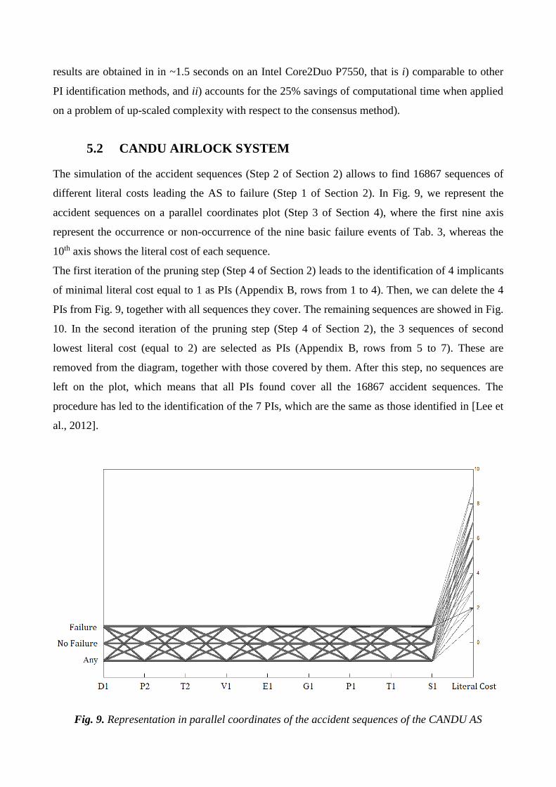
The simulation of the accident sequences (Step 2 of Section 2) allows to find 16867 sequences of
different literal costs leading the AS to failure (Step 1 of Section 2). In Fig. 9, we represent the
accident sequences on a parallel coordinates plot (Step 3 of Section 4), where the first nine axis
represent the occurrence or non-occurrence of the nine basic failure events of Tab. 3, whereas the
10th axis shows the literal cost of each sequence.
The first iteration of the pruning step (Step 4 of Section 2) leads to the identification of 4 implicants
of minimal literal cost equal to 1 as PIs (Appendix B, rows from 1 to 4). Then, we can delete the 4
PIs from Fig. 9, together with all sequences they cover. The remaining sequences are showed in Fig.
10. In the second iteration of the pruning step (Step 4 of Section 2), the 3 sequences of second
lowest literal cost (equal to 2) are selected as PIs (Appendix B, rows from 5 to 7). These are
removed from the diagram, together with those covered by them. After this step, no sequences are
left on the plot, which means that all PIs found cover all the 16867 accident sequences. The
procedure has led to the identification of the 7 PIs, which are the same as those identified in [Lee et
al., 2012].
Fig. 9. Representation in parallel coordinates of the accident sequences of the CANDU AS
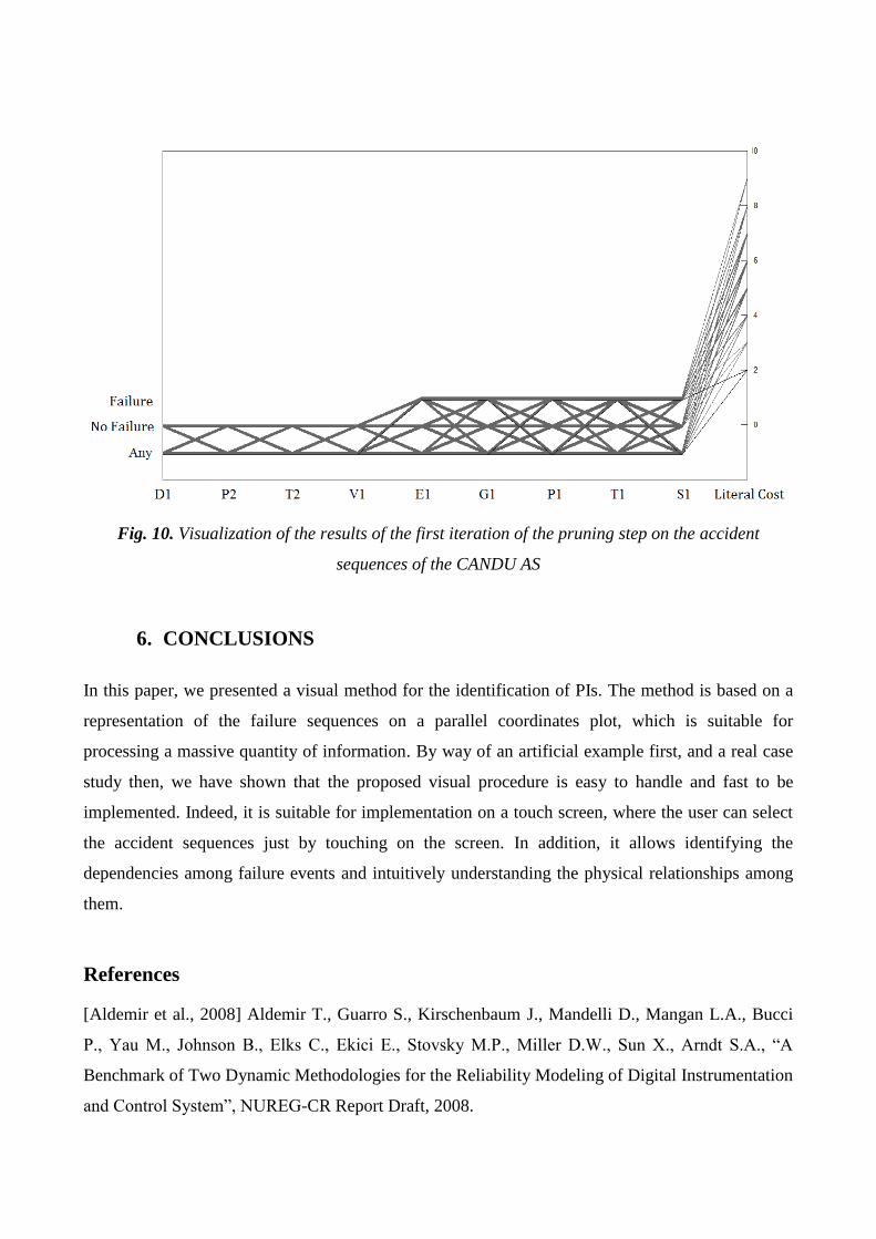
Fig. 10. Visualization of the results of the first iteration of the pruning step on the accident
sequences of the CANDU AS
6. CONCLUSIONS
In this paper, we presented a visual method for the identification of PIs. The method is based on a
representation of the failure sequences on a parallel coordinates plot, which is suitable for
processing a massive quantity of information. By way of an artificial example first, and a real case
study then, we have shown that the proposed visual procedure is easy to handle and fast to be
implemented. Indeed, it is suitable for implementation on a touch screen, where the user can select
the accident sequences just by touching on the screen. In addition, it allows identifying the
dependencies among failure events and intuitively understanding the physical relationships among
them.
References
[Aldemir et al., 2008] Aldemir T., Guarro S., Kirschenbaum J., Mandelli D., Mangan L.A., Bucci
P., Yau M., Johnson B., Elks C., Ekici E., Stovsky M.P., Miller D.W., Sun X., Arndt S.A., “A
Benchmark of Two Dynamic Methodologies for the Reliability Modeling of Digital Instrumentation
and Control System”, NUREG-CR Report Draft, 2008.
[Aldemir, 2013] Aldemir T., “A survey of dynamic methodologies for probabilistic safety
assessment of nuclear power plant”, Annals of Nuclear Energy, Volume 52, pp.113-124, 2013.
[Baraldi et al., 2013] Baraldi P., Di Maio F., Zio E., “Unsupervised Clustering for Fault Diagnosis
in Nuclear Power Plant Components”, International Journal of Computational Intelligence Systems,
Vol. 6, No. 4, July 2013, pp. 764-777..
[Beeson, 2002] Beeson S.C., “Non-coherent fault tree analysis”, Loughborough University UK.
[Bell et al., 1986] Bell P.C., O’Keefe R.M, “Visual Interactive Simulation – History, Recent
Develpments, and Major Issues”, SIMULATION, N0. 49, pp.109-116, 1987.
[Buja et al., 1985] Buja A., Asimov D., “Grand tour methods: an outline”, Computer Science and
Statistics: Proceedings of the Seventeenth Symposium on the Interface, D. Allen, ed., North
Holland, Amsterdam, pp.63-67, 1985.
[Coudert et al., 1992] Coudert, O., Madre, J.C., “Implicit and incremental computation of primes
and essential primes of Boolean functions”, Proceedings of the 29th ACM/IEEE Design
Automation Conference, Anaheim, CA, USA, 8-12 June, 1992, Pages 36-39.
[Devooght et al., 1992] Devooght D., Smidts C., “Probabilistic reactor dynamics I: the theory of
continuous event trees”, Nuclear Science and Engineering, Volume 111, pp.229-240, 1992.
[Di Maio et al., 2011a] Di Maio F., Secchi P., Vantini S., Zio E., “Fuzzy C-Means Clustering of
Signal Functional Principal Components for Post-Processing Dynamic Sequences of a Nuclear
Power Plant Digital Instrumentation and Control System”, IEEE Transactions on Reliability,
pp.415-425, 2011.
[Di Maio et al., 2011b] Di Maio F., Zio E., Jiejuan Tong T.L., “Passive system accident sequence
analysis by simulation”, ANS PSA 2011 International Topical Meeting on Probabilistic Safety
Assessment and Analysis, Wilmington, NC, March 13-17, 2011.
[Di Maio et al., 2013a] Di Maio F., Baronchelli S., Zio E., “Prime Implicants Determination by
Differential Evolution for Dynamic Reliability Analysis of Non-Coherent Systems”, under review,
Reliability Engineering and System Safety.
[Di Maio et al., 2013b] F. Di Maio, S. Baronchelli, E. Zio, “Minimal Cut Sets Identification by
Hierarchical Differential Evolution”, PSA 2013, the International Topical Meeting on Probabilistic
Safety Assessment and Analysis, 22-27 September 2013, Columbia, South Carolina, USA.
[Di Maio et al., 2013c] F. Di Maio, S. Baronchelli, E. Zio, “Hierarchical Differential Evolution for
Minimal Cut Sets Identification: Application to Nuclear Safety Systems”, accepted, European
Journal of Operational Research.
[Guarro et al., 2012] S. Guarro, M. Yau and S. Dixon, “Applications of the Dynamic Flowgraph
Methodology to Dynamic Modeling and Analysis” Proceedings of the 11th International

Conference on Probabilistic Safety Assessment and Management (PSAM 11), Helsinki, Finland,
June 25-29, 2012.
[Hurrion, 1980] Hurrion R.D., “An interactive visual simulation System for Industrial
Management”, European Journal of Operational Research, Volume 5, pp.86-93, 1980.
[Karnaugh, 1953] Karnaugh M., "The Map Method for Synthesis of Combinational Logic
Circuits", Transactions of the American Institute for Electrical Engineers part I 72 (9): 593–599,
1953.
[Inselberg, 1985] Inselberg A., “The plane with parallel coordinates”, The Visual Computer,
Volume 1, pp.69-91, 1985.
[Lee et al., 2012] Lee A., Lu L., “Petri Net Modeling for Probabilistic Safety Assessment and its
Application in the Air Lock System of a CANDU Nuclear Power Plant”, Procedia Engineering,
2012 International Symposium on Safey Science and Technology, Volume 25, pp.11-20, 2012.
[Marshall et al., 1990] Marshall R., Kempf J., Dyer S., Yan C., “Visualization Methods and
Simulation Steering for a 3D Turbulence Model of the Lake Erie”, Computer Graphics, Volume 24
(2), pp.89-97, 1990.
[McCluskey, 1956] McCluskey E.J.Jr. , “Minimization of Boolean functions”, Bell Sys. Tech. J.,
Volume 35, 1417-1444, 1956.
[Ogunbiyi et al., 1981] Ogunbiyi E.I., Henley E.J., “Irredundant Forms and Prime Implicants of a
Function with Multistate Variables”, IEEE Transactions on Reliability, Volume R-30, No. 1, pp.39-
42, 1981.
[Quine, 1952] Quine W.V., “The problem of simplifying truth functions”, Am. Math. Monthly,
Volume 59, 521-531, 1952.
[Rauzy et al, 1997] Rauzy, A., Dutuit, Y., “Exact and truncated computations of prime Implicants
of coherent and non-coherent fault tree”, Reliability Engineering and System Safety, 58, 127-144.
[Rocco et al., 2004] Rocco C.M., Muselli M., “A Machine Learning Algorithm to Estimate Minimal
Cut and Path Sets from a Monte Carlo Simulation”, Proceedings Probabilistic Safety Assessment
and Management PSAM7/ESREL’04, 2008.
[Schramm et al., 2007] Schramm F.K., Formoso C.T., “Using Visual Interactive Simulation to
improve decision-making in production”, Proceedings IGLC-15, July 2007, Michigan, USA,
pp.357-366, 2007.
[Sen, 1993] Sen S., “Minimal cost set covering using probabilistic methods”, Proceedings of the
1993 ACM/SIGAPP symposium on Applied computing: states of the art and practice, 157-164,
1993.
[Sharvia et al., 2008] Sharvia S., Papadopoulos, “Non-coherent Modelling in Compositional Fault
Tree Analysis”, Proceedings of the 17th World Congress, The International Federation of
Automatic Control, Seoul, Korea, July 6-11, 2008.
[Wagner et al., 1996] Wagner P.R., Dal Sasso C.M., Wagner F., “A new paradigm for Visual
Interactive Modeling and Simulation”, European Simulation Symposium, 1996.
[Wegman et al., 1997] Wegman E., Luo Q., “High dimensional clustering using parallel coordinates
and the grand tour”, Computing Science and Statistics, Volume 28, pp.352-360, 1997.
[Wegman, 2003] Wegman E.J., “Visual Data Mining”, Statistics in Medicine, Volume 22, No. 9,
pp.1383-1397, 2003.
[Worrell et al., 1981] Worrell R.B., Stack D.W., Hulme B.L., “Prime implicant of non-coherent
fault trees”, IEEE Transactions on Reliability R-30/2, 98-100, 1981.
[Yau et al., 1998] M. Yau, G. Apostolakis and S. Guarro, “The Use of Prime Implicants in
Dependability Analysis of Software Controlled Systems”, Reliability Engineering and System
Safety, 62, pp. 11-32, 1998.
[Zio et al., 2009] Zio E., Di Maio F., “Processing Dynamic Sequences from a Reliability Analysis
of a Nuclear Power Plant Digital Instrumentation and Control System”, Annals of Nuclear Energy
36, 1386-1399, 2009.
[Zio et al., 2012] Zio E., Di Maio F., “Fault Diagnosis and Failure Mode Estimation Data-Driven
Fuzzy Similarity Approach”, International Journal of Performability Engineering, Volume 8, No. 1,
pp.49-65, 2012.
[Zhou et al., 2008] Zhou H., Yuan X., Qu H., Chen B., “Visual Clustering in Parallel Coordinates”,
IEEE-VGTC Symposium on Visualization 2008, Volume 27, No. 3, 2008.
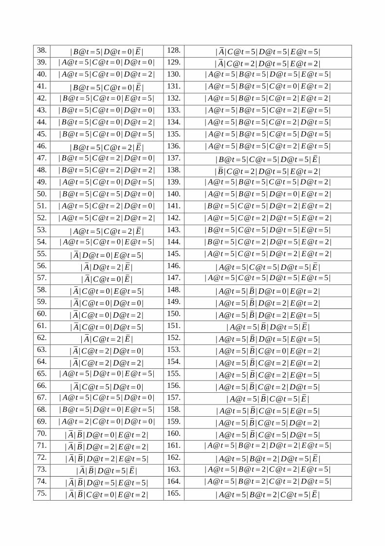
APPENDIX A
For the artificial case study, the list of PIs for the “Low” failure mode, identified through the visual
interactive method is reported below. The state of component X (where X stands for the component
code) can assume four different values:
- @ 0X t , if X fails at t=0
- @ 2X t , if X fails at t=2
- @ 5X t , if X fails at t=5
- X , if X does not fail.
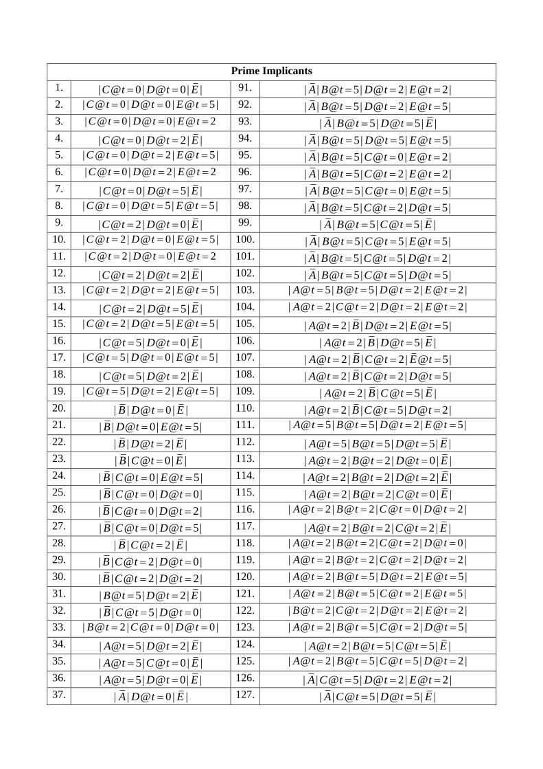
Prime Implicants
1. | @ 0| @ 0| |C t D t E 91. | | @ 5| @ 2| @ 2|A B t D t E t
2. | @ 0 | @ 0 | @ 5|C t D t E t 92. | | @ 5| @ 2| @ 5|A B t D t E t
3. | @ 0 | @ 0 | @ 2C t D t E t 93. | | @ 5| @ 5| |A B t D t E
4. | @ 0| @ 2| |C t D t E 94. | | @ 5| @ 5| @ 5|A B t D t E t
5. | @ 0 | @ 2 | @ 5|C t D t E t 95. | | @ 5| @ 0| @ 2|A B t C t E t
6. | @ 0 | @ 2 | @ 2C t D t E t 96. | | @ 5| @ 2| @ 2|A B t C t E t
7. | @ 0| @ 5| |C t D t E 97. | | @ 5| @ 0| @ 5|A B t C t E t
8. | @ 0 | @ 5| @ 5|C t D t E t 98. | | @ 5| @ 2| @ 5|A B t C t D t
9. | @ 2| @ 0| |C t D t E 99. | | @ 5| @ 5| |A B t C t E
10. | @ 2 | @ 0 | @ 5|C t D t E t 100. | | @ 5| @ 5| @ 5|A B t C t E t
11. | @ 2 | @ 0 | @ 2C t D t E t 101. | | @ 5| @ 5| @ 2|A B t C t D t
12. | @ 2| @ 2| |C t D t E 102. | | @ 5| @ 5| @ 5|A B t C t D t
13. | @ 2 | @ 2 | @ 5|C t D t E t 103. | @ 5| @ 5| @ 2 | @ 2 |A t B t D t E t
14. | @ 2| @ 5| |C t D t E 104. | @ 2 | @ 2 | @ 2 | @ 2 |A t C t D t E t
15. | @ 2 | @ 5| @ 5|C t D t E t 105. | @ 2| | @ 2| @ 5|A t B D t E t
16. | @ 5| @ 0| |C t D t E 106. | @ 2| | @ 5| |A t B D t E
17. | @ 5| @ 0 | @ 5|C t D t E t 107. | @ 2| | @ 2| @ 5|A t B C t E t
18. | @ 5| @ 2| |C t D t E 108. | @ 2| | @ 2| @ 5|A t B C t D t
19. | @ 5| @ 2 | @ 5|C t D t E t 109. | @ 2| | @ 5| |A t B C t E
20. | | @ 0| |B D t E 110. | @ 2| | @ 5| @ 2|A t B C t D t
21. | | @ 0| @ 5|B D t E t 111. | @ 5| @ 5| @ 2 | @ 5|A t B t D t E t
22. | | @ 2| |B D t E 112. | @ 5| @ 5| @ 5| |A t B t D t E
23. | | @ 0| |B C t E 113. | @ 2| @ 2| @ 0| |A t B t D t E
24. | | @ 0| @ 5|B C t E t 114. | @ 2| @ 2| @ 2| |A t B t D t E
25. | | @ 0| @ 0|B C t D t 115. | @ 2| @ 2| @ 0| |A t B t C t E
26. | | @ 0| @ 2|B C t D t 116. | @ 2 | @ 2 | @ 0 | @ 2 |A t B t C t D t
27. | | @ 0| @ 5|B C t D t 117. | @ 2| @ 2| @ 2| |A t B t C t E
28. | | @ 2| |B C t E 118. | @ 2 | @ 2 | @ 2 | @ 0 |A t B t C t D t
29. | | @ 2| @ 0|B C t D t 119. | @ 2 | @ 2 | @ 2 | @ 2 |A t B t C t D t
30. | | @ 2| @ 2|B C t D t 120. | @ 2 | @ 5| @ 2 | @ 5|A t B t D t E t
31. | @ 5| @ 2| |B t D t E 121. | @ 2 | @ 5| @ 2 | @ 5|A t B t C t E t
32. | | @ 5| @ 0|B C t D t 122. | @ 2 | @ 2 | @ 2 | @ 2 |B t C t D t E t
33. | @ 2 | @ 0 | @ 0 |B t C t D t 123. | @ 2 | @ 5| @ 2 | @ 5|A t B t C t D t
34. | @ 5| @ 2| |A t D t E 124. | @ 2| @ 5| @ 5| |A t B t C t E
35. | @ 5| @ 0| |A t C t E 125. | @ 2 | @ 5| @ 5| @ 2 |A t B t C t D t
36. | @ 5| @ 0| |A t D t E 126. | | @ 5| @ 2| @ 2|A C t D t E t
37. | | @ 0| |A D t E 127. | | @ 5| @ 5| |A C t D t E
38. | @ 5| @ 0| |B t D t E 128. | | @ 5| @ 5| @ 5|A C t D t E t
39. | @ 5| @ 0 | @ 0 |A t C t D t 129. | | @ 2| @ 5| @ 2|A C t D t E t
40. | @ 5| @ 0 | @ 2 |A t C t D t 130. | @ 5| @ 5| @ 5| @ 5|A t B t D t E t
41. | @ 5| @ 0| |B t C t E 131. | @ 5| @ 5| @ 0 | @ 2 |A t B t C t E t
42. | @ 5| @ 0 | @ 5|B t C t E t 132. | @ 5| @ 5| @ 2 | @ 2 |A t B t C t E t
43. | @ 5| @ 0 | @ 0 |B t C t D t 133. | @ 5| @ 5| @ 2 | @ 5|A t B t C t E t
44. | @ 5| @ 0 | @ 2 |B t C t D t 134. | @ 5| @ 5| @ 2 | @ 5|A t B t C t D t
45. | @ 5| @ 0 | @ 5|B t C t D t 135. | @ 5| @ 5| @ 5| @ 5|A t B t C t D t
46. | @ 5| @ 2| |B t C t E 136. | @ 5| @ 5| @ 2 | @ 5|A t B t C t E t
47. | @ 5| @ 2 | @ 0 |B t C t D t 137. | @ 5| @ 5| @ 5| |B t C t D t E
48. | @ 5| @ 2 | @ 2 |B t C t D t 138. | | @ 2| @ 5| @ 2|B C t D t E t
49. | @ 5| @ 0 | @ 5|A t C t D t 139. | @ 5| @ 5| @ 5| @ 2 |A t B t C t D t
50. | @ 5| @ 5| @ 0 |B t C t D t 140. | @ 5| @ 5| @ 0 | @ 2 |A t B t D t E t
51.
| @ 5| @ 2 | @ 0 |A t C t D t 141. | @ 5| @ 5| @ 2 | @ 2 |B t C t D t E t
52. | @ 5| @ 2 | @ 2 |A t C t D t 142. | @ 5| @ 2 | @ 5| @ 2 |A t C t D t E t
53. | @ 5| @ 2| |A t C t E 143. | @ 5| @ 5| @ 5| @ 5|B t C t D t E t
54. | @ 5| @ 0 | @ 5|A t C t E t 144. | @ 5| @ 2 | @ 5| @ 2 |B t C t D t E t
55. | | @ 0| @ 5|A D t E t 145. | @ 5| @ 5| @ 2 | @ 2 |A t C t D t E t
56. | | @ 2| |A D t E 146. | @ 5| @ 5| @ 5| |A t C t D t E
57. | | @ 0| |A C t E 147. | @ 5| @ 5| @ 5| @ 5|A t C t D t E t
58. | | @ 0| @ 5|A C t E t 148. | @ 5| | @ 0| @ 2|A t B D t E t
59. | | @ 0| @ 0|A C t D t 149. | @ 5| | @ 2| @ 2|A t B D t E t
60. | | @ 0| @ 2|A C t D t 150. | @ 5| | @ 2| @ 5|A t B D t E t
61. | | @ 0| @ 5|A C t D t 151. | @ 5| | @ 5| |A t B D t E
62. | | @ 2| |A C t E 152. | @ 5| | @ 5| @ 5|A t B D t E t
63. | | @ 2| @ 0|A C t D t 153. | @ 5| | @ 0| @ 2|A t B C t E t
64. | | @ 2| @ 2|A C t D t 154. | @ 5| | @ 2| @ 2|A t B C t E t
65. | @ 5| @ 0 | @ 5|A t D t E t 155. | @ 5| | @ 2| @ 5|A t B C t E t
66. | | @ 5| @ 0|A C t D t 156. | @ 5| | @ 2| @ 5|A t B C t D t
67. | @ 5| @ 5| @ 0 |A t C t D t 157. | @ 5| | @ 5| |A t B C t E
68. | @ 5| @ 0 | @ 5|B t D t E t 158. | @ 5| | @ 5| @ 5|A t B C t E t
69. | @ 2 | @ 0 | @ 0 |A t C t D t 159. | @ 5| | @ 5| @ 2|A t B C t D t
70. | | | @ 0| @ 2|A B D t E t 160. | @ 5| | @ 5| @ 5|A t B C t D t
71. | | | @ 2| @ 2|A B D t E t 161. | @ 5| @ 2 | @ 2 | @ 5|A t B t D t E t
72. | | | @ 2| @ 5|A B D t E t 162. | @ 5| @ 2| @ 5| |A t B t D t E
73. | | | @ 5| |A B D t E 163. | @ 5| @ 2 | @ 2 | @ 5|A t B t C t E t
74. | | | @ 5| @ 5|A B D t E t 164. | @ 5| @ 2 | @ 2 | @ 5|A t B t C t D t
75. | | | @ 0| @ 2|A B C t E t 165. | @ 5| @ 2| @ 5| |A t B t C t E
76. | | | @ 2| @ 2|A B C t E t 166. | @ 5| @ 2 | @ 5| @ 2 |A t B t C t D t
77. | | | @ 2| @ 5|A B C t E t 167. | | @ 5| @ 2| @ 2|B C t D t E t
78. | | | @ 2| @ 5|A B C t D t 168. | | @ 5| @ 5| |B C t D t E
79. | | | @ 5| |A B C t E 169. | | @ 5| @ 5| @ 5|B C t D t E t
80. | | | @ 5| @ 5|A B C t E t 170. | @ 2| @ 5| @ 5| |A t B t D t E
81. | | | @ 5| @ 2|A B C t D t 171. | @ 2| @ 2| @ 5| @ 5| |A t B t C t D t E
82. | | | @ 5| @ 5|A B C t D t 172. | | @ 2| @ 5| @ 5| @ 2|A B t C t D t E t
83. | | @ 2| @ 2| @ 5|A B t D t E t 173. | @ 2| | @ 5| @ 5| @ 2|A t B C t D t E t
84. | | @ 2| @ 5| |A B t D t E 174. | @ 2 | @ 2 | @ 2 | @ 5| @ 2 |A t B t C t D t E t
85. | | @ 2| @ 2| @ 5|A B t C t E t 175. | @ 2 | @ 2 | @ 5| @ 0 | @ 2 |A t B t C t D t E t
86. | | @ 2| @ 2| @ 5|A B t C t D t 176. | @ 2 | @ 2 | @ 0 | @ 5| @ 2 |A t B t C t D t E t
87. | | @ 2| @ 5| |A B t C t E 177. | @ 2 | @ 2 | @ 5| @ 2 | @ 2 |A t B t C t D t E t
88. | | @ 2| @ 5| @ 2|A B t C t D t 178. | @ 2 | @ 2 | @ 5| @ 5| @ 5|A t B t C t D t E t
89. | @ 5| @ 5| @ 5| |A t B t C t E 179. | @ 2 | @ 5| @ 5| @ 5| @ 2 |A t B t C t D t E t
90. | | @ 5| @ 0| @ 2|A B t D t E t 180. | @ 5| @ 2 | @ 5| @ 5| @ 2 |A t B t C t D t E t
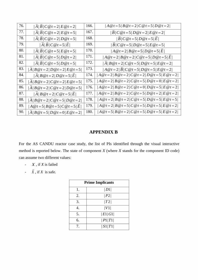
APPENDIX B
For the AS CANDU reactor case study, the list of PIs identified through the visual interactive
method is reported below. The state of component X (where X stands for the component ID code)
can assume two different values:
- X , if X is failed
- X , if X is safe.
Prime Implicants
1. | 1|D
2. | 2 |P
3. | 2 |T
4. | 1|V
5. | 1| 1|E G
6. | 1| 1|P T
7. | 1| 1|S T