a voxel-based approach to the real-time simulation of
TRANSCRIPT

A VOXEL-BASED APPROACH TO THE REAL-TIME SIMULATION
OF SANDS AND SOILS
A Thesis
Submitted to the Faculty of Graduate Studies and Research
In Partial Fulfillment of the Requirements
For the Degree of
Master of Science
in
Computer Science
University of Regina
By
Andrew David Geiger
Regina, Saskatchewan
July, 2015
Copyright 2015: A.D. Geiger

UNIVERSITY OF REGINA
FACULTY OF GRADUATE STUDIES AND RESEARCH
SUPERVISORY AND EXAMINING COMMITTEE
Andrew David Geiger, candidate for the degree of Master of Science in Computer Science, has presented a thesis titled, A Voxel-Based Approach to the Real-Time Simulation of Sands and Soils, in an oral examination held on May 25, 2015. The following committee members have found the thesis acceptable in form and content, and that the candidate demonstrated satisfactory knowledge of the subject material. External Examiner: Dr. Eric Neufeld, University of Saskatchewan
Supervisor: Dr. Howard J. Hamilton, Department of Computer Science
Committee Member: Dr. Robert J. Hilderman, Department of Computer Science
Committee Member: Dr. Xue-Dong Yang, Department of Computer Science
Chair of Defense: Dr. Allen Herman, Department of Mathematics & Statistics

Abstract
Natural terrains composed of sands, soils, and other types of granular materials are
subject to deformation and alteration when influenced by interactions with humans
and machines. These interactions include excavation and earthmoving activities such
as digging, pushing, lifting, dumping, and piling. Simulating the deformation of sand
and soil-filled terrains in interactive computer graphics applications is challenging
due to the fine-grained and highly dynamic nature of these materials. In this thesis,
we present the theoretical background, algorithms, and implementation details for a
voxel-based terrain rendering system that simulates large, dynamic bodies of sands
and soils in real-time 3D graphics applications. We describe a technique for repre-
senting soil in a 3D voxel grid, and we introduce a set of GPU-based algorithms that
simulate the physical behaviors of soils in this representation. A multi-level height-
field is used to track the slopes of the soil-covered surfaces for slope stability analysis
and soil slippage computations. The surfaces of the simulated soils are visualized
each frame by extracting a polygonal mesh from the voxel grid with the Marching
Cubes and Transvoxel algorithms. We show that our proposed algorithm is capable
of producing realistic, high-quality simulations of soils with 3D effects that are not
possible in previous approaches. We also show that our proposed system is capable
of operating in real-time on consumer level GPUs with over 60 frames rendered per
second.
i

Acknowledgements
I would like to thank Dr. Howard Hamilton for his support and guidance through-
out my years as a student, and for offering invaluable insights and advice during my
thesis research. I would also like to thank Jason Selzer and the rest of the team at
Serious Labs for collaborating with us on this project, Stamatis Katsaganis for his
assistance during the development of the ideas and software for this research, and
Drs. Robert Hilderman and Xue Dong Yang for their participation in my supervisory
committee.
ii

Post Defense Acknowledgements
I would like to thank my external examiner, Dr. Eric Neufeld, and the chair of my
defense, Dr. Allen Herman, for their involvement in my thesis defense.
iii

Dedication
I would like to dedicate this work to my parents, Arden and Garth Geiger. With-
out your support, none of this would have been possible. I would also like to thank
my two brothers, Adam and Matt Geiger, for always being there, my friends for
being the best friends anyone could ask for, and Nicole Hagen for her support and
encouragement.
iv

Contents
1 Introduction 1
1.1 Research Goal . . . . . . . . . . . . . . . . . . . . . . . . . . . . . . . 2
1.2 Motivation . . . . . . . . . . . . . . . . . . . . . . . . . . . . . . . . . 5
1.3 Outline . . . . . . . . . . . . . . . . . . . . . . . . . . . . . . . . . . . 7
2 Background 8
2.1 Virtual Soil . . . . . . . . . . . . . . . . . . . . . . . . . . . . . . . . 8
2.1.1 Modeling Soil . . . . . . . . . . . . . . . . . . . . . . . . . . . 8
2.1.2 Soil Slippage . . . . . . . . . . . . . . . . . . . . . . . . . . . . 15
2.2 Voxel-Based Terrain Rendering . . . . . . . . . . . . . . . . . . . . . 22
2.2.1 Terrain Representation . . . . . . . . . . . . . . . . . . . . . . 22
2.2.2 Terrain Generation . . . . . . . . . . . . . . . . . . . . . . . . 24
2.2.3 Terrain Visualization . . . . . . . . . . . . . . . . . . . . . . . 25
2.2.4 Terrain Level of Detail . . . . . . . . . . . . . . . . . . . . . . 29
2.3 Voxel-Based Fluid Simulation . . . . . . . . . . . . . . . . . . . . . . 35
3 Voxel Soil 39
3.1 Representation . . . . . . . . . . . . . . . . . . . . . . . . . . . . . . 39
3.2 Simulation . . . . . . . . . . . . . . . . . . . . . . . . . . . . . . . . . 42
3.2.1 Soil Advection . . . . . . . . . . . . . . . . . . . . . . . . . . . 44
3.2.2 Body Forces . . . . . . . . . . . . . . . . . . . . . . . . . . . . 53
3.2.3 Soil Slippage . . . . . . . . . . . . . . . . . . . . . . . . . . . . 53
3.2.4 Soil Deformation . . . . . . . . . . . . . . . . . . . . . . . . . 62
3.3 Visualization . . . . . . . . . . . . . . . . . . . . . . . . . . . . . . . 70
3.4 Implementation . . . . . . . . . . . . . . . . . . . . . . . . . . . . . . 73
v

3.4.1 Development Environment . . . . . . . . . . . . . . . . . . . . 73
3.4.2 Voxel Grid . . . . . . . . . . . . . . . . . . . . . . . . . . . . . 74
3.4.3 Computation . . . . . . . . . . . . . . . . . . . . . . . . . . . 75
4 Results 78
4.1 Visual . . . . . . . . . . . . . . . . . . . . . . . . . . . . . . . . . . . 78
4.1.1 Soil Slippage . . . . . . . . . . . . . . . . . . . . . . . . . . . . 78
4.1.2 Soil-Object Interaction . . . . . . . . . . . . . . . . . . . . . . 81
4.1.3 Soil-Terrain Interaction . . . . . . . . . . . . . . . . . . . . . . 85
4.2 Performance . . . . . . . . . . . . . . . . . . . . . . . . . . . . . . . . 86
4.3 Comparison . . . . . . . . . . . . . . . . . . . . . . . . . . . . . . . . 92
5 Conclusions and Future Work 96
5.1 Review . . . . . . . . . . . . . . . . . . . . . . . . . . . . . . . . . . . 96
5.2 Conclusions . . . . . . . . . . . . . . . . . . . . . . . . . . . . . . . . 99
5.3 Future Work . . . . . . . . . . . . . . . . . . . . . . . . . . . . . . . . 101
5.3.1 Soil on Moving Objects . . . . . . . . . . . . . . . . . . . . . . 102
5.3.2 Removal of Ridge Artefacts . . . . . . . . . . . . . . . . . . . 103
5.3.3 Compaction and Consolidation . . . . . . . . . . . . . . . . . 104
5.3.4 Moisture Content . . . . . . . . . . . . . . . . . . . . . . . . . 105
vi
List of Figures
1 Excavator simulator (original in color) (Taken from John Deere [21]) . 5
2 Coastal terrain heightfield (Taken from LevelDev [24]) . . . . . . . . . 9
3 Heightfield triangulation . . . . . . . . . . . . . . . . . . . . . . . . . 10
4 Non-spherical soil particles . . . . . . . . . . . . . . . . . . . . . . . . 13
5 Height span map . . . . . . . . . . . . . . . . . . . . . . . . . . . . . 15
6 Soil on an incline (original in color) (Adapted from Giancoli [15]) . . 16
7 Soil slices in a heightfield . . . . . . . . . . . . . . . . . . . . . . . . . 17
8 Free body diagram of sloped soil (Adapted from Li et al. [26]) . . . . 18
9 Free body diagram of a dovetail (Adapted from Li et al. [26]) . . . . . 20
10 Terrain isosurface in a signed density field . . . . . . . . . . . . . . . 23
11 Procedural terrains (original in color) (Taken from Geiss [14]) . . . . 25
12 Marching Cubes voxel . . . . . . . . . . . . . . . . . . . . . . . . . . 26
13 Marching Cubes voxel with surface vertices (original in color) . . . . 27
14 Marching Cubes equivalence classes (Taken from Geiss [14]) . . . . . 28
15 Triangulated Marching Cubes voxel . . . . . . . . . . . . . . . . . . . 29
16 Cracks in a multi-resolution mesh . . . . . . . . . . . . . . . . . . . . 30
17 Filled cracks in a multi-resolution mesh . . . . . . . . . . . . . . . . . 30
18 Stitched cracks in a multi-resolution mesh . . . . . . . . . . . . . . . 30
19 Terrain blocks (original in color) . . . . . . . . . . . . . . . . . . . . . 31
20 Level of detail terrain blocks (original in color) . . . . . . . . . . . . . 32
21 Transvoxel transition cells (Adapted from Lengyel [23]) . . . . . . . . 32
22 Divided transition cell (original in color) (Adapted from Lengyel [23]) 33
23 Corner transition cell (Adapted from Lengyel [23]) . . . . . . . . . . . 34
24 Displacement of a voxel (original in color) . . . . . . . . . . . . . . . 36
vii

25 Slice of a density field . . . . . . . . . . . . . . . . . . . . . . . . . . . 40
26 Slice of a density field and a collision field . . . . . . . . . . . . . . . 41
27 Thread read/write privileges . . . . . . . . . . . . . . . . . . . . . . . 46
28 Internal collision caused by displaced soil (original in color) . . . . . . 47
29 Locked voxels . . . . . . . . . . . . . . . . . . . . . . . . . . . . . . . 48
30 Overflow resolution techniques . . . . . . . . . . . . . . . . . . . . . . 52
31 Height span in a column of voxels . . . . . . . . . . . . . . . . . . . . 55
32 Height spans in a voxel grid (original in color) . . . . . . . . . . . . . 58
33 Slices between two piled soil height spans . . . . . . . . . . . . . . . . 60
34 Missing soil slices on an edge (original in color) . . . . . . . . . . . . 61
35 Soil slices in a multi-level heightfield (original in color) . . . . . . . . 61
36 Height changes reflected in a density field . . . . . . . . . . . . . . . . 62
37 Voxelization of 3D geometric primitives (original in color) . . . . . . . 64
38 A moving object colliding with soil (original in color) . . . . . . . . . 65
39 Multiple force propagation iterations (original in color) . . . . . . . . 67
40 Displaced quantity of collided soil . . . . . . . . . . . . . . . . . . . . 68
41 Voxel reduction in a soil block . . . . . . . . . . . . . . . . . . . . . . 71
42 Vertical ridge artefact . . . . . . . . . . . . . . . . . . . . . . . . . . . 72
43 Vertical ridges on a slope of soil . . . . . . . . . . . . . . . . . . . . . 72
44 Slippage of a soil column . . . . . . . . . . . . . . . . . . . . . . . . . 79
45 Varying the angle of internal friction (φ) . . . . . . . . . . . . . . . . 79
46 Varying the coefficient of cohesion (c) . . . . . . . . . . . . . . . . . . 80
47 Varying the specific weight (γ) . . . . . . . . . . . . . . . . . . . . . . 80
48 Column of soil falling on a block . . . . . . . . . . . . . . . . . . . . . 82
49 Soil on multiple blocks . . . . . . . . . . . . . . . . . . . . . . . . . . 83
50 Soil pushed by a block . . . . . . . . . . . . . . . . . . . . . . . . . . 83
viii

51 Soil lifted by a block . . . . . . . . . . . . . . . . . . . . . . . . . . . 84
52 Soil on three-dimensional terrains . . . . . . . . . . . . . . . . . . . . 85
53 Frame rate versus resolution (1) (original in color) . . . . . . . . . . . 87
54 Time per frame versus number of voxels . . . . . . . . . . . . . . . . 88
55 Frame rate versus resolution (2) . . . . . . . . . . . . . . . . . . . . . 89
56 Frame rate versus force propagation iterations (original in color) . . . 90
57 Time per frame versus force propagation iterations . . . . . . . . . . 91
58 Soil sliding off a frictionless block . . . . . . . . . . . . . . . . . . . . 102
59 Eliminating vertical ridges . . . . . . . . . . . . . . . . . . . . . . . . 104
ix

List of Tables
1 Height span construction (rigid bodies) . . . . . . . . . . . . . . . . . 56
2 Height span construction (piled soil) . . . . . . . . . . . . . . . . . . 56
3 Height span construction (falling soil) . . . . . . . . . . . . . . . . . . 57
4 3D textures in our implementation . . . . . . . . . . . . . . . . . . . 74
5 Compute shaders in our implementation . . . . . . . . . . . . . . . . 75
6 Soil parameters (Taken from Li et al. [26]) . . . . . . . . . . . . . . . 81
x

1 Introduction
Terrain rendering is the area of computer graphics concerned with the efficient and
high-quality rendering of virtual landscapes in three-dimensional environments. The
majority of previous research on terrain rendering has focused on the development of
rendering techniques for static terrain landscapes in computer games, video games,
virtual reality systems, and simulation systems. A robust, efficient, and high-quality
terrain rendering system is desired in these types of applications to facilitate the
modeling and visualization of large, expansive landscapes in virtual environments
with outdoor settings. These virtual landscapes are typically composed of Earth-like
terrain features such as plains, hills, mountains, valleys, canyons, tunnels, and caves.
Because the shape, arrangement, and position of these types of surface features are,
for the most part, fixed in natural terrains, most real-time terrain rendering systems
assume the surfaces of virtual terrains will not change throughout the duration of
the game, simulation, or animation. That is, in most real-time computer graphics
applications, virtual terrain surfaces are not deformed based on the actions of the
user, who is also referred to as the player, or based on collisions and interactions that
occur between dynamic objects and the surface of the terrain.
Natural terrains composed of soft, granular materials, such as sand, soil, dirt,
and mud, are highly prone to deformation and displacement due to the granularity
of the material. These deformations typically result from interactions with humans,
animals, machines, and other rigid bodies. For example, footprints are left in the
sand after someone walks along a beach and tire tracks are created in dirt after it is
driven over by a vehicle or a large machine. As well, mounds of soil can be dug out
of the ground and displaced in the environment with a shovel or, on a slightly larger
scale, heavy construction machinery, such as excavators, bulldozers, and front-end
1

loaders.
In the past, real-time terrain rendering systems neglected to model the deformabil-
ity of natural terrains composed of soft, granular materials for efficiency and simplic-
ity reasons. However, with the increasing power of modern graphics processing units
(GPUs) and the introduction of general-purpose GPU (GPGPU ) computing archi-
tectures, we can devise and develop efficient, GPU-based terrain rendering techniques
that simulate these types of deformations on virtual terrain landscapes in real-time
computer graphics applications. Such methods could allow for the design of new,
terrain-oriented gameplay features in video games. They also create opportunities
and applications for virtual reality and simulation systems that provide virtual land-
scapes that can be manipulated, excavated, and deformed based on the actions of the
player.
1.1 Research Goal
The research that is presented in this thesis is oriented towards the development
of a real-time terrain rendering and animation system that accurately models the
behavior, granularity, and deformability of sand and soil-filled landscapes in the real
world. More specifically, it is the primary goal of this research to develop an efficient
and realistic graphical simulation of the excavation and deformation of natural land-
scapes in a virtual, 3D game environment. For this research to achieve its desired
level of realism in its simulation, the surfaces of the soil-filled landscapes in the sim-
ulation should react and deform naturally when excavation and alteration activities
are performed by the player at arbitrary locations on the surface of the terrain. Ad-
ditionally, it should be possible for the player to dig mounds of the virtual soil out
of the ground and pile them up at another arbitrary location in the environment. In
particular, each of these activities should be able to be performed by the player by
2

controlling the movement and actions of dynamic game objects that are capable of
influencing the state of the virtual soil. As an example, the player could be given
control of a simulated excavation or earthmoving machine, and with the controls of
this machine, the player should be able to excavate, displace, and pile quantities of
the virtual soil at arbitrary locations in the virtual environment.
Because soil-covered slopes are subject to slope instability and slope failure [6,
9, 31], the developed terrain rendering and animation system should also be capable
of simulating the natural displacement of sliding soil where the slope of the soil is
unstable. Unstable slopes of soil are created as a result of many different factors,
including soil mass displacements, lateral pressure, and weathering [6, 9, 31]. In our
research, unstable slopes are created on the surfaces of simulated soils as a result of
the displacement of soil masses from player-induced forces. In other words, the steep,
unstable slopes that are created, by the player, on the surfaces of the virtual soils
should cause the unstable soil to slide, or slip, naturally based on the stress that the
soil experiences. This stress is influenced by the weight of the sliding soil mass and
the angle of its supporting slope. The unstable configurations of soil in the system
should cause the soil on the surface to undergo displacement due to slippage until the
complete soil system is resolved into a state of equilibrium. In this thesis, we refer to
the displacement of sliding soil due to slope failure as soil slippage. Soil slippage has
also been referred to as soil erosion [18, 32, 38]. To achieve a realistic and physically
accurate simulation of the soil slippage phenomenon, the tendency of the virtual soil
to slip and the rate at which it slides should be based on the cohesion, internal friction,
and weight properties of the soil being simulated [2, 34]. These properties depend on
the masses of the rock and dirt particles that compose the various types of soils, as
well as their tendency to interlock with one another when undergoing displacement.
Approximate values for these properties have been determined experimentally for
3

various types of natural soils and granular materials. The developed soil simulation
system should be parameterized on these values to produce believable simulations of
various types of soils.
Additionally, the terrain rendering and animation system should also be capable
of operating in real-time such that it would be suited for deployment in real-time
applications such as computer games, video games, virtual reality systems, and simu-
lation systems. To meet this requirement, the system should be capable of operating
with a frame rate of at least 60 frames rendered per second. That is, the combined
time to animate and render the state of the virtual soil in the system should be less
than 1/60th of a second, or 16.67 milliseconds. The terrain rendering and animation
system should also be robust and scalable, such that the granularity of the simulation
can be increased or decreased in order to find a desired balance between quality and
performance on different computers with various consumer level GPUs.
The complete set of goals which drive this research are summarized below for
quick reference.
1. A dynamic terrain rendering system should be developed that produces realis-
tic renderings and simulations of sand and soil-filled landscapes in a real-time
computer graphics application.
2. The system should be capable of simulating several types of soils with varying
cohesion, friction, and weight properties.
3. Player-controlled objects should be capable of excavating and deforming the
simulated soil in a manner that is as physically realistic as done in previous
approaches.
4. Unstable slopes on the surfaces of soils should cause the soil to slide in a phys-
ically accurate manner based on the type of soil that is being simulated.
4

5. The system should be robust and scalable, such that it is capable of running
efficiently on computers with various consumer level GPUs.
6. The system should operate in real-time with a minimum frame rate of 60 frames
rendered per second.
1.2 Motivation
Simulations of deformable, soil-filled landscapes are required in real-time com-
puter graphics applications that provide the player with earthmoving and excavation
capabilities. As an example, computer-based training simulators are used in the con-
struction and mining industries to provide training for operators of heavy machinery,
such as bulldozers, front-end loaders, and excavators [29]. A screenshot from one of
these training simulators is shown in Figure 1 [21].
Figure 1: Excavator simulator (original in color)(Taken from John Deere [21])
In this simulator, the player is able to control the actions of an excavator that is
capable of digging, removing, and displacing virtual soil in a three-dimensional envi-
ronment. Computer-based training simulators are becoming more common because
they are a safe, low-cost, and risk-free method of training [29]. It is also more effi-
cient for companies to perform training operations with simulators because they can
5

be used at any time throughout the day with no operating costs, emissions, or risk of
damaging the equipment or environment. Also, multiple trainees can be trained at
the same time without having to occupy or restrict the use of valuable machinery.
Because computer-based training simulators share many commonalities with mod-
ern computer and video games, a shift is being made towards developing training
simulators with tools from the video game industry. These game-based simulators
are less expensive, easier to use, easier to develop, and easier to modify. Game-based
simulators have been categorized in the games industry as one type of serious game,
where a serious game is any type of game that is developed for a serious purpose [30].
Serious games include games developed for the purposes of learning and training, but
not games that are developed purely for entertainment. Serious games are quickly
becoming a common form of training for high-stake jobs in the construction and min-
ing industries because games have proven to be an efficient and effective medium for
learning [35], and they offer an inexpensive, fun, and risk-free method of training.
The primary motivation of the research described in this thesis is to enable the
creation of more realistic simulations of soils in game-based training systems for the
construction and mining industries. While interactive simulations of soil-filled land-
scapes have already been developed in previous training simulators [7, 21], the land-
scapes in these simulators are modeled using two-dimensional, height-based terrain
rendering techniques. These two-dimensional techniques do not provide an adequate
simulation of the characteristics and behaviors of loose soils in the real world. Un-
realistic or unbelievable simulations of soil in a training simulator environment are
hypothesized to reduce the effectiveness of training by disengaging the player from the
virtual experience. Furthermore, an unrealistic simulation of soil is undesirable be-
cause the resulting simulation does not provide the player with an accurate portrayal
of the behaviors of soils during excavation processes in the real world.
6
Overall, our research is focused on developing an interactive, voxel-based terrain
rendering and animation system that models loose, poured, and piled quantities of
soil in a single, three-dimensional data structure. Since a voxel-based approach is
three-dimensional, the resulting simulation of soil will not be restricted by many of
the limitations that are inherent in two-dimensional terrain-rendering techniques. We
discuss these limitations in more detail in Chapter 2.
1.3 Outline
The remainder of this thesis is organized as follows.
In Chapter 2, we review background research relevant to the primary contributions
of this thesis. This chapter includes a review of the most noteworthy algorithms and
techniques used to model and simulate soil in the computer graphics field. This
chapter also provides a review of voxel-based terrain-rendering and fluid-simulation
techniques which, as explained in Chapter 3, are the foundations of our voxel-based
simulation of soil.
In Chapter 3, we introduce a new, practical, voxel-based algorithm for simulating
sands and soils in real-time on the GPU. This chapter gives an in-depth overview
and explanation of the theory, algorithms, and implementation details involved in
our proposed approach.
In Chapter 4, we present visual and experimental results that demonstrate the
novelty, performance, and scalability of our soil simulator. We provide a discussion of
these results, where we comment on the practicality and deployability of our simulator
in the games and simulation industries.
Lastly, in Chapter 5, we present our final comments and conclusions, and we iden-
tify the contributions of our research. We also discuss work that could be performed
in the future to continue the development of this research.
7

2 Background
In this chapter we provide an overview and a discussion of the background research
related to the primary contributions of this thesis. We devote a section to each of the
following: virtual soil, voxel-based terrain rendering, and voxel-based fluid simulation.
2.1 Virtual Soil
In this section, we provide an overview of existing techniques and algorithms
that are suited to representing and modeling quantities of virtual soil in computer
graphics applications. In the first subsection, we describe data structures that have
been used to represent the state and topology of virtual soils in three-dimensional
environments. We also discuss methods for simulating the deformation of soils in
these virtual representations based on physical interactions. In the second subsection,
we review algorithms for simulating the soil slippage behaviors of natural soils. More
specifically, in the second subsection we review a method for analyzing the stability
of a soil-covered slope and an algorithm for simulating the slippage of soil along an
unstable slope in a discrete representation.
2.1.1 Modeling Soil
The topologies of natural terrain landscapes are typically described according to
the various features that are visible on their surfaces. Examples of these surface fea-
tures include plains, mounds, hills, mountains, ditches, valleys, and canyons. Surface
features such as these can be easily described according to their elevations relative to a
fixed reference plane. As an example, terrain elevations are typically specified relative
to the Earth’s sea level in topographical maps and datasets. Similarly, elevation-based
datasets are used in the computer graphics field to represent the topology of virtual
8
terrain surfaces. These datasets are organized in a two-dimensional grid, where the
fixed reference plane that the elevation data points are relative to may be any arbi-
trarily chosen plane in the virtual environment. These elevation-based datasets are
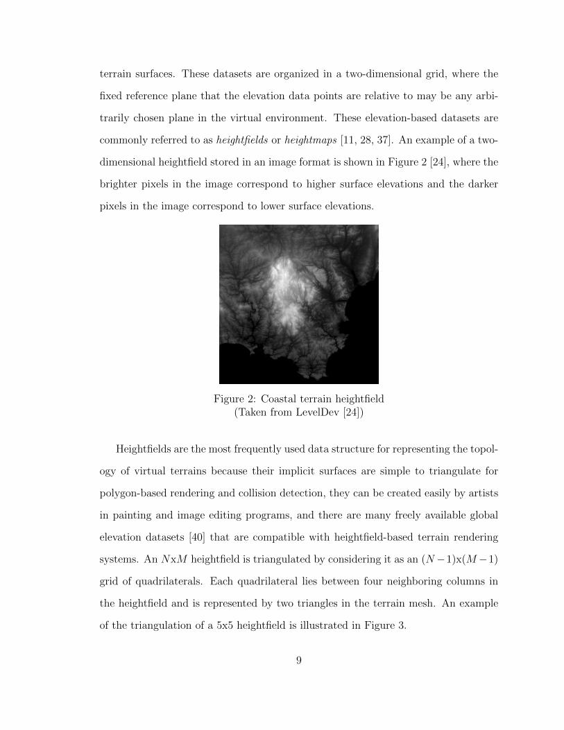
commonly referred to as heightfields or heightmaps [11, 28, 37]. An example of a two-
dimensional heightfield stored in an image format is shown in Figure 2 [24], where the
brighter pixels in the image correspond to higher surface elevations and the darker
pixels in the image correspond to lower surface elevations.
Figure 2: Coastal terrain heightfield(Taken from LevelDev [24])
Heightfields are the most frequently used data structure for representing the topol-
ogy of virtual terrains because their implicit surfaces are simple to triangulate for
polygon-based rendering and collision detection, they can be created easily by artists
in painting and image editing programs, and there are many freely available global
elevation datasets [40] that are compatible with heightfield-based terrain rendering
systems. An NxM heightfield is triangulated by considering it as an (N−1)x(M−1)
grid of quadrilaterals. Each quadrilateral lies between four neighboring columns in
the heightfield and is represented by two triangles in the terrain mesh. An example
of the triangulation of a 5x5 heightfield is illustrated in Figure 3.
9

Figure 3: Heightfield triangulation
In addition to modeling static terrain surfaces, heightfields are used extensively in
the computer graphics field to simulate dynamic terrain landscapes [1, 18, 26, 38, 41]
and large bodies of water, such as oceans and lakes [8, 20, 39]. In simulations of
dynamic terrains, heightfields represent the state of a deformable terrain surface,
typically composed of soft materials such as sand or soil, at a particular point in
time. These types of heightfields are commonly referred to as dynamically displaced
heightmaps (DDHM s) because the topological data in the heightmap is subject to
change during the game, simulation, or animation. These changes are influenced by
the actions of the players, rigid objects, and deformers, and by natural phenomenon
such as soil erosion [31] and soil slippage [6, 9].
Sumner et al. [38] and Li et al. [26] developed models of soil based solely on dy-
namically displaced heightmaps. Sumner et al. approached the problem of modeling
the creation of subtle deformations, such as footprints and tire tracks, on soft, virtual
landscapes composed of sand, soil, and mud [38]. In their approach, deformations are
created on the surfaces of heightfield-based landscapes where an overlap is detected
10

between the soil and an animated character or rigid body model. The overlapped
quantities of soil are either compacted downwards, based on a compaction ratio asso-
ciated with the soil, or transferred horizontally to the nearest column of the heightfield
that is not overlapped by any rigid body models or characters. A soil slippage algo-
rithm is applied to the soil grid to reduce the angles of the steep slopes created as a
result of soil displacements. This soil slippage algorithm identifies the columns in the
heightfield that form steep slopes with neighboring columns. Soil is transferred down-
wards along these slopes until the angles of the slopes are less than an empirically
chosen threshold. While this algorithm is sufficient for producing subtle deformations
on virtual terrain surfaces, it is not suited for simulating larger scale deformations
because it is based on a heuristic approach with empirically derived constants rather
than the physics of soil movement. Li et al. proposed a physics-based soil slippage
algorithm for heightfield-based representations of soil [26]. In their approach, the sta-
bility of a sloped configuration of soil is analyzed based on the Mohr-Coulomb failure
criterion [9]. The forces acting on an unstable configuration of soil are calculated and
used to displace quantities of sliding soil in a dynamically displaced heightmap. This
soil slippage model is described in more detail in Section 2.1.2.
Heightfields are well-suited for modeling the shape, layout, and topology of soils
piled on the ground, but, they are not able to represent quantities of loose, poured, or
falling soil. These types of soils are typically introduced in interactive simulations of
dynamic soils as a result of soil-tool interactions during excavation. For example, the
soil contained in the bucket of a simulated excavator must eventually be poured out
of the bucket to make room for new soil and to allow for further digging. When soil is
poured out of a bucket, it enters the falling state. While in this state, the soil is not
in contact with the ground or any other rigid object, and it is influenced by gravity.
Because quantities of loose, poured, and falling soil are not resting on the ground or
11

another rigid object, the surfaces of these types of soils cannot be described by an
elevation-based data structure such as a heightfield. Alternative data structures must
be used to model these types of soils in computer graphics applications.
Because soils are a type of granular material, the shape, size, and layout of a
quantity of soil can be described according to the positions, sizes, and shapes of
the individual grains that compose the soil. In the field of computer graphics, this
type of representation is commonly referred to as a particle-based representation, a
particle-system, or a discrete element method (DEM ) of simulation. Particle-based
representations of granular materials are often desired in physical simulations because
the topologies of the simulated materials are able to evolve naturally and freely based
on interparticle interactions [3]. These interparticle interactions cannot be modeled in
grid and mesh-based representations because the conceptual particles of the material
are grouped together into a numeric quantity in each grid cell. However, due to
memory and processing time constraints, it is not feasible to simulate all of the grains
in extremely fine-grained materials such as sand and soil. Instead, the simulated
particles typically represent discrete elements that are fewer in number, and therefore
larger in size, than the actual grains of the material.
Bell et al. developed a particle-based simulation of granular materials that is repre-
sented by a large system of rigid, non-spherical grains [3]. The shape and size of each
grain in their simulation is modeled as a composition of smaller, spherical particles
that are constrained together during displacement. Two examples of non-spherical
soil grains used in their approach are illustrated in 2D in Figure 4. These grains
exhibit sticking and slipping behaviors when they come into contact with each other
due to the concave features on their non-spherical bodies. These stick-slip behaviors
cause the resulting simulation to produce natural-looking angles of repose that are
claimed to be consistent with experimental results for the type of material being sim-
12

ulated. However, this approach is not suited to real-time applications because a very
large number of particles are required to achieve a realistic simulation of moderately
sized bodies of granular materials. As an example, while simulating an hourglass con-
taining approximately 100, 000 spherical sand particles, their system took an average
of 3.18 minutes to render a single frame of animation [3].
(a) (b)
Figure 4: Non-spherical soil particles
Zhu et al. developed a simulation of sand that follows particle-based fluid simu-
lation techniques [42]. In their approach, the particle-in-cell (PIC ) [17] and fluid-
implicit-particle (FLIP) [4] methods are extended to simulate the frictional and co-
hesive characteristics of extremely fine-grained materials. The PIC method simulates
the compressible flow of a fluid by tracking the motion of particles through a three-
dimensional grid. The fluid variables at each grid cell are calculated each time step by
performing a weighted averaging of nearby particle values. The FLIP method extends
and improves the PIC method to reduce the numerical dissipation that is caused by
repeatedly averaging and interpolating particle values over time. The FLIP method
achieves this by using the particles as the fundamental representation of the fluid, and
not the grid [42]. The method of Zhu et al. is a hybrid, three-dimensional grid and
particle-based approach that is computationally expensive and not suited to real-time
applications.
Other hybrid representations of soils have been developed that combine multiple
13

techniques for representing soils in real-time computer graphics applications. Holz et
al. proposed one such method that uses dynamically displaced heightmaps to repre-
sent the soil on the ground in its generally static state and particle-based methods to
represent the soil above the ground in its highly dynamic state [18]. In this approach,
spherical soil particles are generated above the surface of the ground in all locations
where rigid objects are detected to be carving over or pushing through the ground in a
horizontal manner. The generated soil particles are merged back into the soil grid on
the ground when they settle into a state of static equilibrium. The hybrid approach of
Holz et al. significantly reduces the number of particles required to achieve a realistic
simulation because large scale features are modeled with the efficient heightfield-based
method, while small scale, highly dynamic features are modeled with the better-suited
particle-based approach. Furthermore, the authors present an adaptive soil sampling
method that further reduces the number particles in the simulation. This adaptive
soil sampling method temporarily combines groups of particles that have strongly
synchronized movements into a single constrained particle. While this hybrid ap-
proach is suited for real-time simulations, it is computationally expensive to perform
mass conserving transformations between the heightfield-based representation of soil
and the particle-based representation of soil. Additionally, a separate dynamically
displaced heightfield is required for each rigid surface in the simulation that is capa-
ble of supporting mounds of piled soil. Therefore, complex simulations with many
rigid objects require many dynamically displaced heightfield data structures. Each
additional heightfield introduces a penalty on the overall performance of the simu-
lation because additional generation, collision detection, and merging operations are
required.
Onoue et al. [32] proposed another hybrid approach that continues the work done
by Sumner et al. [38]. In their approach, a two-dimensional dynamically displaced
14

heightmap is used to represent the ground soil, a spherical particle-system is used
to represent the loose, poured, and falling soil, and a multi-level, height-based data
structure is used to represent the surface of the soil piled on top of concave poly-
hedrons. This multi-level, height-based data structure is a two-dimensional grid of
stacked height spans, where each height span represents the vertical span of a rigid
object or piled soil in a column of the grid. The authors refer to this multi-level data
structure as a height span map. A 2D example of a height span map is illustrated in
Figure 5.
Figure 5: Height span map
A height span in a column of a height span map is defined by its top and bottom
points, where these points are recorded as height values relative to the bottom of
the column. A height span map is capable of representing separate quantities of soil
piled on different parts of a 3D object. Onoue et al. adapted the soil model proposed
by Sumner et al. to facilitate the compaction and subtle deformation of ground soils
based on overlaps with the rigid body height spans in a height span map.
2.1.2 Soil Slippage
Soil-covered slopes are subject to slope instability and slope failure under certain
15

conditions [6, 9, 31]. These conditions are related to the forces that are imposed on
sloped quantities of soil due to gravity, friction, and cohesion. The gravitational force
exerted on any object resting on an inclined plane is separated into two components,
one component that is perpendicular to the slope, denoted by ~g⊥, and one that is
parallel to the slope [15], denoted by ~g‖. The decomposition of the gravitational force
acting on a body of soil resting on an inclined plane is illustrated in Figure 6.
Figure 6: Soil on an incline (original in color)(Adapted from Giancoli [15])
The component of the gravitational force that is parallel to the slope, denoted by ~g‖,
is referred to as the shear stress force. The frictional force opposing the shear stress
force, denoted by ~Ff , is referred to as the shear strength force. The shear stress and
shear strength forces are the only forces contributing to the movement of soil because
the magnitude of the normal force, denoted by ~FN , is equivalent to the magnitude
of ~g⊥. In the case of soil slippage, the inclined surface supporting a sliding quantity
of soil is the surface of another quantity of soil that is in equilibrium. Therefore, the
frictional force, ~Ff , is related to the internal friction and cohesion properties of the
soil being simulated. Soil slippage does not occur along a slope unless the magnitude
of the shear stress force is greater than the magnitude of the shear strength force. By
determining whether or not this condition holds, the stability of a soil-covered slope
may be analyzed.
16

Li et al. proposed a physics-based soil slippage algorithm for heightfield-based soils
[26]. In their approach, the heightfield representing the soil is divided into rows of soil
columns, where the two-dimensional quantity of soil between a pair of neighboring
columns is referred to as a soil slice. The area of each soil slice is split into two parts, a
triangular area at the top and a rectangular area at the bottom. The triangular areas
at the top are candidate for soil slippage and the rectangular areas at the bottom are
in static equilibrium. The stability of the slope in a particular slice is analyzed by
considering only the slope of the triangular area at the top of the slice. An example
of a row of soil columns in a heightfield is illustrated in Figure 7. In this example,
there are 11 soil columns in the row and 10 soil slices between the columns.
Figure 7: Soil slices in a heightfield
Li et al. denote the shear stress and shear strength forces acting on a quantity of
soil above an arbitrary inclined plane by τ and s, respectively [26]. Shown in Figure 8
is a free body diagram of the triangular area of soil at the top of a slice [26]. In this
diagram, W represents the weight of the soil wedge resting above the inclined plane
denoted by the angle θ and the length L. The rise and run of the slope are denoted
by h and ∆x, respectively. In a heightfield-based approach, ∆x corresponds to the
distance between two neighboring soil columns and h corresponds to the difference in
17

their heights.
Figure 8: Free body diagram of sloped soil(Adapted from Li et al. [26])
An inclined plane that is supporting a quantity of soil is a failure plane if the
soil quantity above the plane will inevitably experience soil slippage [6, 9]. Li et al.
analyze the stability of the slope in the triangular area of a soil slice by evaluating the
ratio between the magnitude of the shear stress and shear strength forces [26]. This
ratio is referred to as the factor of safety [6, 9], denoted by F , and its evaluation is
given in Equation 1.
F =s
τ=cL+W cos(θ) tan(φ)
W sin(θ)(1)
In this equation, c and φ are constants that denote the coefficient of cohesion and
the angle of internal friction, respectively, of the type of soil that is being simulated.
The coefficient of cohesion is measured in ton-force per meter (t/m), where one ton-
force is approximately 9.8kN . The angle of internal friction is measured in radians.
Because L and W depend on the angle of the inclined plane, denoted by θ, they are
calculated based on θ, as shown in Equations 2 and 3. In Equation 2, γ denotes the
specific weight, which is the weight per unit area, of the soil being simulated [2]. The
specific weight is measured in ton-force per unit area (t/m2).
18

W =(h− tan(θ)∆x)∆xγ
2(2)
L =√
∆x2 + tan2(θ)∆x2 (3)
By evaluating the factor of safety using Equation 1, an arbitrary inclined plane,
denoted by θ, can be tested for failure. If F < 1 for the plane, then the soil above the
plane is unstable and will inevitably experience soil slippage. If F ≥ 1 for all inclined
planes in the sloped soil, which are the planes in the range [0, tan−1( h∆x
)], then the
sloped soil in the slice is stable. However, it is normally not desired to test arbitrary
inclined planes for failure with this method. Instead, it is desirable to calculate the
angle of the failure plane in a soil slice, if one exists, for a given configuration of
sloped soil, i.e. for any combination of h, ∆x, c, φ, and γ. To calculate the angle of
the failure plane in a slice, Li et al. solve for θ in Equation 4 [26].
F =s
τ=cL+W cos(θ) tan(φ)
W sin(θ)= 1 (4)
If a solution for θ exists and it is in the range [0, tan−1( h∆x
)], θ is the angle of the failure
plane that separates the sliding wedge of soil from the static soil in the triangular
area at the top of a slice.
To approximate the magnitude of the net force, denoted by f , acting on a wedge
of sliding soil above a determined failure plane, Li et al. divide the wedge into smaller
segments, referred to as dovetails, as shown in Figure 9a [26]. The wedge is divided
into a set of n dovetails, where the height of each dovetail, denoted by ∆h, is the
same. The ith dovetail in the wedge is the area defined by the points hi, hi−1, and b.
The forces exerted on the ith dovetail are shown in the free body diagram in Figure 9b.
19

(a) Set of dovetails (b) Single dovetail
Figure 9: Free body diagram of a dovetail(Adapted from Li et al. [26])
In this diagram, τi and si denote the shear stress and shear strength forces, respec-
tively, Ni and N ′i denote the normal forces exerted on dovetails i − 1 and i + 1,
respectively, and s′i is the equal and opposite force to the shear strength force experi-
enced by dovetail i+1. The net force acting on the wedge of soil above the determined
failure plane, denoted by f , is approximated as the sum of all of these forces across
all dovetails. This calculation is shown in Equation 5 [26].
f =n∑i=1
(τi + si + s′i +Ni +N ′i) (5)
For neighboring dovetails i and i−1, the normal forces between them, denoted by
Ni and N ′i−1, have the same magnitude, but opposite directions. That is, Ni = −N ′i−1
for i = 2, .., n. The topmost dovetail does not support any mass of soil, so it is known
that N ′n = 0. For these reasons, the sum of the normal forces across all dovetails
is reduced to N1. Similarly, the shear stress forces between any two neighboring
dovetails, denoted by si and s′i−1, have a sum of 0. That is, si = −s′i−1 for i = 2, .., n.
It is known that s′n = 0 because the top dovetail in the wedge does not support any
mass of sliding soil. Therefore, the sum of the shear strength forces across all dovetails
is reduced to s1. Using this knowledge, Equation 5 can be simplified, as shown in
20

Equation 6.
f = N1 + s1 +n∑i=1
τi (6)
Because N1 is canceled by the opposing normal force of the static soil supporting the
wedge, it is considered to be equal to 0. Furthermore, it is known that τ1 + s1 = 0
because τ1 and s1 are parallel to the failure plane. Shown in Equation 7 is a simplified
version of Equation 6 that takes these cancellations into consideration [26].
f =n∑i=2
τi (7)
For increased accuracy, Li et al. derive Equation 8 from Equation 7 by letting ∆h
tend zero [26]. That is, Equation 8 is used to calculate the net force acting on a wedge
of sliding soil where the conceptual dovetails in the wedge are infinitesimal.
f =γ∆x2
4ln
h2 + ∆x2
(tan(θ)∆x)2 + ∆x2cos(θ) +
γ∆x
2(h− tan(θ)∆x−∆x(tan−1(
h
∆x)− θ)) sin(θ)
(8)
The velocity of the sliding soil is recorded for each slice of the heightfield [26]. The
magnitude of this velocity, denoted by v, is updated each time step using the Euler
integration method shown in Equation 9.
v′ = v +f
W∆t (9)
In this equation, v and v′ are the magnitudes of the sliding soil’s velocity at the
beginning and end of the time step, respectively. The duration of the time step is
given by ∆t. The magnitude of the sliding soil’s velocity at the end of the time
21

step, denoted by v′, is equivalent to the magnitude of the sliding soil’s velocity at the
beginning of the next time step.
The height of a wedge of sliding soil in a slice is given by h− tan(θ)∆x, where θ is
the angle of the failure plane in a slice, and h and ∆x are the rise and run, respectively,
of the slope. Because the direction of the sliding wedge’s velocity, denoted by v, is
perpendicular to the soil columns, the fraction of the sliding wedge’s height that is
transferred from a higher column to a lower one over an interval of time is given by
v∆t/∆x. That is, the height that is removed from a higher column and added to a
lower one is calculated with Equation 10.
∆h =(h− tan(θ)∆x)v∆t
∆x(10)
2.2 Voxel-Based Terrain Rendering
In this section, we provide an overview of several voxel-based terrain rendering
techniques and algorithms that are well suited for real-time computer graphics ap-
plications. In the first subsection, we define the concept of a voxel and describe how
sets of voxels are used to model complex virtual terrain surfaces. In the second sub-
section, we describe methods for procedurally generating complex terrain surfaces in
a voxel-based approach. In the third subsection, we review an algorithm for extract-
ing a renderable triangular mesh corresponding to the implicit terrain surface in a
voxel-based representation.
2.2.1 Terrain Representation
A regular three-dimensional grid that divides a cubic volume of virtual space into
discrete elements is referred to as a volumetric grid, voxel grid, or voxel map [19, 23].
In computer graphics, the discrete volume elements in this three-dimensional grid are
22

referred to as voxels due to their similarity with pixels, which are picture elements,
and texels, which are texture elements. The shape, layout, and topology of a voxel-
based terrain is typically represented through the encoding of a signed or unsigned
density field in a voxel grid [14, 22, 23]. In this approach, the density of the terrain is
sampled at each of the corner points, which are referred to as sample points, on the
voxels in the grid. In the signed density approach, the sign of each density value is
used to indicate whether the respective sample point is located inside or outside the
solid terrain [14, 23]. In the typical implementation, negative density values indicate
that the point is inside the terrain and positive density values indicate that the point
is outside the terrain. The surface of the terrain is defined as the set of points in
the voxel grid where the encoded signed density field has an interpolated density
value equal to 0. Surfaces that are represented by a set of points sharing a common
value through a three-dimensional space are commonly referred to as isosurfaces.
A two-dimensional example of an isosurface represented by a signed density field is
illustrated in Figure 10.
Figure 10: Terrain isosurface in a signed density field
In the unsigned density approach, density values typically range from 0 to D,
23

where D is the maximum density of terrain that can exist at a particular sample point.
A surface threshold value, denoted by S, is chosen in the range [0, D] to indicate the
set of points in the voxel grid which define the isosurface of the terrain. This surface
threshold value is also referred to as an isovalue, and it is equivalent to the 0 value in
the signed density approach. In the typical implementation, sample points with an
unsigned density value in the range [S,D] are considered to be inside the terrain and
those with a density value in the range [0, S) are considered to be outside the terrain
[22]. To provide an even distribution of density values, S is typically chosen to be the
midpoint between 0 and D, given by D/2.
2.2.2 Terrain Generation
Voxel-based representations of terrain are capable of modeling complex, three-
dimensional surface features such as overhangs, caves, arches, and tunnels. However,
it is difficult for artists and developers to produce voxel maps manually due to their
three-dimensional nature. Instead, voxel maps are typically generated procedurally
with functions, known as density functions, that vary over a three-dimensional domain
[14]. These density functions typically employ coherent noise, such as Perlin noise,
Voronoi noise, or value noise, to facilitate the generation of randomized, natural-
looking terrain surface features. The occurrence, size, and shape of these randomly
generated surface features can be controlled by adjusting the amplitude, frequency,
persistence, and number of octaves of the noise in the density function. In fact, density
functions can be tailored to produce voxel maps for static terrains with a wide range
of topologies. Geiss demonstrated this variety by providing a set of density functions
that can be used to produce surreal-looking 3D terrains, natural-looking terrains,
spherical planets, underground tunnels, caverns, terraces, shelves, arches, and more
[14]. A few examples of terrains generated by Geiss are shown in Figure 11 [14].
24

(a) (b)
(c) (d)
Figure 11: Procedural terrains (original in color)(Taken from Geiss [14])
2.2.3 Terrain Visualization
Volume rendering is concerned with the graphical visualization of discrete three-
dimensional datasets [13, 19, 25, 27]. Volume rendering techniques are divided into
two main categories: direct volume rendering techniques and indirect volume ren-
dering techniques. In a direct volume rendering technique, an image, or rendering,
of a volumetric dataset is produced by transforming projected density values into
optical properties such as color and opacity [13, 19, 25]. That is, direct volume ren-
dering techniques generate visualizations of three-dimensional datasets directly from
density data. In an indirect volume rendering technique, an implicit isosurface is
extracted from the volumetric data and represented in the form of a geometric mesh
[27]. This mesh is rendered independently from the volumetric data using traditional
polygon-based rendering techniques.
Direct volume rendering techniques typically use a ray-traced approach to project
three-dimensional datasets onto a two-dimensional image plane. In this approach,
25

a ray is cast into the three-dimensional space through each pixel on the rendering
camera’s image plane. The three-dimensional dataset is repeatedly sampled along
each of these rays until the ray intersects with a solid object in the volume, or until
the ray escapes the volume without any intersections. If an intersection is found,
the pixel on the image plane that the ray passes through is shaded based on the
density of the intersected surface. While this method is capable of producing high
quality visualizations of volumetric data, it is not suited for rendering voxel-based
terrain surfaces in real-time applications because it is too expensive computationally
to perform repeated samples of the voxel grid along the rays that are cast.
Indirect volume rendering techniques are the preferred method for visualizing
voxel-based terrain surfaces [14, 23] because the extracted terrain mesh can be ren-
dered in real-time. The most common indirect volume rendering technique used for
voxel-based terrain is the Marching Cubes algorithm [27]. In this algorithm, a ge-
ometric mesh representing the terrain surface is extracted from the voxel grid by
independently triangulating the implicit isosurface contained in the cubic space of
each voxel. An example Marching Cubes voxel in a signed density grid is shown in
Figure 12.
Figure 12: Marching Cubes voxel
26

The set of points on the isosurface that intersect with the edges of a voxel define
the vertices of the surface mesh in that voxel. These intersection points occur on all
voxel edges that connect a sample point that is inside the terrain to a sample point
that is outside the terrain. In this thesis, we refer to these voxel edges as surface edges.
The position of the surface intersection point on each of these edges is determined
using an interpolation method, such as linear interpolation or cosine interpolation,
to determine where along the edge the density field is equal to the surface threshold
value. Recall from Section 2.2.1 that the surface threshold value S is given by D/2 in
the unsigned density approach and by 0 in the signed density approach. The formula
for calculating the position of a vertex on a surface edge with the linear interpolation
method is given in Equation 11.
x = x1 +S − ρ1
ρ2 − ρ1
· (x2 − x1) (11)
In this equation, x1 and x2 represent the positions of the two connected sample points
on the surface edge and ρ1 and ρ2 denote the densities at x1 and x2, respectively. The
positions of the surface vertices that are created on the edges of the signed density
voxel shown in Figure 12, when Equation 11 is used, are shown in Figure 13.
Figure 13: Marching Cubes voxel with surface vertices (original in color)
27

Note that it is not yet clear how these surface vertices should be connected to one
another to form a polygonal mesh representing the isosurface inside the voxel.
Because there are 8 sample points per voxel, one on each corner point, and each
sample point is either considered inside or outside the solid terrain being triangulated,
there are a total of 28 = 256 different configurations of a Marching Cubes voxel
with respect to the inside-outside relation. These 256 different configurations are
enumerated with a single byte, where the nth bit of the byte is set to 1 if and only
if the nth sample point on the Marching Cubes voxel is greater than or equal to the
surface threshold value. A look-up table indexed by these byte values is used to define
the set of triangles that should be generated from the interpolated surface vertices
in order to represent the isosurface contained within the voxel. This look-up table
is designed such that the complete set of triangles generated in a voxel grid form a
seamless triangular mesh of the isosurface encoded in that grid.
Because many of the 256 different voxel configurations can be considered a mir-
rored, inversed, or symmetric version of another configuration, the number of configu-
rations which yield a unique triangulation of a voxel in the Marching Cubes algorithm
is reducible to 15 distinct classes, which are referred to as equivalence classes [23].
Figure 14: Marching Cubes equivalence classes(Taken from Geiss [14])
28

The 14 of these 15 equivalence classes that result in the generation of at least one
triangle are shown in Figure 14 [14]. The triangles that are generated by the Marching
Cubes algorithm in the signed density voxel shown in Figure 12 are shown in Figure 15.
Figure 15: Triangulated Marching Cubes voxel
2.2.4 Terrain Level of Detail
Level of detail (LOD) algorithms are often employed to increase the efficiency of
rendering virtual terrain surfaces. These algorithms increase efficiency by adaptively
reducing the number of triangles that are rendered for sections of terrain that have less
visual importance when projected on the screen [11, 14, 23, 28, 37]. The importance
of a terrain surface in a rendered image is typically reduced proportionally with its
distance from the rendering camera due to perspective projection, occlusion, blurring,
and fog. By rendering distant sections of terrain with fewer triangles, the rendering
workload on the GPU is reduced, because fewer vertices are processed, and the change
in visual quality for the player is relatively small. However, naıvely triangulating a
continuous terrain surface at various resolutions causes cracks, or holes, to be created
in the resulting terrain mesh. These cracks occur along the edges that connect two
sections of terrain that are triangulated at different resolutions, as shown in Figure 16.
29

Figure 16: Cracks in a multi-resolution mesh
Most level of detail algorithms specify strategies for covering, hiding, or filling these
cracks with specialized geometric meshes. Shown in Figures 17 and 18 are two exam-
ples of crack filling strategies for level of detail terrain meshes.
Figure 17: Filled cracks in a multi-resolution mesh
Figure 18: Stitched cracks in a multi-resolution mesh
The first strategy, shown in Figure 17, generates additional triangles to fill the cracks
in the mesh. The second strategy, shown in Figure 18, replaces the triangles that lie
on the edge of the higher detail mesh with specialized triangles that stitch the higher
and lower detail meshes together.
Level of detail algorithms have been developed for Marching Cubes terrains by
Geiss and Lengyel [14, 23]. In their approaches, the voxel grid is partitioned into a
set of cubic sections that are referred to as terrain blocks. A voxel grid consisting of
eight terrain blocks is shown in Figure 19.
30

Figure 19: Terrain blocks (original in color)
A terrain block contains at least two voxels on each of its dimensions. Each terrain
block is adaptively assigned a level of detail based on its distance from the camera.
At each lower level of detail, a terrain block’s resolution is halved on each dimension.
As an example, Geiss partitions terrain voxel grids into sets of 32x32x32 terrain
blocks [14]. In this approach, a terrain block that is one level of detail lower than
the maximum has a resolution of 16x16x16. Furthermore, a terrain block that is two
levels of detail lower than the maximum has a resolution of 8x8x8. The minimum
resolution of a terrain block is 2x2x2. Regardless of a terrain block’s resolution, it
always encompasses the same volume of three-dimensional space in the grid. That
is, the voxels in lower detail terrain blocks are increased in size such that they fill
the entire space of their respective block. By reducing the number of voxels and
increasing their size in lower detail terrain blocks, the triangles generated are fewer
in number and larger in size. Therefore, lower detail terrain blocks are more efficient
to render than higher detail terrain blocks. A voxel grid consisting of eight terrain
blocks with varying levels of detail is shown in Figure 20.
As mentioned, naıvely extracting a terrain mesh from a multi-resolution voxel grid
with the Marching Cubes algorithm produces a mesh that contains cracks between
higher and lower detail terrain blocks. Lengyel proposed an algorithm, called the
31

Figure 20: Level of detail terrain blocks (original in color)
Transvoxel algorithm, that generates geometric stitches to fill these cracks [23]. This
algorithm requires that the level of detail of a terrain block differs by no more than
one from the level of detail of any of its neighboring terrain blocks.
The Transvoxel algorithm uses a look-up table, in addition to the Marching Cubes
look-up table, to define the triangulation of transition cells, which are voxels in lower
detail terrain blocks that border terrain blocks that are one level of detail higher.
In a transition cell, the frequency of density sample points is doubled on any face
adjacent to a higher resolution terrain block. The faces adjacent to a higher detail
terrain block are referred to as full resolution faces. The three possible configurations
of a transition cell are illustrated in Figure 21.
(a) (b) (c)
Figure 21: Transvoxel transition cells(Adapted from Lengyel [23])
In this example, the illustrated transition cells, from left to right, have one, two, and
32

three full resolution faces. In this algorithm, it is assumed that voxels border at most
one neighboring block on each dimension. Therefore, transition cells with four, five,
and six full-resolution faces are not considered.
As Lengyel argues, the number of classifications of triangulations is substantially
large for transition cells [23]. For example, a transition cell with one full resolution
face has a total of 213 = 8, 192 unique cases, a transition cell with two full resolution
faces has a total of 217 = 131, 072 unique cases, and a transition cell with three full
resolution faces has a total of 220 = 1, 048, 576 unique cases. Ideally, the number
of unique triangulation cases for any transition cell should be on the same order of
magnitude as the number of cases in the Marching Cubes algorithm [23]. To achieve
this, Lengyel first reduces the number of distinct triangulation cases for the transition
cell with a single full resolution face by dividing it into two smaller cells, as shown in
Figure 22 [23].
(a)
(b) (c)
Figure 22: Divided transition cell (original in color)(Adapted from Lengyel [23])
The portion of the divided transition cell that contains the full resolution face, shown
33

in Figure 22b, is composed of 9 unique sample points resulting in 29 = 512 cases. The
portion of the divided transition cell not containing the full resolution face, shown
in Figure 22c, is composed of 8 unique sample points and can be treated similarly
to a Marching Cubes voxel. The Transvoxel algorithm provides a look-up table that
defines the 512 triangulations of the portion of a divided transition cell that contains
the full resolution face [23]. The portion of the divided transition cell that does
not contain the full resolution face is triangulated normally with the conventional
Marching Cubes algorithm.
The number of unique cases for a transition cell with two full resolution faces is
reduced by dividing the cell into three parts, as shown in Figure 23.
Figure 23: Corner transition cell(Adapted from Lengyel [23])
Figure 23 shows a top-down view of the division of a transition cell that borders two
higher resolution terrain blocks. In this case, the two divided cells that are adjacent to
a higher resolution terrain block no longer have a cubic shape. However, these two cells
are not triangulated any differently from the cubic cell shown in Figure 22b. Their
resulting meshes are transformed after triangulation such that they fit seamlessly
inside their non-cubic cells. The method used to triangulate a transition cell with
34

three full resolution faces is an analogous extension of the method used to triangulate
a transition cell with two full resolution faces. However, transition cells with three
full resolution faces are divided into four separate cells, where three of the cells are
adjacent to a higher resolution terrain block and one of the cells is similar to a
Marching Cubes voxel.
2.3 Voxel-Based Fluid Simulation
In this thesis, we are concerned with the displacement of soil properties in a voxel
grid that consists of velocities. A relevant mathematical formulation that performs the
appropriate displacements has been devised for voxel-based fluid simulators. Voxel
grids are used in physics-based simulations of fluids, such as water, clouds, smoke, and
fire, to track the motion of a fluid through a fixed cubic volume of three-dimensional
space [5, 36]. Each voxel in the grid represents a set of fluid properties, such as
unsigned density, velocity, and temperature, that are sampled at a particular point
inside the voxel’s volume of space. The motion of a simulated fluid over time is
typically governed by the Navier-Stokes equations for incompressible flow [5, 36]. In a
voxel-based approach, a numerical solution to the Navier-Stokes equations is required
to determine the velocity of the fluid in each voxel at a particular point in time during
the simulation. The fluid properties recorded in the voxel grid are displaced based
on these velocities using an advection algorithm. We discuss advection algorithms in
the remainder of this section.
The set of velocities in a voxel grid define a three-dimensional velocity field, de-
noted by ~u, for the fluid. This velocity field is used to transport sampled fluid prop-
erties, including the velocity property itself, through the voxel grid over a discrete
time interval, denoted by ∆t [5, 36]. We denote the velocity of an arbitrary voxel
in the grid by ~ui,j,k, where i, j, and k are the indices of the voxel. The process of
35

transporting a fluid property, such as density, velocity, or temperature, through the
body of a fluid is referred to as advection. Algorithms for advecting fluid properties
in a voxel-based representation typically follow the format provided in Equation 12
[5], where qn denotes the set of values in the voxel grid for an advected property at
the beginning of the nth time step.
qn+1 = advect(~u,∆t, qn) (12)
One such advection algorithm operates by independently displacing each voxel in
the grid by its respective velocity over a given time interval [16, 33]. These displaced
voxels represent the new locations of the fluid properties at the end of the given time
interval. The fluid properties in a displaced voxel are redistributed into the overlapped
voxels in the grid based on the extent of their overlap. Shown in Figure 24 is a two-
dimensional example of the displacement of a voxel by this algorithm, where the voxel
being displaced is the center voxel with the indices i and j.
Figure 24: Displacement of a voxel (original in color)
In the example in Figure 24, the value of a fluid property in the center voxel at the
beginning of the time step, denoted by qni,j, is redistributed into the four overlapped
36

voxels that have the indices (i, j), (i+ 1, j), (i, j − 1), and (i+ 1, j − 1).
The Ω function shown in Equation 13 calculates the length of the overlap between
two voxels on one dimension, where x1 and x2 are the components of the two voxel’s
positions on that dimension.
Ω(x1, x2) = 1−min(1, |x1 − x2|) (13)
In the example in Figure 24, the fraction of qni,j that is distributed into each over-
lapped voxel is calculated with Equation 14 [16], where a and b are the indices of an
overlapped voxel and λa,b(i, j) is the fraction of the center voxel’s displaced volume
that overlaps with the voxel (a, b).
λa,b(i, j) = Ω(i+ (~ui,j)x∆t, a) · Ω(j + (~ui,j)y∆t, b) (14)
Equation 14 can be easily extended to three dimensions, as shown in Equation 15.
In this equation, a, b, and c are the indices of an overlapped voxel in the three-
dimensional grid.
λa,b,c(i, j, k) = Ω(i+ (~ui,j,k)x∆t, a) · Ω(j + (~ui,j,k)y∆t, b) · Ω(k + (~ui,j,k)z∆t, c) (15)
In this thesis, we refer to the amount of a displaced property that is transferred
into an overlapped voxel from a single displaced voxel as an inflow. The value of a
fluid property in a voxel at the end of the time step, denoted by qn+1i,j,k , is determined by
considering the combination of all inflows of that property. In the case of a spatially
additive fluid property, such as density, qn+1i,j,k is given by the sum of all inflows of that
property. This calculation is given in Equation 16, where N , M , and L denote the
37
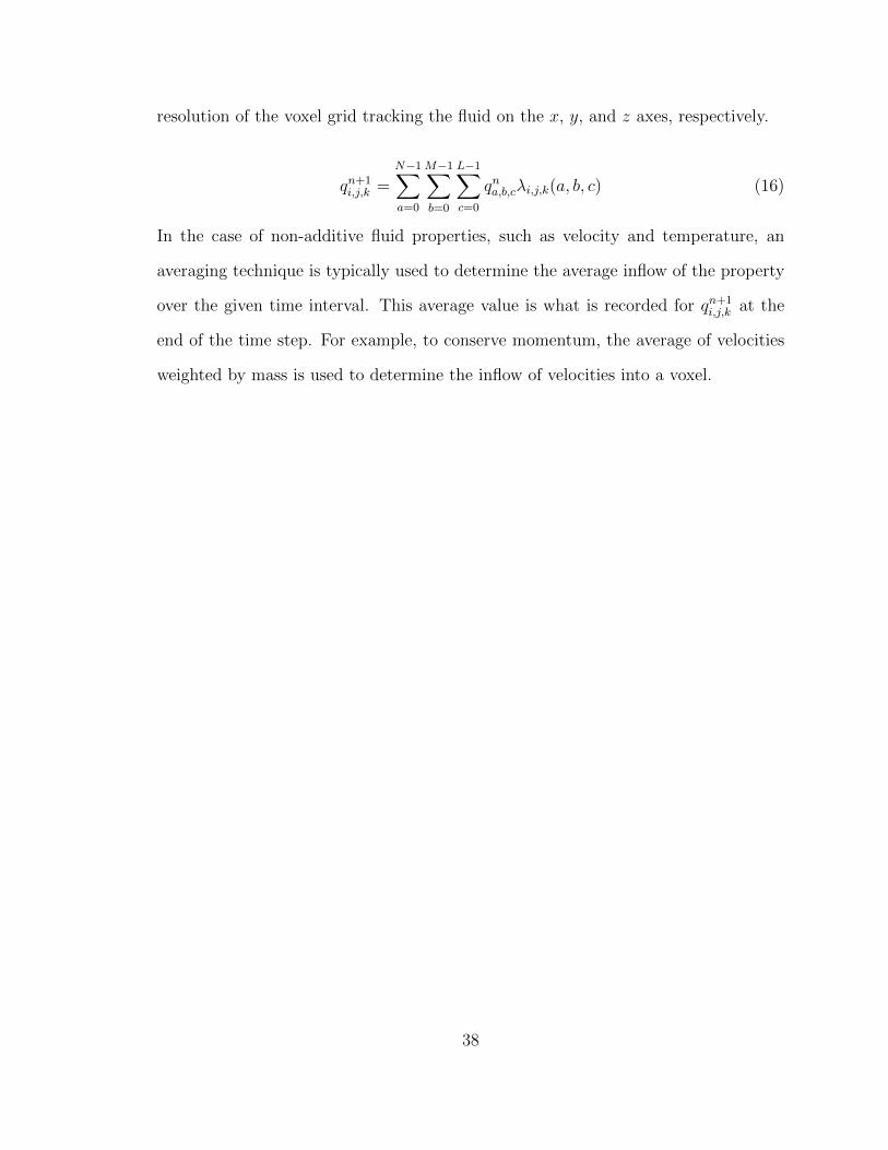
resolution of the voxel grid tracking the fluid on the x, y, and z axes, respectively.
qn+1i,j,k =
N−1∑a=0
M−1∑b=0
L−1∑c=0
qna,b,cλi,j,k(a, b, c) (16)
In the case of non-additive fluid properties, such as velocity and temperature, an
averaging technique is typically used to determine the average inflow of the property
over the given time interval. This average value is what is recorded for qn+1i,j,k at the
end of the time step. For example, to conserve momentum, the average of velocities
weighted by mass is used to determine the inflow of velocities into a voxel.
38

3 Voxel Soil
In this chapter we present a new, practical, voxel-based algorithm for simulating
sands and soils in real-time computer graphics applications. We devote a section to
each of the following: representation, simulation, visualization, and implementation.
In the first section, we describe our method of representing soil in a voxel grid. In the
second section, we present our GPU-based algorithms for simulating the physics of
soils in our voxel-based representation. In the third section, we describe the techniques
used to visualize the surfaces of the soils for a single frame of animation. In the final
section, we discuss details related to the implementation of the proposed algorithms.
3.1 Representation
In our approach, a voxel grid is used to track the motion and evolution of a simu-
lated quantity of soil in a three-dimensional space. Each voxel in this grid is described
according to the properties of the soil that is contained inside its respective volume
of space. These properties include an unsigned density value, a three-dimensional
velocity vector, and a three-dimensional force vector. For any voxel in the grid with
indices i, j, and k, the density of the soil inside the voxel is denoted by ρi,j,k, the
velocity of the contained soil is denoted by ~ui,j,k, and the direction of the force applied
on the contained soil is denoted by ~fi,j,k. In this thesis, the set of density values in
a voxel grid are referred to as a density field, the set of velocities in a voxel grid are
referred to as a velocity field, and the set of forces in a voxel grid are referred to as a
force field. The density field, velocity field, and force field are denoted by ρ, ~u, and
~f , respectively.
For simplicity, values in the density field, denoted by ρi,j,k, are recorded as fractions
of the maximum soil density that can occupy the volume of a single voxel. Recall
39

from Section 2.2.1 that, in an unsigned density approach, the maximum density of
a particular material at any given sample point in a voxel grid is denoted by D. In
our approach, the density of the soil inside an arbitrary voxel is given by ρi,j,kD.
Therefore, a voxel is considered to be completely occupied by soil if it has a value of
1.0 in the density field. Furthermore, a voxel is considered to be half occupied or one
quarter occupied by soil if it has a value of 0.5 or 0.25, respectively. An example of
a 3x3x1 slice of a density field is shown in Figure 25, where the soil inside each voxel
is visualized as though it is piled on the bottom of its containing voxel.
Figure 25: Slice of a density field
The voxel grid also tracks the positions of rigid bodies inside its three-dimensional
space. In addition to recording values related to the properties of the soil, each voxel
records an unsigned density value that represents the combined density of the rigid
bodies occupying its space. For any voxel in the grid with indices i, j, and k, the
combined density of the rigid bodies inside that voxel is denoted by ψi,j,k. The set of
rigid body density values in a voxel grid are referred to as a collision field, denoted
by ψ, and collision fields are used to detect and resolve collisions between rigid bodies
and soil during the simulation. We assume all rigid bodies in a collision field share
a uniform density, where the maximum density of rigid bodies that can occupy the
40

volume a single voxel is denoted by D2. For simplicity, the density values in the
collision field, denoted by ψi,j,k, are recorded as fractions of D2 similar to the soil
density values in ρ. An example of a combined density and collision field is shown in
Figure 26, where rigid bodies are visualized as though they are piled on the bottom
of their containing voxels and soils are visualized as though they are piled on top of
rigid bodies.
Figure 26: Slice of a density field and a collision field
The values associated with the density field, velocity field, force field, and collision
field at a particular point in time during the simulation are referred to as the state
of the simulation. The state of the simulation at the beginning of the nth time step
is denoted by βn, and the soil density, velocity, force, and rigid body density values
associated with a particular voxel in βn are denoted by ρni,j,k, ~uni,j,k,
~fni,j,k, and ψni,j,k,
respectively, where i, j, and k are the indices of the voxel. These values are collectively
denoted by βni,j,k.
The voxel volume constraint shown in Equation 17 must be satisfied for a given
state of the simulation to be physically plausible.
∀i, j, k ∈ N, 0 ≤ ρni,j,k + ψni,j,k ≤ 1 where i < N, j < M, k < L (17)
41

In this equation, N , M , and L denote the resolution of the voxel grid on the x, y, and
z axes, respectively. For the voxel volume constraint to be satisfied, each value in the
soil density field, given by ρni,j,k, must be in the range [0, 1−ψni,j,k]. If ρni,j,k > 1−ψni,j,k
for some voxel, then that voxel is occupied by more soil than it is physically capable
of containing in its available space. We refer to these types of voxels as overflowed
voxels. As we will discuss in Sections 3.2.1 and 3.2.4, overflowed voxels may exist
temporarily in our simulation due to certain constraints that are associated with a
parallel, GPU-based simulation.
3.2 Simulation
The state of the simulation evolves over time to reflect the motion of the virtual
soil in a three-dimensional space. We consider three different types of motion in our
voxel-based soil simulation: projectile motion, slippage motion, and contact motion.
Quantities of falling soil, such as poured and dumped soils, experience projectile
motion due to the downward acceleration of gravity. Quantities of piled soil, such
as the soil on the ground or in the bucket of an excavator, experience soil slippage
due to the presence of unstable slopes on their surfaces. Both falling and piled
quantities of soil experience contact motion when they are subjected to deformation
and displacement from dynamic objects and bodies.
Given the state of the simulation at the beginning of the nth time step, denoted
by βn, we determine the state of the simulation at the end of the time step, denoted
by βn+1, by applying a transformation to βn that reflects the net motion of the soil
over the given time interval. This transformation is divided into three separate trans-
formations that update the state of the simulation based on the projectile, slippage,
and contact motions of the soil. That is, βn is transformed to reflect the net motion
of the soil over a discrete time interval, denoted by ∆t, as shown in Equations 18, 19,
42

and 20.
βdef = deformation(βn,∆t) (18)
βproj = projectile(βdef ,∆t) (19)
βn+1 = slippage(βproj,∆t) (20)
In these equations, projectile, slippage, and deformation represent functions that
transform a given state of the simulation based on the projectile, slippage, and contact
motions, respectively. The intermediate states of the simulation that are produced
after the deformation and projectile transformations are denoted by βdef and βproj,
respectively.
The transformation from βn to βn+1 is split into three separate functions because
it is significantly easier to develop separate software modules that transform the state
of the simulation based on these different types of motions independently, rather than
concurrently. In our approach, we use a GPU-based advection algorithm to transform
the state of the simulation based on the projectile motion of loose, poured, and falling
soils. This algorithm is described in detail in the first and second subsections of this
section. In the third subsection, we describe a GPU-based soil slippage algorithm that
operates on our voxel-based representation of soil. Lastly, in the fourth subsection, we
describe our GPU-based algorithm for transforming the state of the simulation based
on soil-object interactions. Shown in Algorithm 1 is psuedocode that demonstrates
the high-level structure of our complete algorithm.
43
initialize simulation;
while simulation is running do
∆t = get the elapsed time since the last iteration;
displace player-controlled rigid objects based on ∆t;
ψ = construct a collision field for the rigid objects;
ρ, ~u, ~f = SoilDeformation(~f , ∆t, ρ, ~u, ~f , ψ);
ρ, ~u, ~f = SoilAdvection(~u, ∆t, ρ, ~u, ~f , ψ);
~u = ~u+ ~g∆t
ρ = SoilSlippage(ρ, ∆t, ψ);
RenderSoil(ρ);
display frame;
end
Algorithm 1: High-level algorithm for voxel-based soil simulation
We discuss the soil deformation, advection, and slippage transformations in a different
order than they are specified in Algorithm 1. We discuss these transformations in
the order that we recommend they be implemented based on their complexity and
importance. The force field, ~f , is utilized in the deformation transformation and the
velocity field, ~u, is utilized in the advection transformation. These two vector fields
are discussed in more detail in their respective subsections.
3.2.1 Soil Advection
We utilize an advection algorithm to displace quantities of soil in a voxel grid.
Recall from Section 3.1 that the properties recorded in our voxel-based representation
are unsigned density, denoted by the density field ρ, velocity, denoted by the velocity
field ~u, direction of applied force, denoted by the force field ~f , and rigid body density,
44

denoted by the collision field ψ. In this subsection, we denote the values associated
with these fields at the beginning and end of the advection transformation by βn
and βn+1, respectively. In this subsection, βn+1 does not represent the state of the
simulation at the end of the nth time step, as it does in Section 3.2. In this subsection,
βn+1 represents the state of the simulation at the end of the advection transformation.
Following the general format of an advection algorithm, specified in Equation 12 [5],
the format of our algorithm is shown in Equation 21. That is, our advection algorithm
transforms βn into βn+1 based on the state of the velocity field over a given interval
of time. The collision field is not affected by this transformation because the motion
of rigid bodies is based on user input, animation data, or a physics engine.
βn+1 = advect(~u,∆t, βn) (21)
Our advection algorithm is designed such that the values associated with an ar-
bitrary voxel in βn+1, denoted βn+1i,j,k , can be calculated in parallel for each voxel in
the grid. This algorithm is suited to GPU implementation, where a separate thread
on the GPU is dispatched to calculate and record the value of βn+1i,j,k . Because our
algorithm is required to operate in real-time, we do not calculate the net inflow of a
particular soil property into a voxel by considering the displacement of all voxels in
the grid, as shown in Equation 16. Instead, we only consider inflows from neighboring
voxels, where a voxel is considered a neighbor of another voxel if it is adjacent to that
voxel in the grid, or if it is the same voxel. In other words, quantities of soil are only
transferred into adjacent voxels or their same voxel over the duration of a single time
step in our GPU-based advection algorithm. We choose the resolution and size of our
voxel grid such that the magnitude of any voxel’s velocity can be reasonably restricted
to not exceed the length of one voxel at any point in time during the simulation.
45
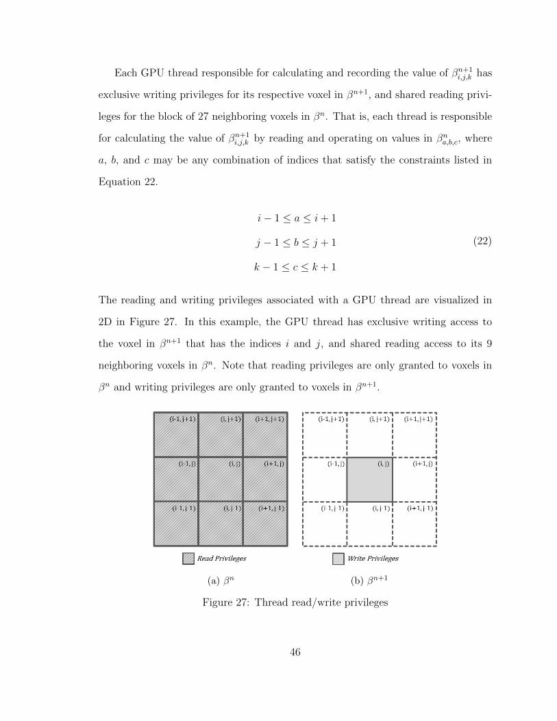
Each GPU thread responsible for calculating and recording the value of βn+1i,j,k has
exclusive writing privileges for its respective voxel in βn+1, and shared reading privi-
leges for the block of 27 neighboring voxels in βn. That is, each thread is responsible
for calculating the value of βn+1i,j,k by reading and operating on values in βna,b,c, where
a, b, and c may be any combination of indices that satisfy the constraints listed in
Equation 22.
i− 1 ≤ a ≤ i+ 1
j − 1 ≤ b ≤ j + 1
k − 1 ≤ c ≤ k + 1
(22)
The reading and writing privileges associated with a GPU thread are visualized in
2D in Figure 27. In this example, the GPU thread has exclusive writing access to
the voxel in βn+1 that has the indices i and j, and shared reading access to its 9
neighboring voxels in βn. Note that reading privileges are only granted to voxels in
βn and writing privileges are only granted to voxels in βn+1.
(a) βn (b) βn+1
Figure 27: Thread read/write privileges
46

We extend the advection algorithm described in Section 2.3 [16] to facilitate the
displacement of soil through a voxel grid based on projectile motion. In this algorithm,
all soil is considered “displaced”, even if it ends up in its original voxel. We extend this
advection algorithm by considering collisions amongst displaced soil quantities and
rigid bodies. A collision occurs when a displaced quantity of soil causes the resulting
state of the simulation to violate the voxel volume constraint, given in Equation 17.
That is, a soil-object or soil-soil collision occurs inside a voxel if the combined volume
of displaced soils and rigid bodies inside that voxel exceed its volume capacity. A
simple example of this scenario is illustrated in 2D in Figure 28. In this example, the
displaced quantity of soil in the center voxel, with indices i and j, collides with the
soil in the two neighboring voxels that have the indices (i, j − 1) and (i+ 1, j − 1).
Figure 28: Internal collision caused by displaced soil (original in color)
In this example, the density of soil that collided with the soils inside these two neigh-
boring voxels are given by ρi,jλi,j−1(i, j) and ρi,jλi+1,j−1(i, j), respectively. To satisfy
the voxel volume constraint, these collided density values must be distributed else-
where in the voxel grid such that they are placed in nearby voxels that are capable
of containing their volume.
47

The soil properties in our voxel-based representation, ρ, ~u, and ~f , are displaced
concurrently in the same operation, as shown in Equation 21, rather than indepen-
dently in separate advection operations. These properties are displaced in the same
operation because displaced soil densities may undergo motions that temporarily
deviate from the velocity field due to collisions. The velocity and force properties
associated with a density after collision must follow its new motion. In our approach,
voxels in βn are considered to be in a locked state if they are completely occupied
by soil, rigid objects, or a combination of both. In this locked state, no quantities of
soil from the surrounding 26 voxels are able to flow into the voxel over the given time
interval. Displaced quantities of soil that attempt to enter a locked voxel are simply
returned to their originating voxels as inflow with zero velocity, which we refer to as
backflow. A quantity of soil inside a locked voxel may flow out of the voxel if it has
a non-zero velocity. An example of this collision resolution technique is illustrated in
2D in Figure 29.
(a) βn (b) βn+1
Figure 29: Locked voxels
In this example, locked voxels are marked with a lock symbol. The displaced quantity
of soil that has a density value of 0.6 is returned to its originating voxel because its
outgoing soil overlaps with a locked voxel. The displaced quantity of soil that has a
48

density value of 0.8 has 75% of its density returned to its originating voxel, and 25%
of its density distributed into overlapping neighbor voxels. This is because 75% of the
displaced voxel’s volume overlaps with the originating voxel and locked voxels, and
25% of the displaced voxel’s volume overlaps with unlocked neighboring voxels. To
keep the soil contained inside the voxel grid’s cubic volume of space, we assume that
all voxels outside the grid are in a constant locked state. Therefore, any displaced soil
quantities that cross the boundaries of the voxel grid are returned to their originating
voxels as backflow.
Shown in Equation 23 is the function used to calculate the inflow of density into
a voxel with indices i, j, and k from a voxel with indices a, b, and c. In this equation,
ρna,b,c denotes the density of the soil inside the voxel (a, b, c) at the beginning of the
advection transformation, and λi,j,k(a, b, c) denotes the fraction of (a, b, c)’s displaced
volume that overlaps with the voxel (i, j, k).
inflowi,j,k(a, b, c) = ρna,b,cλi,j,k(a, b, c) (23)
Equation 24 gives the function used to calculate the density of soil that returns to
the voxel (i, j, k) as backflow when it is displaced out of (i, j, k) into another voxel
with indices (a, b, c). That is, Equation 24 calculates the density of displaced soil that
returns to its originating voxel due to the locked or unlocked state of a neighboring
voxel. In this equation, ψna,b,c denotes the density of the rigid bodies in a voxel with
indices a, b, and c. This function assumes that (i, j, k) 6= (a, b, c) because a voxel
cannot receive backflow from itself.
backflowi,j,k(a, b, c) =
0 : ρna,b,c + ψna,b,c < 1
inflowa,b,c(i, j, k) : ρna,b,c + ψna,b,c ≥ 1(24)
49

Equations 25 and 26 are used to calculate the net inflow and net backflow, respectively,
for a voxel, with indices i, j, and k, from its block of 27 neighboring voxels.
net inflow(i, j, k) =1∑
a=−1
1∑b=−1
1∑c=−1
inflowi,j,k(i+ a, j + b, k + c) (25)
net backflow(i, j, k) =1∑
a=−1
1∑b=−1
1∑c=−1
backflowi,j,k(i+ a, j + b, k + c) (26)
Shown in Equation 27 is the function used to calculate the density of soil inside a
particular voxel at the end of the advection transformation.
ρn+1i,j,k =
net inflow(i, j, k) + net backflow(i, j, k) : ρni,j,k + ψni,j,k < 1
inflowi,j,k(i, j, k) + net backflow(i, j, k) : ρni,j,k + ψni,j,k ≥ 1(27)
In this function, the inflow of density into a particular voxel is based on its locked or
unlocked state. If the voxel is in an unlocked state, the inflow of density into the voxel
is the net inflow received from all 27 neighboring voxels, calculated with Equation 25.
If the voxel is in a locked state, its net inflow of density is the inflow it receives from
itself, calculated with Equation 23. The net backflow of density is added to a voxel’s
inflow, as shown in Equation 27, regardless of its locked or unlocked state.
As discussed, displaced quantities of soil also have a velocity and force property
associated with their density. We use a weighted averaging technique to calculate
the velocity and force associated with the soil inside a particular voxel in βn+1. This
technique calculates the average velocity and force that flowed into the voxel, where
more weight is assigned to the velocities and forces that entered the voxel with larger
volumes of soil. That is, the weight assigned to each inflowing velocity and force
property is based on its associated density value. The weighted averaging of the
50

velocity property is shown in Equation 28, where ~un+1i,j,k denotes the velocity of the soil
in a voxel, with indices i, j, and k, in βn+1.
~un+1i,j,k =
m∑a=0
~u ina ρina
m∑a=0
ρina
(28)
The total number of inflowing soil quantities is given by m, and ~u ina and ρina denote the
velocity and density, respectively, of the ath inflowing quantity of soil. The weighted
averaging of the velocity property is identical to the weighted averaging of the force
property.
This advection algorithm introduces overflowed voxels in the voxel grid. Recall
from Section 3.1 that a voxel is overflowed if it is occupied by more soil than it is
physically capable of containing. That is, a voxel in the grid with the indices i, j, and
k is overflowed if ρi,j,k > 1−ψi,j,k. Unlocked voxels may overflow during this advection
algorithm if they receive a net inflow of soil from their neighboring 27 voxels that is
more soil than they are capable of containing. Ideally, the displaced quantities of
soil would collide with one another before causing any overflows in unlocked voxels.
However, because our algorithm displaces soil quantities in parallel on the GPU,
detecting and resolving these collisions in an efficient manner is a difficult task. To
avoid this, we perform an overflow resolution process on the GPU after every advection
transformation in an attempt to produce a density field that satisfies the voxel volume
constraint. Overflow resolution techniques redistribute overflowed densities in a voxel
grid based on some heuristic. Shown in Figure 30 are three examples of overflow
resolution heuristics that are well-suited for resolving overflows in our voxel-based
representation of soil.
51

Figure 30: Overflow resolution techniques
The upper square indicates the state βn and the three lower squares show the results
of applying three overflow resolution heuristics to produce βn+1.
The first heuristic distributes overflowed densities into all neighboring voxels
evenly, as shown on the left in Figure 30. The second heuristic transfers overflowed
densities upwards one voxel in the grid, as shown in the center of Figure 30. The
third heuristic transfers overflowed densities into the set of neighboring voxels that
are one level higher than the overflowed voxel, as shown on the right in Figure 30.
The density that is transferred into each of these upper voxels is determined by as-
sociating a weight with each upper voxel. In this example, the upper voxels in the
corners receive 25% of the overflow and the upper voxel in the center receives 50% of
the overflow.
The first overflow resolution heuristic is well suited to resolving overflows in falling
quantities of soil, while the second and third heuristics are well suited to resolving
overflows in piled quantities of soil. However, it is not guaranteed that a single
pass of any of these overflow resolution techniques will produce a density field that
satisfies the voxel volume constraint. A single pass is not guaranteed to resolve all
52

overflows because additional overflows may be created in neighboring voxels that
receive distributed densities. Therefore, multiple passes of an overflow resolution
algorithm are performed on the GPU to increase the probability of producing a density
field containing no overflowed voxels. In our approach, we perform 4 passes of an
overflow resolution algorithm that uses the second heuristic on the GPU after each
advection transformation.
3.2.2 Body Forces
Once per time step we transform the state of the velocity field to reflect the
acceleration of soil based on body forces, such as gravity. In our approach, we perform
this transformation immediately after each advection transformation. We calculate
the accelerated velocity of the soil inside each voxel using Euler integration. If a
particular voxel is not occupied by any soil, then the velocity associated with that
voxel is set to 0. Shown in Equation 29 is the function used to accelerate a voxel’s
velocity over a given time step based on gravity.
~un+1i,j,k =
~uni,j,k + ~g∆t : ρni,j,k 6= 0
0 : ρni,j,k = 0(29)
In this equation, ~uni,j,k and ~un+1i,j,k denote the velocity of a particular voxel, with indices i,
j, and k, before and after the body force transformation, respectively. The density of
soil occupying the voxel is denoted by ρni,j,k, ~g is a downward gravitational acceleration
vector, and ∆t is the duration of the time step.
3.2.3 Soil Slippage
Recall from Section 2.1.2 that Li et al. proposed a physics-based soil slippage al-
gorithm that operates on soil slices in a dynamically displaced heightmap [26]. We
53

use this soil slippage model to facilitate the slippage of soils in a 3D density field.
However, because the height of a piled soil column cannot be sampled directly in a
density field, we instead perform slope stability analysis and soil slippage computa-
tions on an indirect, height-based representation of the density field. The changes
made to this indirect representation are reflected in the density field after the soil
slippage model has been applied.
Once per time step, we construct a height span map that represents the state of
the density and collision fields for soil slippage computations. We refer to this height
span map as a multi-level heightfield. The multi-level heightfield is an NxL grid of
columns, where each column corresponds to a column in the voxel grid. Each column
of the multi-level heightfield is a sorted list of non-overlapping height spans, where
the height spans in a column are sorted in a bottom-up manner and are centered
in their containing voxels. The multi-level heightfield is similar to the height span
maps used by Onoue et al. [32], except it includes height spans for all rigid objects,
all soil piled on those objects, soil piled on the ground, and falling soil. Onoue et al.
used a separate height span map to record the soil piled on each rigid object. The
multi-level heightfield consists of four different types of height spans: rigid body, piled
soil, falling soil, and edge height spans.
A height span in a column of the multi-level heightfield is denoted by Hi =
Bi, Ti, µi, where i is the index of the height span in the column, Bi and Ti are
the heights of its bottom and top points, respectively, and µi is an integer that en-
codes the height span’s type. The height of a height span’s bottom and top points are
specified relative to the bottom of the column. Therefore, the local height of a height
span is given by Ti − Bi. A height span in a multi-level heightfield extends through
a non-empty set of voxels in its corresponding column of the voxel grid. The top and
bottom voxels in this set contain the top and bottom points of the height span. The
54

voxels that lie between a height span’s top and bottom voxels are referred to as inner
voxels. Shown in Figure 31 is an example of a height span and its corresponding
column of voxels in the grid. A column of voxels associated with a height span may
contain zero, one, or more inner voxels depending on the local height of the height
span. The bottom and top voxels may be the same voxel if a height span begins and
ends in that voxel.
Figure 31: Height span in a column of voxels
The set of height spans in a column of the voxel grid are constructed in bottom-up
order by searching upwards through the voxels in that column, beginning with the
bottommost voxel. At each voxel in this search, a set of conditions are evaluated
to determine if a particular type of height span begins inside the voxel. If one does
not begin, then the search continues up the column to the next voxel. If one does
begin, then the height of the height span’s bottom point is calculated. Another set
of conditions are evaluated to determine if the height span ends in that voxel. If
the height span does not end, then the search continues up the column until one of
these conditions are met and the top voxel of the height span is found. Once the top
voxel of the height span is found, the height of its top point is calculated and the
height span is recorded in the multi-level heightfield. The top voxel of the recorded
55

height span is checked for the beginning of a different type of height span. The search
continues in this manner until the topmost voxel in the column is processed.
Shown in Tables 1, 2, and 3 are the conditions which define the construction of
rigid body, piled soil, and falling soil height spans. In each table, a set of conditions are
provided for the bottom and top voxels of each type of height span. These conditions
are used during the upwards search to determine if a particular voxel contains the
bottom or top point of a height span. If there is a conflict and multiple types of
height spans are determined to begin inside a particular voxel, then priority is given
in the following order: piled soil, rigid body, falling soil.
Rigid Body Height Span
Voxel Condition Height (ω)
Top ψi,j,k < 1 and ψi,j+1,k ≥ 1 ψi,j,k
Bottom ψi,j−1,k ≥ 1 1− ψi,j,k
Table 1: Height span construction (rigid bodies)
Piled Soil Height Span
Voxel Condition Height (ω)
Top
ρi,j,k < 1− ψi,j,k and ψi,j+1,k ≥ 1 ψi,j,k + ρi,j,k
ρi,j,k < 1 and ψi,j+1,k < 1 ρi,j,k
ψi,j,k > 0 and ψi,j+1,k < 1 ρi,j,k
Bottomψi,j+1,k ≥ 1 and ψi,j,k < 1 ψi,j,k
j = M − 1 0
Table 2: Height span construction (piled soil)
56

Falling Soil Height Span
Voxel Condition Height (ω)
Topψi,j,k > 0 0
ρi,j,k < 1 0
Bottom ρi,j,k ≥ 1 and ψi,j,k = 0 0
Table 3: Height span construction (falling soil)
In Tables 1, 2, and 3, i, j, and k are the indices of the current voxel in the upwards
search. If a bottom or top condition is true for that voxel, then that voxel contains
the bottom or top point of the respective type of height span. The height of this point
relative to the bottom of the voxel is specified next to each condition. Equation 30
is used to calculate the height of the bottom or top point relative to the bottom of
the column.
B, T = M − 1− j + ω (30)
In this equation, M denotes the resolution of the voxel grid on the y-axis, j denotes
the y-index of the voxel containing the point, and ω denotes the height of the point
relative to the bottom of its containing voxel.
Simply put, Tables 1, 2, and 3 construct height spans with the following rules and
assumptions:
• The rigid bodies in the bottom voxel of a rigid body height span are distributed
at the top of the voxel.
• The rigid bodies in the top voxel of a rigid body height span are distributed on
the bottom of the voxel.
57

• The inner voxels of a rigid body height span are completely occupied by rigid
bodies.
• A rigid body height span must contain at least one inner voxel.
• A piled soil height span always starts at the bottom of the bottommost voxel
in the column.
• A piled soil height span always starts directly on top of a rigid body height
span.
• The inner voxels of a piled soil height span are completely occupied by soil.
• The top, bottom, and inner voxels of a falling soil height span are completely
occupied by soil.
• The top, bottom, and inner voxels of a falling soil height span contain no rigid
bodies.
Figure 32: Height spans in a voxel grid (original in color)
58

Shown in Figure 32 is a visual, two-dimensional example of the rigid body, piled
soil, and falling soil height spans that are constructed in the columns of a density
field and a collision field.
Two piled soil height spans in neighboring columns of the multi-level heightfield
form a soil slice if they have a positive intersection of height. The intersection of
height between two height spans is calculated using Equation 31, where Hi and Hj
are two height spans in neighboring columns.
Hi ∩Hj = min(Ti, Tj)−max(Bi, Bj) (31)
The area of a soil slice between two piled soil height spans is divided into a rectangular
and a triangular area, similar to soil slices in a heightfield-based approach [26]. The
rectangular area in a soil slice lies in the region where there is an intersection of
height between two neighboring height spans. That is, the top of the rectangular
area has a height of min(Ti, Tj) and the bottom of the rectangular area has a height
of max(Bi, Bj). The triangular area in a soil slice connects the top point of the lower
height span to the highest point on the higher height span that does not lie in the
rectangular area of the next higher slice in the column. The conceptual construction
of these soil slices is shown in Figure 33. In Figure 33a, the triangular area at the
top of the slice forms a sloped surface that connects the top points of the two height
spans. In Figure 33b, the triangular area at the top of the slice does not connect the
top points of the two height spans because the top point of the higher height span is
included in another slice. Shown in Equation 32 is the function used to calculate the
height of the triangular area at the top of a soil slice between two piled soil height
spans.
59

(a) (b)
Figure 33: Slices between two piled soil height spans
h = min(Ti, Bj+1)− Tj (32)
In this equation, Ti is the top point of the higher height span, Tj is the top point of the
lower height span, and Bj+1 is the bottom point of the next height span in the lower
height span’s column. The slope of the soil in a slice is given by h and ∆x, where
h is calculated with Equation 32 and ∆x is the horizontal distance between the two
height spans. The triangular quantities of soil at the top of each soil slice are candidate
for soil slippage. We use the soil slippage algorithm described in Section 2.1.2 [26]
to calculate the change in local height of a height span with respect to one of its
adjacent soil slices. The net change in local height of a piled soil height span is the
sum of the height changes in each of its adjacent soil slices.
Piled soil on the edge of a rigid object will not slide off the edge as it naturally
should if there are no piled soil height spans beyond the boundaries of the object to
receive the sliding soil. This problem is illustrated in Figure 34. To fix this problem,
we procedurally insert a piled soil height span that has a local height of zero next
to the bottom points of height spans that are on the edge of a rigid object. These
procedurally inserted height spans are referred to as edge height spans. If the bottom
60

point of a piled soil height span on the edge of a rigid body already has another height
span next to it, then no edge height span is inserted.
Figure 34: Missing soil slices on an edge (original in color)
Shown in Figure 35 is an example of a row of height spans, and their conceptual soil
slices, in a multi-level heightfield.
Figure 35: Soil slices in a multi-level heightfield (original in color)
In this example, an edge height span is inserted next to the bottom point of the piled
soil height span on the right edge of the rigid object. This edge height span produces
a soil slice that causes the soil to slide off the edge of the object and enter the falling
state. An edge height span is not inserted next to the bottom point of the piled soil
61

height span on the left edge of the rigid object because another height span already
occupies this space.
A change in the local height of a piled soil height span due to soil slippage is
reflected in the density field, as shown in Figure 36. In this approach, soil density is
added or removed sequentially from the top voxel of a piled soil height span based on
the height span’s net change in local height.
Figure 36: Height changes reflected in a density field
In the example in Figure 36, the net change in local height of the piled soil height
span is given to be −1.85. Therefore, 1.85 is removed from the density of soil in the
height span’s column of voxels, starting from its top voxel and continuing downwards.
If the piled soil height span is increased in height, then density is added to the height
span’s column of voxels, starting from its top voxel and continuing upwards.
3.2.4 Soil Deformation
Recall from Section 3.1 that a three-dimensional collision field encodes the loca-
tions of rigid bodies in a voxel grid. In the context of this thesis, rigid bodies are
3D game objects that influence the state of the simulated soil. Because these game
object’s movement are based on user input, animation data, or a physics engine, the
62

locations of rigid bodies in a collision field are not updated by transporting their den-
sities through the grid in a procedural manner similar to soil. Instead, the collision
field is reconstructed at the beginning of each time step, as shown in Algorithm 1, to
reflect the new positions of the rigid bodies in the grid after their displacement. That
is, the collision field is a temporary snapshot of the locations of all rigid bodies in a
voxel grid during a single time step.
The process of transforming a 3D, surface-based representation of an object, such
as a polygonal mesh, into a voxel-based representation is referred to as voxelization
[10, 12]. The collision field is reconstructed each time step by voxelizing all rigid
game objects into its voxel grid. Because 3D game objects are typically represented
in the form of a polygonal mesh, constructing a collision field directly from these
objects requires them to be voxelized based on the location and orientation of each
of their polygons. However, it is computationally expensive to voxelize large sets of
objects with highly detailed meshes in real-time applications. It is more efficient, and
much simpler, to voxelize 3D geometric primitives such as spheres, ellipsoids, cuboids,
cylinders, and cones. These objects are more efficient to voxelize because their volume
can be represented mathematically with a density function [22]. Voxelizing a 3D
object based on a density function is logically equivalent to generating voxel terrain
with a density function, as described in Section 2.2.2. In both cases, an empty voxel
grid is populated with densities by sampling and recording the value of a density
function at each voxel in the grid.
Laprairie et al. proposed a set of virtual volume sampling functions, which are 3D
density functions, for geometric primitives such as spheres, ellipsoids, cuboids, cylin-
ders, and cones [22]. In our approach, we approximate the volume of each rigid game
object with a unionized set of these geometric primitives. We are able to construct
the collision field more efficiently by voxelizing the set of geometric primitives asso-
63

ciated with each game object rather than their detailed meshes. A two-dimensional
example of the voxelization of geometric primitives is shown in Figure 37. In this
example, the volumes of two objects, denoted by O1 and O2, are voxelized to produce
the collision field in Figure 37b. The volume of O1 is approximated with two cuboid
primitives and the volume of O2 is approximated with a single sphere primitive. The
collision field in this example is visualized as though densities are distributed evenly
inside the space of their containing voxels.
(a) (b)
Figure 37: Voxelization of 3D geometric primitives (original in color)
As described in Sections 3.2.1 and 3.2.3, the collision field, denoted by ψ, is used to
detect and resolve collisions that occur when falling or sliding quantities of soil come
into contact with a rigid body. However, collisions also occur when moving rigid
bodies come into contact with soil. For example, the blade of a simulated bulldozer
may be used to push large quantities of soil along the surface, or the bucket of a
simulated excavator may be used to lift quantities of soil out of the ground. These
types of collisions occur when the voxel volume constraint, specified in Equation 17,
is violated as a result of a change in the collision field. A 2D example of this type of
64

collision is illustrated in Figure 38.
Figure 38: A moving object colliding with soil (original in color)
In this example, the change in position of the rigid body causes a collision in the three
voxels that each have a soil density value of 0.8. These voxels are in collision because
their combined density of soil and rigid objects exceeds a value of 1. The density of
the collided quantity of soil in any one of these voxels is given by ρi,j,k − (1− ψi,j,k),
where i, j, and k are the indices of a collided voxel. In this example, the density of
the collided quantity of soil in each voxel containing a collision is 0.3.
As shown in Algorithm 1, we perform a soil deformation transformation on the
voxel grid after the collision field is reconstructed each time step. This transforma-
tion pushes collided quantities of soil through the grid based on the direction of their
applied force from contacting rigid bodies. For each voxel in the grid, the direction of
the applied force associated with the collided quantity of soil in the voxel is denoted
by ~fi,j,k, where i, j, and k are the indices of the voxel. The soil deformation transfor-
mation is split into two separate GPU-based operations: force application and force
propagation.
The force application operation updates the direction of the applied force asso-
ciated with the collided soil in each voxel after the collision field is reconstructed.
65
In our approach, the direction of the force exerted on a quantity of collided soil is
assumed to be equivalent to the direction of the colliding object’s velocity. Shown in
Equation 33 is the force application function used to update the force field after the
collision field is reconstructed.
~fn+1i,j,k =
vψi,j,k
||vψi,j,k||: ρni,j,k + ψni,j,k > 1 ∧ ψni,j,k 6= 0
~fni,j,k : ρni,j,k + ψni,j,k > 1 ∧ ψni,j,k = 0
0 : ρni,j,k + ψni,j,k ≤ 1
(33)
In this equation, ~fni,j,k and ~fn+1i,j,k denote the direction of the applied force associated
with a particular voxel before and after the force application operation, respectively.
The density of the soil and rigid objects in the voxel are denoted by ρni,j,k and ψni,j,k,
respectively. The velocity of the rigid object in the voxel is denoted by vψi,j,k. Note that
only overflowed voxels have a non-zero force in the force field. If an overflowed voxel
does not contain any rigid objects, then that voxel’s applied force remains unchanged
after force application.
The force propagation operation is an iterative procedure that pushes quantities
of collided soil through the voxel grid in the direction of the applied force. In each
iteration of this operation, collided soil quantities are transferred out of their contain-
ing voxels into one or more neighboring voxels in the direction of the applied force.
A collided quantity of soil follows this trajectory until it reaches a voxel in the grid
where it is no longer in collision with other soil or rigid objects. To illustrate the
concept of this operation, a one-dimensional example is shown in Figure 39. In this
example, four iterations of force propagation are performed after a force application
operation. In the force application operation, a collision between soil and rigid bodies
is detected in the leftmost voxel. A collision occurs in this voxel because its combined
density of soil and rigid bodies exceeds a value of 1, causing it to violate the voxel
66

volume constraint. Therefore, a force is applied to this voxel in the direction of the
rigid body’s velocity. In each iteration of the following force propagation procedure,
the collided quantity of soil, which in this case has a density value of 0.2, is trans-
ferred into neighboring voxels in the direction of the applied force until it is no longer
in collision. This force propagation operation is similar to the overflow resolution
techniques described in Section 3.2.1, except collided quantities of soil are displaced
based on a force field rather than heuristics.
Figure 39: Multiple force propagation iterations (original in color)
We use a modified version of our soil advection algorithm, described in Sec-
tion 3.2.1, to facilitate the displacement of collided soil quantities in three dimensions
for a single iteration of force propagation. In this modified advection algorithm, col-
lided quantities of soil are displaced with their containing voxels in the direction of
their applied force. The displacing force vector is scaled to ensure that the collided
soil is completely transferred out of its originating voxel and distributed into one or
more neighboring voxels. A 2D example of the displacement of a collided quantity of
67

soil is shown in Figure 40.
(a) (b)
Figure 40: Displaced quantity of collided soil
In this example, the collided quantity of soil in the center voxel has a density of 0.4.
The grid in Figure 40a shows the displacement of this collided soil based on its nor-
malized direction of applied force, denoted by ~fi,j,k. This is not an ideal displacement
because some of the collided soil overlaps with its originating voxel and will remain
in collision. The grid in Figure 40b shows the displacement of the collided soil based
on its scaled direction of applied force, denoted by ~f ′i,j,k. This displacement of density
will resolve the collisions and overflows in the center voxel.
Equation 34 is used to calculate the scaled force vector that displaces collided
quantities of soil in our force propagation operation. In this equation, ~f ′i,j,k is the
scaled force vector, ~fi,j,k is the direction of the applied force in the force field, and
~fi,j,kx , ~fi,j,ky , and ~fi,j,kz are the x, y, and z components, respectively, of ~fi,j,k. Simply
put, the scaled force vector is calculated by dividing ~fi,j,k by the magnitude of its
largest component.
~f ′i,j,k =~fi,j,k
max(|~fi,j,kx|,max(|~fi,j,ky |, |~fi,j,kz |))(34)
As in the soil advection algorithm discussed in Section 3.2.1, the velocity and force
68

properties associated with a collided quantity of soil are displaced and distributed
with its density. Because voxels may receive multiple inflows of collided soil from
neighboring voxels, a weighted averaging technique is used to calculate the average
direction of the applied force in a particular voxel at the end of each force propagation
iteration. That is, more weight is assigned to the forces that enter a voxel with larger
densities of collided soil. The function used to calculate the force associated with a
voxel at the end of each force propagation iteration is shown in Equation 35.
~fn+1i,j,k =
m∑a=0
~f ina ρina
m∑a=0
ρina
: ρn+1i,j,k + ψni,j,k > 1
0 : ρn+1i,j,k + ψni,j,k ≤ 1
(35)
In this equation, m denotes the number of collided quantities of soil that flowed
into the voxel, and ~f ina and ρina denote the force and density, respectively, of the ath
inflowing quantity of collided soil. Note that ~fni,j,k is not factored into the calculation
of ~fn+1i,j,k because it is known that ~fni,j,k is completely propagated into neighboring
voxels. Also note that the force associated with a voxel that is not overflowed after
the distribution of density is simply set to zero.
The number of force propagation iterations performed during each time step,
denoted by α, may be increased or decreased to achieve a desired balance between
quality and performance. With a higher number of iterations performed during each
time step, the rate at which collided soil is propagated through the volume is increased
and the quality of the physics simulation is higher. With a lower number of iterations,
the performance of the simulation is increased, but the rate at which the soil is
propagated through the volume is decreased. With a slower propagation rate, the
simulated soil may appear to compress and expand slightly over time when it is being
pushed or lifted by rigid objects. In the example in Figure 39, the collided quantity
69

of soil arrives at its destination voxel after four iterations. If the number of force
propagation iterations performed each time step is less than four, then the collided
soil would not reach its destination until a later time step after more iterations have
been performed. In such a case, the soil would appear to compress when it is visualized
between time steps.
3.3 Visualization
We visualize the state of the soil at the end of each time step with a GPU-based
implementation of the Marching Cubes [27] and Transvoxel [23] algorithms. To do so,
we extract a triangular mesh of the soil surface for rendering at the end of each time
step from the updated density field, denoted by ρn+1. Recall from Section 2.2.1 that
the surface threshold value, denoted by S, in an unsigned density field is typically
chosen to be the midpoint between 0 and D, given by D/2 [22]. Because the density
values in ρn+1 are recorded as fractions of D, the midpoint density value in ρn+1
is instead given by 0.5. Therefore, the mesh we extract from the density field for
rendering at the end of each time step corresponds to the surface defined by the
isovalue S = 0.5.
During the visualization process, we treat voxels in the density field as fixed points
in space. We use the Transvoxel algorithm to increase the efficiency of extracting and
rendering the soil mesh each frame [23]. In our approach, we partition the voxel grid
into a set of cubic soil blocks, similar to terrain blocks, and adaptively assign a level
of detail to each based on its distance from the camera. At each lower level of detail,
the resolution of a soil block is halved on each of its dimensions. The resolution of
a soil block is halved on each dimension by skipping over every second voxel during
sampling. A two-dimensional example of the reduction of voxels in a lower detail soil
block is shown in Figure 41.
70

Figure 41: Voxel reduction in a soil block
In this example, a 4x4 soil block containing nine Marching Cubes voxels is reduced
to a 2x2 soil block containing one Marching Cubes voxel. The spaces on the right
and on the bottom of the lower detail block, that are shown as not being a part of
a Marching Cubes voxel, are not triangulated unless other soil blocks are present in
the grid next to these spaces. If neighboring soil blocks are present but have different
levels of detail, then the voxels in these spaces are Transvoxel transition cells and are
triangulated accordingly. The resolution of a lower detail soil block is only reduced
conceptually during the visualization process. The physical simulation of voxel soil,
as described in Section 3.2, always operates on the maximum resolution of the grid
and does not consider assigned levels of detail.
A limitation of visualizing the soil with the Marching Cubes algorithm is that it
produces slight, regularly spaced, vertical ridges on steep slopes. These ridges are
artefacts that are introduced by the Marching Cubes algorithm where neighboring
columns of piled soil form a slope that extends through one or more inner voxels. A
two-dimensional example of this scenario is illustrated in Figure 42, where the surface
threshold value, denoted by S, is 0.5. In this example, two neighboring soil columns
lie on the left and right edges of four Marching Cubes voxels, which are labeled V0
to V3 for convenience. The sloped surface between these two columns should connect
71

the top points of the columns, denoted by y1 and y2, with a straight line. However,
the Marching Cubes algorithm creates a surface with a vertical ridge in voxel V2.
Figure 42: Vertical ridge artefact
These vertical ridges cause shading artefacts to appear on the surface of the visualized
soil, as shown in Figure 43. In this example, an exaggerated specular reflection term
is used to make the ridges more apparent. In Section 5.3.2, we discuss methods that
could potentially be used to remove or hide these ridge artefacts.
Figure 43: Vertical ridges on a slope of soil
72
The workload of triangulating a soil surface in a density field with the Marching
Cubes and Transvoxel algorithms is offloaded to the GPU for efficiency. In our GPU-
based approach, we perform two separate operations on the GPU to triangulate the
soil surface in each block. The first operation triangulates the standard Marching
Cubes voxels and the second operation triangulates the Transvoxel transition cells
in each block. In both operations, a separate thread on the GPU is dispatched to
perform these triangulations in parallel for each voxel or transition cell. The triangles
generated by each thread are atomically inserted into a global triangle list for the soil
block, and this triangle list is rendered using standard polygon rendering and terrain
texturing techniques.
3.4 Implementation
In this section, we describe details related to our implementation of the proposed
voxel-based soil simulator. This section is divided into three subsections: development
environment, voxel grid, and computation. In the first subsection, we specify the
languages, libraries, and APIs used in our implementation. In the second subsection,
we describe the data structures used to record the state of the voxel grid and multi-
level heightfield on the GPU. In the third subsection, we discuss details related to the
GPU implementation of our proposed algorithms.
3.4.1 Development Environment
We implemented our voxel-based soil simulator using C++ and DirectX 11. Di-
rect3D 11 is used for real-time rendering, DirectInput and XInput are used to read the
player’s input from the keyboard, mouse, and game controllers, and DirectCompute is
used to perform general purpose computations on the GPU. HLSL (High-Level Shad-
ing Language) is used to program shaders for the Direct3D 11 and DirectCompute
73

pipelines. Shaders written for the DirectCompute pipeline are referred to as compute
shaders, and compute shaders are used to perform parallel computations on generic
data stored in GPU buffers and textures.
3.4.2 Voxel Grid
We record the state of the simulation in a set of 3D textures on the GPU. Each
of these textures corresponds to the state of a single density field, velocity field, force
field, collision field, or multi-level heightfield (MLH field). The resolution of each
texture is denoted by NxMxL. We use double buffering for the density, velocity,
and force fields by providing two copies of each, so that they can be transformed in
parallel on the GPU with no read-write conflicts. Shown in Table 4 is the layout and
format of the 3D textures used in our implementation.
Texture Tex # State Index Type
Density Field1 0 float
2 1 float
Velocity Field3 0 float3
4 1 float3
Force Field5 0 float3
6 1 float3
Collision Field 7 0 float
MLH Field 8 0 float3
Table 4: 3D textures in our implementation
In this table, a state index of 0 indicates that the texture holds the most up-to-date
complete version of the respective field. A state index of 1 indicates that the texture
is the output of the next transformation operation for the respective property field.
The state indices are swapped between the textures of a particular property field after
each transformation is applied to that field.
74

The multi-level heightfield is encoded in a 3D texture on the GPU, where a texel
in this texture that has the indices i, j, and k corresponds to the jth height span
in the column given by i and k. This encoding allows the multi-level heightfield to
record a maximum of M height spans in each column. If a particular column has
fewer than M height spans, the unused texels in that column are assigned a sentinel
value. Three floats are used to encode the extent and type of a height span in a
particular column of the multi-level heightfield. The first float represents the height
of the height span’s bottom point relative to the bottom of the voxel grid. The second
float represents the height of the height span’s top point, also relative to the bottom
of the voxel grid. The third float is used to identify whether the height span is a rigid
body, piled soil, falling soil, or edge height span.
3.4.3 Computation
We implemented the algorithms proposed in Sections 3.2 and 3.3 using Direct-
Compute. These algorithms are implemented in a set of compute shaders, as shown
in Table 5.
Compute Shader Input Textures Output Textures
Soil Generation - 2, 4, 6
Collision Field Generation - 7
Force Application 5 6
Force Propagation 1, 3, 5 2, 4, 6
Soil Advection 1, 3, 5 2, 4, 6
Heightfield Generation 1, 7 8
Soil Slippage 1, 8 2
Marching Cubes 1 -
Transvoxel 1 -
Table 5: Compute shaders in our implementation
75
In this table, the input and output textures associated with a particular compute
shader are shown using the texture numbers specified in Table 4. The Soil Genera-
tion and Collision Field Generation shaders have no input textures and the Marching
Cubes and Transvoxel shaders have no output textures. The input to the Soil Gen-
eration shader is a density function that generates an initial collection of soil. The
input to the Collision Field Generation shader is a set of geometric primitives corre-
sponding to the rigid objects that are to be voxelized. The outputs of the Marching
Cubes and Transvoxel shaders are buffers of triangles that store the surface mesh
in a particular block of the density field. In our implementation, we perform the
application of gravity, as described in Section 3.2.2, at the end of the Soil Advection
shader.
We take advantage of DirectCompute’s thread synchronization and memory shar-
ing functionalities to increase the run-time efficiency of our Force Propagation and
Soil Advection compute shaders. These compute shaders calculate inflows by sam-
pling the information contained in the set of 27 neighboring voxels in the grid. In
the naıve implementation, each thread performs all 27 texture samples sequentially
and shares no information with neighboring threads that perform many of these same
samples. In our implementation, we greatly reduce the number of redundant texture
samples by organizing threads into 4x4x4 groups. At the beginning of each thread
group’s execution, the workload of sampling the 6x6x6 block of voxels surrounding
and including the group is distributed amongst the threads. Each thread samples its
designated set of voxels and records their relevant information, such as density, veloc-
ity, and force, in group shared memory. Once all threads have sampled and recorded
the information related to their designated voxels, the threads calculate inflows by
reading information about their neighboring voxels from group shared memory. A
similar method is used to reduce the number of redundant density samples in the
76

Marching Cubes shader.
77

4 Results
In this chapter, we present visual and experimental results that demonstrate the
novelty, performance, practicality, and scalability of our proposed voxel-based soil
simulation system. In the first section, we present screenshots that showcase the vi-
sual quality, physics, and deformability of the soil in our simulator. We also identify
the visual effects shown in these screenshots that are possible due to a voxel-based ap-
proach. In the second section, we present the results of the experiments we conducted
to test the performance and scalability of our simulator. Based on these results, we
comment on the practicality and deployability of our proposed soil simulation system
in the games and simulation industries. In the third section, we compare and contrast
the results of our voxel-based approach with previous approaches.
4.1 Visual
This section is divided into three subsections: soil slippage, soil-object interac-
tion, and soil-terrain interaction. In the first subsection, we present screenshots
that demonstrate the slippage of soil in our simulator. In the second subsection, we
present screenshots that showcase the behaviors of the simulated soils when influ-
enced by static and dynamic objects. In the third subsection, we present screenshots
that show interactions between the simulated soil and static, voxel-based terrains.
4.1.1 Soil Slippage
Shown in Figure 44 are three screenshots that demonstrate the slippage of a
column of soil in our voxel-based soil simulator. Figure 44a shows the initial state of
the soil, Figure 44b shows an intermediate state of the soil as it is experiencing soil
slippage, and Figure 44c shows the state of the soil once it has reached equilibrium.
78

At equilibrium, the soil forms a cone with a circular base. The angle of the cone’s
slope, measured from the horizontal plane, is referred to as the angle of repose [9].
(a) (b) (c)
Figure 44: Slippage of a soil column
Recall from Section 2.1.2 that the slope at which a quantity of soil settles into
equilibrium is based on soil properties such as the angle of internal friction, denoted
by φ, the coefficient of cohesion, denoted by c, and the specific weight, denoted by
γ. Shown in Figure 45 are five examples of settled soil columns that are composed of
soils with different angles of internal friction. These angles were selected because the
angle of internal friction typically ranges from 20 (loose soils) to 40 (dense soils)
[2, 34]. In these examples, the coefficient of cohesion and specific weight properties
are constant, with c = 0.0 t/m and γ = 2.0 t/m2.
(a) φ = 20 (b) φ = 25 (c) φ = 30 (d) φ = 35 (e) φ = 40
Figure 45: Varying the angle of internal friction (φ)
As expected, as the angle of internal friction increases from 20 to 40, the soil reaches
a state of equilibrium faster and has a higher angle of repose because the frictional
component of the soil’s shear strength is increased.
Shown in Figure 46 are five examples of settled soil columns that are composed of
soils with different coefficients of cohesion. The angle of internal friction and specific
79

weight properties are constant, with φ = 20 and γ = 2.0 t/m2. The coefficients
of cohesion shown in this example were selected because typical cohesion coefficients
range from 0.0 t/m to 2.0 t/m for soils with φ = 20 [2, 26].
(a) c = 0.0 (b) c = 0.5 (c) c = 1.0 (d) c = 1.5 (e) c = 2.0
Figure 46: Varying the coefficient of cohesion (c)
As with the previous example, the soil reaches a state of equilibrium faster and has a
higher angle of repose as the coefficient of cohesion increases from 0.0 t/m to 2.0 t/m.
These increases occur because the non-frictional, cohesive component of the soil’s
shear strength increases with c.
Shown in Figure 47 are five examples of settled soil columns that are composed
of soils with different specific weight properties. The specific weight of soil typically
ranges from 1.8 t/m2 (dry sand) to 2.1 t/m2 (loam) [2, 26]. In this example, we
display soils with a wider range of specific weight values so that the variations are
more apparent. The coefficient of cohesion and angle of internal friction properties
are constant, with c = 0.5 t/m and φ = 20. As expected, as the specific weight
increases from 1.0 t/m2 to 3.0 t/m2, the soil takes longer to settle and has a lower
angle of repose due to the increased shear stress that it experiences.
(a) γ = 1.0 (b) γ = 1.5 (c) γ = 2.0 (d) γ = 2.5 (e) γ = 3.0
Figure 47: Varying the specific weight (γ)
The examples in Figures 44 to 47 show that our simulator achieves goals 2 and
80

4 given in Section 1.1 (“The system should be capable of simulating several types
of soils with varying cohesion, friction, and weight properties” and “unstable slopes
on the surfaces of soils should cause the soil to slide in a physically accurate manner
based on the type of soil that is being simulated”). Shown in Table 6 are typical
angle of internal friction, coefficient of cohesion, and specific weight parameters for
various types of soils [2, 26].
Soil Type φ (degrees) c (t/m) γ (t/m2)
Dry Sand 26− 33 0 1.9− 2.0
Sandy Loam 14− 26 0− 2.0 1.8− 2.0
Loam 10− 28 0.5− 5.0 1.8− 2.1
Table 6: Soil parameters(Taken from Li et al. [26])
The simulated soils shown in the remainder of this section use parameter values that
correspond to the “dry sand” soil type. A suitable texture is used to render the mesh
of the simulated sand.
4.1.2 Soil-Object Interaction
Shown in Figure 48 are three screenshots that demonstrate the slippage of a
column of soil that is dropped on a stationary block in our voxel-based soil simulator.
In this example, the dropped soil is initially above the block, as shown in Figure 48a.
Some of the soil falls directly to the ground, some lands on the block, and some
pours over the edge of the block, as shown in Figure 48b. The soil piled on the block
is connected to the soil on the ground with a continuous surface, as also shown in
Figure 48b. The soil above the block experiences soil slippage along this surface, and
off the edges of the object, until it reaches a state of equilibrium. Eventually the
soil separates and settles into two piles, one above the block and one on the ground
81
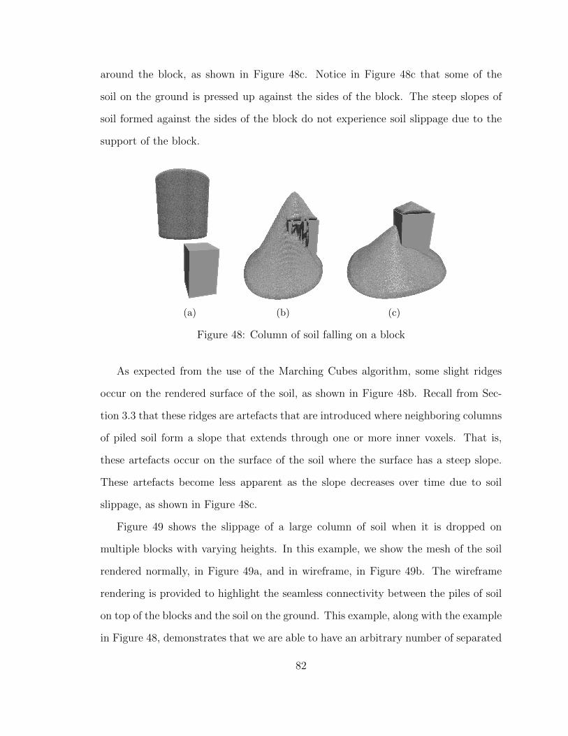
around the block, as shown in Figure 48c. Notice in Figure 48c that some of the
soil on the ground is pressed up against the sides of the block. The steep slopes of
soil formed against the sides of the block do not experience soil slippage due to the
support of the block.
(a) (b) (c)
Figure 48: Column of soil falling on a block
As expected from the use of the Marching Cubes algorithm, some slight ridges
occur on the rendered surface of the soil, as shown in Figure 48b. Recall from Sec-
tion 3.3 that these ridges are artefacts that are introduced where neighboring columns
of piled soil form a slope that extends through one or more inner voxels. That is,
these artefacts occur on the surface of the soil where the surface has a steep slope.
These artefacts become less apparent as the slope decreases over time due to soil
slippage, as shown in Figure 48c.
Figure 49 shows the slippage of a large column of soil when it is dropped on
multiple blocks with varying heights. In this example, we show the mesh of the soil
rendered normally, in Figure 49a, and in wireframe, in Figure 49b. The wireframe
rendering is provided to highlight the seamless connectivity between the piles of soil
on top of the blocks and the soil on the ground. This example, along with the example
in Figure 48, demonstrates that we are able to have an arbitrary number of separated
82

and connected soil piles at varying levels due to the use of a voxel grid. An effect such
as this has not been possible with previous heightfield and particle-based approaches
for real-time applications.
(a) Normal Rendering (b) Wireframe Rendering
Figure 49: Soil on multiple blocks
Shown in Figure 50 is a rigid block pushing a large quantity of soil across the
surface of a soil-filled landscape.
(a) (b)
(c) (d)
Figure 50: Soil pushed by a block
83

In this example, the moving block creates a path through the soil. The steep slopes on
the edges of this path experience soil slippage until the deformed soil behind the block
reaches a state of equilibrium. Figures 50a, 50b, and 50c show successive views of the
block pushing a mound of soil along the surface of the landscape. Figure 50d shows
the path that is created in the soil after the block has completely passed through it.
Shown in Figure 51 is a flat block digging and lifting a large quantity of soil out
of the ground. In this example, the block digs into the soil at an arbitrary location,
as shown in Figures 51a and 51b, slides under the soil, as shown in Figure 51c, and
scoops up a large quantity of soil, as shown in Figure 51d. Some of the soil that is
lifted out of the ground slips off the edges of the block and rejoins the soil on the
ground, as also shown in Figure 51d.
(a) (b)
(c) (d)
Figure 51: Soil lifted by a block
Because the static, loose, and falling soil in the simulation is represented in the
same voxel-based data structure, the rendered surface of the soil always maintains a
84

consistent appearance, regardless of the soil’s state.
The examples in Figures 50 and 51 show that our voxel-based soil simulation
system achieves goal 3 given in Section 1.1 (“Player-controlled objects should be ca-
pable of excavating and deforming the simulated soil in a manner that is as physically
realistic as done in previous approaches”). That is, the soil in our simulator can be de-
formed, displaced, excavated, and piled at arbitrary locations in the three-dimensional
environment.
4.1.3 Soil-Terrain Interaction
Figure 52 gives two screenshots that showcase the behavior of the simulated soil
when it is poured on a chunk of three-dimensional, voxel-based terrain. We achieve
this effect by constructing a collision field with a terrain density function [14], as
described in Section 2.2.2, as opposed to a set of rigid body volumes, as described
in Section 3.2.4. The terrain mesh is extracted from the collision field with the
Marching Cubes [27] and Transvoxel [23] algorithms, and rendered with a suitable,
rock-like texture.
(a) (b)
Figure 52: Soil on three-dimensional terrains
As shown in Figures 52a and 52b, the soil in our simulator can be piled on top of
complex, three-dimensional surfaces due to its voxel-based representation. Figure 52a
85

shows piles of soil at arbitrary locations on the landscape and Figure 52b shows a
portion of the simulated soil sliding down a steep, complex slope on the surface of a
voxel-based terrain.
4.2 Performance
We conducted a set of experiments to test the performance and scalability of our
voxel-based soil simulator. We performed these experiments on a computer with a
3.4GHz Intel Core i7-4770 CPU, 24GB of memory, a 2GB AMD Radeon R9 270 GPU,
and the Windows 8.1 operating system. As mentioned in Section 3.4.1, our simulator
is implemented using C++, DirectX 11, and HLSL. We use Visual Studio 2012 as the
integrated development environment for the simulator.
The performance of our simulator is affected by the resolution of the voxel grid that
is used to track the simulated soil. With a higher resolution voxel grid, the quality
of the simulation is increased, the surface of the simulated soil is more detailed, and
larger bodies of soil can be simulated. However, more operations are required at each
time step because there are more voxels to process. Therefore, the performance of the
simulation is decreased. Shown in Figure 53 is a clustered bar graph that visualizes
the maximum, average (mean), and minimum frame rates of our voxel-based soil
simulator when voxel grids with various resolutions are used. The resolutions used in
this experiment follow the format NxNxN , where N is the number of voxels along
each dimension of the grid. The frame rates for each resolution were recorded over 5
separate runs, where each run was a 30 second simulation of soil being pushed along
the surface by a rigid block. During this experiment, the simulator was configured to
perform 4 iterations of force propagation during each time step. The simulated soil
had the following properties: φ = 25, c = 0.0 t/m, and γ = 2.0 t/m2.
86

Figure 53: Frame rate versus resolution (1) (original in color)
The graph in Figure 53 shows that our simulator achieves goal 6 given in Sec-
tion 1.1 (“The system should operate in real-time with a minimum frame rate of
60 frames rendered per second”) when a voxel grid with a resolution of 56x56x56,
64x64x64, or 72x72x72 is used. The simulator operates close to, but slightly below,
60 frames per second when an 80x80x80 voxel grid is used. To achieve a minimum
frame rate of 60 frames per second with higher resolution voxel grids, a faster GPU
could be used or other parameters could be adjusted.
Shown in Figure 54 is a scatter plot that shows the average time, in milliseconds,
that our simulator took to render a frame of animation during the previous experi-
ment. This graph shows the relationship between milliseconds per frame, denoted by
t, and number of voxels, given by N3 and denoted by n. According to this graph, the
average time per frame increases linearly with the number of voxels. This linear rela-
tionship suggests that every voxel in the grid takes approximately the same amount
of time to process during a time step, regardless of the voxel grid’s resolution.
87

Figure 54: Time per frame versus number of voxels
By applying simple linear regression, we can determine the equation of the linear trend
line shown in Figure 54. That is, we can determine an equation that approximates
the average time needed to render a single frame of animation for a voxel grid with
any given number of voxels. This equation is given in Equation 36, where n is the
number of voxels in the grid and t is the average time per frame in milliseconds.
t = 2.4× 10⁻⁵n+ 4.3 where n ≥ 0 (36)
In this equation, the slope of the linear trend line is 2.4 × 10⁻⁵ ms/voxel and its y-
intercept is 4.3 ms. The slope is the average time, in milliseconds, that our simulator
takes to process a single voxel for a frame of animation. The y-intercept is the
average time per frame that our simulator takes to perform all other operations that
are separate from this algorithm. The y-intercept is also referred to as the overhead
of the simulation.
Shown in Figure 55 is a scatter plot that highlights the trend of the average frame
rate as the resolution was increased during the previous experiment.
88

Figure 55: Frame rate versus resolution (2)
Because the average frame rate is a reciprocal of t, given by 1000 ms/st
, and n = N3,
the equation of the trend line shown in Figure 55 can be derived from Equation 36,
as shown in Equation 37. That is, Equation 37 approximates the average frame rate
of the simulation, in frames per second, for any given value of N .
FPS =1000
2.4× 10⁻⁵N3 + 4.3where N ≥ 0 (37)
Shown in Figure 56 is a clustered bar graph that visualizes the maximum, average,
and minimum frame rates of our voxel-based soil simulator when various numbers of
force propagation iterations, denoted by α, are performed during each time step.
As in the previous experiment, the frame rates were recorded over 5 separate runs,
where each run was a 30 second simulation of soil being pushed along the surface by
a rigid block. During this experiment, a 72x72x72 voxel grid was used and all other
parameters were the same as for the previous experiment.
89
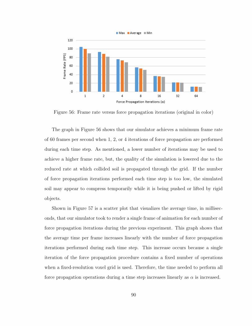
Figure 56: Frame rate versus force propagation iterations (original in color)
The graph in Figure 56 shows that our simulator achieves a minimum frame rate
of 60 frames per second when 1, 2, or 4 iterations of force propagation are performed
during each time step. As mentioned, a lower number of iterations may be used to
achieve a higher frame rate, but, the quality of the simulation is lowered due to the
reduced rate at which collided soil is propagated through the grid. If the number
of force propagation iterations performed each time step is too low, the simulated
soil may appear to compress temporarily while it is being pushed or lifted by rigid
objects.
Shown in Figure 57 is a scatter plot that visualizes the average time, in millisec-
onds, that our simulator took to render a single frame of animation for each number of
force propagation iterations during the previous experiment. This graph shows that
the average time per frame increases linearly with the number of force propagation
iterations performed during each time step. This increase occurs because a single
iteration of the force propagation procedure contains a fixed number of operations
when a fixed-resolution voxel grid is used. Therefore, the time needed to perform all
force propagation operations during a time step increases linearly as α is increased.
90

Figure 57: Time per frame versus force propagation iterations
By applying simple linear regression, we can determine the equation of the linear
trend line shown in Figure 57. That is, we can determine an equation that approx-
imates the average time needed to render a single frame of animation for any given
value of α. This equation is given in Equation 38, where α is the number of force
propagation iterations performed during each time step and t is the approximate time,
in milliseconds, per frame.
t = 1.17α + 8.95 where α ≥ 0 (38)
In this equation, the slope of the line is 1.17 ms/iteration and its y-intercept is
8.95 ms. The slope is the average time, in milliseconds, that our simulator takes to
perform a single iteration of the force propagation procedure when a 72x72x72 voxel
grid is used. The y-intercept is the average time per frame that our simulator takes to
perform all other operations. Equation 39 is used to calculate the average frame rate
of the simulation given the number of force propagation iterations performed during
each frame.
91

FPS =1000
1.17α + 8.95where α ≥ 0 (39)
By scaling the resolution of the voxel grid or adjusting the number of force prop-
agation iterations performed during a time step, the person running the simulation
should be able to find a desirable balance between quality and performance for a wide
variety of scenarios. Because of this flexibility, our simulator is suited to execution
on a wide variety of computers with low, medium, and high-end GPUs. Furthermore,
the linear relationships between the resolution and the time per frame and between
the number of iterations and the time per frame also show that our simulator achieves
goal 5 given in Section 1.1 (“The system should be robust and scalable, such that it
is capable of running efficiently on computers with various consumer level GPUs”).
Because our proposed voxel-based soil simulation system operates in real-time and
is robust and scalable, it is suited to be incorporated into computer games, video
games, simulation systems, and virtual reality systems.
4.3 Comparison
As discussed in Section 2.1.1, Sumner et al. and Li et al. developed models of
soil based on dynamically displaced heightmaps [26, 38]. The soil slippage model
proposed by Sumner et al. is a heuristic approach with empirically derived constants
[38]. The approach of Li et al. is physics-based and derives from the Mohr-Coulomb
failure criterion [9, 26]. The approach of Li et al. is more accurate than that of Sumner
et al. because it is capable of simulating the slippage of different types of soils based
on their internal friction, cohesion, and weight properties. Because our voxel-based
approach implements the soil slippage model proposed by Li et al., we achieve similar
results, as shown in Section 4.1.1. However, we use a multi-level heightfield, rather
92

than a two-dimensional heightfield, for soil slippage computations. Therefore, our
approach is capable of simulating the slippage of soil between an arbitrary number of
connected soil piles at various levels, as shown in Figures 48 and 49. The heightfield-
based approaches of Li et al. and Sumner et al. are capable of operating in real-time
[26, 38], as is our voxel-based approach, as shown in Section 4.2.
In addition to proposing a heuristic soil slippage model, Sumner et al. proposed
a method for simulating the compaction and subtle deformation of sand and soil-
filled landscapes [38]. In their approach, the soil on the ground is either compacted
downwards, based on a compaction ratio, or displaced horizontally when impacted
by a rigid body model or character. This compaction and displacement of soil results
in the creation of impressions, such as footprints and tire tracks, on the surfaces of
virtual landscapes. In our approach, tracks are created on the surface of the soil when
rigid objects push a quantity of soil along the surface, as shown in Figure 50. However,
we do not model the compaction of soils based on vertical impacts. Therefore, the
approach of Sumner et al. is more accurate than our approach when modeling subtle
deformations on the surfaces of sand and soil-filled landscapes.
Bell et al. and Zhu et al. proposed particle-based approaches that model bodies
of sand and soil as systems of rigid, spherical particles [3, 42]. Because the simulated
particles move independently and are not constrained by a two-dimensional grid,
the topology of the soil is able to evolve freely and form complex, three-dimensional
structures. As shown in Figures 48, 49, and 52, the simulated soils in our voxel-
based approach are also capable of forming complex, three-dimensional surfaces due
to the 3D nature of the voxel grid. However, the surface of the soil in our approach
is represented with a smooth, continuous mesh. In the particle-based approaches
of Bell et al. and Zhu et al., the surface of the soil is not continuous because each
spherical particle is rendered independently with a separate mesh. Furthermore, our
93

approach operates in real-time, as shown in Section 4.2, unlike the approaches of Bell
et al. and Zhu et al. [3, 42]. For example, while simulating an hourglass containing
approximately 100, 000 spherical particles, the approach of Bell et al. took an average
of 3.18 minutes to render each frame of animation [3]. While simulating the slippage
of a body of soil containing approximately 270, 000 particles, the approach of Zhu et
al. took approximately 6 seconds per frame [42].
Holz et al. proposed a hybrid approach that uses a two-dimensional heightfield to
represent the soil on the ground, in its generally static state, and a particle system to
represent loose soil, in its highly dynamic state [18]. In their approach, loose soils are
the soils on the ground surface that are being pushed, cut, or carved horizontally by
a rigid object. That is, the soil in their simulation is fixed on the ground surface and
cannot be excavated, lifted, or poured, as can be done in our voxel-based approach,
as shown in Figure 51. Furthermore, the soil in their simulation cannot be piled
on top of complex, three-dimensional surfaces due to the use of a two-dimensional
heightfield. The approach of Holz et al. significantly reduces the number of particles
required to achieve a realistic simulation because large scale features are modeled with
the efficient heightfield-based method, while small scale, highly dynamic features are
modeled with the better-suited particle-based approach. Like us, Holz et al. use the
soil slippage model proposed by Li et al. [26] to simulate the slippage of the soil
grid [18]. However, their approach models the compaction of soils based on vertical
impacts [18]. Therefore, their approach is capable of simulating subtle deformations,
such as footprints and tire tracks, on the surfaces of sand and soil-filled landscapes in a
manner similar to Sumner et al. [38]. As mentioned, we do not model the compaction
of soils in our voxel-based approach.
Onoue et al. proposed a hybrid approach that uses two-dimensional heightfields,
height span maps, and particle systems [32]. A two-dimensional heightfield is used to
94

model the soil on the ground, height span maps are used to model the soil piled on
top of objects, and a particle system is used to model falling quantities of soil. The
height span maps are used to represent the surfaces of soils piled on top of concave
objects with complex, three-dimensional surfaces. A height span map is similar to our
multi-level heightfield, but our multi-level heightfield represents the complete state
of the soil in the simulation, whereas a height span map, as used by Onoue et al.,
represents the surface of the soil resting on a single object [32]. Because the soil on
the ground, the soil piled on objects, and the falling soil are all represented in separate
data structures, Onoue et al. are not able to achieve seamless connectivity between
the soils on the ground and connecting soils on top of objects. However, we achieve
this seamless connectivity in our voxel-based approach, as shown in Figures 48 and
49, because the complete state of the soil is represented in a single data structure.
Furthermore, the soil slippage model used by Onoue et al. is based on the heuristic
approach of Sumner et al. [38]. Therefore, unlike our approach, it is not capable
of simulating the slippage of different types of soils based on their internal friction,
cohesion, and weight properties.
95
5 Conclusions and Future Work
In this chapter, we devote a section to each of the following: review, conclusions
and future work. In the first section, we provide a brief review of the body of this
thesis. In the second section, we present our conclusions and discuss the contributions
of our research. In the third section, we describe research that could be performed in
the future to continue the development of the work presented in this thesis.
5.1 Review
The research presented in this thesis is oriented towards the development of a
practical, real-time, graphical simulation of sands and soils. Simulating sands and
soils in a real-time computer graphics application is challenging due to the fine-grained
and highly dynamic nature of the materials. For example, footprints are left in the
sand after someone walks along a beach and mounds of soil can be dug out of the
ground and displaced in the environment with rigid tools and machinery. For this
research to achieve its desired level of realism in its simulation, the surfaces of sand
and soil-filled landscapes should react and deform naturally when excavation and
alteration activities are performed by the player at arbitrary locations. Furthermore,
steep slopes created on the surfaces of deformed soils should slip naturally based
on the type of soil being simulated. For the soil simulation system to be suited for
deployment in computer games, video games, simulations systems, and virtual reality
systems, it should operate in real-time with a minimum frame rate of 60 frames
rendered per second.
In our approach, a three-dimensional voxel grid is used to track the motion and
evolution of a quantity of soil in a three-dimensional space. The simulated soil in a
voxel grid is displaced over time based on three types of motion: projectile motion,
96

slippage motion, and contact motion. We adapted a voxel-based fluid advection
algorithm [16] to facilitate the displacement of falling soils based on projectile motion.
We adapted a heightfield-based soil slippage algorithm [26] to simulate the slippage
of soils in our voxel-based representation. We apply this soil slippage algorithm to
an indirect, multi-level heightfield representation of the soil instead of a voxel-based
representation. The voxel-based representation is updated afterwards to reflect the
changes made to the multi-level heightfield. The rigid bodies in the environment are
voxelized into the volumetric grid of the soil each frame to facilitate the detection
and resolution of per-voxel collisions between soil and rigid bodies. Our algorithms
for displacing soil in a voxel grid are designed to operate in parallel on current GPUs.
The soil is visualized each frame by extracting a surface mesh from the voxel grid with
a GPU-based implementation of the Marching Cubes [27] and Transvoxel algorithms
[23].
An empirical evaluation of our GPU-based implementation shows that our pro-
posed approach is capable of simulating complex, three-dimensional soil-object and
soil-terrain interactions, as well as the slippage of various types of sands and soils.
More specifically, this evaluation shows that, due to the use of a voxel grid, the soil
in our simulation can be piled on top of objects and terrains with complex, three-
dimensional surfaces. Furthermore, it is shown that the soil can be pushed, excavated,
lifted, and poured at arbitrary locations based on interactions with player-controlled
objects. It is also shown that our voxel-based approach is capable of representing
and simulating an arbitrary number of connected and separated soil piles at multiple
levels.
We conducted a set of experiments to test the performance and scalability of our
GPU-based implementation of the proposed algorithms. These experiments show
that our approach is capable of operating in real-time with a wide variety of voxel
97

grid resolutions. For example, it is shown that our simulator runs at approximately
74 frames per second when a grid containing 373, 248 voxels is used. It is also shown
that our simulator runs at approximately 58 frames per second, which is slightly
below our goal of 60 frames per second, when a voxel grid containing 512, 000 voxels
is used. When a voxel grid containing over one million voxels is used, our simulator
runs at approximately 31 frames per second. In these experiments, it is shown that
the average time our simulator takes to render a single frame of animation increases
linearly with the number of voxels in the voxel grid. Similarly, the average time per
frame increases linearly with the number of force propagation iterations performed
during each time step.
Because the soil slippage algorithm used in our approach is based on the algorithm
proposed by Li et al. [26], we achieve similar results, including being able to simulate
the slippage of various types of soils based on their internal friction, cohesion, and
weight properties. This soil slippage algorithm is an improvement over the heuristic
approaches of Sumner et al. [38] and Onoue et al. [32] because it models the underlying
physics of soil movement. However, Sumner et al. and Holz et al. proposed methods
for simulating soil compaction [18, 38], which is a behavior of soil that we do not
model in our approach. Due to the three-dimensional nature of a voxel grid, our
approach is able to simulate bodies of soils with complex, three-dimensional surfaces,
similar to previous particle-based approaches [3, 42]. However, these particle-based
approaches are not suited for simulating large bodies of soil in real-time. Furthermore,
the surfaces of particle-based soils are not continuous because each particle is rendered
independently with a separate mesh. The multi-level heightfield used in our approach
is similar to the height span maps used by Onoue et al. [32], but our multi-level
heightfield represents the complete state of the soil. Because of this representation,
we are able to simulate the slippage of soil along slopes that connect soil on the ground
98

to soil above objects.
5.2 Conclusions
This thesis provides a novel, voxel-based approach to simulating sands and soils
on the GPU in real-time computer graphics applications. This soil simulation system
is practical, robust, and scalable. Therefore, it suited for incorporation into computer
games, video games, simulation systems, and virtual reality systems. To our knowl-
edge, a complete, voxel-based approach to simulating sands and soils has not been
presented previously in literature.
Due to the three-dimensional nature of a voxel grid, our approach is capable
of simulating various effects that are not possible in previous real-time approaches.
These effects include the following:
• Sands and soils piled on the surface of complex, three-dimensional, voxel-based
terrains.
• Smooth, seamless surfaces between soil piled on the ground and soil piled on
top of objects.
• Arbitrary numbers of connected and separated soil piles at various levels.
• Consistent, mesh-based appearance of piled, loose, and falling soils.
However, our proposed approach does not simulate all characteristics and behaviors
of soils that are modeled in previous approaches. For example, we do not model the
compaction of soils based on impacts with rigid bodies. Furthermore, soils piled on a
moving object do not move uniformly with the object because we do not consider the
frictional forces between contacting bodies of soil and rigid objects. This limitation
is discussed in more detail in Section 5.3.1. Because there are characteristics and
99

behaviors of soils that we do not model in our approach, the research presented
in this thesis leaves future research opportunities that may lead to more realistic
simulations.
Overall, we have made the following contributions by the research presented in
this thesis:
• We introduced a novel, voxel-based representation of sands and soils that rep-
resents a quantity of soil in a three-dimensional grid.
• We presented a voxel volume constraint, and novel methods for satisfying this
constraint during a GPU-based simulation.
• We adapted a fluid advection algorithm to facilitate the displacement of soil
density in a voxel grid in parallel.
• We provided a set of algorithms for resolving density overflows in a voxel grid
on the GPU.
• We adapted a heightfield-based soil slippage algorithm to operate in parallel on
piles of soil at multiple levels in a voxel grid.
• We introduced a novel, parallel algorithm for propagating quantities of soil
through a voxel grid based on collisions with rigid objects and bodies.
• We presented the first GPU-based implementation of the proposed algorithms.
• We presented the first empirical evaluation of the parallel approach implemented
on the GPU.
In Section 1.1, we listed a set of goals for the research presented in this thesis. For
convenience, these goals are listed again:
100

1. A dynamic terrain rendering system should be developed that produces realis-
tic renderings and simulations of sand and soil-filled landscapes in a real-time
computer graphics application.
2. The system should be capable of simulating several types of soils with varying
cohesion, friction, and weight properties.
3. Player-controlled objects should be capable of excavating and deforming the
simulated soil in a manner that is as physically realistic as done in previous
approaches.
4. Unstable slopes on the surfaces of soils should cause the soil to slide in a phys-
ically accurate manner based on the type of soil that is being simulated.
5. The system should be robust and scalable, such that it is capable of running
efficiently on computers with various consumer level GPUs.
6. The system should operate in real-time with a minimum frame rate of 60 frames
rendered per second.
As demonstrated in Chapter 4, all of these goals were achieved.
5.3 Future Work
In this section, we describe potential research that could be performed to further
the development of the ideas presented in this thesis. We devote a subsection to
each potential research opportunity: soil on moving objects, removal of ridge arte-
facts, compaction and consolidation, and moisture content. In the first subsection,
we discuss possible ways of overcoming a limitation of our approach related to the
displacement of soil resting above moving objects. In the second subsection, we de-
scribe a potential approach to removing the vertical ridge artefacts that appear on
101

the surfaces of soils with steep slopes. In the third subsection, we discuss the com-
paction and consolidation of soils, which is a behavior of soil that we do not model
in our proposed approach. Lastly, in the fourth subsection, we briefly discuss the
relationship between a quantity of soil’s moisture content and its shear strength. We
also describe a potential method for simulating bodies of soil with varying moisture
contents.
5.3.1 Soil on Moving Objects
To extend this research to allow the handling of soil piled on moving objects, a
method could be devised to facilitate the horizontal displacement of soils resting on
rigid objects or bodies. In our approach, the soil above an object slides frictionlessly
off the edges of the object when the object has a horizontal motion, as shown in
Figure 58.
(a) (b)
(c) (d)
Figure 58: Soil sliding off a frictionless block
102

The soil slips off the edges of the object because we do not model the frictional forces
that occur between contacting bodies of soil and rigid objects. Figure 58a shows a
pile of soil resting above a rigid object. The soil above this object was lifted out of the
ground beneath the object, leaving a moderately sized hole. Figures 58b, 58c, and 58d
show successive views of the rigid object moving horizontally away from the player’s
viewpoint. Figures 58b and 58c show the soil above the object sliding and falling
off the edge of the object as the object moves away from the viewpoint. Figure 58d
shows the soil rejoined with the ground, such that the hole shown in Figure 58a is
refilled.
In previous approaches, a separate data structure is used to represent the soil
piled on top of each object in the simulation. That is, the soil on an object is
represented in the local space of that object. Therefore, as the object moves, the soil
in its respective data structure moves with it. However, because our approach uses
a single, voxel-based data structure to represent the complete state of the soil, an
alternative method should be developed to facilitate the horizontal displacement of
soils resting on moving, rigid objects.
5.3.2 Removal of Ridge Artefacts
In our approach, slight, regularly spaced, vertical ridges occur on the surfaces of
soils that have steep slopes, as discussed in Section 3.3. These ridges cause shading
artefacts to appear on the surfaces of soils, thereby reducing the visual quality and
naturalness of the simulation. Continuing the development of this research, a method
could be devised to hide or eliminate these vertical ridges. One possible approach to
eliminating these vertical ridges is to modify the values in the density field, before
the mesh extraction process, such that the Marching Cubes algorithm produces a
desirable surface with no ridges. A two-dimensional example of this modification is
103
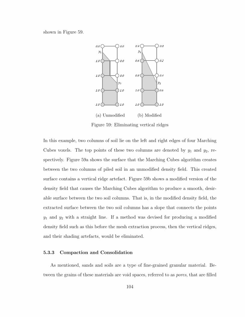
shown in Figure 59.
(a) Unmodified (b) Modified
Figure 59: Eliminating vertical ridges
In this example, two columns of soil lie on the left and right edges of four Marching
Cubes voxels. The top points of these two columns are denoted by y1 and y2, re-
spectively. Figure 59a shows the surface that the Marching Cubes algorithm creates
between the two columns of piled soil in an unmodified density field. This created
surface contains a vertical ridge artefact. Figure 59b shows a modified version of the
density field that causes the Marching Cubes algorithm to produce a smooth, desir-
able surface between the two soil columns. That is, in the modified density field, the
extracted surface between the two soil columns has a slope that connects the points
y1 and y2 with a straight line. If a method was devised for producing a modified
density field such as this before the mesh extraction process, then the vertical ridges,
and their shading artefacts, would be eliminated.
5.3.3 Compaction and Consolidation
As mentioned, sands and soils are a type of fine-grained granular material. Be-
tween the grains of these materials are void spaces, referred to as pores, that are filled
104

with quantities of air and water [6]. When a sand or soil-filled landscape is struck by
a rigid object or body, the air and water in these pores are released and the soil is
compacted and consolidated. As mentioned in Section 4.3, Sumner et al. and Holz
et al. proposed heightfield-based methods for simulating the compaction of sand and
soil-filled landscapes [38, 18]. In their approaches, impressions, such as footprints and
tire tracks, are created on the surfaces of virtual landscapes as a result of impacts
caused by rigid objects and characters. In our approach, we do not model the com-
paction of sands and soils based on these types of impacts. In the future, a method
could be devised to facilitate the compaction and consolidation of the soils in our
proposed voxel-based simulation. This method might be adapted from the methods
of Sumner et al. [38] and Holz et al. [18], or it might be a novel approach.
5.3.4 Moisture Content
The shear strength of a body of soil is affected by its moisture content, which is
the amount of water contained in the pores of its material [6, 9]. For example, grains
of sand have a greater tendency to stick together and interlock when they are wet.
Therefore, wet sands are less prone to soil slippage and have a higher angle of repose
than dry sands. To enhance the approach described in this thesis, a method could be
devised to simulate bodies of voxel-based soil with varying moisture contents. One
possible approach is to use a 3D property field, similar to the density, velocity, and
force fields, to record the moisture content of the soil in each voxel of the grid. Based
on values in this field, the coefficient of cohesion associated with the soil in a voxel
could be altered to account for the increase or decrease in shear strength. Also, the
surface of the soil could be darkened and increased in specularity in proportion to the
moisture content, such that the rendered surface appears to be wet when the moisture
content is high.
105

References
[1] Aquilio, A. S., Brooks, J. C., Zhu, Y., and Owen, G. S. Real-time GPU-
based simulation of dynamic terrain. In Proceedings of the Second International
Conference on Advances in Visual Computing (2006), Springer, pp. 891–900.
[2] Balovnev, V. I. New Methods for Calculating Resistance to Cutting of Soil.
Translated from Russian, Published for the U.S. Department of Agriculture and
the National Science Foundation, Washington, D.C., 1983.
[3] Bell, N., Yu, Y., and Mucha, P. J. Particle-based simulation of granular
materials. In Proceedings of the 2005 ACM SIGGRAPH/Eurographics Sympo-
sium on Computer Animation (2005), ACM, pp. 77–86.
[4] Brackbill, J., and Ruppel, H. FLIP: a method for adaptively zoned,
particle-in-cell calculations of fluid flows in two dimensions. Journal of Com-
putational Physics 65 (1986), 314–343.
[5] Bridson, R., and Muller-Fischer, M. Fluid Simulation: SIGGRAPH 2007
Course Notes. ACM, 2007.
[6] Bromhead, E. The Stability of Slopes. Surrey University Press, 1986.
[7] Cat Simulators. Hydraulic excavator training simulator. http://www.
catsimulators.com. Accessed: 2015-03-11.
[8] Chentanez, N., and Muller, M. Real-time simulation of large bod-
ies of water with small scale details. In Proceedings of the 2010 ACM SIG-
GRAPH/Eurographics Symposium on Computer Animation (2010), Eurograph-
ics Association, pp. 197–206.
106
[9] Chowdhury, R. Slope Analysis. Elsevier North-Holland Inc., 1978.
[10] Cohen-Or, D., and Kaufman, A. Fundamentals of surface voxelization.
Graphical Models and Image Processing 57 (1995), 453–461.
[11] De Boer, W. H. Fast terrain rendering using geometrical mipmapping. Unpub-
lished paper, available at http://www. flipcode. com/articles/article geomipmaps
(2000).
[12] Dong, Z., Chen, W., Bao, H., Zhang, H., and Peng, Q. Real-time
voxelization for complex polygonal models. In Proceedings of the 12th Pacific
Conference on Computer Graphics and Applications (2004), IEEE, pp. 43–50.
[13] Drebin, R. A., Carpenter, L., and Hanrahan, P. Volume rendering. In
Proceedings of the 15th Annual Conference on Computer Graphics and Interac-
tive Techniques (1988), ACM, pp. 65–74.
[14] Geiss, R. Generating complex procedural terrains using the GPU. GPU Gems
3 (2007), 7–37.
[15] Giancoli, D. Physics: Principles with Applications, Sixth ed. Addison-Wesley,
2004.
[16] Hamilton, H. Animation Software Design: Course Notes. Department of
Computer Science, University of Regina, 2015.
[17] Harlow, F. H. The particle-in-cell method for numerical solution of problems
in fluid dynamics. In Experimental Arithmetic, High-Speed Computations and
Mathematics (1963).
107
[18] Holz, D., Beer, T., and Kuhlen, T. Soil deformation models for real-time
simulation: a hybrid approach. In Workshop in Virtual Reality Interactions and
Physical Simulation (2009), Eurographics Association, pp. 21–30.
[19] Ikits, M., Kniss, J., Lefohn, A., and Hansen, C. Volume rendering
techniques. GPU Gems 1 (2004).
[20] Jensen, L. S., and Golias, R. Deep-water animation and rendering. In Game
Developers Conference (Gamasutra) (2001).
[21] John Deere. Excavator training simulator. https://www.deere.com/en_
ASIA/services_and_support/product_training/construction_operator_
training/level_2_simulator/level_2_simulator.page. Accessed: 2015-03-
11.
[22] Laprairie, M. ICVG: Practical Constructive Volume Geometry for Indirect
Visualization. Master’s thesis, Department of Computer Science, University of
Regina, 2011.
[23] Lengyel, E. S. Voxel-Based Terrain for Real-Time Virtual Simulations. PhD
thesis, University of California at Davis, 2010.
[24] LevelDev. Heightmap. https://leveldev.wordpress.com/2012/12/04/
landscapesparti/heightmap. Accessed: 2015-03-11.
[25] Levoy, M. Display of surfaces from volume data. IEEE Computer Graphics
and Applications 8, 3 (1988), 29–37.
[26] Li, X., and Moshell, J. M. Modeling soil: realtime dynamic models for soil
slippage and manipulation. In Proceedings of the 20th Annual Conference on
Computer Graphics and Interactive Techniques (1993), ACM, pp. 361–368.
108

[27] Lorensen, W. E., and Cline, H. E. Marching cubes: a high resolution 3D
surface construction algorithm. In Proceedings of the 14th Annual Conference
on Computer Graphics and Interactive Techniques (1987), ACM, pp. 163–169.
[28] Losasso, F., and Hoppe, H. Geometry clipmaps: terrain rendering using
nested regular grids. In ACM Transactions on Graphics (2004), vol. 23, ACM,
pp. 769–776.
[29] Ludin, J. Heavy equipment simulators provide a risk-free training
solution. http://nccercornerstone.org/industry/tech-talk/item/
129-heavy-equipment-simulators-provide-a-risk-free-training-solution,
2013. Accessed: 2015-03-11.
[30] Michael, D. R., and Chen, S. L. Serious Games: Games that Educate,
Train, and Inform. Thomson Course Technology, 2006.
[31] Morgan, R. P. C. Soil Erosion and Conservation, Third ed. Wiley-Blackwell,
2005.
[32] Onoue, K., and Nishita, T. Virtual sandbox. In Proceedings of the 11th Pa-
cific Conference on Computer Graphics and Applications (2003), IEEE, pp. 252–
259.
[33] Parent, R. Computer Animation: Algorithms and Techniques, Third ed. Mor-
gan Kaufmann, 2012.
[34] Peck, R. B., Hanson, W. E., and Thornburn, T. H. Foundation Engi-
neering, Second ed. Wiley, 1974.
[35] Prensky, M. Computer games and learning: digital game-based learning.
Handbook of Computer Game Studies 18 (2005), 97–122.
109

[36] Stam, J. Stable fluids. In Proceedings of the 26th Annual Conference on
Computer Graphics and Interactive Techniques (1999), ACM/Addison-Wesley,
pp. 121–128.
[37] Strugar, F. Continuous distance-dependent level of detail for rendering
heightmaps. Journal of Graphics, GPU, and Game Tools 14 (2009), 57–74.
[38] Sumner, R. W., O’Brien, J. F., and Hodgins, J. K. Animating sand,
mud, and snow. In Computer Graphics Forum (1999), vol. 18, Wiley Online
Library, pp. 17–26.
[39] Tessendorf, J. Simulating Ocean Water: SIGGRAPH 2001 Course Notes.
ACM, 2001.
[40] Virtual Terrain Project. Global elevation datasets. http://vterrain.
org/Elevation/global.html. Accessed: 2015-03-11.
[41] Wang, D., and Wang, C. Real-time GPU-based simulation of dynamic terrain
in virtual battlefield. Journal of Computational Information Systems 7, 6 (2011),
1924–1933.
[42] Zhu, Y., and Bridson, R. Animating sand as a fluid. ACM Transactions on
Graphics 24, 3 (2005), 965–972.
110