a wavelet interpolation galerkin method for the...

Hindawi Publishing CorporationMathematical Problems in EngineeringVolume 2010, Article ID 586718, 25 pagesdoi:10.1155/2010/586718

Research ArticleA Wavelet Interpolation Galerkin Method forthe Simulation of MEMS Devices under the Effectof Squeeze Film Damping

Pu Li1 and Yuming Fang2

1 School of Mechanical Engineering, Southeast University, Jiangning, Nanjing 211189, China2 College of Electronic Science and Engineering, Nanjing University of Posts and Telecommunications,Nanjing 210003, China

Correspondence should be addressed to Pu Li, [email protected]

Received 29 March 2009; Revised 17 September 2009; Accepted 27 October 2009

Academic Editor: Stefano Lenci

Copyright q 2010 P. Li and Y. Fang. This is an open access article distributed under the CreativeCommons Attribution License, which permits unrestricted use, distribution, and reproduction inany medium, provided the original work is properly cited.

This paper presents a new wavelet interpolation Galerkin method for the numerical simulationof MEMS devices under the effect of squeeze film damping. Both trial and weight functions area class of interpolating functions generated by autocorrelation of the usual compactly supportedDaubechies scaling functions. To the best of our knowledge, this is the first time that wavelets havebeen used as basis functions for solving the PDEs of MEMS devices. As opposed to the previouswavelet-based methods that are all limited in one energy domain, the MEMS devices in the paperinvolve two coupled energy domains. Two typical electrically actuated micro devices with squeezefilm damping effect are examined respectively to illustrate the new wavelet interpolation Galerkinmethod. Simulation results show that the results of the wavelet interpolation Galerkin methodmatch the experimental data better than that of the finite difference method by about 10%.

1. Introduction

Modeling and simulation of MEMS devices play an important role in the design phase forsystem optimization and for the reduction of design cycles. The performances of MEMSdevices are represented by partial-differential equations (PDEs) and associated boundaryconditions. In the past two decades, there have been extensive, and successful, works focusedon solving the partial-differential equations of MEMS [1–15]. A detailed review of the worksis available in [1]. In the previous works, Galerkin method was widely used to reduce thepartial-differential equations to ordinary-differential equations (ODEs) in time and then solvethe reduced equations either numerically or analytically. The previous works differ from eachother in the choice of the basis functions.

2 Mathematical Problems in Engineering

The basis set can be chosen arbitrarily, as long as its elements satisfy all of the boundaryconditions and are sufficiently differentiable. To enhance convergence, the basis set has tobe chosen to resemble the behavior of the device. For example, two ways have been usedto generate the basis set for the reduced-order models of MEMS devices [1]. The first way[4, 9] uses the undamped linear model shapes of the undeflected microstructure as basisfunctions. For simple structures with simple boundary conditions, the mode shapes are foundanalytically. For complex structures or complex boundary conditions, the linear mode shapesare obtained numerically using the finite element method. The second way [2] conductsexperiments or solves the PDEs using FEM or FDM to generate snapshots under a trainingsignal, then applies a modal analysis method (one of the variation of the proper orthogonaldecomposition method [6]) to the time series to extract the mode shapes of the devicestructural elements.

In the past two decades also, a new numerical concept was introduced and is gainingincreasing popularity [16–25]. The method is based on the expansion of functions in terms ofa set of basis functions called wavelets. Indeed wavelets have many excellent properties suchas orthogonality, compact support, exact representation of polynomials to a certain degree,and flexibility to represent functions at different levels of resolution. Indeed a completebasis can be generated easily by a signal function through dilatation and translation. Thewavelet-based methods may be classified as wavelet-Galerkin method [19, 20], wavelet-collocation method [21, 22], and wavelet interpolation Galerkin method [23–25]. Amongthe three methods, the wavelet-Galerkin method is the most common one because of itsimplementation simplicity. The method is a Galerkin scheme using scaling or waveletfunctions as the trial and weight functions. However, both scaling and wavelet functionsdo not satisfy the boundary conditions. Thus the treatment of general boundary conditionsis a major difficulty for the application of the wavelet-Galerkin method, especially for thebounded region problems, even though different efforts [19, 20] have been made. For thewavelet-collocation method, boundary conditions can be treated in a satisfactory way [21]. Inthe method, trial functions are a class of interpolating functions generated by autocorrelationof the usual compactly supported Daubechies scaling functions. However, the methodrequires the calculation of higher-order derivatives (up to the second derivatives for second-order parabolic problems) of the wavelets. Due to the derivatives of compactly supportedwavelets being highly oscillatory, it is difficult to compute the connection coefficients bythe numerical evaluation of integral [18]. The wavelet interpolation Galerkin method is aGalerkin scheme that both trial and weight functions are a class of interpolating functionsgenerated by autocorrelation of the usual compactly supported Daubechies scaling functions.For the method, the boundary conditions [24] can be treated easily and the formulations arederived from the weak form; thus only the first derivatives of wavelets (for second-orderparabolic problems) are required.

Wavelets have proven to be an efficient tool of analysis in many fields including thesolution of PDEs. However, few papers in MEMS area give attention to the wavelet-basedmethods. This paper presents a new wavelet interpolation Galerkin method for the numericalsimulation of MEMS devices under the effect of squeeze film damping. To the best of ourknowledge, this is the first time that wavelets have been used as basis functions for solvingthe PDEs of MEMS devices. As opposed to the previous wavelet-based methods that are alllimited in one energy domain, the MEMS devices in the paper involve two coupled energydomains. The squeeze film damping effect on the dynamics of microstructures has alreadybeen extensively studied. We stress that our intention here is not to discover new physics tothe squeeze film damping.

Mathematical Problems in Engineering 3

The outline of this paper is as follows. Section 2 presents a brief introduction to somemajor concepts and properties of wavelets. In Sections 3 and 4, two typical electricallyactuated micro devices with squeeze film damping effect are examined respectively toillustrate the wavelet interpolation Galerkin method. Section 5 calculates the frequencyresponses and the quality factors using the present method, and compares the calculatedresults with those generated by experiment [26, 27], by the finite difference method, and byother published analytical models [15, 26]. Finally, a conclusion is given in Section 6.

2. Basic Concepts of Daubechies’ Wavelets and Wavelet Interpolation

In this section, we shall give a brief introduction to the concepts and properties of Daubechies’wavelets. More detailed discussions can be found in [16–18, 21].

2.1. Daubechies’ Orthonormal Wavelets

Daubechies [16, 17] constructed a family of orthonomal bases of compactly supportedwavelets for the space of square-integrable funcntions, L2(R). Due to the fact that they possessseveral useful properties, such as orthogonality, compact support, exact representation ofpolynomials to a certain degree, and ability to represent functions at different levels ofresolution, Daubechies’ wavelets have gained great interest in the numerical solutions ofPDEs [18–22].

Daubechies’ functions are easy to construct [16, 17]. For an even integer L, we havethe Daubechies’ scaling function φ(x) and wavelet ψ(x) satisfying

φ(x) =L−1∑

i=0

piφ(2x − i)

ψ(x) =1∑

i=2−L(−1)ip1−iφ(2x − i).

(2.1)

The fundamental support of the scaling function φ(x) is in the interval [0, L − 1] while thatof the corresponding wavelet ψ(x) is in the interval [1 − L/2, L/2]. The parameter L will bereferred to as the degree of the scaling function φ(x). The coefficients pi are called the waveletfilter coefficients. Daubenchies [16, 17] established these wavelet filter coefficients to satisfythe following conditions:

L−1∑

i=0

pi = 2,

L−1∑

i=0

pipi−m = δ0,m,

1∑

i=2−L(−1)ip1−ipi−2m = 0 for integer,

L−1∑

i=0(−1)iimpi = 0, m = 0, 1, . . . ,

L

2− 1,

(2.2)


where δ0,m is the Kronecker delta function. Correspondingly, the constructed scanlingfunction φ(x) and wavelet ψ(x) have the following properties:

∫∞

−∞φ(x)dx = 1,

∫∞

−∞φ(x − i)φ(x −m)dx = δi,m for integers i,m,

∫∞

−∞φ(x)ψ(x −m)dx = 0 for integer m,

∫∞

−∞xmψ(x)dx = 0, m = 0, 1, . . . ,

L

2− 1.

(2.3)

Denote by L2(R) the space of square-integrable functions on the real line. Let VJ andWJ be the subspace generated, respectively, as the L2-closure of the linear spans of φJ,i(x) =2J/2φ(2Jx − i) and ψJ,i(x) = 2J/2ψ(2Jx − i), J, i ∈ Z. Z denotes the set of integers. Then (2.3)implies that

VJ+1 = VJ ⊕WJ, V0 ⊂ V1 ⊂ · · ·VJ ⊂ VJ+1, VJ+1 = V0 ⊕W0 ⊕W1 ⊕ · · ·WJ, (2.4)

Equation (2.4) presents the multiresolution properties of wavlets. Any function f ∈ L2(R),may be approximated by the multiresolution apparatus described above, by its projectionPVJ f onto the subspaceVJ

PVJ f =∑

i∈ZfJ,iφJ,i(x). (2.5)

2.2. Wavelet Interpolation Scaling Function

For a given Daubechies’ scaling function, its autocorrelation function θ(x) can be defined asfollows [21]:

θ(x) =∫∞

−∞φ(τ)φ(τ − x)dτ. (2.6)

The function satisfies the following interpolating property

θ(k) = δ0,k, k ∈ Z, (2.7)

and has a symmetric support [−(L − 1), (L − 1)]. The derivative of the function θ(k) may becomputed by differentiating the convolution product

θ(s)(k) = (−1)(s)∫∞

−∞φ(τ)φ(s)(τ − k)dτ. (2.8)


Let θ(x) act as the scaling function, we have

θJ,k(x) = θ(

2Jx − k), k ∈ Z. (2.9)

For a set of dyadic grids of the type xJk ∈ R: xJk = 2−Jk, where k, J ∈ Z, the θJ,k(x) verifies theinterpolation property at the dyadic points: θJ,k(x

Jn) = δn,k. Let V x

J be the linear span of theset {θ(2Jx − k), k ∈ Z}. It can be proved that {V x

J } forms a multiresolution analysis, whereθJ,k(x) acts as the role of scaling function (the so-called interpolation scaling function), andthe set {θ(2Jx−k), k ∈ Z} is a Riesz’s basis for V x

J . For a function f ∈ H1(R), an interpolationoperator IJ : H1(R) → V x

J can be defined [21]:

IJ(f)=∑

k

fJkθ(

2Jx − k), k ∈ Z, (2.10)

where fJk = f(xJk) = f(2−Jk). Thus, for a function f(x) defined on x ∈ [0, 1], f(x) has thefollowing approximation

f(x) =2J+(L−1)∑

k=−(L−1)

fJ,kθ(

2Jx − k)

=1∑

k=−(L−1)

fJ,kθ(

2Jx − k)+

2J∑

k=0

fJ,kθ(

2Jx − k)+

2J+L−1∑

k=2J+1

fJ,kθ(

2Jx − k).

(2.11)

In this paper, wavelet collocation scheme is applied on x ∈ [0, 1], where xJk = 2−Jkand k = 0, 1, . . . , 2J . Therefore, instead of the values of f(x) at xJ

k, k = −(L − 1), . . . ,−1 and

k = 2J + 1, . . . , (L − 1), we may use some values which are extrapolated from the values inthose dyadic points internal to the interval x ∈ [0, 1]. As described in [21, 22], we define

f(x) =2J∑

k=0

fJ,kθ(

2Jx − k), (2.12)

where

θ(

2Jx − k)=

⎧⎪⎪⎪⎪⎪⎪⎪⎪⎪⎨

⎪⎪⎪⎪⎪⎪⎪⎪⎪⎩

θ(2Jx − k

)+

−1∑

n=−(L−1)

ankθ(2Jx − n

), k = 0, 1, . . . , 2M − 1

θ(2Jx − k

), k = 2M, . . . , 2J − 2M

θ(2Jx − k

)+

2J+L−1∑

n=2J+1

bnkθ(2Jx − n

), k = 2J − 2M + 1, . . . , 2J ,

(2.13)


where the coefficients ank and bnk are defined by

ank = l1k(xJn

), bnk = l2k

(xJn

), (2.14)

where l1k(x) and l2k(x) represent Lagrange interpolation polynomials, defined by

l1k(x) =2M−1∏

i=0i /= k

x − xJixJk− xJi

, l2k(x) =2J∏

i=2J−2M+1i /= k

x − xJixJk− xJi

. (2.15)

An analogous manner can be given for two-dimensional problem. By using tensorproducts, it is then possible to define a multiresolution on the square x, y ∈ [0, 1]. The two-dimensional scaling function is defined by ΘJ

k,k′(x, y) =

∑2Jk=0∑2J

k′=0 fJk,k′θ(2Jx − k)θ(2Jy − k′).

Let V xy

J = V xJ ⊗V

y

J be the linear span of the set {θ(2Jx−k)θ(2Jy−k′), J, k, k′ ∈ Z}; thus the set{V xy

J } forms a multiresolution analysis and the set {θ(2Jx − k)θ(2Jy − k′), k, k′ ∈ Z} is a Rieszbasis for {V xy

J }. Therefore, for a function f(x, y) defined on x, y ∈ [0, 1], it has the followingapproximation:

f(x, y)=

2J∑

k=0

2J∑

k′=0

fJk,k′θ(

2Jx − k)θ(

2Jy − k′). (2.16)

3. Wavelet Interpolation Galerkin Method fora Parallel Plate Microresonator under the Effect ofSqueeze Film Damping

3.1. Governing Equations

In this section, we examine the example of a rectangular parallel plate under the effect ofsqueeze film damping. As shown in Figure 1, the rectangular parallel plate is excited bya conventional voltage. The voltage is composed of a dc component V0 and a small accomponent v(t), V0 v(t). The plate is rigid. The displacement of the plate under the electricforce is composed of a static component to the dc voltage, denoted by z0, and a small dynamiccomponent due to the ac voltage, denoted by z(t), z0 z(t), that is,

zE(t) = z0 + z(t). (3.1)

The equation of motion that governs the displacement of the plate is written as

mplatezE + kspringzE =εAplate(V0 + v)2

2(g0 − zE

)2− f(t), (3.2)

where mplate is the mass of the plate, Aplate is the are of the plate, kspring is the stiffness of thespring, g0 is the zero-voltage air gap spacing, ε is the dielectric constant of the gap medium,


k

x

z

V0 + ν(t)

(a) Side view of the microplate

x

z

(b) Top view of the microplate

Figure 1: A schematic drawing of an electrically actuated microplate under the effect of squeeze filmdamping.

f(t) is the force acting on the plate owing to the pressure of the squeeze gas film between theplate and the substrate.

We expand (3.2) in a Taylor series around V0 and z0 up to first order and rewrite (3.2)as

mplatez + kEz =εAplateV0

g20

v − f(t), (3.3)

where kE = kspring − (εAplateV20 /(g0 − z0

)3), g0 = g0 − z0. The force f(t) acting on the plateowing to the pressure of the squeeze gas film is given by

f(t) =∫ ly

0

∫ lx

0

(p(x, y, t

)− p0)dxdy, (3.4)

where lx and ly are the length and width of plate, p(x, y, t) is the absolute pressure in the gapand p0 is the ambient pressure. The pressure p(x, y, t) is governed by the nonlinear Reynoldsequation [3]

∂

∂x

(h3p

∂p

∂x

)+

∂

∂y

(h3p

∂p

∂y

)= 12ηeff

(h∂p

∂t+ p

∂h

∂t

), (3.5)

where h(x, t) = g0 − z0 − z(t) = g0 − z(t) and ηeff is the effective viscosity of the fluid in thegap. In this section, all edges of the rectangular plate are ideally vented; thus the pressureboundary conditions for the case in Figure 1 are

p(x, 0, t) = p(x, ly, t

)= p(0, y, t

)= p(lx, y, t

)= p0. (3.6)

For convenience, we introduce the nondimensional variables

X =x

lx, Y =

y

ly, Z =

z

g0, P =

p

p0, T =

t

S, H =

h

g0= 1 − Z, (3.7)


where T is a timescale, S =√mplate/kE = 1/ωn, ωn is the nature frequency of the plate.

Substituting (3.7) into (3.3)–(3.6), we obtain

d2Z

dT2+ Z = αV0v − Pnon

∫∫1

0

(P − 1

)dX dY, (3.8)

∂

∂X

(H3P

∂P

∂X

)+ β2 ∂

∂Y

(H3P

∂P

∂Y

)=σ

S

(H∂P

∂T+ P

∂H

∂T

), (3.9)

where α = εAplate/kEg30 , Pnon = p0lxly/kEg0, σ = 12ηeffl

2x/g

20p0, and β = lx/ly. The

nondimensional boundary conditions are

P(X, 0, T) = P(X, 1, T) = P(1, Y, T) = P(0, Y, T) = 1. (3.10)

As mentioned above, the microplate is under small oscillation around g0 and thereforethe pressure variation from ambient in the squeeze film is also small, P(X,Y, T) is given by

P(X,Y, T) =p

p0= 1 + P(X,Y, T), (3.11)

where |P(X,Y, T)| 1. Substituting (3.11) into (3.9), and linearizing the outcome around p0

and g0, we obtain

∂2P

∂X2+ β2 ∂

2P

∂Y 2− σS

∂P

∂T= −σ

S

∂Z

∂T. (3.12)

The boundary conditions for the case are

P(X, 0, T) = P(X, 1, T) = P(0, Y, T) = P(1, Y, T) = 0. (3.13)

For a harmonic excitation, the ac component voltage v(t) is given by

v(T) = v0ejωTS. (3.14)

Usually, the excitation frequency ω is approximate to the natural frequency ωn. The steady-state solution of (3.8) and (3.12) may be expressed by

Z(T) = AejωTS, (3.15)

P(X,Y, T) = A · PA(X,Y )ejωTS, (3.16)


whereA is the complex amplitude to be determined. Substituting (3.15) and (3.16) into (3.12),we obtain

∂2PA(X,Y )∂X2

+ β2 ∂2PA(X,Y )∂Y 2

− jσωPA(X,Y ) = −jσω. (3.17)

The boundary conditions are

PA(X, 0) = PA(X, 1) = PA(0, Y ) = PA(1, Y ) = 0. (3.18)

3.2. Wavelet Interpolation Method for Squeeze Film Damping Equations

3.2.1. Construction of Basis Functions

In this subsection, the approximate solution of PA(X,Y ) is approximated by the followingform:

PA(X,Y ) ≈2J∑

k=0

2J∑

k′=0

pJk,k′Θ

Jk,k′(X,Y ) =

2J∑

k=0

2J∑

k′=0

pJk,k′ θJ,k(X)θJ,k′(Y )

=2J∑

k=0

2J∑

k′=0

pJk,k′ θ(

2JX − k)θ(

2JY − k′), k, k′ ∈ Z,

(3.19)

where the unknowns pJk,k′

are the values of PA(X,Y ) at the dyadic points X = k2−J , and

Y = k′2−J . The unknowns pJk,k′ are complex.For the application of Galerkin method, (3.19) should be able to satisfy the boundary

conditions. Substituting (3.19) into (3.18), leads to

2J∑

k′=0

pJ0,k′ θ(0)θ

(2JY − k′

)= 0 =⇒ p

J0,k′ = 0, for k′ = 0, 1, 2, . . . 2J ,

2J∑

k′=0

pJ

2J ,k′θ(0)θ(

2JY − k′)= 0 =⇒ p

J

2J ,k′ = 0, for k′ = 0, 1, 2, . . . 2J ,

2J−1∑

k=1

pJk,0θ(

2JX − k)θ(0) = 0 =⇒ p

Jk,0 = 0, for k = 1, 2, . . . ,

(2J − 1

),

2J−1∑

k=1

pJ

k,2J θ(

2JX − k)θ(0) = 0 =⇒ p

J

k,2J = 0, for k = 1, 2, . . . ,(2J − 1

).

(3.20)

Thus (3.19) is rewritten as

PA(X,Y ) =2J−1∑

k=1

2J−1∑

k′=1

pJk,k′

ΘJk,k′(X,Y ) =

2J−1∑

k=1

2J−1∑

k′=1

pJk,k′θ(

2JX − k)θ(

2JY − k′). (3.21)


3.2.2. Discretion of the Boundary Value Problem

The weak form functional of (3.17) is

W(PA) =∫∫

Ω

{12

[(∂PA∂X

)2

+ β2(∂PA∂Y

)2

+ jσωP 2A

]− jσωPA

}dX dY. (3.22)

From the necessary conditions for the determination of the minimum W , we obtain

δW(PA) =∫∫

Ω

[∂δPA∂X

∂PA∂X

+ β2 ∂δPA∂Y

∂PA∂Y

+ jσωδPAPA − jσωδPA]

dX dY = 0. (3.23)

Substituting (3.19) into (3.23), leads to

2J−1∑

k=1

2J−1∑

k′=1

⎧⎨

⎩

∫∫

Ω

⎡

⎣∂ΘJm,n

∂X

∂ΘJk,k′

∂X+ β2 ∂Θ

Jm,n

∂Y

∂ΘJk,k′

∂Y+ jσωΘJ

m,nΘJk,k′

⎤

⎦dXdY

⎫⎬

⎭pJk,k′

= jσω∫∫

ΩΘJm,ndX dY, for m,n = 1, 2, . . . ,

(2J − 1

).

(3.24)

This is a(2J − 1

)2 ×(2J − 1

)2 linear system

Θp = jσωE, (3.25)

where p =[pJ1,1 p

J1,2 · · · p

J

1,2J−1 pJ2,1 p

J2,2 · · · p

J

2J−1,2J−1

]Tis an

(2J − 1

)2 × 1 unknown coefficients’

vector, E =[∫∫

ΩΘJ1,1dXdY

∫∫ΩΘ

J1,2dX dY · · ·

∫∫ΩΘ

J

2J−1,2J−1dX dY]T

is a(2J − 1

)2 × 1 matrix,

and Θ is a(2J − 1

)2 ×(2J − 1

)2 matrix. The entries in Θ are of the form

Θ(i, j)= Θ([

(m − 1)(

2J − 1)+ n],[(k − 1)

(2J − 1

)+ k′])

=∫∫

Ω

[∂θ(2JX −m

)

∂Xθ(

2JY − n)∂θ(2JX − k

)

∂Xθ(

2JY − k′)

+ β2θ(

2JX −m)∂θ(2JY − n

)

∂Yθ(

2JX − k)∂θ(2JY − k′

)

∂Y

+jσωθ(

2JX −m)θ(

2JY − n)θ(

2JX − k)θ(

2JY − k′)]

dX dY.

(3.26)


3.2.3. Squeeze Film Damping of the Parallel Plate

The numerical solution of (3.25) can be written as

p = jσωΘ−1E. (3.27)

The elements of p can be expressed as

pJk,k′

= pJ,Rk,k′

+ jpJ,Ik,k′

for m,n = 1, 2, . . . ,(

2J − 1), (3.28)

where pJ,Rk,k′

and pJ,Ik,k′

are the real and imaginary parts of pJk,k′

, respectively. Using (3.21) and(3.28), the force acting on the plate owing to the pressure of the squeeze gas film can berewritten as

Pnon

∫∫1

0

(P − 1

)dX dY

= AejωTS · Pnon

2J−1∑

k=1

2J−1∑

k′=1

(pJ,Rk,k′

+ jpJ,Ik,k′

)∫∫1

0θ(

2JX − k)θ(

2JY − k′)

dX dY

= Ka · Z(T) + Ca ·dZ(T)

dT,

(3.29)

where

Ka = Pnon

2J−1∑

k=1

2J−1∑

k′=1

pJ,Rk,k′

∫∫1

0θ(

2JX − k)θ(

2JY − k′)

dX dY,

Ca =Pnon

ωS

2J−1∑

k=1

2J−1∑

k′=1

pJ,Ik,k′

∫∫1

0θ(

2JX − k)θ(

2JY − k′)

dX dY

(3.30)

Ka · Z(T) and Ca · (dZ(T)/dT) are the spring and damping components of the force.Substituting (3.29), (3.14) and (3.15) into (3.8), we obtain

d2Z

dT2+ Ca ·

dZdT

+ (Ka + 1)Z(T) = αV0v(T),

Z(T) = AejωTS =aV0v0

Ka + 1· 1

1 − (ω2(S2/(Ka + 1))) +(jω(CaS/(Ka + 1))

)ejωTS,(3.31)

where S =√mplate/kE = 1/ωn. The quality factor and the damped natural frequency are

expressed as

Qsqueeze =12ξ

=

√Ka + 1Ca

, ωsqueeze = ωn

√Ka + 1. (3.32)


Torsion microplateTorsion microbeam

x

y

Substrate

ElectrodeElectrode

(a) 3-D view of the microplate

x

Electrode

x1

x2

zElectrode

(b) Side view of the microplate

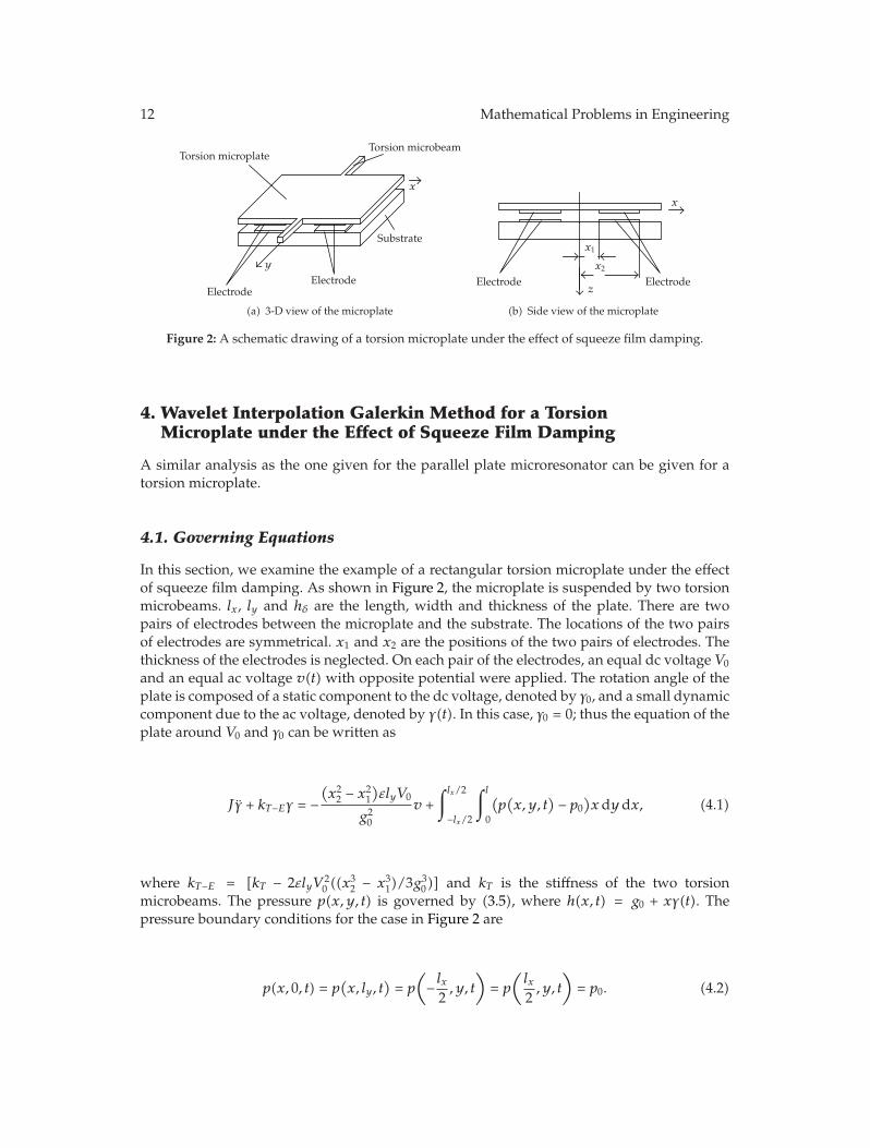
Figure 2: A schematic drawing of a torsion microplate under the effect of squeeze film damping.

4. Wavelet Interpolation Galerkin Method for a TorsionMicroplate under the Effect of Squeeze Film Damping

A similar analysis as the one given for the parallel plate microresonator can be given for atorsion microplate.

4.1. Governing Equations

In this section, we examine the example of a rectangular torsion microplate under the effectof squeeze film damping. As shown in Figure 2, the microplate is suspended by two torsionmicrobeams. lx, ly and hδ are the length, width and thickness of the plate. There are twopairs of electrodes between the microplate and the substrate. The locations of the two pairsof electrodes are symmetrical. x1 and x2 are the positions of the two pairs of electrodes. Thethickness of the electrodes is neglected. On each pair of the electrodes, an equal dc voltage V0

and an equal ac voltage v(t) with opposite potential were applied. The rotation angle of theplate is composed of a static component to the dc voltage, denoted by γ0, and a small dynamiccomponent due to the ac voltage, denoted by γ(t). In this case, γ0 = 0; thus the equation of theplate around V0 and γ0 can be written as

Jγ + kT−Eγ = −(x2

2 − x21

)εlyV0

g20

v +∫ lx/2

−lx/2

∫ l

0

(p(x, y, t

)− p0)xdy dx, (4.1)

where kT−E = [kT − 2εlyV 20 ((x

32 − x3

1)/3g30)] and kT is the stiffness of the two torsion

microbeams. The pressure p(x, y, t) is governed by (3.5), where h(x, t) = g0 + xγ(t). Thepressure boundary conditions for the case in Figure 2 are

p(x, 0, t) = p(x, ly, t

)= p(− lx

2, y, t

)= p(lx2, y, t

)= p0. (4.2)


For convenience, we introduce the nondimensional variables

X =x

lx+

12, X1 =

x1

lx+

12, X2 =

x2

lx+

12, Y =

y

ly, ϑ =

γ

γmax, γmax =

2g0

lx,

P =p

p0, T =

t

S, H =

h

g0= 1 + 2

(X − 1

2

)ϑ,

(4.3)

where S =√J/(kT−E) = 1/ωn, ωn is the nature frequency of the plate. Substituting (4.3) into

(4.1), (3.5) and (4.2), we obtain

ϑ + ϑ = −αV0v + Pnon

∫∫1

0

(P(X,Y, T) − 1

)(X − 1

2

)dX dY, (4.4)

∂

∂X

(H3P

∂P

∂X

)+ β2 ∂

∂Y

(H3P

∂P

∂Y

)=σ

S

(H∂P

∂T+ P

∂H

∂T

), (4.5)

where α = (x22−x

21)εly/kT−Eg

20γmax, Pnon = p0l

2xly/kT−eγmax, σ = 12ηl2x/g

20p0, and β = lx/ly. The

nondimensional boundary conditions are

P(X, 0, T) = P(X, 1, T) = P(0, Y, T) = P(1, Y, T) = 1. (4.6)

As mentioned above, the microplate is under small torsion oscillation around γ0 = 0and therefore the pressure variation from ambient in the squeeze film is also small, P(X,Y, T)is given by

P(X,Y, T) =p

p0= 1 + P(X,Y, T), (4.7)

where |P(X,Y, T)| 1. Substituting (4.7) into (4.5), and linearizing the outcome around p0

and γ0, we obtain

∂2P

∂X2+ β2 ∂

2P

∂Y 2− σS

∂P

∂T=

2σS

(X − 1

2

)∂ϑ

∂T. (4.8)

The boundary conditions for the case are

P(X, 0, T) = P(X, 1, T) = P(0, Y, T) = P(1, Y, T) = 0. (4.9)

For a harmonic excitation, the ac component voltage v(T) is given by

v(T) = v0ejωTS. (4.10)


Correspondingly, the steady-state solution of (4.4) and (4.8) may be expressed by

ϑ(T) = AejωTS,

P(X,Y, T) = A · PA(X,Y )ejωTS,(4.11)

where A is the complex amplitude to be determined. Substituting (4.11) into (4.8), we obtain

∂2PA(X,Y )∂X2

+ β2 ∂2PA(X,Y )∂Y 2

− jσωPA(X,Y ) = j2σω(X − 1

2

). (4.12)

The boundary conditions are

PA(X, 0) = PA(X, 1) = PA(0, Y ) = PA(1, Y ) = 0. (4.13)

4.2. Wavelet Interpolation Method for Squeeze Film Damping Equations

In this section, the approximate solution of PA(X,Y ) can be approximated by (3.21). The weakform functional of (4.12) is

W(PA) =∫∫

Ω

{12

[(∂PA∂X

)2

+ β2(∂PA∂Y

)2

+ jσωP 2A

]+ j2σω

(X − 1

2

)PA

}dX dY. (4.14)

From the necessary conditions for the determination of the minimum W , we obtain

δW(PA) =∫∫

Ω

[∂δPA∂X

∂PA∂X

+ β2 ∂δPA∂Y

∂PA∂Y

+ jσωδPAPA + j2σω(X − 1

2

)δPA

]dX dY = 0.

(4.15)


2J−1∑

k=1

2J−1∑

k′=1

⎧⎨

⎩

∫∫

Ω

⎡

⎣∂ΘJm,n

∂X

∂ΘJk,k′

∂X+ β2 ∂Θ

Jm,n

∂Y

∂ΘJk,k′

∂Y+ jσωΘJ

m,nΘJk,k′

⎤

⎦dX dY

⎫⎬

⎭pJk,k′

= −j2σω∫∫

Ω

(X − 1

2

)ΘJm,ndX dY, for m,n = 1, 2, . . . ,

(2J − 1

).

(4.16)

This is a(2J − 1

)2 ×(2J − 1

)2 linear system

Θp = −jσωE, (4.17)

where p=[pJ1,1 p

J1,2 · · · p

J

1,2J−1 pJ2,1 p

J2,2 · · · p

J

2J−1,2J−1

]Tis an

(2J − 1

)2 × 1 unknown coefficients’

matrix, E=2[∫∫

Ω(X−1/2)ΘJ1,1dX dY

∫∫Ω(X−1/2)ΘJ

1,2dX dY · · ·∫∫

Ω(X−(1/2))ΘJ

2J−1,2J−1dXdY]T


is a(2J − 1

)2 × 1 matrix, and Θ is a(2J − 1

)2 ×(2J − 1

)2 matrix. The entries in Θ are of theform

Θ(i, j)= Θ([

(m − 1)(

2J − 1)+ n],[(k − 1)

(2J − 1

)+ k′])

=∫∫

Ω

[∂θ(2JX −m

)

∂Xθ(

2JY − n)∂θ(2JX − k

)

∂Xθ(

2JY − k′)

+ β2θ(

2JX −m)∂θ(2JY − n

)

∂Yθ(

2JX − k)∂θ(2JY − k′

)

∂Y

+jσωθ(

2JX −m)θ(

2JY − n)θ(

2JX − k)θ(

2JY − k′)]

dX dY.

(4.18)

4.2.1. Squeeze Film Damping of the Torsion Plate

The numerical solution of (4.17) can be written as

p = −jσωΘ−1E. (4.19)

The elements of p can be expressed as

pJk,k′ = −p

J,Rk,k′ − jp

J,Ik,k′ for m,n = 1, 2, . . . ,

(2J − 1

), (4.20)

where pJ,Rk,k′

and pJ,Ik,k′

are the real and imaginary parts of pJk,k′

, respectively. Using (4.20) and(4.4), the force acting on the plate owing to the pressure of the squeeze gas film can berewritten as

Pnon

∫∫1

0

(P − 1

)(X − 1

2

)dX dY = −Ka · ϑ(T) − Ca ·

dϑ(T)dT

, (4.21)

where Ka · ϑ(T) and Ca · (dϑ(T)/dT) are the spring and damping components of the force

Ka = Pnon

2J−1∑

k=1

2J−1∑

k′=1

pJ,Rk,k′

∫∫1

0θ(

2JX − k)θ(

2JY − k′)(

X − 12

)dX dY

Ca =Pnon

ωS

2J−1∑

k=1

2J−1∑

k′=1

pJ,Ik,k′

∫∫1

0θ(

2JX − k)θ(

2JY − k′)(

X − 12

)dX dY

(4.22)


Table 1: The parameters of the accelerometer presented by Veijola et al. [26].

Parameters ValuesMass mplate 4.9 × 10−6 kgSpring constant kspring 212.1 N/mGap spacing g0 3.95μmLength of the moving masss lx 2 960μmWidth of the moving masss ly 1 780μmAmbient pressure p0 11 PaBias voltage V0 9 VEffective viscosity ηeff 10.2 × 10−9 N·s·m−2


d2ϑ

dT2+ Ca ·

dϑ

dT+ (Ka + 1)ϑ = αV0v(T),

ϑ(T) = AejωTS =aV0v0

Ka + 1· 1

1 − (ω2(S2/(Ka + 1))) +(jω(CaS/(Ka + 1))

)ejωTS.(4.23)

The quality factor and the damped natural frequency are given in(3.32)

5. Comparisons with Experiments

Veijola et al. [26] conducted experiments to measure the frequency response of anaccelerometer under the effect of squeeze film damping. Minikes et al. [27] measuredthe quality factors of two torsion rectangular mirrors at low pressure. In this section, theexperimental results presented by Veijola et al. [26] and Minikes et al. [27] were used toverify the wavelet interpolation Galerkin method.

5.1. Comparisons with the Experimental Results of Veijola et al. [26]

In [26], Veijola et al. simulated the frequency response of an accelerometer with a spring-mass- damper model with a parallel-plate electrostatic force. The damping coefficient wasestimated by the Blech model [28]. The spring constants and the gas pressures were estimatedby curve fitting the experimental measurements. They compared their simulations withexperimental data and found good agreement. The parameters for the accelerometer are listedin Table 1.

In this subsection, we use the wavelet interpolation Galerkin method to predict thefrequency response of the accelerometer. Various numerical tests have been conducted bychanging the degree of the Daubechies wavelet L and the number J of the scale. Betteraccuracy can be achieved by increasing L and J . The higher L is, the smoother the scalingfunction becomes. The price for the high smoothness is that its supporting domain gets larger.The higher J is, the more accurate the solution becomes. The number of differential equationsand the CPU time increase significantly as J increases. In this work, only the solutions forL = 6 and J = 4 are presented, as the results for higher resolutions are indistinguishable fromthe exact solution.


For comparison purpose, we give the frequency responses of the accelerometercalculated by Blech’s model [28] and the finite difference method, respectively. Blech [28]expanded the air film pressure into an assumed double sine series and derived an analyticalexpression for the spring and damping forces. In this subsection, the number of terms for thedouble sine series is taken as (5, 5), which shows good convergence. For the finite differencemethod, we use the following approximate formulae for a node (i, j) on the microplate:

∂PA∂X

∣∣∣∣i,j

=PA(i + 1, j

)− PA

(i − 1, j

)

2ΔX,

∂PA∂Y

∣∣∣∣i,j

=PA(i, j + 1

)− PA

(i, j − 1

)

2ΔY,

∂2PA∂X2

∣∣∣∣∣i,j

=PA(i + 1, j

)− 2PA

(i, j)+ PA

(i − 1, j

)

Δ2X

,

∂2PA∂Y 2

∣∣∣∣∣i,j

=PA(i, j + 1

)− 2PA

(i, j)+ PA

(i, j − 1

)

Δ2Y

.

(5.1)

In this subsection, we assume that ΔX = ΔY = 1/2J = 1/26; thus the element size of the finitedifference method is equal to the wavelet interpolation Galerkin method. Substituting (5.1)into (3.17), we obtain

PA(i + 1, j

)+ PA

(i − 1, j

)+ β2PA

(i, j + 1

)+ β2PA

(i, j − 1

)

Δ2X

−(

2 + 2β2

Δ2X

+ jσω

)PA(i, j)= −jσω.

(5.2)

Figure 3 shows the comparisons of the frequency response obtained by differentmethods. As expected, the wavelet interpolation Galerkin method, Blech’s model andthe finite difference method give almost same results. The three results agree well withthe experimental results [26] except for one data at resonance peak of the amplitudefrequency response. The reason for this discrepancy is that the damping coefficient isslightly underestimated by the three methods, respectively. Table 2 shows the Comparisonof the damping obtained by different methods. In the experiment [26], the squeeze filmdamping is dominant. Obviously, the accuracy of the finite difference method is less thanthe wavelet interpolation Galerkin method and Blech’s model. The wavelet interpolationGalerkin method and the Blech model give almost identical results. Figure 4 shows the realpart and the imaginary part of the air film pressure calculated by the wavelet interpolationGalerkin method.

5.2. Comparisons with the Experimental Results of Minikes et al. [27]

Minikes et al. [27] measured the quality factors of two rectangular torsion mirrors at lowpressure and plotted the curves of the quality factors as a function of air pressure in therange from 10−2 torr to 102 torr. The structure of the two torsion mirrors is identical withthe structure shown in Figure 2. The two torsion mirrors have similar dimensions in terms


−50

−40

−30

−20

−10

0

10

20

30

Am

plit

ude(d

B)

102 103 104

Frequency (Hz)

(a) Amplitude response

−180

−160

−140

−120

−100

−80

−60

−40

−20

0

20

Phas

e

102 103 104

Frequency (Hz)

Experimental data [26]Blech’s modelThe finite difference methodThe wavelet interpolation Galerkin method

(b) Phase response

Figure 3: Comparisons of the frequency response obtained by the wavelet Galerkin method, the Blechmodel and the experimental data of Veijola et al. [26].


0

0.2

0.4

0.6

0.8R

ealp

arto

fPA

10.5

X 0 0

0.5

Y

1

(a) The real part of the pressure distribution

0

0.2

0.4

0.6

0.8

Imag

inar

ypa

rtofPA

10.5

X0 0

0.5

Y

1

(b) The imaginary part of the pressure distribution

Figure 4: The air film pressure distribution calculated by the wavelet interpolation Galerkin method.

Table 2: A Comparison of the damping ratios obtained by different methods with the experimental data[26].

Methods Damping ratio Peak value (dB)Experimental data [26] 0.0239 18.3Blech’s model (error) 0.0159 (33.5%) 21.7The wavelet interpolation Galerkin method (error) 0.0155 (35.1%) 21.9The finite difference method (error) 0.0136 (43.1%) 23.2

of surface area and inertial moment, but have different gaps between the mirror and theactuation electrodes. The parameters for the two torsion mirrors are listed in Table 3.

In Table 3, the values of the two torsional natural frequencies are measured underthe dc bias voltage. Based on the two torsional natural frequencies and two moments ofinertia, we determined the torsional stiffness kT−E. The extracted torsional stiffness kT−Efor mirror 1 and mirror 2 are 2.461 × 10−6 and 2.362 × 10−6 N·m/rad, respectively. Nowwe use the wavelet interpolation Galerkin method to predict the quality factors of the twotorsion mirrors. Various numerical tests have been conducted by changing the degree of theDaubechies wavelet L and the number J of the scale. Only the solutions for L = 6 and J = 4 arepresented, as the results for higher resolutions are indistinguishable from the exact solution.

For comparison purpose, we give the quality factors calculated by Pan’s model [15]and the finite difference method, respectively. Pan et al. [15] expanded the air film pressureinto an assumed double sine series and derived an analytical expression for the spring anddamping torques. In this work, the number of terms for the double sine series is taken as(6, 5), which shows good convergence. For the finite difference method, we use (5.1) and(4.12) for a node (i, j) on the mirror; thus obtain

PA(i + 1, j

)+ PA

(i − 1, j

)+ β2PA

(i, j + 1

)+ β2PA

(i, j − 1

)

Δ2X

−(

2 + 2β2

Δ2X

+ jσω

)PA(i, j)

= j2σω(Xi −

12

).

(5.3)


Table 3: The parameters of two torsion mirrors [27].

Mirror 1 Mirror 2Width of the mirror ly 500μm 500μmLength of the mirror lx 500μm 500μmThickness of the mirror hδ 30μm 30μmDensity of the mirror ρ 2300 kg/m3 2300 kg/m3

Gap spacing g0 28μm 13μmTorsional natural frequency fn 13092.56 Hz 12824.87 Hz

Table 4: A comparison of quality factors obtained by Pan’s model, the wavelet interpolation Galerkinmethod and the finite difference method for mirror 1.

p0 (torr) Pan’s model

The waveletinterpolation

Galerkin method(error)

The finite differencemethod (error)

0.08 5.784 × 104 5.987 × 104 (3.5%) 6.586 × 104 (13.9%)0.10 4.483 × 104 4.627 × 104 (3.2%) 5.160 × 104 (15.1%)0.50 7.070 × 103 7.330 × 103 (3.7%) 8.006 × 103 (13.2%)1 3.306 × 103 3.388 × 103 (2.5%) 3.694 × 103 (11.7%)3 1.061 × 103 1.080 × 103 (1.8%) 1.173 × 103 (10.6%)6 5.680 × 102 5.895 × 102 (3.8%) 6.526 × 102 (14.9%)10 3.979 × 102 4.052 × 102 (1.8%) 4.454 × 102 (11.9%)30 2.451 × 102 2.505 × 102 (2.2%) 2.721 × 102 (11.0%)60 2.074 × 102 2.160 × 102 (4.1%) 2.327 × 102 (12.2%)100 1.994 × 102 2.035 × 102 (2.1%) 2.240 × 102 (12.3%)760 1.850 × 102 1.896 × 102 (2.5%) 2.109 × 102 (14.0%)

In this subsection, we assume that ΔX = ΔY = 1/2J = 1/26; thus the finite difference methodyields the same grids as the wavelet interpolation Galerkin method.

Tables 4 and 5 show the comparisons of quality factors obtained by the waveletinterpolation Galerkin method, the finite difference method and Pan’s model for the mirror1 and 2, respectively. As shown in Tables 4 and 5, the qualify factors obtained by the waveletinterpolation Galerkin method are almost 1% ∼4% higher than Pan’s model. However thequalify factors obtained by the finite difference method are almost 10% ∼15% higher thanPan’s model. The result of the wavelet interpolation Galerkin method matches the result ofPan’s model better than that of the finite difference method.

Figure 5 shows the comparisons of quality factors obtained by different methods. Asexpected, the wavelet interpolation Galerkin method, the finite difference method and Pan’smodel give almost same results. Above p0 = 10 torr, the viscous damping is dominant, thethree methods give results in good agreement with the experimental results [27]. Below p0

= 10 torr, the accuracy of the three methods decreases as the pressure decreases. The mainreason for this trend are as follows. The three methods are based on Reynolds equation,which is derived from the Navier-Stokes equations and the continuity equation. The mainassumption is that the gas in the gap can be treated as a continuum. Below p0 = 10 torr, theKnudsen number Kn > 0.1, the gas in the gap cannot be treated as a continuum. Thus thethree methods fail to give a good prediction. Below p0 = 0.1 torr, the influence of squeeze film


101

102

103

104

105

Qua

lity

fact

orQ

10−2 100 102

Pressure (torr)

(a) Mirror 1 (g0= 28μm)

101

102

103

104

105

Qua

lity

fact

orQ

10−2 100 102

Pressure (torr)

Experimental data [27]Pan’s modelThe finite difference methodThe wavelet interpolation Galerkin method

(b) Mirror 2 (g0= 13μm)

Figure 5: Comparison of the quality factors obtained by the wavelet Galerkin method, the Pan model andthe experimental data of Minikes et al. [27].

damping begins to vanish and the qualify factors reaches a plateau that is dominated by theintrinsic damping.

Tables 6 and 7 list the comparisons of quality factors between p = 10 and 760 torr formirrors 1 and 2, respectively. Obviously, the accuracy of the finite difference method is lessthan the wavelet interpolation Galerkin method and Pan’s model. Figure 6 shows the real


−3

−2

−1

0

1

2

3×10−3

Rea

lpar

tofP

A

10.5X

0 00.5

Y

1

(a) The real part of mirror 1

−0.04

−0.02

0

0.02

0.04

Imag

inar

ypa

rtofPA

10.5

X0 0

0.5Y

1

(b) The imaginary part of mirror 1

−0.01

−0.005

0

0.005

0.01

Rea

lpar

tofP

A

10.5

X0 0

0.5

Y

1

(c) The real part of mirror 2

−0.1

−0.05

0

0.05

0.1

Imag

inar

ypa

rtofPA

10.5

X0 0

0.5

Y

1

(d) The imaginary part of mirror 2

Figure 6: The air film pressure distribution calculated by the wavelet interpolation Galerkin method at p0= 1 torr.

Table 5: A comparison of quality factors obtained by Pan’s model, the wavelet interpolation Galerkinmethod and the finite difference method for mirror 2.

p0 (torr) Pan’s model


Galerkin method(error)

The finite differencemethod (error)

0.08 1.645 × 104 1.679 × 104 (2.1%) 1.847 × 104 (12.3%)0.10 1.268 × 104 1.297 × 104 (2.3%) 1.458 × 104 (15.0%)0.50 2.135 × 103 2.208 × 103 (3.4%) 2.352 × 103 (10.2%)1 8.919 × 102 9.195 × 102 (3.1%) 1.010 × 103 (13.2%)3 2.681 × 102 2.712 × 102 (1.2%) 3.012 × 102 (12.3%)6 1.282 × 102 1.318 × 102 (2.8%) 1.463 × 102 (14.1%)10 8.004 × 101 8.118 × 101 (1.4%) 9.092 × 101 (13.6%)30 3.461 × 101 3.599 × 101 (4.0%) 3.959 × 101 (14.4%)60 2.574 × 101 2.628 × 101 (2.1%) 2.970 × 101 (15.4%)100 2.255 × 101 2.278 × 101 (1.0%) 2.593 × 101 (15.0%)760 1.820 × 101 1.900 × 101 (4.4%) 2.055 × 101 (12.9%)


Table 6: A comparison of quality factors between p0 = 10 and 760 torr for mirror 1.

p0 (torr) Experiment data [27] Pan’s model (error)


Galerkinmethod(error)

The finitedifferencemethod(error)

10 345 398 (15.4%) 405 (17.4%) 445 (29.0%)20 275 289 (5.1%) 301 (9.4%) 311 (13.1%)40 229 236 (3.1%) 241 (5.2%) 252 (10.0%)760 179 185 (3.4%) 190 (6.1%) 211 (17.9%)

Table 7: A comparison of quality factors between p0 = 10 and 760 torr for mirror 2.

p0 (torr) Expertiment data [27] Pan’s model (error)


Galerkinmethod(error)

The finitedifferencemethod(error)

10 66 80.0 (21.2%) 81.2 (23.0%) 90.9 (37.7%)20 40 48.8 (22.0%) 50.1 (25.3%) 54.0 (35.0%)40 27 30.1 (11.5%) 31.0 (14.8%) 33.5 (24.1%)760 18 18.2 (1.1%) 19.0 (5.6%) 20.6 (14.4%)

part and the imaginary part of the air film pressure calculated by the wavelet interpolationGalerkin method at p0 = 1 torr. The air film pressure looks similar to the results calculated byPan’s model.

6. Summary and Conclusions

A new wavelet interpolation Galerkin method has been developed for the numericalsimulation of MEMS devices under the effect of squeeze film damping. The air film pressureare expressed as a linear combination of a class of interpolating functions generated byautocorrelation of the usual compactly supported Daubechies scaling functions. To the bestof our knowledge, this is the first time that wavelets have been used as basis functions forsolving the PDEs of MEMS devices. As opposed to the previous wavelet-based methods thatare all limited in one energy domain, the MEMS devices in the paper involve two coupledenergy domains. Two typical electrically actuated micro devices with squeeze film dampingeffect are examined respectively to illustrate the wavelet interpolation Galerkin method. Themethod is validated by comparing its results with available theoretical and experimentalresults. The accuracy of the method is higher than the finite difference method.

In this paper, the wavelet interpolation Galerkin method is not suitable to solveproblems defined on nonrectangular domains, since higher-dimensional wavelets areconstructed by employing the tensor product of the one-dimensional wavelets and so theirapplication is restricted to rectangular domains. In this paper, both trial and weight functionsare a class of interpolating functions generated by autocorrelation of the first-generationwavelets. Future area of research is based on the second-generation wavelets [29]. The main


advantage of the second-generation wavelets is that the wavelets are constructed in thespatial domain and can be custom designed for complex domains. This work is currentlyunder way.

Acknowledgments

This work was supported by the National Natural Science Foundation of China (Grants No.60806036 and 50675034), the Natural Science Foundation of Jiangsu Province (Grant No.BK2009286), and Natural Science Research Plan of the universities in Jiangsu Province (GrantNo. 08KJB510014).

References

[1] A. H. Nayfeh, M. I. Younis, and E. M. Abdel-Rahman, “Reduced-order models for MEMSapplications,” Nonlinear Dynamics, vol. 41, no. 1–3, pp. 211–236, 2005.

[2] E. S. Hung and S. D. Senturia, “Generating efficient dynamical models for microelectromechanicalsystems from a few finite-element simulation runs,” Journal of Microelectromechanical Systems, vol. 8,no. 3, pp. 280–289, 1999.

[3] A. H. Nayfeh and M. I. Younis, “A new approach to the modeling and simulation of flexiblemicrostructures under the effect of squeeze-film damping,” Journal of Micromechanics and Microengi-neering, vol. 14, no. 2, pp. 170–181, 2004.

[4] M. I. Younis, E. M. Abdel-Rahman, and A. Nayfeh, “A reduced-order model for electrically actuatedmicrobeam-based MEMS,” Journal of Microelectromechanical Systems, vol. 12, no. 5, pp. 672–680, 2003.

[5] E. M. Abdel-Rahman, M. I. Younis, and A. H. Nayfeh, “Characterization of the mechanical behaviorof an electrically actuated microbeam,” Journal of Micromechanics and Microengineering, vol. 12, no. 6,pp. 759–766, 2002.

[6] Y. C. Liang, W. Z. Lin, H. P. Lee, S. P. Lim, K. H. Lee, and H. Sun, “Proper orthogonal decompositionand its applications—part II: model reduction for MEMS dynamical analysis,” Journal of Sound andVibration, vol. 256, no. 3, pp. 515–532, 2002.

[7] Y. C. Liang, W. Z. Lin, H. P. Lee, S. P. Lim, K. H. Lee, and D. P. Feng, “A neural-network-basedmethod of model reduction for the dynamic simulation of MEMS,” Journal of Micromechanics andMicroengineering, vol. 11, no. 3, pp. 226–233, 2001.

[8] W. Z. Lin, K. H. Lee, S. P. Lim, and Y. C. Liang, “Proper orthogonal decomposition and componentmode synthesis in macromodel generation for the dynamic simulation of a complex MEMS device,”Journal of Micromechanics and Microengineering, vol. 13, no. 5, pp. 646–654, 2003.

[9] P. Li, R. Hu, and Y. Fang, “A new model for squeeze-film damping of electrically actuated microbeamsunder the effect of a static deflection,” Journal of Micromechanics and Microengineering, vol. 17, no. 7,pp. 1242–1251, 2007.

[10] L. D. Gabbay, J. E. Mehner, and S. D. Senturia, “Computer-aided generation of nonlinear reduced-order dynamic macromodels—I: non-stress-stiffened case,” Journal of Microelectromechanical Systems,vol. 9, no. 2, pp. 262–269, 2000.

[11] J. E. Mehner, L. D. Gabbay, and S. D. Senturia, “Computer-aided generation of nonlinear reduced-order dynamic macromodels—II: stress-stiffened case,” Journal of Microelectromechanical Systems, vol.9, no. 2, pp. 270–278, 2000.

[12] M. I. Younis and A. H. Nayfeh, “Simulation of squeeze-film damping of microplates actuated by largeelectrostatic load,” Journal of Computational and Nonlinear Dynamics, vol. 2, no. 3, pp. 232–241, 2007.

[13] C. Zhang, G. Xu, and Q. Jiang, “Characterization of the squeeze film damping effect on the qualityfactor of a microbeam resonator,” Journal of Micromechanics and Microengineering, vol. 14, no. 10, pp.1302–1306, 2004.

[14] A. K. Pandey and R. Pratap, “Effect of flexural modes on squeeze film damping in MEMS cantileverresonators,” Journal of Micromechanics and Microengineering, vol. 17, no. 12, pp. 2475–2484, 2007.

[15] F. Pan, J. Kubby, E. Peeters, A. T. Tran, and S. Mukherjee, “Squeeze film damping effect on the dynamicresponse of a MEMS torsion mirror,” Journal of Micromechanics and Microengineering, vol. 8, no. 3, pp.200–208, 1998.


[16] I. Daubechies, Ten Lectures on Wavelets, vol. 61 of CBMS-NSF Regional Conference Series in AppliedMathematics, SIAM, Philadelphia, Pa, USA, 1992.

[17] S. Mallat, A Wavelet Tour of Signal Processing, Academic Press, San Diego, Calif, USA, 1998.[18] M.-Q. Chen, C. Hwang, and Y.-P. Shih, “The computation of wavelet-Galerkin approximation on a

bounded interval,” International Journal for Numerical Methods in Engineering, vol. 39, no. 17, pp. 2921–2944, 1996.

[19] S. L. Ho and S. Y. Yang, “Wavelet-Galerkin method for solving parabolic equations in finite domains,”Finite Elements in Analysis and Design, vol. 37, no. 12, pp. 1023–1037, 2001.

[20] S. Yang, G. Ni, J. Qiang, and R. Li, “Wavelet-Galerkin method for computations of electromagneticfields,” IEEE Transactions on Magnetics, vol. 34, no. 5, part 1, pp. 2493–2496, 1998.

[21] S. Bertoluzza and G. Naldi, “A wavelet collocation method for the numerical solution of partialdifferential equations,” Applied and Computational Harmonic Analysis, vol. 3, no. 1, pp. 1–9, 1996.

[22] Y. Liu, I. T. Cameron, and F. Y. Wang, “The wavelet-collocation method for transient problems withsteep gradients,” Chemical Engineering Science, vol. 55, no. 9, pp. 1729–1734, 2000.

[23] Y.-H. Zhou and J. Zhou, “A modified wavelet approximation for multi-resolution AWCM insimulating nonlinear vibration of MDOF systems,” Computer Methods in Applied Mechanics andEngineering, vol. 197, no. 17-18, pp. 1466–1478, 2008.

[24] W. Yan, X. Shen, and L. Shi, “A wavelet interpolation galerkin method for the numerical solution ofPDEs in 2D magnetostatic field,” IEEE Transactions on Magnetics, vol. 36, no. 4, part 1, pp. 639–643,2000.

[25] Y. Y. Kim and G.-W. Jang, “Hat interpolation wavelet-based multi-scale Galerkin method for thin-walled box beam analysis,” International Journal for Numerical Methods in Engineering, vol. 53, no. 7,pp. 1575–1592, 2002.

[26] T. Veijola, H. Kuisma, J. Lahdenpera, and T. Ryhanen, “Equivalent-circuit model of the squeeze gasfilm in a silicon accelerometer,” Sensors and Actuators A, vol. 48, pp. 239–248, 1995.

[27] A. Minikes, I. Bucher, and G. Avivi, “Damping of a micro-resonator torsion mirror in rarefied gasambient,” Journal of Micromechanics and Microengineering, vol. 15, no. 9, pp. 1762–1769, 2005.

[28] J. J. Blech, “On isothermal squeeze films,” Journal of Lubrication Technology A, vol. 105, no. 4, pp. 615–620, 1983.

[29] O. V. Vasilyev and C. Bowman, “Second-generation wavelet collocation method for the solution ofpartial differential equations,” Journal of Computational Physics, vol. 165, no. 2, pp. 660–693, 2000.

a wavelet interpolation galerkin method for the...

Documents