University of California, Davis

Atmospheric Boundary Layer Wind Tunnel Facility Department of Mechanical and Aeronautical Engineering

One Shields Avenue, Davis, California 95616-5294

FINAL REPORT A WIND-TUNNEL MODEL OF WIND EFFECTS ON AN AIR COOLING CONDENSER Bruce R. White, Professor Daeseong Kim, Research Manager John Christopher Bachman, Undergraduate Associate

Prepared for :

Electric Power Research Institute 3420 Hillview Avenue, P.O. Box 10412,

Palo Alto, California 94303

December 2009

TABLE OF CONTENTS

TABLE OF CONTENTS................................................................................................................ 2

INTRODUCTION .......................................................................................................................... 3

WIND TUNNEL MODELING ...................................................................................................... 7

Atmospheric Flow Similarity...................................................................................................... 7

Boundary Layer Similarity ....................................................................................................... 10

Scaled Model Design and Construction.................................................................................... 14

TESTING FACILITIES................................................................................................................ 20

The Atmospheric Boundary Layer Wind Tunnel at UC Davis................................................. 20

Instrumentation and Measurement System............................................................................... 22

TESTING METHODOLOGY...................................................................................................... 25

SINGLE UNIT MODEL ANALYSIS.......................................................................................... 34

Wind-tunnel Testing Results..................................................................................................... 34

Application of Meteorological Data ......................................................................................... 40

Individual Contribution of Fan Cells ........................................................................................ 42

Mitigation Plans ........................................................................................................................ 44

DUAL UNIT MODEL ANALYSIS............................................................................................. 52

CONCLUSION............................................................................................................................. 56

ACKNOWLEDGEMENTS.......................................................................................................... 57

REFERENCES ............................................................................................................................. 58

APPENDIX................................................................................................................................... 60

Appendix –A Testing Results of the Single Unit Base Model ................................................. 60

Appendix – B Testing Results of the Dual Unit Base Model .................................................. 82

2

INTRODUCTION

There will be increasing competition for fresh water supplies in the future, due to several

key demographic, technical, and regulatory factors. These factors include; (1) rapid population

growth in the United States (U.S.), particularly in the southwestern states; (2) the resulting

growth of electricity demand and water consumption for power generation and other uses; (3)

periodic drought conditions that may increase in severity as a result of global climate change;

and, (4) regulatory requirements that limit thermal emissions and restrict both water supplies and

effluent quality. Since the water consumption of thermoelectric power plants and the electricity

demand are highly linked, it is imperative to develop a new power plant that can effectively

utilize a minimal amount of water.

Thermoelectric power plants, such as nuclear, and many types of fossil fuel plants are

equipped with a cooling system. Typical and efficient cooling systems include a once-through

cooling system and an evaporative wet cooling tower. However, once-through cooling systems

withdraw significant volumes of water to cool the condenser and is subject to Sections 316a

(thermal) and 316b (fish impingement and entrainment) of the U.S. Clean Water Act. Wet

cooling towers consume 85% to 90% of the water withdrawn via evaporation and would be

unfavorable in a water-constrained environment. The direct dry cooling systems are somewhat

less effective than once-through cooling systems, although are a good alternative when trying to

minimize water consumption.

An air cooling condenser (ACC) is the core of any direct dry cooling system. The air

cooling condenser shown in Figure 1 uses space saving A-frame fin tubes. The steam exhausted

from the turbine flows through the steam header on top of the A-frame and then flows diagonally

down through finned tubes. Cool air is then drawn by fan units upward across the heat

exchanging tubes and condenses the steam. In a typical ACC system, a significant number of

these fans and A-frame fin tubes are usually installed on a rectangular platform hundreds of feet

above the ground. The number of fans and tubes depends on the plant’s capacity. The ACC

platform can be installed on the top of the boiler house, if the plant is small. At large power

plants, the ACC platforms are located near the boiler house in various forms: single line, two

lines, or in two-dimensional grid formations.

3

Figure 1 Schematic Drawing of an Air Cooling Condenser Cell

Under stable conditions with no wind, the backpressure can be easily controlled by

changing the air flow rate through the ACC unit. In reality, the wind blows a majority of the

time and a number of studies have argued that the wind, in general, negatively affects the

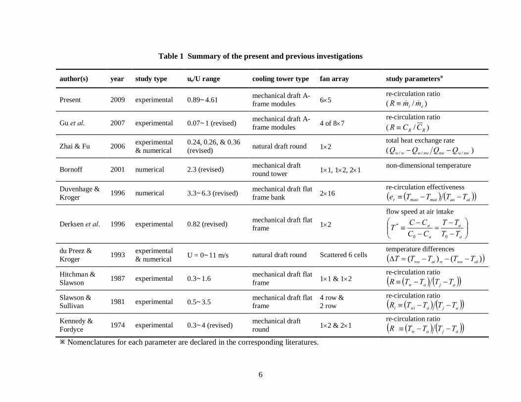
performance of ACC systems. As it is shown in Table-1, many experimental and computational

studies have investigated the wind effects on ACC systems and the possible mitigation plans.

However, an investigation of practical wind effect is scarce due to the ACC unit’s site specific

meteorological conditions. The varying meteorological conditions make it impractical to apply

one case to another.

The objective of the present study is to physically model an air cooling condenser and to

assess potential mitigation measures to reduce the impact of the wind on the ACC’s performance.

The present study supports Electric Power Research Institute (EPRI)’s participation in the

Electricite de France-EPRI Advanced Cooling Technology Partnership, which is to assess and

develop advanced power plant cooling technology concepts for a water-constrained future. A

parallel contract will extend EPRI report 1005358, “Comparison of Alternative Cooling

Technologies for U.S. Power Plants: Economic, Environmental, and Other Tradeoffs,” to nuclear

4

5

power plants and evaluates advanced power plant cooling concepts for thermoelectric power

plants.

The work scope of the present study includes: (1) development and construction of

simplified scale models of power plants with both single-unit and dual-unit ACCs; (2) wind-

tunnel testing of the scale models to assess high wind impacts on air-flow around and within

ACC cells; (3) wind-tunnel testing of mitigation measures to reduce wind impacts on ACC

performance; and, (4) applying the field data to the wind tunnel study results.

author(s) year study type ue/U range cooling tower type fan array study parameters

Present 2009 experimental 0.89~4.61 mechanical draft A-frame modules 6×5

re-circulation ratio ( ei mmR && /≡ )

Gu et al. 2007 experimental 0.07~1 (revised) mechanical draft A-frame modules 4 of 8×7

re-circulation ratio ( RR CCR /≡ )

Zhai & Fu 2006 experimental & numerical

0.24, 0.26, & 0.36 (revised) natural draft round 1×2

total heat exchange rate ( nwwnwnwwww QQQQ /// −− )

Bornoff 2001 numerical 2.3 (revised) mechanical draft round tower 1×1, 1×2, 2×1 non-dimensional temperature

Duvenhage & Kroger 1996 numerical 3.3~6.3 (revised) mechanical draft flat

frame bank 2×16 re-circulation effectiveness

( ) ( )( )aiaomaimaor TTTTe −−≡

Derksen et al. 1996 experimental 0.82 (revised) mechanical draft flat frame 1×2

flow speed at air intake

⎟⎟⎠

⎞⎜⎜⎝

⎛−−

=−−

≡a

a

a

a

TTTT

CCCCT

00

*

du Preez & Kroger 1993 experimental

& numerical U = 0~11 m/s natural draft round Scattered 6 cells temperature differences ( ))()( aiwowaiwo TTTTT −−−=∆

Hitchman & Slawson 1987 experimental 0.3~1.6 mechanical draft flat

frame 1×1 & 1×2 re-circulation ratio

( ) ( )( )ajaw TTTTR −−≡

Slawson & Sullivan 1981 experimental 0.5~3.5 mechanical draft flat

frame 4 row & 2 row

re-circulation ratio ( ) ( )( )ajawii TTTTR −−≡

Kennedy & Fordyce 1974 experimental 0.3~4 (revised) mechanical draft

round 1×2 & 2×1 re-circulation ratio

( ) ( )( )ajaw TTTTR −−≡

Nomenclatures for each parameter are declared in the corresponding literatures.

Table 1 Summary of the present and previous investigations

6

WIND TUNNEL MODELING

In order to simulate an atmospheric boundary-layer flow field in a wind tunnel several

important similarity criteria have to be met. It is also necessary to consider dynamic and thermal

parameters to accurately model the natural processes of flow and diffusion in the atmosphere.

Detailed consideration of the criteria and parameters for the present wind-tunnel model includes;

Atmospheric Flow Similarity

Wind-tunnel models of a particular test site are typically several orders of magnitude

smaller than full-scale. In order to simulate atmospheric winds in a wind tunnel, certain flow

parameters must be satisfied between the model and its corresponding full-scale equivalent.

Similitude parameters can be obtained by non-dimensionalizing the equations of motion, which

build the starting point for the similarity analysis. Fluid motion can be described by the

following time-averaged equations.

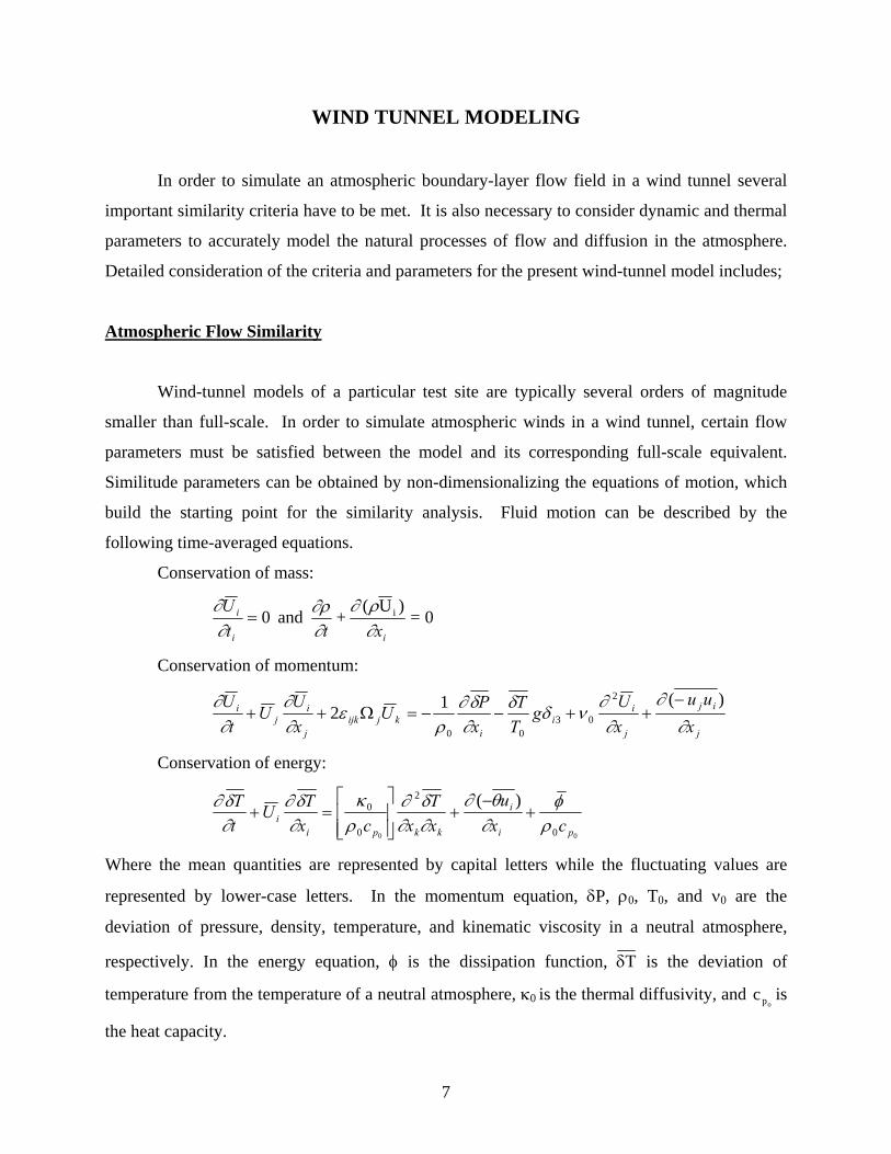
Conservation of mass:

0=)U(+ and 0 i

ii

i

xttU

∂ρ∂

∂∂ρ

∂∂

=

Conservation of momentum:

j

ij

j

ii

ikjijk

j

ij

i

xuu

xU

gTT

xPU

xU

Ut

U∂

∂∂∂

νδδ∂δ∂

ρε

∂∂

∂∂ )(12

2

0300

−++−−=Ω++

Conservation of energy:

00 0

2

0

0 )(

pi

i

kkpii cx

uxxT

cxTU

tT

ρφ

∂θ∂

∂∂δ∂

ρκ

∂δ∂

∂δ∂

+−

+⎥⎥⎦

⎤

⎢⎢⎣

⎡=+

Where the mean quantities are represented by capital letters while the fluctuating values are

represented by lower-case letters. In the momentum equation, δP, ρ0, T0, and ν0 are the

deviation of pressure, density, temperature, and kinematic viscosity in a neutral atmosphere,

respectively. In the energy equation, φ is the dissipation function, Tδ is the deviation of

temperature from the temperature of a neutral atmosphere, κ0 is the thermal diffusivity, and is

the heat capacity.

opc

7

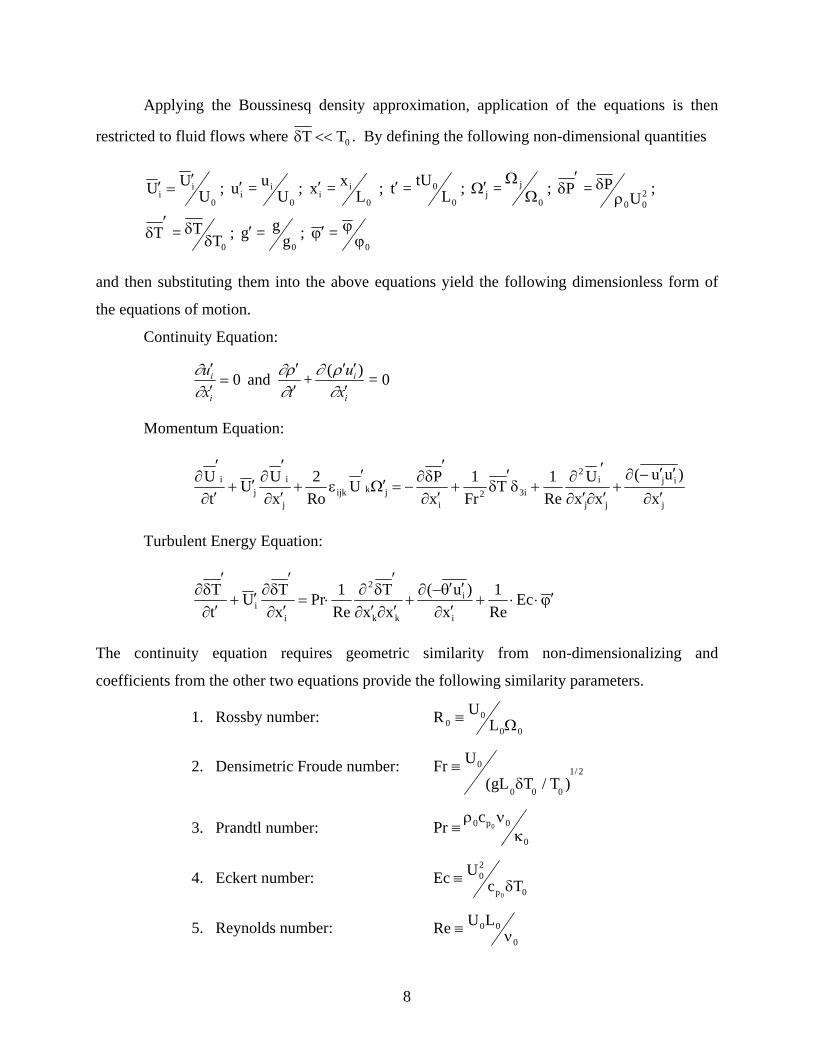
Applying the Boussinesq density approximation, application of the equations is then

restricted to fluid flows where 0TT <<δ . By defining the following non-dimensional quantities

= ; gg=g ; T

T=T

; UP=P ; = ; L

tU=t ; Lx=x ; U

u=u ; UUU

000

2000

jj

0

0

0

ii

0

ii

0

ii

ϕϕϕ′′δ

δ′δ

ρδ′

δΩΩ

Ω′′′′′=′

and then substituting them into the above equations yield the following dimensionless form of

the equations of motion.

Continuity Equation:

0=)(+ and 0i

i

i

i

xu

txu

′′′

′′

=′′

∂ρ∂

∂ρ∂

∂∂

Momentum Equation:

j

ij

jj

i2

i32i

jkijkj

ij

i

x)uu(

xxU

Re1T

Fr1

xPU

Ro2

xUU

tU

′∂

′′−∂+

′∂′∂

′∂+δ

′δ+

′∂

′δ∂

−=Ω′′

ε+′∂

′∂′+

′∂

′∂

Turbulent Energy Equation:

ϕ′⋅⋅+′∂′θ′−∂

+′∂′∂

′δ∂

⋅=′∂

′δ∂′+

′∂

′δ∂ Ec

Re1

x)u(

xxT

Re1Pr

xTU

tT

i

i

kk

2

ii

The continuity equation requires geometric similarity from non-dimensionalizing and

coefficients from the other two equations provide the following similarity parameters.

1. Rossby number: 00

00 L

UR Ω≡

2. Densimetric Froude number: )T/TgL(

UFr000

2/10

δ≡

3. Prandtl number: 0

0p0 0cPr κ

νρ≡

4. Eckert number: 0p

20

TcUEc

0δ≡

5. Reynolds number: 0

00LURe ν≡

8

In the dimensionless momentum equation, the Rossby number is extracted from the

denominator of the third term on the left side. The Rossby number represents the ratio of

advective acceleration to Coriolis acceleration due to the rotation of the earth. If the Rossby

number is large, Coriolis accelerations are small. In nature, the rotation of the earth influences

the upper layers of the atmosphere; thus, the Rossby number is small and becomes important to

match, and the corresponding term in the momentum equation is sustained. However, typical

wind tunnels are not rotating and the Rossby number is infinite, allowing the corresponding term

in the dimensionless momentum equation to approach zero. Most modelers have assumed the

Rossby number to be large, thus, neglecting the respective term in the equations of motion and

ignoring the Rossby number as a criterion for modeling. Snyder (1981) showed that the

characteristic length scale, L0, must be smaller than 5 km in order to simulate diffusion under

neutrally stable conditions in relatively flat terrain. Since the UC Davis wind tunnel produces a

boundary layer with a height of roughly one meter, the surface layer extends 20 cm above the

floor of the wind tunnel. In this region the velocity spectrum is accurately modeled. The Rossby

number can then be ignored in this region. Because the testing is limited to the lower 10% to

15% of the boundary layer, the length in longitudinal direction, which can be modeled, has to be

no more than a few kilometers.

Derived from the denominator of the second term on the right side of the dimensionless

momentum equation, the square of the Froude number represents the ratio of inertial forces to

buoyancy forces. High values of the Froude number infer that the inertial forces are dominant.

For values equal or less than unity, thermal effects become important. Since the conditions

inside the UC Davis wind tunnel are inherently isothermal, the wind tunnel generates a neutrally

stable boundary layer; hence, the Froude number is infinitely large, allowing the respective term

in the momentum equation to approach zero.

The third parameter is the Prandtl number, which is automatically matched between the

wind-tunnel flow and full-scale winds if the same fluid is used.

The Eckert number criterion is important only in compressible flow, which is not of

interest in a low-speed wind tunnel. Because the testing speed in the present study did not

exceed 11.5 ft/s, the Eckert number was negligible.

Reynolds number represents the ratio of inertial to viscous forces. The reduced scale of a

wind-tunnel model results in a Reynolds number several orders of magnitude smaller than in full

9

scale. Thus, viscous forces are more dominant in the model than in nature. No atmospheric flow

could be modeled if strict adherence to the Reynolds number criterion was required. However,

several arguments have been made to justify the use of a smaller Reynolds number in a model.

These arguments include laminar flow analogy, Reynolds number independence, and dissipation

scaling. With the absence of thermal and Coriolis effects, several test results have shown that the

scaled model flow will be dynamically similar to the full-scale case if a critical Reynolds number

is larger than a critical independence value(Snyder; 1981). The gross structure of turbulence is

similar over a wide range of Reynolds numbers. Nearly all modelers use this approach

today.[Derksen et al. (1992, 1996), Gu et al. (2007), Hitchman & Slawson (1987), Kennedy &

Fordyce (1974), and Slawson & Sullivan (1981)]

Boundary Layer Similarity

Wind-tunnel simulation of the atmospheric boundary layer, under neutrally stable

conditions, also must meet non-dimensional boundary-layer similarity parameters between the

scaled-model flow and its full-scale counterpart. The most important conditions are:

1. The normalized mean velocity, turbulent intensity, and turbulent energy profiles.

2. The roughness Reynolds number, ν= /uzRe *0z .

3. Jensen’s(1958) length-scale criterion of z0/H.

4. The ratio of H/δ for H greater than H/δ > 0.2.

In the turbulent core of a neutrally stable atmospheric boundary layer, the relationship

between the local flow velocity, U, versus its corresponding height, z, may be represented by the

following velocity-profile equation.

α

∞

⎟⎠⎞

⎜⎝⎛δ

=z

UU

U∞ is the mean velocity of the inviscid flow above the boundary layer, δ is the height of the

boundary layer, and α is the power-law exponent, which represents the upwind surface

conditions. Wind-tunnel flow can be shaped such that the exponent α will closely match its

10

corresponding full-scale value, which can be determined from field measurements of the local

winds. The required power-law exponent, α, can then be obtained by choosing the appropriate

type and distribution of roughness elements over the wind-tunnel flow-development section.

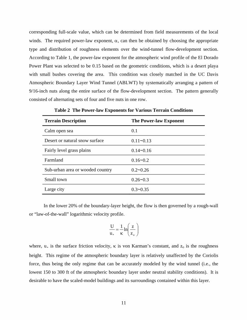
According to Table 1, the power-law exponent for the atmospheric wind profile of the El Dorado

Power Plant was selected to be 0.15 based on the geometric conditions, which is a desert playa

with small bushes covering the area. This condition was closely matched in the UC Davis

Atmospheric Boundary Layer Wind Tunnel (ABLWT) by systematically arranging a pattern of

9/16-inch nuts along the entire surface of the flow-development section. The pattern generally

consisted of alternating sets of four and five nuts in one row.

Table 2 The Power-law Exponents for Various Terrain Conditions

Terrain Description The Power-law Exponent

Calm open sea 0.1

Desert or natural snow surface 0.11∼0.13

Fairly level grass plains 0.14∼0.16

Farmland 0.16∼0.2

Sub-urban area or wooded country 0.2∼0.26

Small town 0.26∼0.3

Large city 0.3∼0.35

In the lower 20% of the boundary-layer height, the flow is then governed by a rough-wall

or “law-of-the-wall” logarithmic velocity profile.

⎟⎟⎠

⎞⎜⎜⎝

⎛κ

=o* z

zln1uU

where, is the surface friction velocity, κ is von Karman’s constant, and z*u o is the roughness

height. This regime of the atmospheric boundary layer is relatively unaffected by the Coriolis

force, thus being the only regime that can be accurately modeled by the wind tunnel (i.e., the

lowest 150 to 300 ft of the atmospheric boundary layer under neutral stability conditions). It is

desirable to have the scaled-model buildings and its surroundings contained within this layer.

11

The geometric scale of the model should be determined by the size of the wind tunnel,

the roughness height, zo, and the power-law index, α. With a boundary-layer height of 3 ft in the

test section, the surface layer would be 0.7 ft deep for the U.C. Davis ABLWT. For the present

study, this boundary layer height and the surface layer depth correspond to full-scale length of

853 ft and 171 ft, respectively. Since the highest elevation of the site investigated is about 92 ft

full-scale, the entire testing model is contained in the surface layer.

Due to scaling effects, a good simulation of the boundary-layer profiles only can be

attained in wind tunnels with long flow-development sections. For full-scale matching of the

normalized mean velocity profile, an upwind fetch of approximately 10 to 25 boundary-layer

heights is desired. To fully simulate the normalized turbulent intensity and energy spectra

profiles, the flow-development section needs to extend to about 50 and 100 to 500 times the

boundary-layer height, respectively. These profiles must at least meet full-scale similarities in

the surface-layer region. However, with the addition of spires and other flow tripping devices,

the flow development length can be reduced to less than 20 boundary layer heights for most

engineering applications. In the U.C. Davis ABLWT, the maximum values of turbulent intensity

near the surface range from 35% to 40%, similar to that in full scale. Thus, the turbulent intensity

profile, , should agree reasonably with full-scale, particularly in the region where

testing is performed.

z versusu/u′

The second boundary-layer condition involves the roughness Reynolds number, Rez.

According to the criterion given by Sutton (1949), Reynolds number independence is attained

when the roughness Reynolds number is defined as follows.

5.2zuRe 0*z ≥

ν=

u* is the friction speed, z0 is the surface roughness length, and ν is the kinematic viscosity. Rez

larger than 2.5 ensures that the flow is aerodynamically rough. Therefore, wind tunnels with a

high enough roughness Reynolds numbers are able to simulate full-scale aerodynamically rough

flows exactly. To generate a rough surface in the wind tunnel, roughness elements are placed on

the wind-tunnel floor. The height of the elements must be larger than the height of the viscous

sub-layer in order to trip the flow. The UC Davis ABLWT satisfies this condition, since the

roughness Reynolds number is about 40, when the wind-tunnel free-stream velocity, U∞, is equal

12

to 12.5 ft/s, the friction speed, , is 0.79 ft/s, and the roughness height, zu* o, is 0.1 inch. Thus, the

flow setting satisfies the Re number independence criterion and dynamically simulates the flow.

This validity sustains for various testing condition in the present study.

To simulate the pressure distribution on objects in the atmospheric wind, Jensen (1958)

found that the surface roughness to object-height ratio in the wind tunnel must be equal to that of

the atmospheric boundary layer, i.e., zo/H in the wind tunnel must match the full-scale value.

Thus, the geometric scaling should be accurately modeled.

The third boundary layer condition is the characteristic scale height to boundary layer

ratio, H/δ. There are two possible ranges for this ratio. If H/δ is larger than or equal to 0.2, then

the ratios must be matched. If (H/δ)Full Scale is smaller than 0.2, then of (H/δ)Wind Tunnel< 0.2.

Using a logarithmic profile equation, instead of the power-law velocity profile, this constrains

the physical model to 10% to 15% of the wind-tunnel boundary-layer height.

Along with these conditions, two other constraints have to be met. First, the mean stream

wise pressure gradient in the wind tunnel must be zero. Even if high- and low-pressure systems

drive atmospheric boundary-layer flows, the magnitude of the pressure gradient in the flow

direction is negligible compared to the dynamic pressure variation caused by the boundary layer.

The other constraint is that the model should not take up more than 5% to 15% of the cross-

sectional area at any downwind location. This assures that local flow acceleration affecting the

stream wise pressure gradient will not distort the simulation flow. It will be shown later in this

report that the present testing model takes less than 5% cross-sectional area.

U.C. Davis ABLWT is not capable of simulating unstable boundary layer flows. In fact,

simulation of unstable boundary layer flows could be a disadvantage due to the artificial

secondary flows generated by the heating, which dominate and distort the longitudinal mean-

flow properties, thus, invalidating the similarity criteria. However, this is not considered to be a

major constraint, since the winds that produce an annual average dispersion are sufficiently

strong, that for flow over a complex terrain, the primary source of turbulence is due to

mechanical shear and not due to diurnal heating, or cooling effects in the atmosphere.

13

Scaled Model Design and Construction

Although the main objective of the present study is to develop a general model of an

ACC system, it is necessary for comparison purposes to select an existing unit and to construct

the scaled model with the geometric conditions of that unit. Considering the accessibility of field

data and detailed geometry of the plant supplied by EPRI and the present research team, the El

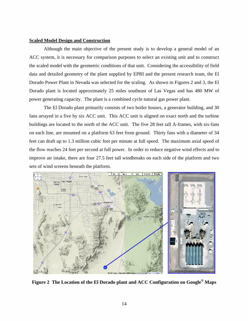
Dorado Power Plant in Nevada was selected for the scaling. As shown in Figures 2 and 3, the El

Dorado plant is located approximately 25 miles southeast of Las Vegas and has 480 MW of

power generating capacity. The plant is a combined cycle natural gas power plant.

The El Dorado plant primarily consists of two boiler houses, a generator building, and 30

fans arrayed in a five by six ACC unit. This ACC unit is aligned on exact north and the turbine

buildings are located to the north of the ACC unit. The five 28 feet tall A-frames, with six-fans

on each line, are mounted on a platform 63 feet from ground. Thirty fans with a diameter of 34

feet can draft up to 1.3 million cubic feet per minute at full speed. The maximum axial speed of

the flow reaches 24 feet per second at full power. In order to reduce negative wind effects and to

improve air intake, there are four 27.5 feet tall windbreaks on each side of the platform and two

sets of wind screens beneath the platform.

Figure 2 The Location of the El Dorado plant and ACC Configuration on Google® Maps

14

Figure 3 Side Views of the El Dorado Power Plant

Due to the limited sizes of micro fans, the fan size became the highest priority in deciding

the scale of the model. The micro fans used in the study are originally used for cooling laptop

computers and have a diameter of 4 cm (≈ 1.6 inch). The scale factors of the fans were 1 to 260

with a fan diameter of 34 feet in full scale. A series of verifications were done to check if this

scale factor meets previously presented scaling criteria.

Once the model is installed in the test section of the wind tunnel, the model shrinks the

flow area and accordingly increases the speed. The blockage effect of the model can be

estimated by the ratio of cross-sectional area of the model to the cross sectional area of the test

section. Compensating for this effect is difficult, as pointed out by Isyumov and Tanaka (1979).

Isymuov and Tanaka reported that the flow distortion is negligible with a blockage ratio less than

5%. Therefore, the scaled model cross-sectional area has to be less than 5% of the cross

sectional area of the test section to meet the Isyumov criterion. Considering the cross-sectional

area of the UC Davis wind tunnel (3.9 ft by 5.2 ft) and the area of the ACC unit of the El Dorado

plant (233 ft by 28 ft), any scale ratio larger than 79 meets the Isyumov criterion. The model of

ACC with a scale factor of 260 will provide a blockage ratio of approximately 0.5%.

The typical atmospheric boundary layer thickness is known to be 1,200 ft over suburban

terrain, 900 ft over open area, and 700 ft over ocean. The ratio of atmospheric boundary layer

15

thickness to the thickness of the simulated boundary layer represents another scale factor.

Considering the test section height of the U.C. Davis ABLWT (5.5 ft) and the possible

disturbance at the top of the boundary layer, caused by the traversing mechanism, a scale factor

between 220 and 270 should be applied to simulate the atmospheric boundary layer over desert

terrains. The scale factor of 260 also meets this condition.

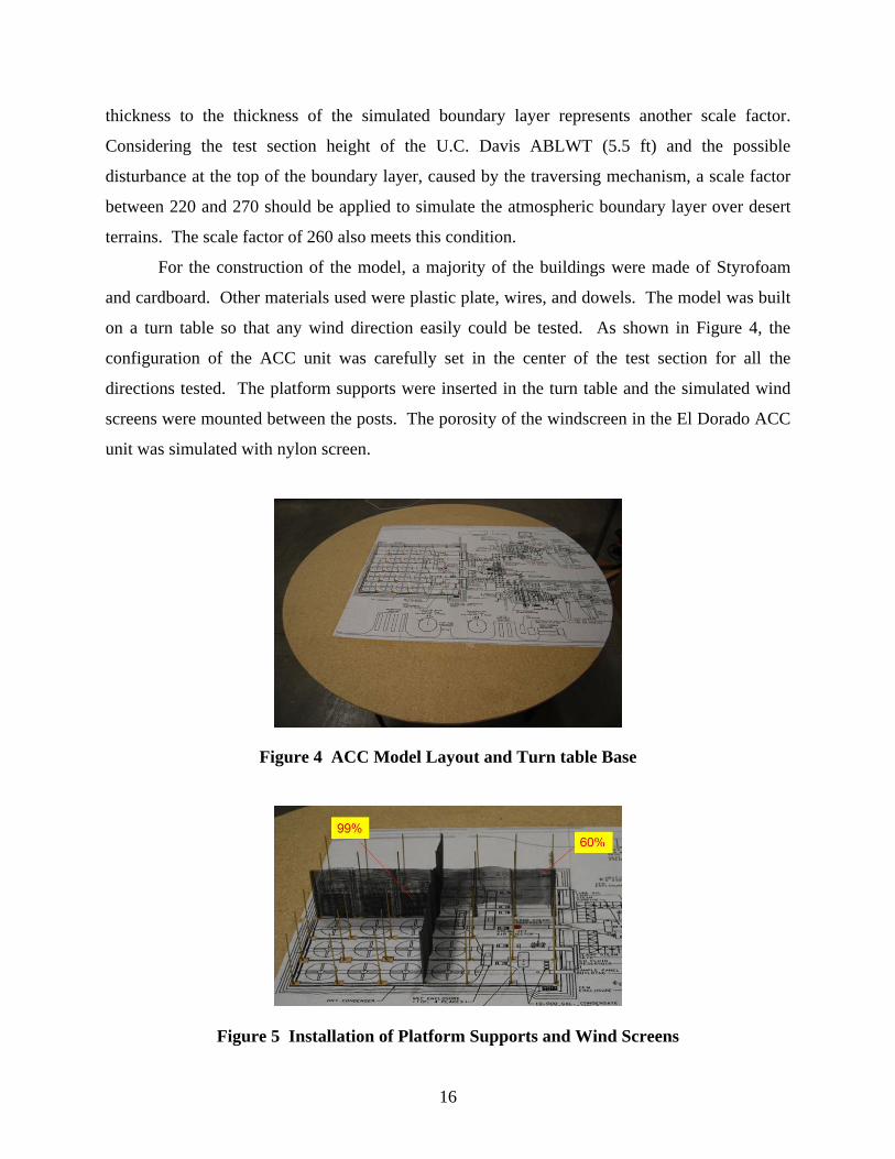
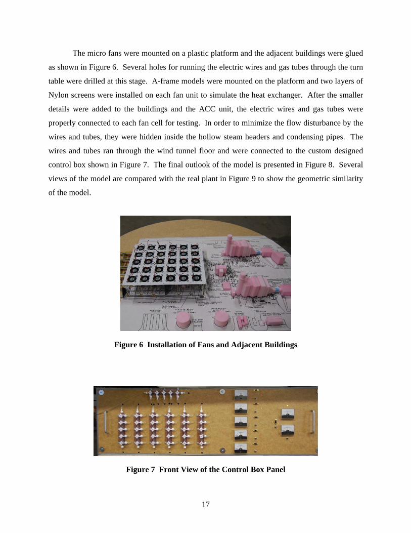
For the construction of the model, a majority of the buildings were made of Styrofoam

and cardboard. Other materials used were plastic plate, wires, and dowels. The model was built

on a turn table so that any wind direction easily could be tested. As shown in Figure 4, the

configuration of the ACC unit was carefully set in the center of the test section for all the

directions tested. The platform supports were inserted in the turn table and the simulated wind

screens were mounted between the posts. The porosity of the windscreen in the El Dorado ACC

unit was simulated with nylon screen.

Figure 4 ACC Model Layout and Turn table Base

Figure 5 Installation of Platform Supports and Wind Screens

16

The micro fans were mounted on a plastic platform and the adjacent buildings were glued

as shown in Figure 6. Several holes for running the electric wires and gas tubes through the turn

table were drilled at this stage. A-frame models were mounted on the platform and two layers of

Nylon screens were installed on each fan unit to simulate the heat exchanger. After the smaller

details were added to the buildings and the ACC unit, the electric wires and gas tubes were

properly connected to each fan cell for testing. In order to minimize the flow disturbance by the

wires and tubes, they were hidden inside the hollow steam headers and condensing pipes. The

wires and tubes ran through the wind tunnel floor and were connected to the custom designed

control box shown in Figure 7. The final outlook of the model is presented in Figure 8. Several

views of the model are compared with the real plant in Figure 9 to show the geometric similarity

of the model.

Figure 6 Installation of Fans and Adjacent Buildings

Figure 7 Front View of the Control Box Panel

17

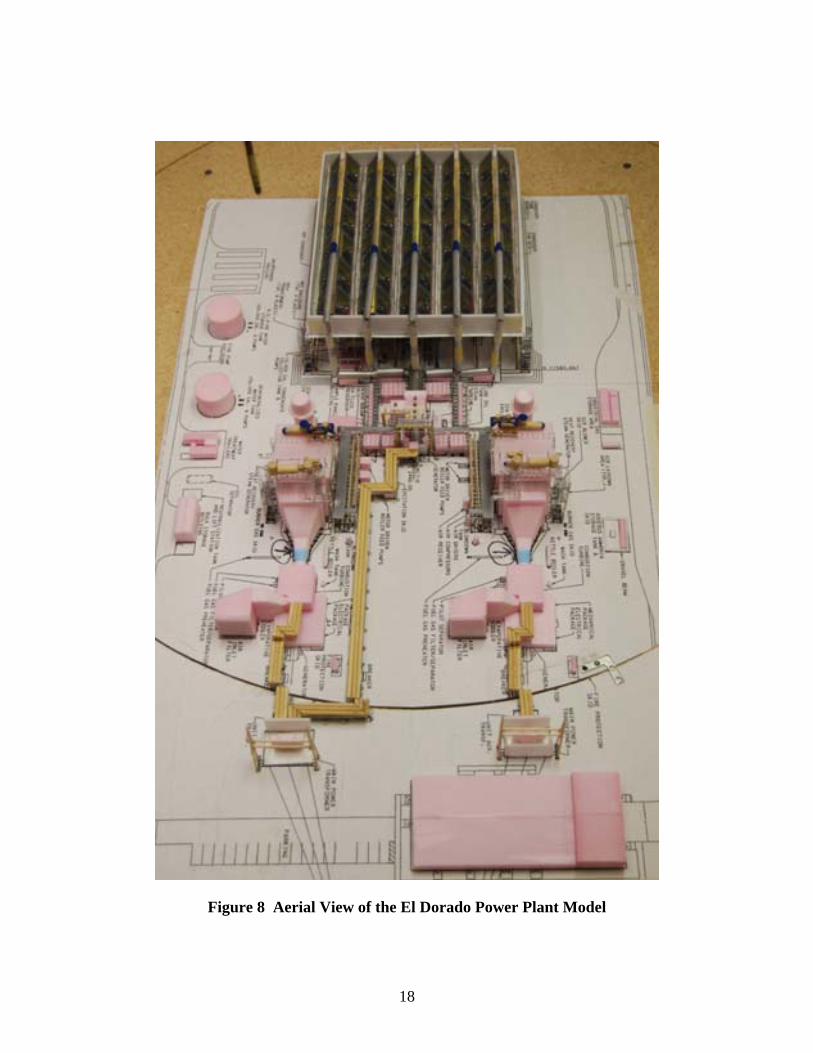
Figure 8 Aerial View of the El Dorado Power Plant Model

18

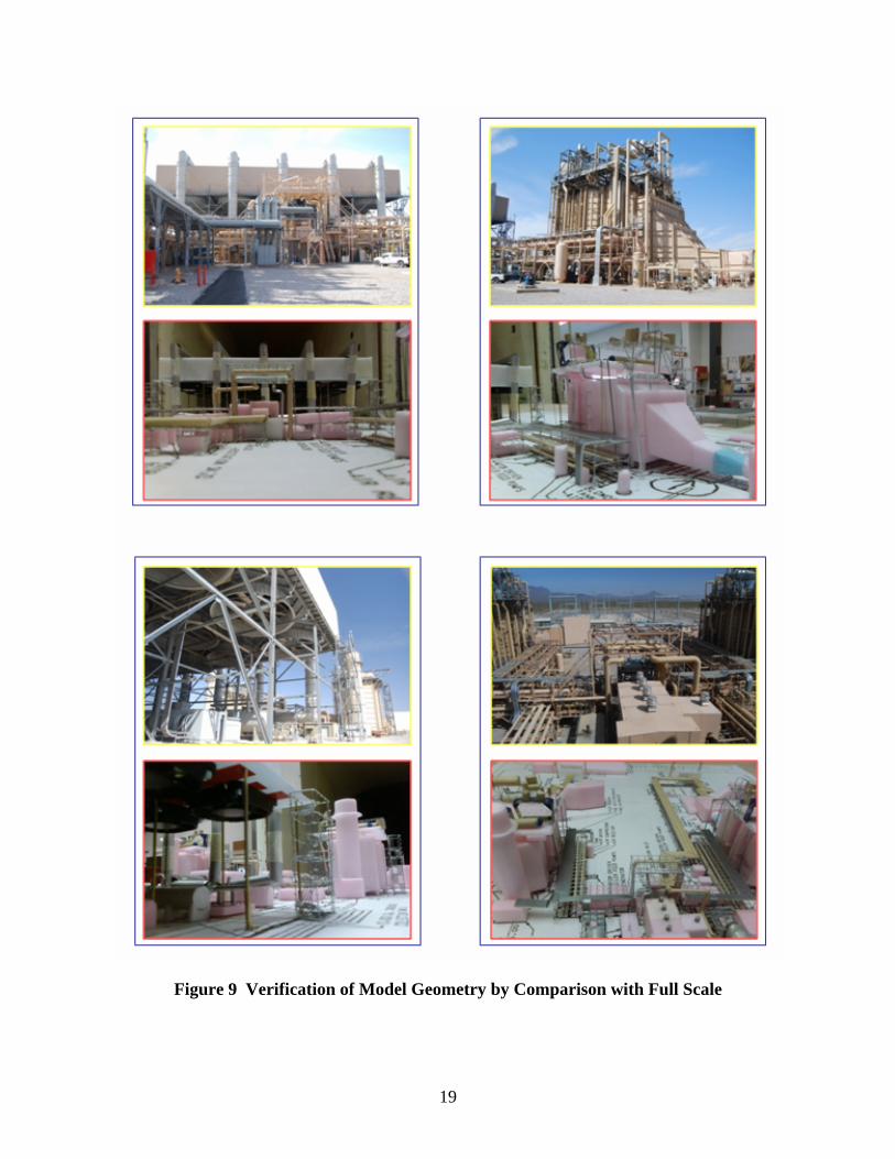
Figure 9 Verification of Model Geometry by Comparison with Full Scale

19

TESTING FACILITIES

The Atmospheric Boundary Layer Wind Tunnel at UC Davis

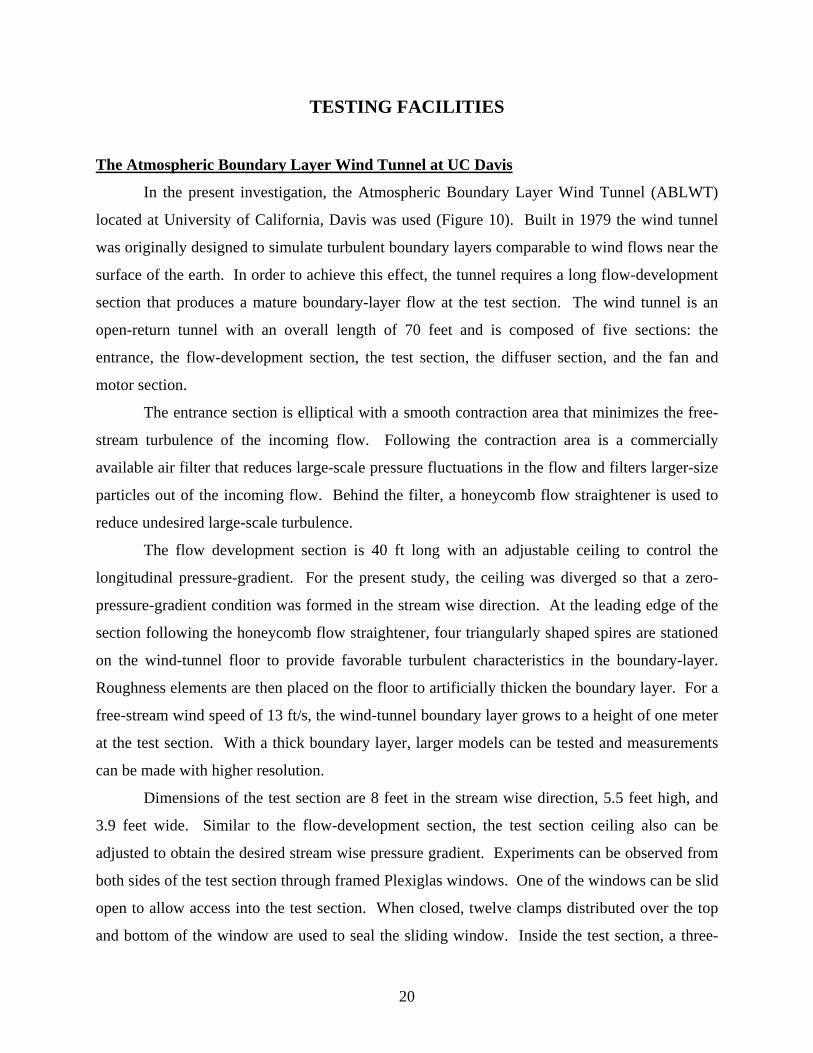
In the present investigation, the Atmospheric Boundary Layer Wind Tunnel (ABLWT)

located at University of California, Davis was used (Figure 10). Built in 1979 the wind tunnel

was originally designed to simulate turbulent boundary layers comparable to wind flows near the

surface of the earth. In order to achieve this effect, the tunnel requires a long flow-development

section that produces a mature boundary-layer flow at the test section. The wind tunnel is an

open-return tunnel with an overall length of 70 feet and is composed of five sections: the

entrance, the flow-development section, the test section, the diffuser section, and the fan and

motor section.

The entrance section is elliptical with a smooth contraction area that minimizes the free-

stream turbulence of the incoming flow. Following the contraction area is a commercially

available air filter that reduces large-scale pressure fluctuations in the flow and filters larger-size

particles out of the incoming flow. Behind the filter, a honeycomb flow straightener is used to

reduce undesired large-scale turbulence.

The flow development section is 40 ft long with an adjustable ceiling to control the

longitudinal pressure-gradient. For the present study, the ceiling was diverged so that a zero-

pressure-gradient condition was formed in the stream wise direction. At the leading edge of the

section following the honeycomb flow straightener, four triangularly shaped spires are stationed

on the wind-tunnel floor to provide favorable turbulent characteristics in the boundary-layer.

Roughness elements are then placed on the floor to artificially thicken the boundary layer. For a

free-stream wind speed of 13 ft/s, the wind-tunnel boundary layer grows to a height of one meter

at the test section. With a thick boundary layer, larger models can be tested and measurements

can be made with higher resolution.

Dimensions of the test section are 8 feet in the stream wise direction, 5.5 feet high, and

3.9 feet wide. Similar to the flow-development section, the test section ceiling also can be

adjusted to obtain the desired stream wise pressure gradient. Experiments can be observed from

both sides of the test section through framed Plexiglas windows. One of the windows can be slid

open to allow access into the test section. When closed, twelve clamps distributed over the top

and bottom of the window are used to seal the sliding window. Inside the test section, a three-

20

dimensional probe-positioning system is installed in the ceiling to provide fast and accurate

sensor placement. The traversing scissors, which provide vertical motion to the probe, are made

of aerodynamically shaped struts to minimize flow disturbances.

The diffuser section is 7.8 ft long and has an expansion area that provides a continuous

transition from the rectangular cross-section of the test section to the circular cross-sectional area

of the fan. To eliminate upstream swirl effects from the fan and avoid flow separation in the

diffuser section, fiberboard and honeycomb flow straightener are placed between the fan and the

diffuser section.

The fan consists of eight constant-pitch blades, 6 feet in diameter, and is powered by a 56

kW (75 hp) variable-speed DC motor. A dual belt and pulley drive system is used to couple the

motor and the fan.

Figure 10 Schematic Diagram of the UC Davis Atmospheric BoundaTunnel

21

75

ry Layer Wind

Instrumentation and Measurement System

Wind-tunnel measurements of the mean velocity and turbulent characteristics were

performed using hot-wire anemometry. A Thermo Systems Inc. (TSI) single hot-wire sensor

model 1210-60 was used to measure the wind quantities. The sensor was installed at the end of a

TSI 1150 50-cm probe support, which was secured to the support plate of the three-dimensional

sensor positioning system in the U.C. Davis ABLWT test section. A 50-ft shielded tri-axial

cable was used to connect the probe support and sensor arrangement to a TSI IFA 100 constant

temperature anemometry unit with signal conditioners.

Hot-wire sensors were calibrated in the ABLWT test section over a range of velocities in

the wind-tunnel boundary layer. Signal-conditioned voltage readings of the hot-wire sensor were

then matched against the velocity measurements from a pitot-static tube connected to a Meriam

34FB2 oil micro-manometer, which has a resolution of 1/1,000 inch of oil. The specific gravity

of the oil in the oil micro-manometer was 0.934. The pitot-static tube was secured to an

aerodynamically shaped stand and was positioned so that its flow-sensing tip is normal to the

flow and situated near the volumetric center of the test section. Normal to the flow, the end of

the hot-wire sensor was then traversed to a position 4 inch next to the tip of the Pitot-static tube.

Using a LabVIEW data acquisition system, all the data was acquired and digitally

recorded for each point at a sampling rate of 1000 Hz for 30 seconds, which is equivalent to one

hour of field measurement with 20 MPH wind speeds at a height of 520 ft. This yielded 30,000

voltage readings from the anemometer transducer that were individually converted to

instantaneous wind speeds by applying a calibration curve, which was acquired prior to the

testing. The 30,000 samples were then statistically analyzed to produce a single average wind

speed and the standard deviation (turbulent intensity). The resulting mean speeds and turbulent

intensities represent one-hour of full-scale measurements of time averaged wind speeds and

fluctuations.

In order to measure the recirculation rate of exhausted gas, concentrations of an ethane

tracer gas were measured with the use of a Rosemount Analytical 400A hydrocarbon analyzer.

This instrument uses flame-ionization detection to determine trace concentrations of

hydrocarbons in the air. The ethane-air samples are iso-kinetically aspirated into a burner where

the sample is burned with a mixture of medical-rated air (40% hydrogen and 60% nitrogen).

22

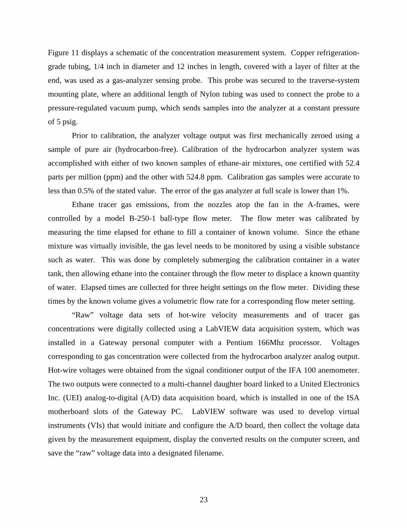
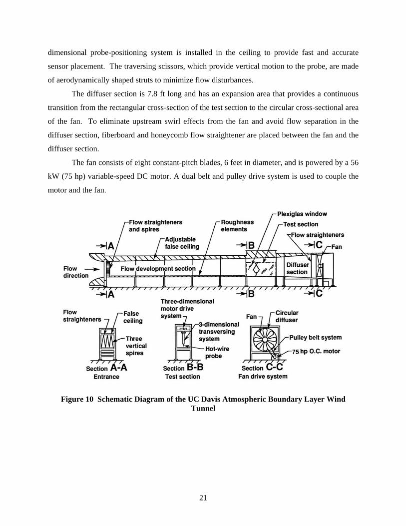
Figure 11 displays a schematic of the concentration measurement system. Copper refrigeration-

grade tubing, 1/4 inch in diameter and 12 inches in length, covered with a layer of filter at the

end, was used as a gas-analyzer sensing probe. This probe was secured to the traverse-system

mounting plate, where an additional length of Nylon tubing was used to connect the probe to a

pressure-regulated vacuum pump, which sends samples into the analyzer at a constant pressure

of 5 psig.

Prior to calibration, the analyzer voltage output was first mechanically zeroed using a

sample of pure air (hydrocarbon-free). Calibration of the hydrocarbon analyzer system was

accomplished with either of two known samples of ethane-air mixtures, one certified with 52.4

parts per million (ppm) and the other with 524.8 ppm. Calibration gas samples were accurate to

less than 0.5% of the stated value. The error of the gas analyzer at full scale is lower than 1%.

Ethane tracer gas emissions, from the nozzles atop the fan in the A-frames, were

controlled by a model B-250-1 ball-type flow meter. The flow meter was calibrated by

measuring the time elapsed for ethane to fill a container of known volume. Since the ethane

mixture was virtually invisible, the gas level needs to be monitored by using a visible substance

such as water. This was done by completely submerging the calibration container in a water

tank, then allowing ethane into the container through the flow meter to displace a known quantity

of water. Elapsed times are collected for three height settings on the flow meter. Dividing these

times by the known volume gives a volumetric flow rate for a corresponding flow meter setting.

“Raw” voltage data sets of hot-wire velocity measurements and of tracer gas

concentrations were digitally collected using a LabVIEW data acquisition system, which was

installed in a Gateway personal computer with a Pentium 166Mhz processor. Voltages

corresponding to gas concentration were collected from the hydrocarbon analyzer analog output.

Hot-wire voltages were obtained from the signal conditioner output of the IFA 100 anemometer.

The two outputs were connected to a multi-channel daughter board linked to a United Electronics

Inc. (UEI) analog-to-digital (A/D) data acquisition board, which is installed in one of the ISA

motherboard slots of the Gateway PC. LabVIEW software was used to develop virtual

instruments (VIs) that would initiate and configure the A/D board, then collect the voltage data

given by the measurement equipment, display the converted results on the computer screen, and

save the “raw” voltage data into a designated filename.

23

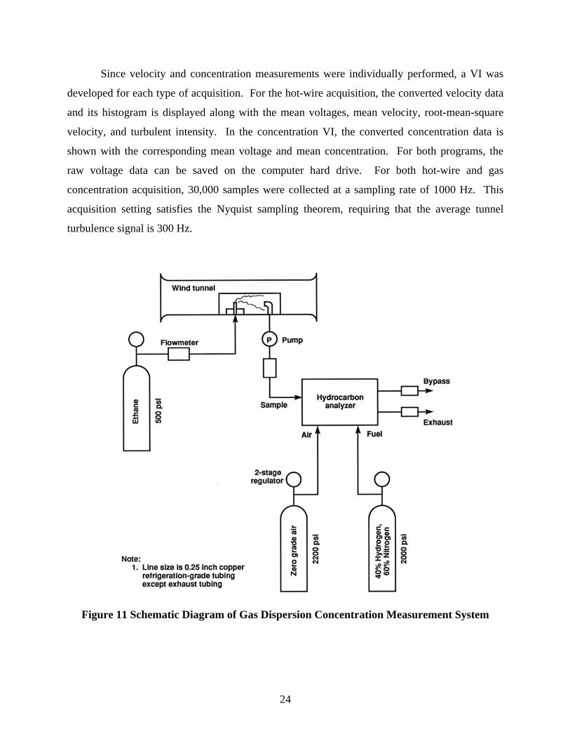
Since velocity and concentration measurements were individually performed, a VI was

developed for each type of acquisition. For the hot-wire acquisition, the converted velocity data

and its histogram is displayed along with the mean voltages, mean velocity, root-mean-square

velocity, and turbulent intensity. In the concentration VI, the converted concentration data is

shown with the corresponding mean voltage and mean concentration. For both programs, the

raw voltage data can be saved on the computer hard drive. For both hot-wire and gas

concentration acquisition, 30,000 samples were collected at a sampling rate of 1000 Hz. This

acquisition setting satisfies the Nyquist sampling theorem, requiring that the average tunnel

turbulence signal is 300 Hz.

Figure 11 Schematic Diagram of Gas Dispersion Concentration Measurement System

24

TESTING METHODOLOGY

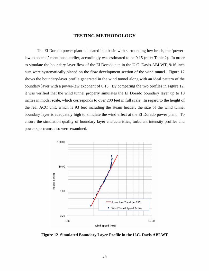
The El Dorado power plant is located in a basin with surrounding low brush, the ‘power-

law exponent,’ mentioned earlier, accordingly was estimated to be 0.15 (refer Table 2). In order

to simulate the boundary layer flow of the El Dorado site in the U.C. Davis ABLWT, 9/16 inch

nuts were systematically placed on the flow development section of the wind tunnel. Figure 12

shows the boundary-layer profile generated in the wind tunnel along with an ideal pattern of the

boundary layer with a power-law exponent of 0.15. By comparing the two profiles in Figure 12,

it was verified that the wind tunnel properly simulates the El Dorado boundary layer up to 10

inches in model scale, which corresponds to over 200 feet in full scale. In regard to the height of

the real ACC unit, which is 93 feet including the steam header, the size of the wind tunnel

boundary layer is adequately high to simulate the wind effect at the El Dorado power plant. To

ensure the simulation quality of boundary layer characteristics, turbulent intensity profiles and

power spectrums also were examined.

Figure 12 Simulated Boundary Layer Profile in the U.C. Davis ABLWT

25

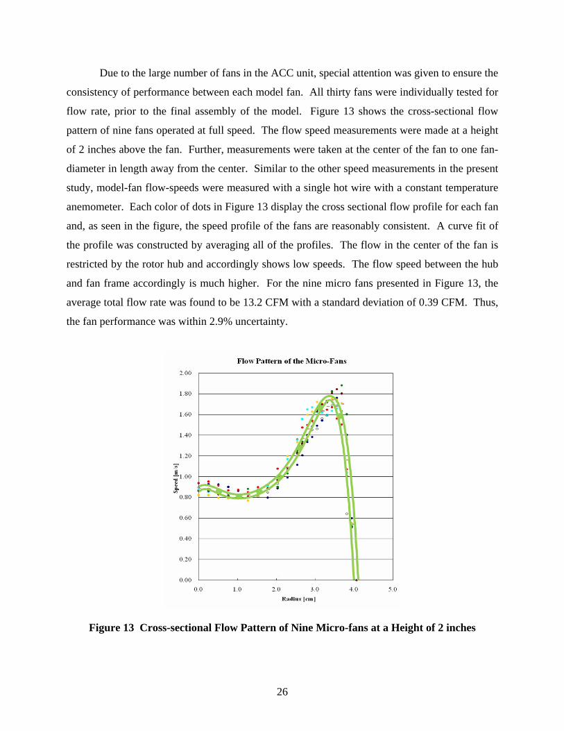
Due to the large number of fans in the ACC unit, special attention was given to ensure the

consistency of performance between each model fan. All thirty fans were individually tested for

flow rate, prior to the final assembly of the model. Figure 13 shows the cross-sectional flow

pattern of nine fans operated at full speed. The flow speed measurements were made at a height

of 2 inches above the fan. Further, measurements were taken at the center of the fan to one fan-

diameter in length away from the center. Similar to the other speed measurements in the present

study, model-fan flow-speeds were measured with a single hot wire with a constant temperature

anemometer. Each color of dots in Figure 13 display the cross sectional flow profile for each fan

and, as seen in the figure, the speed profile of the fans are reasonably consistent. A curve fit of

the profile was constructed by averaging all of the profiles. The flow in the center of the fan is

restricted by the rotor hub and accordingly shows low speeds. The flow speed between the hub

and fan frame accordingly is much higher. For the nine micro fans presented in Figure 13, the

average total flow rate was found to be 13.2 CFM with a standard deviation of 0.39 CFM. Thus,

the fan performance was within 2.9% uncertainty.

Figure 13 Cross-sectional Flow Pattern of Nine Micro-fans at a Height of 2 inches

26

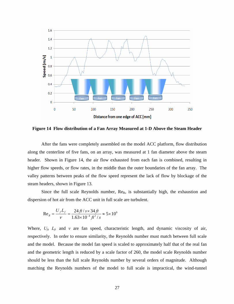
Figure 14 Flow distribution of a Fan Array Measured at 1-D Above the Steam Header

After the fans were completely assembled on the model ACC platform, flow distribution

along the centerline of five fans, on an array, was measured at 1 fan diameter above the steam

header. Shown in Figure 14, the air flow exhausted from each fan is combined, resulting in

higher flow speeds, or flow rates, in the middle than the outer boundaries of the fan array. The

valley patterns between peaks of the flow speed represent the lack of flow by blockage of the

steam headers, shown in Figure 13.

Since the full scale Reynolds number, ReR, is substantially high, the exhaustion and

dispersion of hot air from the ACC unit in full scale are turbulent.

624 105

/1063.134/24Re ×≈

××

== − sftftsftLU ff

R ν

Where, Uf, Lf, and ν are fan speed, characteristic length, and dynamic viscosity of air,

respectively. In order to ensure similarity, the Reynolds number must match between full scale

and the model. Because the model fan speed is scaled to approximately half that of the real fan

and the geometric length is reduced by a scale factor of 260, the model scale Reynolds number

should be less than the full scale Reynolds number by several orders of magnitude. Although

matching the Reynolds numbers of the model to full scale is impractical, the wind-tunnel

27

simulation is still considered to be adequate if the exhaust flow from the model is turbulent

(Snyder, 1981). This condition is generally achieved (for neutral stability conditions) for model

Reynolds number, ReM, greater than:

2300/1063.1

57.1Re 24 >××

== − sftinchUDU MMM

M ν

Due to this constraint, the model fan speed has to exceed 2.9 ft/s (≈0.8 m/s). It will be shown in

the following chapter that the Reynolds number in the present study is between 15,000 and

40,000 depending on the wind speed setting and meets this Reynolds number criterion.

Besides the Reynolds number, the ratio of exhaust air speed, ue, to the upstream wind

speed, U, has to be maintained correctly for adequate simulation [Isyumov and Tanaka (1980)].

m

e

R

e

Uu

Uu

⎟⎠⎞

⎜⎝⎛=⎟

⎠⎞

⎜⎝⎛

Where, R and m represent real scale and model scale, respectively. At the real power plant, the

upstream speed is uncontrollable and only the fan speed can be adjusted upon the level of back

pressure in steam line. For the full-scale speed ratio the fan air speed was assumed to be the total

air flow without any displacement caused by back pressure from the heat exchanger tubes and

fins. Although the fan is set to one of only three speeds (zero, half, or full speed), the continuous

variation of natural wind speeds yield an indefinite number of the speed ratio cases in full scale.

In order to estimate the upstream wind effect on the ACC unit, the meteorological data at the site

was analyzed and divided into five categories that evenly spread the statistical occurrence of

wind speeds. Table 3 shows the upstream wind speed categories and the combinations of model

fan speed and wind-tunnel speed used to meet the wind-speed ratios of the full-scale plant. In

order to properly control the model fan speed, a calibration between the fan speed and power

input was done prior to testing. The wind-tunnel speed also was calibrated to the power

frequency settings. In order to accurately model the fan air speed, the flow rate of tracer gas

issued atop the fan was taken into account. The (ue)m values in Table 3 represent the total

exhaust flow speed. The proper upstream wind speed and exhaust speed were then achieved by

controlling the respective power settings.

28

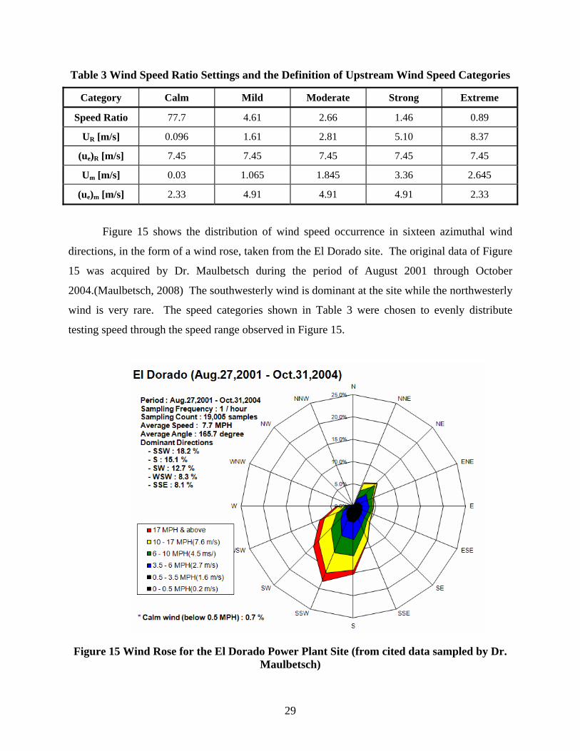
Table 3 Wind Speed Ratio Settings and the Definition of Upstream Wind Speed Categories

Category Calm Mild Moderate Strong Extreme

Speed Ratio 77.7 4.61 2.66 1.46 0.89

UR [m/s] 0.096 1.61 2.81 5.10 8.37

(ue)R [m/s] 7.45 7.45 7.45 7.45 7.45

Um [m/s] 0.03 1.065 1.845 3.36 2.645

(ue)m [m/s] 2.33 4.91 4.91 4.91 2.33

Figure 15 shows the distribution of wind speed occurrence in sixteen azimuthal wind

directions, in the form of a wind rose, taken from the El Dorado site. The original data of Figure

15 was acquired by Dr. Maulbetsch during the period of August 2001 through October

2004.(Maulbetsch, 2008) The southwesterly wind is dominant at the site while the northwesterly

wind is very rare. The speed categories shown in Table 3 were chosen to evenly distribute

testing speed through the speed range observed in Figure 15.

Figure 15 Wind Rose for the El Dorado Power Plant Site (from cited data sampled by Dr. Maulbetsch)

29

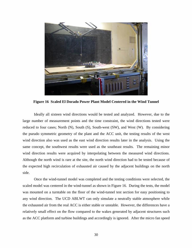
Figure 16 Scaled El Dorado Power Plant Model Centered in the Wind Tunnel

Ideally all sixteen wind directions would be tested and analyzed. However, due to the

large number of measurement points and the time constraint, the wind directions tested were

reduced to four cases; North (N), South (S), South-west (SW), and West (W). By considering

the pseudo symmetric geometry of the plant and the ACC unit, the testing results of the west

wind direction also was used as the east wind direction results later in the analysis. Using the

same concept, the southwest results were used as the southeast results. The remaining minor

wind direction results were acquired by interpolating between the measured wind directions.

Although the north wind is rare at the site, the north wind direction had to be tested because of

the expected high recirculation of exhausted air caused by the adjacent buildings on the north

side.

Once the wind-tunnel model was completed and the testing conditions were selected, the

scaled model was centered in the wind-tunnel as shown in Figure 16. During the tests, the model

was mounted on a turntable on the floor of the wind-tunnel test section for easy positioning to

any wind direction. The UCD ABLWT can only simulate a neutrally stable atmosphere while

the exhausted air from the real ACC is either stable or unstable. However, the differences have a

relatively small effect on the flow compared to the wakes generated by adjacent structures such

as the ACC platform and turbine buildings and accordingly is ignored. After the micro fan speed

30

and wind-tunnel speed were set to the values given in Table 3 and the model is set to the desired

wind direction, wind speeds were measured using hot-wire anemometry. The winds effect on the

efficiency of an ACC system is due to its effect on the rate of air indigested into the fans, the

exhaust air dispersion, and the recirculation of hot exhausted air. The recirculation due to wind

effects plays a critical role in the negative effects of the wind on ACC efficiency as Gu et al.

(2007) pointed out. The present study focused on the wind’s effect on the recirculation.

Although the relationship between the recirculation level and the efficiency of ACC is not

completely understood, it is obvious that under a specific wind direction and speed, ambient

temperature, and fan-flow rate, the ACC efficiency must be inversely proportion to the

recirculation level. Because of this, the relationship between the recirculation level and the

efficiency of the ACC system was not taken into account in the study, but the recirculation level

itself was presented throughout the report to quantitatively understand the wind’s effect.

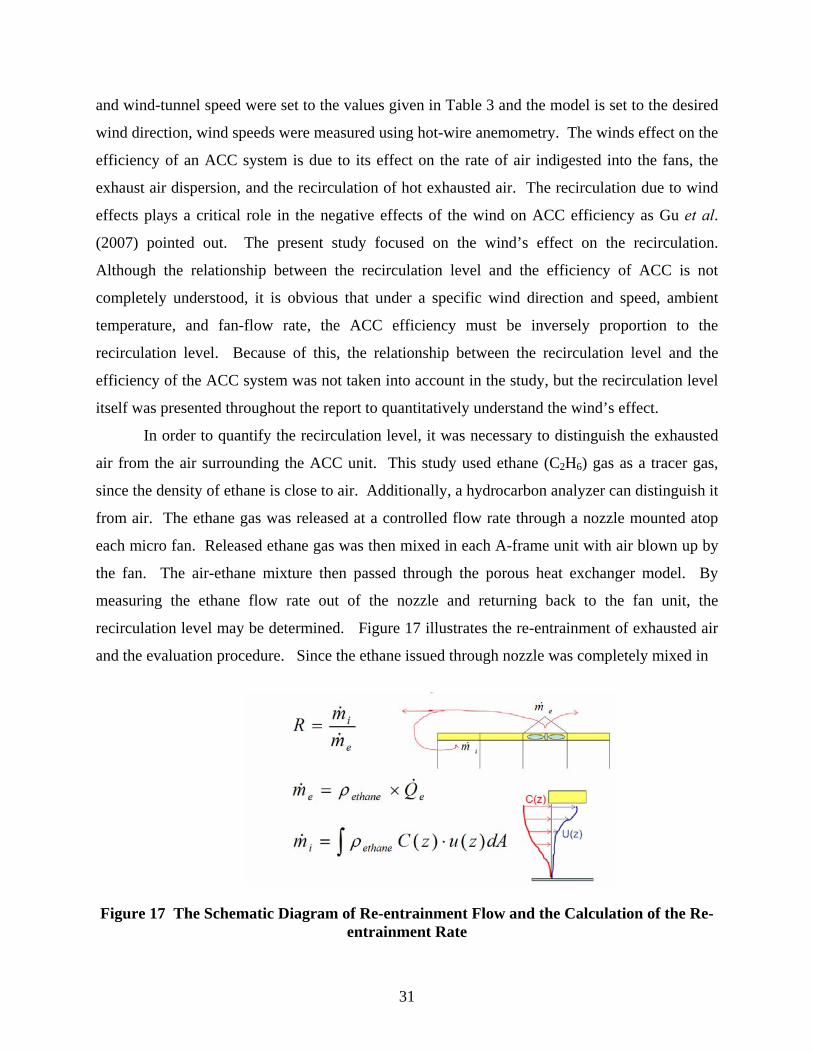
In order to quantify the recirculation level, it was necessary to distinguish the exhausted

air from the air surrounding the ACC unit. This study used ethane (C2H6) gas as a tracer gas,

since the density of ethane is close to air. Additionally, a hydrocarbon analyzer can distinguish it

from air. The ethane gas was released at a controlled flow rate through a nozzle mounted atop

each micro fan. Released ethane gas was then mixed in each A-frame unit with air blown up by

the fan. The air-ethane mixture then passed through the porous heat exchanger model. By

measuring the ethane flow rate out of the nozzle and returning back to the fan unit, the

recirculation level may be determined. Figure 17 illustrates the re-entrainment of exhausted air

and the evaluation procedure. Since the ethane issued through nozzle was completely mixed in

Figure 17 The Schematic Diagram of Re-entrainment Flow and the Calculation of the Re-entrainment Rate

31

the A-frame and exhausted through several layers of screen, the ethane exhaust rate, Qe, was

assumed to be uniform. The exhaust rate can be monitored by the flow meter at the gas

distributor and the mass flow rate of ethane exhaust can be calculated. Re-entrainment flow,

however, is not uniform in speed or concentration at the entrance plane and accordingly is more

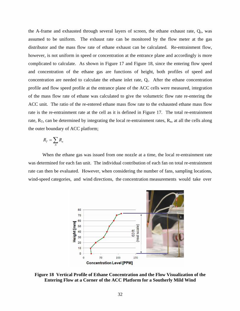
complicated to calculate. As shown in Figure 17 and Figure 18, since the entering flow speed

and concentration of the ethane gas are functions of height, both profiles of speed and

concentration are needed to calculate the ethane inlet rate, Qi. After the ethane concentration

profile and flow speed profile at the entrance plane of the ACC cells were measured, integration

of the mass flow rate of ethane was calculated to give the volumetric flow rate re-entering the

ACC unit. The ratio of the re-entered ethane mass flow rate to the exhausted ethane mass flow

rate is the re-entrainment rate at the cell as it is defined in Figure 17. The total re-entrainment

rate, RT, can be determined by integrating the local re-entrainment rates, Rn, at all the cells along

the outer boundary of ACC platform;

∑=N

nT RR

When the ethane gas was issued from one nozzle at a time, the local re-entrainment rate

was determined for each fan unit. The individual contribution of each fan on total re-entrainment

rate can then be evaluated. However, when considering the number of fans, sampling locations,

wind-speed categories, and wind directions, the concentration measurements would take over

Figure 18 Vertical Profile of Ethane Concentration and the Flow Visualization of the Entering Flow at a Corner of the ACC Platform for a Southerly Mild Wind

32

500 hours. Due to the time constraint, for most of the testing cases all the nozzles were

controlled to issue the same rate of ethane gas simultaneously and accordingly the local re-

entrainment rate values represent the total contribution of all the fan units. The individual

contribution of each fan was only examined for the worst case.

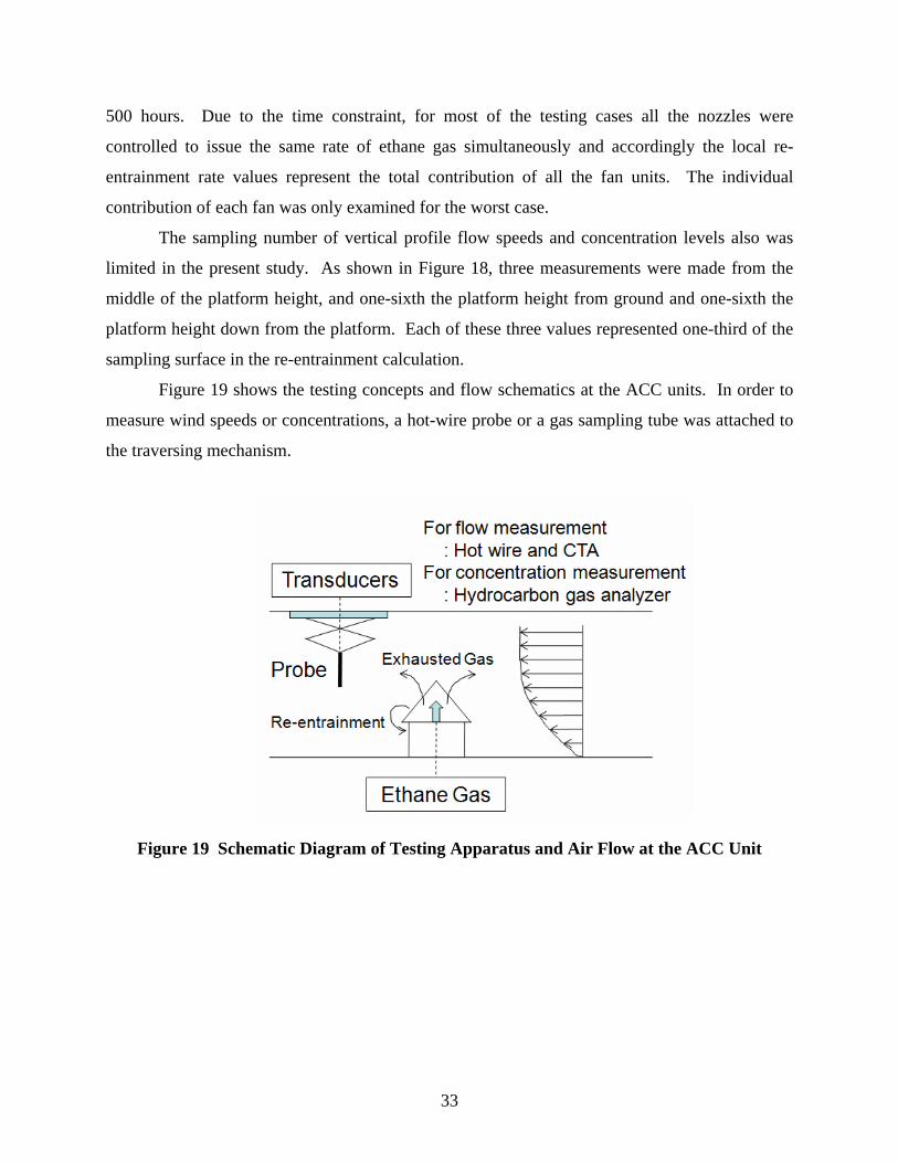
The sampling number of vertical profile flow speeds and concentration levels also was

limited in the present study. As shown in Figure 18, three measurements were made from the

middle of the platform height, and one-sixth the platform height from ground and one-sixth the

platform height down from the platform. Each of these three values represented one-third of the

sampling surface in the re-entrainment calculation.

Figure 19 shows the testing concepts and flow schematics at the ACC units. In order to

measure wind speeds or concentrations, a hot-wire probe or a gas sampling tube was attached to

the traversing mechanism.

Figure 19 Schematic Diagram of Testing Apparatus and Air Flow at the ACC Unit

33

SINGLE UNIT MODEL ANALYSIS

Wind-tunnel Testing Results

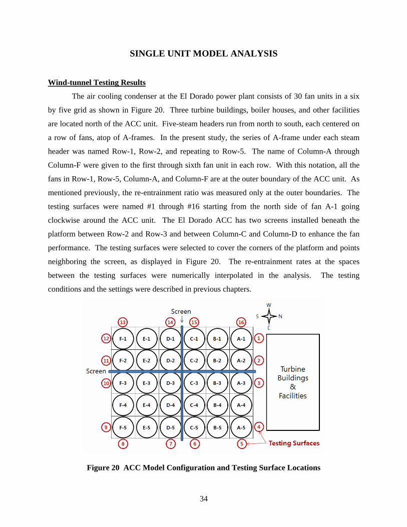
The air cooling condenser at the El Dorado power plant consists of 30 fan units in a six

by five grid as shown in Figure 20. Three turbine buildings, boiler houses, and other facilities

are located north of the ACC unit. Five-steam headers run from north to south, each centered on

a row of fans, atop of A-frames. In the present study, the series of A-frame under each steam

header was named Row-1, Row-2, and repeating to Row-5. The name of Column-A through

Column-F were given to the first through sixth fan unit in each row. With this notation, all the

fans in Row-1, Row-5, Column-A, and Column-F are at the outer boundary of the ACC unit. As

mentioned previously, the re-entrainment ratio was measured only at the outer boundaries. The

testing surfaces were named #1 through #16 starting from the north side of fan A-1 going

clockwise around the ACC unit. The El Dorado ACC has two screens installed beneath the

platform between Row-2 and Row-3 and between Column-C and Column-D to enhance the fan

performance. The testing surfaces were selected to cover the corners of the platform and points

neighboring the screen, as displayed in Figure 20. The re-entrainment rates at the spaces

between the testing surfaces were numerically interpolated in the analysis. The testing

conditions and the settings were described in previous chapters.

Figure 20 ACC Model Configuration and Testing Surface Locations

34

35

Figure 21 shows a sample of the worksheet used to calculate the re-entrainment rate and

to display the results. The first row indicates the wind speed category, defined in Table 2, the

direction of the setting, and the purity of ethane gas. In the data table, the first column lists the

testing surface numbers and the next three columns provide geometric information of the testing

surfaces. The next six columns show three sets of concentration and flow speed readings. T, M,

and B stand for Top-section, Middle-section, and Bottom-section, indicating the sampling

heights. The next three sets of data indicate the ethane flux re-entering through each section of

the testing surface. The ratio of the re-entering flux to the exhausted flux yields the re-

entrainment rate, shown in the next three columns. The last column in the table indicates the

total re-entrainment rate of each testing surface. By summing the local re-entrainment rates from

all the testing surfaces, the total re-entrainment rate may be evaluated and is shown at the bottom

of the table. Relatively high values, among the re-entrainment rate values in the table, were

highlighted. Vertical distributions of re-entrainment rates measured from the top, middle, and

bottom section of each testing surface are displayed in the lower left corner. The lower right

corner shows estimated contours of re-entrainment rates for all the fan units. In between, re-

entrainment rates are plotted along the outer boundary of the ACC unit. A total of twenty

worksheets, like Figure 21, were made from five wind speeds and four wind directions.

Appendix-A contains the twenty worksheets.

Figure 22 compares the trends of re-entrainment rate distributions for different speed and

direction settings. Each column in Figure 22 represents a wind speed setting while the rows

show the wind direction setting. Figure 22 indicates that the re-entrainment of the ACC unit is

greatly affected by both wind speed and direction, along with the interference of adjacent

buildings and the ACC. For the calm wind speed, most of the re-entrainment occurred at the

opposite side from the incoming wind. This trend indicates that the platform generates a wake

by distorting the wind and that the exhausted “hot" air and wake was drawn by the fans on the

backside of the platform. This trend was sustained for all the wind directions. The effect of the

wind and the adjacent buildings on the flow was not strong enough to stretch the wake away

from the platform.

Wind Strength Wind Direction Ethan Purity

1.3009

1.8419

2.2646

0.8667

1.4481

1.3055

Moderate N 98.5X Y width

[cm] [cm] [cm] T M B T M B T M B T M B SU M

1 0 -1.77 5.5 1.90 0.40 0.15 2.38 1.82 1.63 0.0061 0.0010 0.0003 0.0084 0.0014 0.0004 0.01022 0 -7.27 5.5 10.21 3.04 2.84 2.69 2.35 0.58 0.0373 0.0097 0.0022 0.0509 0.0132 0.0030 0.0672

3 0 -12.77 5.5 8.41 6.51 6.79 2.72 2.11 0.75 0.0310 0.0186 0.0069 0.0424 0.0254 0.0095 0.0773

3-4 0 -19.25 5.5 8.54 7.52 7.73 2.19 1.62 1.02 0.0254 0.0165 0.0107 0.0347 0.0225 0.0146 0.0718

4 0 -25.73 5.5 8.68 8.53 8.66 1.66 1.12 1.29 0.0196 0.0130 0.0151 0.0268 0.0177 0.0207 0.0652

5 -2.7 -27.5 5.4 13.52 9.35 8.60 1.14 0.59 0.72 0.0205 0.0074 0.0083 0.0280 0.0101 0.0113 0.0494

5-6 -8.1 -27.5 5.4 145.38 11.96 9.26 1.38 0.90 0.82 0.2678 0.0143 0.0101 0.3657 0.0195 0.0138 0.3990

6 -13.5 -27.5 5.4 277.24 14.57 9.91 1.63 1.20 0.92 0.6008 0.0233 0.0121 0.8205 0.0318 0.0165 0.86887 -18.9 -27.5 5.4 404.40 50.95 10.50 1.77 1.66 1.48 0.9526 0.1124 0.0207 0.1534 0.0282 1.4825

7-8 -24.3 -27.5 5.4 624.72 215.80 23.64 1.62 1.67 1.53 1.3488 0.4810 0.0481 0.6568 0.0656 2.5644

8 -29.7 -27.5 5.4 845.04 380.66 36.78 1.47 1.69 1.58 1.6583 0.8573 0.0772 1.1707 0.1054 3.5407

9 -32.4 -25.73 5.5 626.68 491.96 89.69 0.75 0.81 1.27 0.6347 0.5421 0.1540 0.7403 0.2103 1.8173

9-10 -32.4 -19.25 5.5 480.32 379.20 131.36 0.76 0.79 0.89 0.4964 0.4074 0.1592 0.6779 0.5564 0.2174 1.4517

10 -32.4 -12.77 5.5 333.97 266.45 173.04 0.78 0.77 0.52 0.3521 0.2790 0.1222 0.4809 0.3810 0.1669 1.028811 -32.4 -7.27 5.5 300.50 222.23 155.13 1.12 0.89 0.51 0.4551 0.2675 0.1083 0.6214 0.3653 0.1479 1.1346

12 -32.4 -1.77 5.5 500.26 372.23 159.71 0.65 1.09 1.25 0.4381 0.5509 0.2703 0.5983 0.7523 0.3691 1.7197

13 -29.7 0 5.4 585.45 366.91 85.35 1.36 1.66 1.49 1.0604 0.8090 0.1693 1.1047 0.2311 2.7839

13-14 -24.3 0 5.4 495.00 291.56 58.08 1.45 1.60 1.39 0.9560 0.6203 0.1073 0.8471 0.1466 2.2992

14 -18.9 0 5.4 404.55 216.21 30.81 1.54 1.54 1.29 0.8298 0.4433 0.0528 1.1332 0.6054 0.0721 1.8107

15 -13.5 0 5.4 352.96 113.08 19.06 1.31 1.19 0.93 0.6140 0.1787 0.0237 0.8385 0.2440 0.0324 1.1149

15-16 -8.1 0 5.4 190.55 62.66 16.51 1.18 0.84 0.77 0.2993 0.0704 0.0169 0.4087 0.0961 0.0231 0.528016 -2.7 0 5.4 28.15 12.25 13.95 1.05 0.50 0.61 0.0395 0.0082 0.0113 0.0539 0.0111 0.0154 0.0804

height 6.2 3.7 1.2 6.2 3.7 1.2 24.97

* Inlet area is 63' (74m m in m odel scale) tall and 45, 46' (54, 55m m ) w ide

Vertical D istributions of R e-Entrainm ent R ate

R e-entrainm ent Level along A C C B oundary

Total R e-Entrainm et (% )

Re-Entrainment Rate (%)Concentration [PPM] Speed [m/s] Flux (times million)

1 2 3 4 5 6 7 8

9 10 11 12 13 14 15 16

N

E

S

W

Estimated Contour of R

0.0-0.4 0.4-0.8 0.8-1.2 1.2-1.6

1.6-2.0 2.0-2.4 2.4-2.8 2.8-3.2

Figure 21 Wind Tunnel Model Testing Results for Moderate Northerly Wind

36

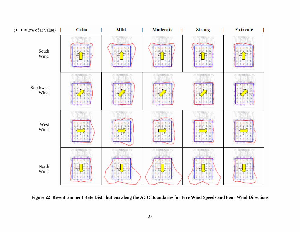
Figure 22 Re-entrainment Rate Distributions along the ACC Boundaries for Five Wind Speeds and Four Wind Directions

37

( = 2% of R value) South Wind Southwest Wind West Wind North Wind

However, increasing wind speed significantly changes this trend. As wind speed

increases, the wake size increases. When the wind is strong enough to pull the exhausted hot air

from ACC, the re-entrainment accordingly decreases. Accordingly, highest recirculation is

occurred at mid-level of upstream wind speed. This dependency of re-entrainment on wind

speed also was reported by experimental study of Gu et al. (2007), Slawson & Sullivan (1981),

and Hitchman & Slawson (1987) as well as Duvenhage and Kroger’s computational study (1996).

However, Kennedy and Fordyce (1974) have reported that strong wind speed stretches exhausted

plume long enough to reach air-inlet of the fan cells and accordingly increases recirculation.

Kennedy and Fordyce(1974) also showed the effect of wind speed on recirculation varies to the

densimetric Froude number. Because of the differences in modeling conditions for experimental

and numerical simulation of flow and heat transfer, the present and previous results show

somewhat different value of peak recirculation level and corresponding wind speed. However, it

is clearly agreed through all the research studies that wind speed strongly affects on the

recirculation process.

The size of the wake and according recirculation also are significantly affected by

geometric condition such as cooling tower configuration against wind and the space between

adjacent buildings and cooling tower. The dependency of re-entrainment on wind direction was

reported by Kennedy and Fordyce (1974) and Gu et al. (2007). They stated that the wind

blowing in the direction of the major axis of a heat exchanger results in a high recirculation of

hot plume. The north wind case in the present study showed the highest re-entrainment

distribution while the west and south-west directions resulted in much lower re-entrainment rates.

Figure 23 was presented in order to evaluate how the total re-entrainments rate depends

on the wind speed and direction. The wind speed in Figure 23 was converted from the category

values in Table 3 to meteorological tower height speeds. North wind has a significantly higher

re-entrainment rate than the rest of the wind directions. This is probably due to the power plant

buildings and facilities being located directly upwind of the ACC in the North wind direction

case. The peak values of total re-entrainment for the north wind direction were found in the mild

38

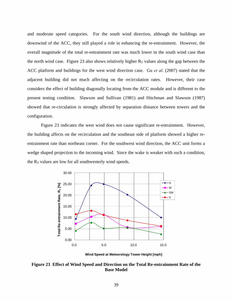
and moderate speed categories. For the south wind direction, although the buildings are

downwind of the ACC, they still played a role in enhancing the re-entrainment. However, the

overall magnitude of the total re-entrainment rate was much lower in the south wind case than

the north wind case. Figure 23 also shows relatively higher RT values along the gap between the

ACC platform and buildings for the west wind direction case. Gu et al. (2007) stated that the

adjacent building did not much affecting on the recirculation rates. However, their case

considers the effect of building diagonally locating from the ACC module and is different to the

present testing condition. Slawson and Sullivan (1981) and Hitchman and Slawson (1987)

showed that re-circulation is strongly affected by separation distance between towers and the

configuration.

Figure 23 indicates the west wind does not cause significant re-entrainment. However,

the building affects on the recirculation and the southeast side of platform showed a higher re-

entrainment rate than northeast corner. For the southwest wind direction, the ACC unit forms a

wedge shaped projection to the incoming wind. Since the wake is weaker with such a condition,

the RT values are low for all southwesterly wind speeds.

0.00

5.00

10.00

15.00

20.00

25.00

30.00

0.0 5.0 10.0 15.0

Tota

l Re-

entr

ainm

ent R

ate,

RT

[%]

Wind Speed at Meteorology Tower Height [mph]

N

W

SW

S

Figure 23 Effect of Wind Speed and Direction on the Total Re-entrainment Rate of the Base Model

39

Application of Meteorological Data

Although the testing results shown in Figures 21, 22, and 23 are useful to understand the

recirculation phenomenon around the ACC platform, they however are not what is actually

observed at the El Dorado site. This is because each of the result points was determined under

ideal conditions of a single wind direction and single wind speed, yet the real atmosphere

generally is much more complex than the ideally uniform wind-tunnel wind condition. Natural

wind at a particular location, such as El Dorado in this study, usually has a pattern that can be

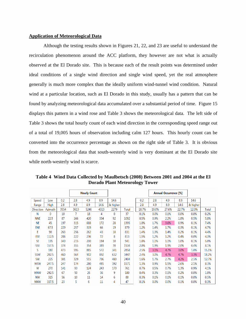
found by analyzing meteorological data accumulated over a substantial period of time. Figure 15

displays this pattern in a wind rose and Table 3 shows the meteorological data. The left side of

Table 3 shows the total hourly count of each wind direction in the corresponding speed range out

of a total of 19,005 hours of observation including calm 127 hours. This hourly count can be

converted into the occurrence percentage as shown on the right side of Table 3. It is obvious

from the meteorological data that south-westerly wind is very dominant at the El Dorado site

while north-westerly wind is scarce.

Table 4 Wind Data Collected by Maulbetsch (2008) Between 2001 and 2004 at the El Dorado Plant Meteorology Tower

40

In order to evaluate the actual re-entrainment level of the ACC, the wind occurrence

percentage data should be applied to the wind results of the wind-tunnel modeling. The

application of meteorological data is especially important in order to integrate the actual non-

ideal winds on site with the results of the tunnel modeling.

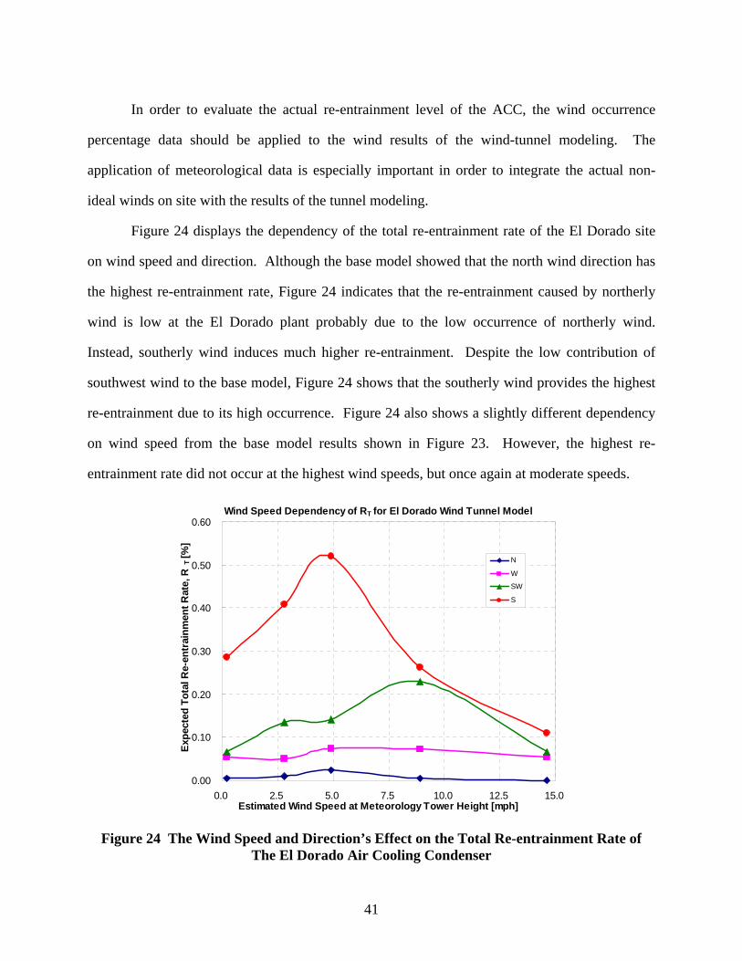
Figure 24 displays the dependency of the total re-entrainment rate of the El Dorado site

on wind speed and direction. Although the base model showed that the north wind direction has

the highest re-entrainment rate, Figure 24 indicates that the re-entrainment caused by northerly

wind is low at the El Dorado plant probably due to the low occurrence of northerly wind.

Instead, southerly wind induces much higher re-entrainment. Despite the low contribution of

southwest wind to the base model, Figure 24 shows that the southerly wind provides the highest

re-entrainment due to its high occurrence. Figure 24 also shows a slightly different dependency

on wind speed from the base model results shown in Figure 23. However, the highest re-

entrainment rate did not occur at the highest wind speeds, but once again at moderate speeds.

Wind Speed Dependency of RT for El Dorado Wind Tunnel Model

0.00

0.10

0.20

0.30

0.40

0.50

0.60

0.0 2.5 5.0 7.5 10.0 12.5 15.0Estimated Wind Speed at Meteorology Tower Height [mph]

Expe

cted

Tot

al R

e-en

trai

nmen

t Rat

e, R

T [%

]

N

W

SW

S

Figure 24 The Wind Speed and Direction’s Effect on the Total Re-entrainment Rate of The El Dorado Air Cooling Condenser

41

N

W RT=9.05% E

S

Scale : 0.2% Re-entrainment

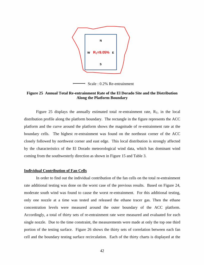
Figure 25 Annual Total Re-entrainment Rate of the El Dorado Site and the Distribution Along the Platform Boundary

Figure 25 displays the annually estimated total re-entrainment rate, RT, in the local

distribution profile along the platform boundary. The rectangle in the figure represents the ACC

platform and the curve around the platform shows the magnitude of re-entrainment rate at the

boundary cells. The highest re-entrainment was found on the northeast corner of the ACC

closely followed by northwest corner and east edge. This local distribution is strongly affected

by the characteristics of the El Dorado meteorological wind data, which has dominant wind

coming from the southwesterly direction as shown in Figure 15 and Table 3.

Individual Contribution of Fan Cells

In order to find out the individual contribution of the fan cells on the total re-entrainment

rate additional testing was done on the worst case of the previous results. Based on Figure 24,

moderate south wind was found to cause the worst re-entrainment. For this additional testing,

only one nozzle at a time was tested and released the ethane tracer gas. Then the ethane

concentration levels were measured around the outer boundary of the ACC platform.

Accordingly, a total of thirty sets of re-entrainment rate were measured and evaluated for each

single nozzle. Due to the time constraint, the measurements were made at only the top one third

portion of the testing surface. Figure 26 shows the thirty sets of correlation between each fan

cell and the boundary testing surface recirculation. Each of the thirty charts is displayed at the

42

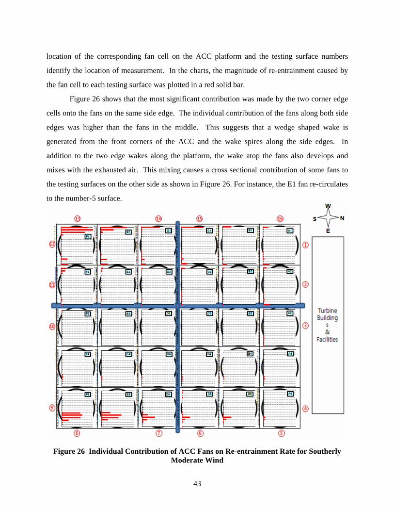
location of the corresponding fan cell on the ACC platform and the testing surface numbers

identify the location of measurement. In the charts, the magnitude of re-entrainment caused by

the fan cell to each testing surface was plotted in a red solid bar.

Figure 26 shows that the most significant contribution was made by the two corner edge

cells onto the fans on the same side edge. The individual contribution of the fans along both side

edges was higher than the fans in the middle. This suggests that a wedge shaped wake is

generated from the front corners of the ACC and the wake spires along the side edges. In

addition to the two edge wakes along the platform, the wake atop the fans also develops and

mixes with the exhausted air. This mixing causes a cross sectional contribution of some fans to

the testing surfaces on the other side as shown in Figure 26. For instance, the E1 fan re-circulates

to the number-5 surface.

Figure 26 Individual Contribution of ACC Fans on Re-entrainment Rate for Southerly Moderate Wind

43

44

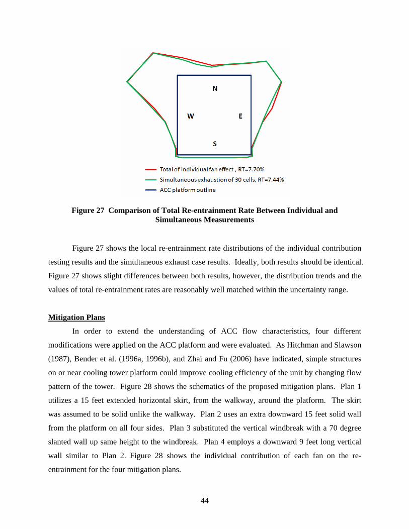
Figure 27 Comparison of Total Re-entrainment Rate Between Individual and Simultaneous Measurements

Figure 27 shows the local re-entrainment rate distributions of the individual contribution

testing results and the simultaneous exhaust case results. Ideally, both results should be identical.

Figure 27 shows slight differences between both results, however, the distribution trends and the

values of total re-entrainment rates are reasonably well matched within the uncertainty range.

Mitigation Plans

In order to extend the understanding of ACC flow characteristics, four different

modifications were applied on the ACC platform and were evaluated. As Hitchman and Slawson

(1987), Bender et al. (1996a, 1996b), and Zhai and Fu (2006) have indicated, simple structures

on or near cooling tower platform could improve cooling efficiency of the unit by changing flow

pattern of the tower. Figure 28 shows the schematics of the proposed mitigation plans. Plan 1

utilizes a 15 feet extended horizontal skirt, from the walkway, around the platform. The skirt

was assumed to be solid unlike the walkway. Plan 2 uses an extra downward 15 feet solid wall

from the platform on all four sides. Plan 3 substituted the vertical windbreak with a 70 degree

slanted wall up same height to the windbreak. Plan 4 employs a downward 9 feet long vertical

wall similar to Plan 2. Figure 28 shows the individual contribution of each fan on the re-

entrainment for the four mitigation plans.

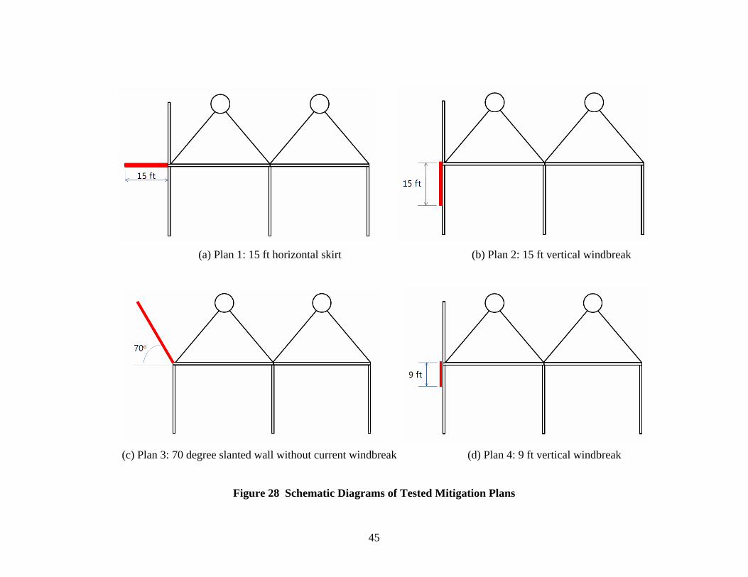
(a) Plan 1: 15 ft horizontal skirt (b) Plan 2: 15 ft vertical windbreak

(c) Plan 3: 70 degree slanted wall without current windbreak (d) Plan 4: 9 ft vertical windbreak

Figure 28 Schematic Diagrams of Tested Mitigation Plans

45

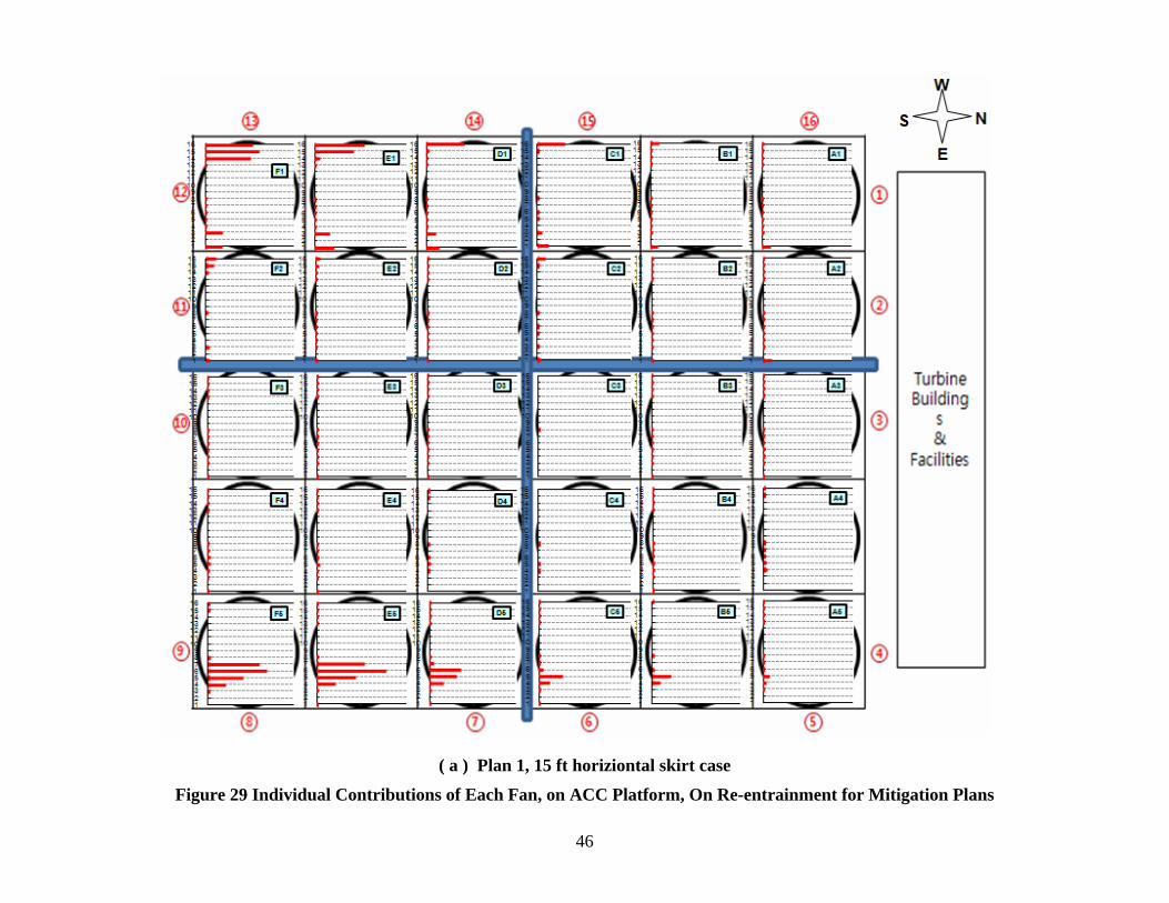
( a ) Plan 1, 15 ft horiziontal skirt case

Figure 29 Individual Contributions of Each Fan, on ACC Platform, On Re-entrainment for Mitigation Plans

46

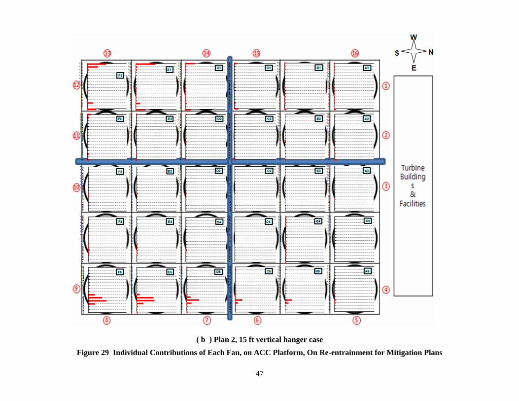
( b ) Plan 2, 15 ft vertical hanger case

Figure 29 Individual Contributions of Each Fan, on ACC Platform, On Re-entrainment for Mitigation Plans

47

( c ) Plan 3, 70 degree slanted wall atop the platform case

Figure 29 Individual Contributions of Each Fan, on ACC Platform, On Re-entrainment for Mitigation Plans

48

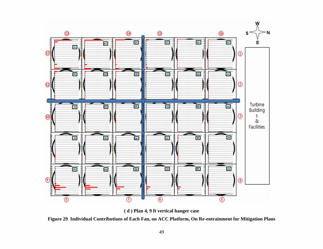
Figure 29 Individual Contributions of Each Fan, on ACC Platform, On Re-entrainment for Mitigation Plans

( d ) Plan 4, 9 ft vertical hanger case

49

The characteristics of all four mitigation plans were similar to the existing case, which was

shown in Figure 26 and explained previously. Among the four plans, the two vertical hanger

cases showed the largest decrease in overall re-entrainment. It was found that regardless of the

case, the largest re-entrainment came into the two outside back fans from the two front edge fans.

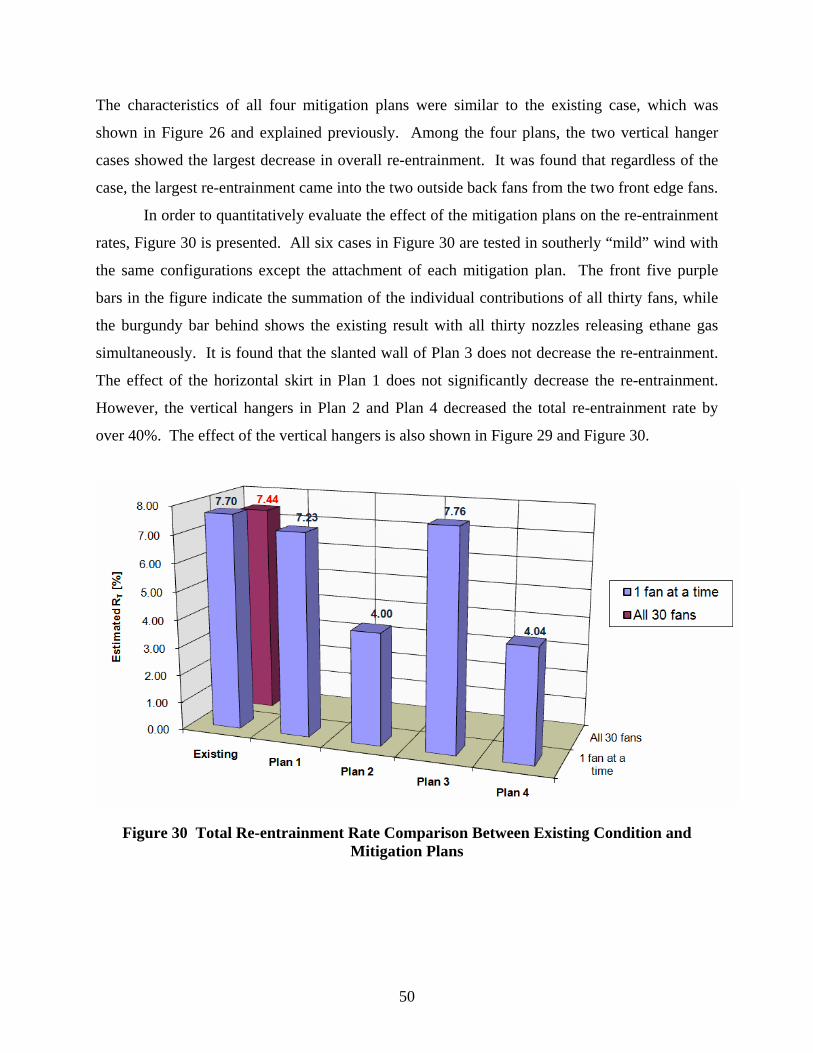
In order to quantitatively evaluate the effect of the mitigation plans on the re-entrainment

rates, Figure 30 is presented. All six cases in Figure 30 are tested in southerly “mild” wind with

the same configurations except the attachment of each mitigation plan. The front five purple

bars in the figure indicate the summation of the individual contributions of all thirty fans, while

the burgundy bar behind shows the existing result with all thirty nozzles releasing ethane gas

simultaneously. It is found that the slanted wall of Plan 3 does not decrease the re-entrainment.

The effect of the horizontal skirt in Plan 1 does not significantly decrease the re-entrainment.

However, the vertical hangers in Plan 2 and Plan 4 decreased the total re-entrainment rate by

over 40%. The effect of the vertical hangers is also shown in Figure 29 and Figure 30.

Figure 30 Total Re-entrainment Rate Comparison Between Existing Condition and Mitigation Plans

50

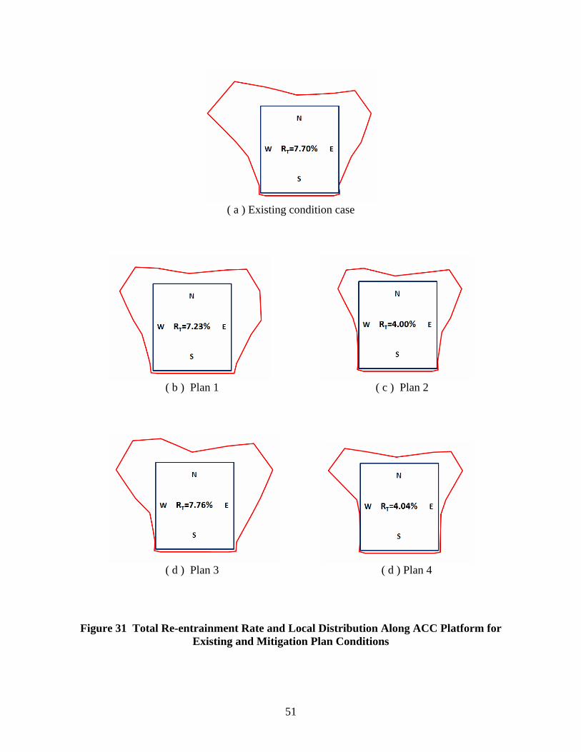
( a ) Existing condition case

( b ) Plan 1 ( c ) Plan 2

( d ) Plan 3 ( d ) Plan 4

Figure 31 Total Re-entrainment Rate and Local Distribution Along ACC Platform for Existing and Mitigation Plan Conditions

51

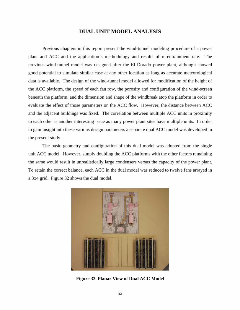
DUAL UNIT MODEL ANALYSIS

Previous chapters in this report present the wind-tunnel modeling procedure of a power

plant and ACC and the application’s methodology and results of re-entrainment rate. The

previous wind-tunnel model was designed after the El Dorado power plant, although showed

good potential to simulate similar case at any other location as long as accurate meteorological

data is available. The design of the wind-tunnel model allowed for modification of the height of

the ACC platform, the speed of each fan row, the porosity and configuration of the wind-screen

beneath the platform, and the dimension and shape of the windbreak atop the platform in order to

evaluate the effect of those parameters on the ACC flow. However, the distance between ACC

and the adjacent buildings was fixed. The correlation between multiple ACC units in proximity

to each other is another interesting issue as many power plant sites have multiple units. In order

to gain insight into these various design parameters a separate dual ACC model was developed in

the present study.

The basic geometry and configuration of this dual model was adopted from the single

unit ACC model. However, simply doubling the ACC platforms with the other factors remaining

the same would result in unrealistically large condensers versus the capacity of the power plant.

To retain the correct balance, each ACC in the dual model was reduced to twelve fans arrayed in

a 3x4 grid. Figure 32 shows the dual model.

Figure 32 Planar View of Dual ACC Model

52

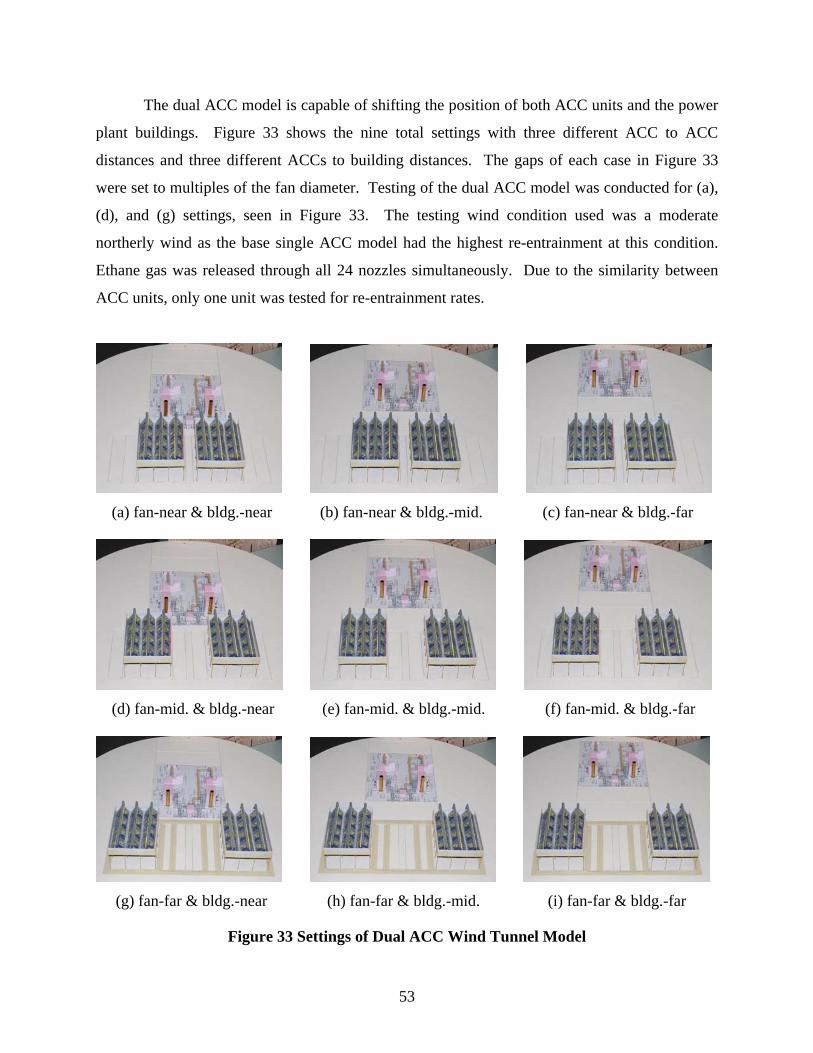
The dual ACC model is capable of shifting the position of both ACC units and the power

plant buildings. Figure 33 shows the nine total settings with three different ACC to ACC

distances and three different ACCs to building distances. The gaps of each case in Figure 33

were set to multiples of the fan diameter. Testing of the dual ACC model was conducted for (a),

(d), and (g) settings, seen in Figure 33. The testing wind condition used was a moderate

northerly wind as the base single ACC model had the highest re-entrainment at this condition.

Ethane gas was released through all 24 nozzles simultaneously. Due to the similarity between

ACC units, only one unit was tested for re-entrainment rates.

(a) fan-near & bldg.-near (b) fan-near & bldg.-mid. (c) fan-near & bldg.-far

(d) fan-mid. & bldg.-near (e) fan-mid. & bldg.-mid. (f) fan-mid. & bldg.-far

(g) fan-far & bldg.-near (h) fan-far & bldg.-mid. (i) fan-far & bldg.-far

Figure 33 Settings of Dual ACC Wind Tunnel Model

53

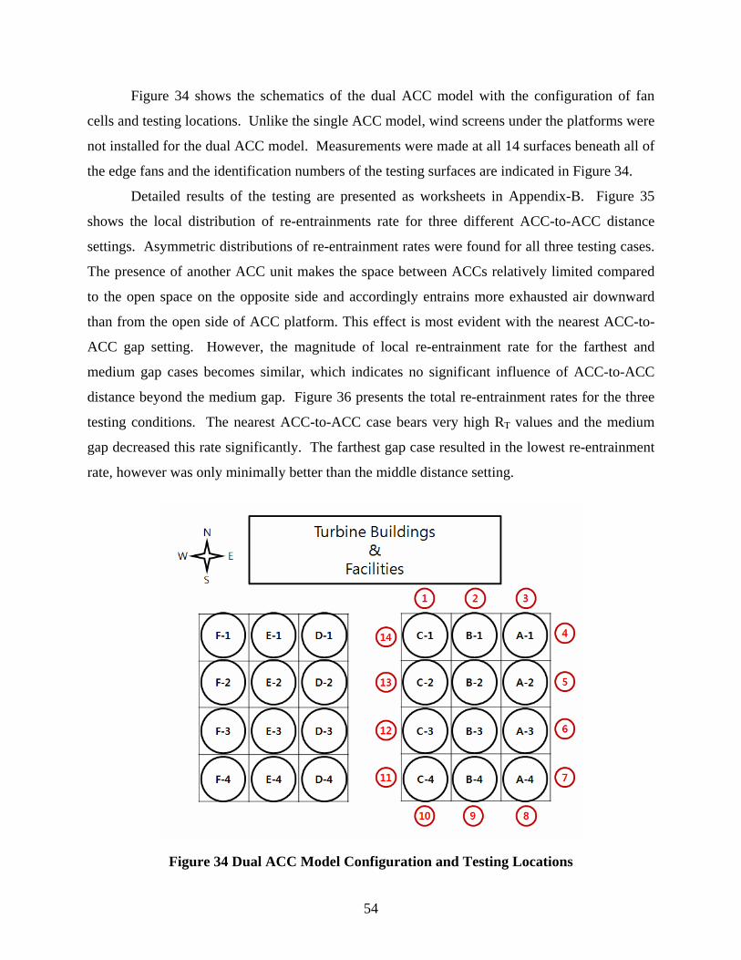
Figure 34 shows the schematics of the dual ACC model with the configuration of fan

cells and testing locations. Unlike the single ACC model, wind screens under the platforms were

not installed for the dual ACC model. Measurements were made at all 14 surfaces beneath all of

the edge fans and the identification numbers of the testing surfaces are indicated in Figure 34.

Detailed results of the testing are presented as worksheets in Appendix-B. Figure 35

shows the local distribution of re-entrainments rate for three different ACC-to-ACC distance

settings. Asymmetric distributions of re-entrainment rates were found for all three testing cases.

The presence of another ACC unit makes the space between ACCs relatively limited compared

to the open space on the opposite side and accordingly entrains more exhausted air downward

than from the open side of ACC platform. This effect is most evident with the nearest ACC-to-

ACC gap setting. However, the magnitude of local re-entrainment rate for the farthest and

medium gap cases becomes similar, which indicates no significant influence of ACC-to-ACC

distance beyond the medium gap. Figure 36 presents the total re-entrainment rates for the three

testing conditions. The nearest ACC-to-ACC case bears very high RT values and the medium

gap decreased this rate significantly. The farthest gap case resulted in the lowest re-entrainment

rate, however was only minimally better than the middle distance setting.

Figure 34 Dual ACC Model Configuration and Testing Locations

54

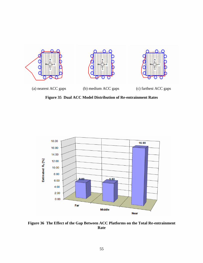
(a) nearest ACC gaps (b) medium ACC gaps (c) farthest ACC gaps

Figure 35 Dual ACC Model Distribution of Re-entrainment Rates

Figure 36 The Effect of the Gap Between ACC Platforms on the Total Re-entrainment Rate

55

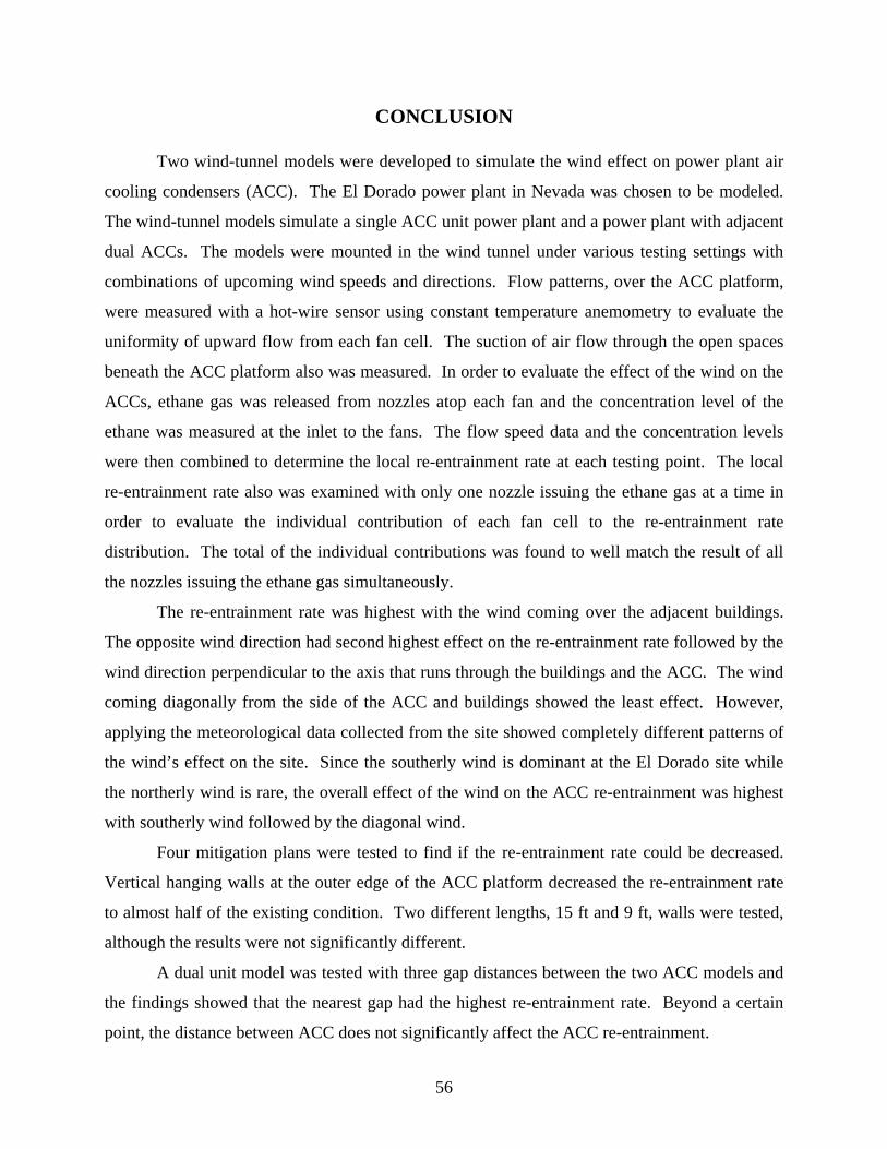
CONCLUSION

Two wind-tunnel models were developed to simulate the wind effect on power plant air

cooling condensers (ACC). The El Dorado power plant in Nevada was chosen to be modeled.

The wind-tunnel models simulate a single ACC unit power plant and a power plant with adjacent

dual ACCs. The models were mounted in the wind tunnel under various testing settings with

combinations of upcoming wind speeds and directions. Flow patterns, over the ACC platform,

were measured with a hot-wire sensor using constant temperature anemometry to evaluate the

uniformity of upward flow from each fan cell. The suction of air flow through the open spaces

beneath the ACC platform also was measured. In order to evaluate the effect of the wind on the

ACCs, ethane gas was released from nozzles atop each fan and the concentration level of the

ethane was measured at the inlet to the fans. The flow speed data and the concentration levels

were then combined to determine the local re-entrainment rate at each testing point. The local

re-entrainment rate also was examined with only one nozzle issuing the ethane gas at a time in

order to evaluate the individual contribution of each fan cell to the re-entrainment rate

distribution. The total of the individual contributions was found to well match the result of all

the nozzles issuing the ethane gas simultaneously.

The re-entrainment rate was highest with the wind coming over the adjacent buildings.

The opposite wind direction had second highest effect on the re-entrainment rate followed by the

wind direction perpendicular to the axis that runs through the buildings and the ACC. The wind

coming diagonally from the side of the ACC and buildings showed the least effect. However,

applying the meteorological data collected from the site showed completely different patterns of

the wind’s effect on the site. Since the southerly wind is dominant at the El Dorado site while

the northerly wind is rare, the overall effect of the wind on the ACC re-entrainment was highest

with southerly wind followed by the diagonal wind.

Four mitigation plans were tested to find if the re-entrainment rate could be decreased.

Vertical hanging walls at the outer edge of the ACC platform decreased the re-entrainment rate

to almost half of the existing condition. Two different lengths, 15 ft and 9 ft, walls were tested,

although the results were not significantly different.

A dual unit model was tested with three gap distances between the two ACC models and

the findings showed that the nearest gap had the highest re-entrainment rate. Beyond a certain

point, the distance between ACC does not significantly affect the ACC re-entrainment.

56

ACKNOWLEDGEMENTS

The authors are deeply grateful to Dr. Charles McGowin of EPRI for his generous

support and patience for last two years of project. We wish to acknowledge that Dr. John

Maulbetsch of Maulbetsch Consulting has been providing very helpful discussion and his field

measurement experience. The meteorology data and plant conditions of El Dorado site were

provided by Dr. Maulbetsch and Mr. Michael Spaulding, a former Plant Engineer of El Dorado

Energy LLC. Mr. Franck David of EdF (Électricité de France) has shared his computational

simulation results of single and dual air cooling condenser units with us. Dr. Robert Goldstein

and other great researchers of EPRI have given us valuable comments so we could analyze the

results more appropriately. Miss Bethany Kuspa, a former manager of U.C. Davis ABLWT

laboratory, deserves special appreciation for her effort at the beginning stage of this project.

U.C. Davis students Mr. Ashishkumar Patel and Mr. Justin Tucker have been great helpers to

conduct huge hours of modeling and testing. Mrs. Yoke Dellenback, Mrs. Sharon Holgerson,

and Mrs. Denyse Miller in Department of Mechanical and Aerospace Engineering of U.C. Davis

have handled various administrative affairs smoothly and allowed us to concentrate on the

engineering work of this project. The authors sincerely thank to each of these colleagues and

friends.

57

REFERENCES

Rafat Al-Waked and Masud Behnia, “The performance of natural draft dry cooling towers under crosswind: CFD study,” Int. J. Energy Research, Vol. 28, pp. 147-161, 2004

T.J. Bender, D.J. Bergstrom, and K.S. Rezhallah, “A study on the effects of wind on the air intake flow rate of a cooling tower: Part 2. Wind wall study,” J. Wind Engineering and Industrial Aerodynamics, Vol. 64, pp.61-72, 1996a

T.J. Bender, D.J. Bergstrom, and K.S. Rezhallah, “A study on the effects of wind on the air intake flow rate of a cooling tower: Part 3. Numerical study,” J. Wind Engineering and Industrial Aerodynamics, Vol. 64, pp.73-88, 1996b

R.B. Bornoff and M.R. Mokhtarzadeh-Dehghan, “A numerical study of interacting buoyant cooling-tower plumes,” Atmospheric Environment, Vol.35, pp.589-598, 2001

D. Derksen, K.S. Rezhallah, and D.J. Bergstron, “A wind tunnel study of the effect of wind on the air intake of a cooling tower,” ASME Measurement and Modeling of Environmental Flows, FED-Vol.143/HTD-Vol.232, pp. 171-176, 1992

D.D. Derksen, T.J. Bender, D.J. Bergstrom, and K.S. Rezhallah, “A study on the effects of wind on the air intake flow rate of a cooling tower: Part 1. Wind tunnel study,” J. Wind Engineering and Industrial Aerodynamics, Vol. 64, pp.47-59, 1996

A.F. du Preez and D.G. Kröger, “Effect of wind on performance of a dry-cooling tower,” Heat Recovery systems & CHP, Vol. 13, No.2, pp.139-146, 1993

A.F. du Preez and D.G. Kröger, “Effect of the shape of the tower supports and walls on the performance of a dry -cooling tower subjected to cross winds,” Heat Transfer Engineering, Vol. 16, No.2, pp.42-49, 1995

A.F. du Preez and D.G. Kröger, “The effect of the heat exchanger arrangement and wind-break walls on the performance of natural draft dry-cooling towers subjected to cross-winds,” J. Wind Engineering and Industrial Aerodynamics, Vol. 58, pp.293-303, 1995

K. Duvenhage and D.G. Kröger, “The influence of wind on the performance of forced draught air-cooled heat exchangers,” J. Wind Engineering and Industrial Aerodynamics, Vol. 62, pp.259-277, 1996

Zhifu Gu, Hui Li, Wenhong Zhang, Yan Li, and Jiye Peng, “Wind tunnel simulation on re-circulation of air-cooled condensers of a power plant,” J. Wind Engineering and Industrial Aerodynamics, Vol.93, pp.509-520, 2005

Zhifu Gu, Xuerei Chen, William Lubitz, Yan Li, and Wenlin Luo, “Wind tunnel simulation of exhaust recirculation in an air-cooling system at a large power plant,” Int. J. Thermal Sciences, V.46, No.3, pp.308-317, 2007

58

G.J. Hitchman and P.R. Slawson, “An experimental investigation of recirculation and interference on modeled forced-draft round cooling towers,” J. Engineering for Gas Turbines and Power, Vol.109, pp.124-125, 1987

N. Isymov and H. Tanaka, “Wind tunnel modeling of stack gas dispersion – Difficulties and approximations,” Proceedings of Fifth Int. Conf. on Wind Engineering July 8-14 1979, Colorado State University, Vol. II, pp.VIII-3-1 to 15.

M. Jensen, “The model-law for phenomena in natural wind,” Ingeniøren (International Edition) , Vol. 2, No. 4, 1958

C.G. Justus and Amir Mikhail, “Height variation of wind speed and wind distributions statistics,” Geophysical Research Letters, Vol. 3, No. 5, pp.261-264, 1976

John F. Kennedy and Homer Fordyce, “Plume recirculation and interference in mechanical-draft cooling towers,” Proceedings of Cooling Tower Environment-1974 Symposium March 4-6, pp.58-87, 1974

Detlev G. Kröger, “Air-cooled heat exchangers and cooling towers; Thermal-flow performance evaluation and design,” Volume II, 2004

John S. Maulbetsch, personal communication and field measurement data, 2008

P. R. Slawson and H. F. Sullivan, “Model studies on the design and arrangement of forced draft cooling towers to minimize recirculation and interference,” Waste heat, utilization and management, Proceeding of Miami Beach Conference May 11-13, 1981, pp. 235- proceeding, 1981

William H. Snyder, “Guideline for fluid modeling of atmospheric diffusion,” US EPA Report No.EPA-600/8-81-009, 1981

M.D. Su, G.F. Tang, and S. Fu, “Numerical simulation of fluid flow and thermal performance of a dry-cooling tower under cross wind condition,” J. Wind Engineering and Industrial Aerodynamics, Vol. 79, pp. 289-306, 1999

O.G. Sutton, “Atmospheric Turbulence,” 1949

Q. Wei, B. Zhang, K.Liu, X. Du, and X. Meng, “A study of the unfavorable effects of wind on the cooling efficiency of dry cooling towers,” J. Wind Engineering and Industrial Aerodynamics, Vol. 54/55, pp. 633-643, 1995

Z. Zhai and S. Fu, “Improving cooling efficiency of dry-cooling towers under cross-wind conditions by using wind-break methods,” Applied Thermal Engineering, Vol. 26, pp. 1008-1017, 2006

59

60

APPENDIX

Appendix –A Testing Results of the Single Unit Base Model

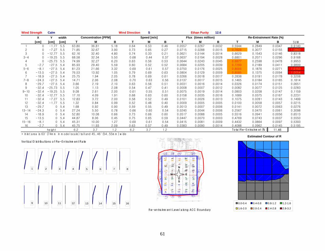
Wind Strength Wind Direction Ethan Purity

0.7628

0.6877

0.7299

0.8006

0.8585

Calm S 12.6X Y width

[cm] [cm] [cm] T M B T M B T M B T M B SU M

1 0 -1.77 5.5 63.80 36.81 5.18 0.64 0.53 0.46 0.0557 0.0267 0.0032 0.5944 0.2849 0.0347 0.91402 0 -7.27 5.5 71.85 32.67 3.90 0.73 0.65 0.27 0.0715 0.0288 0.0015 0.3077 0.0155 1.0860

3 0 -12.77 5.5 62.16 32.40 4.80 0.74 0.33 0.21 0.0621 0.0144 0.0014 0.6629 0.1543 0.0146 0.8318

3-4 0 -19.25 5.5 68.58 32.34 5.50 0.68 0.44 0.37 0.0637 0.0194 0.0028 0.6801 0.2071 0.0296 0.9168

4 0 -25.73 5.5 74.99 32.27 6.20 0.63 0.56 0.53 0.0644 0.0243 0.0045 0.2598 0.0478 0.9953

5 -2.7 -27.5 5.4 85.93 29.40 5.59 0.60 0.52 0.52 0.0684 0.0205 0.0039 0.2189 0.0411 0.9899

5-6 -8.1 -27.5 5.4 81.23 21.66 3.32 0.69 0.61 0.57 0.0750 0.0176 0.0025 0.1876 0.0271 1.0153

6 -13.5 -27.5 5.4 76.53 13.92 1.05 0.79 0.69 0.63 0.0804 0.0129 0.0009 0.1375 0.0094 1.00547 -18.9 -27.5 5.4 25.75 1.94 2.05 0.78 0.69 0.61 0.0266 0.0018 0.0017 0.2838 0.0191 0.0178 0.3208

7-8 -24.3 -27.5 5.4 14.71 2.06 2.08 0.70 0.63 0.56 0.0137 0.0017 0.0015 0.1465 0.0184 0.0165 0.1814

8 -29.7 -27.5 5.4 3.66 2.19 2.10 0.63 0.56 0.51 0.0031 0.0016 0.0014 0.0326 0.0174 0.0151 0.0651

9 -32.4 -25.73 5.5 1.05 1.13 2.08 0.54 0.47 0.41 0.0008 0.0007 0.0012 0.0082 0.0077 0.0125 0.0283

9-10 -32.4 -19.25 5.5 9.08 2.61 2.00 0.61 0.55 0.51 0.0075 0.0019 0.0014 0.0803 0.0208 0.0147 0.1159

10 -32.4 -12.77 5.5 17.10 4.09 1.91 0.68 0.63 0.60 0.0158 0.0035 0.0016 0.1689 0.0375 0.0167 0.223111 -32.4 -7.27 5.5 12.83 3.72 2.00 0.58 0.52 0.49 0.0101 0.0026 0.0013 0.1075 0.0281 0.0143 0.1499

12 -32.4 -1.77 5.5 1.32 0.84 0.99 0.52 0.48 0.40 0.0009 0.0005 0.0005 0.0100 0.0058 0.0057 0.0215

13 -29.7 0 5.4 1.68 0.92 0.90 0.59 0.55 0.49 0.0013 0.0007 0.0006 0.0141 0.0072 0.0063 0.0276

13-14 -24.3 0 5.4 27.24 5.50 0.78 0.66 0.60 0.54 0.0240 0.0044 0.0006 0.2567 0.0470 0.0061 0.3098

14 -18.9 0 5.4 52.80 10.08 0.66 0.73 0.66 0.60 0.0517 0.0088 0.0005 0.5516 0.0941 0.0056 0.6513

15 -13.5 0 5.4 44.87 8.06 0.45 0.75 0.65 0.59 0.0447 0.0070 0.0003 0.4769 0.0743 0.0037 0.5550

15-16 -8.1 0 5.4 45.31 10.00 1.27 0.69 0.61 0.54 0.0415 0.0081 0.0009 0.4432 0.0864 0.0097 0.539316 -2.7 0 5.4 45.75 11.93 2.09 0.63 0.57 0.49 0.0383 0.0090 0.0014 0.4088 0.0962 0.0145 0.5195

height 6.2 3.7 1.2 6.2 3.7 1.2 11.46

* Inlet area is 63' (74m m in m odel scale) tall and 45, 46' (54, 55m m ) w ide

Vertical D istributions of R e-Entrainm ent R ate

R e-entrainm ent Level along A C C B oundary

Total R e-Entrainm et (% )

Re-Entrainment Rate (%)Concentration [PPM] Speed [m/s] Flux (times million)

1 2 3 4 5 6 7 8

9 10 11 12 13 14 15 16

N

E

S

W

Estimated Contour of R

0.0-0.4 0.4-0.8 0.8-1.2 1.2-1.6

1.6-2.0 2.0-2.4 2.4-2.8 2.8-3.2

61

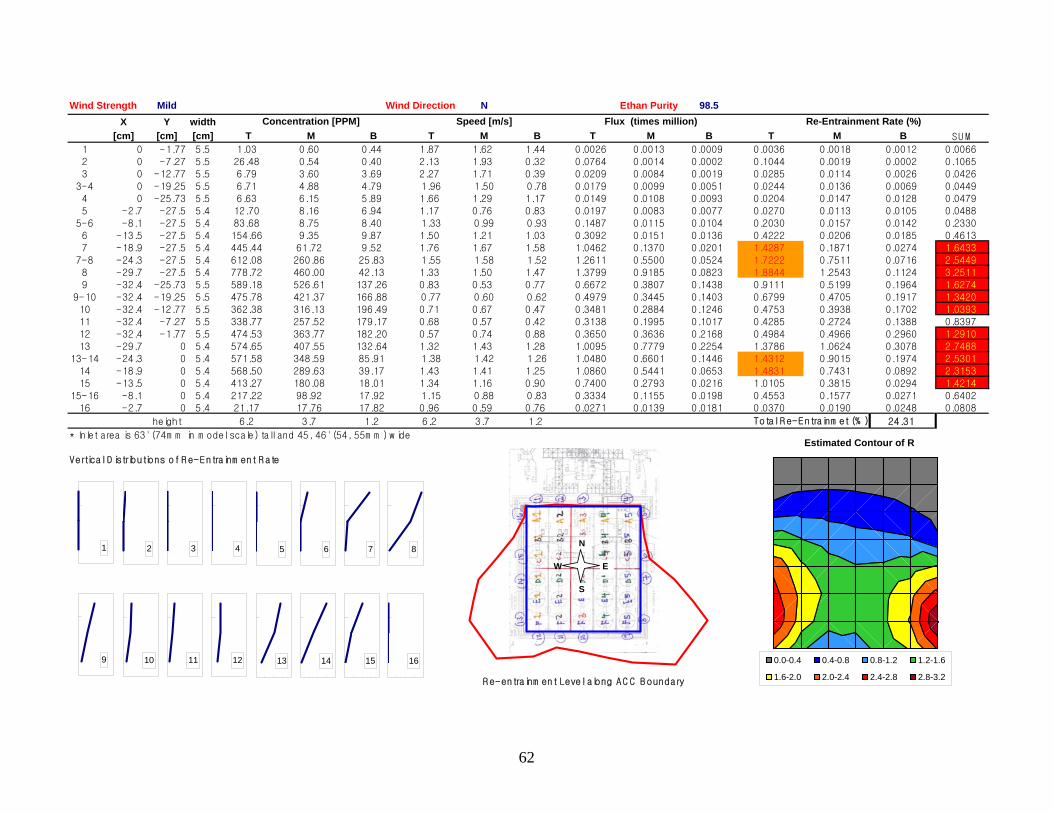
Wind Strength Wind Direction Ethan Purity

1.4287

1.72221.8844

1.4312

1.4831

Mild N 98.5X Y width

[cm] [cm] [cm] T M B T M B T M B T M B SU M

1 0 -1.77 5.5 1.03 0.60 0.44 1.87 1.62 1.44 0.0026 0.0013 0.0009 0.0036 0.0018 0.0012 0.00662 0 -7.27 5.5 26.48 0.54 0.40 2.13 1.93 0.32 0.0764 0.0014 0.0002 0.1044 0.0019 0.0002 0.10653 0 -12.77 5.5 6.79 3.60 3.69 2.27 1.71 0.39 0.0209 0.0084 0.0019 0.0285 0.0114 0.0026 0.0426

3-4 0 -19.25 5.5 6.71 4.88 4.79 1.96 1.50 0.78 0.0179 0.0099 0.0051 0.0244 0.0136 0.0069 0.04494 0 -25.73 5.5 6.63 6.15 5.89 1.66 1.29 1.17 0.0149 0.0108 0.0093 0.0204 0.0147 0.0128 0.04795 -2.7 -27.5 5.4 12.70 8.16 6.94 1.17 0.76 0.83 0.0197 0.0083 0.0077 0.0270 0.0113 0.0105 0.0488

5-6 -8.1 -27.5 5.4 83.68 8.75 8.40 1.33 0.99 0.93 0.1487 0.0115 0.0104 0.2030 0.0157 0.0142 0.23306 -13.5 -27.5 5.4 154.66 9.35 9.87 1.50 1.21 1.03 0.3092 0.0151 0.0136 0.4222 0.0206 0.0185 0.46137 -18.9 -27.5 5.4 445.44 61.72 9.52 1.76 1.67 1.58 1.0462 0.1370 0.0201 0.1871 0.0274 1.6433

7-8 -24.3 -27.5 5.4 612.08 260.86 25.83 1.55 1.58 1.52 1.2611 0.5500 0.0524 0.7511 0.0716 2.54498 -29.7 -27.5 5.4 778.72 460.00 42.13 1.33 1.50 1.47 1.3799 0.9185 0.0823 1.2543 0.1124 3.25119 -32.4 -25.73 5.5 589.18 526.61 137.26 0.83 0.53 0.77 0.6672 0.3807 0.1438 0.9111 0.5199 0.1964 1.6274

9-10 -32.4 -19.25 5.5 475.78 421.37 166.88 0.77 0.60 0.62 0.4979 0.3445 0.1403 0.6799 0.4705 0.1917 1.342010 -32.4 -12.77 5.5 362.38 316.13 196.49 0.71 0.67 0.47 0.3481 0.2884 0.1246 0.4753 0.3938 0.1702 1.039311 -32.4 -7.27 5.5 338.77 257.52 179.17 0.68 0.57 0.42 0.3138 0.1995 0.1017 0.4285 0.2724 0.1388 0.8397

12 -32.4 -1.77 5.5 474.53 363.77 182.20 0.57 0.74 0.88 0.3650 0.3636 0.2168 0.4984 0.4966 0.2960 1.291013 -29.7 0 5.4 574.65 407.55 132.64 1.32 1.43 1.28 1.0095 0.7779 0.2254 1.3786 1.0624 0.3078 2.7488

13-14 -24.3 0 5.4 571.58 348.59 85.91 1.38 1.42 1.26 1.0480 0.6601 0.1446 0.9015 0.1974 2.5301

14 -18.9 0 5.4 568.50 289.63 39.17 1.43 1.41 1.25 1.0860 0.5441 0.0653 0.7431 0.0892 2.315315 -13.5 0 5.4 413.27 180.08 18.01 1.34 1.16 0.90 0.7400 0.2793 0.0216 1.0105 0.3815 0.0294 1.4214

15-16 -8.1 0 5.4 217.22 98.92 17.92 1.15 0.88 0.83 0.3334 0.1155 0.0198 0.4553 0.1577 0.0271 0.640216 -2.7 0 5.4 21.17 17.76 17.82 0.96 0.59 0.76 0.0271 0.0139 0.0181 0.0370 0.0190 0.0248 0.0808

height 6.2 3.7 1.2 6.2 3.7 1.2 24.31

* Inlet area is 63' (74m m in m odel scale) tall and 45, 46' (54, 55m m ) w ide

Vertical D istributions of R e-Entrainm ent R ate

R e-entrainm ent Level along AC C B oundary

Total R e-Entrainm et (% )

Re-Entrainment Rate (%)Concentration [PPM] Speed [m/s] Flux (times million)

1 2 3 4 5 6 7 8

9 10 11 12 13 14 15 16

N

E

S

W

Estimated Contour of R

0.0-0.4 0.4-0.8 0.8-1.2 1.2-1.6

1.6-2.0 2.0-2.4 2.4-2.8 2.8-3.2

62

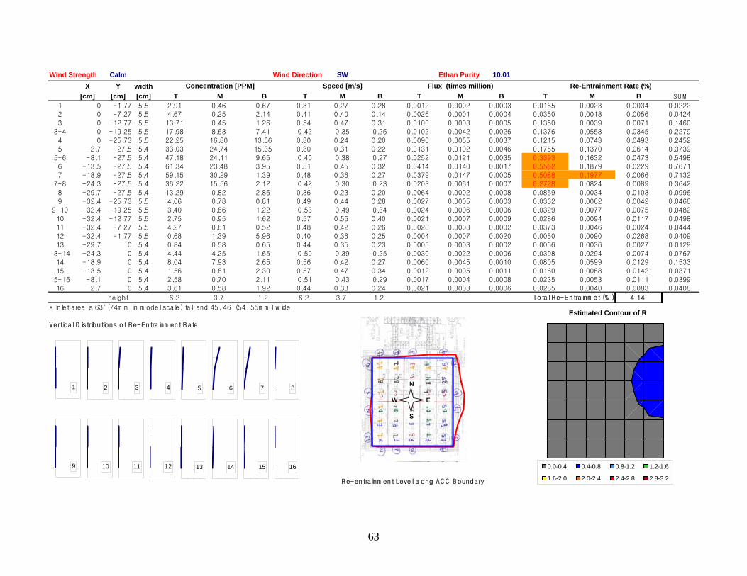
Wind Strength Wind Direction Ethan Purity

0.3393

0.55620.5088 0.1977

0.2728

Calm SW 10.01X Y width

[cm] [cm] [cm] T M B T M B T M B T M B SU M

1 0 -1.77 5.5 2.91 0.46 0.67 0.31 0.27 0.28 0.0012 0.0002 0.0003 0.0165 0.0023 0.0034 0.02222 0 -7.27 5.5 4.67 0.25 2.14 0.41 0.40 0.14 0.0026 0.0001 0.0004 0.0350 0.0018 0.0056 0.0424

3 0 -12.77 5.5 13.71 0.45 1.26 0.54 0.47 0.31 0.0100 0.0003 0.0005 0.1350 0.0039 0.0071 0.1460

3-4 0 -19.25 5.5 17.98 8.63 7.41 0.42 0.35 0.26 0.0102 0.0042 0.0026 0.1376 0.0558 0.0345 0.2279

4 0 -25.73 5.5 22.25 16.80 13.56 0.30 0.24 0.20 0.0090 0.0055 0.0037 0.1215 0.0743 0.0493 0.2452

5 -2.7 -27.5 5.4 33.03 24.74 15.35 0.30 0.31 0.22 0.0131 0.0102 0.0046 0.1755 0.1370 0.0614 0.3739

5-6 -8.1 -27.5 5.4 47.18 24.11 9.65 0.40 0.38 0.27 0.0252 0.0121 0.0035 0.1632 0.0473 0.5498

6 -13.5 -27.5 5.4 61.34 23.48 3.95 0.51 0.45 0.32 0.0414 0.0140 0.0017 0.1879 0.0229 0.76717 -18.9 -27.5 5.4 59.15 30.29 1.39 0.48 0.36 0.27 0.0379 0.0147 0.0005 0.0066 0.7132

7-8 -24.3 -27.5 5.4 36.22 15.56 2.12 0.42 0.30 0.23 0.0203 0.0061 0.0007 0.0824 0.0089 0.3642

8 -29.7 -27.5 5.4 13.29 0.82 2.86 0.36 0.23 0.20 0.0064 0.0002 0.0008 0.0859 0.0034 0.0103 0.0996

9 -32.4 -25.73 5.5 4.06 0.78 0.81 0.49 0.44 0.28 0.0027 0.0005 0.0003 0.0362 0.0062 0.0042 0.0466

9-10 -32.4 -19.25 5.5 3.40 0.86 1.22 0.53 0.49 0.34 0.0024 0.0006 0.0006 0.0329 0.0077 0.0075 0.0482

10 -32.4 -12.77 5.5 2.75 0.95 1.62 0.57 0.55 0.40 0.0021 0.0007 0.0009 0.0286 0.0094 0.0117 0.049811 -32.4 -7.27 5.5 4.27 0.61 0.52 0.48 0.42 0.26 0.0028 0.0003 0.0002 0.0373 0.0046 0.0024 0.0444

12 -32.4 -1.77 5.5 0.68 1.39 5.96 0.40 0.36 0.25 0.0004 0.0007 0.0020 0.0050 0.0090 0.0268 0.0409

13 -29.7 0 5.4 0.84 0.58 0.65 0.44 0.35 0.23 0.0005 0.0003 0.0002 0.0066 0.0036 0.0027 0.0129

13-14 -24.3 0 5.4 4.44 4.25 1.65 0.50 0.39 0.25 0.0030 0.0022 0.0006 0.0398 0.0294 0.0074 0.0767

14 -18.9 0 5.4 8.04 7.93 2.65 0.56 0.42 0.27 0.0060 0.0045 0.0010 0.0805 0.0599 0.0129 0.1533

15 -13.5 0 5.4 1.56 0.81 2.30 0.57 0.47 0.34 0.0012 0.0005 0.0011 0.0160 0.0068 0.0142 0.0371

15-16 -8.1 0 5.4 2.58 0.70 2.11 0.51 0.43 0.29 0.0017 0.0004 0.0008 0.0235 0.0053 0.0111 0.039916 -2.7 0 5.4 3.61 0.58 1.92 0.44 0.38 0.24 0.0021 0.0003 0.0006 0.0285 0.0040 0.0083 0.0408

height 6.2 3.7 1.2 6.2 3.7 1.2 4.14

* Inlet area is 63' (74m m in m odel scale) tall and 45, 46' (54, 55m m ) w ide

Vertical D istributions of R e-Entrainm ent R ate

R e-entrainm ent Level along A C C B oundary

Total R e-Entrainm et (% )

Re-Entrainment Rate (%)Concentration [PPM] Speed [m/s] Flux (times million)

1 2 3 4 5 6 7 8

9 10 11 12 13 14 15 16

N

E

S

W

Estimated Contour of R

0.0-0.4 0.4-0.8 0.8-1.2 1.2-1.6

1.6-2.0 2.0-2.4 2.4-2.8 2.8-3.2

63

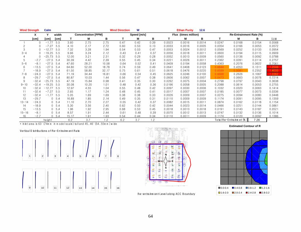
Wind Strength Wind Direction Ethan Purity

0.68440.6599 0.5081

0.6668

0.6473

0.2798

Calm W 12.6X Y width

[cm] [cm] [cm] T M B T M B T M B T M B SU M

1 0 -1.77 5.5 3.60 2.75 2.75 0.47 0.42 0.39 0.0023 0.0016 0.0014 0.0247 0.0168 0.0154 0.05682 0 -7.27 5.5 4.10 2.17 2.72 0.60 0.53 0.13 0.0033 0.0016 0.0005 0.0354 0.0166 0.0053 0.0572

3 0 -12.77 5.5 7.32 3.28 1.94 0.54 0.53 0.47 0.0053 0.0024 0.0012 0.0569 0.0252 0.0133 0.0954

3-4 0 -19.25 5.5 9.66 3.24 2.12 0.43 0.41 0.37 0.0056 0.0018 0.0011 0.0600 0.0194 0.0115 0.0909

4 0 -25.73 5.5 12.00 3.21 2.31 0.32 0.29 0.28 0.0052 0.0013 0.0009 0.0560 0.0136 0.0092 0.0788

5 -2.7 -27.5 5.4 30.39 4.42 2.39 0.55 0.45 0.34 0.0221 0.0026 0.0011 0.2362 0.0281 0.0114 0.2757

5-6 -8.1 -27.5 5.4 47.60 28.21 10.58 0.64 0.52 0.41 0.0409 0.0194 0.0058 0.4363 0.2076 0.0622 0.7061

6 -13.5 -27.5 5.4 64.80 52.00 18.78 0.74 0.59 0.49 0.0641 0.0408 0.0123 0.4350 0.1311 1.25067 -18.9 -27.5 5.4 61.50 58.85 32.17 0.75 0.61 0.51 0.0618 0.0476 0.0220 0.2352 1.4033

7-8 -24.3 -27.5 5.4 71.19 34.44 16.81 0.66 0.54 0.45 0.0625 0.0246 0.0100 0.2626 0.1067 1.0362

8 -29.7 -27.5 5.4 80.87 10.03 1.44 0.56 0.47 0.38 0.0606 0.0062 0.0007 0.0663 0.0078 0.7214

9 -32.4 -25.73 5.5 47.19 15.84 0.98 0.41 0.35 0.30 0.0262 0.0075 0.0004 0.0797 0.0043 0.3638

9-10 -32.4 -19.25 5.5 30.08 10.20 1.01 0.48 0.42 0.36 0.0196 0.0058 0.0005 0.2088 0.0614 0.0053 0.2755

10 -32.4 -12.77 5.5 12.97 4.55 1.04 0.55 0.48 0.42 0.0097 0.0030 0.0006 0.1032 0.0320 0.0063 0.141411 -32.4 -7.27 5.5 2.65 1.17 1.24 0.48 0.45 0.41 0.0017 0.0007 0.0007 0.0185 0.0077 0.0073 0.0336

12 -32.4 -1.77 5.5 5.05 1.69 1.69 0.38 0.38 0.33 0.0026 0.0009 0.0007 0.0275 0.0094 0.0080 0.0448

13 -29.7 0 5.4 16.89 1.85 2.14 0.49 0.35 0.31 0.0110 0.0009 0.0009 0.1174 0.0091 0.0095 0.1359

13-14 -24.3 0 5.4 11.10 2.70 2.27 0.55 0.42 0.37 0.0082 0.0015 0.0011 0.0874 0.0162 0.0118 0.1154

14 -18.9 0 5.4 5.30 3.56 2.40 0.62 0.50 0.42 0.0044 0.0023 0.0014 0.0466 0.0251 0.0144 0.0861

15 -13.5 0 5.4 1.96 1.92 2.95 0.68 0.53 0.45 0.0018 0.0013 0.0018 0.0191 0.0143 0.0187 0.0521

15-16 -8.1 0 5.4 8.57 1.91 2.44 0.61 0.48 0.39 0.0070 0.0012 0.0013 0.0747 0.0132 0.0136 0.101416 -2.7 0 5.4 15.17 1.91 1.93 0.54 0.44 0.34 0.0110 0.0011 0.0009 0.1174 0.0120 0.0092 0.1386

height 6.2 3.7 1.2 6.2 3.7 1.2 7.26

* Inlet area is 63' (74m m in m odel scale) tall and 45, 46' (54, 55m m ) w ide

Vertical D istributions of R e-Entrainm ent R ate

R e-entrainm ent Level along A C C B oundary

Total R e-Entrainm et (% )

Re-Entrainment Rate (%)Concentration [PPM] Speed [m/s] Flux (times million)

1 2 3 4 5 6 7 8

9 10 11 12 13 14 15 16

N

E

S

W

Estimated Contour of R

0.0-0.4 0.4-0.8 0.8-1.2 1.2-1.6

1.6-2.0 2.0-2.4 2.4-2.8 2.8-3.2

64

Wind Strength Wind Direction Ethan Purity

0.5394

0.3670

0.5406

0.4854

0.6113

0.5513

Calm N 12.6X Y width

[cm] [cm] [cm] T M B T M B T M B T M B SU M

1 0 -1.77 5.5 1.88 1.56 2.38 0.51 0.39 0.38 0.0013 0.0008 0.0012 0.0139 0.0087 0.0130 0.03572 0 -7.27 5.5 1.90 1.56 1.91 0.57 0.48 0.28 0.0015 0.0010 0.0007 0.0156 0.0108 0.0078 0.0343

3 0 -12.77 5.5 1.32 1.58 1.72 0.66 0.57 0.05 0.0012 0.0012 0.0001 0.0126 0.0131 0.0012 0.0269

3-4 0 -19.25 5.5 0.89 1.01 1.25 0.59 0.49 0.22 0.0007 0.0007 0.0004 0.0076 0.0072 0.0039 0.0187

4 0 -25.73 5.5 0.46 0.44 0.78 0.52 0.41 0.39 0.0003 0.0002 0.0004 0.0034 0.0026 0.0044 0.0104

5 -2.7 -27.5 5.4 11.23 0.61 0.80 0.43 0.38 0.33 0.0064 0.0003 0.0004 0.0679 0.0033 0.0037 0.0750

5-6 -8.1 -27.5 5.4 33.58 0.81 0.97 0.51 0.44 0.38 0.0228 0.0005 0.0005 0.2429 0.0050 0.0052 0.2532

6 -13.5 -27.5 5.4 55.93 1.00 1.13 0.59 0.49 0.43 0.0441 0.0007 0.0006 0.4710 0.0070 0.0069 0.48497 -18.9 -27.5 5.4 39.78 6.29 1.03 0.64 0.55 0.45 0.0341 0.0046 0.0006 0.3644 0.0490 0.0067 0.4201

7-8 -24.3 -27.5 5.4 60.50 16.79 0.72 0.56 0.45 0.39 0.0448 0.0100 0.0004 0.4780 0.1067 0.0040 0.5887

8 -29.7 -27.5 5.4 81.22 27.30 0.41 0.47 0.35 0.33 0.0505 0.0126 0.0002 0.1344 0.0019 0.6758

9 -32.4 -25.73 5.5 70.61 42.52 5.16 0.36 0.41 0.32 0.0344 0.0239 0.0022 0.2553 0.0238 0.6461

9-10 -32.4 -19.25 5.5 66.08 45.16 6.67 0.48 0.47 0.38 0.0433 0.0289 0.0034 0.4619 0.3089 0.0368 0.8077

10 -32.4 -12.77 5.5 61.54 47.79 8.19 0.61 0.53 0.44 0.0506 0.0344 0.0049 0.3670 0.0525 0.960111 -32.4 -7.27 5.5 56.20 37.03 10.46 0.50 0.44 0.36 0.0383 0.0221 0.0051 0.4094 0.2359 0.0544 0.6998

12 -32.4 -1.77 5.5 80.52 44.22 5.41 0.42 0.37 0.29 0.0455 0.0221 0.0021 0.2358 0.0226 0.7439

13 -29.7 0 5.4 94.34 40.31 1.52 0.46 0.32 0.27 0.0573 0.0169 0.0005 0.1806 0.0057 0.7975

13-14 -24.3 0 5.4 74.90 24.10 1.46 0.52 0.38 0.32 0.0516 0.0123 0.0006 0.1312 0.0066 0.6892

14 -18.9 0 5.4 55.47 7.89 1.41 0.58 0.45 0.37 0.0428 0.0047 0.0007 0.4571 0.0506 0.0075 0.5152

15 -13.5 0 5.4 50.42 4.97 2.18 0.67 0.51 0.42 0.0447 0.0034 0.0012 0.4774 0.0363 0.0131 0.5267

15-16 -8.1 0 5.4 27.80 3.42 2.01 0.56 0.41 0.36 0.0207 0.0019 0.0010 0.2207 0.0199 0.0102 0.250916 -2.7 0 5.4 5.17 1.88 1.84 0.45 0.31 0.29 0.0031 0.0008 0.0007 0.0332 0.0082 0.0077 0.0490

height 6.2 3.7 1.2 6.2 3.7 1.2 9.31

* Inlet area is 63' (74m m in m odel scale) tall and 45, 46' (54, 55m m ) w ide

Vertical D istributions of R e-Entrainm ent R ate

R e-entrainm ent Level along A C C B oundary

Total R e-Entrainm et (% )

Re-Entrainment Rate (%)Concentration [PPM] Speed [m/s] Flux (times million)

1 2 3 4 5 6 7 8

9 10 11 12 13 14 15 16

N

E

S

W

Estimated Contour of R

0.0-0.4 0.4-0.8 0.8-1.2 1.2-1.6

1.6-2.0 2.0-2.4 2.4-2.8 2.8-3.2

65

Wind Strength Wind Direction Ethan Purity

0.8963

0.9168

0.9369

0.92681.2005

Mild S 98.5X Y width

[cm] [cm] [cm] T M B T M B T M B T M B SU M

1 0 -1.77 5.5 375.98 217.28 50.58 0.60 0.44 0.33 0.3045 0.1293 0.0224 0.4159 0.1765 0.0306 0.62302 0 -7.27 5.5 228.32 138.03 41.98 0.47 0.56 0.37 0.1455 0.1043 0.0213 0.1987 0.1425 0.0291 0.3702

3 0 -12.77 5.5 191.78 139.19 62.83 0.63 0.71 0.62 0.1630 0.1342 0.0530 0.2226 0.1833 0.0723 0.4782

3-4 0 -19.25 5.5 267.22 184.91 67.04 0.53 0.60 0.48 0.1924 0.1510 0.0433 0.2628 0.2062 0.0592 0.5282

4 0 -25.73 5.5 342.65 230.63 71.25 0.44 0.49 0.33 0.2023 0.1543 0.0320 0.2763 0.2107 0.0438 0.5307

5 -2.7 -27.5 5.4 403.84 233.29 40.28 1.22 1.30 1.09 0.6564 0.4028 0.0586 0.5501 0.0801 1.5265

5-6 -8.1 -27.5 5.4 401.80 174.87 36.42 1.25 1.22 1.09 0.6713 0.2852 0.0528 0.3895 0.0722 1.3784

6 -13.5 -27.5 5.4 399.77 116.45 32.56 1.29 1.15 1.09 0.6861 0.1788 0.0471 0.2441 0.0643 1.24547 -18.9 -27.5 5.4 298.18 55.33 34.28 1.04 0.90 0.75 0.4113 0.0666 0.0342 0.5617 0.0909 0.0467 0.6993

7-8 -24.3 -27.5 5.4 168.76 44.93 33.57 1.04 0.82 0.68 0.2340 0.0492 0.0303 0.3195 0.0672 0.0413 0.4280

8 -29.7 -27.5 5.4 39.33 34.54 32.85 1.05 0.74 0.60 0.0548 0.0341 0.0264 0.0748 0.0466 0.0361 0.1575

9 -32.4 -25.73 5.5 12.98 33.80 33.26 1.76 1.52 1.31 0.0311 0.0699 0.0591 0.0424 0.0955 0.0808 0.2187

9-10 -32.4 -19.25 5.5 13.56 23.79 23.10 1.89 1.65 1.41 0.0347 0.0532 0.0442 0.0474 0.0727 0.0604 0.1805

10 -32.4 -12.77 5.5 14.14 13.78 12.94 2.01 1.77 1.51 0.0386 0.0332 0.0265 0.0526 0.0453 0.0362 0.134211 -32.4 -7.27 5.5 14.57 13.65 14.07 1.79 1.66 1.43 0.0354 0.0307 0.0272 0.0483 0.0419 0.0372 0.1274

12 -32.4 -1.77 5.5 15.53 14.51 14.48 1.68 1.52 1.34 0.0355 0.0300 0.0264 0.0484 0.0410 0.0361 0.1255

13 -29.7 0 5.4 20.53 14.76 16.72 0.80 0.59 0.50 0.0220 0.0116 0.0111 0.0300 0.0159 0.0152 0.0610

13-14 -24.3 0 5.4 70.60 14.41 15.45 0.95 0.70 0.58 0.0889 0.0134 0.0120 0.1214 0.0182 0.0163 0.1559

14 -18.9 0 5.4 120.66 14.07 14.18 1.09 0.80 0.66 0.1747 0.0150 0.0125 0.2386 0.0205 0.0171 0.2762

15 -13.5 0 5.4 275.16 26.18 14.26 1.33 1.22 1.14 0.4884 0.0424 0.0217 0.6670 0.0579 0.0296 0.7545

15-16 -8.1 0 5.4 371.26 119.87 17.41 1.37 1.31 1.19 0.6787 0.2095 0.0275 0.2860 0.0375 1.250316 -2.7 0 5.4 467.37 213.56 20.56 1.41 1.41 1.23 0.8791 0.4005 0.0337 0.5469 0.0460 1.7934

height 6.2 3.7 1.2 6.2 3.7 1.2 13.04

* Inlet area is 63' (74m m in m odel scale) tall and 45, 46' (54, 55m m ) w ide

Vertical D istributions of R e-Entrainm ent R ate

R e-entrainm ent Level along A C C B oundary

Total R e-Entrainm et (% )

Re-Entrainment Rate (%)Concentration [PPM] Speed [m/s] Flux (times million)

1 2 3 4 5 6 7 8

9 10 11 12 13 14 15 16

N

E

S

W

Estimated Contour of R

0.0-0.4 0.4-0.8 0.8-1.2 1.2-1.6

1.6-2.0 2.0-2.4 2.4-2.8 2.8-3.2

66

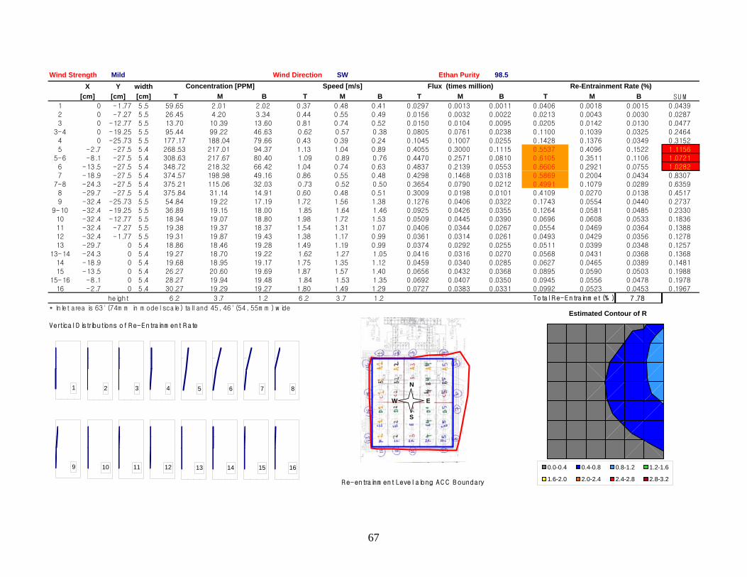
Wind Strength Wind Direction Ethan Purity

0.5537

0.6105

0.66060.5869

0.4991

Mild SW 98.5X Y width

[cm] [cm] [cm] T M B T M B T M B T M B SU M

1 0 -1.77 5.5 59.65 2.01 2.02 0.37 0.48 0.41 0.0297 0.0013 0.0011 0.0406 0.0018 0.0015 0.04392 0 -7.27 5.5 26.45 4.20 3.34 0.44 0.55 0.49 0.0156 0.0032 0.0022 0.0213 0.0043 0.0030 0.0287

3 0 -12.77 5.5 13.70 10.39 13.60 0.81 0.74 0.52 0.0150 0.0104 0.0095 0.0205 0.0142 0.0130 0.0477

3-4 0 -19.25 5.5 95.44 99.22 46.63 0.62 0.57 0.38 0.0805 0.0761 0.0238 0.1100 0.1039 0.0325 0.2464

4 0 -25.73 5.5 177.17 188.04 79.66 0.43 0.39 0.24 0.1045 0.1007 0.0255 0.1428 0.1376 0.0349 0.3152

5 -2.7 -27.5 5.4 268.53 217.01 94.37 1.13 1.04 0.89 0.4055 0.3000 0.1115 0.4096 0.1522 1.1156

5-6 -8.1 -27.5 5.4 308.63 217.67 80.40 1.09 0.89 0.76 0.4470 0.2571 0.0810 0.3511 0.1106 1.0721

6 -13.5 -27.5 5.4 348.72 218.32 66.42 1.04 0.74 0.63 0.4837 0.2139 0.0553 0.2921 0.0755 1.02827 -18.9 -27.5 5.4 374.57 198.98 49.16 0.86 0.55 0.48 0.4298 0.1468 0.0318 0.2004 0.0434 0.8307

7-8 -24.3 -27.5 5.4 375.21 115.06 32.03 0.73 0.52 0.50 0.3654 0.0790 0.0212 0.1079 0.0289 0.6359

8 -29.7 -27.5 5.4 375.84 31.14 14.91 0.60 0.48 0.51 0.3009 0.0198 0.0101 0.4109 0.0270 0.0138 0.4517

9 -32.4 -25.73 5.5 54.84 19.22 17.19 1.72 1.56 1.38 0.1276 0.0406 0.0322 0.1743 0.0554 0.0440 0.2737

9-10 -32.4 -19.25 5.5 36.89 19.15 18.00 1.85 1.64 1.46 0.0925 0.0426 0.0355 0.1264 0.0581 0.0485 0.2330

10 -32.4 -12.77 5.5 18.94 19.07 18.80 1.98 1.72 1.53 0.0509 0.0445 0.0390 0.0696 0.0608 0.0533 0.183611 -32.4 -7.27 5.5 19.38 19.37 18.37 1.54 1.31 1.07 0.0406 0.0344 0.0267 0.0554 0.0469 0.0364 0.1388

12 -32.4 -1.77 5.5 19.31 19.87 19.43 1.38 1.17 0.99 0.0361 0.0314 0.0261 0.0493 0.0429 0.0356 0.1278

13 -29.7 0 5.4 18.86 18.46 19.28 1.49 1.19 0.99 0.0374 0.0292 0.0255 0.0511 0.0399 0.0348 0.1257

13-14 -24.3 0 5.4 19.27 18.70 19.22 1.62 1.27 1.05 0.0416 0.0316 0.0270 0.0568 0.0431 0.0368 0.1368

14 -18.9 0 5.4 19.68 18.95 19.17 1.75 1.35 1.12 0.0459 0.0340 0.0285 0.0627 0.0465 0.0389 0.1481

15 -13.5 0 5.4 26.27 20.60 19.69 1.87 1.57 1.40 0.0656 0.0432 0.0368 0.0895 0.0590 0.0503 0.1988

15-16 -8.1 0 5.4 28.27 19.94 19.48 1.84 1.53 1.35 0.0692 0.0407 0.0350 0.0945 0.0556 0.0478 0.197816 -2.7 0 5.4 30.27 19.29 19.27 1.80 1.49 1.29 0.0727 0.0383 0.0331 0.0992 0.0523 0.0453 0.1967

height 6.2 3.7 1.2 6.2 3.7 1.2 7.78

* Inlet area is 63' (74m m in m odel scale) tall and 45, 46' (54, 55m m ) w ide

Vertical D istributions of R e-Entrainm ent R ate

R e-entrainm ent Level along A C C B oundary

Total R e-Entrainm et (% )

Re-Entrainment Rate (%)Concentration [PPM] Speed [m/s] Flux (times million)

1 2 3 4 5 6 7 8

9 10 11 12 13 14 15 16

N

E

S

W

Estimated Contour of R

0.0-0.4 0.4-0.8 0.8-1.2 1.2-1.6

1.6-2.0 2.0-2.4 2.4-2.8 2.8-3.2

67

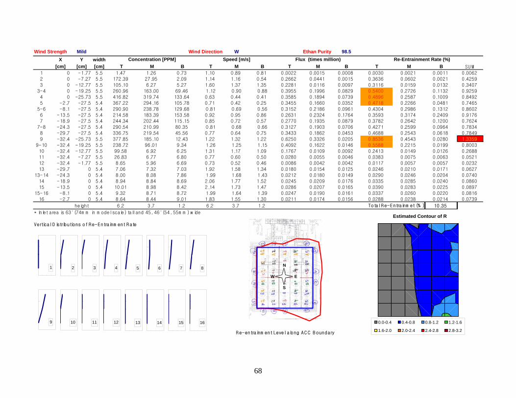
Wind Strength Wind Direction Ethan Purity

0.5400

0.4896

0.4718

0.8536

0.5588

Mild W 98.5X Y width

[cm] [cm] [cm] T M B T M B T M B T M B SU M

1 0 -1.77 5.5 1.47 1.26 0.73 1.10 0.89 0.81 0.0022 0.0015 0.0008 0.0030 0.0021 0.0011 0.00622 0 -7.27 5.5 172.39 27.95 2.09 1.14 1.16 0.54 0.2662 0.0441 0.0015 0.3636 0.0602 0.0021 0.4259

3 0 -12.77 5.5 105.10 6.27 5.27 1.60 1.37 1.35 0.2281 0.0116 0.0097 0.3116 0.0159 0.0132 0.3407

3-4 0 -19.25 5.5 260.96 163.00 69.46 1.12 0.90 0.88 0.3955 0.1996 0.0829 0.2726 0.1132 0.9259

4 0 -25.73 5.5 416.82 319.74 133.64 0.63 0.44 0.41 0.3585 0.1894 0.0739 0.2587 0.1009 0.8492

5 -2.7 -27.5 5.4 367.22 294.16 105.78 0.71 0.42 0.25 0.3455 0.1660 0.0352 0.2266 0.0481 0.7465

5-6 -8.1 -27.5 5.4 290.90 238.78 129.68 0.81 0.69 0.56 0.3152 0.2186 0.0961 0.4304 0.2986 0.1312 0.8602

6 -13.5 -27.5 5.4 214.58 183.39 153.58 0.92 0.95 0.86 0.2631 0.2324 0.1764 0.3593 0.3174 0.2409 0.91767 -18.9 -27.5 5.4 244.34 202.44 115.15 0.85 0.72 0.57 0.2770 0.1935 0.0879 0.3782 0.2642 0.1200 0.7624

7-8 -24.3 -27.5 5.4 290.54 210.99 80.35 0.81 0.68 0.66 0.3127 0.1903 0.0706 0.4271 0.2599 0.0964 0.7834

8 -29.7 -27.5 5.4 336.75 219.54 45.56 0.77 0.64 0.75 0.3433 0.1862 0.0453 0.4688 0.2543 0.0618 0.7849

9 -32.4 -25.73 5.5 377.85 185.10 12.43 1.22 1.32 1.22 0.6250 0.3326 0.0205 0.4543 0.0280 1.3359

9-10 -32.4 -19.25 5.5 238.72 96.01 9.34 1.26 1.25 1.15 0.4092 0.1622 0.0146 0.2215 0.0199 0.8003

10 -32.4 -12.77 5.5 99.58 6.92 6.25 1.31 1.17 1.09 0.1767 0.0109 0.0092 0.2413 0.0149 0.0126 0.268811 -32.4 -7.27 5.5 26.83 6.77 6.80 0.77 0.60 0.50 0.0280 0.0055 0.0046 0.0383 0.0075 0.0063 0.0521

12 -32.4 -1.77 5.5 8.65 5.96 6.69 0.73 0.52 0.46 0.0086 0.0042 0.0042 0.0117 0.0057 0.0057 0.0232

13 -29.7 0 5.4 7.06 7.32 7.03 1.92 1.58 1.34 0.0180 0.0154 0.0125 0.0246 0.0210 0.0171 0.0627

13-14 -24.3 0 5.4 8.00 8.08 7.86 1.99 1.68 1.43 0.0212 0.0180 0.0149 0.0290 0.0246 0.0204 0.0740

14 -18.9 0 5.4 8.94 8.84 8.69 2.06 1.77 1.52 0.0245 0.0209 0.0176 0.0335 0.0285 0.0240 0.0860

15 -13.5 0 5.4 10.01 8.98 8.42 2.14 1.73 1.47 0.0286 0.0207 0.0165 0.0390 0.0283 0.0225 0.0897

15-16 -8.1 0 5.4 9.32 8.71 8.72 1.99 1.64 1.39 0.0247 0.0190 0.0161 0.0337 0.0260 0.0220 0.081616 -2.7 0 5.4 8.64 8.44 9.01 1.83 1.55 1.30 0.0211 0.0174 0.0156 0.0288 0.0238 0.0214 0.0739

height 6.2 3.7 1.2 6.2 3.7 1.2 10.35

* Inlet area is 63' (74m m in m odel scale) tall and 45, 46' (54, 55m m ) w ide

Vertical D istributions of R e-Entrainm ent R ate

R e-entrainm ent Level along A C C B oundary

Total R e-Entrainm et (% )

Re-Entrainment Rate (%)Concentration [PPM] Speed [m/s] Flux (times million)

1 2 3 4 5 6 7 8

9 10 11 12 13 14 15 16

N

E

S

W

Estimated Contour of R

0.0-0.4 0.4-0.8 0.8-1.2 1.2-1.6

1.6-2.0 2.0-2.4 2.4-2.8 2.8-3.2

68

Wind Strength Wind Direction Ethan Purity

1.4287

1.7222

1.8844

0.9111

1.4312

1.4831

Mild N 98.5X Y width

[cm] [cm] [cm] T M B T M B T M B T M B SU M

1 0 -1.77 5.5 1.03 0.60 0.44 1.87 1.62 1.44 0.0026 0.0013 0.0009 0.0036 0.0018 0.0012 0.00662 0 -7.27 5.5 26.48 0.54 0.40 2.13 1.93 0.32 0.0764 0.0014 0.0002 0.1044 0.0019 0.0002 0.1065

3 0 -12.77 5.5 6.79 3.60 3.69 2.27 1.71 0.39 0.0209 0.0084 0.0019 0.0285 0.0114 0.0026 0.0426

3-4 0 -19.25 5.5 6.71 4.88 4.79 1.96 1.50 0.78 0.0179 0.0099 0.0051 0.0244 0.0136 0.0069 0.0449

4 0 -25.73 5.5 6.63 6.15 5.89 1.66 1.29 1.17 0.0149 0.0108 0.0093 0.0204 0.0147 0.0128 0.0479

5 -2.7 -27.5 5.4 12.70 8.16 6.94 1.17 0.76 0.83 0.0197 0.0083 0.0077 0.0270 0.0113 0.0105 0.0488

5-6 -8.1 -27.5 5.4 83.68 8.75 8.40 1.33 0.99 0.93 0.1487 0.0115 0.0104 0.2030 0.0157 0.0142 0.2330

6 -13.5 -27.5 5.4 154.66 9.35 9.87 1.50 1.21 1.03 0.3092 0.0151 0.0136 0.4222 0.0206 0.0185 0.46137 -18.9 -27.5 5.4 445.44 61.72 9.52 1.76 1.67 1.58 1.0462 0.1370 0.0201 0.1871 0.0274 1.6433

7-8 -24.3 -27.5 5.4 612.08 260.86 25.83 1.55 1.58 1.52 1.2611 0.5500 0.0524 0.7511 0.0716 2.5449

8 -29.7 -27.5 5.4 778.72 460.00 42.13 1.33 1.50 1.47 1.3799 0.9185 0.0823 1.2543 0.1124 3.2511

9 -32.4 -25.73 5.5 589.18 526.61 137.26 0.83 0.53 0.77 0.6672 0.3807 0.1438 0.5199 0.1964 1.6274

9-10 -32.4 -19.25 5.5 475.78 421.37 166.88 0.77 0.60 0.62 0.4979 0.3445 0.1403 0.6799 0.4705 0.1917 1.3420

10 -32.4 -12.77 5.5 362.38 316.13 196.49 0.71 0.67 0.47 0.3481 0.2884 0.1246 0.4753 0.3938 0.1702 1.039311 -32.4 -7.27 5.5 338.77 257.52 179.17 0.68 0.57 0.42 0.3138 0.1995 0.1017 0.4285 0.2724 0.1388 0.8397

12 -32.4 -1.77 5.5 474.53 363.77 182.20 0.57 0.74 0.88 0.3650 0.3636 0.2168 0.4984 0.4966 0.2960 1.2910

13 -29.7 0 5.4 574.65 407.55 132.64 1.32 1.43 1.28 1.0095 0.7779 0.2254 1.3786 1.0624 0.3078 2.7488

13-14 -24.3 0 5.4 571.58 348.59 85.91 1.38 1.42 1.26 1.0480 0.6601 0.1446 0.9015 0.1974 2.5301

14 -18.9 0 5.4 568.50 289.63 39.17 1.43 1.41 1.25 1.0860 0.5441 0.0653 0.7431 0.0892 2.3153

15 -13.5 0 5.4 413.27 180.08 18.01 1.34 1.16 0.90 0.7400 0.2793 0.0216 1.0105 0.3815 0.0294 1.4214

15-16 -8.1 0 5.4 217.22 98.92 17.92 1.15 0.88 0.83 0.3334 0.1155 0.0198 0.4553 0.1577 0.0271 0.640216 -2.7 0 5.4 21.17 17.76 17.82 0.96 0.59 0.76 0.0271 0.0139 0.0181 0.0370 0.0190 0.0248 0.0808

height 6.2 3.7 1.2 6.2 3.7 1.2 24.31

* Inlet area is 63' (74m m in m odel scale) tall and 45, 46' (54, 55m m ) w ide

Vertical D istributions of R e-Entrainm ent R ate

R e-entrainm ent Level along A C C B oundary

Total R e-Entrainm et (% )

Re-Entrainment Rate (%)Concentration [PPM] Speed [m/s] Flux (times million)

1 2 3 4 5 6 7 8

9 10 11 12 13 14 15 16

N

E

S

W

Estimated Contour of R

0.0-0.4 0.4-0.8 0.8-1.2 1.2-1.6

1.6-2.0 2.0-2.4 2.4-2.8 2.8-3.2

69

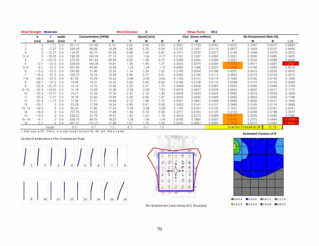
Wind Strength Wind Direction Ethan Purity

0.7539

0.5848

0.4291

0.6190

0.92801.2639

Moderate S 98.5X Y width

[cm] [cm] [cm] T M B T M B T M B T M B SU M

1 0 -1.77 5.5 351.12 141.93 6.10 0.65 0.90 0.63 0.3091 0.1733 0.0052 0.4222 0.2367 0.0072 0.66602 0 -7.27 5.5 228.29 99.68 14.38 0.68 0.76 0.59 0.2107 0.1031 0.0115 0.2877 0.1409 0.0157 0.4442

3 0 -12.77 5.5 116.97 56.75 25.29 0.99 1.00 0.81 0.1571 0.0767 0.0277 0.2146 0.1048 0.0379 0.3572

3-4 0 -19.25 5.5 196.26 109.29 27.13 0.81 1.04 0.77 0.2161 0.1537 0.0282 0.2951 0.2099 0.0385 0.5435

4 0 -25.73 5.5 275.55 161.83 28.96 0.63 1.08 0.72 0.2366 0.2365 0.0284 0.3231 0.3230 0.0388 0.6849

5 -2.7 -27.5 5.4 328.59 169.36 16.81 1.26 1.45 1.27 0.5520 0.3274 0.0284 0.4471 0.0387 1.2397

5-6 -8.1 -27.5 5.4 267.69 95.66 14.58 1.20 1.24 1.15 0.4282 0.1586 0.0222 0.2166 0.0304 0.8318

6 -13.5 -27.5 5.4 206.80 21.96 12.35 1.14 1.04 1.02 0.3142 0.0304 0.0168 0.0415 0.0230 0.49357 -18.9 -27.5 5.4 159.72 16.16 14.49 0.98 0.72 0.61 0.2082 0.0156 0.0117 0.2843 0.0213 0.0159 0.3215

7-8 -24.3 -27.5 5.4 87.33 15.24 14.25 0.98 0.69 0.60 0.1143 0.0141 0.0114 0.1560 0.0192 0.0156 0.1908

8 -29.7 -27.5 5.4 14.93 14.31 14.02 0.99 0.66 0.60 0.0196 0.0126 0.0112 0.0268 0.0172 0.0153 0.0593

9 -32.4 -25.73 5.5 15.14 15.70 15.45 2.23 2.01 1.73 0.0458 0.0428 0.0362 0.0625 0.0585 0.0494 0.1704

9-10 -32.4 -19.25 5.5 15.18 15.56 15.38 2.32 2.09 1.81 0.0479 0.0441 0.0378 0.0654 0.0602 0.0517 0.1772

10 -32.4 -12.77 5.5 15.21 15.43 15.30 2.42 2.16 1.90 0.0500 0.0453 0.0395 0.0682 0.0619 0.0539 0.184011 -32.4 -7.27 5.5 16.16 15.60 14.89 2.28 2.09 1.81 0.0500 0.0442 0.0366 0.0683 0.0603 0.0500 0.1786

12 -32.4 -1.77 5.5 17.36 17.21 16.90 2.13 1.98 1.70 0.0501 0.0461 0.0389 0.0685 0.0630 0.0531 0.1846

13 -29.7 0 5.4 33.28 17.28 16.54 0.80 0.61 0.58 0.0353 0.0141 0.0127 0.0482 0.0193 0.0174 0.0849

13-14 -24.3 0 5.4 95.52 17.80 17.20 0.94 0.68 0.58 0.1195 0.0161 0.0132 0.1631 0.0220 0.0181 0.2031

14 -18.9 0 5.4 157.76 18.33 17.86 1.08 0.74 0.58 0.2271 0.0181 0.0137 0.3102 0.0248 0.0188 0.3537

15 -13.5 0 5.4 238.22 22.79 18.47 1.43 1.23 1.18 0.4533 0.0373 0.0289 0.0509 0.0395 0.7094

15-16 -8.1 0 5.4 339.79 96.76 18.23 1.50 1.46 1.34 0.6795 0.1885 0.0325 0.2575 0.0444 1.229916 -2.7 0 5.4 441.37 170.73 17.98 1.57 1.70 1.50 0.9255 0.3861 0.0360 0.5272 0.0492 1.8403

height 6.2 3.7 1.2 6.2 3.7 1.2 11.15

* Inlet area is 63' (74m m in m odel scale) tall and 45, 46' (54, 55m m ) w ide

Vertical D istributions of R e-Entrainm ent R ate

R e-entrainm ent Level along A C C B oundary

Total R e-Entrainm et (% )

Re-Entrainment Rate (%)Concentration [PPM] Speed [m/s] Flux (times million)

1 2 3 4 5 6 7 8

9 10 11 12 13 14 15 16

N

E

S

W

Estimated Contour of R

0.0-0.4 0.4-0.8 0.8-1.2 1.2-1.6

1.6-2.0 2.0-2.4 2.4-2.8 2.8-3.2

70

Wind Strength Wind Direction Ethan Purity

0.4734 0.3567

0.2696

0.1128

0.2837

0.4423

0.0767

Moderate SW 98.5X Y width

[cm] [cm] [cm] T M B T M B T M B T M B SU M

1 0 -1.77 5.5 27.68 0.49 0.94 0.63 0.67 0.47 0.0236 0.0004 0.0006 0.0322 0.0006 0.0008 0.03372 0 -7.27 5.5 14.38 3.09 3.19 0.75 0.69 0.48 0.0146 0.0029 0.0021 0.0199 0.0039 0.0028 0.0267

3 0 -12.77 5.5 37.04 6.33 6.88 0.81 1.13 0.75 0.0405 0.0097 0.0070 0.0553 0.0133 0.0096 0.0782

3-4 0 -19.25 5.5 101.34 76.18 60.35 0.65 0.88 0.63 0.0889 0.0914 0.0516 0.1214 0.1248 0.0705 0.3168

4 0 -25.73 5.5 165.63 146.03 113.81 0.49 0.64 0.51 0.1096 0.1262 0.0787 0.1496 0.1723 0.1075 0.4294

5 -2.7 -27.5 5.4 232.50 184.86 101.47 1.12 1.06 0.93 0.3466 0.2612 0.1257 0.1716 1.0017

5-6 -8.1 -27.5 5.4 155.85 113.03 58.95 0.95 0.77 0.79 0.1974 0.1153 0.0620 0.1574 0.0847 0.5118

6 -13.5 -27.5 5.4 79.19 41.21 16.42 0.78 0.47 0.65 0.0826 0.0258 0.0142 0.0353 0.0194 0.16757 -18.9 -27.5 5.4 116.45 72.06 13.78 0.67 0.80 0.80 0.1041 0.0770 0.0146 0.1422 0.1052 0.0200 0.2674

7-8 -24.3 -27.5 5.4 217.12 43.12 12.68 0.72 0.90 0.92 0.2077 0.0516 0.0155 0.0705 0.0211 0.3753

8 -29.7 -27.5 5.4 317.79 14.18 11.58 0.77 1.00 1.04 0.3239 0.0188 0.0160 0.0257 0.0218 0.4898

9 -32.4 -25.73 5.5 19.87 11.45 12.04 2.08 1.94 1.71 0.0562 0.0302 0.0280 0.0412 0.0382 0.1561

9-10 -32.4 -19.25 5.5 16.11 11.56 11.66 2.14 1.94 1.71 0.0469 0.0305 0.0270 0.0640 0.0416 0.0368 0.1425

10 -32.4 -12.77 5.5 12.35 11.67 11.28 2.21 1.94 1.70 0.0369 0.0308 0.0260 0.0504 0.0420 0.0355 0.128011 -32.4 -7.27 5.5 12.73 11.08 12.15 1.66 1.48 1.18 0.0287 0.0222 0.0195 0.0392 0.0303 0.0266 0.0960

12 -32.4 -1.77 5.5 11.71 11.54 11.73 1.67 1.41 1.19 0.0265 0.0221 0.0189 0.0362 0.0302 0.0258 0.0922

13 -29.7 0 5.4 13.19 13.16 12.59 1.81 1.45 1.21 0.0317 0.0254 0.0202 0.0433 0.0347 0.0276 0.1056

13-14 -24.3 0 5.4 15.62 13.57 12.43 1.85 1.45 1.20 0.0385 0.0262 0.0198 0.0525 0.0358 0.0271 0.1154

14 -18.9 0 5.4 18.05 13.98 12.27 1.89 1.45 1.19 0.0455 0.0270 0.0194 0.0621 0.0369 0.0265 0.1255

15 -13.5 0 5.4 27.30 14.73 13.33 2.10 1.84 1.65 0.0762 0.0362 0.0294 0.1041 0.0494 0.0401 0.1936

15-16 -8.1 0 5.4 22.26 14.29 14.05 2.16 1.88 1.66 0.0640 0.0357 0.0311 0.0875 0.0488 0.0425 0.178716 -2.7 0 5.4 17.23 13.85 14.76 2.22 1.91 1.67 0.0510 0.0353 0.0328 0.0697 0.0482 0.0448 0.1627

height 6.2 3.7 1.2 6.2 3.7 1.2 5.19

* Inlet area is 63' (74m m in m odel scale) tall and 45, 46' (54, 55m m ) w ide

Vertical D istributions of R e-Entrainm ent R ate

R e-entrainm ent Level along A C C B oundary

Total R e-Entrainm et (% )

Re-Entrainment Rate (%)Concentration [PPM] Speed [m/s] Flux (times million)

1 2 3 4 5 6 7 8

9 10 11 12 13 14 15 16

N

E

S

W

Estimated Contour of R

0.0-0.4 0.4-0.8 0.8-1.2 1.2-1.6

1.6-2.0 2.0-2.4 2.4-2.8 2.8-3.2

71

Wind Strength Wind Direction Ethan Purity

0.6419

0.6776

0.6015

0.5750

0.6027

Moderate W 98.5X Y width

[cm] [cm] [cm] T M B T M B T M B T M B SU M

1 0 -1.77 5.5 4.50 1.08 1.12 1.16 1.05 0.95 0.0071 0.0015 0.0014 0.0097 0.0021 0.0020 0.01382 0 -7.27 5.5 77.96 12.02 3.98 1.07 0.88 0.96 0.1131 0.0143 0.0052 0.1544 0.0195 0.0071 0.1810

3 0 -12.77 5.5 158.35 169.39 7.06 1.54 1.53 1.70 0.3302 0.3526 0.0162 0.4509 0.4815 0.0222 0.9546

3-4 0 -19.25 5.5 286.40 177.01 19.06 1.21 1.07 1.06 0.4700 0.2581 0.0273 0.3525 0.0373 1.0317

4 0 -25.73 5.5 414.45 184.63 31.06 0.88 0.62 0.42 0.4962 0.1541 0.0176 0.2105 0.0241 0.9121

5 -2.7 -27.5 5.4 282.01 189.15 105.96 0.54 0.53 0.36 0.2018 0.1340 0.0505 0.2756 0.1830 0.0690 0.5276

5-6 -8.1 -27.5 5.4 273.04 187.15 124.58 0.69 0.62 0.50 0.2498 0.1535 0.0822 0.3411 0.2097 0.1123 0.6630

6 -13.5 -27.5 5.4 264.07 185.15 143.20 0.84 0.70 0.63 0.2941 0.1726 0.1207 0.4017 0.2357 0.1649 0.80237 -18.9 -27.5 5.4 318.99 245.18 77.20 1.04 0.89 0.69 0.4404 0.2911 0.0713 0.3975 0.0973 1.0964

7-8 -24.3 -27.5 5.4 359.51 210.07 50.22 0.88 0.96 0.99 0.4211 0.2684 0.0663 0.3665 0.0905 1.0320

8 -29.7 -27.5 5.4 400.03 174.96 23.24 0.72 1.03 1.29 0.3847 0.2393 0.0399 0.5253 0.3267 0.0545 0.9066

9 -32.4 -25.73 5.5 261.42 92.22 17.72 1.24 1.40 1.29 0.4413 0.1746 0.0311 0.2385 0.0424 0.8836

9-10 -32.4 -19.25 5.5 158.43 55.53 18.41 1.10 1.12 1.05 0.2371 0.0845 0.0262 0.3238 0.1153 0.0358 0.4749

10 -32.4 -12.77 5.5 55.44 18.83 19.11 0.96 0.85 0.80 0.0723 0.0216 0.0209 0.0988 0.0295 0.0285 0.156811 -32.4 -7.27 5.5 46.04 17.76 18.62 0.62 0.63 0.63 0.0387 0.0152 0.0160 0.0528 0.0208 0.0218 0.0954

12 -32.4 -1.77 5.5 27.19 20.71 19.58 0.68 0.60 0.60 0.0252 0.0169 0.0159 0.0345 0.0231 0.0217 0.0792

13 -29.7 0 5.4 21.14 21.34 20.78 2.25 1.96 1.60 0.0635 0.0557 0.0444 0.0867 0.0761 0.0606 0.2234

13-14 -24.3 0 5.4 21.88 21.95 21.56 2.28 2.00 1.66 0.0666 0.0585 0.0476 0.0909 0.0799 0.0650 0.2358

14 -18.9 0 5.4 22.62 22.57 22.34 2.31 2.04 1.71 0.0697 0.0613 0.0509 0.0952 0.0837 0.0695 0.2485

15 -13.5 0 5.4 22.53 22.31 23.25 2.27 2.01 1.68 0.0680 0.0597 0.0521 0.0929 0.0815 0.0711 0.2455

15-16 -8.1 0 5.4 22.54 23.27 23.56 2.21 1.96 1.60 0.0663 0.0607 0.0504 0.0905 0.0829 0.0688 0.242216 -2.7 0 5.4 22.54 24.23 23.87 2.15 1.91 1.53 0.0646 0.0617 0.0486 0.0882 0.0842 0.0664 0.2387

height 6.2 3.7 1.2 6.2 3.7 1.2 11.25

* Inlet area is 63' (74m m in m odel scale) tall and 45, 46' (54, 55m m ) w ide

Vertical D istributions of R e-Entrainm ent R ate

R e-entrainm ent Level along A C C B oundary

Total R e-Entrainm et (% )

Re-Entrainment Rate (%)Concentration [PPM] Speed [m/s] Flux (times million)

1 2 3 4 5 6 7 8

9 10 11 12 13 14 15 16

N

E

S

W

Estimated Contour of R

0.0-0.4 0.4-0.8 0.8-1.2 1.2-1.6

1.6-2.0 2.0-2.4 2.4-2.8 2.8-3.2

72

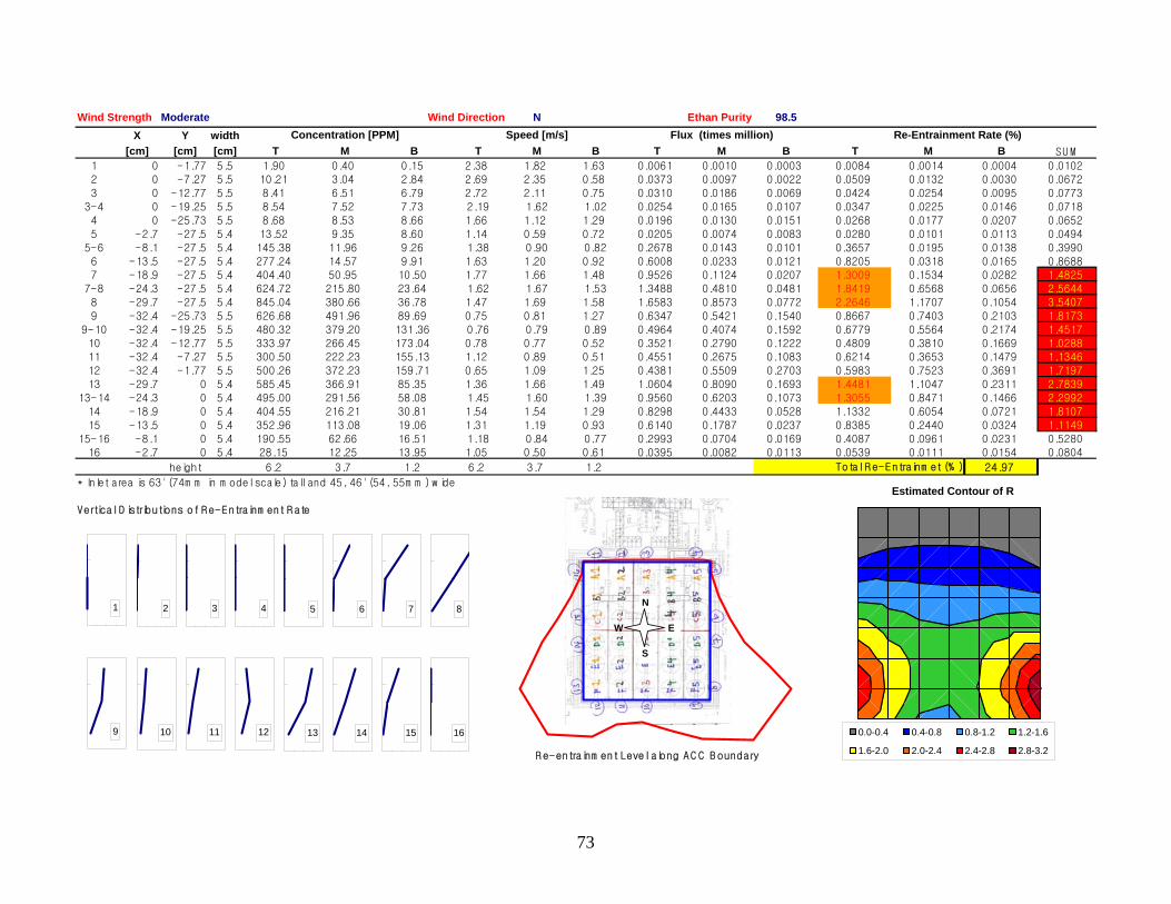
Wind Strength Wind Direction Ethan Purity

1.3009

1.8419

2.2646

0.8667

1.4481

1.3055

Moderate N 98.5X Y width

[cm] [cm] [cm] T M B T M B T M B T M B SU M

1 0 -1.77 5.5 1.90 0.40 0.15 2.38 1.82 1.63 0.0061 0.0010 0.0003 0.0084 0.0014 0.0004 0.01022 0 -7.27 5.5 10.21 3.04 2.84 2.69 2.35 0.58 0.0373 0.0097 0.0022 0.0509 0.0132 0.0030 0.0672

3 0 -12.77 5.5 8.41 6.51 6.79 2.72 2.11 0.75 0.0310 0.0186 0.0069 0.0424 0.0254 0.0095 0.0773

3-4 0 -19.25 5.5 8.54 7.52 7.73 2.19 1.62 1.02 0.0254 0.0165 0.0107 0.0347 0.0225 0.0146 0.0718

4 0 -25.73 5.5 8.68 8.53 8.66 1.66 1.12 1.29 0.0196 0.0130 0.0151 0.0268 0.0177 0.0207 0.0652

5 -2.7 -27.5 5.4 13.52 9.35 8.60 1.14 0.59 0.72 0.0205 0.0074 0.0083 0.0280 0.0101 0.0113 0.0494

5-6 -8.1 -27.5 5.4 145.38 11.96 9.26 1.38 0.90 0.82 0.2678 0.0143 0.0101 0.3657 0.0195 0.0138 0.3990

6 -13.5 -27.5 5.4 277.24 14.57 9.91 1.63 1.20 0.92 0.6008 0.0233 0.0121 0.8205 0.0318 0.0165 0.86887 -18.9 -27.5 5.4 404.40 50.95 10.50 1.77 1.66 1.48 0.9526 0.1124 0.0207 0.1534 0.0282 1.4825

7-8 -24.3 -27.5 5.4 624.72 215.80 23.64 1.62 1.67 1.53 1.3488 0.4810 0.0481 0.6568 0.0656 2.5644

8 -29.7 -27.5 5.4 845.04 380.66 36.78 1.47 1.69 1.58 1.6583 0.8573 0.0772 1.1707 0.1054 3.5407

9 -32.4 -25.73 5.5 626.68 491.96 89.69 0.75 0.81 1.27 0.6347 0.5421 0.1540 0.7403 0.2103 1.8173

9-10 -32.4 -19.25 5.5 480.32 379.20 131.36 0.76 0.79 0.89 0.4964 0.4074 0.1592 0.6779 0.5564 0.2174 1.4517

10 -32.4 -12.77 5.5 333.97 266.45 173.04 0.78 0.77 0.52 0.3521 0.2790 0.1222 0.4809 0.3810 0.1669 1.028811 -32.4 -7.27 5.5 300.50 222.23 155.13 1.12 0.89 0.51 0.4551 0.2675 0.1083 0.6214 0.3653 0.1479 1.1346

12 -32.4 -1.77 5.5 500.26 372.23 159.71 0.65 1.09 1.25 0.4381 0.5509 0.2703 0.5983 0.7523 0.3691 1.7197

13 -29.7 0 5.4 585.45 366.91 85.35 1.36 1.66 1.49 1.0604 0.8090 0.1693 1.1047 0.2311 2.7839

13-14 -24.3 0 5.4 495.00 291.56 58.08 1.45 1.60 1.39 0.9560 0.6203 0.1073 0.8471 0.1466 2.2992

14 -18.9 0 5.4 404.55 216.21 30.81 1.54 1.54 1.29 0.8298 0.4433 0.0528 1.1332 0.6054 0.0721 1.8107

15 -13.5 0 5.4 352.96 113.08 19.06 1.31 1.19 0.93 0.6140 0.1787 0.0237 0.8385 0.2440 0.0324 1.1149

15-16 -8.1 0 5.4 190.55 62.66 16.51 1.18 0.84 0.77 0.2993 0.0704 0.0169 0.4087 0.0961 0.0231 0.528016 -2.7 0 5.4 28.15 12.25 13.95 1.05 0.50 0.61 0.0395 0.0082 0.0113 0.0539 0.0111 0.0154 0.0804

height 6.2 3.7 1.2 6.2 3.7 1.2 24.97

* Inlet area is 63' (74m m in m odel scale) tall and 45, 46' (54, 55m m ) w ide

Vertical D istributions of R e-Entrainm ent R ate

R e-entrainm ent Level along A C C B oundary

Total R e-Entrainm et (% )

Re-Entrainment Rate (%)Concentration [PPM] Speed [m/s] Flux (times million)

1 2 3 4 5 6 7 8

9 10 11 12 13 14 15 16

N

E

S

W

Estimated Contour of R

0.0-0.4 0.4-0.8 0.8-1.2 1.2-1.6

1.6-2.0 2.0-2.4 2.4-2.8 2.8-3.2

73

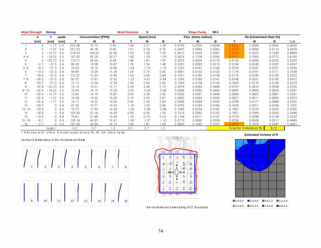
Wind Strength Wind Direction Ethan Purity

0.64590.4707

0.5205

0.5017

0.6624

Strong S 98.5X Y width

[cm] [cm] [cm] T M B T M B T M B T M B SU M

1 0 -1.77 5.5 223.38 70.13 2.45 1.56 2.31 1.39 0.4730 0.2203 0.0046 0.3008 0.0063 0.95302 0 -7.27 5.5 251.53 45.18 8.05 1.01 0.79 0.75 0.3447 0.0482 0.0082 0.0658 0.0113 0.5478

3 0 -12.77 5.5 218.34 140.02 52.06 1.29 1.28 1.39 0.3812 0.2434 0.0981 0.3323 0.1340 0.9869

3-4 0 -19.25 5.5 167.02 82.29 30.77 1.62 1.55 1.35 0.3674 0.1728 0.0566 0.2360 0.0772 0.8149

4 0 -25.73 5.5 115.71 24.55 9.49 1.96 1.81 1.32 0.3070 0.0605 0.0170 0.4193 0.0826 0.0232 0.5250

5 -2.7 -27.5 5.4 99.20 19.08 10.67 1.76 1.54 1.48 0.2331 0.0393 0.0210 0.3184 0.0536 0.0287 0.4007

5-6 -8.1 -27.5 5.4 74.50 16.19 10.96 1.53 1.15 1.16 0.1520 0.0247 0.0169 0.2076 0.0337 0.0231 0.2643

6 -13.5 -27.5 5.4 49.80 13.29 11.26 1.30 0.75 0.83 0.0861 0.0132 0.0125 0.1176 0.0181 0.0171 0.15287 -18.9 -27.5 5.4 112.57 15.22 12.45 1.03 0.89 0.84 0.1551 0.0180 0.0139 0.2118 0.0245 0.0190 0.2553

7-8 -24.3 -27.5 5.4 92.37 13.91 12.52 1.22 0.91 0.84 0.1500 0.0169 0.0141 0.2048 0.0231 0.0192 0.2472

8 -29.7 -27.5 5.4 72.17 12.59 12.58 1.40 0.94 0.85 0.1350 0.0158 0.0142 0.1843 0.0216 0.0194 0.2253

9 -32.4 -25.73 5.5 13.15 14.21 12.71 3.24 3.08 2.70 0.0579 0.0593 0.0466 0.0791 0.0810 0.0636 0.2236

9-10 -32.4 -19.25 5.5 13.40 14.15 13.29 3.22 3.08 2.68 0.0586 0.0592 0.0482 0.0800 0.0809 0.0659 0.2267

10 -32.4 -12.77 5.5 13.65 14.10 13.87 3.20 3.09 2.65 0.0592 0.0591 0.0499 0.0808 0.0807 0.0681 0.229711 -32.4 -7.27 5.5 14.28 14.35 14.26 3.10 3.05 2.61 0.0602 0.0594 0.0506 0.0821 0.0811 0.0690 0.2323

12 -32.4 -1.77 5.5 14.11 14.22 14.04 3.05 2.95 2.64 0.0585 0.0569 0.0502 0.0798 0.0777 0.0686 0.2262

13 -29.7 0 5.4 47.50 13.71 14.25 1.19 1.00 0.96 0.0752 0.0183 0.0182 0.1026 0.0251 0.0248 0.1525

13-14 -24.3 0 5.4 76.72 17.93 14.34 1.06 0.98 0.98 0.1085 0.0234 0.0187 0.1481 0.0319 0.0255 0.2056

14 -18.9 0 5.4 105.95 22.16 14.43 0.93 0.95 1.00 0.1319 0.0282 0.0192 0.1801 0.0384 0.0262 0.2448

15 -13.5 0 5.4 74.81 21.96 15.09 1.16 0.74 0.53 0.1156 0.0217 0.0107 0.1579 0.0296 0.0146 0.2022

15-16 -8.1 0 5.4 133.18 40.97 15.61 1.53 1.27 1.10 0.2715 0.0695 0.0228 0.3708 0.0949 0.0311 0.496916 -2.7 0 5.4 191.56 59.99 16.14 1.90 1.81 1.66 0.4850 0.1442 0.0357 0.1970 0.0487 0.9081

height 6.2 3.7 1.2 6.2 3.7 1.2 8.72

* Inlet area is 63' (74m m in m odel scale) tall and 45, 46' (54, 55m m ) w ide

Vertical D istributions of R e-Entrainm ent R ate

R e-entrainm ent Level along A C C B oundary

Total R e-Entrainm et (% )

Re-Entrainment Rate (%)Concentration [PPM] Speed [m/s] Flux (times million)

1 2 3 4 5 6 7 8

9 10 11 12 13 14 15 16

N

E

S

W

Estimated Contour of R

0.0-0.4 0.4-0.8 0.8-1.2 1.2-1.6

1.6-2.0 2.0-2.4 2.4-2.8 2.8-3.2

74

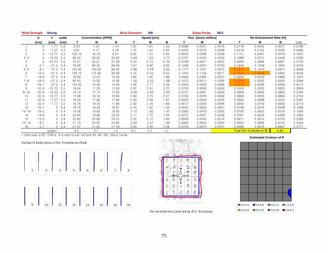
Wind Strength Wind Direction Ethan Purity

0.1607

0.1643 0.1548

0.2284

0.3318

0.1024

Strong SW 98.5X Y width

[cm] [cm] [cm] T M B T M B T M B T M B SU M

1 0 -1.77 5.5 3.93 1.25 1.14 1.62 1.81 1.26 0.0086 0.0031 0.0019 0.0118 0.0042 0.0027 0.01862 0 -7.27 5.5 9.81 4.17 3.78 1.75 1.32 0.93 0.0233 0.0075 0.0048 0.0318 0.0102 0.0065 0.0485

3 0 -12.77 5.5 100.13 16.73 6.57 0.62 1.31 0.65 0.0843 0.0298 0.0058 0.1151 0.0407 0.0079 0.1637

3-4 0 -19.25 5.5 86.20 39.62 33.82 0.68 1.02 0.72 0.0797 0.0550 0.0329 0.1088 0.0751 0.0449 0.2289

4 0 -25.73 5.5 72.27 62.51 61.08 0.74 0.73 0.79 0.0728 0.0621 0.0652 0.0994 0.0848 0.0891 0.2732

5 -2.7 -27.5 5.4 78.66 84.32 84.43 1.01 0.82 0.65 0.1058 0.0922 0.0733 0.1444 0.1259 0.1000 0.3704

5-6 -8.1 -27.5 5.4 102.40 100.00 84.45 0.86 0.78 0.60 0.1177 0.1037 0.0675 0.1416 0.0921 0.3944

6 -13.5 -27.5 5.4 126.15 115.69 84.48 0.72 0.74 0.55 0.1203 0.1134 0.0617 0.0842 0.40347 -18.9 -27.5 5.4 18.09 15.02 14.28 1.84 1.92 1.88 0.0444 0.0385 0.0357 0.0606 0.0526 0.0488 0.1620

7-8 -24.3 -27.5 5.4 80.55 15.30 14.96 1.56 2.02 1.98 0.1672 0.0411 0.0395 0.0562 0.0540 0.3386

8 -29.7 -27.5 5.4 143.00 15.59 15.64 1.28 2.11 2.09 0.2430 0.0439 0.0436 0.0599 0.0595 0.4512

9 -32.4 -25.73 5.5 18.59 17.28 17.06 2.97 2.91 2.70 0.0750 0.0683 0.0624 0.0933 0.0853 0.2809

9-10 -32.4 -19.25 5.5 18.14 17.73 17.83 2.96 2.83 2.60 0.0727 0.0681 0.0630 0.0993 0.0930 0.0860 0.2784

10 -32.4 -12.77 5.5 17.68 18.19 18.60 2.94 2.75 2.51 0.0705 0.0678 0.0634 0.0963 0.0926 0.0866 0.275411 -32.4 -7.27 5.5 19.54 17.89 17.86 2.34 2.08 1.67 0.0620 0.0504 0.0405 0.0846 0.0688 0.0553 0.2087

12 -32.4 -1.77 5.5 19.78 18.76 17.89 2.30 2.18 1.84 0.0617 0.0555 0.0446 0.0843 0.0759 0.0609 0.2210

13 -29.7 0 5.4 18.76 19.34 18.91 2.19 1.92 1.59 0.0547 0.0493 0.0401 0.0748 0.0674 0.0548 0.1969

13-14 -24.3 0 5.4 19.58 19.65 19.45 2.15 1.82 1.47 0.0560 0.0476 0.0380 0.0765 0.0650 0.0519 0.1934

14 -18.9 0 5.4 20.40 19.96 20.00 2.11 1.72 1.34 0.0572 0.0457 0.0358 0.0781 0.0624 0.0488 0.1894

15 -13.5 0 5.4 20.82 20.89 20.31 2.30 2.13 1.90 0.0638 0.0593 0.0514 0.0871 0.0810 0.0703 0.2383

15-16 -8.1 0 5.4 21.19 20.97 20.80 2.42 2.27 1.99 0.0683 0.0633 0.0552 0.0932 0.0864 0.0754 0.255016 -2.7 0 5.4 21.57 21.05 21.29 2.54 2.40 2.08 0.0729 0.0673 0.0591 0.0996 0.0919 0.0807 0.2721

height 6.2 3.7 1.2 6.2 3.7 1.2 5.46

* Inlet area is 63' (74m m in m odel scale) tall and 45, 46' (54, 55m m ) w ide

Vertical D istributions of R e-Entrainm ent R ate

R e-entrainm ent Level along A C C B oundary

Total R e-Entrainm et (% )

Re-Entrainment Rate (%)Concentration [PPM] Speed [m/s] Flux (times million)

1 2 3 4 5 6 7 8

9 10 11 12 13 14 15 16

N

E

S

W

Estimated Contour of R

0.0-0.4 0.4-0.8 0.8-1.2 1.2-1.6

1.6-2.0 2.0-2.4 2.4-2.8 2.8-3.2

75

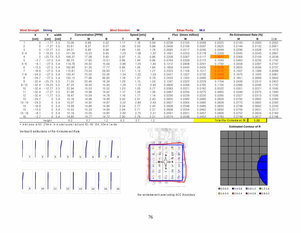
Wind Strength Wind Direction Ethan Purity

0.3015

0.25380.3172

0.3306

0.3323

0.1704

Strong W 98.5X Y width

[cm] [cm] [cm] T M B T M B T M B T M B SU M

1 0 -1.77 5.5 15.06 6.68 5.32 1.17 1.16 0.94 0.0238 0.0105 0.0068 0.0325 0.0143 0.0093 0.05622 0 -7.27 5.5 33.61 8.37 8.07 1.00 0.93 0.88 0.0458 0.0106 0.0097 0.0625 0.0144 0.0132 0.0901

3 0 -12.77 5.5 34.31 9.99 9.96 1.49 1.60 1.78 0.0695 0.0217 0.0240 0.0949 0.0296 0.0328 0.1573

3-4 0 -19.25 5.5 101.34 13.53 9.95 1.23 1.38 1.32 0.1691 0.0253 0.0178 0.2309 0.0345 0.0243 0.2897

4 0 -25.73 5.5 168.37 17.08 9.95 0.97 1.15 0.86 0.2208 0.0267 0.0117 0.0364 0.0159 0.3538

5 -2.7 -27.5 5.4 66.73 17.65 13.51 0.86 1.44 0.96 0.0764 0.0339 0.0172 0.1043 0.0463 0.0235 0.1742

5-6 -8.1 -27.5 5.4 114.76 24.50 15.64 0.86 1.25 1.40 0.1312 0.0408 0.0291 0.1792 0.0558 0.0397 0.2747

6 -13.5 -27.5 5.4 162.80 31.35 17.77 0.86 1.06 1.84 0.1859 0.0443 0.0435 0.0605 0.0594 0.37377 -18.9 -27.5 5.4 115.81 73.03 59.93 1.51 1.13 1.27 0.2323 0.1104 0.1017 0.1507 0.1389 0.6068

7-8 -24.3 -27.5 5.4 135.47 75.50 53.26 1.34 1.22 1.03 0.2421 0.1227 0.0732 0.1675 0.1000 0.5981

8 -29.7 -27.5 5.4 155.12 77.96 46.60 1.18 1.31 0.79 0.2433 0.1355 0.0490 0.1851 0.0669 0.5843

9 -32.4 -25.73 5.5 71.55 20.46 16.34 1.29 1.15 1.03 0.1247 0.0320 0.0229 0.0436 0.0312 0.2452

9-10 -32.4 -19.25 5.5 47.24 18.00 15.93 1.26 1.10 0.90 0.0806 0.0268 0.0195 0.1100 0.0366 0.0266 0.1732

10 -32.4 -12.77 5.5 22.94 15.53 15.52 1.23 1.05 0.77 0.0383 0.0221 0.0162 0.0522 0.0301 0.0221 0.104511 -32.4 -7.27 5.5 31.96 14.98 14.92 1.12 1.26 1.36 0.0487 0.0256 0.0275 0.0665 0.0349 0.0375 0.1390

12 -32.4 -1.77 5.5 18.47 15.09 14.78 1.16 1.17 1.14 0.0290 0.0239 0.0230 0.0395 0.0327 0.0313 0.1036

13 -29.7 0 5.4 15.16 14.98 14.99 3.00 2.91 2.43 0.0605 0.0580 0.0485 0.0826 0.0792 0.0662 0.2280

13-14 -24.3 0 5.4 15.07 14.92 14.97 3.02 2.84 2.43 0.0607 0.0564 0.0485 0.0828 0.0770 0.0662 0.2260

14 -18.9 0 5.4 14.99 14.86 14.96 3.04 2.77 2.43 0.0608 0.0548 0.0485 0.0830 0.0748 0.0662 0.2240

15 -13.5 0 5.4 15.53 15.33 14.99 2.94 2.71 2.31 0.0608 0.0554 0.0462 0.0830 0.0756 0.0631 0.2217

15-16 -8.1 0 5.4 15.19 15.05 14.85 2.92 2.75 2.31 0.0591 0.0551 0.0457 0.0806 0.0752 0.0624 0.218316 -2.7 0 5.4 14.85 14.77 14.72 2.90 2.78 2.31 0.0574 0.0548 0.0452 0.0783 0.0748 0.0617 0.2148

height 6.2 3.7 1.2 6.2 3.7 1.2 5.66

* Inlet area is 63' (74m m in m odel scale) tall and 45, 46' (54, 55m m ) w ide

Vertical D istributions of R e-Entrainm ent R ate

R e-entrainm ent Level along A C C B oundary

Total R e-Entrainm et (% )

Re-Entrainment Rate (%)Concentration [PPM] Speed [m/s] Flux (times million)

1 2 3 4 5 6 7 8

9 10 11 12 13 14 15 16

N

E

S

W

Estimated Contour of R

0.0-0.4 0.4-0.8 0.8-1.2 1.2-1.6

1.6-2.0 2.0-2.4 2.4-2.8 2.8-3.2

76

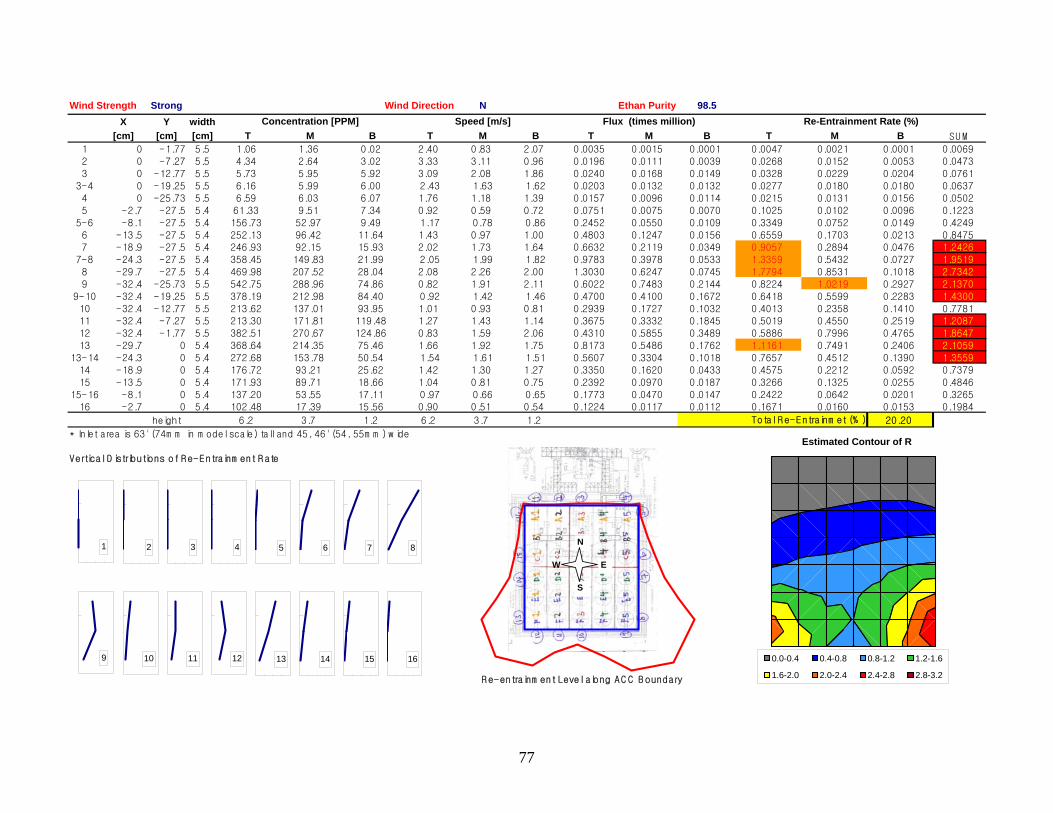
Wind Strength Wind Direction Ethan Purity

0.9057

1.3359

1.7794

0.8224 1.0219

1.1161

Strong N 98.5X Y width

[cm] [cm] [cm] T M B T M B T M B T M B SU M

1 0 -1.77 5.5 1.06 1.36 0.02 2.40 0.83 2.07 0.0035 0.0015 0.0001 0.0047 0.0021 0.0001 0.00692 0 -7.27 5.5 4.34 2.64 3.02 3.33 3.11 0.96 0.0196 0.0111 0.0039 0.0268 0.0152 0.0053 0.0473

3 0 -12.77 5.5 5.73 5.95 5.92 3.09 2.08 1.86 0.0240 0.0168 0.0149 0.0328 0.0229 0.0204 0.0761

3-4 0 -19.25 5.5 6.16 5.99 6.00 2.43 1.63 1.62 0.0203 0.0132 0.0132 0.0277 0.0180 0.0180 0.0637

4 0 -25.73 5.5 6.59 6.03 6.07 1.76 1.18 1.39 0.0157 0.0096 0.0114 0.0215 0.0131 0.0156 0.0502

5 -2.7 -27.5 5.4 61.33 9.51 7.34 0.92 0.59 0.72 0.0751 0.0075 0.0070 0.1025 0.0102 0.0096 0.1223

5-6 -8.1 -27.5 5.4 156.73 52.97 9.49 1.17 0.78 0.86 0.2452 0.0550 0.0109 0.3349 0.0752 0.0149 0.4249

6 -13.5 -27.5 5.4 252.13 96.42 11.64 1.43 0.97 1.00 0.4803 0.1247 0.0156 0.6559 0.1703 0.0213 0.84757 -18.9 -27.5 5.4 246.93 92.15 15.93 2.02 1.73 1.64 0.6632 0.2119 0.0349 0.2894 0.0476 1.2426

7-8 -24.3 -27.5 5.4 358.45 149.83 21.99 2.05 1.99 1.82 0.9783 0.3978 0.0533 0.5432 0.0727 1.9519

8 -29.7 -27.5 5.4 469.98 207.52 28.04 2.08 2.26 2.00 1.3030 0.6247 0.0745 0.8531 0.1018 2.7342

9 -32.4 -25.73 5.5 542.75 288.96 74.86 0.82 1.91 2.11 0.6022 0.7483 0.2144 0.2927 2.1370

9-10 -32.4 -19.25 5.5 378.19 212.98 84.40 0.92 1.42 1.46 0.4700 0.4100 0.1672 0.6418 0.5599 0.2283 1.4300

10 -32.4 -12.77 5.5 213.62 137.01 93.95 1.01 0.93 0.81 0.2939 0.1727 0.1032 0.4013 0.2358 0.1410 0.778111 -32.4 -7.27 5.5 213.30 171.81 119.48 1.27 1.43 1.14 0.3675 0.3332 0.1845 0.5019 0.4550 0.2519 1.2087

12 -32.4 -1.77 5.5 382.51 270.67 124.86 0.83 1.59 2.06 0.4310 0.5855 0.3489 0.5886 0.7996 0.4765 1.8647

13 -29.7 0 5.4 368.64 214.35 75.46 1.66 1.92 1.75 0.8173 0.5486 0.1762 0.7491 0.2406 2.1059

13-14 -24.3 0 5.4 272.68 153.78 50.54 1.54 1.61 1.51 0.5607 0.3304 0.1018 0.7657 0.4512 0.1390 1.3559

14 -18.9 0 5.4 176.72 93.21 25.62 1.42 1.30 1.27 0.3350 0.1620 0.0433 0.4575 0.2212 0.0592 0.7379

15 -13.5 0 5.4 171.93 89.71 18.66 1.04 0.81 0.75 0.2392 0.0970 0.0187 0.3266 0.1325 0.0255 0.4846

15-16 -8.1 0 5.4 137.20 53.55 17.11 0.97 0.66 0.65 0.1773 0.0470 0.0147 0.2422 0.0642 0.0201 0.326516 -2.7 0 5.4 102.48 17.39 15.56 0.90 0.51 0.54 0.1224 0.0117 0.0112 0.1671 0.0160 0.0153 0.1984

height 6.2 3.7 1.2 6.2 3.7 1.2 20.20

* Inlet area is 63' (74m m in m odel scale) tall and 45, 46' (54, 55m m ) w ide

Vertical D istributions of R e-Entrainm ent R ate

R e-entrainm ent Level along A C C B oundary

Total R e-Entrainm et (% )

Re-Entrainment Rate (%)Concentration [PPM] Speed [m/s] Flux (times million)

1 2 3 4 5 6 7 8

9 10 11 12 13 14 15 16

N

E

S

W

Estimated Contour of R

0.0-0.4 0.4-0.8 0.8-1.2 1.2-1.6

1.6-2.0 2.0-2.4 2.4-2.8 2.8-3.2

77

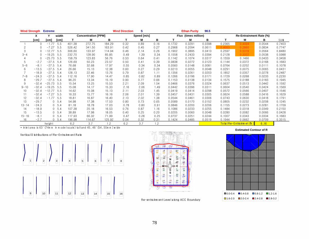
Wind Strength Wind Direction Ethan Purity

0.44940.4053 0.2860

0.5319

0.3322

Extreme S 98.5X Y width

[cm] [cm] [cm] T M B T M B T M B T M B SU M

1 0 -1.77 5.5 401.38 272.75 184.29 0.32 0.89 0.16 0.1732 0.3291 0.0398 0.2365 0.0544 0.74032 0 -7.27 5.5 526.42 341.50 163.91 0.42 0.45 0.27 0.2968 0.2094 0.0611 0.0834 0.7747

3 0 -12.77 5.5 306.60 133.97 114.94 0.46 2.14 0.26 0.1902 0.3895 0.0413 0.2597 0.0564 0.8480

3-4 0 -19.25 5.5 232.70 128.90 85.85 0.49 1.39 0.34 0.1558 0.2433 0.0394 0.2128 0.0538 0.5988

4 0 -25.73 5.5 158.79 123.83 56.76 0.53 0.64 0.41 0.1142 0.1074 0.0317 0.1559 0.1466 0.0433 0.3458

5 -2.7 -27.5 5.4 126.69 50.23 23.57 0.50 0.41 0.39 0.0838 0.0272 0.0123 0.1144 0.0372 0.0168 0.1683

5-6 -8.1 -27.5 5.4 76.68 32.68 17.97 0.55 0.34 0.34 0.0560 0.0148 0.0081 0.0764 0.0202 0.0111 0.1078

6 -13.5 -27.5 5.4 26.66 15.13 12.38 0.60 0.27 0.29 0.0213 0.0055 0.0048 0.0291 0.0075 0.0065 0.04317 -18.9 -27.5 5.4 128.13 22.46 13.76 0.79 0.87 1.11 0.1356 0.0261 0.0203 0.1852 0.0357 0.0278 0.2487

7-8 -24.3 -27.5 5.4 112.16 17.90 14.47 0.85 0.82 0.89 0.1266 0.0196 0.0171 0.1729 0.0268 0.0233 0.2230

8 -29.7 -27.5 5.4 96.20 13.34 15.19 0.90 0.77 0.66 0.1153 0.0138 0.0134 0.1575 0.0188 0.0183 0.1945

9 -32.4 -25.73 5.5 15.54 13.25 15.53 2.21 2.09 1.54 0.0466 0.0376 0.0324 0.0637 0.0513 0.0442 0.1592

9-10 -32.4 -19.25 5.5 15.08 14.17 15.33 2.16 2.06 1.49 0.0442 0.0396 0.0311 0.0604 0.0540 0.0424 0.1569

10 -32.4 -12.77 5.5 14.62 15.08 15.13 2.11 2.03 1.45 0.0419 0.0414 0.0298 0.0572 0.0566 0.0407 0.154611 -32.4 -7.27 5.5 16.33 15.77 16.16 2.06 2.01 1.39 0.0457 0.0431 0.0305 0.0624 0.0588 0.0416 0.1629

12 -32.4 -1.77 5.5 18.81 16.87 16.40 2.13 2.02 1.38 0.0544 0.0461 0.0306 0.0743 0.0630 0.0418 0.1791

13 -29.7 0 5.4 54.98 17.38 17.53 0.80 0.73 0.65 0.0589 0.0170 0.0152 0.0805 0.0232 0.0208 0.1245

13-14 -24.3 0 5.4 81.18 18.78 17.03 0.78 0.80 0.91 0.0846 0.0200 0.0206 0.1155 0.0273 0.0281 0.1709

14 -18.9 0 5.4 107.38 20.18 16.53 0.76 0.87 1.16 0.1086 0.0233 0.0255 0.1484 0.0318 0.0349 0.2150

15 -13.5 0 5.4 38.89 17.98 18.05 0.40 0.25 0.20 0.0205 0.0060 0.0048 0.0280 0.0082 0.0066 0.0428

15-16 -8.1 0 5.4 117.93 66.32 71.99 0.47 0.28 0.25 0.0737 0.0251 0.0244 0.1007 0.0343 0.0334 0.168316 -2.7 0 5.4 196.98 114.67 125.92 0.54 0.32 0.31 0.1424 0.0485 0.0519 0.1944 0.0662 0.0709 0.3315

height 6.2 3.7 1.2 6.2 3.7 1.2 6.16

* Inlet area is 63' (74m m in m odel scale) tall and 45, 46' (54, 55m m ) w ide

Vertical D istributions of R e-Entrainm ent R ate

R e-entrainm ent Level along A C C B oundary

Total R e-Entrainm et (% )

Re-Entrainment Rate (%)Concentration [PPM] Speed [m/s] Flux (times million)

1 2 3 4 5 6 7 8

9 10 11 12 13 14 15 16

N

E

S

W

Estimated Contour of R

0.0-0.4 0.4-0.8 0.8-1.2 1.2-1.6

1.6-2.0 2.0-2.4 2.4-2.8 2.8-3.2

78

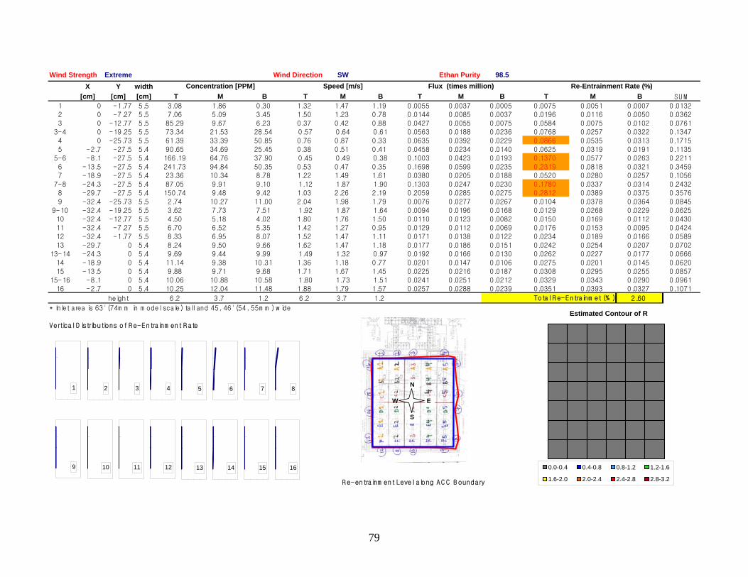
Wind Strength Wind Direction Ethan Purity

0.0866

0.1370

0.2319

0.1780

0.2812

0.0104

Extreme SW 98.5X Y width

[cm] [cm] [cm] T M B T M B T M B T M B SU M

1 0 -1.77 5.5 3.08 1.86 0.30 1.32 1.47 1.19 0.0055 0.0037 0.0005 0.0075 0.0051 0.0007 0.01322 0 -7.27 5.5 7.06 5.09 3.45 1.50 1.23 0.78 0.0144 0.0085 0.0037 0.0196 0.0116 0.0050 0.0362

3 0 -12.77 5.5 85.29 9.67 6.23 0.37 0.42 0.88 0.0427 0.0055 0.0075 0.0584 0.0075 0.0102 0.0761

3-4 0 -19.25 5.5 73.34 21.53 28.54 0.57 0.64 0.61 0.0563 0.0188 0.0236 0.0768 0.0257 0.0322 0.1347

4 0 -25.73 5.5 61.39 33.39 50.85 0.76 0.87 0.33 0.0635 0.0392 0.0229 0.0535 0.0313 0.1715

5 -2.7 -27.5 5.4 90.65 34.69 25.45 0.38 0.51 0.41 0.0458 0.0234 0.0140 0.0625 0.0319 0.0191 0.1135

5-6 -8.1 -27.5 5.4 166.19 64.76 37.90 0.45 0.49 0.38 0.1003 0.0423 0.0193 0.0577 0.0263 0.2211

6 -13.5 -27.5 5.4 241.73 94.84 50.35 0.53 0.47 0.35 0.1698 0.0599 0.0235 0.0818 0.0321 0.34597 -18.9 -27.5 5.4 23.36 10.34 8.78 1.22 1.49 1.61 0.0380 0.0205 0.0188 0.0520 0.0280 0.0257 0.1056

7-8 -24.3 -27.5 5.4 87.05 9.91 9.10 1.12 1.87 1.90 0.1303 0.0247 0.0230 0.0337 0.0314 0.2432

8 -29.7 -27.5 5.4 150.74 9.48 9.42 1.03 2.26 2.19 0.2059 0.0285 0.0275 0.0389 0.0375 0.3576

9 -32.4 -25.73 5.5 2.74 10.27 11.00 2.04 1.98 1.79 0.0076 0.0277 0.0267 0.0378 0.0364 0.0845

9-10 -32.4 -19.25 5.5 3.62 7.73 7.51 1.92 1.87 1.64 0.0094 0.0196 0.0168 0.0129 0.0268 0.0229 0.0625

10 -32.4 -12.77 5.5 4.50 5.18 4.02 1.80 1.76 1.50 0.0110 0.0123 0.0082 0.0150 0.0169 0.0112 0.043011 -32.4 -7.27 5.5 6.70 6.52 5.35 1.42 1.27 0.95 0.0129 0.0112 0.0069 0.0176 0.0153 0.0095 0.0424

12 -32.4 -1.77 5.5 8.33 6.95 8.07 1.52 1.47 1.11 0.0171 0.0138 0.0122 0.0234 0.0189 0.0166 0.0589

13 -29.7 0 5.4 8.24 9.50 9.66 1.62 1.47 1.18 0.0177 0.0186 0.0151 0.0242 0.0254 0.0207 0.0702

13-14 -24.3 0 5.4 9.69 9.44 9.99 1.49 1.32 0.97 0.0192 0.0166 0.0130 0.0262 0.0227 0.0177 0.0666

14 -18.9 0 5.4 11.14 9.38 10.31 1.36 1.18 0.77 0.0201 0.0147 0.0106 0.0275 0.0201 0.0145 0.0620

15 -13.5 0 5.4 9.88 9.71 9.68 1.71 1.67 1.45 0.0225 0.0216 0.0187 0.0308 0.0295 0.0255 0.0857

15-16 -8.1 0 5.4 10.06 10.88 10.58 1.80 1.73 1.51 0.0241 0.0251 0.0212 0.0329 0.0343 0.0290 0.096116 -2.7 0 5.4 10.25 12.04 11.48 1.88 1.79 1.57 0.0257 0.0288 0.0239 0.0351 0.0393 0.0327 0.1071

height 6.2 3.7 1.2 6.2 3.7 1.2 2.60

* Inlet area is 63' (74m m in m odel scale) tall and 45, 46' (54, 55m m ) w ide

Vertical D istributions of R e-Entrainm ent R ate

R e-entrainm ent Level along A C C B oundary

Total R e-Entrainm et (% )

Re-Entrainment Rate (%)Concentration [PPM] Speed [m/s] Flux (times million)

1 2 3 4 5 6 7 8

9 10 11 12 13 14 15 16

N

E

S

W

Estimated Contour of R

0.0-0.4 0.4-0.8 0.8-1.2 1.2-1.6

1.6-2.0 2.0-2.4 2.4-2.8 2.8-3.2

79

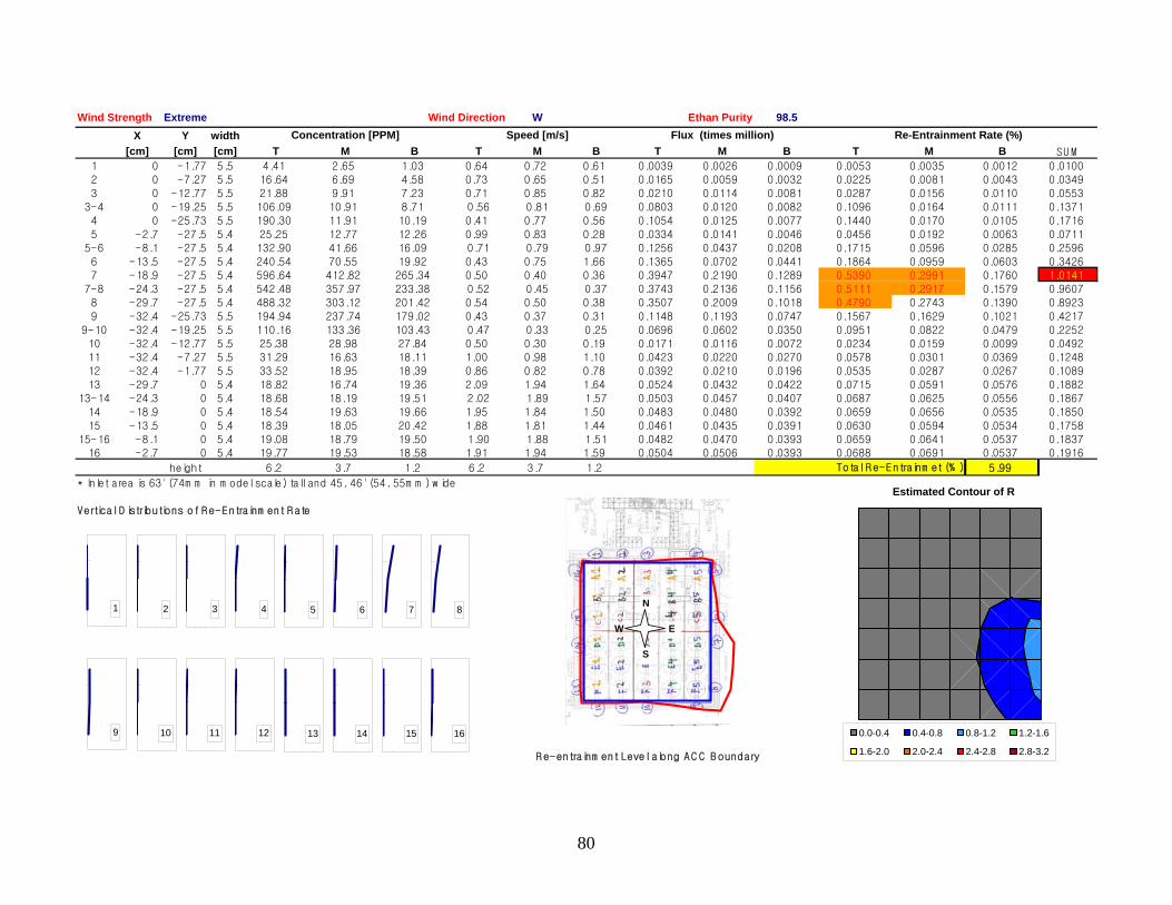
Wind Strength Wind Direction Ethan Purity

0.5390 0.2991

0.5111 0.2917

0.4790

0.1567

Extreme W 98.5X Y width

[cm] [cm] [cm] T M B T M B T M B T M B SU M

1 0 -1.77 5.5 4.41 2.65 1.03 0.64 0.72 0.61 0.0039 0.0026 0.0009 0.0053 0.0035 0.0012 0.01002 0 -7.27 5.5 16.64 6.69 4.58 0.73 0.65 0.51 0.0165 0.0059 0.0032 0.0225 0.0081 0.0043 0.0349

3 0 -12.77 5.5 21.88 9.91 7.23 0.71 0.85 0.82 0.0210 0.0114 0.0081 0.0287 0.0156 0.0110 0.0553

3-4 0 -19.25 5.5 106.09 10.91 8.71 0.56 0.81 0.69 0.0803 0.0120 0.0082 0.1096 0.0164 0.0111 0.1371

4 0 -25.73 5.5 190.30 11.91 10.19 0.41 0.77 0.56 0.1054 0.0125 0.0077 0.1440 0.0170 0.0105 0.1716

5 -2.7 -27.5 5.4 25.25 12.77 12.26 0.99 0.83 0.28 0.0334 0.0141 0.0046 0.0456 0.0192 0.0063 0.0711

5-6 -8.1 -27.5 5.4 132.90 41.66 16.09 0.71 0.79 0.97 0.1256 0.0437 0.0208 0.1715 0.0596 0.0285 0.2596

6 -13.5 -27.5 5.4 240.54 70.55 19.92 0.43 0.75 1.66 0.1365 0.0702 0.0441 0.1864 0.0959 0.0603 0.34267 -18.9 -27.5 5.4 596.64 412.82 265.34 0.50 0.40 0.36 0.3947 0.2190 0.1289 0.1760 1.0141

7-8 -24.3 -27.5 5.4 542.48 357.97 233.38 0.52 0.45 0.37 0.3743 0.2136 0.1156 0.1579 0.9607

8 -29.7 -27.5 5.4 488.32 303.12 201.42 0.54 0.50 0.38 0.3507 0.2009 0.1018 0.2743 0.1390 0.8923

9 -32.4 -25.73 5.5 194.94 237.74 179.02 0.43 0.37 0.31 0.1148 0.1193 0.0747 0.1629 0.1021 0.4217

9-10 -32.4 -19.25 5.5 110.16 133.36 103.43 0.47 0.33 0.25 0.0696 0.0602 0.0350 0.0951 0.0822 0.0479 0.2252

10 -32.4 -12.77 5.5 25.38 28.98 27.84 0.50 0.30 0.19 0.0171 0.0116 0.0072 0.0234 0.0159 0.0099 0.049211 -32.4 -7.27 5.5 31.29 16.63 18.11 1.00 0.98 1.10 0.0423 0.0220 0.0270 0.0578 0.0301 0.0369 0.1248

12 -32.4 -1.77 5.5 33.52 18.95 18.39 0.86 0.82 0.78 0.0392 0.0210 0.0196 0.0535 0.0287 0.0267 0.1089

13 -29.7 0 5.4 18.82 16.74 19.36 2.09 1.94 1.64 0.0524 0.0432 0.0422 0.0715 0.0591 0.0576 0.1882

13-14 -24.3 0 5.4 18.68 18.19 19.51 2.02 1.89 1.57 0.0503 0.0457 0.0407 0.0687 0.0625 0.0556 0.1867

14 -18.9 0 5.4 18.54 19.63 19.66 1.95 1.84 1.50 0.0483 0.0480 0.0392 0.0659 0.0656 0.0535 0.1850

15 -13.5 0 5.4 18.39 18.05 20.42 1.88 1.81 1.44 0.0461 0.0435 0.0391 0.0630 0.0594 0.0534 0.1758

15-16 -8.1 0 5.4 19.08 18.79 19.50 1.90 1.88 1.51 0.0482 0.0470 0.0393 0.0659 0.0641 0.0537 0.183716 -2.7 0 5.4 19.77 19.53 18.58 1.91 1.94 1.59 0.0504 0.0506 0.0393 0.0688 0.0691 0.0537 0.1916

height 6.2 3.7 1.2 6.2 3.7 1.2 5.99

* Inlet area is 63' (74m m in m odel scale) tall and 45, 46' (54, 55m m ) w ide

Vertical D istributions of R e-Entrainm ent R ate

R e-entrainm ent Level along A C C B oundary

Total R e-Entrainm et (% )

Re-Entrainment Rate (%)Concentration [PPM] Speed [m/s] Flux (times million)

1 2 3 4 5 6 7 8

9 10 11 12 13 14 15 16

N

E

S

W

Estimated Contour of R

0.0-0.4 0.4-0.8 0.8-1.2 1.2-1.6

1.6-2.0 2.0-2.4 2.4-2.8 2.8-3.2

80

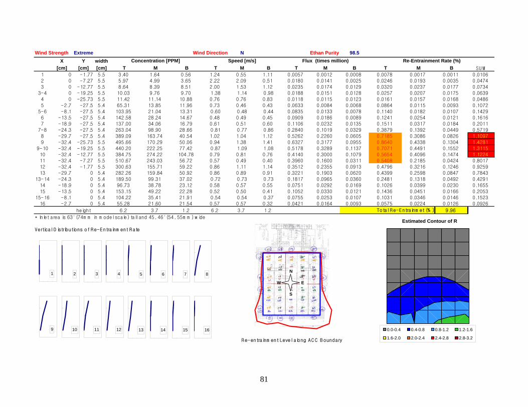
Wind Strength Wind Direction Ethan Purity

0.7185

0.8640

0.7071

0.56540.5408

Extreme N 98.5X Y width

[cm] [cm] [cm] T M B T M B T M B T M B SU M

1 0 -1.77 5.5 3.40 1.64 0.56 1.24 0.55 1.11 0.0057 0.0012 0.0008 0.0078 0.0017 0.0011 0.01062 0 -7.27 5.5 5.97 4.99 3.65 2.22 2.09 0.51 0.0180 0.0141 0.0025 0.0246 0.0193 0.0035 0.0474

3 0 -12.77 5.5 8.64 8.39 8.51 2.00 1.53 1.12 0.0235 0.0174 0.0129 0.0320 0.0237 0.0177 0.0734

3-4 0 -19.25 5.5 10.03 9.76 9.70 1.38 1.14 0.98 0.0188 0.0151 0.0128 0.0257 0.0207 0.0175 0.0639

4 0 -25.73 5.5 11.42 11.14 10.88 0.76 0.76 0.83 0.0118 0.0115 0.0123 0.0161 0.0157 0.0168 0.0486

5 -2.7 -27.5 5.4 65.31 13.85 11.96 0.73 0.46 0.43 0.0633 0.0084 0.0068 0.0864 0.0115 0.0093 0.1072

5-6 -8.1 -27.5 5.4 103.95 21.04 13.31 0.60 0.48 0.44 0.0835 0.0133 0.0078 0.1140 0.0182 0.0107 0.1429

6 -13.5 -27.5 5.4 142.58 28.24 14.67 0.48 0.49 0.45 0.0909 0.0186 0.0089 0.1241 0.0254 0.0121 0.16167 -18.9 -27.5 5.4 137.00 34.06 16.79 0.61 0.51 0.60 0.1106 0.0232 0.0135 0.1511 0.0317 0.0184 0.2011

7-8 -24.3 -27.5 5.4 263.04 98.90 28.66 0.81 0.77 0.86 0.2840 0.1019 0.0329 0.3879 0.1392 0.0449 0.5719

8 -29.7 -27.5 5.4 389.09 163.74 40.54 1.02 1.04 1.12 0.5262 0.2260 0.0605 0.3086 0.0826 1.1097

9 -32.4 -25.73 5.5 495.66 170.29 50.06 0.94 1.38 1.41 0.6327 0.3177 0.0955 0.4338 0.1304 1.4281

9-10 -32.4 -19.25 5.5 440.20 222.25 77.42 0.87 1.09 1.08 0.5178 0.3289 0.1137 0.4491 0.1552 1.3115

10 -32.4 -12.77 5.5 384.75 274.22 104.78 0.79 0.81 0.76 0.4140 0.3000 0.1079 0.4096 0.1474 1.122411 -32.4 -7.27 5.5 510.67 243.03 56.72 0.57 0.49 0.40 0.3960 0.1600 0.0311 0.2185 0.0424 0.8017

12 -32.4 -1.77 5.5 300.63 155.71 59.22 0.86 1.11 1.14 0.3512 0.2355 0.0913 0.4796 0.3216 0.1246 0.9259

13 -29.7 0 5.4 282.26 159.84 50.92 0.86 0.89 0.91 0.3221 0.1903 0.0620 0.4399 0.2598 0.0847 0.7843

13-14 -24.3 0 5.4 189.50 99.31 37.02 0.72 0.73 0.73 0.1817 0.0965 0.0360 0.2481 0.1318 0.0492 0.4291

14 -18.9 0 5.4 96.73 38.78 23.12 0.58 0.57 0.55 0.0751 0.0292 0.0169 0.1026 0.0399 0.0230 0.1655

15 -13.5 0 5.4 153.15 49.22 22.28 0.52 0.50 0.41 0.1052 0.0330 0.0121 0.1436 0.0451 0.0166 0.2053

15-16 -8.1 0 5.4 104.22 35.41 21.91 0.54 0.54 0.37 0.0755 0.0253 0.0107 0.1031 0.0346 0.0146 0.152316 -2.7 0 5.4 55.28 21.60 21.54 0.57 0.57 0.32 0.0421 0.0164 0.0093 0.0575 0.0224 0.0126 0.0926

height 6.2 3.7 1.2 6.2 3.7 1.2 9.96

* Inlet area is 63' (74m m in m odel scale) tall and 45, 46' (54, 55m m ) w ide

Vertical D istributions of R e-Entrainm ent R ate

R e-entrainm ent Level along A C C B oundary

Total R e-Entrainm et (% )

Re-Entrainment Rate (%)Concentration [PPM] Speed [m/s] Flux (times million)

1 2 3 4 5 6 7 8

9 10 11 12 13 14 15 16

N

E

S

W

Estimated Contour of R

0.0-0.4 0.4-0.8 0.8-1.2 1.2-1.6

1.6-2.0 2.0-2.4 2.4-2.8 2.8-3.2

81

82

Appendix – B Testing Results of the Dual Unit Base Model

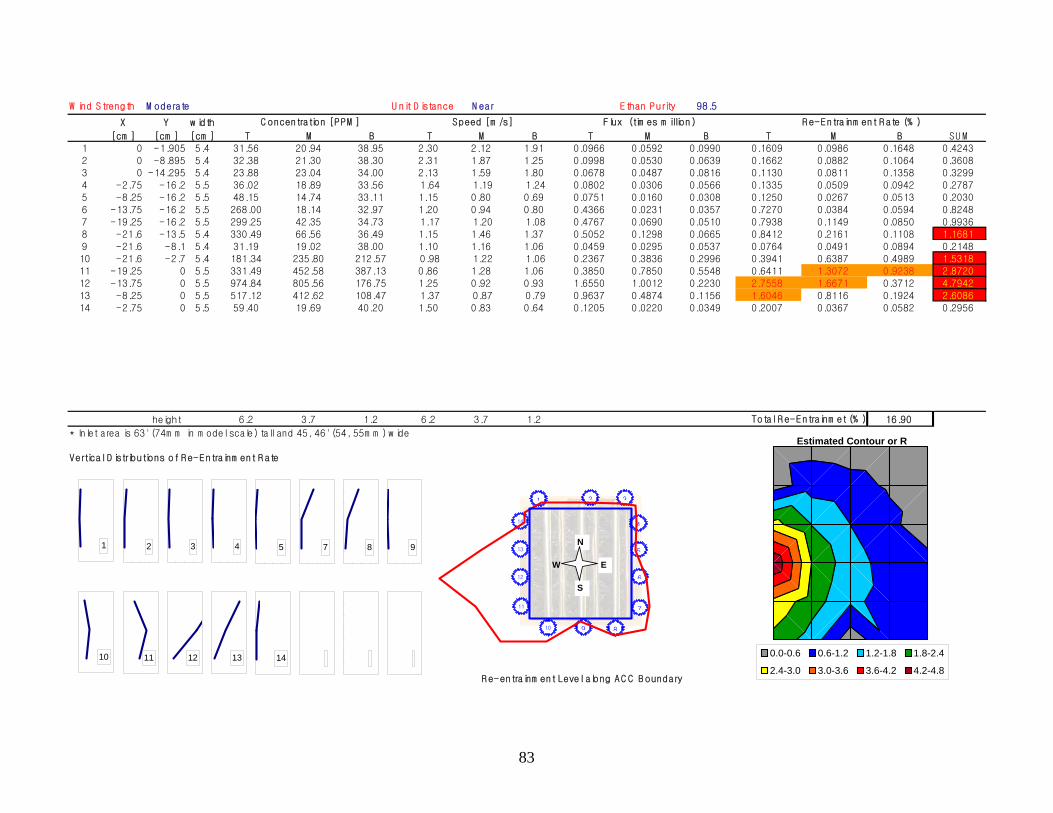
W ind Strength U nit D istance Ethan Purity

1.3072 0.9238

2.7558 1.6671

1.6046

M oderate N ear 98.5

X Y w idth

[cm ] [cm ] [cm ] T M B T M B T M B T M B SU M

1 0 -1.905 5.4 31.56 20.94 38.95 2.30 2.12 1.91 0.0966 0.0592 0.0990 0.1609 0.0986 0.1648 0.4243

2 0 -8.895 5.4 32.38 21.30 38.30 2.31 1.87 1.25 0.0998 0.0530 0.0639 0.1662 0.0882 0.1064 0.36083 0 -14.295 5.4 23.88 23.04 34.00 2.13 1.59 1.80 0.0678 0.0487 0.0816 0.1130 0.0811 0.1358 0.3299

4 -2.75 -16.2 5.5 36.02 18.89 33.56 1.64 1.19 1.24 0.0802 0.0306 0.0566 0.1335 0.0509 0.0942 0.2787

5 -8.25 -16.2 5.5 48.15 14.74 33.11 1.15 0.80 0.69 0.0751 0.0160 0.0308 0.1250 0.0267 0.0513 0.2030

6 -13.75 -16.2 5.5 268.00 18.14 32.97 1.20 0.94 0.80 0.4366 0.0231 0.0357 0.7270 0.0384 0.0594 0.8248

7 -19.25 -16.2 5.5 299.25 42.35 34.73 1.17 1.20 1.08 0.4767 0.0690 0.0510 0.7938 0.1149 0.0850 0.9936

8 -21.6 -13.5 5.4 330.49 66.56 36.49 1.15 1.46 1.37 0.5052 0.1298 0.0665 0.8412 0.2161 0.1108 1.1681

9 -21.6 -8.1 5.4 31.19 19.02 38.00 1.10 1.16 1.06 0.0459 0.0295 0.0537 0.0764 0.0491 0.0894 0.214810 -21.6 -2.7 5.4 181.34 235.80 212.57 0.98 1.22 1.06 0.2367 0.3836 0.2996 0.3941 0.6387 0.4989 1.5318

11 -19.25 0 5.5 331.49 452.58 387.13 0.86 1.28 1.06 0.3850 0.7850 0.5548 0.6411 2.8720

12 -13.75 0 5.5 974.84 805.56 176.75 1.25 0.92 0.93 1.6550 1.0012 0.2230 0.3712 4.7942

13 -8.25 0 5.5 517.12 412.62 108.47 1.37 0.87 0.79 0.9637 0.4874 0.1156 0.8116 0.1924 2.6086

14 -2.75 0 5.5 59.40 19.69 40.20 1.50 0.83 0.64 0.1205 0.0220 0.0349 0.2007 0.0367 0.0582 0.2956

height 6.2 3.7 1.2 6.2 3.7 1.2 16.90

* Inlet area is 63' (74m m in m odel scale) tall and 45, 46' (54, 55m m ) w ide

Vertical D istributions of R e-Entrainm ent R ate

R e-entrainm ent Level along A C C B oundary

Total R e-Entrainm et (% )

R e-Entrainm ent R ate (% )C oncentration [PPM ] Speed [m /s] Flux (tim es m illion)

1 2 3

4

5

6

7

8910

11

12

13

14

1 2 3 4 5 7 8 9

10 11 12 13 14

N

E

S

W

Estimated Contour or R

0.0-0.6 0.6-1.2 1.2-1.8 1.8-2.4

2.4-3.0 3.0-3.6 3.6-4.2 4.2-4.8

83

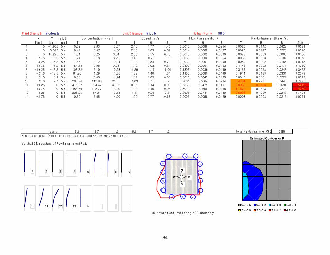
W ind Strength U nit D istance Ethan Purity

0.4764

0.8939 0.5786

1.1672

0.6004

M oderate M iddle 98.5

X Y w idth

[cm ] [cm ] [cm ] T M B T M B T M B T M B SU M

1 0 -1.905 5.4 0.52 3.63 13.07 2.16 1.77 1.46 0.0015 0.0086 0.0254 0.0025 0.0142 0.0423 0.0591

2 0 -8.895 5.4 0.47 6.07 14.88 2.18 1.09 0.69 0.0014 0.0088 0.0137 0.0023 0.0147 0.0228 0.03983 0 -14.295 5.4 1.61 0.25 6.31 2.03 0.55 0.43 0.0043 0.0002 0.0036 0.0072 0.0003 0.0060 0.0136

4 -2.75 -16.2 5.5 1.74 0.18 8.28 1.61 0.70 0.57 0.0038 0.0002 0.0064 0.0063 0.0003 0.0107 0.0173

5 -8.25 -16.2 5.5 1.86 0.12 10.24 1.19 0.84 0.71 0.0030 0.0001 0.0099 0.0050 0.0002 0.0165 0.0218

6 -13.75 -16.2 5.5 154.68 0.08 9.31 1.19 0.93 0.81 0.2490 0.0001 0.0103 0.4146 0.0002 0.0171 0.4319

7 -19.25 -16.2 5.5 108.32 2.19 10.33 1.29 1.17 1.06 0.1896 0.0035 0.0149 0.3156 0.0058 0.0248 0.3462

8 -21.6 -13.5 5.4 61.96 4.29 11.35 1.39 1.40 1.31 0.1150 0.0080 0.0199 0.1914 0.0133 0.0331 0.2379

9 -21.6 -8.1 5.4 0.66 3.48 11.74 1.11 1.05 0.85 0.0010 0.0049 0.0133 0.0016 0.0081 0.0222 0.031910 -21.6 -2.7 5.4 208.24 113.98 21.85 1.03 1.10 0.91 0.2861 0.1664 0.0264 0.2771 0.0440 0.7975

11 -19.25 0 5.5 415.82 224.47 31.95 0.95 1.14 0.96 0.5368 0.3475 0.0417 0.0694 1.5419

12 -13.75 0 5.5 453.60 108.77 13.09 1.14 1.15 0.94 0.7010 0.1699 0.0168 0.2828 0.0279 1.4779

13 -8.25 0 5.5 226.95 57.21 13.54 1.17 0.96 0.81 0.3606 0.0744 0.0149 0.1239 0.0248 0.7491

14 -2.75 0 5.5 0.30 5.65 14.00 1.20 0.77 0.68 0.0005 0.0059 0.0129 0.0008 0.0098 0.0215 0.0321

height 6.2 3.7 1.2 6.2 3.7 1.2 5.80

* Inlet area is 63' (74m m in m odel scale) tall and 45, 46' (54, 55m m ) w ide

Vertical D istributions of R e-Entrainm ent R ate

R e-entrainm ent Level along A C C B oundary

Total R e-Entrainm et (% )

R e-Entrainm ent R ate (% )C oncentration [PPM ] Speed [m /s] Flux (tim es m illion)

1 2 3

4

5

6

7

8910

11

12

13

14

1 2 3 4 5 7 8 9

10 11 12 13 14

N

E

S

W

Estimated Contour or R

0.0-0.6 0.6-1.2 1.2-1.8 1.8-2.4

2.4-3.0 3.0-3.6 3.6-4.2 4.2-4.8

84

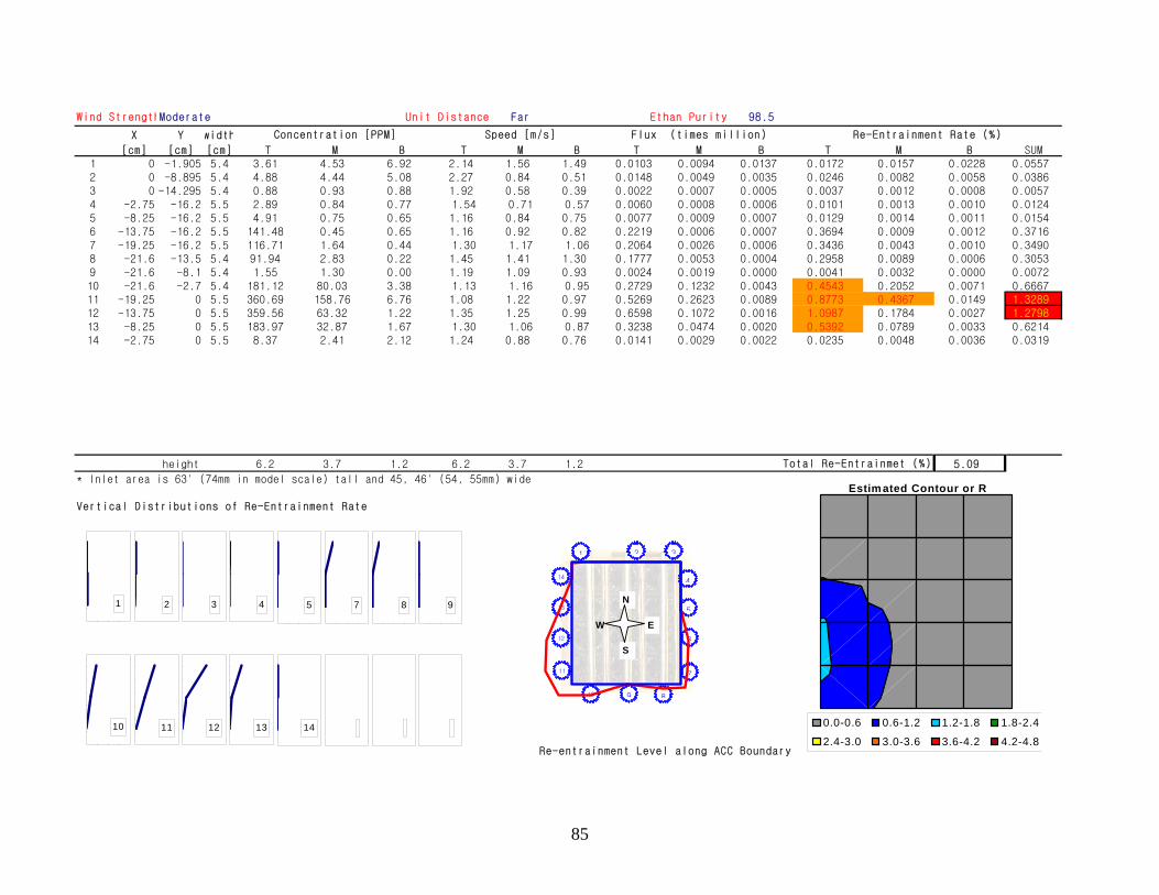
Wind StrengthModerate Far 98.5

X Y

Unit Distance Ethan Purity

width

[cm] [cm] [cm] T M B T M B T M B T M B SUM1 0 -1.905 5.4 3.61 4.53 6.92 2.14 1.56 1.49 0.0103 0.0094 0.0137 0.0172 0.0157 0.0228 0.05572 0 -8.895 5.4 4.88 4.44 5.08 2.27 0.84 0.51 0.0148 0.0049 0.0035 0.0246 0.0082 0.0058 0.03863 0 -14.295 5.4 0.88 0.93 0.88 1.92 0.58 0.39 0.0022 0.0007 0.0005 0.0037 0.0012 0.0008 0.00574 -2.75 -16.2 5.5 2.89 0.84 0.77 1.54 0.71 0.57 0.0060 0.0008 0.0006 0.0101 0.0013 0.0010 0.01245 -8.25 -16.2 5.5 4.91 0.75 0.65 1.16 0.84 0.75 0.0077 0.0009 0.0007 0.0129 0.0014 0.0011 0.01546 -13.75 -16.2 5.5 141.48 0.45 0.65 1.16 0.92 0.82 0.2219 0.0006 0.0007 0.3694 0.0009 0.0012 0.37167 -19.25 -16.2 5.5 116.71 1.64 0.44 1.30 1.17 1.06 0.2064 0.0026 0.0006 0.3436 0.0043 0.0010 0.34908 -21.6 -13.5 5.4 91.94 2.83 0.22 1.45 1.41 1.30 0.1777 0.0053 0.0004 0.2958 0.0089 0.0006 0.30539 -21.6 -8.1 5.4 1.55 1.30 0.00 1.19 1.09 0.93 0.0024 0.0019 0.0000 0.0041 0.0032 0.0000 0.007210 -21.6 -2.7 5.4 181.12 80.03 3.38 1.13 1.16 0.95 0.2729 0.1232 0.0043 0.2052 0.0071 0.666711 -19.25 0 5.5 360.69 158.76 6.76 1.08 1.22 0.97 0.5269 0.2623 0.0089 0.0149 1.328912 -13.75 0 5.5 359.56 63.32 1.22 1.35 1.25 0.99 0.6598 0.1072 0.0016 0.0027 1.279813 -8.25 0 5.5 183.97 32.87 1.67 1.30 1.06 0.87 0.3238 0.0474 0.0020 0.0789 0.0033 0.621414 -2.75 0 5.5 8.37 2.41 2.12 1.24 0.88 0.76 0.0141 0.0029 0.0022 0.0235 0.0048 0.0036 0.0319

height 6.2 3.7 1.2 6.2 3.7 1.2 5.09

* Inlet area is 63' (74mm in model scale) tall and 45, 46' (54, 55mm) wide

Vertical Distributions of Re-Entrainment Rate

Re-entrainment Level along ACC Boundary

Total Re-Entrainmet (%)

Re-Entrainment Rate (%)Concentration [PPM] Speed [m/s] Flux (times million)

0.45430.8773 0.43671.0987 0.17840.5392

1 2 3

4

5

6

7

8910

11

12

13

14

1 2 3 4 5 7 8 9

10 11 12 13 14

N

E

S

W

Estim ated Contour or R

0.0-0.6 0.6-1.2 1.2-1.8 1.8-2.4

2.4-3.0 3.0-3.6 3.6-4.2 4.2-4.8

85