1

Supplementary material of the article submitted to Precision Agriculture

A Wireless Sensor Network-based Monitoring System with Dynamic

Convergecast Tree Algorithm for Precision Cultivation Management in

Orchid Greenhouses

Authors:

Joe-Air Jianga,b,c,*, Chien-Hao Wanga,�, Min-Sheng Liaoa,�, Xiang-Yao Zhenga, Jen-Hao Liua,

Cheng-Long Chuangc,d, Che-Lun Hunge, and Chia-Pang Chenf,†

Affiliations of Authors: a Department of Bio-Industrial Mechatronics Engineering, National Taiwan University, Taipei

10617, Taiwan. b Education and Research Center for Bio-Industrial Automation, National Taiwan University, Taipei

10617, Taiwan. c Intel-NTU Connected Context Computing Center, National Taiwan University, Taipei 10617,

Taiwan. d Intel Labs, Intel Corporation, Hillsboro, OR 97124, USA. e Department of Computer Science and Communication Engineering, Providence University,

No.200, Sec. 7, Taiwan Blvd., Taichung 433, Taiwan. f MOXA Inc., New Taipei City 23145, Taiwan. # Equal Contribution

*Corresponding Author:

Joe-Air Jiang, Professor, Ph.D., P.Eng.

Department of Bio-Industrial Mechatronics Engineering

National Taiwan University

No. 1, Roosevelt Rd., Sec. 4, Taipei 10617, Taiwan

Phone: + 886-2-3366-5341, Fax: +886-2-2362-7620

E-mail: jajiang@ntu.edu.tw

2

* This document is a supplementary material accompanying with the paper entitled “A Wireless Sensor

Network-based Monitoring System with Dynamic Convergecast Tree Algorithm for Precision

Cultivation Management in Modern Orchid Greenhouses”. It provides experimental test results for

readers to have a better understanding of the basic performance of the proposed algorithm using a single

mobile node, two mobile nodes, and multiple mobile nodes in a classroom environment. The performance of

overhead and power consumption with different algorithms is compared. In addition, the procedures of the

semi-variogram analysis and the kriging method used in the proposed article are also introduced in the

supplementary material. Please feel no hesitate to contact the corresponding author if further assistances

are required.

Corresponding Author: Prof. Joe-Air Jiang, Ph.D.

E-mail address: jajiang@ntu.edu.tw

3

Basic performance evaluation of the proposed algorithm using a single mobile node, two mobile nodes, and multiple mobile nodes

in a classroom environment

S.0 Introduction

This study aims to design a special routing algorithm that can adapt to dynamic WSNs with changeable topologies

to provide reliable monitoring data. To evaluate the performance of the proposed algorithm in terms of successful rates

of data delivery, a number of possible moving paths were designed in a classroom environment to simulate the

movement scenarios of movable benches in a greenhouse. The main purpose of the feasibility test done in the classroom

was to examine whether the proposed DTCA could deal with multiple targets and varying paths in different scenarios.

Although the classroom was smaller than a real greenhouse, dense packet collision caused by the multipath effect may

still occur. In the following subsections, each experiment is described in detail.

S.1 Experiments conducted in a classroom environment

The experimental site was a classroom at the campus of National Taiwan University. The dimension of the

experimental room was 11 m × 6.9 m × 2.8 m. Twenty nodes were deployed. Among these nodes, 15 nodes (no. 2 to

no. 16) were placed on the wall and served as the anchor nodes. Some nodes moved manually served as the mobile

nodes moving along the preset routes to test the performance of the proposed algorithm. A gateway was hung on the

right-side wall. It collected the sensed data and communicated with all sensor nodes. The physical deployment is shown

in Figure 10. In the experiments, the fixed and mobile nodes formed a dynamic tree topology every 15 s. It meant that

all of the sensed data coming from the nodes in the WSN would be collected by the gateway every 15 s. Note that the

packet size of all sensor data was 26 bytes, the same size as the packets transmitted in the automatically controlled

orchid greenhouse which will be discussed in the following sub-section. The packet included the basic information of

the sensor node, such as the header, the cyclic redundancy check (CRC) code and the sensed data of environmental

parameters, such as temperature, humidity and illumination. The purpose of the intensive network update was to verify

the robustness of the proposed DCTA.

Figure S. 1 The physical deployment of a WSN tested in a classroom at the NTU campus

4

S.2 Data delivery rate of the deployed network

In this study, the successful rates of data delivery in each testing round for the entire network, fixed nodes, and

mobile nodes in the deployed WSN were respectively defined as

( )100%,EnrireNetwork

Packets from Fix Mobile Nodes Recieved by GatewaySuccRate

Packets Sent by Fix Node Packets Sent by Mobile Node+

= ×+

∑∑ ∑ (1)

100%,FixNode

Packets from Fix Node Recieved by GatewaySuccRate

Packets Sent by Fix Node= ×∑

∑ (2) and

100%MobileNode

Packets from Mobile Node Recieved by GatewaySuccRate

Packets Sent by Mobile Node= ×∑

∑ (3) Note that SuccRateFixNode and SuccRateMobileNode represent the successful data delivery rates between the gateway and the

fixed nodes and mobile nodes in each testing round, respectively.

The average successful rates of data delivery of the total experimental rounds for the entire network, fixed nodes,

and mobile nodes in the deployed WSN were also respectively defined as

,EnrireNetworkEnrireNetwork

totoal

SuccRateAvgSuccRate

Round=∑

(4)

,FixNodeFixNode

total

SuccRateAvgSuccRate

Round=∑

(5) and

MobileNodeMobileNode

total

SuccRateAvgSuccRate

Round=∑

(6) Note that Roundtotal is the total rounds of the whole experiments.

S.3 Test case 1: Single Mobile Node

In this test case, one mobile node (no. 21) and four randomly deployed anchor nodes (no. 17~no. 20) were

selected and initially placed at a corner of the experimental room, as shown in Figure S.2a. This scenario was used to

simulate the case of a newly joined bench moving to a specific area or a bench moving to the spraying area from the

illuminating area. First, the gateway sent a command to initiate network operation without including the mobile node.

After the network was established, the mobile node was manually turned on, and then the network automatically

allowed the node to join it, following the dynamic update of the network topology and the time slot allocation in the

proposed DCTA. After that, the mobile node moved along the dotted line as shown in Figure S.2a with a speed of

around 0.22 m/sec. This speed was similar to the speed of the moving benches in a greenhouse. Ten measurements were

taken and the successful data delivery rate was computed, as shown in Figure S.2b. Successful data delivery meant that

a sensor node was able to successfully transmit the sensed data to the gateway. The results showed that the average

successful delivery rate for the mobile node and the entire network was 99.0% and 97.7%, respectively. Furthermore,

the test of successful data delivery was repeated ten times when the mobile node moved along a different route, as

shown in the dotted line in Figure S.3a, with a speed of around 0.18 m/sec. The movement path of the mobile node, e.g.

the node 21 in Figure S.3a, was along an “S”-shape path, which was pre-plotted on the ground in the classroom for

reference during experiments. Once the mobile node was carried by a person to pass an anchor node (say, node 20 in

Figure S.3a) and reach a turn point indicated on the ground, the movement would be changed by 90 degrees in a

5

counterclockwise direction. Such a movement continued to form an “S”-shape path, as shown in Figure S.3a. In this

experiment, each successful data delivery rate for the entire network in each measurement was higher than 95.0%, and

the average successful data delivery rate was 97.2%. The average successful data delivery rate for the mobile node was

98.7%. These results are shown in Figure S.3b, and they suggest that the proposed algorithm works well in a mobile

network. These two tests also indicate that the impact of the curved route and the moving speed for the mobile nodes on

the average successful data delivery rate is pretty small.

Figure S. 2 Test Case 1: only one single mobile node being deployed and moved along a rectangle route; (a) Layout of

the sensor network, (b) Successful data delivery rates

Figure S. 3 Test Case 1: only one single mobile node being deployed and moved along a more complicated route; (a)

Layout of the sensor network, (b) successful data delivery rates.

S.4 Test Case 2: Double Mobile Nodes

In this experiment, two mobile nodes (no. 20 and 21) were selected and started moving from the down right corner of

the experiment site, and three anchor nodes (no. 17~no.19) were placed randomly, as shown in Figure S.4a. Similar to

the case in the previous experiment, the gateway sent a command to ask all nodes but not the two mobile nodes to

establish a network. After the network was established, the two mobile nodes were turned on and started moving along

the dotted line with a speed of around 0.22 m/sec. The experimental results indicated that the average successful data

delivery rate for the two mobile nodes (no. 20 and node no. 21) was 98.6% and 96.5%, respectively. The average

successful data delivery rate for the entire network was 96.5%, as shown in Figure S.4b.

6

Moreover, an additional scenario was tested. In this scenario, the two nodes both moved along the route shown as

the dotted line in Figure S.5a with a speed of around 0.17 m/sec, and the test of the successful data delivery was

conducted ten times. Note that the “S”-shape path in this test was formed in the way similar to that of Figure S.3a. The

test results showed that the average successful data delivery rate for the two mobile nodes was 97.6% and 96.6%,

respectively. In addition, the average successful data delivery rate for the entire network was 96.7%. These results are

shown in Figure S.5b. An inspection of the results of these two tests indicates that differences in both the average

successful data delivery rates of the entire network and the mobile nodes are very small. This fact demonstrates that the

proposed DCTA is robust as the network topology changes.

Figure S. 4 Test Case 2: Double mobile nodes being deployed and moving along a rectangle route; (a) Layout of the

sensor network, (b)Successful data delivery rates

Figure S. 5 Test Case 2: Double mobile nodes being deployed and moving along a more complicated route; (a) Layout

of the sensor network, (b) Successful data delivery rates

S.5 Test Case 3: Multiple Mobile Nodes

To examine the adaptability of the algorithm under a more complicated dynamic environment, an experiment that

employed four mobile nodes (no. 17, 18, 20 and 21) was conducted. This experiment was used to determine whether the

proposed algorithm could adapt to a mobile network with multiple moving nodes. Especially, the two routes that the

mobile nodes moved along were allowed to intersect, as shown in Figure S.6a. The purpose of designing such moving

paths was to simulate the moving tracks of multiple benches and the situation in which the benches moved very close to

each other. The four nodes moved in the experimental site with a speed of around 0.11 m/s, and the test of the data

7

delivery was repeated ten times. The results of this experiment are shown in Figure S.6b. The average successful data

delivery rate for the four mobile nodes was 98.5%, 98.0%, 98.5% and 94.5%. Additionally, the average successful data

delivery rate for the entire network was still high at up to 97.8%. The results showed that the proposed algorithm, when

being applied to a complicated network with multiple mobile nodes, was able to successfully transmit the sensed data to

the gateway.

Figure S. 6 Test Case 3: The sensor network with multiple mobile nodes moving along an ‘S’-shaped route: (a) Layout

of the sensor network, (b) successful data delivery rates

S.6 Summary of the successful data delivery ratesAll of the results of the data delivery tests are summarized in Table 1. The results showed that the proposed DCTA

could maintain higher data delivery rates not only in the scenario of using a single mobile node but also in the scenario

of employing multiple mobile nodes, even when some complicated paths were involved. These results indicate that the

reliability can be guaranteed by using the proposed DCTA, because the DCTA benefits from an RSSI-based routing

strategy and flexible time slot allocation. By applying the DCTA to a WSN, better routing paths and well-arranged time

slots can avoid packet collision anytime, anywhere. Thus, the data transmission failure in the entire network can be

reduced significantly.

Table 1. Summary of the test results for the data delivery experiments conducted in a classroom

Single mobile Node Double mobile Nodes Multiple mobile nodes

simple path complicated path simple path complicated path

* of entire

network 97.7% 97% 96.48% 96.74% 97.82%

* of mobile nodes 99% 98.7% 98.56%,

96.48%

97.64%,

96.62%

98.5%, 98%,

98.5%, 95% * the average successful transmission rate

8

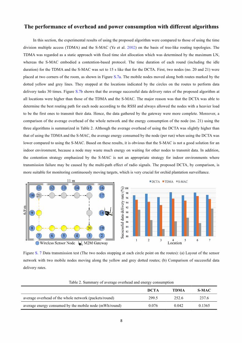
The performance of overhead and power consumption with different algorithms

In this section, the experimental results of using the proposed algorithm were compared to those of using the time

division multiple access (TDMA) and the S-MAC (Ye et al. 2002) on the basis of tree-like routing topologies. The

TDMA was regarded as a static approach with fixed time slot allocation which was determined by the maximum LN,

whereas the S-MAC embodied a contention-based protocol. The time duration of each round (including the idle

duration) for the TDMA and the S-MAC was set to 15 s like that for the DCTA. First, two nodes (no. 20 and 21) were

placed at two corners of the room, as shown in Figure S.7a. The mobile nodes moved along both routes marked by the

dotted yellow and grey lines. They stopped at the locations indicated by the circles on the routes to perform data

delivery tasks 30 times. Figure S.7b shows that the average successful data delivery rates of the proposed algorithm at

all locations were higher than those of the TDMA and the S-MAC. The major reason was that the DCTA was able to

determine the best routing path for each node according to the RSSI and always allowed the nodes with a heavier load

to be the first ones to transmit their data. Hence, the data gathered by the gateway were more complete. Moreover, a

comparison of the average overhead of the whole network and the energy consumption of the node (no. 21) using the

three algorithms is summarized in Table 2. Although the average overhead of using the DCTA was slightly higher than

that of using the TDMA and the S-MAC, the average energy consumed by the node (per run) when using the DCTA was

lower compared to using the S-MAC. Based on these results, it is obvious that the S-MAC is not a good solution for an

indoor environment, because a node may waste much energy on waiting for other nodes to transmit data. In addition,

the contention strategy emphasized by the S-MAC is not an appropriate strategy for indoor environments where

transmission failure may be caused by the multi-path effect of radio signals. The proposed DCTA, by comparison, is

more suitable for monitoring continuously moving targets, which is very crucial for orchid plantation surveillance.

Figure S. 7 Data transmission test (The two nodes stopping at each circle point on the routes): (a) Layout of the sensor

network with two mobile nodes moving along the yellow and grey dotted routes; (b) Comparison of successful data

delivery rates.

Table 2. Summary of average overhead and energy consumption

DCTA TDMA S-MAC

average overhead of the whole network (packets/round) 299.5 252.6 237.6

average energy consumed by the mobile node (mWh/round) 0.076 0.042 0.1365

9

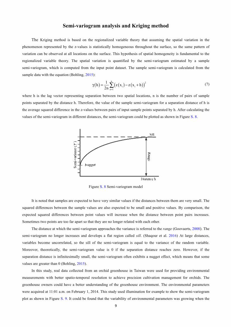
Semi-variogram analysis and Kriging method

The Kriging method is based on the regionalized variable theory that assuming the spatial variation in the

phenomenon represented by the z-values is statistically homogeneous throughout the surface, so the same pattern of

variation can be observed at all locations on the surface. This hypothesis of spatial homogeneity is fundamental to the

regionalized variable theory. The spatial variation is quantified by the semi-variogram estimated by a sample

semi-variogram, which is computed from the input point dataset. The sample semi-variogram is calculated from the

sample data with the equation (Bohling, 2015):

( ) ( ) ( )( )n 2

i in 1

1h z x z x h

2n =

γ = − +∑ (7)

where h is the lag vector representing separation between two spatial locations, n is the number of pairs of sample

points separated by the distance h. Therefore, the value of the sample semi-variogram for a separation distance of h is

the average squared difference in the z-values between pairs of input sample points separated by h. After calculating the

values of the semi-variogram in different distances, the semi-variogram could be plotted as shown in Figure S. 8.

Figure S. 8 Semi-variogram model

It is noted that samples are expected to have very similar values if the distances between them are very small. The

squared differences between the sample values are also expected to be small and positive values. By comparison, the

expected squared differences between point values will increase when the distance between point pairs increases.

Sometimes two points are too far apart so that they are no longer related with each other.

The distance at which the semi-variogram approaches the variance is referred to the range (Goovaerts, 2008). The

semi-variogram no longer increases and develops a flat region called sill. (Shaqour et al. 2016) At large distances,

variables become uncorrelated, so the sill of the semi-variogram is equal to the variance of the random variable.

Moreover, theoretically, the semi-variogram value is 0 if the separation distance reaches zero. However, if the

separation distance is infinitesimally small, the semi-variogram often exhibits a nugget effect, which means that some

values are greater than 0 (Bohling, 2015).

In this study, real data collected from an orchid greenhouse in Taiwan were used for providing environmental

measurements with better spatio-temporal resolution to achieve precision cultivation management for orchids. The

greenhouse owners could have a better understanding of the greenhouse environment. The environmental parameters

were acquired at 11:01 a.m. on February 1, 2014. This study used illumination for example to show the semi-variogram

plot as shown in Figure S. 9. It could be found that the variability of environmental parameters was growing when the

10

distance of two monitoring points h was increasing. When infinite variability approached the value 9×106, the

variability became stabilized. In this case, the corresponding distance h was about 10 m, i.e., the environmental

parameters of the monitoring site within the distance between 10 m were correlated. The correlation between

monitoring points would reduce when the distance was over 10 m. Therefore, the 10 m was chosen as the systematic

sampling of the best distance in this study. With the results, the contour map was plotted using the ordinary kriging

method.�

Figure S. 9 Semi-variograms for the illumination in the greenhouse interpolated from the measured data at 11:01 a.m.

on Feb. 1, 2014

Closing Remarks

Several possible moving paths were designed in a classroom environment to evaluate the basic performance of the

proposed algorithm in terms of successful rates of data delivery. With the results of the basic performance evaluation of

the proposed algorithm using different numbers of mobile nodes in a classroom environment, the reliability of the

propose DTCA was verified. The experimental results showed that average successful data delivery rates of the entire

tested networks with multiple mobile nodes up to 97.8% could be achieved when being employed in a classroom, even

under dense packet collision caused by the multipath effect that may occur in the test scenarios. The average successful

data delivery rates of the proposed algorithm at all locations were higher than those of the TDMA and the S-MAC. The

average energy consumed by the node (per run) when using the DCTA was also lower compared to using the S-MAC.

Moreover, the semi-variogram analysis and kriging method are used to build the contour map of the greenhouse. The

corresponding distance was about 10 m as the systematic sampling of the best distance in this study. The testing results

showed that the proposed algorithm and the designed wireless sensor network-based monitoring system were able to be

applied to the monitoring of a real orchid greenhouse.

References

Bohling, G. (2005). Introduction to geostatisticsa and variogram analysis. [Online]. Available:

http://people.ku.edu/~gbohling/ cpe940/Variograms.pdf

11

Goovaerts, P. (2008). Kriging and Semivariogram Deconvolution in the Presence of Irregular Geographical Units. Math

Geosci (40), 101–128.

Shaqour, F., Taany, R., Rimawi, O. & Saffarini, G. (2016). Quantifying specific capacity and salinity variability in

Amman Zarqa Basin, Central Jordan, using empirical statistical and geostatistical techniques. Environ Monit Assess

188(46), 1-7.