a xed point approach to model random eldsalea.impa.br/articles/v3/03-05.pdf · alea 3, 111{132...

Alea 3, 111–132 (2007)

A fixed point approach to model random fields

Paul Doukhan and Lionel Truquet

LS-CREST, Lab. Statistique, CREST Timpbre J340, 3, Avenue Pierre Larousse, 92240Malakoff and SAMOS, Statistique Appliquee et Modelisation Stochastique, UniversiteParis 1, Centre Pierre Mendes France, 90 rue de Tolbiac, F-75634 Paris Cedex 13E-mail address: [email protected]

LS-CREST, Lab. Statistique, CREST Timpbre J340, 3, Avenue Pierre Larousse, 92240Malakoff and SAMOS, Statistique Appliquee et Modelisation Stochastique, UniversiteParis 1, Centre Pierre Mendes France, 90 rue de Tolbiac, F-75634 Paris Cedex 13E-mail address: [email protected]

Abstract. We introduce new models of stationary random fields, solutions of

Xt = F((Xt−j)j∈Zd\{0}; ξt

),

the input random field ξ is stationary, e.g. ξ is independent and identically dis-tributed (iid). Such models extend most of those used in statistics. The (nontrivial)existence of such models is based on a contraction principle and Lipschitz condi-tions are needed; those assumptions imply Doukhan and Louhichi (1999)’s weakdependence conditions. In contrast to the concurrent ones, our models are not setin terms of conditional distributions. Various examples of such random fields areconsidered. We also use a very weak notion of causality of independent interest: itallows to relax the boundedness assumption of inputs for several new heteroscedas-tic models, solutions of a nonlinear equation.

1. Introduction

Description of random fields is a difficult task, a very deep reference is Georgii’s1988 book; a synthetic presentation is given by Follmer (1988). The usual way todescribe interactions makes use of conditional distributions with respect to largesets of indices. This presentation is natural for discrete valued random fields asin Comets et al. (2002). The existence of conditional densities is a more restrictiveassumption for continuous state spaces. The existence of random fields is oftenbased on conditional specifications, see Follmer (1988, pages 109–119) and Do-brushin (1970), through Feller continuity assumptions. The uniqueness of Gibbs

Received by the editors January 9 2007; accepted July 14 2007.

2000 Mathematics Subject Classification. 60G60, 60B12, 60F25, 60K35, 62M40, 60B99, 60K99.Key words and phrases. Random fields, Limit theorems for vector-valued random variables,

Lp-limit theorems, Interacting random processes; statistical mechanics type models; percolationtheory, Random fields; image analysis, Weak dependence, Bernoulli shifts.

111

112 Paul Doukhan and Lionel Truquet

measures is often based on projective conditional arguments; it follows with a mix-ing type argument. Such conditions rely on the regularity of conditional distri-butions; applications to resampling exclude such hypotheses. Various applicationsto image, geography, agronomy, physic, astronomy or electromagnetism may forinstance be considered, see Georgii (1988) or Loubaton (1989).We omit here any assumption relative to the conditional distributions. Our idea isto define random fields through more algebraic and analytic arguments. We presenthere the new models of stationary random fields subject to the relation:


)(1)

where ξ = (ξt)t∈Zd is an independent identically distributed (iid) random field. Theindependence of inputs ξ may also be relaxed to a stationarity assumption.For the models with infinite interactions (1), the existence and uniqueness relyon the contraction principle. Lipschitz type conditions are thus needed, they areclosely related to weak dependence, see Doukhan and Louhichi (1999). Analogueweak dependence conditions are already proved in Shashkin (2005) for spin systems.A causal version of such models, random processes solutions of an equation Xt =F (Xt−1, Xt−2, . . . ; ξt) (t ∈ Z) is considered in Doukhan and Wintenberger (2006);in this paper the results are proved in a completely different way fitting to couplingarguments. Our results state existence and uniqueness of a solution of (1) as aBernoulli shift Xt = H((ξt−s)s∈Zd) as well as the weak dependence properties ofthis solution.Our models are not necessarily Markov, neither linear or homoskedastic. Moreoverthe inputs do not need additional distributional assumptions (like for Gibbs randomfields). They extend on ARMA random fields which are special linear randomfields (see Loubaton (1989) or Guyon (1995)). A forthcoming paper will be aimedat developing statistical issues of those models. Identification and estimation ofrandom fields with integer values will be considered in Doukhan et al. (2007).The paper is organized as follows. We first recall weak dependence from Doukhanand Louhichi (1999) in § 2. General results are then stated for stationary (nonnecessarily independent) inputs. Those results imply heavy restrictions on theinnovations in some cases: a convenient notion of causality is thus used. A lastsubsection addresses the problem of simulating such models.A following section details examples of such models. They are natural extensionsof the standard times series models. We shall especially consider LARCH(∞) anddoubly stochastic linear random fields for which this causality allows to relax theboundedness assumptions. Proofs are postponed to a last section of the paper.

2. Main results

In order to state our dependence results, we first introduce the concepts of weakdependence. Our main results will be stated in the following subsection. After this,causality will be proved to imply other powerful results. A last subsection is aimedat describing a way to simulate those very general random fields.

2.1. Weak dependence. We recall here the weak dependence conditions introducedin Doukhan and Louhichi (1999). They may replace heavy mixing assumptions.

Definition 1. Set ‖(s1, . . . , sd)‖ = max{|s1|, . . . , |sd|} for s1, . . . , sd ∈ Z. One E =R

k−valued random field (Xt)t∈Zd is weakly dependent if for a sequence (ε(r))r∈N

A fixed point approach to model random fields 113

with limit 0

|Cov (f(Xs1, . . . , Xsu

) , g (Xt1 , . . . , Xtv)| ≤ ψ(u, v,Lip f,Lip g)ε(r),

where indices s1, . . . , su, t1, . . . , tv ∈ Zd are such that ‖sk − tl‖ ≥ r for 1 ≤ k ≤ u

and 1 ≤ l ≤ v. Moreover, the real valued functions f, g defined on(R

k)u

and(R

k)v

, satisfy ‖f‖∞, ‖g‖∞ ≤ 1 and Lip f,Lip g < ∞ where a norm ‖ · ‖ is given

on Rk and,

Lip f = sup(x1,...,xu)6=(y1,...,yu)

|f(x1, . . . , xu) − f(y1, . . . , yu)|‖x1 − y1‖ + · · · + ‖xu − yu‖

.

If ψ(u, v, a, b) = au + vb, this is denoted as η−dependence and the sequence ε(r)will be written η(r).If ψ(u, v, a, b) = abuv, this is denoted as κ−dependence and the sequence ε(r) willbe written κ(r).If ψ(u, v, a, b) = au+ vb+abuv, this is denoted as λ−dependence and the sequenceε(r) will be written λ(r).

2.2. Random fields with infinite interactions. Let ξ = (ξt)t∈Zd be a stationary ran-

dom field with values in E′ (usually E′ = Rk′

for some k′ ≥ 1 but in some cases E ′

is a denumerable tensor product of such sets). We shall consider stationary E = Rk

valued random fields driven by the implicit equation (1). For a topological spaceS, B(S) denote the Borel σ-algebra on S.We denote I = Z

d \{0}. In the sequel, F :(E(I)×E′,B(EI)⊗B(E′)

)→(E,B(E)

)

denotes a measurable function defined for each sequence with a finite number ofnon-vanishing arguments (1). In this paper ‖ · ‖ will be arbitrary norms on E (orE′ when needed). We will always use the suppremum norm on Z

d and this normwill be also denoted by ‖ · ‖. We prove that simple assumptions entail existence ofa unique solution as a Bernoulli shift

Xt = H((ξt−j)j∈Zd

)

Let µ denote ξ’s distribution; this is a probability measure on the measurable space(E′Zd

,B(E′Zd))

. For some m ≥ 1, we denote ‖ · ‖m the usual norm of Lm and

the space of µ-measurable H :(E′Zd

,B(E′Zd))

→ (E,B(E)) with finite momentsis denoted

Lm(µ) = {H

/E‖H(ξ)‖m <∞}.

We shall use the assumptions:

: (H1) ‖F (0; ξ0)‖m <∞.: (H2) There exist constants aj ≥ 0, for j ∈ α > 0 with, for each ∀z, z′ ∈E(Zd\{0}),

‖F (z; ξ0) − F (z′; ξ0)‖ ≤∑

j∈Zd\{0}aj‖zj − z′j‖, a.s. (1)

∑

j∈Zd\{0}aj = e−α < 1.

We now extend the function F to the trajectories of a stationary random field:

1If V denotes a vector space and B an arbitrary set then V (B)⊂ V B denotes the set of

v = (vb)b∈B such that there is some finite subset B1 ⊂ B with vb = 0 for each b /∈ B1.


Lemma 1. Assume (H1) and (H2). Let X and X ′ be two E−valued stationnaryrandom fields in L

m, then:

1) limp→∞

F((Xj10<‖j‖≤p)j 6=0; ξ0

)exists in L

m and a.s., we denote it

F((Xj)j∈Zd\{0}; ξ0

).

2)∥∥F((Xj)j∈Zd\{0}; ξ0

)− F

((X ′

j)j∈Zd\{0}; ξ0)∥∥

m≤

∑

j∈Zd\{0}aj

∥∥Xj −X ′j

∥∥m.

Theorem 1. Assume that ξ is stationary and (H1) and (H2) hold. Then thereexists a unique stationary solution of equation (1). This solution writes Xt =H((ξt−j)j∈Zd

)for some H ∈ L

m(µ).

Lemma 8 below, will also provide us with an approximation of this solution withfinitely many interactions.

2.2.1. Weak dependence of the solution (iid inputs). In the general case we shallrestrict to independent inputs to derive η−weak dependence of the previous solu-tion.

Theorem 2. Assume that ξ is iid and (H1) and (H2) hold. Then the stationarysolution of equation (1) obtained in theorem 1 is η−weakly dependent and thereexists a constant C > 0 with

η(r) ≤ C · infp∈N∗

{e−α r

2p +∑

‖i‖>p

ai

}. (2)

Remark. If ai = 0 for ‖i‖ > p then η(r) ≤ C · e−α r2p .

Sub-geometric rates are now derived from specific decays of the coefficients:

Lemma 2 (Geometric decays). If ai ≤ Ce−β‖i‖ there exists a constant C ′ > 0 with

η(r) ≤ C ′rd−1

2 e−√

αβr/2.

Lemma 3 (Riemanian decays). If ai ≤ C‖i‖−β for a β > d, there exists C ′ > 0with

η(r) ≤ C ′( r

ln r

)d−β

.

Thus a large range of decay rates may be considered for such models of randomfields.

2.2.2. Weak dependence of the solution (dependent inputs). If ξ is either η or λ-dependent it may be proved in specific examples that weak dependence is hereditary.Here follows a general result. The following assumption will be necessary:

(H2’) There exist a subset Ξ ⊂ E ′ with P (ξ0 ∈ Ξ) = 1, nonnegative constants with∑

j∈Zd\{0}aj = e−α < 1 and a constant b > 0 such that

‖F (x;u) − F (x′;u′)‖ ≤∑

j∈Zd\{0}aj‖xj − x′j‖ + b ‖u− u′‖ ,

for all x, x′ ∈ E(Zd\{0}) and u, u′ ∈ Ξ.

We quote that assumption (H2’) is more restrictive than (H2)


Proposition 1. Assume (H1) and (H2’).

1): If the random field ξ is η−weakly dependent, with weak dependencecoefficients ηξ(r), then X is η−weakly dependent with, for some C > 0,

η(r) ≤ C infp∈N∗

{ ∑

‖j‖>p

aj + infn∈N∗

{an + pnηξ ((r − 2pn) ∨ 0)

}}.

2): If the random field ξ is λ−weakly dependent, with dependence coefficientsdenoted λξ(r), then X is λ−weakly dependent with, for some C > 0,

λ(r) ≤ C infp∈N∗

∑

‖j‖>p

aj + infn∈N∗

{an + p2nλξ ((r − 2pn) ∨ 0)

} .

Remark. For models with finite interactions, i.e. F (x;u) = f(xj1 , . . . , xjk;u) for

x = (xj)j 6=0, this simply writes

η(r) ≤ c infn∈N∗

{an + knηξ ((r − 2ρn) ∨ 0)} ,

λ(r) ≤ c infn∈N∗

{an + k2nλξ ((r − 2ρn) ∨ 0)

},

here ρ = max{‖j1‖, . . . , ‖jk‖}. If ηξ(r) or λξ(r) have geometric or Riemanniandecay the same holds for the output random field. More precisely set a = e−α andk = eκ under η-dependence and k2 = eκ under λ-dependence, then decay rates ofthe outputs (Xt) writeGeometric decays:

eαβ

α+2ρβ+κr for dependence decays of the inputs with order e−βr

Riemannian decays:

r−αb

α+κ for dependence decays of the inputs with order r−b

2.3. Causality. For d = 1, the recurrence equation Xt = ξt(a+bXt−1) is given withF (x;u) = u(a+ bx1). There exist a stationary solution with ξt and Xt−1 indepen-dent. Here (H2) implies that innovations are bounded, which seems unrealistic.In this example, instead of H ((ξt)t∈Z)) ∈ L

m(µ), this is enough to exhibit solu-tions H ((ξt)t≥0) ∈ L

m(µ) (which is independent of (ξs)s<0). This allows to replacesuprema by integrals in (H2) in order to derive a contraction principle. Causalityof random fields has been considered in Helson and Lowdenslager (1959); we adaptthis idea in order to relax the previous assumption.

Definition 2 (causality). If A ⊂ Zd \ {0}, we denote c(A) the convex cone of R

d

generated by A,

c(A) =

{k∑

i=1

riji

/(j1, . . . , jk) ∈ Ak, (r1, . . . , rk) ∈ R

k+, k ≥ 1

}.

1) The set A is a causal subset of Zd if c(A) ∩

(− c(A)

)= {0}.

2) If F is measurable with respect to the σ-algebra FA ⊗B(E′) for some causal setA, then the equation Xt = F ((Xt−j)j∈I ; ξt) is A-causal.

For a causal set A ⊂ Zd, we denote by A the subset c(A) ∩ Z

d.


Examples. A singleton is causal, as well as {i, j} if and only if −j /∈ i · R+. The

half plane {(i, j) ∈ Z2/i > 0}

⋃{(0, j); j > 0} ⊂ Z

2 is also causal.

One consequence of this notion is the elementary lemma:

Lemma 4. If A is a causal subset of Zd, then ∀(j, j′) ∈ A× A we have j + j′ 6= 0.

For a linear basis b = (b1, . . . , bd) of Rd, (x1, . . . , xd) 7→ x1b1 + · · ·+xdbd, defines

an isomorphism f : Rd → R

d. We denote by ≤b the total order relation on Rd

defined by:u ≤b v ⇔ f−1(u) ≤lex f

−1(v)

with ≤lex the lexicographic order on Rd.

Proposition 2 (characterization of causal sets). If B is a convex cone of Rd such

that B ∩ (−B) = {0} there exists a basis b of Rd such that B ⊂ {j ∈ R

d/0 ≤b j}.Moreover if b is a basis of R

d, {j ∈ Zd/0 <b j} is a causal set of Z

d witch will becalled maximal causal subset.

Remarks.

• The maximal causal subsets of Z are {1, 2, 3, . . .} and {−1,−2, . . .}. Anexample of maximal causal subset of Z

2 is {(i, j) ∈ Z2/i > 0 or (i = 0, j >

0)}.• Helson and Lowdenslager (1959) define symmetric half planes as subsetsS ⊂ Z

2 such that S is stable by addition and S ∪ (−S) = Z2, S ∩ (−S) =

{0}. A nice review of this causality condition is given in Loubaton (1989),applications are essentially given in terms of linear random fields.

Note that S \ {0} is a maximal causal subset of Z2. This notion plays a

prominent part in prediction theory of 2-D stationary process (see Loubaton(1989)).

If D ⊂ Zd, we denote by πs (respectively π′

s) the coordinate applications in EZd

(resp. in (E′)Zd

), FD = σ(πs; s ∈ D) and F′D = σ(π′

s; s ∈ D). Hence we denoteby L

mD(µ) the subspace of L

m(µ) of functions µ-measurable with respect to F′D.

The following result takes this definition into account to relax the assumptions intheorem 1,

Theorem 3. Let Xt = F((Xt−j)j∈Zd\{0}; ξt

)be a A-causal equation with iid inputs

ξ. Besides the assumption (H1) we assume the following condition:(H3) there exist nonnegative constants with

∑j∈A aj = e−α < 1 and

‖F (x; ξ0) − F (x′; ξ0)‖m ≤∑

j∈A

aj‖xj − x′j‖, ∀x, x′ ∈ E(Zd\{0}).

Then there exists a unique strictly stationary solution X of this equation in Lm if

for each t ∈ Zd, Xt is measurable wrt σ

(ξt−j/j ∈ A

).

This solution writes Xt = H((ξt−j)j∈Zd

)where H ∈ L

meA . and it is η−weakly

dependent; moreover relation (2) still holds for a constant C > 0.

Now the function F is extended as follows:

Lemma 5. Suppose (H1) and (H3). If ξ0 is independent of σ((Xj , X

′j)/j ∈ A

)for

two random fields X and X ′ in Lm then,

1) limp→∞

F((Xj10<‖j‖≤p)j 6=0; ξ0

)exists in L

m and it is denoted F((Xj)j 6=0; ξ0

).


2)∥∥F((Xj)j 6=0; ξ0

)− F

((X ′

j)j 6=0; ξ0)∥∥

m≤∑

j∈A

aj

∥∥Xj −X ′j

∥∥m

.

2.4. Simulation of the model. Simulations of those models are deduced from theproof of the existence theorems based on the Picard fixed point theorem. Consider

the shift operators θj :(E′)Z

d

→(E′)Zd

defined as (xk)k∈Zd 7→ (xk+j )k∈Zd . ForH ∈ L

m(µ) we note

Φp(H) = F((

(H ◦ θj)1‖j‖≤p

)j;π0

)

It is shown in theorem 1’s proof that the application Φ : Lm(µ) → L

m(µ) given by

Φ(H) = F ((H ◦ θj)j 6=0;π0).

is well defined and has a fixed point in Lm(µ).

The proof of theorem 3 shows that it is also the case for a A−causal equation if wereplace L

m(µ) by LmeA (µ).

For n, p ∈ N∗, t ∈ Z

d we denote

Xnt = Φ(n)(0)

((ξt−j)j∈Zd

)

and

Xnp,t = Φ(n)

p (0)((ξt−j)j∈Zd

).

Lemma 6. We assume that conditions in theorem 1 or in theorem 3 hold for somem ≥ 1. Let n ∈ N then:

(1) For every t ∈ Zd, ‖Xt −Xn

t ‖m ≤ an‖X0‖m, hence limn→∞Xnt = Xt a.s.

(2) if p ∈ N we have,∥∥Xt −Xn

p,t

∥∥m

≤ ‖X0‖m

{an + 1

1−a

∑‖j‖>p aj

}. Thus if

p = pn is chosen such that∑

n≥1

( ∑

‖j‖>pn

aj

)m

<∞ then

limn→∞

Xnpn,t = Xt, a.s. (3)

Remarks.

• If the random field has finitely many interactions, then 1. provides a sim-ulation scheme.

• For each finite p the operator Φp can be calculated thus relation (3) providesan explicit simulation scheme even for infinitely many interactions.

• A.s. convergence rates may also be evaluated in the previous lemma. Theywrite oa.s. (a

nnε) in the first point for each ε > 1/m and oa.s. (n−ε) for

0 < ε < α − 1/m if∑

‖j‖>pnaj ≤ Cn−α for some C > 0, α > 1/m in the

point 2.• If T ⊂ Z

d is a finite set the random field X may be analogously simulatedover T and (Xt)t∈T is estimated by

(Xn

pn,t

)t∈T

.

2.4.1. Simulation scheme for finitely many interactions. Let

F (x;u) = f(xj1 , . . . , xjk;u).

The sequence of random fields Xn is defined from:

X1t = f(0; ξt), t ∈ Z

d, Xn+1t = f

(Xn

t−j1 , . . . , Xnt−jk

; ξt), for n ≥ 0


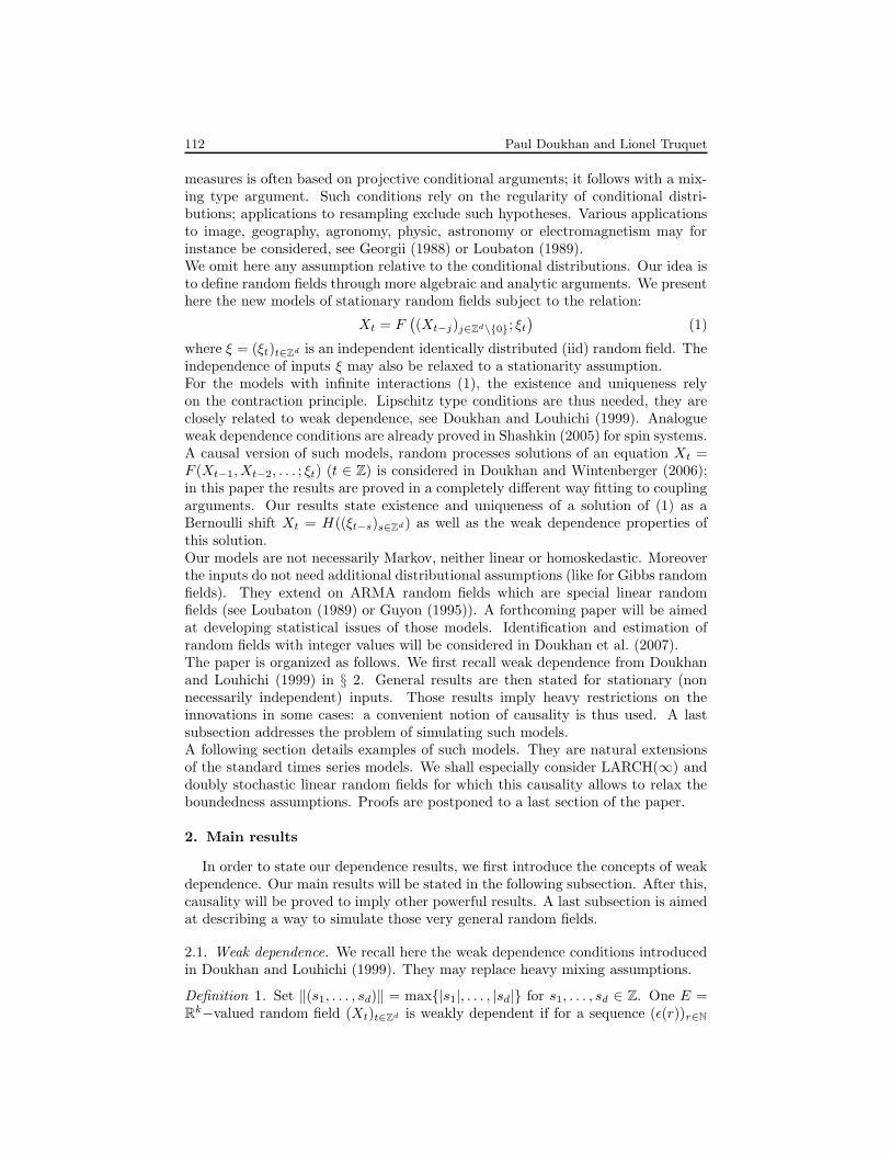
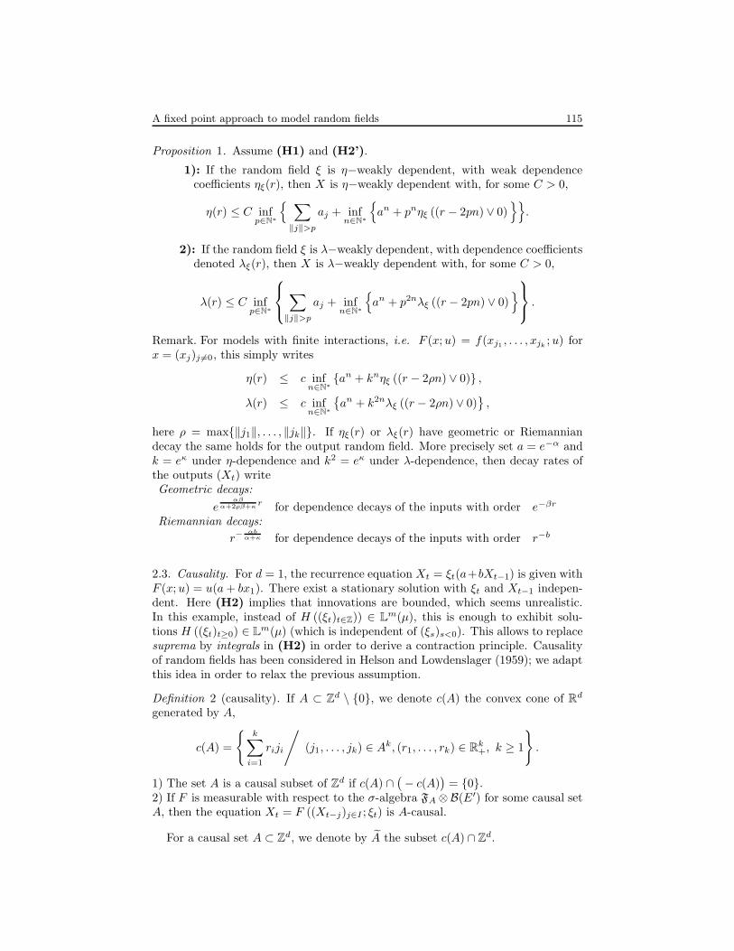
We now simulate samples (X10t )1≤t1,t2≤15 of LARCH models with d = 2, k = k′ = 1

and p = 10:

Xt = ξt

(1 +

∑

0<‖j‖≤p

ajXt−j

)

(1) In the figure 1, we represent the non causal case with aj =0.05

j21 + j22and ξ0

is uniform on [−1, 1].

(2) Figure 2 deals with the causal case with aj =0.05

j21 + j22if 0 ≤ j1, j2 ≤ 10 and

aj = 0 otherwise. In this case, ξ0 is N(0, 1)-distributed.

Figure 1. Non causal LARCH field.

Figure 2. Causal LARCH field.


3. Examples

Theorems 2 and 3 are now applied to examples of random fields with infiniteinteractions. Causality will allow to weaken moment conditions. In fact, theorem2 proves a contraction principle in L

m for each value of m while theorem 3 onlyworks with one fixed value of m.

3.1. Finite interactions random fields. If ξt = (ζt, γt) with ζt ∈ Rp and γt a p × q

matrix, and functions f(·) ∈ Rp and g(·) ∈ R

q

Xt = f(Xt−`1 , . . . , Xt−`k) + γtg(Xt−`1 , . . . , Xt−`k

) + ζt (1)

with `1, . . . , `k 6= 0.E.g. non linear auto-regression corresponds to γt ≡ 0 and ARCH type models areobtained with ζt = 0 (classically p = q = 1, f is linear and g2(x1, . . . , xk) is anaffine function of x2

1, . . . , x2k).

Theorems 1, 2, 3 imply the following lemma,

Corollary 1. Suppose ‖ζ0‖m <∞ and{

‖f(x1, . . . , xk) − f(y1, . . . , yk)‖ ≤ ∑ki=1 bi‖xi − yi‖,

‖g(x1, . . . , xk) − g(y1, . . . , yk)‖ ≤ ∑kj=1 cj‖xj − yj‖

.

(1) If ξ is iid and

k∑

i=1

(bi + ‖γ0‖∞ci

)= e−α < 1, then η(r) ≤ C

(e−

α2k

)rfor

model (1).

If the equation (1) is causal andk∑

i=1

(bi + ‖γ0‖mci

)= e−α < 1, the same

holds.

(2) If now ξ is η or λ-weakly dependent, g bounded and

k∑

i=1

(bi + ‖γ0‖∞ci

)=

e−α < 1, then X is η or λ-weakly dependent. Decays are given accordingto proposition 1.

The remark following proposition 1 states precise decays. The volatility coeffi-cients γt need to be bounded in the general case and they only have finite momentsunder causality. Functions f and g may only depend on a strict subset of the indices1, . . . , k.

3.2. Linear fields. Let X be a solution of the equation

Xt =∑

j∈A

αjtXt−j + ζt, (2)

innovations ζt are vectors of E = Rk and coefficients αj

t are k × k matrices, ‖ · ‖ isa norm of algebra on this set of matrices and X will be an E valued random field.

Let A ⊂ Zd \ {0}, we assume that the iid random field ξ =

((αj

t )i∈A, ζt

)

t∈Zdtakes

now its values in (Mk×k)A × E; here Mk×k denotes the set of k × k matrices.


Proposition 3. If b =∑

j∈A ‖αj0‖∞ < 1, then theorem 2 applies with aj = ‖αj

0‖∞.

For a causal equation if b =∑

j∈A ‖αj0‖m < 1 theorem 3 applies with aj = ‖αj

0‖m.

In both cases the solution of equation (2) writes a.s. and in Lm,

Xt = ζt +∑

j∈A

αjtξt−j +

∞∑

i=2

∑

j1,...,ji∈A

αj1t α

j2t−j1

· · ·αji

t−j1−···−ji−1ζt−(j1+···+ji).

This means that the random coefficients are bounded in the general case andthey need only to have have finite moments under causality.Examples. If the sequence (αj

t )t is deterministic then those models extend on linear

auto-regressive models. If only a finite number of coefficients αjt do not vanish we

obtain auto-regressive models with random coefficients, see Tjostheim (1986).

3.3. LARCH(∞) random fields. Stationary innovations ξt are now k × k′ matricesand ‖ · ‖ will denote a norm k × k′ or k′ × k matrices while Xt ∈ R

k. For boundedinnovations we first recall

Theorem 4 (Doukhan, Teyssiere, Winant (2006)). Let αj be a k′ × k matrix forj ∈ Z

d \{0}, note A(x) =∑

‖j‖≥x ‖αj‖ and suppose that λ = A(1)‖ξ0‖∞ < 1, then

Xt = ξt

a+

∞∑

k=1

∑

j1,...,jk 6=0

αj1ξt−j1 · · ·αjkξt−j1−···−jk

a

(3)

is a solution of the equation

Xt = ξt

a+∑

j 6=0

αjXt−j

, t ∈ Zd (4)

if moreover ξ is iid, then

η(r) ≤ E‖ξ0‖

E‖ξ0‖

∑

k<r/2

λk−1A( rk

)+λ[r/2]

1 − λ

‖a‖.

If we use theorem 2 we also obtain that eqn. (4) admits a unique Bernoullishift L

m solution. Note that this solution is bounded. Notice that for Riemanniandecay the previous A(u) ≤ Cu−c relation yields η(r) = O(r−c) while theorem 3only provides us this bound up to a log-loss; geometric decays yield the same resultfor both cases.Bounded innovations ξt look unnatural hence we investigate below the causal case.Let A a causal subset of Z

d and

Xt = ξt

(a+

∑

s∈A

asXt−s

)(5)

Proposition 4. If b‖ξ0‖m < 1 with b =∑

s∈A ‖as‖, theorem 3 applies with aj =‖ξ0‖m‖αj‖ to the solution (3) of eqn. (5) (we set αj = 0 for j /∈ A).


3.4. Non linear ARCH(∞) random fields. Models with

Xt = ξt

(a+

∑

j 6=0

gj(Xt−j))

clearly extend on LARCH(∞) models; bounded functions gj provide robust models.

Corollary 2. If ‖gj(x) − gj(y)‖ ≤ αj‖x − y‖ and ‖ξ0‖∞∑

j 6=0 αj < 1, theorem 2

holds with ai = ‖ξ0‖∞αi (innovations are bounded here).Assume now that gi ≡ 0 for i /∈ A, causal set then theorem 3 holds with ai =‖ξ0‖mαi (and now the innovations do not need anymore to be bounded).

This causality argument improves on Doukhan et al. (2006) by only assumingfinite moments for innovations instead of boundedness.

3.5. Mean field type model. Consider innovations in Rk′

and k × k matrices αi,

Xt = f(ξt,∑

s6=t

αs−tXs

)(6)

Corollary 3. Assume that f : Rk′ × R

k → Rk satisfies

supu∈Rk′

‖f(u, x) − f(u, y)‖ ≤ b‖x− y‖, ∀x, y ∈ Rk, b

∑

i6=0

‖αi‖ < 1.

then equation (6) admits a unique solution in Lm written as a Bernoulli shift and

this solution is η−weakly dependent with ai = b‖αi‖1.The same results hold if now ai = 0 for i /∈ A with A is causal in Z

d and,∥∥f(ξ0, x)

)− f

(ξ0, y

)∥∥m

≤ b‖x− y‖, ∀x, y ∈ Rk, b

∑

i6=0

‖αi‖ < 1.

LARCH(∞) models take this form.

4. Proofs

We begin with the proof of some lemmas which relate the assumptions to con-traction conditions in the space of Bernoulli shifts. Then we give separated proofsfor existence and weak dependence properties. Those proofs always follow twosteps since we first consider models with a finite range. For shortness we write hereI = Z

d \ {0}.

4.1. Proof of lemma 1. For p ∈ N∗, we set Yp = F

((Xj10<‖t‖≤p)j , ξ0

)and Y ′

p =

F((X ′

j10<‖t‖≤p)j , ξ0).

(1) If q ∈ N∗ from assumption (H2),

‖Yp − Yp+q‖ ≤∑

p<‖j‖≤p+q

aj ‖Xj‖ , a.s.

Since the serie∑

j∈I aj ‖Xj‖m is convergent the serie∑

j∈I aj ‖Xj‖ con-

verges a.s. Hence, we deduce that a.s (Yp)p∈N∗ is a Cauchy sequence in Eand then converges. We denote by Y = F

((Xj)j 6=0; ξ0

)this limit.

Moreover, for p ∈ N∗, we have:

‖Yp − F (0; ξ0)‖m ≤∑

0<‖j‖≤p

aj ‖Xj‖m


This proves that Yp ∈ Lm. Hence the convergence in L

m is a simplyconsequence of the Fatou lemma since:

‖Y − Yp‖m ≤ lim infq→∞

‖Yq − Yp‖m ≤∑

‖j‖>p

aj ‖X0‖m

(2) If p ∈ N∗, we have using (H2):

∥∥Yp − Y ′p

∥∥m

≤∑

j 6=0

aj

∥∥Xj −X ′j

∥∥m

,

hence the result follows with p→ ∞. �

4.2. Proof of the existence theorem 1. Assuming (H1) and (H2) we set a =∑j 6=0 aj . With the notations of paragraph 2.4.,

Φp(H) = F((

(H ◦ θj)1‖j‖≤p

)j;π0

), ∀H ∈ L

m(µ)

As a direct consequence of lemma 1, limp→∞ Φp(H) exists in Lm(µ). Denote this

limit by F ((H ◦ θj)j 6=0;π0), the application Φ : Lm(µ) → L

m(µ) is defined as

Φ(H) = F ((H ◦ θj)j 6=0;π0) .

Let show that Φ is a contraction of Lm(µ).If H , H ′ ∈ L

m(µ), then applying thelemma 1 to the random fields X and X ′ defined as Xj = H ◦ θj(ξ) and X ′

j =H ′ ◦ θj(ξ), we obtain:

‖Φ(H)(ξ) − Φ(H ′)(ξ)‖m ≤∑

j 6=0

aj‖H ◦ θj(ξ) −H ′ ◦ θj(ξ)‖m

≤∑

j 6=0

aj‖H(ξ) −H ′(ξ)‖m

Picard fixed point theorem applies since the space Lm(µ) is complete. There exists

a unique H ∈ Lm(µ) with Φ(H) = H thus H(ξ) = F

((H ◦ θj(ξ))j∈Zd ; ξ0

), a.s. Set

Xt = H ((ξt−i)i∈Zd) then with stationarity of ξ and since Zd is denumerable we get


), ∀t ∈ Z

d a.s.

Let Y be a stationary solution of this equation, we denote ut = ‖Xt − Yt‖1 foreach t ∈ Z

d. We obtain ut ≤ ∑j 6=0 ajut−j . As supt ut ≤ ‖X0‖1 + ‖Y0‖1 < ∞ we

note that the previous relation implies supt ut ≤ a supt ut. Hence ut = 0 for eacht. Thus Xt = Yt a.s for each t. �

4.3. Proof of theorem 2. For an independent copy (ξ ′t)t∈Zd of ξ = (ξt)t∈Zd and

s ∈ R+, we set ξ(s) = (ξ

(s)t )t∈Zd with ξ

(s)t = ξt if ‖t‖ < s and ξ

(s)s = ξ′s else. For

a Bernoulli shift defined by H a straightforward extension of a result in Doukhanand Louhichi (1999) to random fields implies

η(r) ≤ 2δr/2, where δr =∥∥∥H (ξ) −H

(ξ(r))∥∥∥

1(1)


4.3.1. Weak dependence under finite interactions. We first assume that F dependsfinitely many variables

Xt = F (Xt−j1 , . . . , Xt−jk; ξ0)

Lipschitz coefficients of F in condition (H2) write a1, . . . , ak and we set a =∑ki=1 ai < 1 and ρ = max{‖j1‖, . . . , ‖jk‖}. Let H be the element of L

m(µ)

with Xt = H ((ξt−i)i∈Zd) and δr = E∥∥H(ξ) −H(ξ(r))

∥∥ = E

∥∥∥X0 −X(r)0

∥∥∥ with

X(r)t = H((ξ

(r)t−i)i∈ Zd).

Lemma 7. Assume that (H1) and (H2) hold, then δr ≤ 2‖X0‖1arρ hence δr →r→∞

0.

Proof of lemma 7. Let r > 0. Since ξ and ξ(r) admit the same distribution, we havefor each t:

Xt = F (Xt−j1 , . . . , Xt−jk; ξt), X

(r)t = F (X

(r)t−j1

, . . . , X(r)t−jk

; ξ(r)t )

If ‖t‖ < r then ξ(r)t = ξt and using (H2), we have:

‖Xt −X(r)t ‖1 ≤

k∑

l=1

al

∥∥∥Xt−jl−X

(r)t−jl

∥∥∥1

(2)

Set now i = −[− rρ ] if r ≥ ρ, then if u ≤ i− 1 and l1, . . . , lu ∈ {1, . . . , k}: ‖jl1 +

jl2 + · · · + jlu‖ < r. We use inequality (2) to derive recursively the bounds

∥∥∥X0 −X(r)0

∥∥∥1≤

k∑

l1=1

al1

k∑

l2=1

al2 · · ·k∑

li=1

ali

∥∥∥X−(jl1+jl2

+···+jli) −X

(r)−(jl1

+jl2+···+jli

)

∥∥∥1

≤ 2‖X0‖1ai

From i ≥ r/ρ we get ‖X0 −X(r)0 ‖1 ≤ 2‖X0‖1 a

rρ thus δr ≤ 2‖X0‖1a

rρ .

If now r < ρ,∥∥∥X0 −X

(r)0

∥∥∥1≤∑k

l1=1 al1

∥∥∥X−jl1−X

(r)−jl1

∥∥∥1.

Thus δr ≤ 2‖X0‖1ai ≤ 2‖X0‖1 a

rρ . The result follows with a < 1. �

We now set a useful result. (Xt)t∈Zd and (Xp,t)t∈Zd will denote for p ≥ 0 the previ-ous unique solution of the equations (1) and Zt = F

((Zt−j1{0<‖j‖≤p})j∈Zd\{0}; ξt

).

Lemma 8. Assume that the conditions in theorem 1 hold. Then Xp,t →s→∞ Xt inL

m, for each t ∈ Zd.

Proof. ‖Xp,0−X0‖m ≤ a‖Xp,0−X0‖m +‖X0‖m

∑

‖j‖>p

aj , thus ‖Xp,0−X0‖m ≤P

‖j‖>p aj

1−a ‖X0‖m which entails the first result. We also quote that supp ‖Xp,0‖m <∞. �

4.3.2. Weak dependence.

Lemma 9. Assume that the conditions in theorem 1 hold. Then the random field(Xt)t∈Zd is η-weakly dependent.


Proof. Recall that supp ‖Xp,0‖m <∞; if m ≥ 1, weak dependence follows from

E‖X(r)0 −X0‖ ≤ E‖X(r)

0 −X(r)p,0‖ + E‖X(r)

p,0 −Xp,0‖+ E‖Xp,0 −X0‖= 2E‖Xp,0 −X0‖ + E‖X(r)

p,0 −Xp,0‖

For r ≥ p, from lemma 7 we derive E‖X (r)p,0 −Xp,0‖ ≤ 2‖Xp,0‖1

( ∑

‖j‖≤p

aj

) rp

. Hence

δr = E‖X(r)0 −X0‖ ≤ 2 · ‖X0‖1

1−a

∑‖j‖>p aj + 2‖Xp,0‖1 a

rp .

With supp ‖Xp,0‖1 < ∞ there exists C > 0 with δr ≤ C · infp

{∑‖j‖>p aj + a

rp

}.

Using (1) we prove that (Xt)t is η-weakly dependent and η(r) ≤ δr/2. �

4.3.3. Decay rates. Using the representation of the solution as a Bernoulli shiftand the inequality (1) this will be enough to bound the expression of δr. Setbp = #{i ∈ Z

d/ ‖i‖ ≤ p} and sp = #{i ∈ Zd/ ‖i‖ = p} for ‖i‖ = max{|i1|, . . . , |id|}

we obtain bp = (2p+ 1)d and sp = bp − bp−1 ≤ Kpd−1 for a constant K > 0.

Proof of lemma 2.∑

‖j‖>p

aj =∑

q>p

∑

‖j‖=q

e−βq ≤ Kpd−1∑

q>p

e−βq = O(pd−1e−βp

).

We thus find a constant C1 such that

δr ≤ C1 infp

{pd−1e−βp + e−α r

p

}= C1 inf

p

{e−βp+(d−1) ln p + e−α r

p

}.

Assume p ∼√αr/β, there is a constant C2 such that: δr ≤ C2r

d−1

2 e−√

αβr. �

Proof of lemma 3. As before,∑

‖j‖>p aj ≤ K pd−β

β−d . Hence

δr ≤ c · infp

{e−αr/p +

pd−β

β − d

}.

Choose p ∼ αr(β−d)lnr , thus there exists some constant C3 with δr ≤ C3

(r

ln r

)d−β.

�

4.4. Proof of proposition 1.

4.4.1. Models with finite interactions. We assume first that there exist k ≥ 1 andj1, . . . , jk ∈ I such F (x;u) only depends on xj1 , . . . , xjk

for each x = (xj)j 6=0 ∈ EI .Hence writing ai instead of aji

for 1 ≤ i ≤ k, we have

‖F (x;u) − F (y;u′)‖ ≤k∑

i=1

ai‖xji− yji

‖ + b‖u− u′‖, a =k∑

i=1

ai < 1

Now h : Ek × E′ → E is such that F (x;u) = h(xj1 , . . . , xjk, u). We will denote

ρ = max{‖j1‖, . . . , ‖jk‖}.

Lemma 10. 1) If the random field ξ is η−weakly dependent (the weak dependencecoefficients are denoted ηξ(r)) then X is η−weakly dependent with, for C > 0,

η(r) ≤ C infn∈N∗

{an + knηξ ((r − 2ρn) ∨ 0)

}


2) If the random field ξ is λ−weakly dependent (the weak dependence coefficientsare denoted λξ(r)) then X is λ−weakly dependent, for C > 0,

λ(r) ≤ C infn∈N∗

{an + k2nλξ ((r − 2ρn) ∨ 0)

}

Proof of lemma 10. We will use the lemma 6 and the following useful lemma 11.

Lemma 11. (1) For every x and y ∈ C(Zd) we have ‖Φ(0)(x) − Φ(0)(y)‖ ≤b‖x0 − y0‖ and if n ≥ 2,

‖Φ(n)(0)(x) − Φ(n)(0)(y)‖

≤n−1∑

l=1

k∑

i1,...,il=1

ai1 · · · ailb‖xji1

+···+jil− yji1

+···+jil‖ + b‖x0 − y0‖

(2) Fix x ∈ C(Zd). Then Φ(0)(x) only depends on x0 and Φ(0) defines ab−Lipschitz function on C. We set K1 = b and p1 = 1.For n ≥ 2 we set An =

⋃n−1l=1 {ji1 + · · · + jil

/ 1 ≤ i1, . . . , il ≤ k} ∪ {0},pn = card An and Kn = b 1−an

1−a . Then Φ(n)(0)(x) only depends on xj

for j ∈ An. Moreover Φ(n)(0) defines a Lipschitz function on Cpn andLip

(Φ(n)(0)

)≤ Kn.

Proof of lemma 11.

• The first point is easy to check. For n ≥ 2 we use induction. For n = 2

‖Φ(2)(0)(x) − Φ(2)(0)(y)‖ ≤k∑

i=1

ai‖F (0, xi) − F (0, yi)‖ + b‖x0 − y0‖

≤k∑

i=1

aib‖xi − yi‖ + b‖x0 − y0‖

Assuming that the inequality holds for an integer n ≥ 2, we estimateφn,x,y = ‖Φ(n+1)(0)(x) − Φ(n+1)(0)(y)‖:

φn,x,y ≤k∑

i=1

ai‖Φ(n)(0)(θjix) − Φ(n)(0)(θji

y)‖ + b‖x0 − y0‖

≤k∑

i=1

ai

( n−1∑

l=1

∑

1≤i1,...,il≤k

ai1 · · ·ailb‖xji+ji1

+...+jil− yji+ji1

+...+jil‖

+ b‖xji− yji

‖)

+ b‖x0 − y0‖

=n∑

l=1

∑

1≤i1,...,il≤k


+...+jil− yji1

+...+jil‖ + b‖x0 − y0‖

Hence inequality holds for n+ 1.• The case n = 1 is easy to check. For the first point we use induction. Forn = 2 the result is a consequence of:

Φ(2)(x)(0) = h (h(0, xj1), . . . , h(0, xjk), x0)


Suppose now the result true for an integer n ≥ 2. Then the identity

Φ(n+1)(0)(x) = h(Φ(n)(0)(θj1x), . . . ,Φ

n(0)(θjkx), x0

)

shows that Φ(n+1)(0)(x) only depends of coordinates (xji+j)1≤i≤k,j∈Anand

x0 that is to say coordinates (xj)j∈An+1.

For the second point, we use inequality in 1. We have:

φn,x,y ≤n−1∑

l=1

∑

1≤i1,...,il≤k


+...+jil− yji1

+...+jil‖ + b‖x0 − y0‖

≤ b( n−1∑

l=1

al + 1) ∑

j∈An

‖xj − yj‖ = b · 1 − an

1 − a

∑

j∈An

‖xj − yj‖

End of the proof of lemma 10. We recall the notation Xnt = Φ(n)(0)

((ξt−j)j

)for

n ∈ N∗ and t ∈ Z

d. Set f1 = f(Xs1, . . . , Xsu

), g1 = g(Xt1 , . . . , Xtv) and

f ′1 = f

(Xn

s1, . . . , Xn

su

), g′1 = g

(Xn

t1 , . . . , Xntv

)

For each t ∈ Zd, if n ∈ N\{0, 1} then At,n = {t}−An. If ‖si− tl‖ ≥ r for 1 ≤ i ≤ u

and 1 ≤ l ≤ v then d(Asi ,n, Atl,n) ≥ (r − 2ρn) ∨ 0 = dr,n. Thus

|Cov(f1, g1)| ≤ |Cov(f1 − f ′1, g1)| + |Cov(f ′

1, g1 − g′1)| + |Cov(f ′1, g

′1)|

≤ 4E|f1 − f ′1| + 4E|g1 − g′1|

+ψ(upn, vpn,KnLip (f),KnLip (g))εξ(dr,n)

≤ (4Lip (f)u+ 4Lip (g)v)an‖X0‖1

+ψ(upn, vpn,KnLip (f),KnLip (g))εξ(dr,n)

Note that this result is still true for n = 1.1) Under η−weak dependence, ψ(u, v, a, b) = au+ bv,

|Cov(f1, g1)| ≤ (uLip f + vLip g)(4an‖X0‖1 +Knpnηξ(dr,n)

Thus |Cov(f1, g1)| ≤ (uLip f + vLip g)η(r) where

η(r) ≤ infn∈N∗

{4an‖X0‖1 +Knpnηξ(dr,n)}

2) With λ−weak dependence ψ(u, v, a, b) = au+ bv + abuv,

|Cov(f1, g1)| ≤ (uLip f + vLip g + uvLip fLip g)(4an‖X0‖1 +Knpnλξ(dr,n)

Now |Cov(f1, g1)| ≤ (uLip f + vLip g + uvLip fLip g)λ(r) with

λ(r) ≤ infn∈N∗

{4an‖X0‖1 +Knp2nλξ(dr,n)}

As (Kn)n is bounded and pn ≤∑n−1l=1 k

l = k−kn

1−k for n ≥ 2, we obtain the proposedbounds.

We now prove that limr→∞ λ(r) = 0. We suppose that the sequence (λξ(r))r

nonincreasing without loss of generality. We use the bound

λ(r) ≤ C infN+2ρn=r,n∈N∗

{an + k2nλξ(N)

}


If N ∈ N, we choose nN = [log(λξ(N))/(log a− 2 log k)]. Note that limN→∞ nN =∞ and limN→∞

(anN + k2nNλξ(N)

)= 0. For r ≥ rN = N + 2ρnN , we have

N + r − rN + 2ρnN = r, hence:

λ(r) ≤ anN + k2nNλξ(N + r − rN ) ≤ anN + k2nNλξ(N) →N→∞ 0

Hence limr→∞ λ(r) = 0. Analogously, limr→∞ η(r) = 0. �

4.5. General case. Recall that we have denoted (Xp,t)t∈Zd for s > 0 the unique

solution of the equation Zt = F((Zt−j10<‖j‖≤p}

)j 6=0

; ξt

).

Denote f1 = f(Xs1, . . . , Xsu

), g1 = g(Xt1 , . . . , Xtv), f ′

1 = f(Xp,s1, . . . , Xp,su

)and g′1 = f(Xp,t1 , . . . , Xp,tv

), then

|Cov(f1, g1)| ≤ |Cov(f1 − f ′1, g1)| + |Cov(f ′

1, g1 − g′1)| + |Cov(f ′1, g

′1)|

≤ 4 ‖X0 −Xs,0‖1(uLip f + vLip g) + |Cov(f ′1, g

′1)|

Recall that from the proof of lemma 8 we have: ‖Xp,0 − X0‖1 ≤ ‖X0‖1

1 − a

∑

‖j‖>p

aj .

Moreover, the field Xp,t is k−dependent with k = (2p)d.

• Suppose first that the random field ξ is η−weakly dependent. From propo-sition 10,

|Cov(f ′1, g

′1)| ≤ (uLip f + vLip g)C inf

n∈N∗

{an + pdnηξ ((r − 2pn) ∨ 0)

}

for a suitable positive constant C.Hence we bound |Cov(f1, g1)| by,

(uLip f + vLip g)C

∑

‖j‖>p

aj + infn∈N∗

{an + pdnηξ ((r − 2ρn) ∨ 0)

}

for another positive constant denoted C. Then we obtain the proposedbound.

• Suppose that the random field ξ is λ−weakly dependent. From proposition10, |Cov(f ′

1, g′1)| is bounded by

(uLip f + vLip g + uvLip fLip g) infn∈N∗

{an + p2dnλξ ((r − 2pn) ∨ 0)

}

up a suitable positive constant C. Hence we bound |Cov(f1, g1)| by,

(uLip f + vLip g + uvLip fLip g)

×( ∑

‖j‖>p

aj + infn∈N∗

{an + p2dnλξ ((r − 2pn) ∨ 0)

})

up to another positive constant C. Then we obtain the proposed bound.


4.6. Results on causality.

4.6.1. Proof of proposition 2. We will use here the Euclidean norm on Rd. We

proceed by induction on d.For d = 1, if there exists r1, r2 ∈ B such that r1 > 0 and r2 < 0 then B ∩ (−B) 6={0}. Then we can choose b1 = 1 if B ⊂ R+ or b1 = −1 if B ⊂ R−.Suppose the result true for d− 1. We first define b1.1) If B◦ is empty, since B is convex and contain 0 there exists b1 ∈ R

d \ {0} suchthat B ⊂ H = {x ∈ R

d/x.b1 = 0}(· denotes the scalar product in Rd).

2) Now if B◦ is not empty, like B ∩ (−B) = {0} it is clear that 0 /∈ B◦. MoreoverB◦ is still convex and by application of the Hahn-Banach theorem (Conway, 1990,Theorem 3.3, p. 108), there exists b1 ∈ Rd\{0} such that B◦ ⊂ {x ∈ R

d/x.b1 ≥ 0}.Like for a convex B◦ = B, then the same inclusion holds for B. We set hereH = {x ∈ R

d/x.b1 = 0}.We consider now the convex cone C = B ∩H . If g denote an isomorphism betweenH and R

d−1, then g(C) is a convex cone of Rd−1 such that g(C)∩

(− g(C)

)= {0}.

Hence there exists a basis c = (c2, . . . , cd) such that g(C) ⊂ {x ∈ Rd−1/0 ≤c x}.

For i = 2, . . . , d we set bi = g−1(ci). Then b = (b1, . . . , bd) is a basis of Rd and if

x = x1b1 + . . .+ xdbd ∈ B, we have by the preceding two points x1 ≥ 0. Supposethat x1 = 0, then x ∈ C and g(x) ≥c 0 ⇒ (x2, . . . , xd) ≥lex 0 in R

d−1. Hence(x1, . . . , xd) ≥lex 0 in R

d, in other word x ≥b 0.

4.6.2. Proof of lemma 5.Proof of lemma 5. Denote for p ∈ N

∗, Yp = F((Xj10<‖j‖≤p)j ; ξ0

).

1) We first prove that for p ∈ N∗, Yp ∈ L

m.Recall that here F is measurable wrt F eA ⊗ B(E′). Let x ∈ EI , then using the

independence between ξ0 and σ(Xj , j ∈ A

)and the condition (H3), we have:

E(‖Yp − F (0; ξ0)‖m /Xj = xj , j ∈ A

)= E

∥∥F ((xj10<‖j‖≤p)j ; ξ0) − F (0; ξ0)∥∥m

≤

∑

0<‖j‖≤p

aj ‖xj‖

m

Hence by integration:

‖Yp − F (0; ξ0)‖m ≤∥∥∥

∑

0<‖j‖≤p

aj ‖Xj‖∥∥∥

m≤ ‖X0‖m

As F (0; ξ0) ∈ Lm, we obtain the result.

It is enough to prove that (Yp)p∈N∗ is a Cauchy sequence in Lm. Using the same

method as in 1), we obtain if q > 0:

‖Yp+q − Yp‖m ≤ ‖X0‖m

∑

‖j‖>p

aj

This inegality imply the result.2) Using the same method as in 1), we have for p ∈ N

∗:∥∥Yp − Y ′

p

∥∥m

≤∑

0<‖j‖≤p

aj

∥∥Yj − Y ′j

∥∥m

Hence the result follows with p→ ∞. �


4.7. Proof of theorem 3.

4.7.1. Existence. If H ∈ LmeA (µ), we denote by Y the random field defined as Yj =

H ◦ θj(ξ) for j ∈ Zd. If j ∈ A, then H ◦ θj is measurable wrt σ(π′

j+j′/j′ ∈ A) ⊂

F′eA. Hence if p ∈ N

∗, Φp(H) ∈ LmeA (µ) and by the lemma 4, ξ0 is independant of

σ(Yj/j ∈ A). By application of the lemma 5, Φp(H) converges to an element ofL

meA (µ) witch is F

((H ◦ θj)j 6=0;π0

).

Lets show that the application Φ : LmeA (µ) 7→ L

meA (µ) defined as Φ(H) = F

((H ◦

θj)j 6=0;π0

)is contraction in L

meA (µ). If H,H ′ ∈ L

meA (µ) then the two random fields

Y and Y ′ defined as Yj = H ◦ θj(ξ) and Y ′j = H ′ ◦ θj(ξ) for j ∈ Z

d verify the

assumptions of lemma 5. Indeed σ(Yj , Y′j /j ∈ A) ⊂ σ(ξj+j′/j ∈ A, j′ ∈ A) and

using the lemma 4 we deduce the independence between ξ0 and σ(Yj , Y′j /j ∈ A).

Hence, we have:

‖Φ(H)(ξ) − Φ(H ′)(ξ)‖m ≤∑

j∈A

aj ‖H ◦ θj(ξ) −H ′ ◦ θj(ξ)‖m

=∑

j∈A

aj ‖H(ξ) −H ′(ξ)‖m

witch shows the result.The construction of Xt comes from theorem 2. The variable H(ξ) being measur-

able wrt σ(ξj ; j ∈ A

)measurability of Xt is simply deduced. Then unicity is a

consequence of the application of the fixed point theorem. �

4.7.2. Weak dependence. Weak dependence of the solution is as in § 4.3.1 where(H2) replaces (H3’). The case of finite range corresponds to k-Markov systemson a finite causal set. To prove lemma 7, we use (H3’) and independence of rvs(Xt−j1 , . . . , Xt−jk

, X(r)t−j1

, . . . , X(r)t−jk

)and ξt to derive (2). In the general case we

note (Xp,t)t the solution of Zt = F((Zt−j1{j∈Ap})j ; ξt

)with Ap = {t ∈ A

/‖t‖ ≤ p}

and we conclude as in lemma 9. �

4.8. Proof of lemma 6. 1) From the fixed point theorem, we deduce that for eachε > 0:∑

n≥1

P

(‖Xt − Φ(n)(0)(ξt−j , j ∈ Z

d)‖ ≥ ε)

≤ 1

ε

∑

n≥1

‖Xt − Φ(n)(0)(ξt−j , j ∈ Zd)‖1

< ∞

Hence by the Borel-Cantelli lemma, we deduce limn→∞ Φ(n)(0)(ξt−j , j ∈ Z

d)

= Xt

a.s.2) We use induction. For n = 1

‖Xt − Φp(0)(ξt−j , j ∈ Zd)‖1 = ‖F ((Xt−j)j , ξt) − F (0, ξt)‖1

≤ a‖X0‖1

≤ a‖X0‖1 + ‖X0‖1

∑

‖j‖>p

aj


Suppose the result true for an integer n ≥ 1, then

‖Xt −Xn+1p,t ‖1 ≤

∑

‖k‖≤p

ak

∥∥∥Xt−k −Xnp,t−k‖1 + ‖X0‖1

∑

‖k‖>p

ak

≤ a(an‖X0‖1 +

1− an

1 − a‖X0‖1

∑

‖k‖>p

ak

)+ ‖X0‖1

∑

‖k‖>p

ak

= an+1‖X0‖1 +1 − an+1

1 − a‖X0‖1

∑

‖k‖>p

ak

4.9. Proofs for the section 3.

4.9.1. Proof of corollary 1. Here F (x;u) = f(x`1 , . . . , x`k)+h(u)g(x`1 , . . . , x`k

)+u.Condition (H1) is easy to check and e.g. in the first case,

‖F (z; ξ0) − F (z′; ξ0)‖m ≤k∑

i=1

bi‖zì− z′ì

‖ + ‖γ0‖∞k∑

i=1

ci‖zì− z′ì

‖.

For dependent inputs, we remark that (z, u) 7→ F (z;u) is a Lipschitz function inorder to apply proposition 1.�

4.9.2. Proof of proposition 3. Normal convergence in Lm will justify all the forth-

coming manipulations of series. We only consider the more complicated causal case.In order to prove that Xt ∈ L

m we will prove the normal convergence of the series.

Set S = ‖ξt‖ +

+∞∑

i=1

∑

j1,...,ji∈A

‖αj1t · · ·αji

t−j1−···−ji−1ξt−(j1+···+ji)‖m, we notice from

causality that indices t and (t− (j1 + · · · + j`)) are distinct if 1 ≤ ` ≤ i hence theindependence of inputs implies


t−j1−···−ji−1ξt−(j1+···+ji)‖m ≤= ‖αj1

t ‖m · · · ‖αjit−j1−···−ji−1

‖m‖ξt−(j1+···+ji)‖m

S ≤ ‖ζt‖m +X

j∈A

X

j1,...,ji∈A

‖αj1t ‖m · · · ‖αji

t−j1−···−ji−1‖m‖ζt−(j1+···+ji)‖m

= ‖ζ0‖m

„

1 +b

1 − b

«

< ∞.

In order to prove that Xt is solution of the equation, we expand it:

Xt = ζt +∑

j1∈A

αj1t ζt−j1 +

∞∑

i=2

∑

j1,...,ji∈A

αj1t · · ·αji

t−j1−···−ji−1ζt−(j1+···+ji)

= ζt +∑

j1∈A

αj1t

ζt−j1 +

∞∑

i=2

∑

j2,...,ji∈A

αj2t−j1

· · ·αji

t−j1−···−ji−1ζt−j1−(j2+···+ji)

= ζt +∑

j1∈A

αj1t Xt−j1


Here F (x; (u, v)) =∑

j∈A ujxj + v and we use notations in (H3). As ξ is iid, the

variables (Z(ξ), Z ′(ξ)) are (αj0)j∈A are independent and

‖F (z; ζ0) − F (z′; ζ0) ‖m ≤∑

j∈A

‖αj0‖m‖zj − z′j‖

Since b =∑

j∈A ‖aj0‖m < 1, (H3) holds.

In the first non-causal case the above inequalities are only changed by using thebound


t−j1−···−ji−1ξt−(j1+···+ji)‖m ≤ ‖αj1

t ‖∞ · · · ‖αjit−j1−···−ji−1

‖∞‖ξt−(j1+···+ji)‖m. �

4.9.3. Proof of proposition 4. Here (H1) holds and with the notation in (H3):

‖F (z, ξ0) − F (z′, ξ0)‖m ≤∑

j∈Zd\{0}‖αj‖‖ξ0‖m‖zj − z′j‖.

The proposed solution is in Lm from normal convergence of series

‖Xt‖m ≤ ‖ξt‖m

(‖a‖+

∞∑

k=1

∑

j1,...,jk∈A

‖αj1‖‖ξt−j1‖m · · · ‖αjk‖‖ξt−j1−···−jk

‖m‖a‖)

= ‖ξ0‖m‖a‖(1 +

b‖ξ0‖m

1 − b‖ξ0‖m

)<∞.

Substitutions prove that this process is a solution of the equation.

Xt = ξt

(a+

∞∑

k=1

∑

j1,...,jk∈A

αj1ξt−j1 · · ·αjkξt−j1−···−jk

a)

= ξt

(a+

∑

j1∈A

αj1ξt−j1

(a+

+∞∑

k=2

αj2ξt−j1−j2 . . . αjkξt−j1−j2−···−jk

))

= ξt

(a+

∑

j1∈A

αj1Xt−j1

). �

References

F. Comets, R. Fernandez and P. A. Ferrari. Processes with Long Memory: Regen-erative Construction and Perfect Simulation. Ann. Appl. Probab. 12-3, 921–943(2002).

J. B. Conway. A course in functional analysis. In Graduate Texts in Mathematics,volume 96. Springer, New York, 2nd edition (1990).

J. Dedecker, P. Doukhan, G. Lang, J. R. Leon, S. Louhichi and C. Prieur. Weak de-pendence, examples and applications (2007). Monograph. To appear as a LectureNotes in Statistics. Springer Verlag, New-York.

R. L. Dobrushin. Prescribing a system of random variables by conditional distri-butions. Th. Probab. Appl. 15, 458–486 (1970).

P. Doukhan, A. Latour, L. Truquet and O. Wintenberger. Integer valued randomfields with infinite interactions (2007). In preparation.

P. Doukhan and S. Louhichi. A new weak dependence condition and applicationsto moment inequalities. Stoch. Proc. Appl. 84, 313–342 (1999).


P. Doukhan, G. Teyssiere and P. Winant. Vector valued ARCH(∞) processes.In Patrice Bertail, Paul Doukhan and Philippe Soulier, editors, Dependence inProbability and Statistics, Lecture Notes in Statistics. Springer, New York (2006).

P. Doukhan and O. Wintenberger. Weakly dependent chains with infinite memory(2006). Preprint. Available in http://samos.univ-paris1.fr/ppub2005.html.

H. Follmer. Random Fields and Diffusion Processes. In Lecture Notes in Math,volume 1362, pages 101–204. Ecole d’ete de Probabilites de St Flour (1988).

H. O. Georgii. Gibbs measures and phase transition. In Studies in Mathematics,volume 9. De Gruyter (1988).

X. Guyon. Random fields on a network: modeling, statistics, and applications. InGraduate Texts in Mathematics. Springer-Verlag, New York (1995).

H. Helson and D. Lowdenslager. Prediction theory and Fourier series in severalvariables. Acta mathematica 99, 165–202 (1959).

P. Loubaton. Champs stationnaires au sens large sur Z2: Proprietes structurelles

et modeles parametriques. Traitement du signal 6-4, 223–247 (1989).A. P. Shashkin. A weak dependence property of a spin system (2005). Preprint.D. Tjostheim. Some doubly stochastic time series models. J. Time Series Anal. 7,

51–72 (1986).

a xed point approach to model random eldsalea.impa.br/articles/v3/03-05.pdf · alea 3, 111{132...

Documents