aaaaa - national institute of technology, kurukshetra
TRANSCRIPT

LAPLACE TRANSFORMS AND
THEIR APPLICATIONS
12aaaaa
755
12.1 INTRODUCTION
This subject was enunciated first by English Engineer Oliver Heaviside (1850–1925) fromoperational methods while studying some electrical engineering problem. However,Heaviside`s treatment was not very systematic and lacked rigour which later on attended toand recapitulated by Bromwich and Carson.
Laplace transform constitutes an important tool in solving linear ordinary and partialdifferential equations with constant coefficients under suitable initial and boundary conditionswith first finding the general solution and then evaluating from it the arbitrary constants.
Laplace transforms when applied to any single or a system of linear ordinary differentialequations, converts it into mere algebraic manipulations. In case of partial differentialequations involving two independent variables, laplace transform is applied to one of thevariables and the resulting differential equation in the second variable is then solved by theusual method of ordinary differential equations. Thereafter, inverse Laplace transform ofthe resulting equation gives the solution of the given p.d.e.
Another important application of Laplace Transform is in finding the solution ofMathematical Model of physical problem where in the right hand of the differential equationinvolves driving force which is either discontinuous or acts for short time only.
Definition: Let f(t) be a function defined for all t ≥ 0. Then the integral, ∞
−= ∫0
( ) ( )stL f t e f t dt
if exists, is called Laplace Transform of f(t). ‘s’ is a parameter, may be real or complex number.
Clearly Lf(t) being a function of s is briefly written as ( ) . . ( ) ( )f s i e L f t f s= . Here the symbol
L which transforms f(t) into f (s) is called Laplace Transform Operator. Then f(t) is called
inverse Laplace transform of f (s) or simply inverse transform of 1( ) . . ( )f s i e L f s− .
Note: There are two types of laplace transforms. The above form of integral is known as one sided or unilateral transform.
However, if the transform is defined as 0
( ) ( )stL f t e f t dt∞ −= ∫ , where s is complex variable, called two sided or bilateral
laplace of f(t), provided the integral exists. If in the first type transform, variable s is a complex number with a result that

756 Engineering Mathematics through Applications
laplace transform is defined over a portion of complex plane. If Lf(t) exists for s real and then Lf(t) exists in half of the
complex plane in which Re s>a (Fig.12.1). The transform ( )f s is an analytic function with properties:
(i)→∞
=Re.
( ) 0s
Lt f s viz. the necessary condition for ( )f s to be a transform.
(ii) . ( )sLt s f s A→∞
= , if the original function has a limit ( ).tLt f t A→∞
=
Imgn.s
o
a
Fig. 12.1: Real axis
12.2 EXISTENCE CONDITIONS
The laplace transform does not exist for all functions. If it exists, it is uniquely determined.For existence of laplace, the given function has to be continuous on every finite interval andof exponential order i.e. if there exist positive constants M and ‘a’ such that ( ) atf t Me≤ forall t ≥ 0. The function f(t) is some times termed as object function defined for all t ≥ 0 and ( )f sis termed as the resultant image function. Here the parameter should be sufficiently large tomake the integral convergent. In the above discussion, the condition for existence of ( )f s issufficient but not necessary, which precisely means that if the above conditions are satisfied,the laplace transform of f(t) must exist.
But if these conditions are not satisfied, the laplace transform may or may not exist. For
e.g. in case of ( ) ( )1 , as 0f t f t tt
= → ∞ → , precisely means ( ) 1f tt
= is not piecewise
continuous on every finite interval in the range t ≥ 0. However, f(t) is integrable from 0 toany positive value, say t0. Also ( ) atf t Me≤ for all t > 1 with M = 1 and a = 0. Thus,
( ) , 0Lf t ssπ= > exists even if
1t
is not piecewise continuous in the range t ≥ 0.
12.3 EXISTENCE THEOREM ON LAPLACE TRANSFORM
If f(t) is a function which is piecewise* continuous on every finite interval in the range t ≥ 0and satisfy ( ) atf t Me≤ for all t ≥ 0 and for some positive constants ‘a’ and M means, f(t) is of
exponential order ‘a’, then the laplace transform of f(t) i.e. ∞
−∫0
( )ste f t dt exists.

Laplace Transforms and their Application 757
Proof: We have ( ) ( ) ( ) ( )0
00 0
tst st st
tL f t e f t dt e f t dt e f t dt
∞ ∞− − −= = +∫ ∫ ∫ … (1)
Here ( )−∫0
0
tste f t dt exists since f(t) is piecewise continuous on every finite interval 0 ≥ t ≥ t0.
Now 0 0 0
( ) ( ) ,atst st st
t t te f t dt e f t dt e Me dt
∞ ∞ ∞− − −≤ ≤∫ ∫ ∫ since ( ) atf t Me≤
( ) ( )
( )0
0
;s a t
s a t
t
ee M dt M s as a
∞ − −− −= = >
−∫ … (2)
But ( )
( )0s a teM
s a
− −
− can be made as small as we please by making t0 sufficiently large. Thus,
from (1), we conclude that Lf(t) exists for all s > a.
*Note: A function is said to be piecewise (sectionally) continuous on a closed interval [a, b], if this closed interval canbe divided into a finite number of subintervals in each of which f(t) is continuous and has finite left hand and right handlimits.
A function is said to be of exponential order ‘a’ (a > 0) as t → ∞, if there exist finite positive constants t0 and M such
that ( ) atf t Me≤ or ( )ate f t M− ≤ for all t ≥ t0.
12.4 TRANSFORMS OF ELEMENTARY FUNCTIONS
By direct use of definition, we find the laplace transform of some of the simple functions:
1. 1(1)Ls
= , (s > 0)
2. 1( )atL es a
=−
, (s > a)
3. 1
!( ) , where 0,1, 2, 3,n
n
nL t n
s += = … otherwise ( )
1
1n
ns +
Γ +
4.2 2
(sin ) ,aL ats a
=+
(s > 0)
5.2 2
(cos ) ,sL ats a
=+
(s > 0)
6. =−2 2
(sinh ) ,aL ats a
( )s a>
7.2 2
(cosh ) ,sL ats a
=−
( )s a>
Proofs:
1 . ( )0 0
11 ,st
st eL e dts s
∞∞ −− = = = −
∫ s > 0

758 Engineering Mathematics through Applications
2. ( ) ( ) ( )
( ) ( )0 0
1 ,s a t
s a tat st at eL e e e dt e dt s as a s a
∞∞ ∞ − −− −−
ο
= = = = > − − −
∫ ∫
Remarks: Here the condition s > a is necessary to ensure the convergence of the integral since otherwisedivergent for s ≤ a.
3. ( )0 0
npn st n p dp
L t e t dt es s
∞ ∞−− = = ∫ ∫ on taking ,
dpst p dt
s = =
( )1 11 1 1
0 0
( 1)1 1 ,p p nnn n n
ne p dp e p dps s s
∞ ∞− − + −
+ + +Γ += = =∫ ∫ if n > – 1 and s > 0
4. ( ) ( )2 2 2 20
sin sin sin cos , 0st
st e aL at e at dt s at a at ss a s a
∞∞ −−
ο
= = − − = > + + ∫
5. ( ) ( )2 2 2 20
cos cos cos sin , 0st
st e sL at e at dt s at a at ss a s a
∞∞ −−
ο
= = − − = > + + ∫
6. ( ) ( ) ( )0 0 0
1sinh sinh2 2
at ats a t s a tst st e eL at e at dt e dt e e dt
∞ ∞ ∞−− − − +− − − = = = − ∫ ∫ ∫
2 21 1 1 .2
a s as a s a s a
= − + = > − + −
7. ( ) ( ) ( )0 0 0
1cosh cosh2 2
at ats a t s a tst st e eL at e at dt e dt e e dt
∞ ∞ ∞−− − − +− − + = = = + ∫ ∫ ∫
2 21 1 1 , .2
s s as a s a s a
= + = > − + −
12.5 PROPERTIES OF LAPLACE TRANSFORMS
Sr. No. Property f(t), function ( )f s , laplace transform
1. Linearity af(t) + bg (t) – c h(t) ( ) ( ) ( )a f s b g s c h s+ −
2. Change of scale f(at)1 , 0sf aa a
>
3. Initial value 0 ( )Ltt f t→ ( )Lt
s sf s→∞
4. Final value ( )Ltt f t→∞ 0 ( )Lt
s sf s→
5. First shifting eat f(t) ( )f s a−
6. Second shifting f(t – a)u(t – a) − ( )ase f s

Laplace Transforms and their Application 759
7. Derivatives ( )d f tdt − >( ) (0), 0s f s f s
2
2( )d f t
dt2 ( ) (0) '(0), 0s f s s f f s− − >
( )n
nd f tdt
− −− − …1 2 ´( ) (0) (0)n n ns f s s f s f 1(0), 0nf s−− >
8. Integral0
( )t
f u du∫ ( ), 0
f ss
s>
( )2
0 0
t t
f du∫ ∫ 21 ( )f ss
( )0 0 0
t t tnf du…∫ ∫ ∫ 1 ( )
nf s
s , s > 0 for any positive integer n.
9. Multiplication by t t f(t) ( )d f sds
−
t2f(t) ( )222
1 ( )d f Sds
−
tnf(t) ( )1 ( )nnn
d f sds
−
10. Division by t( )f tt
∞
∫ ( )s
f s ds , provided the integral exists.
2
( )f tt
∞ ∞
∫ ∫ 2( )( ) ,s s
f s ds provided the entegral exists.
( )n
f tt
∞ ∞ ∞…∫ ∫ ∫ ( )( )n
s s sf s ds , provided the integral exists
11. Convolution f(t)*g(t), ( ) ( )f s g sTheorem
( ) = − ∫
0
where ( )* ( ) ( ) ,t
f t g t f u g t u du
12. Periodic Function f(t + T) = f(t)−
−−
∫0
( )
1
Tst
sT
e f t dt
e

760 Engineering Mathematics through Applications
Proofs of Some of the properties are taken in subsequent discussions.
P 1 Linearity Property:Let f(t), g(t), h(t) be any functions whose laplace transforms exist, then for any constants a,
b, c and k, we have(i) L[af (t) + bg(t) – hf(t)] = aL[f(t)] + b L[g(t)] – cL[h(t)]
(ii) L[k f(t)] = kL[f(t)].
Proofs:
(i)0
( ) ( ) ( ) .stLHS e a f t b g t c h t dt∞
−= + − ∫
[ ]0 0 0
( ) ( ) ( ) ( ) ( ) ( )st st sta e f t dt b e g t dt c e h t dt aL f t bL g t cL h t∞ ∞ ∞
− − −+ − = + − ∫ ∫ ∫
This result can easily be generalized.
(ii)0 0
( ) ( ) ( ) ( )st stLHS L kf t e kf t dt k e f t dt kL f t∞ ∞
− −= = = = ∫ ∫
In view of above discussion, Laplace operator is a linear in nature.
P 2 First Shift Property: [KUK, 2010]
If ( )( ) ( ) then ( )atL f t f s L e f t f s a= = − r
( ) ( )0 0 0
( ) ( ) ( ) ( ) ( ), wheres a t ptat st atL e f t e e f t dt e f t dt e f t dt f p p s a∞ ∞ ∞
− − −− = = = = = − ∫ ∫ ∫
Thus, if we know the transform of f(t), we can write the transform of eatf(t) simply replacing
s by (s – a) in ( )f s
Translation along s axis
0s
a
f s( )
f s( )
f s – a( )
Fig. 12.2
Application of this property give arise to following simple results:
1. ( ) 1 ,atL es a
=−
as 1(1)Ls
=

Laplace Transforms and their Application 761
2. ( ) ( ) 1! ,at n
nnL e t
s a +=−
as ( ) 1!n
nnL t
s +=
3. ( )( )2 2
,sinat bL e bts a b
=− +
as 2 2
sin( ) bL bts b
=+
4. ( )( )2 2
,cos tat s aL es a b
−=− +
as ( ) 2 2cos sL bt
s b=
+
5. ( )( )2 2
,sinhat bL e bts a b
=− −
as ( ) 2 2sinh bL bt
s b=
−
6. ( )( )2 2
,coshat s aL e bts a b
−=− −
as ( ) 2 2cosh sL bt
s b=
−where in each case s > a.
P 3 Change of Scale:
If = =
1( ) ( ) then ( ) sLf t f s L f at fa a
0 0
( ) ( ) ( )p
sst adp
L f at e f at dt e f pa
∞ ∞ −−= = ∫ ∫ on putting ,dp
at p dta
= =
( )
0
1 1( ) .s pa se f p dp f
a a a
∞− = = ∫
Note: Changing a to 1
a , the result changes to ( )t
L f a f asa
=
P 4 Change of Scale with Shifting:
If ( ) 1( ) ( ), then ( )bt s bL f t f s L e f at fa a
− = =
( )∞ ∞
− −− = = ∫ ∫0 0
( ) ( ) ( )s b tbt st btL e f at e e f at dt e f at dt on taking at ,dp
p dta
= =
0
1 1( )s b
pa s be f p dp f
a a a
∞ − − − = = ∫Example 1: Find the laplace transform of the followings:
(i) sin2t cos3t (ii) sin3 2t (iii) sin t(iv) e–tsin2t (iv) cosh at sinbt (v) sin at sinbt

762 Engineering Mathematics through Applications
Solution:
(i) ( ) ( ) ( )1 1 1sin 2 cos3 sin 5 sin sin 5 sin2 2 2
L t t L t t L t L t= − = −
2 2 21 5 1 , 02 5 1
ss s
= − > + +
( )( )( )
( )( )22
2 2 2 2
2 52 101 25 1 25
sss s s s
−−= =+ + + +
(ii) ( )3 1(sin 2 ) 3sin 2 sin 6 ,4
L t L t t= − Using 3 3sin sin 3sin4
θ − θθ =
( ) ( ) 2 2 2 23 1 3 2 1 6sin 2 sin 64 4 4 2 4 6
L t L ts s
= − = − + +
( )( )2 2 2 23 1 1 48 , 02 4 36 4 36
ss s s s
= − = > + + + +
(iii) ( ) ( ) ( )3 5
sin3! 5!
t tL t L t
= − + − …
3 5 72 2 2
3 5 71 12 2 23! 5!s s s
Γ Γ Γ = − + − ……
3 5 72 2 2
1 3 1 5 3 11 12 2 2 2 2 26 120s s s
π ⋅ π ⋅ ⋅ π= − + ……
− π π = − + − + … = ⋅
2 3 14
3 32 2
1 1 1 1 114 2! 4 3! 4
2 2
ses s s
s s
(iv) ( ) ( ) ( )2 1 cos2sin which comparable to ( )2
t t attL e t L e L e f t f s a− − − = = −
where ( ) 21 cos2 1 1 1 1(1) cos2
2 2 2 2 2 4t sL L L t
s s− = − = − +
∴ ( ) ( )( )
( )( ) ( )( )
( )( )2
22 2
2 5 1 111 1 1sin2 1 2 2 1 2 51 4
t s s s ssL e t
s s s ss−
+ + − + ++= − =
+ + + ++ +

Laplace Transforms and their Application 763
( )( )22
1 2 5s s s=
+ + +
(v) ( ) ( ) ( )1 1cosh sin sin sin sin2 2 2
at atat ate eL at at L at L e at L e at
−− + = = +
But ( ) 2 2sin , 0aL at s
s a= >
+; then by 1st shift property,
( ) ( ) ( )2 22 2
1cosh sin2
a aL at ats a a s a a
= +
− + + +
( ) ( )2 2 2 21 1
2 2 2 2 2a
s a as s a as
= +
+ − + +
( ) ( ) ( ) ( ) 2 2 2 2
2 2 2 2
2 2 2 2
2 2 2 2 2
s a as s a asas a as s a as
+ + + + − = + − + +
( )
( )( )2 2 2 2
2 4 42 2 2 2
2 4 2
2 42 4
s a a s aas as a a s
+ += =
++ −
Alternately: Finding the imaginary part of ( ) 2 2cosh when cosh , .iat sL e at L at s a
s a= >
−
(vi) ( ) ( ) ( )1sin sin sin sin sin2 2
iat iatiat iate eL at bt L bt L e bt L e bt
i i
−− − = = −
But ( ) 2 2sin , 0bL bt s
s b= >
+, then by 1st shift property,
( ) ( ) ( )2 22 2
1sin sin2
b bL at bti s ia b s ia b
= −
− + + +
2 2 2 2 2 21 1
2 2 2bi s a ias b s a ias b
= − − − + − + +
( ) ( ) 2 2 2 2 2 2
1 12 2 2bi s b a ias s b a ias
= − + − − + − +
( ) ( ) ( ) ( )
( ) 2 2 2 2 2 2
22 2 2 2 2 2
2 2
2 4
s b a ias s b a iasbi s b a i a s
+ − + − + − − = + − −
( ) ( ) 24 2 2 2 2 2 2 2
42 2 4
b iasi s b a s b a a s
= + − + − +

764 Engineering Mathematics through Applications
( ) ( )24 2 2 2 2 2
2
2
abs
s b a s b a
= + − + +
( )( ) ( )( )2 22 2
2abs
s b a s b a=
+ + + −
Alternately: ( ) ( ) ( )1sin sin cos cos ,2
L at bt L a b t L a b t = − − + using 2sinA sinB = cos(A – B)
– cos(A + B)
Example 2: Find the Laplace transform of
(i), 0 1( )
0 , 1
te tf tt
< <= > (ii) sin , 0( ) 0,
t tf t t
< < π= > π [Madras, 2005]
(iii)*, when 0( )
1, when
t t TTf tt T
< <= >
(iv)( )2 2
3 32
3
cos ,( )
0,t t
f tt
π π
π − >= <
*[Kerala Tech. 2005, NIT Kurukshetra, 2010]
(v) ( ) 1 1 ,f t t t t o= − + + ≥ [NIT Kurukshetra, 2003]
Solution:
(i) For function f(t) defined for all t ≥ 0, laplace transform is defined as:
∞
−= = ∫0
( ) ( ) ( ) ,stL f t f s e f t dt Provided that this integral exists.
( ) ( )
( ) ( )( )( )
∞ −− −− −= + = = = −
− −∫ ∫ ∫&
11 1 11 1
0 1 0 0
1 11 1
s ts t sst t st ee e dt e odt e dt e
s s
s is any parameter, may have real or complex value.
(ii) sin , 0( ) 0,
t tf t t
< < π= > π
By definition, ( ) ( )0
( ) ( )stL f t e f t dt I say∞
−= =∫
⇒ 0 0
sin 0 sinst st stI e t dt e dt e t dtπ ∞ π
− − −
π= + =∫ ∫ ∫
( ) ( )( )0
0
. cos cosst ste t se t dtππ− −
= − − − −
∫

Laplace Transforms and their Application 765
( ) ( ) ( )0
1 sin . sins st ste s e t e s t dtππ− π − −
ο
= + − − −
∫
( ) 2
0
1 sins stI e s e t dtπ
− π − = + −
∫
(Since value of the expression e–st sint is zero at both the limits) I = (e–sπ + 1) – s2I or I(1 + s2) = (1 + e–sπ)
−π + = = + 2
1 ( )1
seI L f ts
Hence the result.
(iii) Here , when 0
( )1, when
t t Tf t T
t T
< <= >
0 0 0
( ) ( ) ( ) ( ) 1T T
st st st st st
T T
tLf t e f t dt e f t dt e f t dt e dt e dtT
∞ ∞ ∞− − − − −= = + = +∫ ∫ ∫ ∫ ∫
1 1
T Tst st st
To
e e et dtT s s s
∞− − −
ο
= − + − − − ∫ (Integration by parts)
( )0
1 1 10 0TsT st
sTTe e eT s s s s
− −−
= − + − − − −
( ) ( )2 21 1 11 1
sT sTsT sTTe ee e
T s s s Ts
− −− − = − − + = − −
Hence the result
(iv) Here
π π − > = π <
2 2cos ,3 3( )
20,3
t tf t
t
∴ ( )23
2 20 03 3
2( ) ( ) ( ) ( ) cos3
st st st stL f t e f t dt e f t dt e f t dt e t dt
π∞ ∞ ∞
− − − −
π π
π = = + = − ∫ ∫ ∫ ∫
Now integrate by parts taking cos (t – 2π/3) as 2nd function and e–st as 1st function.
( )∞ ∞ ∞
− − −π π π
π π π = − − − − = −
∫ ∫2 2 23 3 3
2 2 2sin sin sin3 3 3
st st stI e t se t dt s e t dt
(Since the value of the expression e–stsin π −
23
t is zero at both the limits).
( )
2 23 3
2 2cos cos3 3
st stI s e t se t dt∞ ∞
− −π π
π π = ⋅ − − − − − − ∫

766 Engineering Mathematics through Applications
⇒
π ∞− −
π
π = + − −
∫
223
23
20 cos0 cos3
sstI s e s e t dt
⇒ 2 2
2 23 3or (1 )s s
I se s I I s seπ π− −
= − + =
( )23
2( )
1
s
seI Lf ts
π−
= =+ Hence the result.
(v) Here ( ) 1 1 , 0f t t t t= − + + ≥Clearly f(t) = 2 for 0 ≤ t ≤ 1
= 2t for t > 1Say, if t = 0, |t – 1| + |t + 1| = |0 – 1| + |0 + 1| = 2
if = − + + = − + + = + =1 1 1 1 3, 1 1 1 1 22 2 2 2 2
t t t
if = − + + = − + + = + =1, 1 1 1 1 1 1 0 2 2t t t
i.e. for all value of t varying from 0 to 1, value of 1 1t t− + + is always 2. Likewisefor t > 1, it is 2.
Hence, ∞ ∞
− − −= = + ∫ ∫ ∫1
0 0 1( ) ( ) 2 2st st stL f t e f t dt e dt e t dt
1
0 1 1
2 2 1st st ste e et dts s s
∞∞− − − = + − ⋅ − − − ∫
( ) ( )0
1
2 1 12 0 1s s ste e e e dts s s
∞− − −
= − − + − − ⋅ +
∫
( )1
2 2 21st
s s ee es s s s
∞−− −= − − + +
−
( )2 22 2 2 2 2 1
s ss e ee e
s s s s s s
− −−∞ − = − − = + = + Hence the result.
P 5. Transforms of Functions Multiplied by tn
If f(t) is a function of class A and if = ( ) ( ),L f t f s then
( ) ( )( ) ( ) and ( ) ( 1) ( )n
n nn
d dL t f t f s L t f t f sds ds
= − = −

Laplace Transforms and their Application 767
By definition of laplace of f(t), we have ∞
− =∫0
( ) ( )ste f t dt f s … (1)
Differentiating (1) with respect to s, 0
( ) ( )std de f s dt f sds ds
∞− =∫ … (2)
By Leibnitz rule of differentiation under integral sign, (2) reduces to
( )0
( ) ( )st de f t dt f ss ds
∞−∂ =
∂∫
( )0
( ) ( )st dte f t dt f sds
∞−− =∫ or ( )
0( ) ( )st de tf t dt f s
ds
∞− = −∫ …(3)
This proves the theorem for n = 1 (i.e. first result)Now assume the theorem is true for n = m (say), so that (3) gives
( )0
( ) ( 1) ( )m
st m mm
de t f t dt f sds
∞− = −∫ … (4)
then ( ) 1
10
( ) ( 1) ( )m
st m mm
d de t f t dt f sds ds
∞ +−
+= −∫ … (5)
Again by Leibnitz rule, (5) reduces to
( )( ) ( ) 11
10 0
( ) ( ) ( 1) ( )m
st m st m mm
dte t f t dt e t f t dt f sds
∞ ∞ +− − +
+− = − = −∫ ∫
or ( ) 11 1
10
( ) ( 1) ( )m
m mstm
de t f t dt f sds
∞ ++ +−
+= −∫ … (6)
This clearly shows that if the theorem is true for n = m, it is true for n = m + 1 i.e. for n =1 + 1 = 2, n = 2 + 1 = 3, so on. Hence the theorem is true for all positive integer value n.
Note: A function which is piecewise or sectionally continuous on every finite interval in the range t ≥ 0 is of exponential
order s ( ). . . ( ) 0t
sti e Lt e f t→∞
− = is known as a function of class A.
Example 3: Find Laplace of
(i)* t (sin2t) (ii) t2cos at (iii) ** sinh3tcos2t
[* KUK, 2000; ** NIT Kurukshetra, 2005]
Solution:
(i) ( ) ( ) ( )2 1 1sin 1 cos 2 ( ) cos 22 2 2tL t t L t L t L t t = − = − ⋅
As ( ) 1!n
nnL t
s += and ( )( ) ( )dL t f t f sds
⋅ = −
∴ ( ) ( )( )( )
222
2 22 2 2 2 2 2 2
2 3 41 1 1 1 1 4sin .2 2 2 2 2 4 4
sd s sL t ts ds s s s s s
+−= ⋅ − − ⋅ = − =+ + +

768 Engineering Mathematics through Applications
(ii) ( ) ( ) ( )2222 2 2
cos 1 ( ), where ( ) cos , 0d sL t at f s f s L at sds s a
= − = = >+
∴ ( ) ( )( ) ( )
2 22 2 22
2 22 2 2 2 2 2 2
.2cos
s a s sd s d d a sL t atds s a ds dss a s a
+ − − = = = + + +
( ) ( ) ( ) ( )
( )( )
( )22 2 2 2 2 2 2 2
4 32 2 2 2
2 2 2 2 3.
s a s a s s a s s s a
s a s a
+ − − − ⋅ + ⋅ −= =
+ +
(iii) ( ) ( ) ( )3 32 3 3 3 31 cos2 1sinh 3 cos cos 2
2 2 4
t tt t t te e tL t t L e e e e t
−− − − + = ⋅ = − + −
( ) ( )3 3 3 31 cos 2 cos24
t t t tL e e L e t e t− − = − + −
( )
( )( )
( )2 22 2
3 31 1 14 3 3 3 2 3 2
s ss s s s
− + = − + − − + − + + + (using first shift property, replace s by s – a)
( ) ( ) ( ) ( )
( ) ( ) 2 22 2
2 22 2 2
3 3 2 3 3 21 64 9 3 2 3 2
s s s s
s s s
− + + − + − + = + − − + + +
2
2 4 23 1 132 9 10 169
ss s s
− = + − − +
P 6 Transforms of Functions Divided By t
If ∞ = = ∫
( )( ) ( ) then ( )
s
f tL f t f s L f s ds
t, provided the integral exists.
Proof: We have ∞
−= = ∫0
( ) ( ) ( )stf s L f t e f t dt
Integrating the above equation with respect to s between the limits s and ∞, we get
∞ ∞ ∞ ∞
∞ − − = = ∫ ∫ ∫ ∫ ∫
0( ) ( ) ( )st st
os s s
f s ds e f t dt ds f t e ds dt
(On assumption that the change of order of integration exists).
0
( )( )
stst
ss
f tef t dt e dtt t
∞∞ ∞−−= =
−∫ ∫ Since lim 0,st
x
e s ot
−
→∞
= >
∴ ∞ = ∫
( )( )
s
f tf s ds L
t

Laplace Transforms and their Application 769
Remarks: Since ( )f tL
t
corresponds to the integration of laplace transform of f(t) with respect to s between
the limits s and ∞, therefore the repeated application of the result gives ∞ ∞ ∞ = … ∫ ∫ ∫1442443
times
( )( )( )nn
s s sn
f tL f s ds
t provided for
positive integer n, ( )
lim nx
f tt→∞
exists.
Example 4: Find the laplace transform of 2
1 costt
− . [Osmania, 2003]
Solution: Here, 2
1 cos 11
s
t sL dst s s
∞− = − +∫ , since 1(1) ,L
s=
2cos
1sL t
s=
+
( )
∞ ∞∞ = − + = = + +
22
2
2
1 1log log 1 log log 12 1 1s ss
ss ss
s
2
2log 1 log
1s
s
= − + ,
→ = → ∞ + + ∞2
1 1 1, when1 11 1As s
s
2 1log ss
+=
Again 2 2
2
( )1 cos 1 1log log 1s s
f tt s sL L ds dst t s s
∞ ∞ − + + = = = ⋅ ∫ ∫
2 2
22
1 1log1
s s
s s d ss sdss ds ss
∞ ∞ + + = − + ∫ , integration by parts
22 2
2 22
1 2 1 11 2 1log
1s s
ss ss s ss s ds
s ss
∞∞ ⋅ − ⋅ ++ += − − × ⋅
+∫
( )2 2 121log 1 log 1 tan
1 ss ss
s s ds s s ss
∞∞ ∞ ∞− − −= − + + = − + +
+∫ ( ) ( )− − − −π = − + + − = − +
2 1 1 21 1log 1 tan cot log 12 2 2
s s s s s s
Example 5: Prove that 1sin 1tantLt s
− = and hence find sinatLt
. Does the laplace
transform of cosatt
exist?

770 Engineering Mathematics through Applications
Solution: For ( ) 2
( ) sin 1( ) sin , 1 and sin ( )( )1t o t o
f t tf t t lt lt L t f s sayt t s→ →
= = = = =+
( )∞ ∞ ∞− − − −π = = = = − = = +∫ ∫ 1 1 1 1
2sin 1 1( ) tan tan cot tan
1 2ss s
tL f s ds ds s s st s s
Now − − = = =
1 1sin sin 1 1tan tanat at aL aL ast at a sa
(Using change of scale property, ( ) 1( ) , 0sL f at f aa a
= > )
Again, ( ) 2 2cos ( ),( ), thensL at f s say
s a= =
+
( )( ) ( ) ( )( )∞ ∞
→∞
= = + = + − + +∫ 2 2 2 2 2 22 2
cos 1 1log . log log2 2s ss
at sL ds s a lt s a s at s a
Which does not exist as slt→∞ log (s2 + a2) is infinite. Hence cos atL
t does not exist.
Example 6: Using Laplace Transform, show that 0
sin2
t dtt
∞π=∫
Solution: We know that = >+2 2
[sin( )] , 0aL at ss a
1 1 12 2
sin tan tan cot2ss
at a s s sL dst s a a a a
∞∞− − −π = = = − = + ∫ … (1)
However by definition, 0
sin sinstat atL e dtt t
∞− = ∫ … (2)
From (1) and (2), 1
0
sin cotst at se dtt a
∞− − = ∫
On taking a = 1 and s = 0 in the above relation, we get 1
0
sin cot 02
t dtt
∞− π= =∫
P 7 Laplace Transform of Integral of f(t)
0
1( ) ( ) where ( ) ( )t
L f u du f s Lf t f ss
= =
∫

Laplace Transforms and their Application 771
Let ( )0
( ) and (0) 0 then '( ) ( )t
t f u du t f tφ = φ = φ =∫
We know that, [ ] ( )'( ) ( ) (0)L t sL tφ = φ − φ
i.e. [ ] ( )( ) ( ) , sin (0) 0L t sL t ceφ = φ φ =′
i.e. [ ] ( )1( ) ( )L t L ts
φ = φ′
On putting the values of φ(t) and φ’(t), we get
1 1( ) ( ) ( )t
oL f u du L f t f ss s
= = ∫
Remarks: If the above preposition holds, then the inverse transforms
i.e. − − =
∫1 1
0
1( ) ( )t
L L f u du L f ss or − = ∫ 1
0
1( ) ( )t
f u du L f ss also holds.
P 8 Laplace Transforms of DerivativesLet f(t) be a continuous function for all t ≥ 0 and be of exponential order as t → ∞, and f ’(t)
if also be piece wise continuous for all t ≥ 0 and be of exponential order as t → ∞, thenL[( f ’(t)] = s L( f(t)) – f(0).
( )( ) ( )∞ ∞∞− − − −
→∞
= = − − = − +′ ′
∫ ∫0 0
( ) ( ) . ( ) lim ( ) (0) ( )st st st sto t
L f t e f t dt e f t s e f t dt e f t f s f s
Now, assuming f(t) to be such that ( ) 0st
tLt e f t−→∞
= (When this condition is satisfied, f(t) is
said to be of exponential order s).
Therefore, we conclude that L(f ’(t)) exists and ( ) ( )= −( ) ( ) (0)L f t sL f t f
Remarks: By successive application of the above result, we obtain the laplace transform of ( )nf t as follows:
1 2 1( ) ( ) (0) (0) (0)n n n n nL f t s f s s f s f f− − −′= − − − …… − , if −……′ 1( ), ( ), , ( )nf t f t f t are continuous, ( )nf t is piecewise
continuous for all t ≥ 0 and if ( ), ( ), , ( )nf t f t f t′ … all are of exponential order, when t → ∞.
Example 7: Find L(cosat) and deduce from it L(sinat) [KUK, 2002]
Solution: By def n., ( )0
cos2
iat iatst e eL at e dt
∞ −− += ∫ , as cos
2
iat iate eat−+=
∞ ∞
− − − + = +
∫ ∫( ) ( )
0 0
12
s ia t s ia te dt e dt
( )
( )( )
( )12
s ia t s ia t
o o
e es ia s ia
∞ ∞− − − +
= +− − − +

772 Engineering Mathematics through Applications
( ) ( )1 1 10 02 s ia s ia
= − + − − − − +
22 2 2 2 2
1 2 , 12
s s is i a s a
= = = − − + … (1)
Now to deduce L (sin at) using L (cos at), write, 0
sin cost
at a atdt= ∫ … (2)
Take laplace on both sides, ( )0
sin cost
L at aL atdt
= ∫ … (3)
By formula, = = = + ∫ 2 20
( )( ) , where ( ) ( )
t f s sL f t dt f s L f ts s a
( )2 2
2 2sin
sas aL at a
s s a
+= = +
… (4)
Alternately: Write, ( )1 1sin cos ’( )dat at f ta dt a
−= = −
Take laplace on both sides, ( ) 1sin '( )L at Lf ta
= − … (5)
Now by the formula,
( ) t 02 2’( ) (0) , where ( ) and (0) (cos ) 1sL f t s f s f f s f at
s a = = − = = = +Using above, (5) becomes
∴ ( ) ( )( )
2 2 2
2 2 2 2 2 21 1sin . 1
s s as aL at sa s a a s a s a
− + = − − = − = + + + … (6)
Hence the result.
Example 8: Find sin t and hence deduce cos tt
. [KUK, 2010]
Solution: Let cossin ( ), then ’( ) (sin )
2d tt f t f t tdt t
= = =
But ( )14
32
’( ) ( ) (0), where ( ) sin2
sLf t s f s f f s L t es
−π= − = =
∴
14
32
cos . . 0 as (0) sin 0 02 2
stL s e ft s
− π= − = =
or 14cos stL e
t s
− π=

Laplace Transforms and Their Applications 773
Example 9: Evaluate 0
sintt tL e dt
t ∫
Solution: ∞ = = = +∫ 2
sin 1( ) , where ( ) (sin )1s
tL f s ds f s L tt s
∞ ∞− − −π= = = − =
+∫ 1 1 12
1 tan tan cot1 2s
sds s s s
s
∴ 1sin cot ( 1),t tL e st
− = − by first shift property
Now − −= =
∫
1
0
( ) cot ( 1)sintt f s stL e dt
t s s
P 9 Evaluation of Integrals by Laplace Transforms
Example 10: Evaluate (i)∞
−∫ tt e t dt3
0sin (ii) 3
0sintt e t dt
∞−∫
OR Find laplace of (i) t sin t at s = 3 (ii) t3e–tsint at s = 1
[MDU, 2000; KUK, 2002, 2004, 2005, 2006; VTU, 2007]
Solution:
(i) The Integral 3
0sintt e t dt
∞−∫ is comparable to
∞−∫
0( )ste f t dt with s = 3 and f(t) = tsin t.
Now 21(sin ) ( ), 0
1L t f s s
s= = >
+
∴ ( )( )22 2
1 2sin ( )1 1
d d sL t t f sds ds s s
= − = − = + +Hence the integral
( ) ( )3
2 22 20
2 2.3 3sin ( sin ) , when 3.501 3 1
t se t t dt L t t ss
∞− = = = = =
+ +∫
(ii) The integral 3
0sintt e tdt
∞−∫ is comparable to
∞−∫
0( )ste f t dt
Hence, f(t) = t3sin t
Now = = >+21(sin ) ( ), ( 0)
1L t f s s
s

774 Engineering Mathematics through Applications
∴ ( )23 2 2
3 323 2 2 2 3 2 42
24 ( 1)1 2 1 3( sin ) ( 1) 21 ( 1) ( 1)1
s sd d s d sL t tds s ds ds s ss
−− = − = = = + + + +
Hence the integral ( )2
3 32 4
24 ( 1)sin sin 0 when 1
( 1)t s s
t e t dt L t t ss
− −= = = =+∫
Example 11: Evaluate 3
0
t te e dtt
∞ − −−∫ [KUK, 2005]
Solution: Write 3 2
0 0
1t t tte e edt e dt
t t
∞ ∞− − −−− − = ∫ ∫ comparable to
∞− =∫
0( ) , when 1ste f t dt s
2
0 0
1 tst st ee dt e dt
t t
∞ ∞ −− − = − ∫ ∫
( ) ( )f t g t
L Lt t
= − , where f(t) = 1, g(t) = e–2t
( )∞ ∞ ∞∞= − = − +
+∫ ∫1 1 log log 2
2 s ss s
ds ds s ss s
( )using ( )
s
f tL f s ds
t
∞ = ∫
∞ = = − + +
1log 0 log 22 1s
ss
s = – log1 + log3 = (log3), when s = 1
Alternately:
3 3
0 0 0
t t t te e e edt dt dtt t t
∞ ∞ ∞− − − −− = −∫ ∫ ∫
∞ ∞− −
= =
= − ∫ ∫0 0
1 3
( ) ( )st st
for s for s
f t f te dt e d t
t t (defn. By defn. when f(t) = 1)
∞ ∞∞ ∞∞ ∞
= == == =
= − = − = − +∫ ∫1 3
1 31 3
1 1 1 1log log log logs ss ss s for s for s
for s for sfor s for s
ds ds s ss s s s
(On reformatting)
( ) 1 10 log 1 0 log log 3 , 03
as ss
= − + + − = →∞ →
ASSIGNMENT 1Find Laplace Transforms of followings:
1.(i) cosh atcosat (ii) *coshatsin at

Laplace Transforms and Their Applications 775
(iii) sin h atcosat (iv) sinh at sin at(v) sin atcosh at + cosatsinhat (vi) sinatcoshat – cos atsinhat
*[NIT Kurukshetra; Delhi 2002, 2003]2.
(i) sin at cos at (ii) 3sinat ata
−
3.
(i)
2
2, 0 2
( ) 1, 2 37, 3
t tf t t t
t
< <= − < < >
(ii)
2 2sin ,3 3( )
20,3
t tf t
t
π π − > = π <4.
(i) tsin at [Raipur 2005] (ii) tsinhat(iii) t cosat (iv) t cosh at
5.
(i) sinat + atcosat (ii) sinhat + atcoshat(iii) sinat – atcosat (iv) sinhat – atcoshat
6.
(i) 1cos sin2
at at at− (ii) 1cosh sinh2
at at at+7.
*(i)cos cosat bt
t−
(ii)1 cos2t
t−
*[VTU 2006; INTU 2005; UPTU 2005]
(iii)sin at
t[WBTU, 2005] **(iv)
sinte tt
−[KUK,*2003-04, **2006]
8. Find the laplace transform sin at and hence deduce L(cosat). using transforms ofdifferentiation.
9. Find the laplace transform of coshat and hence deduce L(sinhat). using the transformsof derivatives.
10. Find the laplace transform of the following:
*(i)−∫
0cos
tte t dt (ii)
−∫0
cos cost at bt dtt
*[Punjabi Univ., 2003]11. Show that
(i) 2
0
3cos ,25
tte t dt∞
− =∫ * (ii)2
0
sin 1 log 5,4
te t dtt
∞ −=∫
(iii)2
20
cos cos 1 log2
at bt bdtt a
∞ − = ∫ *[KUK, 2006, 2010]

776 Engineering Mathematics through Applications
12.6 INVERSE LAPLACE TRANSFORMSTo find the inverse laplace transform of given functions, we try to recognize the givenfunction either in the given form comparable to some standard expression whose inversefunction is a known standard function or split the given function of s into number of expressionsin s (with the help of partial fractions) comparable again to some standard functions of s ofwhich inverse functions are known.
Let us list first inverse laplace transform of some standard elementary functions andassociated functions.
1 1 1Ls
− = 1 1 atL e
s a− = −
11 1
( 1)!
n
ntL
s n
−− = −
11 1
( ) 1!
at n
n
e tL
s a n
−−
= − −
12 2
1 1 sinL ats a a
− = +1
2 2cossL at
s a− = +
12 2
1 1 sinhL ats a a
− = −1
2 2coshsL at
s a− = −
12 2
1 1 sin( )
atL e bts a b b
− = − +
12 2
cos( )
ats aL e bts a b
− − = − +
12 2 2
1 sin( ) 2
sL t ats a a
− = +
12 2 2
1 sinh( ) 2
sL t ats a a
− = −
2 21
2 2 2cos
( )s aL t ats a
− − = +
2 21
2 2 2cosh
( )s aL t ats a
− + = −
12 2 2 3
1 1 (sin cos )( ) 2
L at at ats a a
− = − +
12 2 2 3
1 1 (sinh cosh )( ) 2
L at at ats a a
− = − − −
21
2 2 21 (sin cos )
( ) 2sL at at at
s a a−
= + +
21
2 2 21 (sinh cosh )
( ) 2sL at at at
s a a−
= + −
31
2 2 21(cos sin )
( ) 2sL at at at
s a−
= − +
31
2 2 21(cosh sinh )
( ) 2sL at at at
s a−
= + −
14 4 2
1 sinh .sin4 2
sL at ats a a
− = +
31
4 4cosh .cos
4sL at at
s a− = +
2 21
4 42 1 cosh .sin4
s aL at ats a a
− + = +
2 21
4 42 1 sinh .cos4
s aL at ats a a
− − = +

Laplace Transforms and Their Applications 777
14 4 3
1 1 (cosh sin sinh cos )4 4
L at at at ats a a
− = − +2
14 4
1 (cosh sin sinh cos )4 2
sL at at at ats a a
− = + +
102 2
1 ( )L J ats a
− = +− = −
102 2
1 ( )L I ats a
( )32
10
2 2( )sL tJ at
s a−
= +
( )− =−
32
1 2 2 0( )s
L t I ats a
Inverse transforms tabulated above will be frequently used as ready reckner, particularlyfor solving differential equations using laplace transforms. Without going into details ofderivation of these, we may discuss some of them as under:
2 2 23
22 2 2 2 2 2 2 2 2 2 2
( )( ) ( ) ( ) ( )
s s a as s sas a s a s a s a
+ −= = −+ + + +
∴ 3
1 1 2 12 2 2 2 2 2 2 2( ) ( ) ( )
s s sL L a Ls a s a s a
− − − = − + + +
2 sin 1cos cos sin2 2
t atat a at at ata
= − = −
Likewise, 3
1 1 2 12 2 2 2 2 2 2 2( ) ( ) ( )
s s sL L a Ls a s a s a
− − − = + − − −
2 sinh 1cosh cosh sinh2 2
t atat a at at ata
= + = +
As already stated, in deducing these results, we need to make use of partial fractions.Some of the properties of inverse laplace transforms and Convolution Theorem are taken upin subsequent discussions.
Tips for Partial Fractions: In any general expression 1
0 11
0 1
m mm
n nn
a s a s ab s b s b
−
−+ + … ++ + … +
Corresponding to a non-repeated linear factor (s – a), write ( )
As a−
Corresponding to a non-repeated linear factor (s – a), write 1 22( ) ( ) ( )
rr
AA As a s a s a
+ + … +− − −
Corresponding to a non–repeated quadratic factor (s2 + as + b), write 2( )As B
s as b+
+ +Corresponding to repeated quadratic factors (s2 + as + b), write

778 Engineering Mathematics through Applications
1 1 2 2
2 2 2 2( ) ( ) ( )r r
r
A s BA s B A s Bs as b s as b s as b
++ ++ + … ++ + + + + +
Then determine unknown constants A, B, C, … A1, A2, A3, … by equating the coefficientsof equal powers of s on both sides.
Example 12: Find the inverse Laplace transform of
(i) ( )1 ,
ns a+(ii) ( )
1 ,nAs B+
where A, B and ‘a’ are constants and n is a positive integer.
Solution:
(i)( )
11 11 1
1!
nat at
n ntL e L e
s ns a
−− − − −
= = −+ , using first shift property.
(ii)( )
11 1 11 1 1 1 1 1
1!
B B nt tA A
n nn n n ntL L e L e
A A s A nAs B BsA
−− −− − −
= = = −+ +
Example 13: Find the inverse laplace transform of ( )22 2andAs B As B
Cs Ds E Cs Ds E
+ ++ + + +
.
Solution:
(i) 2 2 2
1As B A s BD E D ECs Ds E C Cs s s sC C C C
+ = + ⋅+ + + + + +
= + = =+ + + +2 2
1 , where andA s B D EF GC s Fs G C s Fs G C C
2 22 2
1
2 4 2 4
A s BC CF F F FS G S G
= ⋅ + ⋅ + + − + + −
(By completing squares) … (1)
Case I: When 2
,4FG > then the expression (s2 + Fs + G) takes the form (s + a)2 + b2, where
22and
2 4F Fa b G = = − , then
( ) ( )1 1 1
2 22 2 2
1As B A s BL L LCs Ds E C Cs a b s a b
− − − + = + + + + + + +
( )
( ) ( )1 1
2 22 2
1s a aA BL LC Cs a b s a b
− − + −= +
+ + + +

Laplace Transforms and Their Applications 779
( )
( ) ( ) ( )1 1 1
2 2 22 2 2
1s aA a BL L LC Cs a b s a b s a b
− − − += − + + + + + + +
1 1 12 2 2 2 2 2
1 1at atA s Be L a L e LC s b s b C s b
− − − − − = − + + + +
sincos sin .at atA a B bte bt bt e
C b C b− − = − +
cos sinat A B aAe bt btC bC
− − = + … (2)
Case II: when 2
,4
FG < then
( ) ( )1 1 1
2 22 2 2
1As B A s BL L LCs Ds E C Cs a b s a b
− − − + = + + + + − + −
( )
( ) ( )1 1
2 22 2
1s a aA BL LC Cs a b s a b
− − + −
= + + − + −
( )
( ) ( ) ( )1 1 1
2 2 22 2 2
1 1s aA BL aL LC Cs a b s a b s a b
− − − += − + + − + − + −
1 1 12 2 2 2 2 2
1 1 1at atA Be L a L e LC s b s b C s b
− − − − − = − + − − −
sinhcosh sinh .at atA a B bte bt bt e
C b C b− − = − +
∴ 12
cosh sinhatAs B A B aAL e bt btCs Ds E C bC
− −+ − = + + + … (3)
Case III: when 2
,4FG = then
− −+ = + + + + − + + − −
1 12 22 2 2
1
2 4 2 4
As B A s BL LCs Ds E C CF F F Fs G s G
( ) ( )1 1
2 21A s BL L
C Cs a s a− −
= +
+ +

780 Engineering Mathematics through Applications
( )
( ) ( )1 1
2 21s a aA BL L
C Cs a s a− −
+ −= + + +
( ) ( )1 1 1
2 21 1 1A BL aL L
C s a Cs a s a− − −
= − + + + +
1 1 12 2
1 1 1 .at atA Be L aL e LC s s C s
− − − − − = − +
( )1at atA Be at e tC C
− −= − +
∴ ( )12
1atAs B A BL e at tCs Ds E C C
− −+ = − + + +
Example 14: Find inverse laplace of ( ) ( )2 2
2 1 .2 1
ss s
++ −
Solution: Write ( ) ( ) ( ) ( ) ( )2 2 2 22 1
2 12 1 2 1s A B C D
s ss s s s+ = + + +
+ −+ − + −
Implying (2s + 1) = A(s + 2)(s – 1)2 + B(s – 1)2 + C(s + 2)2(s – 1) + D(s + 2)2 … (1)
= A(s + 2)(s2 – 2s + 1) + B(s2 – 2s + 1) + C(s – 1)(s2 + 4s + 4) + D(s2 + 4s + 4)
= A(s3 – 3s + 2) + B(s2 – 2s + 1) + C(s3 + 3s2 – 4) + D(s2 + 4s + 4)
(2s + 1) = s3(A + C) + s2(B + 3C + D) + s(– 3A – 2B + 4D) + (2A + B – 4C + 4D) … (2)
From (1), if s = 1; then (2 + 1) = D(1 + 2)2 implying 13
D = … (3)
if s = 2; then (–4 + 1) = B(–2 – 1)2 implying 13
B = − … (4)
Further on equating coefficients of s3 and constant terms on both sides of equation (2), weget,
A + C = 0 and 2A + B – 4C + 4D = 1 … (5)
Thus on putting 13
D = and 13
B = − ; equations (5) results in A = 0 = C
∴ ( ) ( ) ( ) ( )
1 1 22 2 2 2
2 1 1 1 1 13 32 1 3 2 3 1
t tsL L e es s s s
− − − + −= − + = − +
+ − + −

Laplace Transforms and Their Applications 781
Example 15: Find 14 22 1
sLs s
−
+ +
Solution: Write s4 + s2 + 1 = (s4 + 2s2 + 1) –s2 = (s2 + 1)2 – s2 = (s2 + 1 + s)(s2 + 1 – s)
Thus, ( )( ) ( ) ( )4 2 2 2 2 21 1 1 1 1s s As B Cs D
s s s s s s s s s s+ += = +
+ + + + + − + − + +
or s = (As + B)(s2 + 1 + s) + (Cs + D)(s2 + 1 – s)
= s3(A + C) + s2(A + B – C + D) + s(A + B + C – D) + (B + D)On comparing coefficients of equals powers of s on both sides,
( )( )( )( )
3
2, 0 1, 0 2
, 1 3Constant, 0 4
For s A CFor s A B C DFor s A B C D
B D
+ = … + − + = … + + − = …
+ = …
All these equation together give 1 1,2 2
B D= = −
∴ ( )− −
= − + + + − + + 1 1
4 2 2 21 1 1 1
1 2 1 2 1sL L
s s s s s s
− −
= − + − + + + +
1 12 2
1 11 11 3 1 32 24 4 4 4
L Ls s s s
− −
= − − + + +
22 221 1
1 11 11 3 1 32 22 2 2 2
L Ls s
−− −
= − + +
1 12 21 12 2
2 2
1 11 1
3 32 2
2 2
t te L e L
s sBy Ist shift property
1 1 2 22 2
3 3sin sin2 21 1 2 3sin
2 2 3 2 23 32 2
t tt t
t te ee e t
−−
−= ⋅ − =
2 3sinh sin3 2 2
t t=

782 Engineering Mathematics through Applications
Example 16: Find inverse Laplace transform of 3
4 4s
s a− [NIT Jalandhar, 2007]
Solution: write ( )( ) ( ) ( )3 3
4 4 2 2 2 2 2 2 2 2s s As B Cs D
s a s a s a s a s a+ += = +
− − + − +Implying s3 = (As + B)(s2 + a2) + (Cs + D)(s2 – a2)
= s3(A + C) + s2(B + D) + s(a2A – a2C) + a2(B – D)On comparing coefficients of equal powers of s3, s2, s and constant on both sides we get,
( )( )
2
2
10 1All together implying , 0 .0 2
0
A CB D
A C B Da A Ca B D
+ = + = = = = =− =
− =
∴ [ ]3
1 14 4 2 2 2 2
1 1 1 cosh cos2 2 2
s s sL L at ats a s a s a
− − = + = + − − +
Example 17: Find inverse transforms of
(i) 4 41 ,4s a+ (ii) 4 4
,4
ss a+ (iii)*
2
4 4,
4s
s a+
(iv)3
4 4,
4s
s a+ (v)**2 2
4 4( 2 )
4a s a
s a−
+ [*KUK, 2001, 2002; **NIT Kurukshetra, 2010]
Solution:
(i) Write, s4 + 4a4 = s4 + 4a4 + 4a2s2 – 4a2s2 = (s2 + 2a2)2 – (2as)2
= (s2 + 2a2 – 2as)(s2 + 2a2 + 2as)
so that 4 4 2 2 2 2 3 2 2 2 21 1 2 24 2 2 2 2 8 2 2 2 2
As B Cs D s a s as a s a as s a as a s as a s as a
+ + + − = + = − + + + + − + + − +
= = − = = 3 21 1By partial fractions, ,
8 4A C B D
a a
Now ( )( )
( )( )
1 12 24 4 3 2 2
1 14 8
s a a s a aL L
s a a s a a s a a− −
+ + − − = − + + + − +
( ) ( ) ( ) ( )1 1 1 1
2 2 2 23 2 2 2 2
1 1 18
s a s aL a L L a La s a a s a a s a a s a a
− − − − + −= + − +
+ + + + − + − +
− − − − − − = + − + + + + + 1 1 1 1
3 2 2 2 2 2 2 2 21
8at at at ats a s ae L e L e L e L
a s a s a s a s a
(By first shift property)

Laplace Transforms and Their Applications 783
− −= + − + 31 cos sin cos sin
8at at at ate at e at e at ae at
a
( ) ( )
31 sin cos
4 2 2
at at at ate e e eat at
a
− − + −= +
= − 31 sin cosh cos sinh
4at at at at
a
(ii) 1 14 4 2 2 2 2
1 1 14 4 2 2 2 2
sL Ls a a s as a s as a
− − = − + − + + + By partial fraction
( ) ( )1 1
2 22 2
1 1 14
L La s a a s a a
− −
= − − + + +
1 12 2 2 2
1 1 14
at ate L e La s a s a
− − − = − + +
( )
2 21 sin sin 1 1sin sin sinh4 2 2 2
at atat at e eat ate e at at at
a a a a a
−− − = − = =
(iii) 2
1 14 4 2 2 2 2
14 4 2 2 2 2
s s sL Ls a a s as a s as a
− − = − + − + + + , (By partial fractions)
( ) ( )− = − − + + +
12 22 2
14
s sLa s a a s a a
( )
( )( )
( )1
2 22 2
14
s a a s a aL
a s a a s a a−
− + + −= −
− + + +
( )
( ) ( )( )
( ) ( )1 1 1 1
2 2 2 22 2 2 2
14
s a s aa aL L L La s a a s a a s a a s a a
− − − − − +
= + − + − + − + + + + +
( )
( ) ( )( )
( ) ( )1 1 1 1
2 2 2 22 2 2 2
14
s a s aa aL L L La s a a s a a s a a s a a
− − − − − += + − +
− + − + + + + +
1 1 1 12 2 2 2 2 2 2 2
14
at at at ats a s ae L e L e L e La s a s a s a s a
− − − − − − = + − + + + + +
1 cos sin cos sin4
at at at ate at e at e at e ata
− −= + − +

784 Engineering Mathematics through Applications
− − − + = +
1 cos sin2 2 2
at at at ate e e eat ata
= + 1 cos sinh sin cosh2
at at at ata
(iv) ( ) ( )− − − + = + + − + − +
31 1
2 24 4 2 2
14 2
s s a s aL Ls a s a a s a a (By partial fractions)
−= + =1 1cos cos cosh cos2 2
at ate at e at at at
(v) Here ( )
( ) ( )2 2
4 4 2 2 2 2
2
4 2 2 2 2
a s a As B Cs Ds a s a as s a as
− + += +− + − + +
On resolving partial fractions we get 1 and2 2
aA C B D
−= = = =
∴ ( )
( )( )
( )( )
( )2 2
1 12 24 4 2 2
14 2
a s a s a s aL L
s a s a a s a a− −
− − += − + − + + +
1 12 2 2 2
12
at ats se L e Ls a s a
− − − = − + +
1 1cos cos .2 2
at ate at e at−= −
cos sinh cos .2
at ate e at at at−−= =
12.7 SOME IMPORTANT PROPERTIES ON INVERSE LAPLACE TRANSFORMS:
If ( )1 ( ) ( ),L f s f t− = then
(i) ( )1 ( ) ( ),atL f s a e f t− − = (ii) ( )1 ( ) ( ),dL s f s f tdt
− = provided f(0) = 0
(iii) 1
0
( )( ) ,
tf sL f u du
s−
=
∫ (iv) 1 ( ) ( ),dL f s t f tds
− − =
(v) 1 ( )( )
s
f tL f s ds
t
∞−
= ∫
(vi) ( ) ( )1 ,( ) ( ), where ( ) 0as f t a t aL e f s F t F t t a
− − − >= = <

Laplace Transforms and Their Applications 785
Example 18: Find the inverse laplace of
(i)( )
( )22
2,
4 5
s
s s
+
+ +(ii)
s s
1 1cos (iii) ( )3 21
1s s +
Solution:
(i) Write ( )
( ) ( )2 22
2 1 1 1 ( )2 4 5 24 5
s d d f sds s s dss s
+= − = −
+ ++ + …(1)
Now on using property; if 1 1( ) ( ) then ( ) ( )dL f s f t L f s t f tds
− − = − =
Here ( ) ( ) ( )− − − −
= = = = + + + + + + +
1 1 1 222 2 2
1 1 1( ) sin4 5 4 4 1 2 1
tf t L L L e ts s s s s
∴ ( )
− −+ = = + +
1 222
2 1 1( ) sin2 24 5
tsL t f t te ts s
(ii) We know that
2 4
2 41 1 1cos 1 using, cos 1
2! 4! 2! 4!x xx
s s s = − + + …… = − + …
∴ − − = − + − … 1 1
2 21 1 1 1 1cos 1
2! 4!L L
s s s s s
− = − + − … 1
3 51 1 1
2! 4!L
s s s
= − + − …2 4
2 21
(2!) (4!)t t
(iii) As ( ) ( ) ( )− − = = = − + + ∫1 1
2 20
1 1sin , therefore sin 1 cos1 1
t
L t L u du ts s s
implying ( ) ( ) ( )− = − = − + ∫1
2 20
1 1 cos sin1
t
L u du t ts s
and ( ) ( )− = − = + − + ∫
21
3 20
1 sin cos 11 2
t tL u u du ts s

786 Engineering Mathematics through Applications
Example 19: Find inverse laplace transform of 1.log1
sss
−+
[NIT Kurukshetra 2003]
Solution: Here, ( )( )1( ) log log 1 log( 1)1
d d s df s s s s s sds ds s ds
− − = − = + − − +
( ) ( )log 1 log 11 1
s ss ss s
= + + − − + + −
( ) ( ) = + − − + − + − log 1 log 1
1 1s ss s
s s
= φ −−2
2( )1
sss
, where + − −φ = log( 1) log( 1)( ) s ss …(1)
Taking inverses laplace on both sides,
−= φ −1. ( ) ( ) 2cosht f t L s t …(2)
Again, ( ) ( )1 1( ) ( ) log 1 log 1d dt t L s L s sds ds
− − φ = − φ = − − +
1 12
1 1 2 2sinh1 1 1
L L ts s s
− − = − = = − + −
or 2sinh( ) ttt
φ = …(3)
Using result (3) in (2), we get
− = − = 2
2sinh sinh cosh( ) 2cosh or ( ) 2t t t tt f t t f tt t
Example 20: Find inverse laplace transform of
(i) ( )22 2
1
s a+ , (ii) ( )22 2
s
s a+ (SVTU 2007) (iii)* ( )
2
22 2
s
s a+
[Madrass 2000; *KUK, June 2004]
Solution: ( ) ( )2 22 2 2 2
( )1 1 is comparable tof ss
s ss a s a=
+ +… (1)
Now ( ) ( ) = − − φ ++
2 2 22 2
1 1 is comparable to ( )2
s d d sds s a dss a

Laplace Transforms and Their Applications 787
∴ ( ) ( )− − = φ φ = = ++
1 12 2 22 2
1 1 sin( ), where ( )
2
s atL t t t L
as as a
Implying ( )
− = +
12
2 2
1 sin,
2
s atL t
as a which proves result (ii) ...(2)
For (i),
( ) ( )1 1 1
2 22 2 2 2
1 1 ( )s f sL L L
s ss a s a
− − − = = + +
( )0 0
1( ) sin , using (2)2
t t
f u du u au dua
= =∫ ∫
0 0
1 cos cos12
t tau auu dua a a
− = ⋅ − − ∫
2 31 cos sin 1 (sin cos )2 2
t at at at at ata a a a
= − + = −
For (ii), Alternately ( )
( )s
f tf s ds L
t
∞ = ∫
or ( ) ( ) ( )2 2 2 2 2 22 2 2 2
( ) 1 2 1 1 1 12 2 2ss s
f t s sL ds dst s a s as a s a
∞∞ ∞ = = = − = + + + +∫ ∫
Taking inverses, ( ) sin1 sin or ( )
2 2f t t atat f tt a a
= =
For (iii) ( ) ( )2
2 22 2 2 2comparable to ( )s ss s f s
s a s a= ⋅
+ +
∴ ( ) ( ) ( )− − − = = = = +
21 1 1
22 2( ) ( ), where ( ) ( ) and (0) 0s dL L s f s f t f t L f s f
dts a
Here ( )
− − = = +
1 122 2
sin( ) , result ( )
2t atsL f s L ii
as a
Implying ( ) ( )− = = + +
21
22 2
sin 1 sin cos2 2
t ats dL at at atdt a as a
12.8 CONVOLUTION THEOREMConvolution: Let f(t) and g(t) be two functions of class ‘A’, then the convolution of the twofunctions f(t) and g(t) denoted by f ⊗ g is defined as:

788 Engineering Mathematics through Applications
⊗ = − ⊗∫0 ( ) ( ) , wheretf g f u g t u du f g is also known as falting of f(t) and g(t).
The convolution f ⊗ g is
(i) Commutative i.e. f ⊗ g = g ⊗ f(ii) Associative i.e. (f ⊗ g) ⊗ h = f ⊗(g ⊗ h)
(iii) Distributive with respect to addition i.e. f ⊗ (g + h) = f ⊗ g + f ⊗ h
Statement: If ( )− − −= = = −∫1 1 1
0( ) ( ) and ( ) ( ), then ( ) ( ) ( ) ( )
t
L f s f t L g s g t L f s g s f u g t u du
Proof:∞ ∞
− − ⊗ = ⊗ = −
∫ ∫ ∫0 0 0
( ) ( ) ( ) ( )t
st stL f g e f g dt e f u g t u du dt … (1)
∞
−= −∫ ∫0 0
( ) ( )t
ste f u g t u dudt … (2)
(Expression (1) clearly shows that the integration is Ist taken along the vertical strip PQfrom P to Q, P resting on the curve u = 0 and Q resting on the curve u = t and finally the stripPQ slides between t = 0 to ∞ to cover the full dotted region)
On changing the order of integration, we get
( )∞ ∞
− ⊗ = − ∫ ∫
0( ) ( ) ( )st
uL f g e f u g t u dt du … (3)
( )∞ ∞
− − + = − ∫ ∫ ( )
0
( ) ( )s t u u
ue f u g t u dt du
( )( )
0
( ) ( )su s t u
ue f u e g t u dt du
∞ ∞− − −
= − ∫ ∫
0 0
( ) ( ) ,spsue f u e g p dp du∞ ∞
−− = ∫ ∫ (on putting t – u = p so that dt = dp)
( )∞ ∞
− − = = = ∫ ∫
0 0( ) ( ) ( ) ( ) ( ) ( )su sue f u g s du e f u du g s f s g s (Using defn. of laplace)
Whence the desired result.
Example 21: Using Convolution theorem, find
(i) ( )1
2 2sL
s a−
+ (ii)* ( )
21
4 4sL
s a−
+ *[KUK, 2002, 03, NIT Kurukshetra, 2005]
Solution:
(i) Write, ( ) ( ) ( )− − = + + +
1 12 2 2 2 2 2
1 ,s sL Ls a s a s a
where in ( )− = +
12 2
cossL ats a
and
u t =
t u =
u = 0
t →∞
t0
u
Q
P
Fig: 12.3

Laplace Transforms and Their Applications 789
( )− = +
12 2
sins atLs a a
∴ 1
2 2 2 20
sin ( )1 (cos ) a t usL au dus a s a a
∞− − = − + ∫
0
1 cos (sin cos cos sin )t
au at au at au dua
= ⋅ −∫
2
0 0
sin coscos sin 22
t tat ataudu au dua a
= −∫ ∫
= + −∫ ∫0 0
sin cos(1 cos 2 ) sin 22 2
t tat atau du audua a
0
sin sin 2 cos cos 22 2 2 2
tat at at aut
a a a a = + − −
( )( ) ( )= + + −
22 sin cossin cos 1 cos 2 12 2 2 2 2
at att at at ata a a a a
sin2
t ata
=
(ii) ( )− − − = = = ⊗ − − +
21 1 1
4 4 2 2 2 2( ) ( ) ( ) ( )
( ) ( )s s sL L L f s g s f t g t
s a s a s a
where, 1 12 2
( ) ( ) coshsf t L f s L ats a
− − = = = − and 1 1
2 2( ) ( ) cossg t L g s L at
s a− − = = = +
∴ ( )2
14 4
0cosh cos ( ) ,
tsL au a t u du Is a
−
= − = −
∫
Integrate by parts, taking coshau as Ist function and cosa(t – u) as second function,
0 0
sin ( ) sin ( )cosh . sinht ta t u a t uI au a at du
a a
− −= − − − ∫
00
sin (cos sinh sin ( )t ta t uau au a t u du
a
− = + − − ∫
00
cos( ) cos ( )1 (0 sin ) sinh . cosh .t tt u a t uat au a au du
a a a
− − − −= − − + − − − ∫

790 Engineering Mathematics through Applications
− = + − 0
sinh cos ( )sintau a t uatI I
a a
implying sin sinh 12 or (sin sinh )2
at atI I at ata a a
= + = +
Hence 2
14 4
1 [sin sinh ]2
sL at ats a a
− = + +
Alternately, may take cosh2
au aue eau−+= in integral I.
Example 22: Using convolution theorem, find ( )−
+1
21
4L
s s. [ KUK, 2004]
Solution: Write ( )2 2 21 1 1 comparable to ( ) ( )
4 2f s g s
s s s s=
+ + with
( )1 12 2 2 2
1 1 1 sin 2( ) and ( ) 1; ( ) and2 2 2
tf s L f s g s Ls s s
− − = = = = + +
χ ( )1
20 0
cos 2( )1 1 11 sin 2( )4 2 2 2
tt t uL t u du
s s−
− − = ⋅ − = + − ∫
0
1 1cos(2 2 ) (1 cos2 )4 4
t
t u t= − = −
Alternately: ( )2 2 2 21 1 ;
4 2s
s s s s=
+ + 21 cos2( ) and ( )
2tf s g s
s= =
so that 12 2
0
1 1 1cos2( ) (1 cos2 )( 4) 2 4
t
L u t u du ts s
− = − = − + ∫
ASSIGNMENT 2Find the inverse laplace transform of
1. (i) ( )22,
1
s
s −(ii) ( )( )2
,3 4
ss s− − (iii) 3 3
1 ,s a−
(iv)2 2
( 3)( 2)s s
s s s+ −
+ − (v)* ( ) ( )2 21 1s
s s+ + *[NIT Kurukshetra, 2005]
2. ( )22
As B
Cs Ds E
++ +
where A, B, C, D, are constants.

Laplace Transforms and Their Applications 791
3. (i)2
2 3 ,4 13s
s s−
+ +(ii)
23 7 ,
2 3s
s s+
− −(iii)
232 8s
s s+ −
4. (i)* ( )22
2 ,4 5
s
s s
++ +
(ii) ( )22
3 ,6 13
s
s s
++ +
(iii)** ( )22 1
s
s −
[*Madrass, 2003; PTU, 2005; **KUK, 2005]
5. (i)* ( )2 1log
1s
s s++
(ii) 1 1 2cot or tan2s
s− −
(iii)** −
1
22tans
[*VTU, 2004; **Bombay, 2005]
(iv)* ( )log( )s as b
++
(v) ( 1)log( 2)( 3)
ss s
+ + +
(vi)*2
2log 1 a
s −
[*Anna 2003, UP Tech 2003]
(vii)* ( )( )
2
2
1log
1
s
s
+ −
(viii) 1cot ( 1)s− + (ix)**2 2
2 21 log2
s bs a
+ +
[*Madras, 2005; **VTU, 2007]
6. (i)*2 2 2
sa s b+
(ii) ( )2s
s a+(iii)** ( )3
ss a+
[*Madras, 2005; **KUK, 2004]
7. (i) ( )31
2s s + (ii) ( )21
2s s + (iii)* ( )2 2 21
s s a+
[*NIT Kurukshetra, 2010]
8. Show that ( ) ( )
3 51
3 21 1sin
3! 5!t tL t
s s− = − + − ……∞
9. Use Convolution theorem to find inverse of the following:
(i)1
( )( )s a s b+ +(ii) ( )+ 22 2
1
s a(iii)∆
( )22
11s s +
(iv) ( )+ 22 2 2
1
s s a
(v)*( )( )+ + 2
11 9s s
(vi)** ( )( )+ +2 21 4s
s s(vi)*** ( )( )+ +
2
2 2 2 2s
s a s b
[KUK, *2004, 2005-06; **2004-05 *** JNTU, 05, SVTU, 07; ∆KUK, 2010]

792 Engineering Mathematics through Applications
Note: Most of the above problems can be handled either by partial fractions or convolution theorem. However, for easy
handling of problems 4 & 5, apply property − − =
1 ( ) ( );d
L f s tf tds
in problems (6), apply property ( )1 ( ) ( );d
L s f s f tdt
− =
in problems 7 & 8, apply property − = ∫
1
0
( )( ) .
tf sL f u du
s
12.9 APPLICATION TO DIFFERENTIAL EQUATIONS
Example 23: Using laplace transforms, solve (D4 – K4)y = 0where y(0) = 1, y’(0) = y”(0) = y”’(0) = 0 [NIT Kurukshetra, 2004]
Solution: Taking laplace transform of each individual term of the given equation, L(D4y) – K4L(y) = 0
Implying 4 3 2 4( ) (0) (0) (0) (0) ( ) 0s y s s y s y sy y K y s− − − − − =′ ′′ ′′′
i.e. ( )4 4 3( )s K y s s− = implying ( )( )( )3
2 2( ) sy s
s K s K s K=
− + +… (1)
Then by partial fractions,
( )( )( ) ( ) ( )3
2 2 2 2s A B Cs D
s K s K s K s K s K s K+= + +
− + + − + + … (2)
implying s3 = A(s + K)(s2 + K2) + B(s – K)(s2 + K2) + (Cs + D)(s2 – K2)On comparing coefficients of equal powers of s on both sides
1 = (A + B + C) … (i)
0 = (A – B) K + D … (ii)
0 = (A + B – C)K2 … (iii)
0 = (AK – BK – D)K2 … (iv)
Subtracting (iii) from (i), we get = 12
C
Subtracting (iv) from (ii), we get D = 0With values of C and D, equations (i) and (iv) becomes
11 1 implying and 24 40
A BA B
A B
+ = = =− =
Putting the values of A, B, C and D in equation (2) or more precisely in (1), we get
( ) ( ) ( )2 21 1 1( )
4 4 2sy s
s K s K s K= + +
− + + … (3)
Taking inverse transforms of each individual terms on both sides,

Laplace Transforms and Their Applications 793
( )1 1 1 1 1 1( ) cos cos cosh cos4 4 2 2 2 2 2
Kt KtKt Kt e ey t e e Kt Kt Kt Kt
−− + = + + = + = +
Example 24: Solve + − − =3 2
3 22 2 0
d y d y dyy
dx dx dxwhen
2
21, 2 0
dy d yy at x
dx dx= = = =
Solution: Taking laplace transforms on both sides of the given equation
3 2 2( ) (0) (0) (0) 2 ( ) (0) (0) ( ) (0) 2 ( ) 0s y s s y sy y s y s sy y sy s y y s − − − + − − − − − =′ ′′ ′ … (1)
Making use of the given conditions,
3 2 21 2 2 2 1 2 1 2 0s y s s s y s sy y − ⋅ − ⋅ − + − ⋅ − − − − =
i.e. ( ) ( )3 2 22 2 ( ) 4 5s s s y s s s+ − − = + + … (2)
( )
( )( )
( )( )( )2 2
3 2
4 5 4 5( )
2 2 1 1 2
s s s sy s
s s s s s s
+ + + += =
+ − − − + + … (3)
5 1 1 1 1( )3 1 1 3 2
y ss s s
= − + − + +(By partial fractions) … (4)
Taking inverse laplace on both sides of equation (4), we get
25 1( )3 3
x x xy x e e e− −= − + … (5)
which is the desired solution.
Example 25: Solve the equation (D2 + 1)x = tcos 2t; x = 0 = Dx at t = 0 [KUK, 2010]
Solution: Taking laplace on both sides,
22
(0) (0) ( )4
d ss x sx x x sds s
− − + = −′ +
Using the given conditions ( )−+ =+
22
22
4( 1) ( )4
ss x ss
i.e. ( )
( ) ( )2
22 2
4( )
4 1
sx s
s s
−=
+ + … (1)
By partial fractions,
( )
( ) ( ) ( ) ( ) ( )− + + += + +
+ ++ + +
2
2 22 22 2 2
4
1 44 1 4
s As B Cs D Es Fs ss s s
or (s2 – 4) = (As + B)(s2 + 4)2 + (Cs + D)(s2 + 1)(s2 + 4) + (Es + F)(s2 + 1)On comparing coefficients of equal powers of ‘s’ on both sides, we get

794 Engineering Mathematics through Applications
= = = + = + = = −
+ + = ⇒ =+ + = + + =
= + + = −
5
4
3,
2
1
0
0, 0 ...( )5, 0 ...( )98 5 0 ...( )
5, 8 5 1 ...( )
9, 16 4 0 ...( ) 8, 16 4 4 ...( ) 3
A C Es A C is B D ii Bs A C E iii
Ds F B D ivs A C E v
Fs B D F vi
… (2)
Thus, ( ) ( ) ( )22 2 2
5 1 5 1 8 1( )9 1 9 4 3 4
x ss s s
= − + ++ + +
… (3)
Taking inverse laplace transform on both sides,
( )35 5 8 1( ) sin sin 2 sin 2 2 cos29 18 3 2.2
x t t t t t t= − + + −
( )( )−
= − = +
12 32 2
1 1using sin cos where 2 in this case2
L at at at aas a
x(t) ( )5 5 1sin sin 2 sin 2 2 cos29 18 6
t t t t t= − + + −
= − + −5 4 1( ) sin sin 2 cos2 .9 9 3
x t t t t t Hence the result.
Example 26: Solve + =2
29 cos2d x x t
dt if x (0) =1 and x(πππππ/2) = – 1. [UPTech 2002; Raipur 2004]
Solution: Taking laplace on both sides of the given equation,
22
( ) (0) (0) 9 ( )4
ss x s sx x x ss
⋅ − − + =′ +
i.e. 22
( ) .1 9 ( ) , taking (0) , say4
ss x s s a x s x as
− − + = =′+
( )22
94
ss x s as
+ = + ++
or ( )( )2 2 2 2( )
4 9 9 9s s ax s
s s s s= + +
+ + + +
2 2 2 21( )5 4 9 9 9
s s s ax ss s s s
= − + + + + + + (By partial fractions) … (1)
Taking inverse laplace transforms on both sides
[ ]1( ) cos 2 cos3 cos 3 sin 35 3
ax t t t t t= − + + … (2)

Laplace Transforms and Their Applications 795
At π= ,2
t [ ] ( )1 121 1 0 0 1 or5 3 5
a a− = − − + + − = … (3)
∴ ( )1 cos2 4cos3 4sin 35
x t t t= + +
Example 27: Solve ( )0
2 sin , 0 1tdy
y ydt t ydt
+ + = =∫ .
Solution: Taking laplace on both sides,
( ) 2
( ) 1( ) (0) 2 ( )1
y ss y s y y s
s s− + + =
+ , using =
∫0
( )( )
t f sL f t dt
s
On using the given condition,
( )( )
( ) ( )22
22 2
21 22 ( ) or ( )1 1 1
s sss y s y ss s s s
++ + + = = + + +
By partial fractions, ( )
( ) ( ) ( ) ( ) ( )2
2 2 22
2
1 11 1 1
s s A B Cs Ds ss s s
+ += + ++ ++ + +
i.e. s(s2 + 2) = A(s + 1)(s2 + 1) + B(s2 + 1) + (Cs + D)(s + 1)2
On comparing the coefficients of equal powers of ‘s’ and solving for A, B, C, D.
A = 1, = − 32
B , C = 0, 12
D =
∴ ( ) ( )2 21 3 1 1 1( )
1 2 2 11y s
s ss= − +
+ ++
Taking inverses, 3 1( ) sin2 2
t ty t e te t− −= + +
Example 28: Solve 0
( ) ( )cos if (0) 4.t
y t t y t u udu y= + − =′ ∫
Solution: Taking laplace of each individual term on both sides of the given equation,
( )0
( ) ( ) ( )cost
L y t L t L y t u u du
= + −′ ∫
or ( )− = + ⊗ ⊗ = − ∫20
1( ) (0) cos ; using . ( ) ( )t
ns y s y L y t def f g f u g t u dus
( )2 21( ) 4 ( ) ; ( ) ( )
1ss y s y s L f g f s g s
s s− = + ⊗ =
+

796 Engineering Mathematics through Applications
implying ( )( )2 2
22 2 3 3 5
4 1 11 4 5 1( ) 4 or ( )1
s sss y s y ss s s s s s s
+ + − = + = = + + +
Taking inverses, = + +2 45 1( ) 42 24
y t t t
Example 29: Show that the solution of the equation 0
( ) ( ) ( ) ( )t
y t t y u g t u du= φ + −∫ can be
represented as ( ) ( )1 ( ) , where ( ) ( ) and ( ) ( )1 ( )
sy L s L t g s L g tg s
− φ= φ = φ = − . Hence,
solve 2
0( ) ( ) .
2
tty t uy t u du= − −∫
Solution: Laplace transform of the given integral equation results in
( )0
( ) ( ) ( ) ( ) ( ) ( ) ( ) ( )t
y s s L y u g t u du s L y g s y s g s
= φ + − = φ + ⊗ = φ + ∫
On simplification, ( )1 ( ) ( ) ( )g s y s s− = φ or ( )( )
1 ( )sy sg s
φ= −
Implying, 1 ( )( )1 ( )
sy t Lg s
− φ= −
or 1 1( ) ( ) ( ) ( )1 ( )
y t L s t tg s
− = φ = φ ⊗ ψ −
, where − = ψ −
1 1 ( )1 ( )
L tg s
0
( ) ( )t
u t u du= φ ψ −∫
Now, for hence part
( )3 3 21 1 1( ) ( )y s L t y y ss s s
= − ⊗ = −
or ( )2 3 2 21 1 1 11 ( ) or ( ) or ( )
1 1sy s y s y s
s s s s s s + = = = − + +
Taking inverses, y = (1 – cost).
Example 30: Solve the equation 2
20, (0) 1, (0) 0.d x dxt t x x x
dt dt+ + = = =′
[NIT Kurukshetra, 2006]
Solution: Taking laplace of each individual term on both sides of the given equation,
( ) + + = 2
20d x dxL t L L t x
dt dt … (1)

Laplace Transforms and Their Applications 797
⇒ ( ) ( ) ( )2 ( ) (0) '(0) ( ) (0) ( ) 0d ds x s s x x sx s x x sds ds
− − − + − − =
( ) = − using formula, ( ) ( )dL t f t f sds
⇒ ( ) ( )2 0 1 0d ds x s sx xds ds
− − − − + = , (Taking x(0) = 1, and x’(0) = a(say))
⇒ ( )2 2 1 1 0dx dxs sx sxds ds
+ − − − + =
( )+ + =2 1 0dxs sxds
⇒ 21 2 02 1
dx s dsx s
+ = +
On integrating, ( )+ + =1
22log log 1 logx s C ⇒ =+2 1
Cxs
… (2)
Taking inverse laplace transforms, x(t) = CJ0(t) (It is a standard laplace of Bessel Function) …(3)
On using given condition, x(0) = 1; 1 = CJ0(0) or C = 1 as J0(0) = 1.Hence x(t) = J0(t)
Example 31: Solve the equation 2
20; (0) 2, '(0) 0.
d y dyx xy y y
dx dx+ + = = =
[NIT Kurukshetra, 2010]
Solution: Taking inverse laplace on both sides of the given equation
2
20,
d y dyx xy
dx dx+ + = … (1)
We get, ( ) ( )− − − + − − = 2 (0) ´(0) (0) 0d ds y s y y s y y y
ds ds
( ) ( )2 2 2 0dyd s y s s y
ds ds− − + − − = , using the conditions y(0) = 2, y’(0) = 0
implying 2
01
dy s yds s
+ = + or ( )
+ = + 2
1 2 02 2 1
dy s dsy s
On integration, we get
( )+ + =1
22log log 1 logy s C i.e. =+2 1
Cys
… (2)
Taking Inverse laplace on both sides of equation (2), we get y(x) = CJ0(x),
(Since 121
1L
s−
+ is a standard transform of Bessel Function J0(x)
Whence the result.

798 Engineering Mathematics through Applications
Example 32: Solve the equation 2
21, (0) 1, (0) 2d x dxt x x x
dt dt− + = = =′
Solution: Taking Laplace Transform of an each individual terms of the given equation,2
2( ) (1)d x dxL L t L x L
dt dt − + = … (1)
⇒ 2 1( ) (0) ’(0) ( ) (0) ( )ds x s sx x s x s x x sds s
− − + − + =
⇒ 2 1( ) 2 ( ) 1 ( )ds x s s s x s x sds s
− − + − + =
⇒ − − + + + =2 1( ) 2 dxs x s s s x xds s
⇒ ( ) + + = + + 2 12 2dxs s x s
ds s
⇒ + + = + +
2
22 1 21dx s x
ds s s s … (2)
Now this equation can be treated as Leibnitz linear differential equation in ( )x s and s.
Here, + = = + +
2
22 2 1, 1sP Q
s s s
∴ +
+ ∫∫= = = = = ⋅2 2 2 2
22
2log log 22 2 2. .s s s sds sP ds ssI F e e e e e e s … (3)
Now for solution, = +∫( ). . . ( . .)x s I F I F Q ds c … (4)
2
222
2 11s
e s ds cs s
= + + + ∫
2 2 2
22 2 22s s s
e s ds e sds e ds c
= + ⋅ + + ∫ ∫ ∫
= + + + ∫ ∫ ∫
2 2 2
2 2 22s s s
se sds se ds e ds c
2 2 2
2 2 22s s s
d e sds de ds e ds c
= + + + ∫ ∫ ∫
= − + + +
∫ ∫2 2 2 2
2 2 2 21 2s s s s
se e ds e e ds c
( )2 2
22 2( ) 2s s
x s e s s e c⋅ = + + or −
= + +2
22 2
1 2s
cexs s s
… (5)
Taking Inverse Laplace Transforms on both sides, we get x(t) = 1 + 2t + c.F(t), where F(t) is some function of t. … (6)
On using boundary conditions,

Laplace Transforms and Their Applications 799
When x(0) = 1, x(0)= 1 + 2.0 + c.F(0) i.e. c.F(0) = 0 … (7)
when x’(0) = 2, c.F’(0) = 0 … (8)
(7) & (8) together imply c = 0Whence x(t) = 1 + 2t.
Example 33: t = y” + 2y’ + ty = sint, y(0) = 1 y'(0) = 0[Punjab Univ., 2003; NIT Kurukshetra, 2005]
Solution: L(ty”) + 2L(y’) + L(ty) = L(sin t),
( )221( ) (0) (0) 2 ( ) 2 (0) ( )
1d ds y s sy y s y s y y sds ds s
− − − + − − =′+
2212 ( ) ( ) (0) 2 ( ) 2 (0) ( )
1d ds y s s y s y s y s y y sds ds s
− − + + − − =+
( )22
11 ( ) (0)1
ds y s yds s
− + − =+ ,
( )− + = + =+
22
11 ( ) 1, (0) 01
ds y s yds s
2 2 21 1( )
1 ( 1)d y sds s s
− = ++ + … (1)
Taking Inverse Laplace on both sides of (1),
1( ) sin (sin cos )2
ty t t t t t= + − , using 12 2 3
1 1 (sin cos )( 1) 2
L at at ats a
− = −+
… (2)
3 sin cos( )2 2
t ty tt
= −
Alternately: 12 2 2 2 21 1 1( ) tan
1 ( 1) ( 1)y s ds ds s ds
s s s−= − − = − −
+ + +∫ ∫ ∫ … (3)
Now for ( )22
11
ds Is
=+∫ , take s = tanθ so that ds = sec2θ
Implying ( )
θ + θ θ θ= θ = θ θ = θ = ++ θ∫ ∫ ∫
22
22
sec 1 cos2 sin 2cos2 2 41 tan
I d d d
( )1
2tan 2 ,
2 4 1s sI
s
−= +
+as ( )2
2 tansin 21 tan
θθ =+ θ
… (4)
Putting (4) into (3), 1 12
1( ) tan tan2 2( 1)
sy s s ss
− −= − − −+
12
3 1( ) tan2 2 1
sy s ss
−= − −+
⇒ ( ) ( )− − −= − −
+1 1 1
23 1( ) tan2 2 1
sy t L s Ls

800 Engineering Mathematics through Applications
⇒ − −= − −1 13 1( ) (tan ) cos2 2
y t L s t … (5)
Now let g(t) = L–1(tan–1s) so that ( ) 12
1( ) tan1
dL t g t sds s
−= − = −+
…(6)
Taking Inverse Laplace on both sides,
tg(t) = – sin t or = − sin( ) tg tt
… (7)
Putting (7) in (5), − − = − 3 sin cos( )
2 2t tf t
t
= −3 sin cos( )2 2
t tf tt
Example 34: A voltage Ee–at is applied at t = 0 to a circuit of inductance, L and Resistance
R. Show by the transformation method that current at any time t is R tat LE e e
R aL
−−
− − .
[VTU, 2000]
Solution: Equation governing the current flow in L-R circuit is
− −+ = + =orat atdi di R EL Ri Ee i edt dt L L
Taking laplace on both sides.
− + = +1( ) (0) ( )
( )R Esi s i i sL L s a
or −
= = − + + + +
1( ) ( )( )
L L L LE Ei s RR aL s a RaL sRL Ls a s L
L
Taking inverse laplace transform on both sides, −−
= − − ( )
R tat LEi t e eR aL
Example 35: Use laplace transform method to obtain the charge at any instant of a capacitorwhich is discharged in R–C– L circuit, after the switch is closed if R = 2.25 ohms, selfinductance L = 1 Henry, capacitance, C = 2 farads, and the capacitor has initially a chargeof 100 coulombs. Initially the switch is open and therefore, no current is flowing.
Solution: The desired equation in L – C – R circuit is
2
2.
d q dq qL R E
dt dt C+ + = … (1)
Here given, L = 1, R = 9/4, C = 2, q(0) = 100, =
= =′ 0
(0) 0,t
dqq
dt E = 0
With above values, equation (1) becomes

Laplace Transforms and Their Applications 801
2
29 04 2
d q dq qdt dt
+ + = … (2)
Taking laplace on both sides of the above equation
2 9 1( ) (0) ´(0) ( ) (0) ( ) 04 2
s q s sq q sq s q q s − − + − + =
i.e. 2 9 1 9( ) 100 100 04 2 4
s s q s s + + − − × =
i.e. ( )
( ) ( ) ( )2
100 4 9 100 32 1( )4 9 2 7 4 1 2
sq s
s s s s
+= = − + + + +
(By partial fractions)
( )14
100 1 1( ) 87 2
q ss s
= ⋅ − + +
… (3)
Taking inverse laplace transforms on both sides, −
− = −
24100( ) 87
ttq t e e
Example 36: Alternating voltage 200 sin(100t) is applied at t = 0 to a circuit with aninductance 50 mH (millihenry), Capacitance 2000µf (micro farad) and resistance 10 ΩΩΩΩΩ (ohms).Find the current i at any time t seconds if the initial current i and charge q are zero.
Solution: Equation of current flow in R – L – C circuit is
2
2, where
d q dq q dqL R E i
dt dt c dt+ + = = … (1)
Here we are given R = 10 ohms L = 50 × 10–3 Henrys
C = 2000 × 10–6 Farads
E = 200 sin(100t)With above values, equation (1) becomes
( )2
32 6
50 10 10 200sin 1002000 10
d q dq qt
dt dt−
−× + + =×
or ( )+ + =2
42
200 10 4000sin 100d q dq
q tdt dt
…(2)
Taking Laplace on both sides,
2 42 2
100( ) (0) (0) 200 ( ) (0) 10 ( ) 4000100
s q s sq q sq s q q ss
− − + − + =′ +
( ) + + = +2 4
2 21200 10 ( ) 400000100
s s q ss
or 5 3
2 2 2 2 2 21 1 1( ) 4 10 (2 10 )
( 100 )( 100) ( 100 ) ( 100)q s
s s s s
= × = × − + + + + … (3)
Taking Inverse Laplace Transform,
1003( ) (2 10 ) 100 sin(100 ) tq t t t e− = × − … (4)

802 Engineering Mathematics through Applications
Also 1003(2 10 ) cos(100 ) (1 100 )tdqi t e t
dt− = = × − − … (5)
Example 37: Obtain the equation for the forced oscillations of mass m attached to thelower end of an elastic spring whose upper end is fixed and whose stiffness is k, whenthe driving force is F0 sinat. Solve this equation (Using the Laplace Transforms) whena2 ≠≠≠≠≠ k/m, given that initially velocity and displacement (from equilibrium position) are zero.
Solution: The problem lies under forced oscillations without damping.(If the point of support of the spring is also vibrating with some external periodic force,
then the resulting motion is called forced oscillatory motion, otherwise the motion is termedas forced oscillations without damping)
Taking the external periodic force to be F0 sin at, the equation of motion is
( )= − + +2
02sind xm mg k e x F at
dt… (1)
where,x is the length of the stretched portion of the spring (displacement) after time t,e is the elongation produced in the spring by the mass m,k is the restoring force per unit stretch of the spring due to elasticity;a is any arbitrary constant and p is any scalar.
x
e
k e x( + )
F0 sin at
A
B
P
mgFig. 12.4
In this particular problem, tension mg = ke, therefore equation (1), becomes
= − +2
02sind xm kx F at
dtor
20
2sin
Fd x k x atdt m m
+ =
+ =2
022
sinFd x n x at
dt m… (2)
Taking laplace on both sides of (2), we get
− − + = +02 2
2 2( ) (0) ´(0) ( )
F as x s sx x n x sm s a

Laplace Transforms and Their Applications 803
022 2
( )Fk as x s
m m s a + = +
, using x(0) = 0, x’(0) = 0
( )= ⋅ = µ =
+ + + +
0 02 2 2 2 2
2 2 2
1 1( ) ,( )( )
aF aF kx sm m s a s n mks a s
m
… (3)
Now by partial fractions, ( )( ) ( ) ( )2 2 2 2 2 2 2 2
1 As B Cs Ds a s n s a s n
+ += ++ + + +
( )( ) ( )( )2 2 2 21 As B s n Cs D s a= + + + + +
⇒ ( ) ( ) ( ) ( )3 2 2 2 2 21 s A C s B D s n A a C n B a D= + + + + + + +
On solving for A, B, C, D; we get ( )2 2 2 21 10, , 0,A B C D
n a n a= = = = −
− −
Hence ( ) ( ) ( )
02 2 2 2 2 2
1 1( )aF
x sm n a s a s n
= −
− + +
Taking Laplace Inverse on both sides,
( )0
2 21( ) sin sin ,
aFx t at n nt
m n a a = − −
( )0 22 2
sin sin , where andF k kn at a nt n a
mn n a m m= − = ≠ −
ASSIGNMENT 3
Solve the following Linear Differential equations:
1. sin , (0) 2dx x wt xdt
+ = = [KUK, 2001]
2.2
22
0
0, where (0) ,x
d y dyw y y A B
dx dx =
+ = = =
3. y” – 3y’ + 2y = 4t + e3t, when y(0) = 1 and y’(0) = – 1[Andhra, 2000; NIT Kurukshetra, 2008]
4. (D2 + n2)x = asin(nt + α), x = Dx = 0 at t = 05. y”’ + 2y” – y’ – 2y = 0, given y(0) = y’(0) = 0 and y”(0) = 66. (D3 – 3D2 + 3D – 1)y = t2et, given y(0) = 1, y’(0) = 0, y”(0) = –2
7.2
22 with 2, 1 at 0td x dx x e x x t
dt dt− + = = = − = [KUK, 2004]
8. yir(t) + 2y” + y = sint, when y(0) = y’(0) = y”(0) = y”’(0) = 0

804 Engineering Mathematics through Applications
9. + + = = =′2
22 5 sin , where (0) 0, (0) 1tdyd x y e t y y
dt dx[KUK, 2002, 2004; Bombay, 2005; PTU, 2005]
10. ty” + 2y’ + ty = cost, given that y(0) = 111. ty” + (1 – 2t)y’ – 2y = 0, when y(0) = 1, y’(0) = 2 [Punjabi Univ. 2003]
12.0
( ) cos ( )t
uf t t e f t u du−= + −∫
12.10: APPLICATIONS TO SIMULTANEOUS LINEAR EQUATIONS WITH CONSTANTCOEFFICIENTS
Example 38: Solve the simultaneous equations
, sin ,t dydx y e x tdt dt
− = + = given x(0) = 1, y(0) = 0 [Delhi, 2002]
Solution: Taking Laplace Transforms of the given simultaneous equations,
[ ] 1( ) (0) ( )1
sx s x y ss
− − =−
or − − =−1( ) 1 ( )
1sx s y s
s or
1ss x y
s− =
−… (1)
and 21( ) (0) ( )
1sy s y x s
s− + = + or
21
1x sy
s+ =
+… (2)
On solving (1) and (2) for ( ) and ( )x s y s ,
( )( ) ( )2
22 2
1( )1 1 1
sx ss s s
= +− + +
( )22 2 2
1 1 1 12 1 1 1 1
ss s s s
= + + + − + + + … (3)
and ( ) ( )( )2 22( )
1 11s sy s
s ss= −
− ++
( )2 2 22
1 1 12 1 1 11
s ss s ss
= = + − − + ++ … (4)
Taking Inverse Laplace Transforms on both sides of equations (3) and (4), we get
( )− −
= + + + − + + + 1 1
22 2 2
1 1 1 12 1 1 1 1
sx L Ls s s s
( ) ( )= + + + −1 1sin cos sin cos2 2
te t t t t t
( )= + + −1 2sin cos cos2
te t t t t … (5)

and ( )− −
= − + − − + ++ 1 1
2 2 22
1 1 12 1 1 11
s sy L Ls s ss
( )= − + −1 1sin sin cos2 2
tt t e t t
( )= − − −1 sin sin cos2
tt t t e t … (6)
Hence,( )( )
= + + −
= − − −
1 2sin cos cos21 sin sin cos2
t
t
x e t t t t
y t t t e t
Example 39: The coordinates (x, y) of a particle moving along a plane curve at any time t
are given by 2 sin 2 , 2 cos , ( 0)dy dxx t y t tdt dt
+ = − = > . If at t = 0, x = 1 and y = 0, show by
using transforms that the particle moves along the curve 4x2 + 4xy + 5y2 = 4.[UPTech, 2003]
Solution: On taking Laplace on both sides of the given simultaneous equations,
= + = +22(0) 2
4sy y x
sor + =
+222
4x sy
s, using (y(0) = 0) … (1)
Similarly [ ]= + =+22(0) 2
4sx x y
sor + = +
+22 1
4ssx y
s, using (x(0) = 1) … (2)
For solving andx y , multiply throughout (1) by s, (2) by 2 and take the difference of the
two,
= − = −+22 or ( ) sin 2
4y y t t
s … (3)
Further ( ) = + ⋅ = + + +2 21 2 12 or ( ) sin 2 cos22 4 4 2
sx x t t ts s … (4)
Equation (4) implies, 2x = sin2t + 2cos2t i.e. 2x + y = 2cos2t, using (3) (2x + y)2 = 4(1 – sin22t) or 4x2 + y2 + 4xy = 4 – 4y2, using (3)
4x2 + 4xy + 5y2 = 4Hence the desired particle (x, y) moves along the curve 4x2 + 4xy +5y2 = 4
Example 40: Solve 22
2 2sin 0, cos 0
dy d yd x dxt tdt dt dt dt
+ + = − + = with the initial conditions
0, 1;dxxdt
= = 1, 0dy
ydt
= = when t = 0.
Solution: On applying Laplace transform on each individual terms of the two given equations

806 Engineering Mathematics through Applications
+ + = 2
2sin( ) 0
dyd xL L L tdt dt
⇒ ( ) ( ) ( )2
2
11 011
sys xs
−+ + =−+
… (1)
and ( ) − + =
2
2cos 0
d ydxL L L tdt dt
⇒ ( )22
01
ssx s y ss
− − + =+ … (2)
On simplification of (1) and (2),
++ =+
22
22 1
1ss x sys
… (3)
and 2
221
sx sys
+− = −+ … (4)
Adding (3) and (4), we get
( ) + + −+ = − =+ + +
2 2 22
2 2 22 1 2 11
1 1 1s s ss xs s s
or ( )−=+
2
22
1
1
sxs
… (5)
Using (5) in (4), we get
( ) ( ) ( ) ( )2 2 2 2
2 22 22 2
1 2 1 2 1 11 11 1
s s s ss ys ss s
− + + − + += + = ++ ++ +
( ) ( ) ( )= = ++ ++
22 22
1 2 11 11s ss
( ) ( ) ( )= − + = ++ ++
2
22 22
2 2 21 11 11
ss ss
or = ++2 2
1 2( 1)
sys s … (6)
Taking inverse of (5) and (6), x = tcos t and y = (1 + tsin t).
ASSIGNMENT 4
Solve the following simultaneous equations
1. sin , cos given 2, 0 when 0.dydx y t x t x y t
dt dx+ = + = = = =
[UPTech, 2004; Kerala, 2005]
2. + + = + + = = = =3 2 1, 4 3 0; given 3, 0 when 0.dy dydx dxx y x y t
dt dt dt dt
3. 5 2 , 2 0; being given that 0 at 0dydx x y t x y x y t
dt dt+ − = + + = = = =
4. The currents i1 and i2 in a mesh are given by the differential equations:

Laplace Transforms and Their Applications 807
1 22 1cos , sin
di diwi a pt wi a pt
dt dt− = + = . Find the currents i1 and i2 by Laplace transforms
if i1 = i2 = 0 at t = 0.5. Small Oscillations of a certain system with two degrees of freedom are given by the
equations 2
2 23 2 0 3
where 0 and 23 5 0D x x y Dx
x y DyD x D y x y+ − = =
= = =+ − + = when t = 0.
Find x and y when 12
t = .
12.11 LAPLACE TRANSFORMS OF SOME SPECIAL FUNCTIONS
Sr.No. Function Name f(t) ( )f s
1. Heaviside's Unit Step Function 0,( ) 1
t au t a t a
<− = ≥ , 0ase s
s
−>
2. Dirac Delta function
1 , 0 t
t∈
≤ ≤∈δ = ∈ο >∈
( )1 1 ses
− ∈−∈
3. Periodic Function ( ) ( )f t f t T= + 0( )
1
stT
sT
e f t dt
e
−
−−
∫
4. Sine Integral ( )0
sint
iuS t du
u= ∫ 11 1tan
s s−
5. Cosine Integralcos( )i
t
uC t duu
∞= ∫ ( )21 log 1
2s
s+
6. Error Function ( ) 2
0
2 tuerf t e du−=
π ∫1
1s s +
7. Complementary Error Fun. ( ) 2
0
21t
ucerf t e du−= −
π ∫ ( ) 1
1 1 1s s+ + +
8. Exponential Fun. of Order Zero ( )u
Lt
ee t duu
∞ −= ∫ ( )1 log 1s
s+
9. Bessel Function of Order Zero2 4 6
0 2 2 2 2 2 2( ) 1
2 2 4 2 4 6t t tJ t = − + − … 2
11 s+
A few of the above functions are taken up in the subsequent discussions.

808 Engineering Mathematics through Applications
1. Unit Step Function (Heaviside’s Unit Function): In engineering, many times we comeacross such fractions of which inverse laplace is either very difficult or can not beobtained by the formulae discussed so far. To overcome such problem, Unit stepfunction (Heaviside’s Unit Function) has been introduced.The unit step function is defined as follows:
0
( ) ( ) 1 ,afor t a
U t u t a for t a<= − = ≥
where a is always positive.From the graph, it is apparent that function is zero for all values
of t up to ‘a’ and after which it is unity. In physical problems, t is atime variable.
As a particular case,( ) 0, 0
1, 0u t t
t= <= ≥
Observations: Generally the unit step function in mechanical engineering comes into picture as a force suddenlyapplied to a machine or a machine component, where as in electrical engineering it manifests as an electromotiveforce of a battery in circuit.
Transform of Unit Step Function:
( ) ( )0 0
0 1a st as
stst st
a a
e eL u t a e u t a dt e dt e dts s
∞∞ ∞ − −−− −− = − = + = =
−∫ ∫ ∫
and in particular, when a = 0, 1( )L u t as
− =
Second Shifting Theorem (t-shifting):
On the basis of the u(t – a), we had the functions, ( )( ) 0, when
( ), when ,f t u t a t a
f t t a− = <
= ≥and the function f(t – a) represents the graph of f(t) displaced through a distance ‘a’ to theright i.e. ua(t) has a jump type of discontinuity at t = a.
If ( ) ( ) ( ), then ( ) ( ) ( )asL f t f s L f t a u t a e f s−= − − =
0
( ) ( ) ( ) ( )stL f t a u t a e f t a u t a dt∞
−− − = − −∫
0 0
( ) 1st ste odt e f t a dt∞ ∞
− −= + − ⋅∫ ∫
( )0
( )s a xe f x dx∞
− += ∫ (on taking t – a = x)
0
( ) ( )as sx ase e f x dx e f s∞
− − −= =∫
The second shift theorem is also known as t–shifting i.e. t is replaced by t – a in f(t).
u t a( – )
t a = t
Fig. 12.5
Fig. 12.6
f taut
a
( –
)(
– )
f t( )
0 t0tt + a0
f t( )
a

Laplace Transforms and Their Applications 809
Example 41: Find Laplace Transform of
(i) f(t) = (t – 1)2u(t – 1) (ii) f(t) = e–t 1 – u(t – 2)
(iii) f(t) = sint ·u(t – a) (iv) 1 for 1 2( ) 3 for 2 3
t tf t t t
− < <= − < <
Solution:
(i) Given f(t) = (t – 1)2u(t – 1) … (1)On comparing the given function with f(t – a)u(t – a),
We see that in this case a = 1, f(t) = t2 and ( ) ( )232( ) ( )f s L f t L ts
= = = … (2)
Consequently by second shift theorem,
3 3
22( ) ( ) ( )s
as s eL f t a u t a e f s e
s s
−− −− − = = =
(ii) Here in this case taking 1( ) , ( )1
tf t e f ss
−= =+
and then by second shift theorem
( ) ( ) ( )( )1 2 2t t tL e u t L e e u t− − −− − = − −
( )
( )2
22
tt eL e L u t
e
− −− = − −
22
1 1 11 1
ses e s
−= −+ +
Example 42: Find the inverse laplace transforms of the following:
(i)*2 2
, 0asse a
s w
−>
−(ii)**
/2
2 2
s sse es
− −+ π+ π
(iii)*** ( )2, 0
ase as s b
−>
+
(iv) ( 1)( 2)
ses s
−
− − (v) ( )31
ses
−
+[*KUK, 2002; **NIT Kurukshetra, ***KUK 2005; VTU 2000, 2003]
Solution:
(i) Let 2 2
( ) , then ( ) coshsf s f t wts w
= =−
Now by second shifting theorem, 1 ( ) ( ) ( )asL e f s f t a u t a− − = − −
⇒ 12 2
cosh ( ) ( )as sL e w t a u t as w
− − = − −−
(ii) For 2 2
( ) , ( ) cossf s f ts
= = π+ π
Fig. 12.7
o 1 2 3 t
f t( )
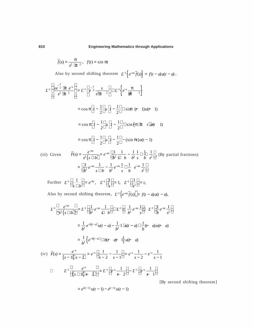
810 Engineering Mathematics through Applications
2 2( ) , ( ) sinf s f t t
sπ= = π+ π
Also by second shifting theorem 1 ( ) ( ) ( )asL e f s f t a u t a− − = − − ,
21 1 122 2 2 2 2 2
sss
sse e sL L e L es s s
− − −− − − − + π π= + + π + π + π
1 1cos sin ( 1) ( 1)2 2
t u t t u t = π − − + π − −
( )1 1cos sin ( 1)2 2
t u t t u t = π − − + −π + π −
1 1cos (sin ) ( 1)2 2
t u t t u t = π − − − π −
(iii) Given ( )2 2 2 21 1 1 1 1 1( )
asaseF s e
s s b b s b b s b s
−− = = − + ⋅ + +
, (By partial fractions)
2 2 21 1 1 1 1 1as as ase e eb s b b s b s
− − − = − + +
Further 1 1 12
1 1 1, 1, ,btL e L L ts b s s
− − − − = = = +
Also by second shifting theorem, ( )1 ( ) ( ) ( ),asL e f s f t a u t a− − = − −
( )1 1 1 1
2 2 2 21 1 1 1 1 1as
as as aseL L e L e L es s b b s b b s b s
−− − − − − − − = + − + + +
( )2 21 1 1( ) 1 ( ) ( ) ( )b t ae u t a u t a t a u t ab b b
− −= − − ⋅ − + − −
( ) 21 ( ) 1 ( )b t ae b t a u t ab
− −= + − − −
(iv)( )( )
1 1 1 1( )1 2 2 1 2 1
ss s seF s e e e
s s s s s s
−− − − = = − = − − − − − − −
⇒ ( )( )1 1 11 1
1 2 2 1
ss seL L e L e
s s s s
−− − − − − = − + − − −
[By second shifting theorem]
2( 1) ( 1)( 1) ( 1)t te u t e u t− −= − − −

Laplace Transforms and Their Applications 811
( ) ( )2 1 1 ( 1)t te e u t− − = − ⋅ −
(v) Here ( )3( ) ( )
1
saseF s e f s
s
−−= =
+, where
( )31( )
1f s
s=
+
( )( )11 2
31 ( 1) ( 1)21
steL e t u t
s
−− −−
= − − +
Example 43: Find the inverse laplace transform of ( )1
1 ss e−−.
Solution:( ) ( ) ( )11 1 1 2 31 1 11 11
s s s ssL L e L e e e
s e s s−− − − − − − −
−
= − = + + + + … −
1 1 1 2 1 31 1 1 1s s sL L e L e L es s s s
− − − − − − − = + + + + …
Comparable to ( )1 1( ) , where ( ) in each caseasL e f s f ss
− − = .
⇒ ( ) 11 1 1 1 ( 1) ( 2) ( 3)sL e u t u t u ts
−− − − = + − + − + − + … Thus, the function can be written as
1, 0 12, 1 23, 2 3( )
tttf t
< ≤ < ≤ < ≤= … …………… …………
Sometimes it is called as staircase function.
Example 44: In an electrical circuit with e.m.f. E(t), resistance R and inductance L, the
current i builds up at the rate given by ( )diL Ri E tdt
+ = . If the switch is connected at t = 0
and disconnected at t = a, find the current i at any instant.
Solution: Given i = 0 at t = 0 and , for 0( ) , for
E t aE t o t a
< <= >On taking laplace of each term of the given equation, we get
( )0
( ) (0) ( ) ( )stL s i s i R i s e E t dt∞
−− + = ∫ (L and R are constants) … (1)
f t( )
Ot
1
2
3
1 2 3
Fig. 12.8

812 Engineering Mathematics through Applications
( )0
( ) 0a
st st
aLs R i s e E dt e dt
∞− −+ = +∫ ∫
( )( ) ( ) 1as t
as
o
e ELs R i s E es s
−−+ = = −
−
⇒ ( ) ( )1( )
asei s Es Ls R s Ls R
− = − + + … (2)
Now taking inverse laplace on both sides, we get
( ) ( )1 11 1( ) asi t EL EL e
s Ls R s Ls R− − −
= − + + … (3)
By partial Fractions, ( )1 1 1 1L
s Ls R R s R Ls R = − + + … (4)
∴ Equation (3) becomes,
1 11 1 1 1 1 1( ) asL Li t E L E L eR s R Ls R R s R Ls R
− − − = − − − + +
1 1 1 11 1 1( )
asasE E ei t L L L L eR RR s R ss s
L L
−− − − − − = − − − + +
( ) ( )1( ) 1 ( )R tLE Ei t e L F s
R R− −= − − … (5)
Now ( )1 1( ) ( ) ( ) ( )asL F s L e f s f t a u t a− − −= = − − , (By second shifting property)
∴( ) ( )( )1 11 1 1. ( ) ( ) 1 ( )
R Rt a t aas as L LL e L e u t a e u t a e u t aRs sL
− − − −− − − − − = − − − = − − + … (6)
On putting (6) into (5), we get the value of the current
( ) ( )( )( ) 1 1 ( )R Rt t aL LE Ei t e e u t a
R R− − −
= − − − − … (7)
Now, for 0 < t < a, ( )( ) 1R tLEi t e
R−
= −( ) 0, 0
1,u t a t a
t a− = < <
= ≥ Q
for t > a, ( )
( ) 1 1 1R R R Rt t a t aL L L LE E Ei t e e e e
R R R− − − −
= − − − = −

Laplace Transforms and Their Applications 813
II Unit Impulse Function (Dirac Delta Funtion)
Impulse is considered as a force of very high magnitude appliedfor just an instant and the function representing the impulse is calledDirac–Delta Function.
Mathematically, it is the limiting form of the function
1 ,( )0, otherwise, as 0
a t at a ∈
∈≤ ≤ + ∈δ − = ∈→
It is apparent from the figure 12.9, that as ∈ → 0, the height ofthe strip increases indefinitely and the width decreases in such away that the area of the strip is always unity.
The above fact can notionally be stated as ( ) , for, for
t a t ao t a
δ − = ∞ = ≠
such that
0
( ) 1 for 0t a dt a∞
δ − = ≥∫
Observation: In mechanics, the impulse of a force f(t) over a time interval, say a ≤ t ≤ (a + ∈) is defined to be theintegral of f(t) from a to (a + ∈). The analog of an electric circuit is the integral of e.m.f. applied to the circuit,integrated from a to (a + ∈). Of particular practical interest is the case of very short ε with limit ε → 0 i.e. impulseof a force acting for an instant.
Transform Of Unit Impulse Function:
[ ]0 0
1( ) ( )aa
st st st st
a aL t a e t a dt e odt e dt e odt
+∈∞ ∞− − − −
+∈δ − = δ − = + +
∈∫ ∫ ∫ ∫
( )1 1 1 1aa st as s
s ast as
a a
e e ee dt e es s s
+∈+∈ − − − ∈− +∈− − − = = = − + = ∈ ∈ − ∈ ∈
∫
Taking Limit as ∈ → o,
[ ]0
1 1( )as s s
as as
o
e e eL t a Lt e Lt es s
− − ∈ − ∈− −
∈→ ∈→
− −δ − = = ⋅ = ∈ ∈In particular, if a = o, L[δ(t)] = 1.
Filtering of unit Impulse Function:
If f(t) is continuous and integrable for all t ≥ 0, then 0
( ) ( ) ( )f t t a dt f a∞
δ − =∫
Relation Bewteen u’(t – a) and δ(t – a)
[ ] [ ] [ ]( ) ( ) ( ) ( )as
aseL u t a sL u t a u a s o e L t as
−−− = − − − = − = = δ −′
Example 45: The differential equation governing the flow of a current i(t) in an LR circuitis given by
( )diRi L E tdt
+ = δ
1
∈δ∈( – )t a
a a + ∈Ot
Fig. 12.9

814 Engineering Mathematics through Applications
where E δ(t) is the impulse voltage and i(0) = 0. Find the current i(t), t > 0.
Solution: On taking laplace of each individual term in the given equation,
( ) ( ) ( ) .1Ri s L s i s i o E + − =
implying ( ) ( ) or ( )
ELR Ls i s E i s Rs
L
+ = =+
On taking inverse, laplace, ( )R tLEi t e
L−
= is the required expression for the current i.
Example 46: An impulsion voltage Eδδδδδ(t) is applied to an L C R circuit with zero initialcondition. If i(t) be the current at any subsequent time t, find the limit of i(t) as t →→→→→ 0.
Solution: The governing equation for an L C R circuit is
1 ( )
t
o
diL Ri i dt E tdt C
+ + = δ∫ , where i(t) = 0 when t = 0
Taking Laplace of each individual term on both sides of the equation,
( )1( ) (0) ( ) ,i sR Esi s i i s
L CL s L − + + = where i(0) = 0
Implying, 1 1 ( )R Es i sL CL s L
+ + = or 2 1 ( )R Es s i s s
L CL L + + =
( )2 2 22( ) 1 2
E s E si s RL L s as a bs sL CL
= =+ + ++ + 2 21where 2 andR a a b
L CL= = +
( )
( ) ( )2 2 2 22 2
( ) 1( ) ,( )
s a a s aE Ei s as a bL L s a b s a b
+ − + = − + + + + + +
On inversion, ( ) cos sinat atE ai t e bt e btL b
− − = −
Taking limits as t → 0, EiL
→ . Though, initially current is applied, yet a large current will
develop instantaneously due to impulse applied at t = 0 and it is EL
.
ASSIGNMENT 5
1. Sketch the graph of the following function and express them is terms of unit stepfunction. Hence find their laplace transforms:
(i)2 , for 0
( ) 1, fort t
f t t< < π
> π

Laplace Transforms and Their Applications 815
(ii) 20 for 0
( ), for
t af t
t t a< <= >
[Hint: f(t) = t2ua(t)]
2. Find the laplace transform of the followings:
(i) ( )0,
( ) cos , 0t T
f t t t T>= ω + φ < <
(ii), for , where 0
( ) 0 for andk a t b a
f t o t a t b< < >= < < >
(iii)
1 , 0( )
0,
t hf t h
t h
< <= >
[Hint: Expessible as f(t) = 1h [1 – uh(t)]]
(iv)3 , 0 1( )
0 1
te tf tt
< <= > [Hint: f(t) = [1 – u1(t)]e
3t]
(v) 0, 0( ) sin ,
tf t t t
< < π= > π [Hint: f(t) = sin t uπ(t)]
(vi) sin , 0( ) 0,
t tf t t
< ≤ π= > π [ ] [ ]Hint : ( ) sin 1 ( ) ( ) sin sin ( )f t t u t t u t t t t u tπ π π = − + = + −
3. Find the inverse transform of
(i)* 2 1
ses
−π
+ (ii) 2
ases
−(iii) 2 2
asses b
−
+ (iv) 21
4
ses
−π−+ *[KUK, 2004]
4. Solve y” + 4y’ + 3y = f(t), where ( ) 1, 0
0,f t t a
t a= < <
= > ; given that y(0) = y’(0) = 0
( )1Hint: ( ) 1 ( ), ( ) 1 , ( ) ( ) ( )( 1)( 3)
asa af t u t y s e y t f t a u t
s s s− = − = − = − + +
5. A beam has its ends clamped at x = 0 and x = l. A concentrated load W acts vertically
downwards at the point 3
x = l . Find the resulting defection.
4
4Hint: The differential equation and boundary conditions are
3and (0) (0) ( ) ( ) 0
d yx
dx EIy y y l y l
ω = δ − = = = =′ ′
l
6. A cantilever beam is clamped at the end x = 0 and is free at the end x = l. It carries auniform load per unit length from x = 0 to x = l/2. Calculate the deflection y at anypoint.
( )
4
4
0,
( )Hint: The differential equation and boundary condition ,
020 ; ( ) and (0) (0) 0 (0) (0)
0, 2
d y xdx EI
w xx x y y y y
x
ω= < < < < ω = = = = =′ ′′ ′′′ >
l
l
l

816 Engineering Mathematics through Applications
III Laplace Transform of Periodic Functions
If f(t) be a periodic function of period, T(> 0) i.e. f(t + T) = f(t), then
( )0
( )( )
1
Tst
sT
e f t dtLf t
e
−
−=−
∫
Proof: By definition,
2 3
0 0 2( ) ( ) ( ) ( ) ( )
t t tst st st st
t tLf t e f t dt e f t dt e f t dt e f t dt
∞− − − −= = + + + ……∫ ∫ ∫ ∫
Substituting t = u, t = u + T, t = u + 2T, in the successive integrals, then
( ) ( 2 )
0 0 0( ) ( ) ( ) ( 2 )
T T Tsu s u T s u TLf t e f u du e f u T du e f u T du− − + − += + + + + + ……∫ ∫ ∫
Since f(u) = f(u + T) = f(u + 2T) = …,
∴ 2
0 0 0[ ( ) ( ) ( ) ( )
T T Tsu sT su sT suL f t e f u du e e f u du e e f u du− − − − −= + + + ……∫ ∫ ∫
( )2
01 ( )
TsT sT sue e e f u du− − −= + + + … ∫
( ) 0
1 ( )1
Tsu
sTe f u du
e−
−=− ∫ (On changing the dummy variable u to t)
( ) ( )0
( )( )
1
Tst
sT
e f t dtL f t
e
−
−=−
∫
Observation: Hence the laplace transform of a periodic function f(t) with period T is expressible in the form of
integral 0
( )T
ste f t dt−∫ over one period of f(t) instead of over the semi-infinite interval 0 ≤ t ≤ ∞.
Example 47: Find the laplace transform of the triangular wave of period 2a given by
( ) , 02 , 2
f t t t aa t a t a
= < <= − < <
[Madras, 2000; UP Tech, 2002; VTU, 2003; KUK, 2004; NIT Jalandhar, 2006]
Or
Find the laplace transform of the triangular wave function f(t) whose graph is shownbelow.
Solution: Clearly the graph of f(t) is a straight line from the origin with slop 1 in the intervalo ≤ t ≤ a
∴ f(t) = t, o ≤ t ≤ aHowever in the interval a ≤ t ≤ 2a, the graph is a straight line whose slope is -1.

Laplace Transforms and Their Applications 817
∴ f(t) = (– 1)(t – 2a) = 2a – t, a ≤ t ≤ 2aThus, the function is a periodic one, with period 2a
0 a 2a 3a 4a
f(t)
t
Fig. 12.10
∴ 2
20
1[ ( )] ( )1
ast
asL f t e f t dte
−−=
− ∫
2
21 ( ) (2 )
1
a ast st
aso ae f t dt e a t dt
e− −
−
= + − −
∫ ∫
2
2 2 21 (2 )
1
a ast st st st
aso a
e e e et a te s s s s
− − − −
−
= − + − + − − −
2
2 2 2 2 21 1
1
asas as as as
as
ee e e ea ae s s s s s s
−− − − −
−
= − + + + − − −
( )22 2
1 1 2 11
as asas e e
e s− −
− = − + −
( ) ( )2
2 21 1
1as
as es e
−−= −
−
( ) ( ) 2/2 /2 /22
1 as as asas as as e e e
s e e e− − −
− − = − −
( )( ) ( )2/2 /22 /2 /2 /2 /2
1 as asas as as as e e
s e e e e−
− −= −− +
21 tanh
2as
s =
Example 48: Find the laplace transform of the full wave rectifier f(t) = Esinωωωωωt, o < t < πππππ/ωωωωω;having period πππππ/ω.ω.ω.ω.ω.
Solution:/
0
1( ) sin1
wst
sLf t e E t dte
π−
− πω
= ω−
∫

818 Engineering Mathematics through Applications
( )/
2 20
sin cos1
wst
sE e s t t
se
π−
− πω
= − ω − ω ω + ω −
( )/
2 2 2 21sin cos 0
1
s
sE e
s se
− π ω
− πω
π = − π − ω ω − − ω + ω ω + ω −
/
2 2 2 21
s
sE e
s se
− π ω
− πω
ω= ω + + ω + ω −
( )( ) ( )/2 2 /
11
ss
E es e
− π ω− π ω
⋅ ω= ++ ω −
/
2 2 /1
( ) 1
s
sE e
s e
− π ω
− π ωω +=
+ ω −
2 2coth
( ) 2E s
sω π=
+ ω ω2
21coth1
x x x
x x xe e exe e e
− −
− − + + = = − −Q
The graph for the function f(t) which is a full-sine wave rectifier can be drawn as below:
y a =
Y
0 π ω/ 2π ω/ 3π ω/ X– /π ω
Fig. 12.11
Since sin sin for all .w t t tπ + = ω ω
Example 49: Find the laplace transform of the square wave (or meander) function of aperiod a defined as: f(t) = 1 when 0 < t < a/2
= –1, when a/2 < t < a [UP Tech, 2004]
Solution: [ ] 1( ) ( )1
ast
aso
f tL e f t dte
−−=
− ∫
/2
/2
1 1 ( 1)1
a ast st
aso a
e dt e dte
− −−
= ⋅ + − −
∫ ∫

Laplace Transforms and Their Applications 819
/2
/2
11
a ast st
aso a
e ee s s
− −
−
= − − − −
/2 /21 1 111
sa as asas e e e
e s s− − −
− = − + − − −
( )/21 1 2
1sa as
as e es e
− −− = − + −
( ) ( )2/21 11
saas e
s e−
−= −−
( )( )
( )( )
/2 /4 /4
/2 /4 /4
11 1 1 tanh1 4
sa sa sa
sa sa sa
e e e ass e s e e s
− −
− −
− −= = =
+ +
Note: It may be defined like, f(t) = k, when 0 < t < a/2 = – k, when a/2 < t < a
Y
XX– a a/2 a 3a 2a 5
k
o
– k
—2—2 —2 a
Fig. 12.12
Example 50: Find the Laplace Transform of the periodic function (saw tooth wave),
f(t + T) = f(t); ( ) for 0tf t k t TT
= < <
Solution:0 0
1 1[ ( )] ( )1 1
T Tst st
sT sTtL f t e f t dt e k dt
e e T− −
− −= =− −∫ ∫
0
11
Tst
sTk e t dt
e T−
−=
− ∫
( ) 11
Tst st
sTo
k e et dtT e s s
− −
− = − ⋅ − − − ∫ (By parts)
( ) 21
Tst st
sTo
t ek eT e s s
− −
− = − − −

820 Engineering Mathematics through Applications
( ) 2 21
1
sT sT
sTk Te e
T e s s s
− −
− = − + − −
( ) ( )21 1
1
sTsT
sTk Te e
T e s s
−−
− = + − − −
( )2 1
sT
sTk ke
s T s e
−
−= −−
Note: It may result to a particular case: when k = 1, ( )t
f TT
=
– 2T – T T0 2Tt
f t( )
Fig. 12.13
Example 51: Find the Laplace transform of the function (Half wave rectifier)
sin , for 0( ) 20, for
t tf t
t
π ω < < ω= π π< <ω ω
[Madras, 2003; KUK, 2005]
Solution:0
1[ ( )] ( )1
Tst
sTL f t e f t dt
e−
−=
− ∫
/
20
1 ( )1
sts e f t dt
e
π ω−
− πω
=−
∫ 2( ) has a period,f t T π = ω Q
/ 2 /
20 /
1 sin1
st sts e t dt e o dt
e
π ω π ω− −
− ππ ωω
= ω + × ×
−∫ ∫
/
21 sin ,
1
sts
oe t dt
e
π ω−
− πω
= ω−
∫
Using ( )2 2sin sin cos
axax ee bx dx a bx b bx
a b= −
+∫ ,

Laplace Transforms and Their Applications 821
( ) /
2 2 20
sin cos1
1
st
s
e s t t
se
π ω−
− πω
− ω −ω ω= + ω −
( ) 2 221
1
s
ses
e
−πω
− πω
ω + ω = + ω
−
( )2
2 2
1
1
sw
se
s e
π +ω
− πω
ω + =
+ ω −
( )2
2 2 1s
s e− π
ω
ω=
+ ω −
0 π ω/ 2 /π ω 3πω
4πω
5πω
Fig. 12.14
Note: Clearly the function f(t) = sinωt represents the half sine wave rectifier with period 2πω
. The graph of f(t) in the
internal 0 tπ< <ω
is sine function which varnishes at t = 0 and tπ=ω
and f(t) = 0 for the rest half from 2
toπ πω ω .
Example 52: A periodic square wave function f(t), in terms of unit step functions, is writtenas f(t) = k [u0(t) – 2ua(t) + 2u2a(t) – 2u3a(t) + …]. Show that the Laplace transform of f(t) is
given by [ ( )] tanh2
k asL f ts
= .
Solution: f(t) = k[u0(t) – 2ua(t) + 2u2a(t) – 2u3a(t) + ……]∴ L f(t) = k0[Lu0(t) – 2Lua(t) + 2L u2a(t) – 2Lu3a(t) + ……]
2 31 2 2 2
as as ase e eks s s s
− − − = − + − + ……
2 31 2 2 2as as ask e e es
− − −= − + − + ……
( )2 31 2 as as ask e e es
− − − = − − + − ……
as
ask es e
1 21
−
− = − +

822 Engineering Mathematics through Applications
1 2
1
as as
ask e es e
− −
− + − = +
as asas
as asask e k e es e s
e e
2 2
2 2
11
−−
−−
− − = = + +
tanh2
k ass
=
0 2 T– T T
t
f t( )
T
Fig. 12.15
ASSIGNMENT 6
Find the Laplace transform of the following periodic functions:
1. ( ) sin , 0 when ( ) ( );f t t t f t f t T T π= ω ≥ = + =ω
[Hint: f(t) represents full sine wave rectifier. Ex. 48]
2. Saw tooth wave function of period T given by 2( ) , 0atf t a t TT
= − + ≤ <
3. Non–Symmetric square wave of period T, given by ≤ <= − ≤ <
, 0( ) ,
a t bf t a b t T
4. Staircase function defined by f(t) = kn, nT < t <(n + 1)T; where n = 0, 1, 2,…

Laplace Transforms and Their Applications 823
ANSWERS
Assignment 1
1. (i)s
s a
3
4 4,
4+(ii)
( )2 2
4 4
2,
4
a s a
s a
++
(iii)( )2 2
4 4
2,
4
a s a
s a
−+
(iv)2
4 42 ,
4a s
s a+(v)
2
4 42 ,
4as
s a+(vi)
3
4 44 ,
4a
s a+
2. (i) 2 24a
s a+ , (ii) ( )2 2 21
s s a+
3. (i) ( ) ( )2 3
23 3 22 2 3 3 5 1
s se es s ss s s
− −− + + + − (ii)
23
2, 0
1
s
e ss
π−
>+
4. (i) ( )22 2
2 ,as
s a+(ii) ( )
2 2
22 2,s a
s a
−+
(iii) ( )22 2
2 ,as s as a
>−
(iv) ( )2 2
22 2,s a
s a
+−
5. (i)( )
2
22 2
2 ,as
s a+(ii)
( )3
22 2
2 ,a
s a+
(iii) ( )2
22 2
2 ,as s as a
>−
(iv) ( )a s a
s a
3
22 2
2 ,− >−
6. (i) ( )3
22 2,s
s a+(ii) ( )
3
22 2,s
s a−
7. (i) s bs a
1/22 2
2 2log +
+(ii)
2
21 4log2
ss
+
(iii) sa
1cot−
(iv) cot–1(s + 1)
8.a s
s a s a2 2 2 2,
+ + 9.a s
s a s a2 2 2 2,
− −
10. (i) 21 1
2 2s
s s s+
+ + (ii)2 2
2 21 log2
s bs s a
+ +
Assignment 2
1. (i) sinh ,2
t t (ii) ( )31 3 3cos2 2sin 213
te t t− +

824 Engineering Mathematics through Applications
(iii)2
/2 3 3cos 3 sin3 2 2
at ata e e at at − +
,
(iv) 3 21 4 23 15 5
t te e−+ + (v) 1 1sin2 2
tt te−−
2. ( ) ( )ate aA B bt bt B aA Ab t bt
b C2
3cos sin
2
− − ⋅ + − +
3. (i) ( )te t t21 6cos3 7 sin 33
− − , (ii) 34 t te e−− , (iii) 2 42t te e−+
4. (i) 21 sin ,2
tte t− (ii) 3t e– 3tsin t, (iii) 1 sinh2
t t
5. (i) 1 2cos tt et
−− + (ii) sin 2 ,tt
(iii)2 sinh sin
,t t
t
(iv)bt ate e
t
− −− , (v)3 2
,t t te e e
t
− − −+ − (vi) ( )2 1 cosh att
− ,
(vii) ( )2 coste t
t
− , (viii) sinte tt
−, (ix) cos cosat bt
t−
6. (i)21 cos b ta a
(ii) (1 – at)e–at, (iii) ( )2 21 4 2
2ata t at e−− +
7. (i) 2 21 1 18 4 2
tt t e− − + + (ii) ( )21 2 14
te t− + − (iii) ( )31 sinat ata
−
9. (i)bt ate ea b
− −−−
, (ii) ( )31 sin cos
2at at at
a− , (iii) ( ) ( )1 2 1t tt e e− −+ + −
(iv) ( )31 sinat ata
− , (v) ( )81 1 864
tte e t
−− − + , (vi) ( )1 cot cos2
3t t−
(vii)( )
( )2 2
sin sina at b bt
a b
−−
Assignment 3
1. t t t tx e2 2sin cos2
1 1−ω ω − ω ω = + + ω + ω +
2. cos sinBy A x x= ω + ωω
3. 3 21(2 3) ( ) 22
t t ty t e e e= + + − − 4.2
[sin cos cos( )]2ax nt nt ntn
= α − + α
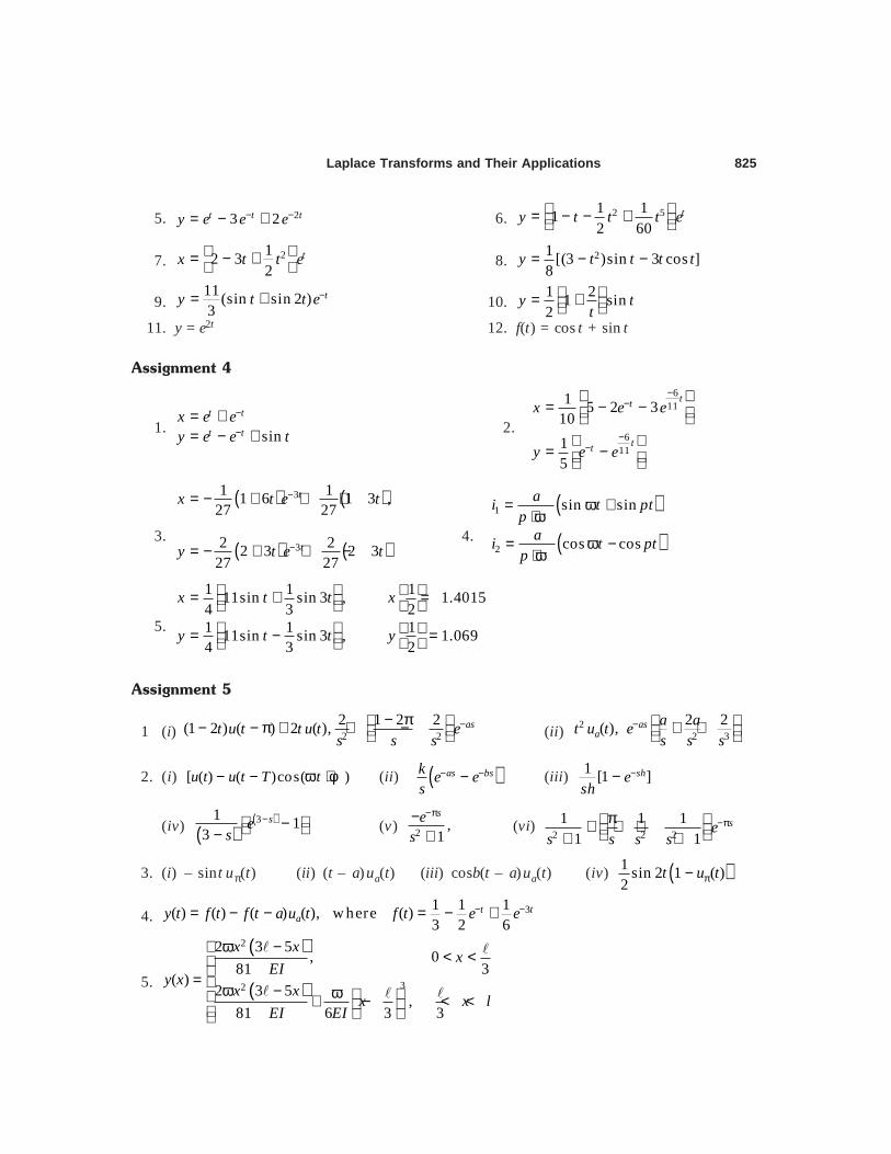
Laplace Transforms and Their Applications 825
5. 23 2t t ty e e e− −= − + 6. ty t t t e2 51 112 60
= − − +
7. tx t t e212 32
= − + 8. y t t t t21 [(3 )sin 3 cos ]8
= − −
9.11(sin sin 2 )3
ty t t e−= + 10. y tt
1 21 sin2
= + 11. y = e2t 12. f(t) = cos t + sin t
Assignment 4
1.t t
t tx e ey e e tsin
−
−= += − + 2.
611
611
1 5 2 310
15
tt
tt
x e e
y e e
−−
−−
= − −
= −
3.
( ) ( )
( ) ( )
t
t
x t e t
y t e t
3
3
1 11 6 1 3 ,27 27
2 22 3 2 327 27
−
−
= − + + +
= − + + −4.
( )
( )1
2
sin sin
cos cos
ai t ptp
ai t ptp
= ω ++ ω
= ω −+ ω
5.
1 1 111sin sin 3 , 1.40154 3 21 1 111sin sin 3 , 1.0694 3 2
x t t x
y t t y
= + = = − =
Assignment 5
1 (i) 2 22 1 2 2(1 2 ) ( ) 2 ( ), ast u t t u t es s s
−− π − − π + + − (ii) 22 3
2 2( ), asa
a at u t es s s
− + +
2. (i) [ ( ) ( )cos( )u t u t T t− − ω + φ (ii) ( )as bsk e es
− −− (iii) 1 [1 ]shesh
−−
(iv) ( )( )31 1
3se
s− − − (v) 2
,1
ses
−π−+
(vi)2 2 21 1 1
1 1se
s s s s−ππ + + + + +
3. (i) – sint uπ(t) (ii) (t – a)ua(t) (iii) cosb(t – a)ua(t) (iv) ( )1 sin 2 1 ( )2
t u tπ−
4. 31 1 1( ) ( ) ( ) ( ), where ( )3 2 6
t tay t f t f t a u t f t e e− −= − − = − +
5.
( )
( )
2
32
2 3 5, 0
81 3( )
2 3 5,
81 6 3 3
x xx
EIy x
x xx x l
EI EI
ω −< <= ω − ω + − < <
l l
l l l

826 Engineering Mathematics through Applications
6. ( ) ( )y x x x x x u xEI EI EI EIl l l l
2 42 3 4( ) 2 216 12 24 24
ω ω ω ω= − + − − −
Assignmen 6
1.2 2
cot2
E shs w
ω π+ ω
2.1 cot
22
a sThsTs
−
3.( )
( )2 1
1
sT sb
sT
a e e
s e
− −
−
− +−
4. ( )sT
sT
k es e1
−
−−