Aalborg Universitet

Estimation of CO concentration in high temperature PEM fuel cells usingelectrochemical impedanceJensen, Hans-Christian Becker; Andreasen, Søren Juhl; Kær, Søren Knudsen; Schaltz, Erik

Published in:Proceedings of the 5th International Conference on Fundamentals & Development of Fuel Cells

Publication date:2013

Document VersionEarly version, also known as pre-print

Link to publication from Aalborg University

Citation for published version (APA):Jensen, H-C. B., Andreasen, S. J., Kær, S. K., & Schaltz, E. (2013). Estimation of CO concentration in hightemperature PEM fuel cells using electrochemical impedance. In Proceedings of the 5th InternationalConference on Fundamentals & Development of Fuel Cells: FDFC 2013 European Institute for EnergyResearch (EIFER).

General rightsCopyright and moral rights for the publications made accessible in the public portal are retained by the authors and/or other copyright ownersand it is a condition of accessing publications that users recognise and abide by the legal requirements associated with these rights.

? Users may download and print one copy of any publication from the public portal for the purpose of private study or research. ? You may not further distribute the material or use it for any profit-making activity or commercial gain ? You may freely distribute the URL identifying the publication in the public portal ?

Take down policyIf you believe that this document breaches copyright please contact us at vbn@aub.aau.dk providing details, and we will remove access tothe work immediately and investigate your claim.

Downloaded from vbn.aau.dk on: maj 07, 2018

Estimation of CO concentration in high temperature PEM fuel cells usingelectrochemical impedance spectroscopy

Hans-Christian B. Jensena,∗, Søren Juhl Andreasena, Søren Knudsen Kæra, Erik Schaltza

aAalborg University, Department of Energy Technology, Pontoppidanstræde 101, DK-9220, Aalborg, Denmark

Abstract

Storing electrical energy is one of the main challenges for modern society grid systems containing increasingamounts of renewable energy from wind, solar and wave sources. Although batteries are excellent storage devices forelectrical energy, their usage is often limited by a low energy density, a possible solution, an avoidance of the longrecharging time is combining them with the use of fuel cells. Fuel cells continuously deliver electrical power as long asa proper fuel supply is maintained. The ideal fuel for fuel cells is hydrogen, which in it’s pure for has high volumetricstorage requirements. One of the solutions to this fuel storage problem is using liquid fuels such as methanol thatthrough a chemical reformer converts the fuel into a hydrogen rich gas mixture. Methanol is a liquid fuel, which haslow storage requirements and high temperature polymer electrolyte membrane (HTPEM) fuel cells can efficiently runon the reformed hydrogen rich gas, although with reduced performance depending on the contaminants, such as CO,in the gas.

By estimating the amount of CO in the fuel cell, it could be possible to adjust the fuel cell system operatingparameters to increase performance of the reformer and fuel cell stack. This work focus on the estimation of COpercentage in the hydrogen rich anode gas in a fuel cell, by combining signal processing ideas with impedanceinformation of the fuel cell while it is running. The presented approach functions during in the normal operatingrange of an HTPEM fuel cell.

Keywords: HTPEM, Fuel cell, Methanol, Reforming, CO estimation

1. Introduction

There is a growing demand for new clean energy sources, a demand which is expected to increase significantly,especially as stricter laws on emissions, which are planned, are put into force. The goal of these restrictions pointtowards zero emission, so it is not surprising that there is also a rise in the need for alternative energy sources, whichhave zero emission. Fuel cells are one of these alternative energy sources Pehnt (2001), which are used more andmore, due to their increasing reliability (Numbers are presented in Tian et al. (2010)) and cost effectiveness (Pricedevelopment for Fuel Cells are illustrated in DOE (2011)).

The state of the art method in signal processing methods regarding fuel cells is done with the impedance spectrum(There are articles on PAFC Choudhury and Rengaswamy (2006) and PEMFC Merida et al. (2006) Fuel Cells. Somecombine fault diagnosis with state of health monitoring Fouquet et al. (2006), which is the area of focus in Gebregergiset al. (2010).). The presented methods so far are not able to do this during operation and require the fuel cell to bedisconnected from the electrical load / grid during the test.

Efforts have been made in increasing operating temperatures of PEM fuel cells to minimize water managementproblems, increase fuel poisoning tolerances and decrease system complexity Zhang et al. (2006); Li et al. (2009). Inthe field of HTPEM fuel cells there is a growing interest in methanol reformers Avgouropoulos et al. (2009); Kolb et al.(2012); Jensen et al. (2007); Andreasen et al. (2008), as this gives the possibility to run on something other than pure

∗Corresponding author. Tel.: +45 9940 9267; fax: +45 9815 1411Email address: hcj@et.aau.dk (Hans-Christian B. Jensen)

Preprint submitted to Unknown November 8, 2013

hydrogen, which is proving to be one of the important factors in the full roll-out of fuel cells in commercial products.Hydrogen has high volumetric demands when it comes to storage and refueling and these are the interest of severalcompanies researching into refueling stations http://www.hydrogen.energy.gov/pdfs/review10/st001 ahluwalia 2010 o web.pdf(2010); http://www.fuelcells.org/info/charts/h2fuelingstations.pdf (2012). Methanol has the advantage of being a liq-uid fuel, but the challenge is to reform it into a hydrogen rich gas before entering the fuel cell, and the resulting fuelcell performance is highly dependent on the quality of the output reformer gas. One of the most important parameteris the CO % content, so an estimation of the CO contents is of interest for better control of the reforming process andthereby eventually also of the fuel cell system.

The fuel cell MEA used in this study is a Celtec-P2100 membrane produced by BASF with an active cell area of45[cm2]. Further information about the MEA are presented in BASF (2011b) and BASF (2011a)

This article serves as a proof of concept, analyzing the possibilities of using a signal processing based approachto obtain an estimate for the CO percentage contained in the fuel cell anode gas. This method uses a single frequencyin the impedance spectrum to estimate the CO, which results in a fast and simple prediction of the CO concentration,compared to using the entire frequency sweep normally done in impedance spectroscopy. Since the method is signalbased it requires excitation of the system through an input signal, but this signal can be introduced during normaloperation, so the system can continue operation during CO estimation.

2. Nomenclature

AMEA Area of the MEA of a single cell [cm2]FC fuel cellicell(t) Cell current [A]MEA Membrane electrode assemblyPEMFC PEM Fuel CellTcell(t) Stack temperature [C]Vcell(t) Voltage produced by a single cell [V]ZRe(t) Real part of impedance, which is the resistance [Ω cm2]ZIm(t) Imaginary part of impedance, which is the reactance[Ω cm2]

2.1. Electrochemical Impedance Spectroscopy

Electrochemical impedance spectroscopy (EIS) is a well known characterisation method for electrochemical de-vices, and have been studied by several authors for use a characterisation tool for fuel cells both within modelling andstate-of-health monitoring Yuan et al. (2007); Andreasen et al. (2011). The typical use of EIS with fuel cells involvessuper positioning a small amplitude sine wave signal to the DC current (galvanostatic measurement) or voltage (poten-tiostatic measurement) drawn from the fuel cell. Figure 1 shows the polarisation curve of a given fuel cell, illustratingthat drawing a sinewave shaped current results in a voltage response also exhibiting sinusoidal behaviour, althoughwith a different amplitude and phase depending on the different internal states of the fuel cell under test. In order toget pure sine wave behaviour the measurements typically need to be conducted at the linear area of the polarisationcurve otherwise the resulting voltage response on a galvanostatic measurement will not yield a true sine wave output.For this reason the superimposed signals also need to be small in amplitude to avoid entering nonlinear regions of thepolarisation curve.

Using signals with varying frequencies, the impedance of the fuel cell under test can be calculated by extractingthe amplitudes and phase shifts of the current and voltage.

Using the extracted amplitudes (AU and AI) and phase shift (φ), the real (α) and imaginary part (β) of impedanceZFC = α + j · β can be calculated using equation 1 and 2 respectively.

α = Re(

AU

AI(cos(φ) + jsin(φ))

)=

AU

AI(cos(φ)) (1)

β = Im(

AU

AI(cos(φ) + jsin(φ))

)=

AU

AI(sin(φ)) (2)

2

IDC

Current [A]

Cell

Volta

ge [V

]UFC

Figure 1: Graph showing how super positioning a small amplitude current sine wave results in sine wave voltage response.

This impedance describes the overall electrical behaviour of the fuel cell, a behaviour governed by all the differentchemical and electrochemical processes occurring, diffusion of gasses and resistances in the different layers of thefuel cell. The impedance can be evaluated looking at magnitude and phase plot or as Nyquist plots, such as the oneshown in figure 2, where the impedance of the HTPEM fuel cell under test is shown running on pure hydrogen at ananode stoichiometry of λA = 1.3, a cathode stoichiometry of λC = 4, a DC current of IDC at different temperatures.

0.2 0.25 0.3 0.35 0.4 0.45 0.5 0.55 0.6 0.65-0.02

0

0.02

0.04

0.06

0.08

0.1

0.12

0.14

Pure hydrogen, H

2

=1.2, Air

=4, IDC

=10A

ZRe

[ cm2]

-ZIm

[ c

m2 ]

T=120oCT=130oCT=140oCT=150oCT=160oCT=170oCT=180oC1000Hz100Hz10Hz1Hz0.1Hz

Figure 2: Nyquist plot of the HTPEM fuel cell impedance at IDC=10A, on pure hydrogen at different temperatures.

The shown impedance can be analyzed using different modeling approaches an equivalent electrical circuit modelcan be found for system simulations of the fuel cell, or other aspects of fuel cell performance can be analyzed.

3

3. Experimental setup

For examining the fuel cell under test, an experimental setup is used, where a single cell assembly consisting ofa BASF P2100 fuel cell mounted between two PTFE gaskets, carbon composite flow plates all clamped together bystainless steel endplates with cartridge heaters for keeping a constant fuel cell temperature during operation. Theassembly is shown in figure 3. The anode gas is supplied by three Burkert 8711 mass flow controllers (MFC),enabling the introduction of different concentrations of H2, CO and CO2, all typical components in fuel cells fuelledby reformers. The cathode side is in a similar way controlled by a Burkert 8712 MFC supplied by compressed air.The data acquisition, control and automation of the different tests conducted by a Labview virtual interface and threeNational Instruments PCI units, NI PCI 6229, NI PCI 4351 and NI PCI 6704

Figure 3: Picture of the test setup.

The current drawn from the fuel cell is effectuated by a 800W TDI Power RBL488 50-150-800 electronic load,and an additional Labview based system, using a PCI 6259 is used to conduct the impedance measurements. Thesettings for the impedance system when measuring the full impedance spectrum is as follows:

• Frequency range 1kHz to 0.1Hz

• Max current amplitude 3A

• 25 frequencies per logarithmic decade

The CO estimation algorithm is implemented in the Labview impedance measurement systems and provided withthree input measurements needed as for the CO estimation algorithm. These are current icell(t), voltage Vcell(t) andtemperature Tcell(t).

4

4. CO estimator algorithms

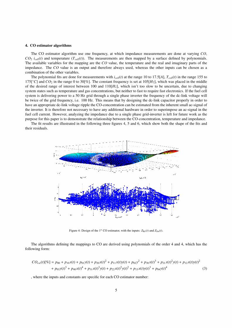
The CO estimator algorithm use one frequency, at which impedance measurements are done at varying CO,CO2 icell(t) and temperature (Tcell(t)). The measurements are then mapped by a surface defined by polynomials.The available variables for the mapping are the CO value, the temperature and the real and imaginary parts of theimpedance. The CO value is an output and therefore always used, whereas the other inputs can be chosen as acombination of the other variables.

The polynomial fits are done for measurements with icell(t) at the range 10 to 17.5[A], Tcell(t) in the range 155 to175[C] and CO2 in the range 0 to 30[%]. The constant frequency is set at 105[Hz], which was placed in the middleof the desired range of interest between 100 and 110[Hz], which isn’t too slow to be uncertain, due to changingsystem states such as temperature and gas concentrations, but neither to fast to require fast electronics. If the fuel cellsystem is delivering power to a 50 Hz grid through a single phase inverter the frequency of the dc-link voltage willbe twice of the grid frequency, i.e. 100 Hz. This means that by designing the dc-link capacitor properly in order tohave an appropriate dc-link voltage ripple the CO-concentration can be estimated from the inherent small ac-signal ofthe inverter. It is therefore not necessary to have any additional hardware in order to superimpose an ac-signal in thefuel cell current. However, analyzing the impedance due to a single phase grid-inverter is left for future work as thepurpose for this paper is to demonstrate the relationship between the CO-concentration, temperature and impedance.

The fit results are illustrated in the following three figures 4, 5 and 6, which show both the shape of the fits andtheir residuals.

Figure 4: Design of the 1st CO estimator, with the inputs: ZRe(t) and ZIm(t).

The algorithms defining the mappings to CO are derived using polynomials of the order 4 and 4, which has thefollowing form:

COest(t)[%] = p00 + p10x(t) + p01y(t) + p20x(t)2 + p11x(t)y(t) + p02y2 + p30x(t)3 + p21x(t)2y(t) + p12x(t)y(t)2

+ p03y(t)3 + p40x(t)4 + p31x(t)3y(t) + p22x(t)2y(t)2 + p13x(t)y(t)3 + p04y(t)4 (3)

, where the inputs and constants are specific for each CO estimator number:

5

Figure 5: Design of the 2nd CO estimator, with the inputs: ZRe(t) and Tcell(t).

1. x(t) is the real part of the impedance measurement (ZRe(t)), y(t) is the imaginary part of the impedance mea-surement (ZIm(t)) and the constants are:

p00 = 974.86998357924824, p10 = 355652.89198044885, p01 = -719017.06812596519p20 = 13651868.496985577, p11 = -164331357.03022113, p02 = 192603361.51394019p30 = 8923826118.2576504, p21 = -10405152921.542259, p12 = 26737014581.621918p03 = -22524744938.23312, p40 = -3856269810854.4072, p31 = 4235101263284.8267p22 = -1634213550500.0017, p13 = -874591099518.78516, p04 = 927327446188.15051

2. x(t) is the real part of the impedance measurement (ZRe(t)), y(t) is the temperature measurement (Tcell(t)) andthe constants are:

p00 = 1787.6150832153778, p10 = 1463318.473086644, p01 =-58.795638262515595p20 = -278784271.84294492, p11 = -20257.273369942086, p02 = 0.63971065306233743p30 = 15592241318.218281, p21 = 2863913.5993069424, p12 = 89.318472127976719p03 = -0.0028821293407541378, p40 = -55260546104.019379, p31 = -93627348.27086834p22 = -7093.0558676384117, p13 = -0.12320688595788029, p04 = 4.646738529168038e-6

3. x(t) is the imaginary part of the impedance measurement (ZIm(t)), y(t) is the temperature measurement (Tcell(t))and the constants are:

p00 = -5480.7538313315272, p10 = 1002880.7779525866, p01 = 91.432572873854767p20 = -124845012.19590963, p11 = -7736.6653833052951, p02 = -0.6699016704172126p30 = 3629480091.6688304, p21 = 1055462.7823221444, p12 = 2.1462557021521174p03 = 0.0026690942152858481, p40 = -258675025328.43097, p31 = 20611436.140699334p22 = -4403.4762059475961, p13 = 0.11716504040925634 , p04 = -5.2164030092854899e-6

4.1. Preliminary analysis of the algorithmsThe polynomial fit errors are presented in table 1.The algorithms can be analysed in three ways. The first is the errors from table 1, which shows that the polynomial

with the ZRe(t) and Tcell(t) inputs is the best by at least 35%. It is followed by the polynomial with the ZRe(t) and ZIm(t)inputs, which is an improvement by around 12% over the last polynomial fit.

The second way to analyse the polynomial fits is with the figures. The polynomial with the ZRe(t) and ZIm(t) inputshave inputs that are clustered in an arc, which is expected from impedance results, but as they don’t span the whole

6

Figure 6: Design of the 3rd CO estimator, with the inputs: ZIm(t) and Tcell(t).

CO Input FitEstimator Variables Results# 1st 2nd R2 Adjusted R2 RMSE

1 ZRe(t) ZIm(t) 0.8001512083869896 0.7996319279336521 0.382534415303188662 ZRe(t) Tcell(t) 0.8908355506039385 0.8905519013293385 0.282722494626135633 ZIm(t) Tcell(t) 0.7487133659915381 0.7480604311592964 0.428947799657735

Table 1: Table for polynomial plane error values.

surface and just a part of it, then there is less robustness in the mapped plane. This translates a higher uncertainty,when the system ages. The other two polynomials span the mapped plane nicely and are therefore expected to havebetter robustness.

The third way to analyse the polynomials is by evaluating their constants. Again the polynomial with the ZRe(t)and ZIm(t) inputs stand out with larger higher order constants than the other two. This is also visible in the figures ofthe polynomials as the mapped surface reach higher CO values than the other two polynomials by a factor of at least300%. This indicates less robustness for the polynomial with the ZRe(t) and ZIm(t) inputs, but it doesn’t guarantee it.

5. Experimental results

The polynomial fits are designed for measurements done with icell(t) in the range 10 to 17.5[A], Tcell(t) in the range155 to 175[C] and CO2 in the range 0 to 30%, while the tests are done in almost the same range, though with theextension of Tcell(t) in the range 155 to 180[C]. The algorithms aren’t designed for 180[C], but this was included toshow robustness outside the operating range.

The following subsections are comprised of test results with or without filtering, where the first subsection containsthe results obtained without filtering, while the second subsection contains the results with the filtering.

7

0

2

4 155° 160° 165° 170° 175° 180°

CO

est #

1[%]

0

2

4

CO

est #

2[%]

0

2

4

CO

est #

3[%]

Test[#]

Figure 7: Plot unfiltered.

5.1. Verification testThe figure 7 illustrates the test results of the CO estimators. The shapes of the first and third CO estimators are

comparable, as they both have problems estimating at the lower temperatures where zero is estimated acceptable, butany other CO value results the same estimate. When the temperature rises, then they both also start following the COvalue. The second CO estimator differs as this seem to follow the CO value for any temperature.

The third CO estimator has a good tracking performance in the temperature range 170 − 175[C], and a decenttracking performance (Error is less than 1.5[%]). While the first has a decent tracking performance (Error is aroundthan 2[%]). The second CO estimator also show relation to the temperature, as icell(t) has a higher influence on theprecision at higher temperature.

5.2. Filtered verification testThe mean filtered tests results presented in figure 9 have a smaller variation than the unfiltered results in figure

7. The offset of the filtered tests follow the same characteristics and shape as for the unfiltered tests. Hence the jittershown in the results aren’t pure white noise. Furthermore, the carry frequency of the noise is the same frequency asthe changes in the test parameters.

The difference between the error plots for the filtered and non-filtered test results are small, but the is one notibleand that is for the second CO estimator at 180[] and 0% CO in the fuel. Here the filter actually increase the error.

8

0

1

2

3155° 160° 165° 170° 175° 180°

CO

est #

1[%]

0

0.5

1

CO

est #

2[%]

0

0.5

1

1.5

CO

est #

3[%]

Test[#]

Figure 8: Unfiltered error between estimate and real value.

6. Conclusion

The figure 7 illustrates the CO estimators 1 and 3 both fail to follow the CO value at lower temperatures, whilethere is no such problem with the second CO estimator. This indicate a strong relation between ZRe(t), Tcell(t), andCO concentration.

The presented CO estimators delivers acceptable results, but there are differences between their performance.There isn’t one algorithm that is better than others for all situations, but there is one that overall has better performanceand that is the second CO estimator, which provides acceptable results in most situations, but is surpassed at lowerCO values.

The first CO estimator provides good CO estimation at 0%, and lower CO values at increasing temperatures. Thishowever doesn’t stop the CO estimator from giving the worst estimations at the other end.

The main improvement in the presented paper is the runtime CO estimation methods, which prove promisingresults. The other alternatives at the present time are either a gas analyser, as known CO sensors are cross gassensitive, or methods under research, e.g. impedance spectroscopy.

9

0

2

4 155° 160° 165° 170° 175° 180°

CO

est #

1[%]

0

2

4

CO

est #

2[%]

0

2

4

CO

est #

3[%]

Test[#]

Figure 9: Plot mean filtered with a filter length of 3 samples.

7. Future work

The next step is to implement the approach on a different setup with either a reformer or a fuel cell stack. Aexperimental setup with a reformer can be used to test the desired improved performance, which should come withthe knowledge about CO contents. Whereas a setup with a fuel cell stack rather than a experimental setup would provethe functionality of the approach on a real setup with appropriate measurement values and noise.

Appendix

The results are presented in the following table. The table .2 contains the largest deviation obtained with thefiltered results for all the CO estimators. The following three tables (.3,.4 and .5) has the filtered results for all the COestimators in higher detail.Andreasen, S. J., Kær, S. K., Nielsen, M. P., 2008. Experimental evaluation of a pt-based heat exchanger methanol reformer for a HTPEM fuel cell

stack. Electrochemical Society Transactions 12, 571–578.Andreasen, S. J., Vang, J. R., Kær, S. K., 2011. High temperature pem fuel cell performance characterisation with co and co2 using electrochemical

impedance spectroscopy. International Journal of Hydrogen Energy 36, 9815–9830.Avgouropoulos, G., Papavasiliou, J., Daletou, M. K., Kallitsis, J. K., Ioannides, T., Neophytides, S., 2009. Reforming methanol to electricity in a

high temperature pem fuel cell. Applied Catalysis B: Environmental Issues 3-4 90, 628–632.

10

0

1

2

3155° 160° 165° 170° 175° 180°

CO

est #

1[%]

0

0.5

1

CO

est #

2[%]

0

0.5

1

1.5

CO

est #

3[%]

Test[#]

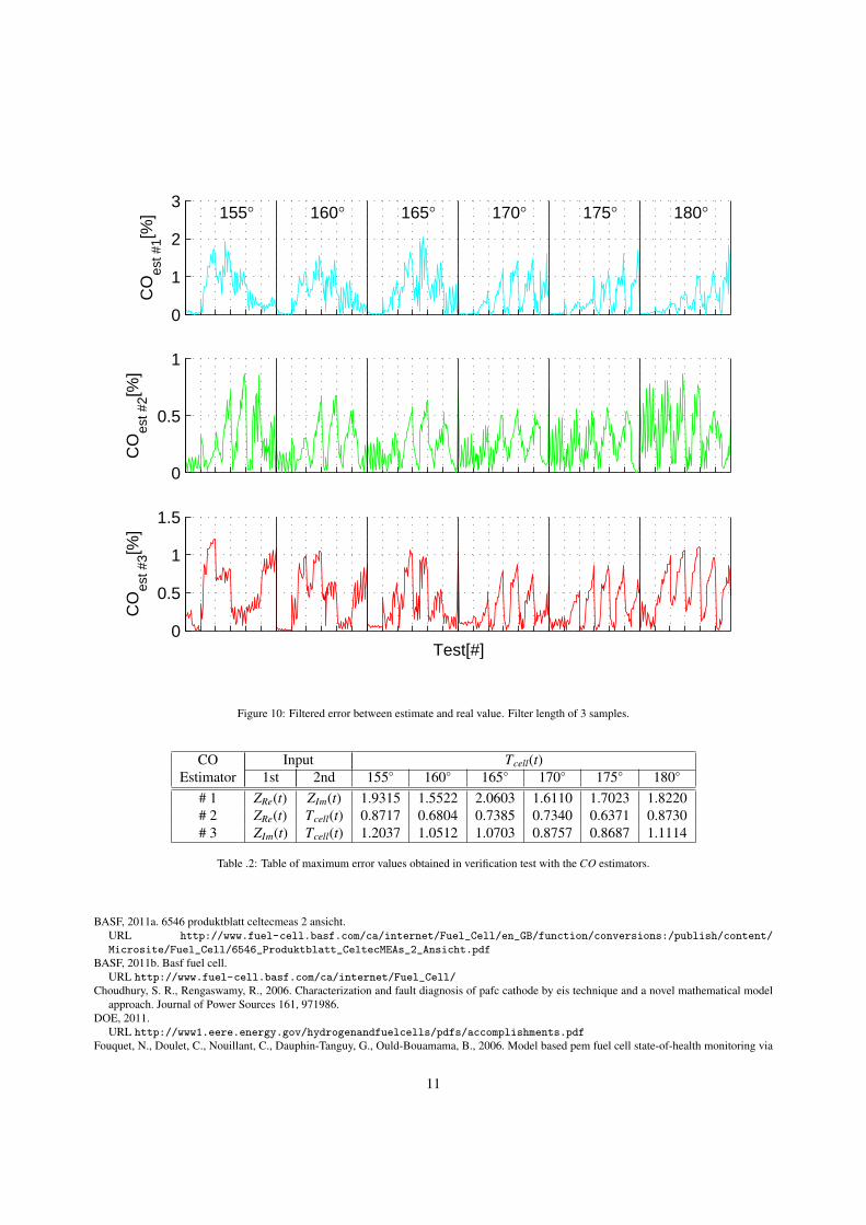
Figure 10: Filtered error between estimate and real value. Filter length of 3 samples.

CO Input Tcell(t)Estimator 1st 2nd 155 160 165 170 175 180

# 1 ZRe(t) ZIm(t) 1.9315 1.5522 2.0603 1.6110 1.7023 1.8220# 2 ZRe(t) Tcell(t) 0.8717 0.6804 0.7385 0.7340 0.6371 0.8730# 3 ZIm(t) Tcell(t) 1.2037 1.0512 1.0703 0.8757 0.8687 1.1114

Table .2: Table of maximum error values obtained in verification test with the CO estimators.

BASF, 2011a. 6546 produktblatt celtecmeas 2 ansicht.URL http://www.fuel-cell.basf.com/ca/internet/Fuel_Cell/en_GB/function/conversions:/publish/content/

Microsite/Fuel_Cell/6546_Produktblatt_CeltecMEAs_2_Ansicht.pdf

BASF, 2011b. Basf fuel cell.URL http://www.fuel-cell.basf.com/ca/internet/Fuel_Cell/

Choudhury, S. R., Rengaswamy, R., 2006. Characterization and fault diagnosis of pafc cathode by eis technique and a novel mathematical modelapproach. Journal of Power Sources 161, 971986.

DOE, 2011.URL http://www1.eere.energy.gov/hydrogenandfuelcells/pdfs/accomplishments.pdf

Fouquet, N., Doulet, C., Nouillant, C., Dauphin-Tanguy, G., Ould-Bouamama, B., 2006. Model based pem fuel cell state-of-health monitoring via

11

COTcell(t) 0[%] 0.5[%] 1[%] 1.5[%] 2[%] 2.5[%]155 0.1259 1.7426 1.9315 1.2058 0.7729 0.4566160 0.1371 1.1294 1.5522 1.4369 0.8951 0.5645165 0.1099 0.8948 1.6409 2.0603 1.3752 0.8816170 0.1238 0.6347 1.1717 1.4251 1.4629 1.6110175 0.0449 0.3716 0.9793 1.1455 1.6068 1.7023180 0.1089 0.3551 0.5870 1.0503 1.1569 1.8220

Table .3: Table of maximum error values obtained in verification test with 1st CO estimator (Inputs: ZRe(t) and ZIm(t)).

COTcell(t) 0[%] 0.5[%] 1[%] 1.5[%] 2[%] 2.5[%]155 0.1578 0.3272 0.7240 0.8717 0.8623 0.5004160 0.2086 0.3131 0.6804 0.6790 0.5407 0.5505165 0.3110 0.3529 0.5759 0.6334 0.3916 0.7385170 0.3381 0.4123 0.5045 0.5622 0.4184 0.7340175 0.4884 0.5598 0.5411 0.5728 0.4239 0.6371180 0.7792 0.8129 0.8730 0.7754 0.5417 0.4570

Table .4: Table of maximum error values obtained in verification test with 2nd CO estimator (Inputs: ZRe(t) and Tcell(t)).

COTcell(t) 0[%] 0.5[%] 1[%] 1.5[%] 2[%] 2.5[%]155 0.2622 1.2037 0.8363 0.3305 0.5248 1.0876160 0.0393 0.9891 1.0512 0.6490 0.2276 0.8697165 0.0744 0.6262 1.0703 0.9819 0.5445 1.0545170 0.1767 0.5149 0.7860 0.8757 0.7459 0.7256175 0.1933 0.5228 0.8644 0.8687 0.8625 0.6684180 0.3823 0.9847 1.0652 1.1114 0.9603 0.8577

Table .5: Table of maximum error values obtained in verification test with the 3rd CO estimator (Inputs: ZIm(t) and Tcell(t)).

ac impedance measurements. Journal of Power Sources 159, 905913.Gebregergis, A., Pillay, P., Rengaswamy, R., 2010. Pemfc fault diagnosis, modeling, and mitigation. IEEE Transactions on Industry Applications,

NO. 1, JANUARY/FEBRUARY 46, 295–303.http://www.fuelcells.org/info/charts/h2fuelingstations.pdf, 2012. Worldwide hydrogen fueling stations. Tech. rep., http://www.fuelcells.org.http://www.hydrogen.energy.gov/pdfs/review10/st001 ahluwalia 2010 o web.pdf, 2010. System level analysis of hydrogen storage options. Tech.

rep., Argonne National Laboratory.Jensen, J. O., Li, Q., Pan, C., Vestb, A. P., Mortensen, K., Petersen, H. N., Srensen, C. L., Clausen, T. N., Schramm, J., Bjerrum, N. J., 2007. High

temperature pemfc and the possible utilization of the excess heat for fuel processing. International Journal of Hydrogen Energy, Issues 10-1132, 1567–1571.

Kolb, G., Keller, S., Tiemann, D., Schelhaas, K.-P., Schrer, J., Wiborg, O., 2012. Design and operation of a compact microchannel 5 kwel,netmethanol steam reformer with novel pt/in2o3 catalyst for fuel cell applications. Chemical Engineering Journal,Issues 1-2 207-208, 388–402.

Li, Q., Jensen, J. O., Savinell, R. F., Bjerrum, N. J., 2009. High temperature proton exchange membranes based on polybenzimidazoles for fuelcells. Progress in Polymer Science 34, 449–477.

Merida, W., Harrington, D., Canut, J. L., McLean, G., 2006. Characterisation of proton exchange membrane fuel cell (pemfc) failures via electro-chemical impedance spectroscopy. Journal of Power Sources 161, 264274.

Pehnt, M., 2001. Life-cycle assessment of fuel cell stacks. International Journal of Hydrogen Energy 26, 91–101.Tian, G., Wasterlain, S., Candusso, D., Harel, F., Hissel, D., Francois, X., 2010. Identification of failed cells inside pemfc stacks in two cases:

Anode/cathode crossover and anode/cooling compartment leak. International Journal of Hydrogen Energy 35, 2772–2776.Yuan, X., Wang, H., Sun, J. C., Zhang, J., 2007. Ac impedance technique in pem fuel cell diagnosis – a review. International Journal of Hydrogen

Energy 32 (17), 4365 – 4380.

12

Zhang, J., Xie, Z., Zhang, J., Tang, Y., Songa, C., Navessin, T., Shi, Z., Songa, D., Wang, H., Wilkinson, D. P., Liu, Z.-S., Holdcroft, S., 2006. Hightemperature pem fuel cells. Journal of Power Sources 160, 872–891.

13