aalborg universitet optimisation of vsc-hvdc transmission...
TRANSCRIPT

Aalborg Universitet
Optimisation of VSC-HVDC Transmission for Wind Power Plants
Silva, Rodrigo Da
Publication date:2012
Link to publication from Aalborg University
Citation for published version (APA):Silva, R. D. (2012). Optimisation of VSC-HVDC Transmission for Wind Power Plants. Department of EnergyTechnology, Aalborg University.
General rightsCopyright and moral rights for the publications made accessible in the public portal are retained by the authors and/or other copyright ownersand it is a condition of accessing publications that users recognise and abide by the legal requirements associated with these rights.
? Users may download and print one copy of any publication from the public portal for the purpose of private study or research. ? You may not further distribute the material or use it for any profit-making activity or commercial gain ? You may freely distribute the URL identifying the publication in the public portal ?
Take down policyIf you believe that this document breaches copyright please contact us at [email protected] providing details, and we will remove access tothe work immediately and investigate your claim.
Downloaded from vbn.aau.dk on: February 03, 2019

ii
“Thesis” — 2012/11/2 — 9:02 — page 1 — #1 ii
ii
ii
Optimisation of VSC-HVDC Transmission for WindPower Plants
by
Rodrigo da Silva
Dissertation submitted to Faculty of Engineering, Science, and Medicine atAalborg University in partial fulfilment of the requirements for the degree of
Doctor of Philosophy in Electrical Engineering
Aalborg UniversityDepartment of Energy Technology
Aalborg, DenmarkOctober 2012

ii
“Thesis” — 2012/11/2 — 9:02 — page 2 — #2 ii
ii
ii

ii
“Thesis” — 2012/11/2 — 9:02 — page 3 — #3 ii
ii
ii
Aalborg UniversityDepartment of Energy TechnologyPontoppidanstræde 1019220 Aalborg EastDenmarkPhone: +45 9940 9240Fax: +45 9815 1411Web: http://www.et.aau.dk
Copyright® Rodrigo da Silva, 2012Printed in Denmark by UniPrintISBN

ii
“Thesis” — 2012/11/2 — 9:02 — page 4 — #4 ii
ii
ii

ii
“Thesis” — 2012/11/2 — 9:02 — page 5 — #5 ii
ii
ii
Abstract
Connection of Wind Power Plants (WPP), typically offshore, using VSC-HVDC transmission is an emerging solution with many benefits compared
to the traditional AC solution, especially concerning the impact on control archi-tecture of the wind farms and the grid.
The VSC-HVDC solution is likely to meet more stringent grid codes than aconventional AC transmission connection. The purpose of this project is to anal-yse how HVDC solution, considering the voltage-source converter based technol-ogy, for grid connection of large wind power plants can be designed and optimised.By optimisation, the project aims to study the control of DC grids.
The first part considers the static analysis of the multiterminal DC connec-tion. An optimal design methodology for loss minimisation and one based in thedispatch error minimisation are proposed. The algorithm outputs are the droopfactors which are included as most outer controllers in the onshore shore converterstations. With the voltage drops given by the controllers, the schedule dispatchfor the DC grid is then defined.
The optimisation technique applied in the definition of the droop factor inthe multiterminal control mode presents flexibility in meeting the requirementsestablished by the operators in the multiterminal VSC-HVDC transmission sys-tem. Moreover, the possibility in minimising the overall transmission losses canbe a solution for small grids and the minimisation in the dispatch error is a newsolution for power deliver maximisation.
The second study takes into account the dynamics of the system. The con-verter stability analysis is performed and, from its results, the optimisation cri-teria used fo the static operation of multiterminal DC systems can be refined.The application of the robust control technique based in µ-synthesis appears asa contribution to the study of parameter variations in the DC systems. Thismethod is able to simplify the system modelling, considering the range of varia-tions of the system variables instead of the use of a complete dynamic descriptionof interconnected system.
The performance of the system dynamics when the robust control techniqueis applied is compared with the classical proportional-integral (PI) performance,by means of time domain simulation in a point-to-point HVDC connection. Thethree main parameters in the discussion are the wind power delivered from theoffshore wind power plant, the variation of the DC voltage reference in the on-shore converter station and, at the end, the grid equivalent short-circuit ratio
5

ii
“Thesis” — 2012/11/2 — 9:02 — page 6 — #6 ii
ii
ii
Aalborg UniversityDepartment of Energy Technology
impedance.
Connecting both, the static optimisation and dynamic analysis, the projectis a starting point to the quantification of the ability of the system in supportstandalone operation and/or justify the insertion of high speed communicationlink whether the robust performance of the system does not meet the requirementsestablished by the partners tied by the HVDC multiterminal link as an example.
The study of the system stability using uncertainty model can simplify theanalysis of large networks in order to design the control parameters of voltagesource converters. This technique, based in structure singular values and the con-trol design by means of µ-synthesis, presents as disadvantages the use of higherorder controllers. On the other hand, the improvements in the dynamic perfor-mance under system variations justify the usage of such approach.
6

ii
“Thesis” — 2012/11/2 — 9:02 — page 7 — #7 ii
ii
ii
Abstrakt
Tilslutning af vindkraftværker (WPP), typisk offshore ved hjælp VSCHVDCtransmission er en spirende løsning med mange fordele i forhold til den tradi-tionelle AC løsning, navnlig vedrørende indvirkningen pastyringsarkitektur afvindmølleparkerne og gitteret.
Den VSC-HVDC løsning vil kunne opfylde de andre netkrav end en konven-tionel AC transmission forbindelse. Formalet med dette projekt er at analysere,hvordan HVDC løsning, overvejer spænding-source converter baseret teknologi,for nettilslutning af større vindkraftværker kan designes og optimeres. Ved opti-mering, sigter projektet mod at studere kontrol af DC tavler.
Den første del mener statisk analyse af den multiterminal jævnstrømsforbin -delse. En optimal design metode til tab minimering og en baseret paforsendelsenfejl minimering foreslas. Algoritmen udgange er de hænge faktorer, der indgarsom mest ydre controllere i onshore shore omformerstationer. Med spændingenfalder givet af de tilsynsførende, er tidsplanen afsendelse til DC gitteret derefterdefineret.
Den optimering teknik anvendt i definitionen af droop faktor i den multi-terminal styremode præsenterer fleksibilitet i opfyldelsen af de krav, som de er-hvervsdrivende i den multiterminal VSC-HVDC transmissionssystem. Desudenkan muligheden i at minimere de samlede transmissionstab være en løsning forsmanet og minimering i forsendelsen fejl er en ny løsning i forhold til den klassiskesum af vægt kvadrater om magten levere maksimering.
Den anden undersøgelse tager hensyn til systemets dynamik. Konverterenstabilitet analyse udføres, og fra dets resultater, brugte optimeringskriterier foden statiske drift af multiterminal DC-systemer kan forbedres. Anvendelsen afden robuste kontrol teknik baseret pa µ-syntese vises som et bidrag til studiet afparameter variationer i DC-systemer. Denne fremgangsmade kan forenkle sys-temmodellering, overvejer, hvilke variationer pasystemvariablene stedet for an-vendelsen af en fuldstændig dynamisk beskrivelse af sammenkoblede system.
Udførelsen af systemets dynamik, nar den robuste kontrol teknik anvendessammenlignes med den klassiske proportional-integral (PI) ydelse, ved hjælp aftids-domA¦ne simulering i et punkt-til-punkt HVDC-forbindelse. De tre vigtigsteparametre i diskussionen er leverede vindkraft fra offshore vindkraftværk, varia-tionen af DC spænding reference i onshore converter station og i sidste ende, ergitteret tilsvarende kortslutningsforhold impedans.
Tilslutning begge, den statiske optimering og dynamisk analyse af projektet er
7

ii
“Thesis” — 2012/11/2 — 9:02 — page 8 — #8 ii
ii
ii
Aalborg UniversityDepartment of Energy Technology
et udgangspunkt for kvantificeringen af systemets evne til støtte standalone opera-tion og / eller begrunde indsættelsen af højhastigheds kommunikationsforbindelsehvorvidt den robuste ydeevne systemet ikke opfylder de krav, som de partnerebundet af den HVDC multiterminal link som et eksempel.
Undersøgelsen af systemets stabilitet ved hjælp af usikkerheden model kanlette analysen af store netværk med henblik pa at udforme styreparametre spænd-ingskildeorgan omformere. Denne teknik, der er baseret pa struktur singulæreværdier og kontrol design ved hjælp af µ-syntese, viser som ulemper anvendelsenaf højere orden controllere. Pa den anden side, begrunder de forbedringer i dendynamiske ydeevne under System variationer brugen af en sadan metode.
8

ii
“Thesis” — 2012/11/2 — 9:02 — page 9 — #9 ii
ii
ii
Acknowledgements
The gratitude for enhancement in both, academic and personal skills, aredifficult to measure after the three years journey. For all the people who, directlyor indirectly helped with this work, I would like to express my thankfulness andgratitude for all the efforts and patience in having this work complete.
First of all, I would like to kindly thank Aalborg University and Vestas EnergySystem S/A, for the financial support. Thanks, as well, for the Department ofEnergy Technology in providing the appropriate infrastructure to conduct theproject .
I would like to express my sincerest gratitude to all my supervisors. My grat-itude must be expressed to my main supervisor, Professor Remus Teodorescu.My thanks to Professor Pedro Rodriguez who was my co-supervisor during theperiod of October/2009 to December/2011. My appreciation for the contribu-tion of Professor Claus Leth Bak for his supervision from September/2012 toOctober/2012. My many thanks to Sanjay Chaudhary for the thesis review andtechnical discussions.
My gratitude for the Vestas Reference Group, Philip Carne Kjaer and Jen Pale,who provided guidance and technical contribution for the entire project. Thanksas well for Florin Iov for the unofficial contributions and comments. Thanks forthe friend Lorenzo Zeni, who I had the pleasure to work with for a short periodof time.
Special thanks to Professor Udaya D. Annakkage, Professor at the Universityof Manitoba, Canada, who was my host professor during my study abroad period.Dr. Annakkage provided me the support in some topics of my work regardingstability analysis of power systems. The conversations were very fruitful.
To all my colleagues from the Vestas Power Program who shared with me theirknowledge and friendship, my gratitude. Thanks for all the colleagues from theDepartment of Energy Technology.
My special thanks to wife, Larissa Bittencourt da Silva, who has been support-ing me from the beginning of this challenging period. To her patience, helpfulnessand love, thanks. To all my family, my Father, my Mother and my Brother.
Rodrigo da SilvaAalborg, DenmarkOctober, 2012
9

ii
“Thesis” — 2012/11/2 — 9:02 — page 10 — #10 ii
ii
ii
Aalborg UniversityDepartment of Energy Technology
10

ii
“Thesis” — 2012/11/2 — 9:02 — page 11 — #11 ii
ii
ii
Contents
Abstract 5
Abstrakt 7
Acknowledgements 9
Introduction 16
Background . . . . . . . . . . . . . . . . . . . . . . . . . . . . . . . . . . 17
Motivation and Objectives . . . . . . . . . . . . . . . . . . . . . . . . . . 19
Simulation Tools . . . . . . . . . . . . . . . . . . . . . . . . . . . . . . . 20
Limitations . . . . . . . . . . . . . . . . . . . . . . . . . . . . . . . . . . 20
Outline of the Thesis . . . . . . . . . . . . . . . . . . . . . . . . . . . . . 21
1 VSC-HVDC Overview 23
1.1 HVDC Technologies . . . . . . . . . . . . . . . . . . . . . . . . . . 23
1.2 Switching Devices . . . . . . . . . . . . . . . . . . . . . . . . . . . 25
1.3 Converter Topologies . . . . . . . . . . . . . . . . . . . . . . . . . . 26
1.4 Applications . . . . . . . . . . . . . . . . . . . . . . . . . . . . . . . 28
1.5 Summary . . . . . . . . . . . . . . . . . . . . . . . . . . . . . . . . 29
2 Introduction to Multiterminal HVDC Systems 33
2.1 General Description . . . . . . . . . . . . . . . . . . . . . . . . . . 33
2.2 Configurations . . . . . . . . . . . . . . . . . . . . . . . . . . . . . 34
2.3 Challenges . . . . . . . . . . . . . . . . . . . . . . . . . . . . . . . . 36
2.3.1 Protection . . . . . . . . . . . . . . . . . . . . . . . . . . . . 36
2.3.2 Communication . . . . . . . . . . . . . . . . . . . . . . . . . 37
2.3.3 Grounding . . . . . . . . . . . . . . . . . . . . . . . . . . . 38
11

ii
“Thesis” — 2012/11/2 — 9:02 — page 12 — #12 ii
ii
ii
Aalborg UniversityDepartment of Energy Technology
2.3.4 Operation . . . . . . . . . . . . . . . . . . . . . . . . . . . . 38
2.3.5 Control . . . . . . . . . . . . . . . . . . . . . . . . . . . . . 39
2.3.5.1 Voltage Droop . . . . . . . . . . . . . . . . . . . . 39
2.3.5.2 Ratio Control . . . . . . . . . . . . . . . . . . . . 39
2.3.5.3 Priority Control . . . . . . . . . . . . . . . . . . . 40
2.3.5.4 Voltage Margin . . . . . . . . . . . . . . . . . . . . 40
2.3.6 Standardisation . . . . . . . . . . . . . . . . . . . . . . . . . 41
2.3.7 Economics . . . . . . . . . . . . . . . . . . . . . . . . . . . . 41
2.3.8 Supergrid Foresee . . . . . . . . . . . . . . . . . . . . . . . 42
3 Control Optimisation in Multiterminal VSC-HVDC 43
3.1 Optimisation Objectives . . . . . . . . . . . . . . . . . . . . . . . . 43
3.2 Application of Optimisation in Droop Factor Design: Study Cases 46
3.2.1 Loss Minimisation . . . . . . . . . . . . . . . . . . . . . . . 48
3.2.1.1 Cable Loss Minimisation . . . . . . . . . . . . . . 48
3.2.1.2 Total Loss Minimisation . . . . . . . . . . . . . . . 55
3.2.2 Dispatch Optimisation . . . . . . . . . . . . . . . . . . . . . 59
3.2.2.1 Dispatch Error Minimisation . . . . . . . . . . . . 60
3.2.2.2 Power Delivery Maximisation . . . . . . . . . . . . 60
3.3 Performance Evaluation . . . . . . . . . . . . . . . . . . . . . . . . 61
4 Linear Dynamic Model of Voltage Source Converters for HVDCApplication 63
4.1 Introduction . . . . . . . . . . . . . . . . . . . . . . . . . . . . . . . 64
4.2 Modelling and Control of the VSC . . . . . . . . . . . . . . . . . . 64
4.3 The Inner AC Current Control Loop . . . . . . . . . . . . . . . . . 66
4.3.1 Small Signal Linear Model . . . . . . . . . . . . . . . . . . . 70
4.3.1.1 Converter Current State Space Model . . . . . . . 71
4.3.1.2 Proportional-Integral Control Action . . . . . . . 72
4.3.2 Disturbances Effect . . . . . . . . . . . . . . . . . . . . . . . 73
4.3.2.1 Feedback Linearization for DC Bus Voltage . . . . 74
4.3.2.2 Grid Voltages Feedforward . . . . . . . . . . . . . 74
4.3.2.3 Feedback Linearisation for Decoupling Network . . 75
12 Contents

ii
“Thesis” — 2012/11/2 — 9:02 — page 13 — #13 ii
ii
ii
Aalborg UniversityDepartment of Energy Technology
4.3.2.4 Structure of the Inner Current Controller Feedfor-ward . . . . . . . . . . . . . . . . . . . . . . . . . 75
4.4 Grid Synchronisation . . . . . . . . . . . . . . . . . . . . . . . . . . 76
4.5 Grid Impedance and High Frequency Filter Models . . . . . . . . . 78
4.6 The Outer DC Voltage Control Loop . . . . . . . . . . . . . . . . . 82
4.7 The Outer AC Voltage Control Loop . . . . . . . . . . . . . . . . . 85
4.8 VSC-HVDC Transmission Dynamic Model . . . . . . . . . . . . . . 87
4.8.1 DC Cable Simplified Dynamic Model . . . . . . . . . . . . . 89
4.8.2 Study Cases . . . . . . . . . . . . . . . . . . . . . . . . . . . 90
4.8.2.1 Active Power Transmission . . . . . . . . . . . . . 90
4.8.2.2 DC Bus Voltage Reference Variation . . . . . . . . 92
5 Robust Control Techniques Applied in DC Transmission Sys-tems 95
5.1 General Feedback Control System Design . . . . . . . . . . . . . . 96
5.2 Justification of Optimal Robust Control Design for HVDC Appli-cations . . . . . . . . . . . . . . . . . . . . . . . . . . . . . . . . . . 98
5.3 Robust Control: Design and Specification . . . . . . . . . . . . . . 100
5.3.1 Uncertainty Model . . . . . . . . . . . . . . . . . . . . . . . 102
5.3.2 The Inner Loop with Uncertainties . . . . . . . . . . . . . . 102
5.3.3 DC Voltage Loop with Uncertainties . . . . . . . . . . . . . 103
5.3.4 AC Voltage Loop with Uncertainties . . . . . . . . . . . . . 104
5.4 Control Design Performance Specification . . . . . . . . . . . . . . 104
5.4.1 Inner Current Control Loop . . . . . . . . . . . . . . . . . . 104
5.4.2 DC and AC Outer Voltage Control Loops . . . . . . . . . . 105
5.5 Control Performance Comparison in a Point-to-Point VSC-HVDCTransmission . . . . . . . . . . . . . . . . . . . . . . . . . . . . . . 106
5.5.1 Model Performance under Active Power Variation . . . . . 107
5.5.2 Model Performance under DC Reference Variation . . . . . 108
5.5.3 System Performance under Grid Impedance Variation . . . 109
Conclusions 111
Main Contributions . . . . . . . . . . . . . . . . . . . . . . . . . . . . . 112
Future Work . . . . . . . . . . . . . . . . . . . . . . . . . . . . . . . . . 112
Contents 13

ii
“Thesis” — 2012/11/2 — 9:02 — page 14 — #14 ii
ii
ii
Aalborg UniversityDepartment of Energy Technology
Bibliography 119
A Model Validation 121
A.1 Inner Current Controller with Classical PI Controller . . . . . . . . 121
A.1.1 Response to the Reference Step Variation . . . . . . . . . . 122
A.1.2 Coupling Effect and Feedforward Performance . . . . . . . 124
A.1.3 DC Voltage Variation Effect . . . . . . . . . . . . . . . . . . 125
A.1.4 AC Voltage Variation Effect . . . . . . . . . . . . . . . . . . 126
A.2 DC Voltage Outer Loop . . . . . . . . . . . . . . . . . . . . . . . . 127
A.3 AC Voltage Outer Loop . . . . . . . . . . . . . . . . . . . . . . . . 128
A.3.1 Step Response to the Reference AC Voltage Variation . . . 128
A.3.2 Step Response to the Wind Power Variation . . . . . . . . . 129
A.3.3 Step Response to the Wind Power Reactive Power Com-pensation . . . . . . . . . . . . . . . . . . . . . . . . . . . . 130
B Introduction to Optimal Robust Control 133
B.1 Concepts . . . . . . . . . . . . . . . . . . . . . . . . . . . . . . . . 133
B.2 Uncertainty Model . . . . . . . . . . . . . . . . . . . . . . . . . . . 134
B.3 Control Synthesis and Performance . . . . . . . . . . . . . . . . . . 135
B.4 D-K Iteration Algorithm . . . . . . . . . . . . . . . . . . . . . . . . 136
C PSCAD Model 139
C.1 Wind Farm Model . . . . . . . . . . . . . . . . . . . . . . . . . . . 140
C.2 Offshore Converter Station . . . . . . . . . . . . . . . . . . . . . . 142
C.3 Onshore Converter Station . . . . . . . . . . . . . . . . . . . . . . 148
D Publications 151
D.1 Power Delivery in Multiterminal VSC-HVDC Transmission Systemfor Offshore Wind Power Applications . . . . . . . . . . . . . . . . 151
D.2 Control strategies for VSC-based HVDC transmission system . . . 160
D.3 Multilink DC Transmission System for Supergrid Future Conceptsand Wind Power Integration . . . . . . . . . . . . . . . . . . . . . . 167
D.4 Multilink DC Transmission for Offshore Wind Power Integration . 174
D.5 Modular Multilevel Converter Modelling, Control and Analysis un-der Grid Frequency Deviations . . . . . . . . . . . . . . . . . . . . 181
14 Contents

ii
“Thesis” — 2012/11/2 — 9:02 — page 15 — #15 ii
ii
ii
Aalborg UniversityDepartment of Energy Technology
D.6 Optimal Operation of Multiterminal VSC-HVDC Based Transmis-sion Systems for Wind Power Application . . . . . . . . . . . . . . 193
Contents 15

ii
“Thesis” — 2012/11/2 — 9:02 — page 16 — #16 ii
ii
ii
Aalborg UniversityDepartment of Energy Technology
16 Contents

ii
“Thesis” — 2012/11/2 — 9:02 — page 17 — #17 ii
ii
ii
Introduction
Background
According to the European Commission the electricity consumption in 2012in the European Union was about 868.7 TWh. In comparison with the
fourth quarter from 2011, the growth is 6.8%. This global trend in the continuousrise of the electricity consumption is consequence of economic issues. Nowadays,more markets are becoming important. Big economies such as United States andEuropean Union are, recently, sharing the opportunities with other countries. Themain representation of economic developments is China, with rates averaging10% over the 30 years past. As a consequence, the seek for energy resourcesis a necessity and, with the environmental recent appeals, the most attractivecandidates for replacement and combination with the usual electricity suppliesare renewables: wind and solar energy.
The clean energy, has received increasingly investments mainly due to govern-mental initiatives. The policy for the commitment in reducing carbon emissionreached the level of legislation. The European Commission, for example, launchedthe 20-20-20 which sets the following targets for 2020:
• 20% reduction of gas emission in comparison with the levels from 1990
• 20% rise in energy consumption originated from renewable resources
• 20% efficiency improvements
Following the tendency, the market of the wind energy has grown. Accordingto data from the European Wind Energy Association (EWEA), after the hy-dropower contribution, wind is the fastest growing source of renewable energy. Inthe 2011 European Statistics from EWEA, during 2011, 9616 MW of wind infras-tructure was installed in the European Union. From this amount, 8750 MW areonshore installations and the minor 866 MW is the offshore contribution. Thosevalues are related with investments about e10.2 billion for the onshore marketand 2.4 billion for the offshore. The main contributor for the numbers is Germany,with a 2100 MW new installations in 2011. UK and Spain are the followers with1300 MW and 1050 MW , respectively. A map for the wind energy installationshares for European Union Nations is given by figure 1.
Another interesting scenarios presented by the market trend is the move fromthe installation on land to the ones placed on the sea sites. Despite the fact
17

ii
“Thesis” — 2012/11/2 — 9:02 — page 18 — #18 ii
ii
ii
Aalborg UniversityDepartment of Energy Technology
Germany21%
UK12%
SpainFrance
Sweden8%
Romania8%
Poland5%
Portugal4%
Greece3%
Others10%
10%Italy10%
France9%
Figure 1: EU members shares for installed wind capacity by 2011.
that being more costly, the offshore wind farms are under the effect of moreconstant wind profiles with less obstacles and more constant. This means thatthe production can be higher and the payback time can justify the investments.In order to illustrate the the current scenario of the offshore and onshore windmarket, figure 2 illustrates the history and perspectives between the onshore andoffshore wind markets.
Years1990 2000 2010 2020 2030
0
100
200
300
400
Onshore
Offshore
Figure 2: Installed wind power capacity in the EU and prospects up to 2030.
As a consequence of the increase in the offshore wind market, the necessity totransmit bulk amount of energy, produced offshore by the wind farms, to the landis, nowadays, a must. The AC solution, in deep sea applications, is not practicaldue to the necessity of cable reactive power compensation. In some cases, theHVAC connection is not even possible.
The second solution for power transmission is the use of classical Line Commu-
18 Contents

ii
“Thesis” — 2012/11/2 — 9:02 — page 19 — #19 ii
ii
ii
Aalborg UniversityDepartment of Energy Technology
tated Converters (LCC). However, this topology presents some drawbacks withregard to the black start capability and connection with weak offshore grids. Be-sides those facts, usually the converter station has larger size and weight comparedto the VSC solution. The main advantage in the LCC case is still in the loss levelas well as in the capability to support higher voltages at the DC link due to theswitching devices range of operation.
With the Voltage Source Converters (VSC), which are nowadays availablefor high voltage and high power range operation, the HVDC can offer the sameadvantages that the LCC case presents over the HVAC transmission system addedwith the advantages in overtake the deficiencies that the thyristor solution isunable to offer to offshore applications.
Motivation and Objectives
The clear trend in the market of offshore wind and its alliance to the VSC-HVDC technology bring the necessary justification for its selection as a researchproject. The classical control of voltage source converter is an established knowl-edge, however, its interaction with large networks and their dynamics is still achallenge. The study of controllers, which can improve the performance of theDC transmission systems, can be in the same direction as the increase in therequirements requested by the grid codes.
The aims of this work is to demonstrate that modern control solutions can beapplicable to the field of High Voltage Transmission DC Systems bringing betterperformance and flexibility to the operation of voltage source converters tied tothe grid utilities.
As hypothesis of the work, the list below shows the considerations assumed tothe developments:
1. The connection of large offshore wind power plants has the most attractivecandidate the VSC-HVDC solution. The wind turbines are equipped withfull-scale converters and they act as controllable current sources. Their am-plitude and frequency are dependent of the voltage and frequency imposedby the offshore HVDC converter.
2. The offshore HVDC converter directly controls the AC voltage at the ter-minals at the point of common coupling (PCC). The current controls areinternal and are integrated in the system to improve stability and protectionfor the converter. The dynamic of the power which comes from the windfarm is totally delivered to the DC network (despite losses).
3. In a multiterminal DC case, the connection with multiple offshore and on-shore stations can be operated by means of droop controllers applied onthe stations where the DC voltage control mode are active. The variationin the DC voltage levels must be appropriate chosen in order to complywith the requirements imposed by the utility grids connected to the DC
Contents 19

ii
“Thesis” — 2012/11/2 — 9:02 — page 20 — #20 ii
ii
ii
Aalborg UniversityDepartment of Energy Technology
network. The droop factor can be selected considering limitations of thelines, power distribution such that the losses in the system are minimisedor even minimisation of the power sharing among receiving end stations.
4. The dynamic properties of the transfer power corridor offered by the HVDClink can have the performance improved in case of lower bandwidth. Theclassical proportional integral controllers are welcome in the application dueto the simplicity and robustness. However, in this case, the increase in theorder of the control architecture can improve the dynamic properties of theconverter operation during transients.
Simulation Tools
Two main analysis are developed in this work. The first one is related to thestatic analysis which considers the selection of the droop controller parameters ina multiterminal network. At this point the use of low flow analysis is the mainsimulation platform. Matlab® is the mathematical software to develop the codingfor the load flow. All the statical models, cable and converters, are included inthe load flow solution. For the droop factor selection the Optimisation Toolboxoffered by this platform is applied.
For the dynamic analysis the time domain is required. The PSCAD/EMTDCsimulation software was selected. The choice of this platform lies in the fact thatit is a well established simulation toll for the power system studies. There, theswitched model of the converter and control simulations are integrated.
For the robust control design, the Robust Control Toolbox is selected to designthe controller. The use of uncertainty model, linear fraction transformation andD−K iteration are crucial to the dynamic developments. This toolbox providedall the necessary apparatus to the design of the augmented control techniquesapplied in the work.
The small signal stability models are derived analytically and included inMatlab® for the control design. For model validation, the small signal modelwas compared with the non-linear model, in time domain, using PSCAD. Thisconnection is provided by means of development of C code and its integrationwith EMTDC simulations.
Limitations
It was assumed from the offshore side that wind turbines are equipped withpermanent magnet synchronous generators and connected with the offshore gridby means of full-scale converters. The aggregation and simplification of this powerplant reaches the level of considering the entire wind farm as an unique current
20 Contents

ii
“Thesis” — 2012/11/2 — 9:02 — page 21 — #21 ii
ii
ii
Aalborg UniversityDepartment of Energy Technology
source where its value is dependent of the power order, simulating the wind sce-nario, and the voltage imposed by offshore converter. In the dynamic studies, thepower reference order can change up to 1 ms as worst case scenario.
The HVDC converter topology is the two-level type. In the current market,the two level bridge seems to be obsolete, however, the benefits in the dynamicproperties presented by the controller applied in the two-level case can be extendedto the modular multilevel converter by generalisation. The loss model presentedby the static analysis can be replaced by the loss model of the modular converterand included in the optimal load flow analysis.
The cables are simplified by π-section. The parameters of each section aredescribed in the text when they are required. The minimum section size is 25 km.
The utility grid is simplified to a Thevenin model. The short circuit ratiosvary from three to five in the dynamic analysis. The converter transformer issimplified by a series connected inductance included in the impedance presentedby the grid. The converter high frequency filters present one branch tuned at theswitching frequency value.
Outline of the Thesis
The thesis is structure in the following chapter contents:
Chapter 1:
This chapter is an introduction to HVDC technologies. A brief comparisonamong the Line Commutated and Voltage Source Converters is given. The trendsin the switching devices and the connection with new converter topologies areincluded. The chapter finalises with a description of possible applications of VSCtechnologies with projects already in operation and prospects for future projects.
Chapter 2:
The concept of supergrids comes with the introduction of multiterminal DCnetworks. In this stage of the work, there are discussions regarding the prospec-tives of the HVDC technologies to become a mature technology and to be thebackbone to the creation of DC grids. Some challenges in the role are pointedand an introduction about the control concepts for meshed DC networks are de-scribed. References concerning technical and economical matters are includedduring the descriptions.
Chapter 3:
This chapter focus in the control of multiterminal DC systems. The droopcontrol was chosen as the most attractive candidate to operate the multiterminalDC system. The study of optimisation in the definition of the droop controllersis the centre part of the chapter. The guidelines required by the operation ofthe DC grid as well as system limitations are included in the control parameterdefinition. Two main cases are analysed and the results compares the advantages
Contents 21

ii
“Thesis” — 2012/11/2 — 9:02 — page 22 — #22 ii
ii
ii
Aalborg UniversityDepartment of Energy Technology
and disadvantages in each of the operation modes.
Chapter 4:
The small signal analysis of a point-to-point VSC-HVDC is the main topicin this chapter. The theory of small signal and averaging model are the maintools to derive the analytical model of a two-level voltage source converter intwo operation modes. The first operation mode is used for offshore control ofAC voltages emulating an infinite bus for the operation of the wind farms. Thesecond control mode is applied at the onshore sites and the DC outer control loopis the actuator in the balancing of the energy in the DC link.
Chapter 5:
The final chapter describes the use of robust control technique in the VSC-HVDC technologies. A brief introduction about optimal robust control startsthe chapter and the requirements for the HVDC operation are translated in therobust control framework by means of weight functions. The uncertainty models ofeach of the control loops presented in the converters, for both operation modes,are illustrated. The time domain results provide the necessary proves for theimprovements in the dynamic response for the augmented controllers.
The conclusions are presented in the end of the document summarising theoutcomes and highlighting some significances. The possibilities of future work arealso listed.
In the following one can find three appendices. The first one show resultswhich are related with the model validation of the small signal model analysisbuilt in the chapter 4. The second appendix gives a introductory background tothe study of linear system uncertainties, optimal robust control description andoverview of µ-synthesis. The last chapter illustrates the PSCAD/EMTDC modelbuilt for time domain simulation.
22 Contents

ii
“Thesis” — 2012/11/2 — 9:02 — page 23 — #23 ii
ii
ii
CHAPTER1VSC-HVDC Overview
As consequence of the penetration of renewable energy, mainly in the marketof wind, the High Voltage Direct Current (HVDC) transmission system ap-
pears as the most cost/effective solution for some applications. First applied inconnecting high distance in land electric grids, nowadays HVDC technology hasbecome more and more attractive due to integration challenges when consideringhigh penetration of wind energy, for example.
The following chapter presents an overview of the HVDC technology and itsapplication in wind energy. The two main technologies are presented and thefurther description of the VSC based one is emphasized. The converter topologiesare exposed and the main applications, trends and challenges of such devices arecited and referenced.
1.1 HVDC Technologies
In the high voltage DC systems, the principle of transmission relies on twomain technologies: the thyristor-based line commutated converters (LCC-HVDC)or voltage source-based converter (VSC-HVDC).
For the LCC case, the converter topology based on thyristors offers the highestcost benefit compared with the fully controlled VSC technique for high powerratings. The increase in the power ratings is indeed a limitation for the VSCtopologies. Losses are still smaller in the LCC case. On the other hand, thehigh susceptibility to AC network disturbances is its main troublesome [1, 2].Considering to commutation failures, the converter can be temporally disabled oreven permanently shut-off. Such situation can even disconnect the entire HVDCsystem from the AC grids.
Pointing the main limitation of power electronics switching devices, the con-straints in voltage levels and processed power include bounds to the usage of suchkind of topologies for high power high voltage applications. As no direct mea-surable benefit, the full controllability of such kind of converter is highly suitablefor the current status of AC transmission systems due to the strict requirements

ii
“Thesis” — 2012/11/2 — 9:02 — page 24 — #24 ii
ii
ii
Aalborg UniversityDepartment of Energy Technology
established by the transmission operators in many countries.
As an overall comparison, table 1.1 summarizes the main characteristics ofeach of the DC transmission techniques.
LCC VSC
Converter Type Current-Sourced Voltage-Sourced
Switch Technology Thyristor Transistor (IGBT, GTO, etc)
Switch Voltage Voltage Current
Polarity Withstand
Power Direction Voltage Polarity Current Direction
Changeable Variable
Storage Element Inductively Capacitively
Semiconductor ON ON and OFF
Control Action
Turn-off Control External Circuit Independent
Source
Power Capability High Lower
Overload Capability Good Weak
AC System Strong Grid Weak or Strong
Requirements (SCR ≥ 3) (SCR not critical)Black Start No Yes
Capability (External Circuit Needs)
Harmonic Filter Large Small
Size
Reactive Power Coarser Finer
Control
Losses Lower (∼= 0.75%) Higher (∼= 1.1%)
Cost Lower Higher (about 10-15%)
Reliability Higher Lower
Technology Maturity Mature Less Mature
Cable Requirements MI XLPE
Converter Transformer Specily Built Conventional
Table 1.1: LCC and VSC comparison for HVDC appplication.Source: Alstom Grid - Introduction to HVDC LCC and VSC - Comparison
by Dr. Radnya A. Mukhedkar.
Even still presenting a niche of applications, the LCC-based HVDC is notconsidered in further analysis, since for offshore wind application, the VSC-HVDCtechnology presents more suitability. Additionally, the drawback presented by theclassical HVDC concerning DC grid possibilities restrict its usage in multiterminalcases. More information with respect LCC converter and its application in HVDCtransmission systems can be found in the literature by [3, 4, 5, 6].
The VSC-HVDC technology is the main concern by them. In the VSC-HVDCsystems, the concept relies on the switching device developments and new con-verter topologies.
24 Chapter 1. VSC-HVDC Overview

ii
“Thesis” — 2012/11/2 — 9:02 — page 25 — #25 ii
ii
ii
Aalborg UniversityDepartment of Energy Technology
1.2 Switching Devices
Initially developed for machine drive applications, voltage source convertershave been applied in high power and high voltage systems as a result of develop-ments in the increase in power ratings of semiconductors. The first VSC-HVDCtransmission in the history dates March, 10th of 1997, when the DC line betweenHellsjon and Grangesberg in the Hellsjon Project was energized.
The seek of new technologies for semiconductor devices brought two maintypes of high-power semiconductor devices: the thyristor-based (current switched)devices, which includes SCR, GTO, and IGCT (or GCT), and the transistor-based (voltage switched) devices, such as IGBT and IEGT [7]. Table 1.2 shows acomparison among the power devices and their characteristics.
GTO IGBT LV IGBT MV IGCT SGCT IEGT
AC/DC X X X X X XConvertion
CSC X XVSC X X X X XEfficiency Low High High Medium Medium High
Gate Current Voltage Voltage Current Current Voltage
Control
Gate 0.4-1kA 0.1A ≤1A 4kA 4kA ¡1.5A
Current
Gate High Low Low High High Low
Complexity
Voltage High to 1.2kV 4.5kV to 6kV 6kV 4.5kV
Rating
Current 1kA 1kA to 1.2kA 4kA 5kA to 4kA
Rating
Switching High Low Low Medium Medium Low
Losses
Snubber Many Low None None None Low
Parts
Switching Low Very High High Medium Medium High
Speed
Mounting Press-Pack Single Side Single Side Press-Pack Press-Pack Press-Pack
Single Side
Table 1.2: Driver power device application comparison.Source: GE Toshiba Automation Systems - Medium Voltage AC Drive Topology and Medium
Voltage AC Drive Topology.
From the switching device characteristics (tale 1.2), the evolution of the deviceslead mainly to reduce power losses, simplify gate drive circuits, as well as increasethe switching speed, the reliability and finally the cost [8].
Figure 1.1 shows the relationship between typical voltage and power ratings fordifferent converter applications that available in the market or applied in project
Chapter 1. VSC-HVDC Overview 25

ii
“Thesis” — 2012/11/2 — 9:02 — page 26 — #26 ii
ii
ii
Aalborg UniversityDepartment of Energy Technology
from industrial fields.8 KAPITEL 2. LEISTUNGSHALBLEITER FÜR MITTELSPANNUNGSSTROMRICHTER
10-1
100
101
102
103
10 -1
100
101
102
Converteam IGBT Converter
Siemens Robicon IGBT
Siemens Simatics S150 IGBT
ABB ACS800 IGBT IPM
ABB ACS1000 IGCT
ABB ACS5000 IGCT
ABB ACS6000 IGCT
ABB Bahnnetzkupplung
Bremen IGCT
TMEIC TMdrive IEGT
TMEIC TMdrive IGCT
GE Dura Bilt5i MV IGBT
GE AF 300 IGBT
ABB HVDC Light
DirectLinkIGBT Presspack
ABB HVDC Light
Troll Offshore
IGBT Presspack
ABB HVDC Light
MurrayLink
IGBT Presspack
ABB HVDC Light
CrossSound
IGBT Presspack
ABB HVDC Light
EstLink
IGBT Presspack
ABB HVDC Light
Valhal Offhore
IGBT Presspack
ABB HVDC LightGotland
IGBT Presspack
ABB HVDC Light EaglePass
IGBT Presspack
SC / MVA
Ull / kV
Siemens sinamics IGBT
Abbildung 2.3: Anwendungsbereiche von IGBTs und IGCTs in Stromrichtern [Bernet 2005]Siemens Robicon [Siemens robicon 2005], Siemens Sinamics [Siemens sinamics 2006] TMEIC TMDrive [TMEICTMDrives], ABB ACS800 [ABB ACS 8000 Kat.], ABB ACS1000 [ABB ACS 1000 Kat.], ABB ACS5000 [ABBACS 5000 Kat.], ABB ACS6000 [ABB ACS 6000 Kat.], ABB HVDC Light [ABB HVDC Light Ref.],Stand Juni 2006
erbarkeit des Schaltverhaltens der in Reihe geschalteten IGBTs und Dioden durch die Gateunit (An-steuerungseinheit). Eine gleichmäßige Spannungsverteilung während des Schaltvorganges wird durchdie Ansteuerungseinheit gewährleistet. IGCTs sind dem Prinzip nach in ihrem Schaltvorgang durchdie Gateunit nicht zu beeinflussen. Die Symmetrierung der Bauelementespannungen muss durch ex-terne Bauelemente realisiert werden [Nagel et al. 2000,Nagel et al. 2001].Anwendungsgebiete der Hochspannungs-Gleichstrom-Übertragung sind Versorgungen von Off-Shore-Plattformen in der Erdöl- und Erdgasgewinnung, die Versorgung von Inseln, die Energieübertragungauf dem Festland durch Erdkabel und die direkte Koppelung von verschiedenen Versorgungsnet-zen. Der Energieetransport von Off-Shore-Windparks zum Festland bei Entfernungen von mehr als50 . . . 70 km könnte zukünftig eine interessante Applikation im Rahmen der Nutzung regenerativerEnergien sein.Der Bereich der Mittelspannungsstromrichter ist ein kontinuierlich wachsender Markt mit einemTrend hin zu größeren Stromrichterausgangsspannungen und zu größeren Stromrichterleistungen. Zur
Figure 1.1: Application of voltage source converters based on switching device ratingsin the maket.Source: Automatisierte messtechnische Charakterisierung von 10kV Integrierten Gate-kommutiertenThyristoren (IGCTs) by Sven Tschirley (Elektrotechnik und Informatik der Technischen Universitat
Berlin - Ph.D. Thesis).
1.3 Converter Topologies
The suitability of VSC-HVDC for grid connection application became possi-ble, as mentioned before, due to the development of power electronics. Thoseconverters when connected to the AC grids are able to operate with less sensitive-ness to the strength of those grids and also provide fast and decoupled control ofactive and reactive power [9].
This operating mode is in behalf of the high switching frequency capabilityof power electronic converters. Concerning the rise in the switching frequency,the losses in the semiconductor devices also increase and determine the highercontribution in the total loss level of the converter stations. Such losses are one ofthe most challenging issues to deal with application for VSC-HVDC high powerconverter [10].
In one hand, the development of semiconductor switched devices contributedto the scenario (see table 1.2). The second party is related with the advances of
26 Chapter 1. VSC-HVDC Overview

ii
“Thesis” — 2012/11/2 — 9:02 — page 27 — #27 ii
ii
ii
Aalborg UniversityDepartment of Energy Technology
new converter topologies and their building technologies.
In terms of topologies, three main families of converters can be selected: twolevel converters, multi-level converters and modular multilevel converters [8]. Forapplications of HVDC transmission, three main topologies, one from each of thefamilies, became the most popular ones: the two-level bridge (figure 1.2(a)), thethree-level NPC [11] (figure 1.2(b)) and the modular multilevel converter [12](figure 1.2(d)).
VDC
2
VDC
2
a b cn
(a) Two-level topology
a b c
VDC
2
VDC
2
n
(b) Three-level NPC topology
a b c
VDC
2
VDC
2
n
(c) Three-level ANPC topology
M
VDC
2
VDC
2
n
M
M
M
L
L
a
M
M
M
M
L
L
b
M
M
M
M
L
L
c
(d) Modular multilevel topology
Figure 1.2: VSC-HVDC converter topologies.
The two-level converter from figure 1.2(a) was the first topology of voltagesource converters applied for DC transmission. It is a well known structure sinceits circuitry design, modulation and control are solidly established. The seriesconnection of switching devices are its main concern, in order to allow high volt-ages in the DC link. For this purpose, the gate drivers require high complexityto provide synchronization during the turn-on and turn-off commands and avoid-ing overvoltages applied on the semiconductors [13]. Another obstacle for suchkind of topology in high power application is the relationship between processedpower and switching frequency. This limitation narrows the power bounds around400 MW to the switching frequencies not higher than 2 kHz.
Chapter 1. VSC-HVDC Overview 27

ii
“Thesis” — 2012/11/2 — 9:02 — page 28 — #28 ii
ii
ii
Aalborg UniversityDepartment of Energy Technology
The NPC converter came as a solution to increase the power versus frequencylimitation of the two-level one. For each switching device, the voltage stressessupported by them is divided by two in a three-level topology. However, theloss distribution among all the switches is not homogeneous. Some semiconduc-tors present more problems with heat dissipation than others which brings somechallenges regarding cooling mechanisms. By then, an active clamping structure(ANPC) can diminish such behaviour. The ANPC topology is presented in fig-ure 1.2(c). The balancing of the DC capacitor voltages is a troublesome for NPCas well as in ANPC. Their control requires finer strategies and its operation inHVDC applications can become misled [14, 15]. This is another aggravating as-pect when the number of levels increase, since more the number of levels, moreDC capacitor balancing controllers are required.
The modular multilevel converter is the state-of-art in converter topologiesfor high power application. Since it appeared, the MMC converter has attractedinterest from academia [16, 17, 18] as well as it appears to emerge as the mosttempting topology for HVDC converter adopted by companies [19, 20, 21, 22, 23].
Named as HVDC Plus®, HVDC Light® and HVDC MAXSine®; labels forHVDC products from three main companies in the market, Siemens, ABB andAlstom, respectively; the particularities among all the solutions are in the controlstrategies and converter modules. For control techniques, further chapters willillustrate the main characteristics in each of the solutions. For the hardwaredifferences, the modules for the three of providers are illustrated in figure 1.3.
(a) Siemens (b) ABB (c) Alstom (d) Alstom (hybrid)
Figure 1.3: Modular multilevel converter module topologies.
Siemens and ABB, figures 1.3(a) and 1.3(b) respectively, have modules withhalf-bridge type, just the connection among the different modules of the structureis changed. For the Alstom solution, the use of full bridges allows the DC gridfaults control with the disadvantages of having higher losses due to the highernumber of switching elements (figure 1.3(c)). In order to overtake this disad-vantage, a hybrid solution, using both modular and series connected devices wasproposed (figure 1.3(d)).
1.4 Applications
The significant impact of the penetration of power electronics in the high powermarket has shown the cost effective opportunities for high voltage transmissionsystem. DC transmission applications envisage the range from the growing marketof renew ables to the low voltage distribution and storage technologies.
28 Chapter 1. VSC-HVDC Overview

ii
“Thesis” — 2012/11/2 — 9:02 — page 29 — #29 ii
ii
ii
Aalborg UniversityDepartment of Energy Technology
From the beginning stages, VSC-HVDC technologies were applied mainly fortransmission of bulk power transmission as well as the interconnection of asyn-chronous networks. With the energy market deregulation and the increase ofrequirements demanded by the power system operators services for the AC grids,such as voltage and frequency support, low voltage fault-right through (LVFRT)capability, resonant frequency damping and fast dynamics are also becoming needsrequested by such systems.
Emerging applications can be listed in some key areas and listed as the fol-lowing [10]:
• Connection of remote loads;
• Power infeed in urban areas;
• Connection with distributed generation;
• Connection with offshore generation;
• Deep-sea crossing interconnection;
• Multiterminal systems;
• Linking medium frequency networks;
• Low voltge DC for power distribution in industrial applications;
• Storage system interconnections.
1.5 Summary
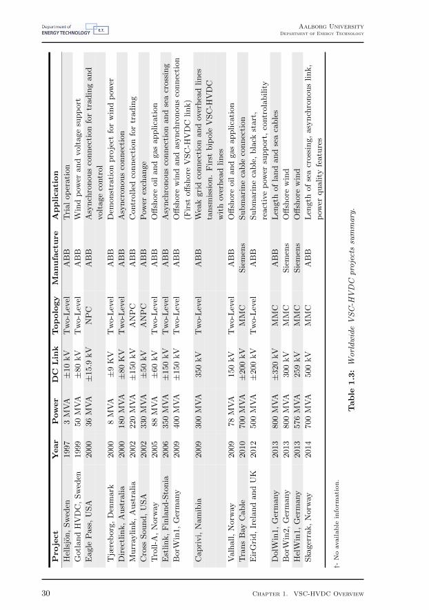
The increasing amount of VSC-HVDC projects in the world reflects the energymarket trend in integrating high power converters and DC transmission.
The key benefits and the competitive advantages presented previously canjustify such tendency. The niche of application for the mentioned convertersis broad, however, the offshore wind energy is the application which leads theamount of investments. Table 1.3 summarizes some of recent VSC-HVDC projectsworldwide and relates the applications.
Chapter 1. VSC-HVDC Overview 29
ii
“Thesis” — 2012/11/2 — 9:02 — page 30 — #30 ii
ii
ii
Aalborg UniversityDepartment of Energy Technology
Pro
ject
Year
Power
DC
Link
Topology
Manufactu
reApplication
Hel
lsjo
n,
Sw
eden
1997
3M
VA
±10
kV
Tw
o-L
evel
AB
BT
rial
op
erati
on
Gotl
and
HV
DC
,Sw
eden
1999
50
MV
A±
80
kV
Tw
o-L
evel
AB
BW
ind
pow
erand
volt
age
supp
ort
Eagle
Pass
,U
SA
2000
36
MV
A±
15.9
kV
NP
CA
BB
Asy
nch
ronous
connec
tion
for
tradin
gand
volt
age
contr
ol
Tjæ
reb
org
,D
enm
ark
2000
8M
VA
±9
KV
Tw
o-L
evel
AB
BD
emonst
rati
on
pro
ject
for
win
dp
ower
Dir
ectl
ink,
Aust
ralia
2000
180
MV
A±
80
KV
Tw
o-L
evel
AB
BA
syncr
onous
connec
tion
Murr
aylink,
Aust
ralia
2002
220
MV
A±
150
kV
AN
PC
AB
BC
ontr
olled
connec
tion
for
tradin
g
Cro
ssSound,
USA
2002
330
MV
A±
50
kV
AN
PC
AB
BP
ower
exch
ange
Tro
ll-A
,N
orw
ay2005
88
MV
A±
60
kV
Tw
o-L
evel
AB
BO
ffsh
ore
oil
and
gas
applica
tion
Est
link,
Fin
land-S
tonia
2006
350
MV
A±
150
kV
Tw
o-L
evel
AB
BA
synch
ronous
connec
tion
and
sea
cross
ing
BorW
in1,
Ger
many
2009
400
MV
A±
150
kV
Tw
o-L
evel
AB
BO
ffsh
ore
win
dand
asy
nch
ronous
connec
tion
(Fir
stoff
shore
VSC
-HV
DC
link)
Capri
vi,
Nam
ibia
2009
300
MV
A350
kV
Tw
o-L
evel
AB
BW
eak
gri
dco
nnec
tion
and
over
hea
dlines
tansm
issi
on.
Fir
stbip
ole
VSC
-HV
DC
wit
hov
erhea
dlines
Valh
all,
Norw
ay2009
78
MV
A150
kV
Tw
o-L
evel
AB
BO
ffsh
ore
oil
and
gas
applica
tion
Tra
ns
Bay
Cable
2010
700
MV
A±
200
kV
MM
CSie
men
sSubm
ari
ne
cable
connec
tion
Eir
Gri
d,
Irel
and
and
UK
2012
500
MV
A±
200
kV
Tw
o-L
evel
AB
BSubm
ari
ne
cable
,bla
ckst
art
,
react
ive
pow
ersu
pp
ort
,co
ntr
ola
bilit
y
DolW
in1,
Ger
many
2013
800
MV
A±
320
kV
MM
CA
BB
Len
gth
of
land
and
sea
cable
s
BorW
in2,
Ger
many
2013
800
MV
A300
kV
MM
CSie
men
sO
ffsh
ore
win
d
Hel
Win
1,
Ger
many
2013
576
MV
A259
kV
MM
CSie
men
sO
ffsh
ore
win
d
Ska
ger
rak,
Norw
ay2014
700
MV
A500
kV
MM
CA
BB
Len
gth
of
sea
cross
ing,
asy
nch
ronous
link,
pow
erquality
featu
res
†-N
oavailable
info
rmati
on.
Table
1.3:
Wo
rld
wid
eV
SC
-HV
DC
pro
ject
ssu
mm
ary
.
30 Chapter 1. VSC-HVDC Overview

ii
“Thesis” — 2012/11/2 — 9:02 — page 31 — #31 ii
ii
ii
Aalborg UniversityDepartment of Energy Technology
Pro
ject
Year
Power
DC
Link
Topology
Manufactu
reApplication
Mack
inac,
USA
2014
200
MW
70
kV
Tw
o-L
evel
AB
BIs
landed
op
erati
on,
volt
age
stabilit
y,
pow
erflow
contr
ol
INE
LF
E,
Fra
nce
-Spain
2014
2x1000
MV
A±
320
kV
MM
CSie
men
sU
nder
gro
und
cable
SylW
in1,
Ger
many
2014
864
MV
A±
320
kV
MM
CSie
men
sO
ffsh
ore
win
d
Sven
ska
Kra
ftnat,
Sw
eden
2014
1440
MV
AM
MC
Als
tom
Pow
erflow
contr
ol
Tre
sA
mig
as
2014
750
MV
AM
MC
Als
tom
Ener
gy
hub
Nord
Balt
,L
ithuania
-Sw
eden
2015
700
MV
A±
500
kV
MM
CA
BB
Len
gth
of
sea
cross
ing,
asy
nch
ronous
net
work
s
DolW
in2
2015
900
MV
A±
320
kV
MM
CA
BB
Len
gth
of
land,
sea
cable
s,
off
shore
win
d
Tro
llA
,N
orw
ay2015
100
MV
A±
60
kV
Tw
o-L
evel
AB
BL
ong
subm
ari
ne
cable
dis
tance
,
com
pact
nes
sof
conver
ter
Hel
Win
2,
Ger
many
2015
690
MV
A±
320
kV
MM
CSie
men
sO
ffsh
ore
win
d
†-N
oavail
able
info
rmati
on.
Table
1.4:
Wo
rld
wid
eV
SC
-HV
DC
pro
ject
ssu
mm
ary
-C
on
tin
ua
tio
n.
Chapter 1. VSC-HVDC Overview 31

ii
“Thesis” — 2012/11/2 — 9:02 — page 32 — #32 ii
ii
ii
Aalborg UniversityDepartment of Energy Technology
32 Chapter 1. VSC-HVDC Overview

ii
“Thesis” — 2012/11/2 — 9:02 — page 33 — #33 ii
ii
ii
CHAPTER2Introduction to Multiterminal
HVDC Systems
The applicability of DC transmission system and voltage source converters inthe modern power systems present their advantages and suitability, similarly
as it was outlined in previous chapter. For future trends, the interconnection ofmultiple VSC-HVDC stations is an envisage and has a backbone to the increasein the number of offshore wind farms which have been built and are planned fora near future (see tables 1.3 and 1.4).
The following text summarizes the concepts and challenges in MultiterminalVSC-HVDC (MTDC) technology. The principle of operation and possible layoutconfiguration are firstly explored. Challenges on the role of MTDC systems suchas protection and control issues are itemized lately. Final remarks regardingeconomic obstacles and prospects for supergrid concept are also briefly analysed.
2.1 General Description
The effects of the penetration of renewable energy has been felt by the Euro-pean power grid [2]. As main contributor for the modern energy market, the windenergy has been moving to offshore areas. The distances related with seaward landapplication, absence of reactive power compensation and size minimization of off-shore platforms, make the HVDC more competitive than the classical high voltageAC (HVAC) solutions.
Considering mainly the high penetration level of renewables, the connection ofthose geographically remote energy resources, located far from shore, their limitedcorrelation and their widely disperse distribution, the needs for the DC supergridsbecome potentialised.
The idea of supergrids is not new. The first proposal dates from 1930s, when,in the US, the creation of a long distance transmission network appeared. Theproject would drive the energy from the hydropowers linking the Pacific Northwest
33

ii
“Thesis” — 2012/11/2 — 9:02 — page 34 — #34 ii
ii
ii
Aalborg UniversityDepartment of Energy Technology
to the consumption areas located at the Southern California [24].
Meanwhile, this concept has become more and more mature by means of ad-vances in the electronics, control and cable technologies and, by 2001, its intendsfor the European unified power grid was launched. At that time, the intercon-nection among the existent power plants and the new generation from renewablesfrom wind in the north Europe and photovoltaic resources from South of Europeand Northern Africa was introduced. An extra benefit in balancing power appearsin the different time zones between east and west and the interconnected systemcan take advantages by strengthening the grid. Figure 2.1 illustrates the Euro-pean Supergrid map which integrates all the main energy resources from Europeby means of DC supergrid.
Figure 2.1: European DC supergrid map.Source: Friends of the supergrid.
Web: http://www.friendsofthesupergrid.eu/supergrid.aspx
2.2 Configurations
A multiterminal DC connection can be viewed as a link among three or moreHVDC converters. For the LCC based type, the control of parallel converterbecomes more troublesome, since the polarity of the DC voltage must change forpower flow reversal operation. This situation points the VSC-based HVDC as themost appropriate technology for supergrids concept for HVDC applications.
For the layout configuration viewpoint, the connection of converter for DCgrids can vary in number of interconnections and number of converters stations,depending on the dispersion of the load centers and generation zones. Though,one can group the layout in five main structures[25, 26]:
• Multiterminal with tappings;
• Grid with independent DC lines;
• Meshed DC grid;
34 Chapter 2. Introduction to Multiterminal HVDC Systems

ii
“Thesis” — 2012/11/2 — 9:02 — page 35 — #35 ii
ii
ii
Aalborg UniversityDepartment of Energy Technology
• DC grid with controllable devices;
• AC system connected by DC connections.
The first configuration (figure 2.2(b)) is the most simple multiterminal system.It is a radial connection and no redundancies are available. Topology could be usedas a very practical alternative for an AC connection. The proposed SouthWestLink (see tables 1.3 and1.4) is planed to be a multiterminal connection with radialconfiguration.
DC Grid
AC Grid
(a) Multiterminal with tap-pings
DC Grid
AC Grid
(b) Grid with independentDC lines
DC Grid
AC Grid
(c) Meshed DC grid
DC Grid
AC Grid
(d) DC grid with control-lable devices
DC Grid
AC Grid
(e) ACSystemConnectedby-DCConnections
Figure 2.2: Different DC grid topologies for potential supergrid application.
Figure 2.2(b) illustrates where all the buses are AC type. The AC lines werereplaced by DC with a point-to-point connection with two converter stationspromoting fully controllability of the power flow. This layout can operate withhybrid systems where LCC merges with VSC technology. The main advantagein such configuration is based on the fact that the AC protection system canbe incorporated. The number of converter is a troublesome in the mentionedinterconnection.
The following topology, the third (figure 2.2(c)), is a meshed DC grid. Thelinks can have or not have the presence of a converter station. It is the config-uration with the closest similarities from the classical AC systems. The inter-connected network supports redundancies since multiple paths are available. Thereliability and flexibility of meshed grids promote this kind of layout. However,the protection equipments are still not mature and is a limiting factor for itsdevelopment.
The composition among the meshed connection with additional converters(dotted lines connected by red dots) forms the layout presented in figure 2.2(d).Such devices can be connected by the AC side and series connected in the DClink. In one station, the combination can present LCC and VSC topologies atthe same time. With this merge, the power flow control can still be guaranteed
Chapter 2. Introduction to Multiterminal HVDC Systems 35

ii
“Thesis” — 2012/11/2 — 9:02 — page 36 — #36 ii
ii
ii
Aalborg UniversityDepartment of Energy Technology
but the losses and cost of the total converter station can be reduced. DC-to-DCconverter can also be included as candidate. However, for high power and highvoltage application, the cost of the devices is still the main issue.
The last configuration (figure 2.2(e)) represents the connection of AC gridsby means of DC. This configuration splits the AC systems in smaller segments.Such approach can limit the fault propagation and cascading blackouts as well aspower exchange among decoupled systems. It means that the operation of the ACsystems can be independently accomplished with mitigation of the propagatingdisturbances from one AC system to the others.
2.3 Challenges
The advantage in promoting high integration level of energy resources, asillustrated in figure 2.1, makes the multiterminal VSC-HVDC technology veryattractive by its efficiency. However, as a consequence of its youthfulness, severalchallenges related to technical as well as economic issues are still emerging. Someexamples of the drawbacks which the multiterminal VSC-HVDC technologies af-front nowadays are listed as follows:
2.3.1 Protection
One of the main obstacles in the growth of multiterminal DC systems is relatedto the DC overcurrent protection. The problem in DC networks lies in the absenceof current zero crossing combined with the low system impedance increase thecomplexity of the DC breaker elements.
In the case of point-to-point connection, the operation of voltage source con-verters during DC faults can be accomplished by the coordination of AC circuitbreakers and chopper resistors presented in the DC link [27].
Nonetheless, for MTDC application (mainly in meshed DC grids), this tech-nique meets its limitations [28] which is the low system impedance in the DC. Inthis scenario, the development of solid state DC circuit breakers [29] and VSCtopologies which enables the fault handling capability [30] are envisaged.
The necessity of fast and reliable DC circuit breaker for DC fault clearance inDC grid applications brought the appeal in development of the Modular HybridIGBT DC Breaker. Simplified circuit diagram is presented in figure 2.3.
During normal operation, the DC current flows through the bypass. At themoment of the fault, the auxiliary DC breaker starts switching and modulating theDC current. At the same time, the fast disconnecter is opened and the main DCbreaker extinguishes the current. As a final stage of the fault clearance procedure,the mechanical switch isolates the primary voltage across the main DC breaker.
The claims in such topologies lies in the fact that the losses of the hybridtopology of the modular DC breaker are reduced to the equivalent losses of a
36 Chapter 2. Introduction to Multiterminal HVDC Systems

ii
“Thesis” — 2012/11/2 — 9:02 — page 37 — #37 ii
ii
ii
Aalborg UniversityDepartment of Energy Technology
Main DC BreakerResidual DC
Current Breaker
Current Limiting Reactor
Auxiliar DC BreakerFast Disconnector
Figure 2.3: Simplified circuit diagram of the modular hybrid IGBT DC breaker [29].
pure semiconductor breaker and the opening time required by such circuitry is onthe range of 2 ms.
The second solution presented by fault handling in the meshed DC networksintegrates the modular multilevel converter topologies were briefly exposed in theprevious chapter (figure 1.2(d)).
Considering the combination of the low loss ratings and modularity of modularmultilevel converters, the hybrid solution makes use of hybrid modules to assemblethe converter cells. In this topology, series connected IGBT devices are assembledwith full bridge modules as illustrated in figure 1.3(d). During the faulted period,the proper control of the stack hybrid cells can change the polarity of the entireDC arm voltages and, by this means, control the flow of the converter DC current.
2.3.2 Communication
The communication requirements in a DC grid is still an opened issue, since itis related with the size, control architecture and measurement units of the network.Depending on the size and the number of interconnection, the communicationlinks can require very complex structures.
Three main communication levels are considered. The first one is related tothe reference power set points. For this purpose, the ratings in the communicationspeeds can be relatively slow, requiring lower bandwidth.
The second stage of communication level integrates the dynamic control ofpower systems for stability improvement such as power oscillation damping amongthe partners in the DC grid. The requirements for this application demandscoordination and high reliability in the communication links.
The protection schemes will rely in the communication in some applications.For these conditions, very fast coordination among the converter stations arenecessary. Higher bandwidth is needed due to the fact the transit periods forprotection issues are in the range of ms.
Chapter 2. Introduction to Multiterminal HVDC Systems 37

ii
“Thesis” — 2012/11/2 — 9:02 — page 38 — #38 ii
ii
ii
Aalborg UniversityDepartment of Energy Technology
2.3.3 Grounding
During a pole to ground fault type, the surge currents pass through ground.High or low impedance grounding schemes can be applied for reducing groundcurrents and assisting the protection scheme increasing the clearance time.
On the other hand, depending on the choice of the ground circuitry, while theground impedance is increased (as well the clearance time requirements) the polevoltage is boosted. With this increase, the converter voltage ratings and, as directconsequence, the final price of the converter station.
2.3.4 Operation
In case of a DC supergrid, more than one Transmission System Operator(TSO) is in charge of the control and coordination of the system. In the connectionwith many areas, the deregulated DC transmission system will require differenttypes of operation: coordinated operation, independent operation and integratedoperation [31].
In the coordinated control, as the same as it is presented by large multi-TSOpower systems, the need for a central MTDC TSO is essential. Having the securityassessment as a main purpose, the central controller defines the operation of theMTDC system based in the agreed TSO interests and benefits.
Ancillary services, such as primary frequency control, are handled. Due to theinterconnected scheme, the sharing of primary reserves and its control on timeassures that different reserves resources and their time period are satisfactory forall the partners.
For short-term power unbalances, which is applied in areas with limited re-serves resources, the HVDC TSO can operate the DC system with the aim ofsmoothing the changes in the power flow. The dynamic impact, resulting fromthe fast changes in the interconnected areas, can be handled.
By considering the independent operation, the HVDC TSO handles the con-verter and line loadings according to its revenue maximisation. The operationis similar to the generation policies where the rewards are counted by providingreserves where they are more profitable, based in connection and economic rules.
Compared with the coordinated condition, this operation mode allows moredeviations with regards to power deviations.
The operation mode considers the integrated operation of the DC system.It is assumed that the TSOs of some areas can manage the converter stations,the loading of lines and cables. In this situation, the TSOs are able to supporttheir own AC systems as well as support the operational costs. In this case,the agreements in negotiating ancillary services among partners rely on technicalflexibility and in the policies of interdependencies among the many partners.
38 Chapter 2. Introduction to Multiterminal HVDC Systems

ii
“Thesis” — 2012/11/2 — 9:02 — page 39 — #39 ii
ii
ii
Aalborg UniversityDepartment of Energy Technology
2.3.5 Control
Considering the MTDC control of power, the DC voltage compensation playsan important role in promoting the full flexibility of the MTDC in the sharingof power. Four main control strategies have been studied as the most suitablecandidates for multiterminal VSC-HVDC transmission systems [32, 33, 34].
• Voltage droop
• Ratio control
• Priority control
• Voltage margin method
2.3.5.1 Voltage Droop
Similarly to the frequency control in AC systems, where the dependency ofthe load and frequency is used as an effective adjust the generator power of syn-chronous machines, in MTDC applications, the droop control regulates the DCvoltage according to the receiving power for balancing enforcement.
The maximum and minimum values for the DC voltage are set and, dependingon the level of the DC current/power, the set point of the converter voltagereference can drop or increase according to the slope θ of the droop curve. Theoperation of the converter as rectifier or inverter is dependent of the DC voltagelevel as shown in figure 2.4.
VDCV*
VMinV*
VMaxV*
1pu
+1pu-1puRectifier Inverter IDC
PDC
θ
Figure 2.4: Example of DC droop curve for multiterminal DC applications.
2.3.5.2 Ratio Control
The ratio control is a special case of droop control where the DC voltage droopfactors are applied just in the inverter end stations. The receiving end station isable to share the power from the sending end terminals depending on the definedrelationship among the droop factor applied in the voltage controllers. Figure 2.5illustrates an example of a droop curve for the ratio control scheme.
Chapter 2. Introduction to Multiterminal HVDC Systems 39

ii
“Thesis” — 2012/11/2 — 9:02 — page 40 — #40 ii
ii
ii
Aalborg UniversityDepartment of Energy Technology
VDCV*
VMinV*
VMaxV*
+1pu-1puRectifier Inverter IDC
PDC
θ1
θn
Figure 2.5: Example of DC droop curve for multiterminal DC applications using ratiocontrol.
2.3.5.3 Priority Control
In this control mode, one of the converters in the DC link has priority in thepower transfer. This terminal has the direct DC voltage control and, as soonas the processed power reaches the set point, established by the operation rules,the DC voltage regulator has no longer capability for maintain the DC voltagebalance which will increase as a consequence of increasing in power. Thus, theother terminals in the link start to process power once the converter in whichthe priority was included reached its limits. The curve presented in figure 2.6illustrates an example of a priority control droop curve.
VDCV*
VMinV*
VMaxV*
+1pu-1puRectifier Inverter IDC
PDC
θ
VDC
Figure 2.6: Example of DC droop curve for multiterminal DC applications using pri-ority control.
2.3.5.4 Voltage Margin
The voltage margin method combines the power and direct voltage controlmodes. A voltage margin is given to each of the converter connected to the DCgrid. This margin is defined as a maximum and minimum values in which rangethe DC bus voltage reference can deviate. By changing the limits of the DCvoltage regulators according to the power set point, the maximum and minimumvalues of the DC voltage compensation defines the operation of the converter asrectifier or inverter modes. Figure 2.7 gives an example for a system that adopts
40 Chapter 2. Introduction to Multiterminal HVDC Systems

ii
“Thesis” — 2012/11/2 — 9:02 — page 41 — #41 ii
ii
ii
Aalborg UniversityDepartment of Energy Technology
the voltage margin method.
VDCV*
VMinV*
VMaxV*
1pu
+1pu-1puRectifier Inverter IDC
PDC
VDCV*
Figure 2.7: Example of voltage margin curve for multiterminal DC applications.
2.3.6 Standardisation
As an immature but with high potential technology, multiterminal VSC-HVDC does not experience, nowadays, any effort in standardisation such as DCvoltage levels and compatibility, as already presented in AC power systems. Dif-ferent manufacturers are today in the market, and with the prospects in growingand matureness, more competition and parties can appear in the increasing sce-nario.
At this moment, no real standards for DC voltage levels, for example, are inoperation. From table 1.3, it is possible to verify that there is no accordancein the DC bus voltage levels among the released and the new projects to becommissioned. This first issue can bring many challenges in the future prospectsin interconnecting all those established systems.
The different converter topologies, protection schemes, operation and controlstrategies adopted by the manufactures can interact. The effects in one into theother can be unsuitable when the prospects in integrating all those system in areal meshed MTDC power system.
2.3.7 Economics
The technical benefits of having an interconnecting DC system is a clear ad-vertising for MTDC due to lower losses, high distance transmission using cabletechnologies and power flow control flexibility, mainly considering the market ofrenewable resources.
In some applications, the HVDC transmission appears as an unique solutionfor power transmission. One example is the offshore wind application, remotelyconnected by means of submarine cables. In this case, the AC interconnectionbecomes costly enough to overtake the high cost off HVDC converter stations.
However, when the use of multiterminal HVDC to reduce the congestion intransmission capacity is taken into account, the necessary investments in build-
Chapter 2. Introduction to Multiterminal HVDC Systems 41

ii
“Thesis” — 2012/11/2 — 9:02 — page 42 — #42 ii
ii
ii
Aalborg UniversityDepartment of Energy Technology
ing such infrastructure are nowadays doubtful. The competition with the wellestablished and reliable AC transmission systems and its cost make the super-grid concept unsure. Significant investments are essential and require multipleinvestors. For such, the positive return and acceptable pay-back time is dubiousand undetermined.
2.3.8 Supergrid Foresee
The multiterminal connection of VSC-HVDC transmission system (the pioneerof the supergrid) is a growth but still immature technology. There is no systemsat the moment and its commissioning will be predicted to the following years tocome. The DC supergrid formed by the interconnection of multiple voltage sourceconverters in a meshed layout is even more futuristic.
Many technical and politic/economic issues are still opened. However, thecurrent developments in the HVDC technologies make the supergrid a possiblescenario for the future of transmission power system.
42 Chapter 2. Introduction to Multiterminal HVDC Systems

ii
“Thesis” — 2012/11/2 — 9:02 — page 43 — #43 ii
ii
ii
CHAPTER3Control Optimisation in
Multiterminal VSC-HVDC
The selected method to control the power flow in multiterminal HVDC is basedon DC voltage droop in each of the converter stations in which the DC voltage
controllers are enabled. Considering the back-to-back wind generation convertertype and AC collector for offshore connection, the droop controls applied in theonshore stations are able to define the appropriate voltage levels for a desiredpower dispatch. Moreover, using such an approach, it is possible to have morebuses in which the DC voltage can be controlled, bringing more flexibility forlarge DC networks.
This chapter is focused in the design of the droop factors for DC networks andthe optimisation methods to select the proper values for the reference set pointsare introduced. The constrained optimisation scenarios are listed and they arepresented in study cases for loss minimisation and two cases involving dispatchmaximisation problem.
3.1 Optimisation Objectives
In layman’s terms, an optimisation problem consists in finding the best pointof a function, considering maximum or minimum conditions, for the set of itsfeasible solutions. A more restrict issue appears when constraints are included inthose conditions, narrowing down, even more, the solution group.
The general mathematical model for such problem is represented by (3.1).
minimise fo (x) (3.1)
subject to fi (x) ≤ 0, i = 1, 2, 3, . . . ,m
In (3.1), x is the optimisation variable (or decision variable) with n compo-nents. The function fo : Rn → R, is the objective function, the one in which max-imum or minimum requirements are placed. fi : Rn → R are the m constraints.
43

ii
“Thesis” — 2012/11/2 — 9:02 — page 44 — #44 ii
ii
ii
Aalborg UniversityDepartment of Energy Technology
Whether the optimum solution of the objective function under the constraintsconditions is feasible, this point is specified by x∗ and fo (x∗) is the critical point.
Based on the properties of the objective function and its constraints, the com-plexity in finding the solution fo (x∗) can considerably vary. In order to overtakethis bottleneck, a solution method for many of the optimisation problems can bereleased by computer based algorithms where the critical points, when feasible,are numerically obtained. Many of these tools are available today and they differon the complexity and effectiveness in finding the solution [35].
The method adopted for further development is called interior point. Alsoknown as barrier method, this algorithm, roughly speaking, changes a complexproblem summarized by the framework given by (3.1) into a simpler one, justadding a dual function in the objective function such as is written in (3.2).
minimise fo (x) + Φ (x) (3.2)
The graphical representation of the dualisation method is shown in figure 3.1,where a modulus function (continuous blue line) is firstly approximated by asecond order polynomium (dashed red line) and by a sixth order polynomium(dotted black line).
−1 −0.5 0 0.5 10
0.2
0.4
0.6
0.8
1
1.2
1.4Original functionDual function #1Dual function #2
Figure 3.1: Graphical representation of an optimisation problem dualisation.
The original objective function fo (x) is represented by the continuous blueline in figure 3.1. Due to the conner at the origin, no feasible solution can befound, since the derivatives in that point vanish. However, approximating fo (x)to a second order polynomium (red dotted line), the new function is differentiable.Increasing the the order of polynomium, the new function is represented by theblack dashed function in figure 3.1. Higher the order of the polynomium, higheris the accuracy of the approximation.
The objective of the algorithm is, then, to change the value of a parameter ofa dual function which is completely differentiable (in the current case, the orderof a polynomium that best fits the original objective function). The critical pointof such dual function can be found using regular linear optimisation methods likeNewton’s Method or even analytical methods.
For the general problem presented by (3.1), the dualisation is taken by repre-
44 Chapter 3. Control Optimisation in Multiterminal VSC-HVDC

ii
“Thesis” — 2012/11/2 — 9:02 — page 45 — #45 ii
ii
ii
Aalborg UniversityDepartment of Energy Technology
senting Φ (x) in (3.1) using the sum of the logarithm of the constraints (3.3).
Φ (x) = −1
t
m∑
i=1
log (−fi (x)) (3.3)
where t is the changeable parameter. Higher the value of t, closer the dual objec-tive function is to the original one. As an illustrative example, it is possible toverify the variation of the parameter t in a optimisation problem by looking intofigure 3.2.
x1
x2
x = xot = to
fo (x) + Φ (x)f1 (x)
f2 (x)
0 0.2 0.4 0.6 0.8 10
0.2
0.4
0.6
0.8
1
(a) Step 1
x1
x2
x = xot = to
x = x1t = t1
fo (x) + Φ (x)f1 (x)
f2 (x)
0 0.2 0.4 0.6 0.8 10
0.2
0.4
0.6
0.8
1
(b) Step 2
x1
x2
x = xot = to
x = x1t = t1
x = x2t = t2
fo (x) + Φ (x)f1 (x)
f2 (x)
0 0.2 0.4 0.6 0.8 10
0.2
0.4
0.6
0.8
1
(c) Step 3
x1
x2
x = xot = to
x = x1t = t1
x = x2t = t2
x = x3t = t3
fo (x) + Φ (x)f1 (x)
f2 (x)
0 0.2 0.4 0.6 0.8 10
0.2
0.4
0.6
0.8
1
(d) Step 4
Figure 3.2: Representation of the path taken by the optimum point for variation in theparameter t.
In the first iteration, an optimum point to the function fo (x) + Φ (x) is foundat x = xo for parameter value t = to (figure 3.2(a)).
Second, a new parameter t = t1 is chosen such that t1 = µto, for µ > 1. Anew optimum point x = x1 is found (figure 3.2(b)). The tolerance ε is checkedby verifying the difference between xo and x1. The same procedure is taken inthe steps 3 and 4 (figures 3.2(c) and 3.2(d)). However, in the step 4 the iterativeloop stops since the tolerance is achieved. Algorithm 1 summarizes the procedurepresented in figure 3.2.
Chapter 3. Control Optimisation in Multiterminal VSC-HVDC 45

ii
“Thesis” — 2012/11/2 — 9:02 — page 46 — #46 ii
ii
ii
Aalborg UniversityDepartment of Energy Technology
Algorithm 1 Interior point algorithm
Given a initial parameter value t = t0, µ > 1 and tolorence ε > 0repeat
Compute x∗ which minimises fo (x) + Φ (x)Update the value of x by x = x∗
Increase the value of t by t = µtuntil m
t< ε
3.2 Application of Optimisation in Droop FactorDesign: Study Cases
The selection of the droop gains for DC networks by means of optimisationcan assess many objectives. Considering the static viewpoint, some of them canbe mentioned. The first one is to select the values of the droop controllers in orderto decide for appropriate voltage levels, aiming to achieve minimum transmissionlosses. For the same scenario, quantification of the converter losses can be alsoincluded in the model.
Another possible solution can be related with the optimisation in the powerdelivered to the AC grids connected to the DC transmission system. By doingthat, the error in the dispatch can come into picture and can characterize theobjective function.
For the determination of droop factors using one of the previous cited scenar-ios, a general procedure is adopted. However, the test benchmark for evaluationproperties consider a DC grid formed by two onshore stations and two offshorestations connected to offshore wind farms as illustrated in figure 3.3.
#3
AC1 #1
#2
AC2#4
WPP1 WPP2
200km 100km100km
400MW 200MW
400MW 200MW
Figure 3.3: Multiterminal VSC-HVDC benchmark employed in the optimisation anal-ysis.
Voltage and nominal power for each of the converter stations are summarizedby table 3.1.
1 2 3 4
DC Voltage ±150kV ±150kV ±150kV ±150kVDC Power 400MW 400MW 200MW 200MW
Table 3.1: System nominal parameters.
46 Chapter 3. Control Optimisation in Multiterminal VSC-HVDC

ii
“Thesis” — 2012/11/2 — 9:02 — page 47 — #47 ii
ii
ii
Aalborg UniversityDepartment of Energy Technology
Cable lengths and impedance per kilometer are presented in table 3.2
Bus from Bus to Distance [km] Impedance[
Ωkm
]1 2 200 0.01762 3 100 0.03663 4 100 0.0366
Table 3.2: Cable lengths and impedances.
Clearly, the power flow in the system from figure 3.3 is driven by the voltagedifference among the DC buses. Compared with classical AC connection, thesystem is more restrictive. In sinusoidal operation, two degrees of freedom areavailable for power transfer control properties: voltage difference and phase angle.Changing both variables, active and reactive power are transferred from one busto the other.
However, one degree of freedom is lost in a DC network, which means thatonly active power is available. This fact can be seen as a simplification for thesystem load flow calculation and, on the other hand, an increase in the controleffort to keep the stability or system performance.
Considering, first of all, the static scenario, the power flow can be analysed.Using the load flow calculation, voltage and power in each of the converter stationscan be predicted [36]. As a result, the set points for the converter controllers areset and, indirectly, the droop factors can be derived. At this point, the mentionedset points are calculated using load flow. In the next chapters, the droop factorsare going to be analysed since dynamic models are presented and variations areconsidered.
Two main cases are included in the load flow calculation and each of them aresplit in two more cases. They are listed as follows:
1. Loss minimisation
(a) Cable loss minimisation
(b) Cable and converter loss minimisation
2. Dispatch optimisation
(a) Dispatch error minimisation
(b) Power delivery maximisation
In all of the cases, the main core of the load flow is the definition of theobjective function in the framework presented in (3.1). The procedure is similarin all the scenarios. Due to that, the methodology is deeply explored in the lossminimisation case and repeated in the other items.
To define the set point values in a DC network such method can be appliedin the DC load flow problem. Advantage of this implementation is that none ofthe buses are treated specially such a slack bus. Besides all the voltage levels inall the buses in the system can be properly chosen since the objective function isoptimized and the constrains are satisfied.
Chapter 3. Control Optimisation in Multiterminal VSC-HVDC 47

ii
“Thesis” — 2012/11/2 — 9:02 — page 48 — #48 ii
ii
ii
Aalborg UniversityDepartment of Energy Technology
3.2.1 Loss Minimisation
3.2.1.1 Cable Loss Minimisation
The problem in minimising the DC transmission losses is the simplest caseto be presented. In some real cases, the losses in the system can justify itsapplication [?]. Despite the fact that it does not consider some main requirementsfor the grid, it can be seen as a starting point to build more general strategies.Additionally, this is an evaluation tool to verify the operational aspects of theoptimisation.
Considering the test system from figure 3.3, for the load flow analysis thesystem can be simplified considering just the nodes and branch impedances asillustrated in Figure 3.4.
#3
#1
#2
AC2
#4
WPP1 WPP2
AC1
R12 R23 R34
Figure 3.4: Simplified circuit for DC load flow analysis.
In figure 3.3, the impedances are represented by cable resistances and twotype of buses are considered. The ones where the DC voltage control is enable arerepresented by voltage sources. The infeed points, which are the HVDC stationswhere the wind farms are connected, are represented by current sources. TheHVDC converter that is in active power mode control can also be represented bythis model.
The node voltage are V1, V2, V3 and V4 and the currents I12, I23 and I34 flowthought the terminals of the resistors R12, R23 and R34 driven by the node voltagedifferences. The currents in each of the branches are written as follow:
I12 =V1 − V2
R12(3.4)
I23 =V2 − V3
R23(3.5)
I34 =V3 − V4
R34(3.6)
Using vectorial notation, the currents can be grouped as i = [I12I23I34]T
. Forthe case of loss optimisation, the cost function J(.) can be written as presented
48 Chapter 3. Control Optimisation in Multiterminal VSC-HVDC

ii
“Thesis” — 2012/11/2 — 9:02 — page 49 — #49 ii
ii
ii
Aalborg UniversityDepartment of Energy Technology
in (3.7).
J (vDC) = vTDC ·Y · vDC (3.7)
where vDC is the DC voltage vector and its elements are the voltages at eachstation in the network and Y is the admittance matrix formed by the branchconductances of the DC cables. The superscript .T indicates the vector transposeoperation.
The admittance matrix can be written following (3.8).
YDC,ij =
−yDC,ij if i 6= j∑Nj=1 yDC,ij if i = j
(3.8)
where yDC,ij is the conductance between the buses i and j and N is the numberof buses. Due to the way in which the admittance matrix is built, it is possibleto assure that YDC is symmetric.
As a constrained optimisation problem, since the network equation must besatisfied, (3.9) can be written.
g (vDC ,pDC) = Y · vDC + (diag (vDC))−1 · pDC = 0 (3.9)
where pDC is the power processed by each bus and diag (vDC) the diagonal matrixformed by the values for the DC voltages. This power vector contains the constantcomponents of power, that are generated by the wind farms pDCWPP
, and theones pDCD
which are going to be calculated during the load flow analysis anddelivered to the AC grids.
It should also be considered the physical limitation of the system into the vec-tor vDC by means of considering the voltage boundaries, which means write (3.10).
vminDC ≤ vDC ≤ vmaxDC (3.10)
The power limits should also be considered as constraints. Two main purposesare related to this topic. The first one is the limitation of the the DC cables andthe second case is related with converter ratings. It is going to be considered thatthe power ratings of the cables are the same presented by the converters in whichthe power is delivered to the grid. So, similar to (3.10), the power vector limitsare written according to (3.11).
pminDC ≤ pDC ≤ pmaxDC (3.11)
The power limits can be set differently from the system limits. The powerbounds are going to drive the system to the power control mode during the oper-ation. Moreover, it is possible to the converter operates in a bidirectional modemeaning that the onshore station is injecting power in the grid. In this condition,the same limitation for the bounds can be applied, however the signal of the powervector elements must be changed from positive to negative.
Chapter 3. Control Optimisation in Multiterminal VSC-HVDC 49

ii
“Thesis” — 2012/11/2 — 9:02 — page 50 — #50 ii
ii
ii
Aalborg UniversityDepartment of Energy Technology
Taking into account, first of all, the optimal voltage vector v∗DC , the optimalsharing condition distribution p∗DCD
is inside the set formed by cost function andconstraints as showed above. The following Lagrangian function can be expressed.
L(vDC ,pDCD
,λ)
= J (vDC) + g (vDC ,pDC) · λT (3.12)
and λ are the Lagrangian multipliers for the constrained optimisation problemgiven by (3.12).
Since the seeking for candidates for critical points are inside the boundedregion, where the partial derivatives of (3.12) can be computed, the first order-necessary optimability conditions are (3.13), (3.14) and (3.15).
∂L(vDC ,pDCD
,λ)
∂vDC= 0 (3.13)
∂L(vDC ,pDCD
,λ)
∂pDCD
= 0 (3.14)
∂L(vDC ,pDCD
,λ)
∂λ= 0 (3.15)
For this propose, just the components pDCDare taken into account because
the power from the wind farm is considered to be constant.
Deriving (3.13), (3.14) and (3.15), it is possible to obtain:
2 ·YDC · vDC − (diag (vDC))−2 · pDC · λT = 0 (3.16)
(diag (vDC))−1 · λ = 0 (3.17)
(diag (vDC))−1 · pDC = 0 (3.18)
Considering what (3.16), (3.17) and (3.18) show, the interior region belong-ing to the constrained and bounded problem given by (3.12) does not containthe minimum for the problem since the equations converge to conditions wherethe voltages are all zero. Assuming that (3.7) is convex, the minimum presentedby (3.16), (3.17) and (3.18) shows a unique global solution. Figure 3.5(a) illus-trates this problem.
With this conclusion in hands, there are more two conditions where it is pos-sible to find the solution: the boundaries and the corners. Considering a generalcase where the vector variable is x, when the boarders (inequality constraints) ofthe domain are taken into account, the derivatives vanish due to discontinuitiesand the equations given by (3.12) are not valid anymore. It means that the globalcritical point x∗ does not belong to the bounded region and a local critical pointx∗Local is found instead. The algorithm starts by seeking for critical points fromthe initial condition xo and the boundaries, given by inequality constraints. Fig-ure 3.5(b) brings the description of evaluating optimisation problems in boundedregions.
50 Chapter 3. Control Optimisation in Multiterminal VSC-HVDC

ii
“Thesis” — 2012/11/2 — 9:02 — page 51 — #51 ii
ii
ii
Aalborg UniversityDepartment of Energy Technology
0 0.2 0.4 0.6 0.8 10
0.2
0.4
0.6
0.8
1
GlobalMinimum
1Minx 1
Maxx
2Minx
2Maxx
Constrained Region
LocalMinimum
2x
1x
(a) Simplified diagram to compare theinfluence of constraints in a optimisa-tion problem.
0 0.2 0.4 0.6 0.8 10
0.2
0.4
0.6
0.8
1
GlobalMinimum
1Minx 1
Maxx
2Minx
2Maxx
Constrained Region
LocalMinimum
2x
1x
Starting Point
AlgorithmPath
(b) Influence of constrains in the opti-misation algorithm.
Figure 3.5: Representation of constraints in an optimisation problem.
Analysing the problem from (3.7) with the constraints (3.9), (3.10) and (3.11),the equality constraint, given by the network equation, and the inequality con-straints given by the voltages and power limits, play an important role in findingthe solution for the problem of losses minimisation. When choosing to stay onthe line of the boundary, one degree of freedom is lost and the analysis usingLagrangian can be used again. However, the new vector has less one dimension.
Considering the loss optimisation case from figure 3.4, and it is possible toinfer that the voltage at bus number 2 will be guided to the highest voltage levelcompared to the other buses. Choosing this bus for fixing the voltage level atone of the limits, the new equations for the objective function and the equalityconstraint becomes:
J (vDC) = vTDC · Y · vDC (3.19)
g (vDC , pDC) = Y · vDC + (diag (vDC))−1 · pDC (3.20)
where . is new vector or matrix with less one element in case of a vector, or linein case of a matrix.
The inequality constraints, given by the voltage limitation, are written asfollows:
vminDC ≤ vDC ≤ vmaxDC (3.21)
With less one degree of freedom, the Lagrangian equations can be appliedagain. For all the boundaries this checking must be considered. For the currentsystem, four buses are available and 2 voltage limits per bus must be examined.For N buses, 2N boundaries must be checked. For meshed DC grids, it is possibleto find more cases where the DC limits are achieved, and once more, the numberof degrees of freedom is decreased. After checking of all the boarders, the checkingin the corners come into picture. In the end, all of these results are put togetherand the minimum is selected.
Chapter 3. Control Optimisation in Multiterminal VSC-HVDC 51

ii
“Thesis” — 2012/11/2 — 9:02 — page 52 — #52 ii
ii
ii
Aalborg UniversityDepartment of Energy Technology
For the loss minimisation case, the mathematical model, using the frameworkfrom (3.1), can be written according to (3.22).
minimise vTDC ·Y · vDC (3.22)
subject to Y · vDC + (diag (vDC))−1 · pDC = 0
vminDC ≤ vDC ≤ vmaxDC
pminDC ≤ pDC ≤ pmaxDC
For the case presented in figure 3.4, there are six unknowns, the voltage valuesin the buses and the power shared by each onshore grid. For the equality con-straints, three equations are derived from the node equation and they take intoaccount the power balanced processed by the network.
The analytical solution presented above can be archived using the calculationof the Lagrangian function. However, for big systems it becomes not practicalallowing the interior point algorithm to be used. Other methodologies are alsoavailable today. Examples of algorithms, besides interior point, are trust regionreflective and active set. More advanced techniques are still in development andthey apply genetic algorithms, neural networks and fuzzy logic.
The optimisation algorithm and the load flow analysis are related accordingto the flow diagram presented in the chart 2.
Algorithm 2 Optimized DC load flow algorithm for calculating operating pointsin DC networks
Require: Inputs:
# of buses: N +MType of buses: 1 or 2Power of Injection: PM
Cable impedances: ri,j
Require: Variables Initialization:
Vn = 1.0Vm = 1.0error = 1.0tolerance = 1.0e-9
function Y-Bus Creation(YBus)Equation (3.8)
end functionInitialization of the optimisation vector: x = [V1, . . . , VN+M , P1, . . . , PN ]function Optimization(x)
Determine a direction ∆xObjective function calculation: J(x) . Required input J(x)Line searchUpdate xif Constraints satisfied are not satisfied then returnend if . Required input g(x)
end functionUpdate network variables
Implementing the algorithm presented in Figure 2, the results for the DCvoltages values are presented in Figure 3.6.
Figure 3.6 shows the dashed lines illustrating the allowed region of variation of±3%. As expected, the voltage levels on the infeed points (the buses where there
52 Chapter 3. Control Optimisation in Multiterminal VSC-HVDC

ii
“Thesis” — 2012/11/2 — 9:02 — page 53 — #53 ii
ii
ii
Aalborg UniversityDepartment of Energy Technology
1 2 3 40.97
0.98
0.99
1
1.01
1.02
1.03
Bus Number
DC
Voltage
Figure 3.6: DC voltage profile in the DC network.
are power injection from the wind farms) achieve the maximum allowed values.On the other buses, they assume similar values as consequence of the minimisationof the objective function. For the power distribution, the measurements presentedby the simulation is showed in Figure 3.7.
1 2 3 40
0.05
0.1
0.15
0.2
0.25
0.3
0.35
Bus Number
DC PowerAC Power
(a) Processed Power
1 2 3 4 50
0.002
0.004
0.006
0.008
0.01
#1 #2
#3 #4
Cable
(b) Power Losses
Figure 3.7: Power distribution for the transmission loss minimisation.
The results presented by figure 3.7 show the possibilities and the explanation ofoperation of a DC network using DC voltage droop. However, just one operatingpoint was considered. One can infer what are the conditions which are goingto define the control signals for different operating points. The variability of theinjected wind power and the different conditions of cable impedances can be takeninto account.
For the power variation case, it is aimed to verify what are going to be voltageprofiles for different wind conditions. The behaviour described by figure 3.8 showsthe tendency of the system in maintaining the symmetry since the voltages in theterminal buses decrease at same ratings for variation in the wind farm production.
For the power and losses distribution, considering the delivered power fromthe wind power plants and the infeed powers injected in the AC grids, the resultsare showed in Figure 3.9.
Equations derived above to define the optimum DC load flow for transmissionloss minimisation are related with the voltages at the DC buses and the system
Chapter 3. Control Optimisation in Multiterminal VSC-HVDC 53

ii
“Thesis” — 2012/11/2 — 9:02 — page 54 — #54 ii
ii
ii
Aalborg UniversityDepartment of Energy Technology
1 2 3 4
0.98
1
1.02
1.04
1.06
Bus Number
DC
Voltage
WPP1 = 100MW , WPP2 = 100MWWPP1 = 200MW , WPP2 = 100MWWPP1 = 250MW , WPP2 = 100MWWPP1 = 250MW , WPP2 = 150MW
Figure 3.8: Voltage profile variation in case of modification of wind power set points.
1 2 3 40
0.1
0.2
0.3
0.4
0.5
0.6
0.7
Bus Number
WPP1 = 100MW , WPP2 = 100MWWPP1 = 200MW , WPP2 = 100MWWPP1 = 250MW , WPP2 = 100MWWPP1 = 250MW , WPP2 = 150MW
(a) Processed Power
1 2 3 4 50
0.002
0.004
0.006
0.008
0.01
0.012
0.014
#1#2
#3 #4
Cable
(b) Power Losses
Figure 3.9: Power distribution for the transmission loss minimisation.
characteristic given by branch impedances. The power flow results as consequenceof the those variables. With this information in hands, a verification of the in-fluence of cable variation over the voltage profile and power distribution can beintended.
Considering that the cable impedance of the branch with connects the off-shore wind farm at bus number 2 to the land, thought bus number 4 changes itsimpedance from the minimum value of 100km, and assuming the values 175kmand later achieving the maximum values of 250km, figure 3.10 shows a variationof impedances and how the voltage profile and power distribution are affected.
As the same as the previous results presented a symmetric variation of thevoltage profile, the algorithm for the DC load flow based on transmission lossesminimisation varies the onshore bus voltages with the same portion. The powerinstead, varies accordingly, flowing to the branches were the impedances are lower.
Observing the results, for a DC network, the classical load flow can be used andthe choice of slack buses must be included, since the system presents more degreesof freedom than equations. However, the scenario is suitable for optimisation toolsand, besides the fact that the algorithms can provide the load flow analysis, theyare able to bring more flexibility.
A method based on the loss minimisation was analysed and its behaviour under
54 Chapter 3. Control Optimisation in Multiterminal VSC-HVDC

ii
“Thesis” — 2012/11/2 — 9:02 — page 55 — #55 ii
ii
ii
Aalborg UniversityDepartment of Energy Technology
1 2 3 4
0.98
1
1.02
1.04
1.06
Bus Number
DC
Voltage
d12 = 100kmd12 = 125kmd12 = 150kmd12 = 175kmd12 = 200km
(a) Voltage profile
1 2 3 40
0.1
0.2
0.3
0.4
0.5
Bus Number
d12 = 100kmd12 = 125kmd12 = 150kmd12 = 175kmd12 = 200km
(b) Power distribution
1 2 3 4 50
1
2
3
4
5
6
7
8x 10
−3
#1 #2
#3#4
Cable
(c) Loss distribution
Figure 3.10: System behaviour under cable impedance variation for transmission lossesoptimisation case.
wind power injection variation and changes in the cable impedances were verified.For this approach, however, the power flow is a consequence of the parametersof the system, characteristic that can not be so tight in real applications since itis necessary to have the proper control of power or, at least, to control how thetotal power is shared among the stations connected in the DC link.
3.2.1.2 Total Loss Minimisation
The previous method showed an objective function based on the transmissionlosses in the DC link. However, one can consider to calculate the losses of thesystem and include the converter losses in the objective function. For the presentcase, the losses to be considered are the phase reactor losses and converter losses.Converter losses take into account the conduction losses and switching losses ofthe IGBT [38].
The phase reactor losses PL,Reactor are calculated using (3.23).
PL,Reactor = 3 rReactorI2RMS (3.23)
where rReactor is the phase reactor impedance and IRMS is the RMS value of the
Chapter 3. Control Optimisation in Multiterminal VSC-HVDC 55

ii
“Thesis” — 2012/11/2 — 9:02 — page 56 — #56 ii
ii
ii
Aalborg UniversityDepartment of Energy Technology
current through the reactor.
For the IGBT losses, two kind of losses are taken into account: the switchinglosses and conduction losses. For the following calculations, a basic linear lossmodel for power semiconductors is assumed. It means that, during each switchingperiod, the voltage and current in the valve will follow a ramp curve during theincreasing or decreasing conditions.
The equation of the switching losses of a VSC with sinusoidal AC line currentand with IGBT switching devices is given by equation (3.24).
PSw =6
πfsw (EON,IGBT + EOFF,IGBT + EOFF,D)
VDCVr
ioir
(3.24)
where, fsw is the switching frequency, EON,IGBT + EOFF,IGBT + EOFF,D is thesum of turn-on and turn-off energies in the power modules, VDC is the DC linkvoltage, io is the peak value of the AC line current and Vr and ir are the blockingstate voltages and currents occurring before the corresponding commutation. Forthe entire grid cycle, the sum of values calculated by (3.24) gives the averagevalues for the losses.
For the conduction losses, the equation for calculation of it is given by (3.25).
PC = 6
((VCE + VF ) io
2π
∫ π
0
sin (ωt)1 +m(t)
2d (ωt) + . . .
(rCE + rF ) i2o2π
∫ π
0
sin2 (ωt)1 +m(t)
2d (ωt)
)(3.25)
where VCE and VF are the IGBT and diode threshold voltage, rCE and rF the dif-ferential resistances and m(t) is the modulation function give by equation (3.26).
m(t) = M sin (ωt) +3√
3
8π
∞∑
k=0
(sin (3 (4k + 1)ωt)
18k2 + 9k + 1− . . .
sin (3 (4k + 3)ωt)
18k2 + 27k + 1
)(3.26)
For this loss minimisation case, the upgraded cost function must present theprevious equation, given by the total DC transmission losses, and added now withthe factors given by equations (3.24) and (3.25). The phase reactor losses will notbe taken into account since it will drive the results to minimum power transmissionwhich is not desired. Proceeding on the same way as mentioned before for thetransmission loss minimisation case, the cost function can be defined accordingto (3.27).
J (vDC) = vTDC ·Y · vDC + (PC + PSw) (3.27)
Once more, the values for the DC voltage and the power delivered to theAC grids are the aims. At this time, a more complicated function is considered
56 Chapter 3. Control Optimisation in Multiterminal VSC-HVDC

ii
“Thesis” — 2012/11/2 — 9:02 — page 57 — #57 ii
ii
ii
Aalborg UniversityDepartment of Energy Technology
since the vector PC and PSw, always positive, related with the power losses ineach converter station are taken into account in the optimisation loop. The sameconstraints are still used.
As soon as the values for PC and PSw are inserted in the object function, morecalculation is required to process the same algorithm used in figure 2. For eachiteration, an updated value of converter losses must be given to the optimisationblock which will define the proper values for DC voltages and processed power.
First of all, the sending end station (in this case the bus number 2 and 3)calculates the voltages and currents in the terminals of the converters for thedesired AC voltage, active power and reactive power. The values for the seriesreactors and their impedances are also given. Calculating the voltages in theterminals of the converter, currents processed by each phase throughout a simplecircuit analysis, and for a initial values for DC voltage, the injected DC power iscalculated.
With the injected DC power in the offshore terminals, the same algorithmpresented by figure 2 and for the cost function given by (3.27) new values for theDC voltages and DC powers are calculated. New values for the offshore convertersare loaded and updated values for the injected DC power are estimated. Oncemore, the optimisation loop starts until the new updated value for the injectedDC powers match with the previous calculated ones.
For the inverter stations, the calculation of the power delivered to the AC gridrequires another checking and error loops. However, it is not required to happensimultaneously to the optimisation loop. This function just needs to identify thecorrect values for the DC losses an calculated the variables inside the onshorestations.
Taking the DC power, calculated with the optimisation processed before, thisvalue is updated as the converter is lossless. An estimation for the power lossesin the converter is performed. The difference between the new DC power and thereal one calculated using the optimisation tool is updated in the new AC powerprocessed by the converter. If a tolerance is achieved, the loop stops, if not, newvalues are calculated. The simplified flow diagram of the algorithm described hereis presented in the chart 3.
Chapter 3. Control Optimisation in Multiterminal VSC-HVDC 57

ii
“Thesis” — 2012/11/2 — 9:02 — page 58 — #58 ii
ii
ii
Aalborg UniversityDepartment of Energy Technology
Algorithm 3 Optimized DC load flow algorithm for calculating operating pointsin DC networks considering converter losses
Require: Inputs:
# of buses: N +MType of buses: 1 or 2Power of Injection: PM
Cable impedances: ri,j
Require: Variables Initialization:
Vn = 1.0Vm = 1.0error = 1.0tolerance = 1.0e-9
function Y-Bus Creation(YBus)Equation (3.8)
end functionfunction Converter Initialization(YBus)
Initialization of converter variables(Equations (3.23), (3.24),(3.25) and (3.26)) . Required input: converter parameters
end functionif error ≥ tolerance then
Initialization of the optimisation vector: x = [V1, . . . , VN+M , P1, . . . , PN ]function Optimization(x)
Determine a direction ∆xObjective function calculation: J(x) . Required input J(x)Line searchUpdate xif Constraints satisfied are not satisfied then returnend if . Required input g(x)
end functionUpdate network variablesfunction Offshore Converter Parameter Calculation
Converter loss calculationConverter variable calculationError calculation
end functionelse
function Onshore Converter Parameter Calculationif error ≥ tolerance then
Onshore AC power estimationConverter loss calculationError calculation
end ifend function
end if
58 Chapter 3. Control Optimisation in Multiterminal VSC-HVDC

ii
“Thesis” — 2012/11/2 — 9:02 — page 59 — #59 ii
ii
ii
Aalborg UniversityDepartment of Energy Technology
For the present case, the converter parameters were adjusted using trying anderror method for achieving IGBT losses around 1.1% and phase reactor lossesclose to 0.12%
The converter minimisation losses can be analysed using two conditions. Thefirst one, just the converter losses are taken into account. Just the two latestcomponents of (3.27) are considered. The second case uses all the parameters.The voltage profile provided by both cases are showed in Figure 3.11(a).
1 2 3 40.97
0.98
0.99
1
1.01
1.02
1.03
1.04
1.05
1.06
Bus Number
DC
Voltage
Cable loss minimizationTotal loss minimizationConverter loss minimization
(a) DC voltage profile in the DC network.
1 2 3 4 50
1
2
3
4
5
6
7
8x 10
−3
#1#2
#3 #4
Cable
Cable loss minimizationTotal loss minimizationConverter loss minimization
(b) Comparison of losses among the lossminimisation methods.
Figure 3.11: Loss minimisation voltage profile and loss distribution results.
The transmission losses drive the voltages to the values close to the ones pre-sented by the cable loss minimisation case. Also, the gains for minimal converterare not considerable. Figure 3.11(b) shows the comparison of losses among theloss minimisation methods.
The inclusion of the converter in the optimisation does not contribute withthe total losses minimisation when the cable losses is also considered. The powerdistribution is not controllable and a considerable converter loss minimisation isfollowed by a significant increase in the cable losses. The main conclusion here isthat for the converter loss point of view, better converter topologies is required.
3.2.2 Dispatch Optimisation
As presented before, despite the fact that for the DC transmission lossesachieve the optimum operation point for network constrains and voltage limits,the power delivered to each onshore stations is a result of the configuration andparameters of the DC network. For the control viewpoint, the power sharing isone of the main issues since the agreement among the owners of the assembled DCnetwork, converter station and wind farms can consent in different schedules fordelivered power in each onshore site. At this point, it is possible to analysed thevoltage profile of the DC network regarded the perspective of the power sharingcontrol.
Chapter 3. Control Optimisation in Multiterminal VSC-HVDC 59

ii
“Thesis” — 2012/11/2 — 9:02 — page 60 — #60 ii
ii
ii
Aalborg UniversityDepartment of Energy Technology
3.2.2.1 Dispatch Error Minimisation
The first case is directly related with the error in the power schedules. It takesinto account the normed error among all of the power sharing set points and theresultant given by the network considering losses in converters and cables (3.28).
J(vDC ,pDCD
)=
∥∥PDC − pDCD
∥∥ (3.28)
where PDCDis the desired value for the delivered power in each offshore converter
and pDCDis the calculated value.
Considering that the total wind power is committed to be shared by ratingof pDC1
: pDC4of the total power produced by the wind farms, as a result, min-
imising (8) represents the minimal error in the dispatch. The voltage profile andpower distribution calculated for this cost function are illustrated in Figure 3.12.
1 2 3 40.97
0.98
0.99
1
1.01
1.02
1.03
Bus Number
DC
Voltage
(a) Voltage profile
1 2 3 40
0.05
0.1
0.15
0.2
0.25
0.3
0.35
Bus Number
DC PowerAC Power
(b) Power distribution
1 2 3 4 50
0.002
0.004
0.006
0.008
0.01
#1
#2
#3
#4
Cable
(c) Loss distribution
Figure 3.12: Voltage profile and power distribution as result of DC load flow.
3.2.2.2 Power Delivery Maximisation
Not taking into account the losses in the system, (3.28) can be replaced by aweight squared function in which the results combine the power sharing and loss
60 Chapter 3. Control Optimisation in Multiterminal VSC-HVDC

ii
“Thesis” — 2012/11/2 — 9:02 — page 61 — #61 ii
ii
ii
Aalborg UniversityDepartment of Energy Technology
minimisation problem. Such equation is represented by (3.29).
J(vDC ,pDCD
)=
N∑
i=1
wiP2DC,Di
(3.29)
For (3.29) the algorithm tries to maximise the power delivered to both grids.The weights wis are directly related with the agreed sharing in the schedule.
The same conditions for the previous are simulated in order to calculate thevoltage profile in the system from figure 3.4. The results are showed in figure 3.13.
1 2 3 40.97
0.98
0.99
1
1.01
1.02
1.03
Bus Number
DC
Voltage
(a) Voltage profile
1 2 3 40
0.05
0.1
0.15
0.2
0.25
0.3
0.35
Bus Number
DC PowerAC Power
(b) Power distribution
1 2 3 4 50
0.002
0.004
0.006
0.008
0.01
#1
#2
#3
#4
Cable
(c) Loss distribution
Figure 3.13: Voltage profile and power distribution as result of DC load flow.
3.3 Performance Evaluation
The simulation results show the influence of the optimizer in the transmissionlosses of the system. The first case shows the comparison between the solutiongiven by a classical load flow and the one provided by the loss minimisation case.The classical load flow results would be affected by the scheduled power dispatchat bus #4, as bus #1 is defined as the slack bus. Figure 3.14 shows the results.
Chapter 3. Control Optimisation in Multiterminal VSC-HVDC 61

ii
“Thesis” — 2012/11/2 — 9:02 — page 62 — #62 ii
ii
ii
Aalborg UniversityDepartment of Energy Technology
#3
AC1
#1
#2
AC2
#4
WPP1 WPP2
100km 60km60km
400MW 200MW
400MW 200MW
Optimizer
Total Losses for Classical DC Load Flow
1 1.005 1.01 1.015 1.02 1.025 1.030.80
0.85
0.90
0.95
1.00
1.05
DC Voltage @ Bus #1
DC
Vol
tage
s
1 1.005 1.01 1.015 1.02 1.025 1.030.04
0.0403
0.0405
0.0408
0.041
0.0413
0.0415
0.0418
0.042
Loss
es
1 1.005 1.01 1.015 1.02 1.025 1.03
Minimal Losses from the Optimizer
DC Voltage @ Bus #2 #3
DC Voltage @ Bus #4
Figure 3.14: Influence of the optimizer in the of determination minimum loss.
From Fig. 3.14, the variation of the power flow in the bus #1 was from 0.542 puto 0.543 pu for a base power equal to 600MW . This represents a very smalldifference for the desired schedule. Moreover, the power for bus #4 was keptconstant at 0.250 pu. Meanwhile, the AC power processed by the converters#1 and #4 in case where the optimizer was processing the minimum loss casepresented the values of 0.523 pu and 0.270 pu, respectively.
The final study considering, all the optimisation conditions, are illustrated inthe power distribution and voltage profiles from Fig. 3.15(a) and 3.15(b), respec-tively.
1 2 3 40.95
0.9625
0.975
0.9875
1
1.0125
1.025
1.0375
1.05
1.06251.0625
Bus Number
Loss minimizationDispatch Error MinimizationQuadratic Weighted Function
(a) Voltage Profile
1 2 3 40
0.1
0.2
0.3
0.4
0.5
0.6
0.7
0.8
Bus Number
Loss minimizationDispatch Error MinimizationQuadratic Weighted Function
(b) Power Distribution
Figure 3.15: Optimal operating points comparison.
The voltage variation among the considered methods is very narrow, less than2% for the worst case. Besides that, the losses presented by the cases are verysimilar to each other which means that, even not beeing the optimal solution forthe losses, they offer an operating point in which the dispatch is satisfied and thelosses are close to the minimal possible solution allowed by the system limitationrange.
62 Chapter 3. Control Optimisation in Multiterminal VSC-HVDC

ii
“Thesis” — 2012/11/2 — 9:02 — page 63 — #63 ii
ii
ii
CHAPTER4Linear Dynamic Model of Voltage
Source Converters for HVDCApplication
The VSC-HVDC power converters connected by means of DC cables exhibit adynamic behaviour that affects the entire DC link as well as the AC grids
in which they are tied. The converter controllers play an important role in theHVDC integration and their interaction can be studied using linear analysis. Suchapproach can investigate the effectiveness of controllers and converter interactioninto the power system.
This chapter describes the analysis by means of small signal stability approachof a single-link HVDC transmission system. The contents are going to, first of all,present the converter modelling by means of linearisation and frequency response.The converter control feedback system is formed by inner controller which isresponsible for controlling AC currents and the outer control loops for DC andAC voltage compensation.
The modelling is split in following main sections. The first is related to thecharacterisation, by means of state space, of the AC side of the converter. Thecurrent control is the main focus and the interactions with synchronisation, highfrequency filter and grid impedance are modelled during the inner loop modelling.The outer controllers are presented in the following.
The last section presents a dynamic model for a single-link VSC-HVDC trans-mission system based. The main results in this chapter are related to such sim-ulation scenario. The intermediate results, showing the model validation for theAC current control as well as for the DC and AC control systems are presentedin appendix A.
63

ii
“Thesis” — 2012/11/2 — 9:02 — page 64 — #64 ii
ii
ii
Aalborg UniversityDepartment of Energy Technology
4.1 Introduction
As a solution for long distance and absence of reactive power compensation,the high voltage DC transmission system has become attractive for the renewableenergy market, focusing in offshore wind systems. An overview of the number ofHVDC projects as a backbone are listed in tables 1.3 and 1.4.
Considering a back-to-back HVDC connecting the offshore wind farms to theland by submarine cables, this system can be represented by following modules.The first main module is represented by the offshore wind farm that is connectedwith the offshore HVDC converter station by the AC cables. The HVDC converterstation contains the voltage source converter which is the responsible for theenergy conversion and exchange between the AC side collector and the DC linkbus.
Between offshore and land, the cable links both stations. At onshore side, thesecond converter station, having the same type of components presented offshore,delivers the offshore to the utility which is the former module of a DC transmissionrepresentation. A simplified schematic for a single-link VSC-based transmissionsystem is illustrated by the figure 4.1.
AC Cable
Offshore Side Onshore Side
DC CableWind Power Plant Offshore HVDC Converter Onshore HVDC Converter Grid
Figure 4.1: Simplified schematic of a single-link VSC-HVDC transmission.
As the centre part of the system in the schematic from figure 4.1, the voltagesource converter is required to perform according to the grid codes defined by theutility grid where the energy is delivered. In order to fulfil such requirements, eachof the converter station requires high performance of their internal controllers.The dynamic response of the VSC-controller, as well as the wind farm controllersare the main players in defining the appropriate energy transfer dynamics fromoffshore to onshore.
4.2 Modelling and Control of the VSC
Using classical feedback control, the voltage source converter can present dif-ferent methods for its control architecture. Some of them are well known in theliterature and the three more attractive ones are: power-angle control [39], vectorcontrol [40] and power-synchronization control [41]. In all the cases, there is acontrol for AC currents that tries to shape the AC currents as near as possibleof a sinusoidal waveform. On the same time, the four quadrant angle operation
64 Chapter 4. Linear Dynamic Model of Voltage Source Converters for HVDC Application

ii
“Thesis” — 2012/11/2 — 9:02 — page 65 — #65 ii
ii
ii
Aalborg UniversityDepartment of Energy Technology
enabling the bidirectional power transfer capability is as well aimed. The com-pensation of the variation in the DC voltage or AC voltages are also in the controlobjectives.
This text makes use of the current vector control and the voltage compensationby means of linear output feedback control. The overall control architecture issplit in inner loop and outer loops. The most inner feedback system shapesthe amplitude and frequency of the AC currents and, the outer controllers areregulators for the DC voltages or AC voltages.
The definition of the control mode in the outer loops (DC or AC voltagecontrol modes) is dependent of the grid conditions. For the onshore operationmode, the voltage source converter is in the DC voltage operation mode. Themeasurement of the DC voltage is taken for a reference error generation andfurther compensation. The control output defines the reference for the D-axiscurrent i∗D. The Q-axis component related to reactive power compensation isnot considered in the studies and a reference value for this variable is applieddirectly in the inner controller reference. The control diagram for the voltagesource converter in DC voltage control mode is illustrated in figure 4.2.
vG(t)vDC(t)
DC
CIAC
Inner CurrentController
Reference FrameTransformation
abc0dq
Reference FrameTransformation
abc0dqPWM
PWMGenerator
kIAC
FeedbackGain
iDQi*
LPF
FeedbackFilter
θ θ
iabc(t)
AC
LC
Lf
Cf
kVDC
FeedbackGain
CVDC
VoltageController
LPF
FeedbackFilter
v*vDC
iDi* i*iQ
Reactive Power Compensation
Synchronisation
PLLθ kVAC
FeedbackGain
Figure 4.2: General feedback system architecture of voltage source converters in DCvoltage control mode.
In the AC voltage control mode, the voltage source converter defines the am-plitude and frequency of the voltage waveform applied in the point of commoncoupling. This type of control is used in case of very weak AC grids [42] andhas been used in this study in the offshore stations where the wind farms areconnected with. The control block diagram of the offshore stations are depictedin figure 4.3.
The further developments in this chapter describe the linear modelling processof voltage source converter. The analysis is performed by means of state spacelinear approach. The current model is tested with a classical proportional-integralcontrol. The synchronisation loop as well the grid model are also included. Theouter loops appear in the following two separated sections of the present chapter.The validation of the model is realised by means of comparison with time do-main simulation using EMTDC type platform, and the results with comparisonsbetween linearised state space model and ETMDC model are presented in lastsection, where the model is validated in a single-link VSC-HVDC transmission as
Chapter 4. Linear Dynamic Model of Voltage Source Converters for HVDC Application 65
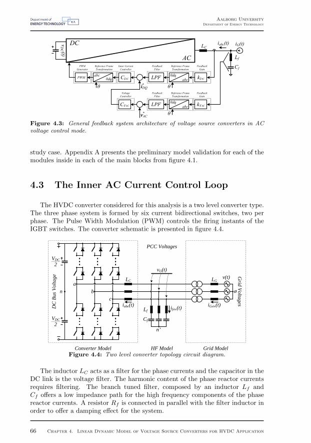
ii
“Thesis” — 2012/11/2 — 9:02 — page 66 — #66 ii
ii
ii
Aalborg UniversityDepartment of Energy Technology
iG(t)vD
C (t)
DC
CIAC
Inner CurrentController
Reference FrameTransformation
abc0dq
Reference FrameTransformation
abc0dqPWM
PWMGenerator
kIAC
FeedbackGain
iDQi*
kVAC
FeedbackGain
LPF
FeedbackFilter
θ θ
iabc(t)
AC
LC
Lf
Cf
LPF
FeedbackFilter
CVAC
VoltageController
v*vAC
Reference FrameTransformation
abc0dq
θ
Figure 4.3: General feedback system architecture of voltage source converters in ACvoltage control mode.
study case. Appendix A presents the preliminary model validation for each of themodules inside in each of the main blocks from figure 4.1.
4.3 The Inner AC Current Control Loop
The HVDC converter considered for this analysis is a two level converter type.The three phase system is formed by six current bidirectional switches, two perphase. The Pulse Width Modulation (PWM) controls the firing instants of theIGBT switches. The converter schematic is presented in figure 4.4.
VDC2
VDC2
n
LCa
bc
v(t)
Lf
Cf
n’
LG
ø
vG(t)
iabc(t) ifabc(t)iGabc(t)
Converter Model HF Model Grid Model
DC
Bus
Vol
tage
PCC Voltages
Grid Voltages
Figure 4.4: Two level converter topology circuit diagram.
The inductor LC acts as a filter for the phase currents and the capacitor in theDC link is the voltage filter. The harmonic content of the phase reactor currentsrequires filtering. The branch tuned filter, composed by an inductor Lf andCf offers a low impedance path for the high frequency components of the phasereactor currents. A resistor Rf is connected in parallel with the filter inductor inorder to offer a damping effect for the system.
66 Chapter 4. Linear Dynamic Model of Voltage Source Converters for HVDC Application

ii
“Thesis” — 2012/11/2 — 9:02 — page 67 — #67 ii
ii
ii
Aalborg UniversityDepartment of Energy Technology
For this study, just one filter branch is included in the system. In real appli-cations, usually, two branches are present; one for the switching frequency andanother branch for twice this frequency.
The power transformer is placed at the output of the converter in order toadapt voltage levels. An equivalent inductor models the effect of the transformerand such inductance is included in the final value of the grid impedance LG. TheAC grid is simplified using an equivalent Thevenin model.
The top level ratings for the system, such as voltage and power levels, werebased in a real system presented in [43] and summarised in table 4.1.
Parameter Value Unit Comment
Power Rating 400 MW [43]
Number of Circuits 1 [43]
AC Voltage 150 kV Assumed
DC Voltage ±150 kV [43]
Converter Type Two-Level VSC
Table 4.1: Parameters for the voltage source converter from reference project [43].
The converter modelling procedure follows the average model; analysis pre-sented by [44, 42]. The converter switching effect is not considered, which meansthat just lower frequencies than the switching frequency can be analysed.
Due to dynamic decoupling, the converter modelling is split in inner and outerloops where the current dynamics is controlled in the inner loop and for the outerloops, the DC or AC voltage compensation are present. The synchronizationbetween grid voltage and converter is performed by the phase-locked loop (PLL)as an extra control loop presented in the system in case of onshore control mode.
In the current loop modelling purpose, the outer loops represented by thevoltage controllers are not considered and the variables related to DC and ACvoltages, as well as the converter current references are taken as inputs for thesystem. The proper model of the figure 4.4 can be split in three main blocks: onerepresenting the current control loop detailed in figure 4.5 and two extra blocksrepresenting the dynamics of the high frequency filter and the grid impedance.Figure 4.5 illustrates the interconnection among the main blocks considered inthe AC current inner loop.
The grid model contains the dynamic properties of the grid impedance set bythe assumed short circuit ratio. The high frequency filter model covers the differ-ential equations relating the filter capacitor, the filter inductor and the dampingresistor connected in parallel with it. The converter model, controller, measuringdevices and modulator are all included in the converter current loop block.
The PLL is the synchronisation loop. It is not explicitly shown in figure 4.4,however, it is represented an external block in the figure 4.5. The phase-lockloop is not present in the offshore converter station controller as well due to thefact that the VSC-HVDC converter imposes the amplitude and frequency for thevoltages at the point of common coupling with the AC collector of the offshore
Chapter 4. Linear Dynamic Model of Voltage Source Converters for HVDC Application 67

ii
“Thesis” — 2012/11/2 — 9:02 — page 68 — #68 ii
ii
ii
Aalborg UniversityDepartment of Energy Technology
vDC(t)
vGDQ(t)
ω
iDQ(t) Con
vert
er
Cur
rent
Loo
p
i*
iDQ(t)vDQ(t)
Gri
dC
urre
nt iGDQ(t) if DQ(t)
vGDQ(t)
HF
Filte
r
PLL
ω
ωt
ωo
ωtωt
ωt
Figure 4.5: Block diagram representation of inner current controller.
wind farm.
For the converter control loop, the most inner loop is the converter model, thefigure 4.6 illustrates the general control block diagram of a VSC.
vG(t)vDC(t)
DC
CIAC
CurrentController
Reference FrameTransformation
abc0dq
Reference FrameTransformation
abc0dqPWM
PWMGenerator
kIAC
FeedbackGain
iDQi*
kVAC
FeedbackGain
LPF
FeedbackFilter
θ θ FeedbackFilter
PLLθ
iabc(t)
AC
LC
Lf
Cf
Figure 4.6: General VSC control block diagram for the current control.
From figure 4.4, vG(t) is the instantaneous grid voltage at the point of com-mon coupling (PCC), LC is the phase reactor inductance, dn(t) is the PWM firingpulse of the nth IGBT, vC(t) is the instantaneous DC voltage at the terminalsof the converter and CDC is the DC link capacitor. m(t) is the continuous mod-ulation index signal applied in the modulator to generate the gate signals. Theinstantaneous grid voltages are cosine waveforms written in (4.1), (4.2) and (4.3).
vGa(t) = VG cos (ωt+ θG) (4.1)
vGb(t) = VG cos
(ωt− 2π
3+ θG
)(4.2)
vGc(t) = VG cos
(ωt+
2π
3+ θG
)(4.3)
Considering the circuit from figure 4.4, from the Kirchhoff’s voltage law, theconverter output voltages at the points a, b and c and the grid voltages vGa(t),vGb
(t) and vGc(t) can be written according to equations (4.4), (4.5) and (4.6).
vGa(t) = Lc
d
dtia(t) + va(t) + vn(t) (4.4)
68 Chapter 4. Linear Dynamic Model of Voltage Source Converters for HVDC Application

ii
“Thesis” — 2012/11/2 — 9:02 — page 69 — #69 ii
ii
ii
Aalborg UniversityDepartment of Energy Technology
vGb(t) = Lc
d
dtib(t) + vb(t) + vn(t) (4.5)
vGc(t) = Lcd
dtic(t) + vc(t) + vn(t) (4.6)
Equations (4.4), (4.5) and (4.6) are in the abc reference frame. For simplifi-cation purpose, the linear transformation given by (4.7) is applied.
A−1 =
√2
3
1 0 00 cos (ωt) sin (ωt)0 − sin (ωt) cos (ωt)
1√2
1√2
1√2
1 −0.5 −0.5
0√
32 −
√3
2
(4.7)
where A−1 represents the transformation matrix from the abc frame (canonicalvector space) to rotating vector space such as is presented, generally, by equa-tion (4.8).
xφdq = A−1xabc (4.8)
where xabc are the coordinates of any three dimensional vector, which can betransformed to the new basis (φdq) by means of the Park’s power invariant trans-formation A−1.
Expanding the variables that represents the output voltage of the voltagesource converter by its relationship representation with DC link voltage and mod-ulation index and considering (4.7), it is possible to derive (4.9), (4.10) and (4.11).
Lcd
dtiø(t) = vGø(t)−mø(t)
vDC(t)
2− vn(t) (4.9)
Lcd
dtiD(t) = vGD
(t)−mα(t)vDC(t)
2+ ωLCiQ(t) (4.10)
Lcd
dtiQ(t) = vGQ
(t)−mβ(t)vDC(t)
2− ωLCiD(t) (4.11)
Rewriting (4.9), (4.10) and (4.11) using vectorial form, and considering thatthe converter is working under balanced three-phase condition, which eliminatesthe necessity to carry the zero sequence component, the final equation for the ACconverter current model is represented by (4.12).
Lcd
dtiDQ(t) = vGDQ
− vDC(t)
2mDQ(t) + ω
[0 1−1 0
]iDQ(t) (4.12)
For the purpose of this thesis, the model does not consider grid unbalanceswhat simplifies (4.12) by considering just the last two components of the vectors(d and q components). The grounding current is also not considered. With thisexamination, (4.12) can be represented by the block diagram from figure 4.7.
Chapter 4. Linear Dynamic Model of Voltage Source Converters for HVDC Application 69

ii
“Thesis” — 2012/11/2 — 9:02 — page 70 — #70 ii
ii
ii
Aalborg UniversityDepartment of Energy Technology
1s
1LC
LC
mDQ(t)
vG(t)
iDQ(t)
ω
iDQ(t)
vDC(t) 0.510
0-1
Figure 4.7: Block diagram of the non-linear model of converter AC current.
4.3.1 Small Signal Linear Model
The model from (4.12) is a non-linear model. The non-linearities are repre-sented by the multiplier blocks from figure 4.7. In order to obtain a linear modelfor the converter current loop, a linearisation process using Taylor’s Series is used.The Taylor’s Series of the multiplication of two time domain variables x(t) andy(t) can be written such as (4.14).
x(t)y(t) ≈ XY + (x(t)−X)∂
∂x(t)(x(t)y(t))
∣∣∣∣X,Y
+
+ (y(t)− Y )∂
∂y(t)(x(t)y(t))
∣∣∣∣X,Y
(4.13)
x(t)y(t) ≈ XY +X∆y(t) + Y∆x(t) (4.14)
where X and Y are the values of the x(t) and y(t) variables at the equilibriumpoints and ∆x(t) and ∆y(t) are the increment variables. The approximation doesnot consider the higher order terms.
The standard form for representing dynamic linear systems is through statespace model, where a n order system has its coupled differential equations repre-sented by a set of first order differential equations and its input-to-output relation-ship are preserved. The standard state space representation is shown by (4.15).
xn×1(t) = An×nxn×1(t) + Bn×pup×1(t)yq×1(t) = Cq×nxn×1(t) + Dq9×pup×1(t)
(4.15)
where x are the n state variables, u and y the p input and q output signals respec-tively. The general block diagram for the state model from (4.14) is illustrated inthe figure 4.8.
The complete model of the AC side of the voltage source converter is split infour sub-systems with connection diagram presented in figure 4.5. The completestate space model for the AC currents and AC voltages for such device is dividedin the following tasks:
• Converter modelling
– AC current (iabc(t))
70 Chapter 4. Linear Dynamic Model of Voltage Source Converters for HVDC Application

ii
“Thesis” — 2012/11/2 — 9:02 — page 71 — #71 ii
ii
ii
Aalborg UniversityDepartment of Energy Technology
1s
A
B C
D
u(t) y(t)x(t)x(t)
Figure 4.8: State space representation system block diagram.
– AC current controller
– Feedforward compensation
• Grid current modelling (iGabc(t))
• High frequency filter modelling (ifabc(t) and vGabc(t))
• Synchronisation (PLL) modelling
4.3.1.1 Converter Current State Space Model
Linearising (4.12) by means of (4.14), the linear model for the AC currents ofthe voltage source converter can be represented by the linear state space modelin (4.15). Its linearised block diagram is illustrated in figure 4.9.
1s
1LC
LC
ΔmDQ(t)
vG(t)
ΔiDQ(t)
Δω
ΔiDQ(t)
ΔvDC(t) MDQ
VDC0.5
0.5
IDQ
ω
10
0-1
Figure 4.9: Block diagram of the linear model of converter AC current.
The non-linearity given by the multiplier block is replaced by a summationand gains which values are referenced by the system operating points.
The state space realization for the current loop considers as inputs the modu-lation signals ∆mDQ, DC and AC voltages ∆vDC and ∆vGDQ
, and grid frequency∆ω. The state variables are the converter AC currents in the synchronous refer-ence frame multiplied by the phase reactor inductance ∆iDQ. The state vector,
Chapter 4. Linear Dynamic Model of Voltage Source Converters for HVDC Application 71

ii
“Thesis” — 2012/11/2 — 9:02 — page 72 — #72 ii
ii
ii
Aalborg UniversityDepartment of Energy Technology
input and output vectors are given by (4.16), (4.17) and (4.18), respectively.
xP (t) =[LC∆iD(t) LC∆iQ(t)
]T(4.16)
uP (t) =[
∆vDC(t) ∆vGD(t) ∆vGQ
(t) ∆ω
∆mD(t) ∆mQ(t)]T
(4.17)
yP (t) =[
∆iD(t) ∆iQ(t)]T
(4.18)
The state space matrices, AP , BP , CP and DP , for the current loop is givenby (4.19), (4.20), (4.21) and (4.22).
AP =
[0 ω−ω 0
](4.19)
BP =
[ −MD
2 1 0 IQLC −VDC
2 0
−MQ
2 0 1 −IDLC 0 −VDC
2
](4.20)
CP =
[ 1LC
0
0 1LC
](4.21)
DP =
[0 0 0 0 0 00 0 0 0 0 0
](4.22)
The converter parameters are calculated according to the general project de-scription give by [43]. The main values related to the block diagram from figure 4.9are presented in table 4.2.
Parameter Value Unit Comment
Nominal Converter Power 400 MVA [43]
DC Link Voltage ±150 kV [43]
AC Voltage 150 kV Assumed
Phase Reactor 21.5 mH 0.12pu - Assumed
Converter Topology Two level
Switching Frequency 1950 Hz Assumed
Modulation Type Carrier-triangular-based PWM
Table 4.2: Parameters for the voltage source converter.
4.3.1.2 Proportional-Integral Control Action
The traditional controller adopted to compensate the error in the currentclosed loop system is a proportional-integral (PI) compensator type. The pro-portional part improves the system response and, meanwhile, the integral actionguarantees zero error at steady state. The block diagram of a proportional-integralcontroller is presented by figure 4.10.
From figure 4.10, the reference signal r(t) is compared with the measuredsystem output signal y′(t) and a error e(t) is generated. This signal is processed
72 Chapter 4. Linear Dynamic Model of Voltage Source Converters for HVDC Application

ii
“Thesis” — 2012/11/2 — 9:02 — page 73 — #73 ii
ii
ii
Aalborg UniversityDepartment of Energy Technology
1s
kP
ProportionalGain
kI
IntegralGain
r(t)
y’(t)
u(t)
Figure 4.10: General block diagram of a proportional-integral compensator.
by the proportional and integral branches and combined to the controller outputsignal u(t) which will drive the plant to the proper changes based in the errorsignal condition.
The states are the integrator input signals from 4.10. Two states are requiredsince the vector control is adopted and they are labelled xII and xIQ . The inputsare the reference signals i∗D and i∗Q and the feedback output signals i′D and i′Q.The PI output signals are uD and uQ.
For the current loop, where both, direct and quadrature, components of thecurrents are controlled, the state space model for its PI compensator is givenby (4.23) and (4.24), where kI and kP are the proportional and integral gainstuned for a desired dynamic response.
[˙xII (t)˙xIQ(t)
]=
[0 00 0
] [xII (t)xIQ(t)
]+ . . .
[−kID kID 0 0
0 0 −kID kID
]
i∗D(t)i′D(t)i∗Q(t)
i′Q(t)
(4.23)
[uD(t)uQ(t)
]=
[1 00 1
] [xII (t)xIQ(t)
]+ . . .
[−kPD
kPD0 0
0 0 −kPDkPD
]
i∗D(t)i′D(t)i∗Q(t)
i′Q(t)
(4.24)
Combining the state space model for the PI controller and the previous equa-tions which describes the dynamics for the current loop and the feedback filter,the closed loop system for the current control of the voltage source converter isachieved. The parameter used for the current controller are given by the table 4.3.
4.3.2 Disturbances Effect
The control strategy adopted is a feedback control with PI controller. Theintegral gain guarantees the zero error in steady-state and the proportional gain
Chapter 4. Linear Dynamic Model of Voltage Source Converters for HVDC Application 73

ii
“Thesis” — 2012/11/2 — 9:02 — page 74 — #74 ii
ii
ii
Aalborg UniversityDepartment of Energy Technology
Parameter Value Unit
Proportional Gain 1.0
Integral Gain 2450
Bandwidth 390 Hz
Table 4.3: AC current PI controller parameters.
improves the dynamic response. More than just the control inputs, the feedfor-ward terms are presented in order to assist faster response for the measurabledisturbances: DC link voltage, grid voltage and coupling effect.
4.3.2.1 Feedback Linearization for DC Bus Voltage
The DC link voltage variation has effect over the output currents. The effectis directly compensated in the controller and the control commands mitigates,under a transient response, the consequence. The feedforward for the voltagecontroller is also included in the EMTDC and small signal model as illustrated infigure 4.11.
mDQ(t)
vDC(t)
0.5Feedback Gain
kVDC
Feedforward Gain
kVDCkFF
Feedback Linearization1s
1LC
LC
vG(t)
iDQ(t)
ω
iDQ(t)
10
0-1
Figure 4.11: Feedback linearization by means of feedforward control of DC link voltage.
The feedforward path for the DC link voltage directly influences the controller,since all the effort for DC link disturbance mitigation is driven by the DC feed-forward controller.
4.3.2.2 Grid Voltages Feedforward
From the dynamic model presented in the figure 4.8 shows the voltage at thepoint of common coupling as a disturbance input. This reflects in the controlaction during voltage transients, since the AC voltages have the additive effect.
In the presence of the feedforward control action, the effect of the voltagedisturbances is mitigated on the current response. The feedforward for the AC
74 Chapter 4. Linear Dynamic Model of Voltage Source Converters for HVDC Application

ii
“Thesis” — 2012/11/2 — 9:02 — page 75 — #75 ii
ii
ii
Aalborg UniversityDepartment of Energy Technology
voltage compensation is represented by a simple signal addition in the outputof the current control. Just the sensor gain and a feedforward gain kFFiAC
arerequired to scale properly the signal in the control level. The error signals are notnoticeably influenced by such variation. As a consequence, the control signal fromthe feedforward direct compensation takes the lead for disturbance reduction.
4.3.2.3 Feedback Linearisation for Decoupling Network
The effect of the current coupling terms in the synchronous reference frameappear where changes in each of the axis current references reflects in distur-bances in the opposite current component. A feedforward term can be includedin the complete control model, that such compensation is directly performed by asecondary branch in loop. As a consequence, the influence of one component intoanother is attenuated and the PI control does not have action in such situation.
4.3.2.4 Structure of the Inner Current Controller Feedforward
The disturbances presented in the current loop can distort the converter outputcurrents and, as a consequence, the current controller is required to act to mitigatesuch effect. For fast response, however, the feedforward terms are included.
For the DC link voltage and the coupling between the DQ-axes currents,the feedforward requires non-linear operations. For the AC grid voltages, thecompensation is made by a linear combination os signals.
Considering the the whole current controller as a combination of the PI con-troller, DC voltage, AC voltage and decoupling feedforward terms, the blockdiagram of the of the complete inner loop compensator is depicted in figure 4.12.
kFF
Δi’DQ(t)
Δω
1s
uDQP(t)
uDQI(t)
v’G(t)
ΔmDQ(t)
LC
Δv’DC(t)
10
0-1
kVDCkFF
kIAC
uPIDQ(t)
Figure 4.12: Current controller block diagram with PI and feedforward compensation.
where the ′ symbols are the input variables weighted by the sensor gains. The
Chapter 4. Linear Dynamic Model of Voltage Source Converters for HVDC Application 75

ii
“Thesis” — 2012/11/2 — 9:02 — page 76 — #76 ii
ii
ii
Aalborg UniversityDepartment of Energy Technology
input and output vectors a given by (4.25) and (4.26), respectively.
uPI(t) =[v′DC(t) v′GD
(t) v′GQ(t) ω i′D(t) i′Q(t) . . .
uPID (t) uPIQ(t)]
(4.25)
yPI(t) =[mD(t) mQ(t)
]T(4.26)
The algebraic matrix which relates the output of the complete control model∆mDQ(t) and the PI output uPIDQ
(t) including the feedforward linearised com-pensation are presented in equation (4.27).
PIFF =
[ −MD
V ′′ 2DC
1V ′′DC
0IQLC
V ′′DC
0 ωLC
V ′′DC
1V ′′DC
0−MQ
V ′′ 2DC
0 1V ′′DC
−IDLC
V ′′DC
−ωLC
V ′′DC
0 0 1V ′′DC
]
(4.27)
The double prime symbols in the parameters in (4.27) are referenced to themeasured input variables weighted by the feedforward gains in figure 4.12.
4.4 Grid Synchronisation
A phase locked loop (PLL) is required in the connection of voltage sourceconverters and electric grid for the propose of reference tracking. The generationof unit sine and cosines signals required in the reference frame transformation isbasically originated by the synchronization block. By then, it is required for thePLL an accurate tracking of the grid angle even under abnormal grid operationand under some harmonic content conditions [42, 45].
The basic structure of the three-phase synchronously rotating reference frame(SRF) based PLL has the basic block diagram illustrated by the figure 4.13.
vGa(t)
vGb(t)
vGc(t)
ReferenceFrame
TransformationPI(s)
PIController
ωo
OSC
Oscilator Block
PhaseDetector
vα(t)
vβ(t)
Figure 4.13: Simplified block diagram of SFR PLL.
The phase detector is responsible for generating the output signal proportionalto the phase difference between the grid angle and generated angle reference. Theloop filter, a PI controller which leads the error difference to zero in steady state.The voltage oscillator block generates the output signal whose frequency is afunction of the input frequency of the grid.
Considering that the grid angle is represented by θ, as well as a balancedgrid condition, the α and β components for the rotating frame is given by (4.28)
76 Chapter 4. Linear Dynamic Model of Voltage Source Converters for HVDC Application

ii
“Thesis” — 2012/11/2 — 9:02 — page 77 — #77 ii
ii
ii
Aalborg UniversityDepartment of Energy Technology
and (4.29).
v′
α(t) =
√3
2V
′
G cos (θ) (4.28)
v′
β(t) =
√3
2V
′
G sin (θ) (4.29)
The output of the multiplicative phase detector from figure 4.13 extracts thephase of the system by means of 4.30.
√3
2V
′
G sin (θ − ωt) = −√
3
2V
′
G cos (θ) sin (ωt) . . .
+
√3
2V
′
G sin (θ) cos (ωt) (4.30)
For small angle differences the component sin (θ − ωt) gives approximatelythe value of difference between the grid angle and the PLL synchronizing currentangle. Considering the simplification from 4.30, the non-linear block diagram fromfigure 4.13 can be simplified by the linearised PLL control architecture given bythe figure 4.14.
PI(s)
PIController
ωo
OSC
Oscilator Block
PhaseDetector
VGV’ ωωt
θ
Figure 4.14: Linearised block diagram for the SRF PLL.
The state space representation of the system in which the block diagram isdepicted in figure 4.14 is characterised by the matrices APLL, BPLL, CPLL andDPLL. The input signals are the angle θ of the voltage at the PCC and nominalvalue of the grid angular frequency ωo. The output of the PLL state space modelis the PLL angle ωt. The states are the integrators from the PI integrator andfrom the voltage oscillator, respectively. The state space representation is by then,given through the equations (4.31) and (4.32).
[xPLLPI
(t)xPLLOSC
(t)
]= APLL
[xPLLPI
(t)xPLLOSC
]+BPLL
[θωo
](4.31)
ωt = CPLL
[xPLLPI
(t)xPLLOSC
]+DPLL
[θωo
](4.32)
By then, the state space representation of the grid synchronisation block is
Chapter 4. Linear Dynamic Model of Voltage Source Converters for HVDC Application 77

ii
“Thesis” — 2012/11/2 — 9:02 — page 78 — #78 ii
ii
ii
Aalborg UniversityDepartment of Energy Technology
explicitly showed by (4.33), (4.34), (4.35) and (4.36).
APLL =
[0 −V ′GkIPLL
−1 V ′GkPPLL
](4.33)
BPLL =
[V ′GkIPLL
0−V ′GkPPLL
1
](4.34)
CPLL =[
0 1]
(4.35)
DPLL =[
0 0]
(4.36)
The parameter V ′G represents the weighted amplitude of the voltage at thepoint of common coupling and kIPLL
and kPPLLthe parameters of the PI com-
pensator. The control parameters for the nominal operating points are presentedin table 4.4.
Parameter Value Unit
Proportional Gain 92
Integral Gain 628.3185
Table 4.4: Control parameters for the PLL synchronisation loop.
4.5 Grid Impedance and High Frequency FilterModels
The grid impedance can play an important role in the integration of the con-verter and the grid. For stiff grids, the impedance has a small effect under theeffect of the other modes presented by internal converter loops. When the grid isconsidered a weak grid, this impedance may have effect over the other controllersand the performance of the entire system can unexpectedly be lower than the onein which it was design for[46]. The differential equation for the grid impedanceconsidering the model presented by 4.4 is written by (4.37).
v(t) = LGdiG(t)
dt+RGiG(t) + vG(t) + v
′
n(t)
111
(4.37)
where, v(t) is the internal grid voltage vector, LG the equivalent grid inductanceand RG is the equivalent grid series resistance. iG(t) represents the convertercurrents after the high frequency filtering effect.
In equation (4.37) is written in the abc frame. The transformation from (4.7)is still valid and can remove the effect of the zero sequence for balanced grid con-ditions. Equation (4.37) can be written in synchronous reference frame according
78 Chapter 4. Linear Dynamic Model of Voltage Source Converters for HVDC Application

ii
“Thesis” — 2012/11/2 — 9:02 — page 79 — #79 ii
ii
ii
Aalborg UniversityDepartment of Energy Technology
to (4.38).
LGdiGDQ
(t)
dt+RGiGDQ
(t) = vDQ(t)− vGDQ(t) + . . .
ωLG
[0 1−1 0
]iGDQ
(t) (4.38)
For the equation (4.38), the block diagram for such differential equation isrepresented by figure 4.15.
1s
1LG
ω
iDQG(t)
10
0-1 LG
RG
vG(t)
v(t)
LG
Figure 4.15: Block diagram for the grid current dynamic model.
The state, input and output vector from the model in the figure 4.15 are givenin (4.39), (4.40) and (4.41).
xG(t) =[LGiGD
(t) LGiGQ(t)
]T(4.39)
uG(t) =[v(t) vG(t) ω
]T(4.40)
yG(t) =[iGD
(t) iGQ(t)
]T(4.41)
The state space matrices for the grid impedance linear model are given bythe (4.42), (4.43), (4.44) and (4.45).
AG =
[−RG
LGω
−ω −RG
LG
](4.42)
BG =
[1 0 −1 0 LGIQG
0 1 0 −1 −LGIDG
](4.43)
CG =
[ 1LG
0
0 1LG
](4.44)
DG =
[0 0 0 0 00 0 0 0 0
](4.45)
Chapter 4. Linear Dynamic Model of Voltage Source Converters for HVDC Application 79

ii
“Thesis” — 2012/11/2 — 9:02 — page 80 — #80 ii
ii
ii
Aalborg UniversityDepartment of Energy Technology
The high frequency filter included in the circuit for current filtering is a shuntsecond order filter [47]. It acts as single-tuned filter for frequency below theresonance frequency, and as a high pass filter at higher the resonance. From thefigure 4.4, the circuit of the high frequency filter is simplified. The schematic ofthis branch filter is illustrated in figure 4.16.
Lf
Cf
n’
ifabc(t)
vG(t)
Cf
n’
vG(t)
vC f (t)
Lf i Lf (t
)
Rf
ifabc(t)
Figure 4.16: Shunt second order passive filter.
For the high frequency filter, the differential equation which relates the filtercurrents if (t) and the voltage at the point of common coupling with the voltagesource converter vG(t) is given by (4.46).
CfLfRf
d2vG(t)
dt2+ Cf
dvG(t)
dt= CfLf
d2if (t)
dt2+LfRf
dif (t)
dt+ if (t) (4.46)
where, Cf , Lf and Rf are the filter passive component parameters. if (t) andvG(t), the current and voltages of the high frequency filter, respectively.
Considering the differential equation from (4.46), the block diagram whichrepresents the dynamic property between the input current of the filter and itsvoltage is given by figure 4.17.
1s
1s
Δifabc(t)
ΔvGabc(t)Cf Lf
Rf
Rf
Lf
Cf LfLf
Rf
Figure 4.17: Block diagram for the high frequency filter dynamic model.
In the synchronous reference frame, considering the previous transformationpresented by (4.7), the vectorial form for the high frequency filter differential
80 Chapter 4. Linear Dynamic Model of Voltage Source Converters for HVDC Application

ii
“Thesis” — 2012/11/2 — 9:02 — page 81 — #81 ii
ii
ii
Aalborg UniversityDepartment of Energy Technology
equation is give in (4.47).
CfLfRf
d2vGDQ(t)
dt2+ Cf
dvGDQ(t)
dt= CfLf
d2ifDQ(t)
dt2+LfRf
difDQ(t)
dt+ . . .
ifDQ(t) + ω2CfLf
RfvGDQ
(t) + . . .
ωCf
[0 1−1 0
]vGDQ
(t)− . . .
ω2CfLf ifDQ(t)− . . .
ωCfLf
[0 1−1 0
]ifDQ
(t) (4.47)
For the state variables given byLf
RfiLf
and its derivative, the matrices of the
linearised state space model for the HF filter is represented by (4.48), (4.49), (4.50)and (4.51).
AHF =
0 1 ω 0
0 −Rf
Lf0 ω
−ω 0 0 1
0 −ω 0 −Rf
Lf
(4.48)
BHF =
0 0VRfQ
Rf
1 0Lf IRfQ
Rf
0 0 −VRfD
Rf
0 1 −Lf IRfD
Rf
(4.49)
CHF =
Rf
CfLf
1Cf− R2
f
Lf0 0
0 0Rf
CfLf
1Cf− R2
f
Lf
(4.50)
DHF =
[Rf 0 00 Rf 0
](4.51)
The node equation for the currents in the point of common coupling is writtenby (4.52).
iG(t) = if (t) + i(t) (4.52)
The components of the branch tuned filter from figure 4.16 are based in thespecification of reactive power consumption, quality factor and filtering frequency.The specification of the high frequency filter and its parameters are presented intable 4.5. The impedance characteristic of such device is presented in figure 4.18.
Chapter 4. Linear Dynamic Model of Voltage Source Converters for HVDC Application 81

ii
“Thesis” — 2012/11/2 — 9:02 — page 82 — #82 ii
ii
ii
Aalborg UniversityDepartment of Energy Technology
Parameter Value Unit
Reactive Power 26.7 MVA
Quality Factor 25
Notch Frequancy 1950 Hz
Inductance 1.9 mH
Capacitance 3.4 µF
Resistance 600 Ω
Table 4.5: High frequency filter settings.10
110
210
310
410
5−20
0
20
40
60
80
Frequency [Hz]
Magnitude[dB]
Nominal F requency
Switching Frequency
Figure 4.18: Impedance characteristic.
4.6 The Outer DC Voltage Control Loop
The direct DC voltage control method applied in the voltage source converteris able to, indirectly, regulate the power transfer between the AC and DC sides ofthe converter. Using the vector current control, the DC voltage loop is cascadedconnected to the current control, promoting the D-axis reference current for theinner control loop. Changing the amplitude of the reference i∗D current, the activepower transfer is changed. Figure 4.19 brings the representation of the power flowin the two-level converter adopted to the analysis.
vDC(t)2
n
LCa
bc
vG(t)
iabc(t)
pAC(t)
pDC(t)
vDC(t)2
po(t)
Power DeliveredTo DC Link
pC(t)
Figure 4.19: Circuit schematic for voltage source converters with active power flowrepresentation.
From figure 4.19 the input power pAC is processed by the converter resultingin the DC converter power pDC and the converter losses PLosses which is notspecified in the figure. The total power delivered to the DC grid po is a result of
82 Chapter 4. Linear Dynamic Model of Voltage Source Converters for HVDC Application

ii
“Thesis” — 2012/11/2 — 9:02 — page 83 — #83 ii
ii
ii
Aalborg UniversityDepartment of Energy Technology
this DC power subtracted by the power used to charge or discharge the DC linkcapacitors.
The DC voltage control is, then, based in the instantaneous average model,which can be indirectly related with the instantaneous measurement of power inAC systems given by [44], where the active power is defined as the scalar productof the voltage and current vectors according to (4.53).
p(t) :=
(vDC(t)
2uDQ(t)
)· iDQ(t) (4.53)
where iDQ is the current vector which flows through the phase reactors LC , insynchronous reference frame. The term vDC
2 uDQ represents the instantaneousvoltage vector at the point abc from figure 4.19. vDC is the DC bus voltage anduDQ are the modulation indexes.
By applying the energy balanced law in the DC side of the converter from fig-ure 4.19, the instantaneous input energy EDC is numerically equal to the chargingenergy in the DC link capacitor CDC and the output energy delivered to the DClink. This means that the energy balance equation is written according to (4.54).
EDC(t) = EC(t) + Eo(t) (4.54)
Differentiating (4.54) on both sides, it is possible to write the power balancedequation for the two-level converter type according to (4.55).
pDC(t) =d (EC(t))
dt+ po(t) (4.55)
where the voltage versus energy relationship for the capacitor CDC can be writtenaccording to (4.56).
EC(t) =1
2CDCv
2DC(t) (4.56)
Combining (4.56) into (4.55), the dynamic differential equation which de-scribes the properties in the DC link voltage is derived by (4.57).
pDC(t) =1
2CDC
dv2DC(t)
dt+ po(t) (4.57)
Considering the converter control loop from the figure 4.6, the aggregatedinput/output dynamic system can be represented with input signals given by theDC voltage vDC(t), voltage at the point of common coupling vGDQ
, grid frequencyω and referenced for the AC currents in the synchronous reference frame i∗DQ. Theoutput of the current loop is the AC current vector iDQ. The grid angle is alsorequired for the linear transformation presented by (4.7). For such modellingsimplification and making use of equation (4.53), the plant for the DC voltageloop can be illustrated in the block diagram from figure 4.20.
Chapter 4. Linear Dynamic Model of Voltage Source Converters for HVDC Application 83
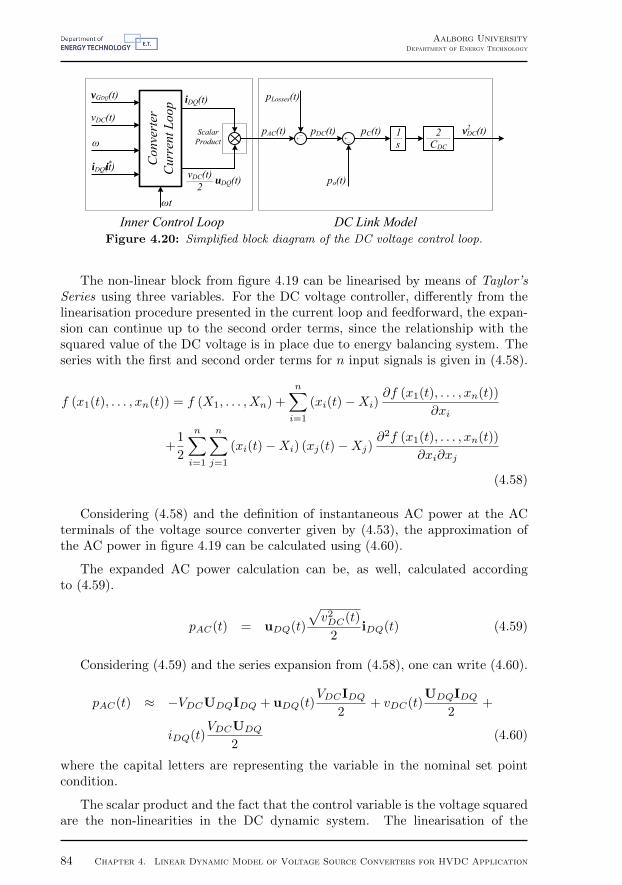
ii
“Thesis” — 2012/11/2 — 9:02 — page 84 — #84 ii
ii
ii
Aalborg UniversityDepartment of Energy Technology
ω
iDQ(t)
Inner Control Loop
i*
iDQ(t)
ωt
vDC(t)
vGDQ(t)
ScalarProduct
pAC(t)
Con
vert
er
Cur
rent
Loo
p
pLosses(t)
pDC(t)
po(t)
pC(t) 1s
2CDC
vDC(t)v2
DC Link Model
vDC(t)2 uDQ(t)
Figure 4.20: Simplified block diagram of the DC voltage control loop.
The non-linear block from figure 4.19 can be linearised by means of Taylor’sSeries using three variables. For the DC voltage controller, differently from thelinearisation procedure presented in the current loop and feedforward, the expan-sion can continue up to the second order terms, since the relationship with thesquared value of the DC voltage is in place due to energy balancing system. Theseries with the first and second order terms for n input signals is given in (4.58).
f (x1(t), . . . , xn(t)) = f (X1, . . . , Xn) +
n∑
i=1
(xi(t)−Xi)∂f (x1(t), . . . , xn(t))
∂xi
+1
2
n∑
i=1
n∑
j=1
(xi(t)−Xi) (xj(t)−Xj)∂2f (x1(t), . . . , xn(t))
∂xi∂xj
(4.58)
Considering (4.58) and the definition of instantaneous AC power at the ACterminals of the voltage source converter given by (4.53), the approximation ofthe AC power in figure 4.19 can be calculated using (4.60).
The expanded AC power calculation can be, as well, calculated accordingto (4.59).
pAC(t) = uDQ(t)
√v2DC(t)
2iDQ(t) (4.59)
Considering (4.59) and the series expansion from (4.58), one can write (4.60).
pAC(t) ≈ −VDCUDQIDQ + uDQ(t)VDCIDQ
2+ vDC(t)
UDQIDQ2
+
iDQ(t)VDCUDQ
2(4.60)
where the capital letters are representing the variable in the nominal set pointcondition.
The scalar product and the fact that the control variable is the voltage squaredare the non-linearities in the DC dynamic system. The linearisation of the
84 Chapter 4. Linear Dynamic Model of Voltage Source Converters for HVDC Application

ii
“Thesis” — 2012/11/2 — 9:02 — page 85 — #85 ii
ii
ii
Aalborg UniversityDepartment of Energy Technology
dynamic system follows the procedure presented in (4.60) and the linear statespace model has state variable and input/output signals given by (4.61), (4.62)and (4.63).
xDC(t) =
[CDC
2v2DC(t)
](4.61)
uDC(t) =[po(t) vDC(t) iDQ(t) uDQ(t)
]T(4.62)
yDC(t) =[v2DC(t) vDC(t)
]T(4.63)
It is necessary to mention that the converter losses are going to be treatedas a non-modelled variable and its effect is not considered in the linear model.Another issue related with the model from figure 4.20 is the output vector yDC .In the small signal model the control variable is given by the square of the DClink voltage. However, the value of vDC is required for the completeness of theoverall model.
The matrices from the linear state model for the DC voltage plant are repre-sented by the equations written in
ADC =[
0]
(4.64)
BDC =[−1
UDQIDQ
2VDCUDQ
2VDCIDQ
2
](4.65)
CDC =
[ 2CDC
1CDCVDC
](4.66)
DDC =
[0 0 0 0 00 0 0 0 0
](4.67)
4.7 The Outer AC Voltage Control Loop
For wind applications, the HVDC converter station at the offshore side isresponsible for sustain the AC voltage at the point off common coupling. Forthat reason the AC voltage control mode is activated. For this mode of operationthe control block diagram from figure 4.3 is enabled.
In the AC voltage control mode, the PLL is not present and the two, voltagemagnitude and its angle, are directly imposed by the HVDC converter in the PCCnode. This control mode emulates an infinite bus viewed from the wind farms.
In this work, the offshore wind farms are modelled as current sources were itsamplitude is proportional to the wind power. With this simplification of the windpower plants, the representation of the voltage source converter connected to theweak offshore grid as shown in the figure 4.21.
Figure 4.5, previously presented, illustrates basically a simplification of theAC system for the onshore converter control mode. In the onshore, due to the
Chapter 4. Linear Dynamic Model of Voltage Source Converters for HVDC Application 85

ii
“Thesis” — 2012/11/2 — 9:02 — page 86 — #86 ii
ii
ii
Aalborg UniversityDepartment of Energy Technology
VDC2
VDC2
n
LCa
bc
Lf
Cf
n’
ø
vG(t)
iabc(t) ifabc(t)
iGabc(t)
Converter Model HF Model Grid Model
DC
Bus
Vol
tage
PCC Voltages
Wind FarmModel
Figure 4.21: Representation of the circuit diagram of the offshore voltage source con-verter station.
emulation of an ideal voltage at the point of common coupling, some of the blocksare, consequently, removed. They are the PLL and the grid model.
The synchronisation for the voltage source converter is not allowed at the off-shore station. The wind turbines have internally the ability to keep synchronisedto the HVDC station and the angle is directly imposed. The grid was simplifiedby a pure current source with amplitude value proportional the amount of powerproduced by the wind power plant. Considering the mentioned simplification, theblock diagram representing the main system from the offshore side is illustratedin the figure 4.22.
vDC(t)
vGDQ(t)
ω
iDQ(t) Con
vert
er
Cur
rent
Loo
p
i*
iDQ(t)
pWPP(t)Current
CalculationiGDQ(t) if DQ(t)
HF
Filte
r
ωt ωt
ωt
qWPP(t)
Figure 4.22: Block diagram representation of AC converter side at offshore HVDCstation.
The current calculation block diagram representation from figure 4.22 is analgebraic loop where the input variables are the active and reactive power fromthe wind power plant (pWPP ,qWPP ). The output representing the current vectoriGDQ
, in synchronous reference frame, calculated by (4.68) [44].
[iGD
(t)iGQ
(t)
]=
1
v2GD
(t) + v2GQ
(t)
[vGD
(t) −vGQ(t)
vGQ(t) vGD
(t)
] [pWPP (t)qWPP (t)
](4.68)
86 Chapter 4. Linear Dynamic Model of Voltage Source Converters for HVDC Application

ii
“Thesis” — 2012/11/2 — 9:02 — page 87 — #87 ii
ii
ii
Aalborg UniversityDepartment of Energy Technology
The equation from (4.68) represents a non-linearity in the block diagramfrom 4.22. Four variables represent the input vector of the system. They arethe voltages in the synchronous reference frame, more two components for theactive and reactive powers. The currents, in the linearised form, represent theoutput vector. Differently from the previous series expansion in two dimensional,the calculation of the linearised form of (4.68).
Its linearisation form is represented by (4.69) and the combination with thehigh frequency filter state space model (equations (4.48), (4.49), (4.50) and (4.51))and the inner current loop form the offshore VSC-HVDC station dynamic model.
[iGD
(t)iGQ
(t)
]=
1(V 2GD
+ V 2GQ
)2 M
vGD(t)
vGQ(t)
pWPP (t)qWPP (t)
(4.69)
where M is the matrix with the elements given by (4.70).
M11 = −(V 2GD− V 2
GQ
)PWPP + 2V 2
GDVGQQWPP
M12 = −(V 2GD− V 2
GQ
)QWPP − 2V 2
GDVGQPWPP
M13 = VGD
(V 2GD
+ V 2GQ
)
M14 = − VGQ
(V 2GQ
+ V 2GQ
)
M21 = −(V 2GD− V 2
GQ
)QWPP − 2V 2
GDVGQPWPP
M22 =(V 2GD− V 2
GQ
)PWPP − 2V 2
GDVGQQWPP
M23 = VGQ
(V 2GD
+ V 2GQ
)
M24 = VGD
(V 2GQ
+ V 2GQ
)
(4.70)
The combination of the equation (4.69) and the state model for the currentcontrol as well as for the high frequency filter defines the state space model forthe offshore converter station. The inner current controller for this station hasthe same settings as the ones presented by the converter in which the DC voltagecontrol mode was applied. Due to the weakness of the offshore grid, the highfrequency filter parameters were changed. The increase in the reactive power andthe decrease in the quality factor were adjusted by simulations. The parametersfor the high frequency filter for the offshore converter station is presented intable 4.6 and its impedance characteristic is given in the figure 4.23.
For the PI control parameters the table 4.7 contains the settings for the tunedvalues of the AC voltage control loop.
4.8 VSC-HVDC Transmission Dynamic Model
The modelling process presented above was designed by spiting a larger sys-tem, represented by the voltage source converter plant and its controllers, in smallpieces in which the block diagrams from figures 4.2 and 4.3 show in details the
Chapter 4. Linear Dynamic Model of Voltage Source Converters for HVDC Application 87

ii
“Thesis” — 2012/11/2 — 9:02 — page 88 — #88 ii
ii
ii
Aalborg UniversityDepartment of Energy Technology
Parameter Value Unit
Reactive Power 68.9 MVA
Quality Factor 5
Notch Frequancy 1950 Hz
Inductance 784.7 µH
Capacitance 8.4 µF
Resistance 48.1 Ω
Table 4.6: High frequency filter settings.10
110
210
310
410
5−20
0
20
40
60
80
Frequency [Hz]
Magnitude[dB]
Nominal F requency
Switching Frequency
Figure 4.23: Impedance characteristic.
Parameter Value Unit
Proportional Gain 1.0
Integral Gain 490.1
Bandwidth 78 Hz
Table 4.7: AC voltage PI controller parameters.
smaller pieces. For a single-link VSC-HVDC transmission, the top level buildingblocks of the system are:
• Wind power plant
• Offshore AC cabling
• Offshore HVDC converter
• DC Cabling
• Onshore HVDC converter
• Grid
Grouping all the main systems itemized above, the six modules are able todescribe a single-link VSC-HVDC transmission from a offshore wind park to shoreby means of grid connected voltage source converter and are systematised infigure 4.1
From the modelling process performed in the previous sections in this chap-ter, the wind power plant was simplified using only current sources, where theamplitude of the current is directly proportional to the power delivered by thewind energy. The angle is defined by the offshore HVDC station. The modellingof the mechanical and electrical parts as well as the layout of a wind energy is notpresented and focused in this work. Using this level of simplification, the windfarm and the AC cables are represented by the algebraic equation relating theelectrical variables in the point of common coupling from (4.69). The AC cablebetween the AC collector of the wind power plant and the HVDC converter is notmodelled.
88 Chapter 4. Linear Dynamic Model of Voltage Source Converters for HVDC Application

ii
“Thesis” — 2012/11/2 — 9:02 — page 89 — #89 ii
ii
ii
Aalborg UniversityDepartment of Energy Technology
The converter models were presented in the above sections. Both controlmodes are operative for a single link HVDC transmission. At the offshore side,the AC voltage control mode is active. With this operation mode, the offshoreAC collection point is emulated such as an infinite bus for the wind turbines. Forthe onshore station, the DC voltage controller is activated. By this means, theDC voltage is kept constant in steady state and during transients, the controlcompensates the disturbance actions. The simple grid model is used for thissystem as well as the synchronisation method presented in the previous sections.
4.8.1 DC Cable Simplified Dynamic Model
The representation of the cable in the VSC-HVDC transmission present infigure 4.1 includes the DC submarine cables. This due to the consideration thatthe benchmark system is developed for offshore application. The cable modelling,however, can assume from simple modelling process (π-section approximation) toBergeron and frequency dependent models.
The representation of the cable using π-section considers the connection ofN modules characterized by two capacitors, one inductor and one resistor torepresent the losses. The circuit diagram representation of a cable π-section isshowed by figure 4.24 [48].
Cs2
iOff (t) RsLs iOn(t)
Cs2vOff (t) vOn (t)
Figure 4.24: Circuit diagram for a single π-section for cable modelling.
Taking into account the representation of the π-section from figure 4.24, themathematical model for such circuit can be represented by a third order differen-tial equation. Defining the system states as the voltages at the shunt capacitorsand the current in the series inductor and system inputs as the offshore and on-shore DC currents, the dynamic representation of one π-section by means of statespace approach is given by the equations (4.71) and (4.72).
vOff (t)vOn(t)
iLs(t)
=
0 0 −2Cs
0 0 −2Cs
1Ls
−1Ls
−1Ls
vOff (t)vOn(t)iLs
(t)
+
1 00 10 0
[iOff (t)iOn(t)
](4.71)
vOff (t)vOn(t)iLs
(t)
=
1 0 00 1 10 0 0
vOff (t)vOn(t)iLs
(t)
+
0 00 00 0
[iOff (t)iOn(t)
](4.72)
By the cascade connection of N π-sections in the system, the HVDC simplifiedcable model can be represented by the schematic circuit from figure 4.25.
Chapter 4. Linear Dynamic Model of Voltage Source Converters for HVDC Application 89

ii
“Thesis” — 2012/11/2 — 9:02 — page 90 — #90 ii
ii
ii
Aalborg UniversityDepartment of Energy Technology
CDCCs2
iOff (t) RsLs
Cs2
N -2 Sections Cs2
RsLs iOn(t)
Cs2
Rs
CDC
Rs
Figure 4.25: Schematic representation of DC cable interconnection using π-sections.
For the system representation illustrated by the figure 4.1, the parameters re-lated to the pi-section circuitry elements are determined by the values representedby table 4.8.
Parameter Value Unit Comment
Resistance per Unit Length 139 mΩ ??
Inductance per Unit Length 159 µH ??
Capacitance per Unit Length 231 nF ??
Line Length 175 km Assumed
Number of π Section 7 Assumed
Table 4.8: DC cable distributed parameters.
4.8.2 Study Cases
The validation of the HVDC system model by means of linear model is per-formed by comparing the EMTDC simulation results with the dynamic state spacemodel of the system presented in figure 4.1. The complete model of the systemis a combination of the modules presented in the previous sections. The systemresponse is analysed by two main study cases: The onshore to offshore powertransmission and the DC Bus voltage reference step system response.
4.8.2.1 Active Power Transmission
The active power transmission from onshore to offshore is performed by meansof reduction in the wind farm power production from 0.8660 pu of power to 0.5 pu.It is considered that the wind farm production has a time constant equal to 10 mswhich means that the active power cannot change instantaneously. At the offshoreside, the voltages at the point of common coupling and the converter currents areillustrated by figure 4.26.
The power variation is sensed in offshore by verifying the voltages and currentsin synchronous reference frame. The controller, however, is capable of maintainingthe nominal values of the offshore AC voltage set point. As a consequence of powervariation, the DC voltage presents a transient behaviour as well. The dynamicsof the DC voltage at offside is presented in figure 4.27.
On the onshore side, the DC voltage is directly affected by the transientsin the offshore DC voltage. However, at this station, the DC voltage control is
90 Chapter 4. Linear Dynamic Model of Voltage Source Converters for HVDC Application
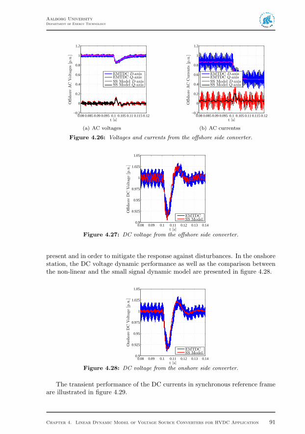
ii
“Thesis” — 2012/11/2 — 9:02 — page 91 — #91 ii
ii
ii
Aalborg UniversityDepartment of Energy Technology
0.08 0.085 0.09 0.095 0.1 0.105 0.11 0.115 0.12−0.2
0
0.2
0.4
0.6
0.8
1
1.2
t [s]
Offshore
AC
Voltages
[p.u.]
EMTDC D-axisEMTDC Q-axisSS Model D-axisSS Model Q-axis
(a) AC voltages
0.08 0.085 0.09 0.095 0.1 0.105 0.11 0.115 0.12−0.2
0
0.2
0.4
0.6
0.8
1
1.2
t [s]
Offshore
AC
Currents
[p.u.]
EMTDC D-axisEMTDC Q-axisSS Model D-axisSS Model Q-axis
(b) AC currentss
Figure 4.26: Voltages and currents from the offshore side converter.
0.08 0.09 0.1 0.11 0.12 0.13 0.140.9
0.925
0.95
0.975
1
1.025
1.05
t [s]
Offshore
DC
Voltage[p.u.]
EMTDCSS Model
Figure 4.27: DC voltage from the offshore side converter.
present and in order to mitigate the response against disturbances. In the onshorestation, the DC voltage dynamic performance as well as the comparison betweenthe non-linear and the small signal dynamic model are presented in figure 4.28.
0.08 0.09 0.1 0.11 0.12 0.13 0.140.9
0.925
0.95
0.975
1
1.025
1.05
t [s]
Onshore
DC
Voltage[p.u.]
EMTDCSS Model
Figure 4.28: DC voltage from the onshore side converter.
The transient performance of the DC currents in synchronous reference frameare illustrated in figure 4.29.
Chapter 4. Linear Dynamic Model of Voltage Source Converters for HVDC Application 91

ii
“Thesis” — 2012/11/2 — 9:02 — page 92 — #92 ii
ii
ii
Aalborg UniversityDepartment of Energy Technology
0.08 0.09 0.1 0.11 0.12−1.2
−1
−0.8
−0.6
−0.4
−0.2
0
0.2
0.4
0.6
0.8
t [s]Onshore
AC
Currents
[p.u.]
EMTDC D-axisEMTDC Q-axisSS Model D-axisSS Model Q-axis
Figure 4.29: Converter currents in the onshore station in synchronous reference frame.
4.8.2.2 DC Bus Voltage Reference Variation
The results presented above illustrate the performance of the VSC-HVDCsystem under power disturbances. A different scenario can be explored whenconsidering the DC voltage reference variation on the onshore side. By this means,the evaluation of the consequences of such change at the offshore can be performedanalysing the offshore AC voltage at the point of common coupling. The resultsfrom figure 4.30 show the decoupling between the offshore AC side and the DCside perturbation. This phenomenon is related with the feedforward compensationin the current controller. The small signal model performance is also comparablewith the EMTDC simulation.
0.08 0.085 0.09 0.095 0.1 0.105 0.11 0.115 0.12−0.2
0
0.2
0.4
0.6
0.8
1
1.2
t [s]
Offshore
AC
Voltages
[p.u.]
EMTDC D-axisEMTDC Q-axisSS Model D-axisSS Model Q-axis
(a) AC voltages
0.08 0.09 0.1 0.11 0.12 0.13 0.140.9
0.925
0.95
0.975
1
1.025
1.05
t [s]
Offshore
DC
Voltage[p.u.]
EMTDCSS Model
(b) DC currentss
Figure 4.30: Offshore converter voltages at the point of common coupling and DC busunder DC voltage set point variation.
At the onshore side, the converter presents the direct voltage control. The PIcompensation is able to keep the system stable as well as promote zero error atthe steady state. The overshoot and settling time can be design to lead the timeresponse to a desired shape.
For the model validation comparison, the EMTDC model was compared withthe small signal model given by the linearisation of the current and voltage loops.
92 Chapter 4. Linear Dynamic Model of Voltage Source Converters for HVDC Application

ii
“Thesis” — 2012/11/2 — 9:02 — page 93 — #93 ii
ii
ii
Aalborg UniversityDepartment of Energy Technology
The state space model of the system is provided in the main text. The dynamicbehaviour of the offshore and onshore DC voltage are compared in figure 4.31.
0.08 0.09 0.1 0.11 0.12 0.13 0.140.9
0.925
0.95
0.975
1
1.025
1.05
t [s]
Onshore
DC
Voltage[p.u.]
EMTDCSS Model
Figure 4.31: Onshore converter voltages at the DC bus under DC voltage set pointvariation.
Chapter 4. Linear Dynamic Model of Voltage Source Converters for HVDC Application 93

ii
“Thesis” — 2012/11/2 — 9:02 — page 94 — #94 ii
ii
ii
Aalborg UniversityDepartment of Energy Technology
94 Chapter 4. Linear Dynamic Model of Voltage Source Converters for HVDC Application

ii
“Thesis” — 2012/11/2 — 9:02 — page 95 — #95 ii
ii
ii
CHAPTER5Robust Control TechniquesApplied in DC Transmission
Systems
The energy transfer from offshore to onshore by means of HVDC is highlydependent of the controls performance. On the offshore, the weakness of the
grid is a drawback for the engineering. On the onshore side, the control of DCvoltage is affected by the power variations as well as by the grid conditions. Inboth cases, the assurance for stability is a must, and with the requirements fromthe grid codes, not only the stability is compulsory, but the dynamic performanceof the converter is a essential role, as well.
This chapter investigates the stability and performance of the voltage sourceconverters when they are interconnected by DC cables. The aim is to compare thestability and dynamic performance of the converter in the cases where they haveclassical proportional-integral controllers and robust controllers. The comparisonis accomplished by means of frequency domain eigenvalue position.
First of all, an introduction about the control design and specification in thefiled of robust control is presented and how the adopted control strategy (µ-synthesis) fits for high voltage DC applications. Using the linear models fromthe previous chapter, the eigenvalue position assessment of each of the station isevaluated considering system uncertainties such as different short circuit ratios,DC voltages and processed power.
The sensitivity of the system is tested in the complex plane by varying theparameters of the system. Both controllers, the PI and the robust control havetheir sensitivity compared by relating the rate of change of the position of theireigenvalues in the complex plane. The stability assessment for a point-to-pointVSC-HVDC and for multiterminal case with four terminal are explored in thefinal sections.
95

ii
“Thesis” — 2012/11/2 — 9:02 — page 96 — #96 ii
ii
ii
Aalborg UniversityDepartment of Energy Technology
5.1 General Feedback Control System Design
Automatic control is an interdisciplinary theory which has become importantin the power system and in power electronics. Historically, the control theory hasbeen divided in two main branches: classical and modern control [49]. Some au-thors mention post-modern categories to differentiate some recent techniques [54].
Classical control is still in use but it finds some limitations when the treatmentof multiple-input multiple-output (MIMO) systems is required. Modern controltheory has become popular after the 60s with the introduction of digital computersdue to its processing power [50]. Inside modern control theory, many other sectionare, nowadays, part of the picture of control concepts. They are itemized below.
• Adaptive control
• Hierarchical control
• Intelligent control
• Optimal control
• Robust control
• Stochastic control
This work is based in the robust control theory and it aims for its applicationfor grid connected voltage source converter in high voltage DC transmission. Withthis focus, it is possible to use the general feedback control architecture fromfigure 5.1.
G(s)
Plant
Filter
H(s)
Reference C(s)Controller
Sensor
K(s)
Disturbance
Noise
Output
ParameterUncertainty
Control Level Plant/Harware Level
r(t)
e(t) u(t)
n(t)
y(t)
d(t)
w(t)
Figure 5.1: General control architecture for a feedback dynamic system.
The controller C(s) is designed aiming for basically five performance criteria:
• Reference tracking
• Disturbance attenuation
• Noise rejection
96 Chapter 5. Robust Control Techniques Applied in DC Transmission Systems

ii
“Thesis” — 2012/11/2 — 9:02 — page 97 — #97 ii
ii
ii
Aalborg UniversityDepartment of Energy Technology
• Less control energy
• Parameter uncertainties effect mitigation
In the classical control theory, the controller C(s) can be design with thecompromise among any of the four performance criteria. It is well know, however,that the emphasis in one of the them leads to depreciation of the others [51].Moreover, the influence of the uncertainties in the nominal model is not so oftenconsidered even in some of the modern control design methods.
In a connection of voltage source converter and the utility grid, the uncer-tainties are confidently impose over the performance of power processing of suchpower electronic devices. In this case, it is possible to cite, for example, thegrid AC voltage, converter DC voltage (which can vary in case of multiterminalDC connection based on droop control presented in the previous chapter) andconverter processed power.
As a common practice in power system operation, the scheduling of power setpoints is sent to the converter station, and its control is designed considering thisoperating points settled by the system operators [52]. This process is made byusing linearisation of the system. More than just the control design, the dynamicmodel of the system can assess its stability and dynamic performance.
However, even in the time frame between two consecutive set point updates,the entire power system presents variations. Those variations can be, for example,changes in the grid voltage values, load changing, and in case of wind powerconnection, fluctuation in the energy production by the wind farms connectedto the grid. Those variations can change the properties of the system and haveinfluence in the performance of the power delivered from the HVDC converters.
Considering a knowledge of the uncertainty and the effect of disturbances inthe VSC devices, the analysis of the system using structured singular values as wellas the control design by means of µ-synthesis can, intrinsically, be in accordancewith uncertainty unification in the system. This enhances the performance overthe gain scheduled controller, in case of small time scale, and on the same time,decrease the complexity of the system in comparison with more complex adaptivesystems.
Another issue is directly related with the system performance analysis. Withsuch methodology which quantifies the impact of the uncertainties already in themodelling process, the effectiveness of the controller and disturbance mitigationcan be measured by the use of structured singular values and worst case analysisrelated with induced system norm [53, 54].
One chapter in the appendix shows a brief introduction about the theoryand methodology adopted by µ-synthesis and analysis. There, one can find thedescription of uncertainty modelling procedure, linear fraction transformation aswell as a summary regarding the design algorithm and optimisation process relatedin the control structure definition.
For the control design procedure and performance analysis of the system pre-
Chapter 5. Robust Control Techniques Applied in DC Transmission Systems 97

ii
“Thesis” — 2012/11/2 — 9:02 — page 98 — #98 ii
ii
ii
Aalborg UniversityDepartment of Energy Technology
sented by figure 5.1, the following steps are required:
1. Modelling of the plant G(s)
2. Validation of the plant model
3. Modelling of uncertainties
4. Control design
5. Performance validation
6. Retuning of the control settings (if required)
The following section follows the steps presented above. The plant modeluses the well known process of linearisation and small signal modelling usingstate space model. For the model validation, the comparison between the statespace dynamic model and the EMTDC time domain simulation are evaluated foracceptance of the linear model. From the last chapter, one can find the derivationfor the dynamic model for offshore and onshore converters as well as wind powerplant, DC cable and grid.
The control design is a intermediate process, in which the theory behind it isrefereed to [53, 54, 51]. The subitems related to control order reduction as wellas weighting functions and control performance evaluation can also be found inthe references.
5.2 Justification of Optimal Robust Control De-sign for HVDC Applications
In the interconnection of a HVDC system and a wind farm with the gridutility, the converters are able to control the variables in each the control modesare selected for: the DC voltage, in case of the onshore converter, and AC, on theoffshore side. Considering for example the onshore side converter, one can dividethe system in four main modules; three belonging to description of one stationand the other one as the grid.
The utility grid is a combination of multiples machines, cables, transmissionlines and loads. It presents a very complex dynamics, however, this work simplifiesthe grid behaviour by a simple Thevenin model.
For the converter viewpoint, using the grid simplification, the behaviour ofthe controllers inside the HVDC onshore stations are highly affected by the grid.Using the simplified Thevenin model, the stiffness and weakness of the grid canbe evaluated. This characteristic can be included in the model by means of theseries impedance LG and RG. The variation of the values of the short-circuitration in the grid can, in some cases, emulated adversities in the grid and those
98 Chapter 5. Robust Control Techniques Applied in DC Transmission Systems

ii
“Thesis” — 2012/11/2 — 9:02 — page 99 — #99 ii
ii
ii
Aalborg UniversityDepartment of Energy Technology
ones can affect the converter dynamics by means of variation in the voltages andcurrents in the point of common coupling.
In the case of a HVDC connection, looking from the DC side of the HVDCconverter, the offshore system is a power source with a certain dynamics. Again,the incoming power from the offshore sides interacts with the whole rest of thesystem in a interconnected manner. Figure 5.2 helps to illustrates, in a simpleblock diagram, the interconnection among the AC side, HVDC converter and DCside.
vDC(t)
vGDQ(t)
ω
iDQ(t)
Con
vert
er C
urre
nt L
oop
i*
iDQ(t)
vDQ(t)
Gri
dC
urre
nt iGDQ(t) if DQ(t)vGDQ(t) HF
Filte
r
ωtθ
ΔG
ΔCC
Con
vert
er D
C
Volta
ge L
oop
uDQ(t)
ΔDC
Po(t)
vDC(t)θ
Figure 5.2: Block diagram of the modules of onshore converter with its uncertainties.
As a simplification manner, all the spoiled dynamics present in both, AC sideand DC grid sides, can be represented as disturbances for the converter controllers.For the utility grid, for example and as it was mentioned before, the weaknessand stiffness can be emulated by variations in the grid impedance.
From the models presented in the previous chapter, such values are treated assystem parameters. The changes in the those parameters are modelled as modelparameter variation using the block ∆G in the figure 5.2.
Similar approach can be used for the power variations where, not only as ainput disturbance for the system, but as a consideration in the operating pointvariation. In the linearisation process presented in the previous chapter, theoperating point was crucial in the determination of some parameter values andthe variation of such conditions can be sensitive to the converter controllers.
The representation of the system according to the figure 5.2 can drive theattentions to a method in the modern control theory called µ-synthesis wheresimilar framework is te basic approach for design robust control for system underuncertainties.
Uncertainty in control systems assigns to the model imperfections as well asdifferent forms of disturbances in which a system can be under effect. The for-mer represents the discrepancies between the nominal mathematical model andthe real physical system. For the current application, the variations the gridimpedances and operating points. The last case references to the unpredictablenature of the disturbance bounded inputs. One can refer to power variations, forexample. The trade-off represented by the uncertainty modelling in the classical
Chapter 5. Robust Control Techniques Applied in DC Transmission Systems 99

ii
“Thesis” — 2012/11/2 — 9:02 — page 100 — #100 ii
ii
ii
Aalborg UniversityDepartment of Energy Technology
control theories are, nowadays, solved by new control techniques based on theoptimal robust techniques, in case, the µ-synthesis.
5.3 Robust Control: Design and Specification
The adopted control design method presents the advantage in simplify somedynamics of the system by means of system parameter variation and bounded in-put disturbances. The design method requires details in optimisation techniquesrelated with non-convex optimisation, linear fraction transformation, structuredsingular values and system norms. Those concepts are commonly used in moderncontrol technique and cab be found in [53] and [54]. Details regarding implemen-tation are described in [51]. Few definitions and brief details are given in theappendix. The objective of this is work is to to concentrate the efforts in methodsfor the control design, but simplify the description of the dynamics of a complexsystem and apply a robust technique to improve the converter dynamics.
The process of the µ-synthesis lies on the principle of output feedback control.The main objective is find a controller C(s) such that the performance of thesystem, considering the plant and the uncertainties, is satisfied for determinedrange of variation of the uncertainty block ∆. Figure 5.3.
G(s)
Plant
Δ
Uncertainty Block
u(t)
w(t)
y(t)
z(t)
C(s)
Controller
r(t)
Figure 5.3: Simplified representation of feedback system with augmented plant.
The preliminary step is describe the augmented plant in terms of input/outputstate space model considering the uncertainty block ∆. This representation is anextension of state space model of the system including the inputs w(t) and outputsz(t) related to the uncertainty block. This characterisation of the dynamic systemis written in equations (5.1), (5.2) and (5.3).
x(t) = Ax(t) +B1z(t) +B2u(t) (5.1)
z(t) = C1x(t) +D11z(t) +D12u(t) (5.2)
y(t) = C2x(t) +D21z(t) + 222u(t) (5.3)
(5.4)
According to (5.4), the matrices A, B2, C2 and D22 belong to the nominal
100 Chapter 5. Robust Control Techniques Applied in DC Transmission Systems

ii
“Thesis” — 2012/11/2 — 9:02 — page 101 — #101 ii
ii
ii
Aalborg UniversityDepartment of Energy Technology
state space model for the plant G(s) with no uncertainties.
With the uncertainty model described in the mathematical form from (5.4),it is necessary to determine the performance specification. This stage is directrelated to the requirements derived from the grid prerequisites, standards andcodes. In the robust optimal control, the specification is translated to the optimi-sation by means of weight functions which can be scalar, transfer functions andeven additional dynamic systems.
The choice of the weight functions is, usually, the drawback in the designprocess [51]. The trial and error is some times the unique solution, however, insome cases there are methods for designing the functions. The direct methodfor inspection, method, is though, used for define the performance criteria forthe high power converter in the HVDC connection. For all the control loopsthe same methodology is applied. Few parameters change in order to fulfil therequirements. Generally, two weight transfer functions are included in the system,one for the reference tracking performance and another included to filter andbound the control command. They are, respectively Wp and Wu. Figure 5.4shows the uncertainty plant been controlled by the augmented controller withintegral additional integral action and the position of the weighting functions forthe design.
G(s)
Plant
Δ
Uncertainty Block
u(t)
w(t)
y(t)
z(t)
C(s)
RobustController
r(t)1s
PIController
Wp(s)
zp(t)
Wu(s)
zu(t)
Figure 5.4: General robust weighting architecture for the design of robust control bymeans of µ-synthesis.
The first weight function Wp shapes the time response of the error. Into it,the requirements regarding settling time and damping factor are specified. ThePI controller is included just after the error calculation for guaranteeing zero errorat the steady state as well as alleviates the iteration process during the controldesign optimisation.
The output of the control command is weighted as well. This function isapplied to put the constraints in the optimisation such that the control effort toachieve the specification requirements have low control energy. For the switcheddevices, in addition, this function can be design with filtering characteristics. Forthe current controller for example, the weight function can have a cut-off frequencysuch that the command signal will not face double crossings in the modulator.
The final stage is the control optimisation algorithm where the state space
Chapter 5. Robust Control Techniques Applied in DC Transmission Systems 101

ii
“Thesis” — 2012/11/2 — 9:02 — page 102 — #102 ii
ii
ii
Aalborg UniversityDepartment of Energy Technology
model of the controller is obtained. The objective function describes the seek fora controller C(s) such that the H∞-norm of the augmented system structuredsingular values of the transfer matrix between the outputs zp and zu and theinputs is minimised. In layman’s words, the H∞-norm represents the worst caseperformance that a system can present. The structure singular values, are in away, related to the eigenvalues of the state space dynamic system considering therange of variation in the uncertainty matrix ∆.
This optimisation process requires iterations, usually the D−K iterative pro-cess [53] and , first of all, do not guarantee uniqueness of the solution due to thenon-convexity of the system. Another disadvantage is that it does not guaranteeconvergence.
5.3.1 Uncertainty Model
The uncertainties are intrinsic in the main blocks from figure 4.5. The consid-ered uncertainties for the dynamic system are input voltages and the short circuitratio (representation of stiffness of the grid), for the grid current dynamic block;active and reactive power for the converter current block and grid frequency canpresent variation, as well. For quantitative analysis, the voltages, SCR and con-verter DC voltages and processed powers are considered to vary according to thevalues presented by table 5.1.
Variable/Parameter Uncertainty Value Variable
Grid AC Voltage ±10% δVAC
Grid frequency ±1% δwGrid SCR 7 to 3 δLG and δRG
DC Voltage ±3% δVDC
Converter Power ±25% δP and δQ
Table 5.1: Parameter uncertainties for current loop analysis.
5.3.2 The Inner Loop with Uncertainties
From figure 5.2, the uncertainty matrices are the representation of the varia-tions in the system. For the inner current controller viewpoint, the uncertaintiesare going to be reflected in variations the power transfer set point. Due to thepossibility to measure disturbances, the performance of the inner current con-troller against disturbances is improved by the feedforward compensation. As aresult, the model of the inner current controller considering the uncertainties cabe considered such as is illustrated in figure 5.5.
The uncertainty from the DC voltage value is the unique variational blockpresent, since that it is considered the feedforward action. Such condition whereconsidering the DC voltage variation is a prediction for multiterminal connection,since, in this kind of system topology the changes in the DC voltage are present.
102 Chapter 5. Robust Control Techniques Applied in DC Transmission Systems

ii
“Thesis” — 2012/11/2 — 9:02 — page 103 — #103 ii
ii
ii
Aalborg UniversityDepartment of Energy Technology
1s
1LC
ΔmDQ(t) ΔiDQ(t)VDC0.5
δVDCz12(t) w12(t)
Figure 5.5: Simplified block diagram of the inner current plant with uncertainties.s
Assuming the model from figure 5.5, the augmented state space model withsystem uncertainties is given by equations (5.5), (5.6) and (5.7)
xDQ(t) =
[0 00 0
]xDQ(t) + [−1]wDQ(t) +
[−VDC2
]uDQ(t) (5.5)
zDQ(t) =
[0 00 0
]xDQ(t) + [0]wDQ(t) + [1]uDQ(t) (5.6)
yDQ(t) =
[ 1LC
0
0 1LC
]+ [0]wDQ(t) + [0]uDQ(t) (5.7)
5.3.3 DC Voltage Loop with Uncertainties
The DC voltage model considers the variations in power transfer from the ACto DC side or vice versa. In the model, the uncertainty of the DC voltage controlleris direct connected to the power variations. By this means, the δ components ofthe uncertainty matrix ∆ have the uncertainties in voltage and currents processedby the converter station. Figure 5.6 illustrates the DC voltage plant model forthe DC loop plant model with the system uncertainties.
IDQ
δIDQ
ΔmDQ(t)
MDQΔiDQ(t)
δMDQ
0.5 1s
1CDC
ΔvDC(t) 2VDCΔvDC(t)Δv2
I DC
δ IDQ
iDC(t)
z12(t) w12(t)
z34(t) w34(t)
z5(t)
w5(t)
Figure 5.6: DC voltage loop plant considering the uncertainties in the model.
At the AC side of the converter, the range of variation of the current inthe synchronous reference frame, iDG, is a result of variations in the power andvoltages at the power of common coupling. The DC current value, is then, acombination of the modulation indexes and currents. The modulation indexesconsiderer the feedforward components as well. By the linearised block diagramfrom figure 5.6, the state space model which includes the uncertainties of the DCloop plant is given by (5.8), (5.9) and (5.10)
Chapter 5. Robust Control Techniques Applied in DC Transmission Systems 103

ii
“Thesis” — 2012/11/2 — 9:02 — page 104 — #104 ii
ii
ii
Aalborg UniversityDepartment of Energy Technology
xDC(t) = [0]xDC(t) +[
0.5 0.5 0.5 0.5 −1]wDC(t) +
[MD MQ ID IQ −1
]uDC(t) (5.8)
zDC(t) = [0]xDC(t) +[
0 0 0 0 0]wDC(t) +
[1 1 1 1 1
]uDC(t) (5.9)
yDC(t) =
[1
CDC
]xDC(t) +
[0 0 0 0 0
]wDC(t) +
[0 0 0 0 0
]uDC(t) (5.10)
5.3.4 AC Voltage Loop with Uncertainties
The control of the voltage at the AC side of the converter i required at theoffshore station. As the same uncertainty variable presented in the DC voltagecontrol loop, the power variation is the uncertainty for the system where the ACvoltage control mode is the compensation strategy.
Indirectly presented in the model, the uncertainty is power is reflected in themodel by means of consideration in the voltage and current level in the convertermodel. The voltage is the control variable, and the AC currents are the inputdisturbances. By then, the uncertainties are included the disturbance input as adefinition of the variational variable which serves as input for the robust controldesign algorithm. Figure 5.7 illustrates the uncertainty plant model for the ACvoltage loop of the converter station.
Δif DQ(t) ΔvGDQ(t)ΔiGDQ(t)IGDQ
δIGDQ
z12(t) w12(t)
HF
Filte
rθ
ΔiDQ(t)Figure 5.7: AC voltage loop plant considering uncertainties in the system.
The augmented plant model presented in figure 5.7 have the state model,model with the framework from the equation (5.4). The dynamic state spaceequation model is represented by the state space equation of the high frequencyfilter in (4.47).
5.4 Control Design Performance Specification
5.4.1 Inner Current Control Loop
The performance specification for the inner current controllers from the off-shore and onshore converter have the same parameters. The first criterion is
104 Chapter 5. Robust Control Techniques Applied in DC Transmission Systems

ii
“Thesis” — 2012/11/2 — 9:02 — page 105 — #105 ii
ii
ii
Aalborg UniversityDepartment of Energy Technology
regarding reference tracking. For this purpose, the extra integrator was includedin the loop to guarantee zero error in steady-state. This action suppress the ne-cessity in forcing the optimisation algorithm in finding an optimal controller suchthat there is a integrator in its structure. In some cases, more constraints in theoptimisation process can drive the algorithm to divergence.
The second consideration in the control design for the converters AC currentsare related with the settling time. Due to the limitation in bandwidth, the currentcontroller is set to have 390 Hz of bandwidth. This value is five times less than theswitching frequency and guarantee compensation for lower harmonics, if required.The damping factor is chosen to be 1√
2.
The last specification considers the filtering and saturation prediction of thecontrol command error. The first is required for the proper modulation perfor-mance and the former, guarantees that the converter operates at the consideredlinear region. All the requirements are summarised in table 5.2.
Parameter Value Unit Comment
Bandwidth 390 Hz Assumed
Damping Factor 1√2
Assumed
Filter Bandwidth 975 Hz Assumed
Control Command Saturation Gain 1.0 Assumed
Table 5.2: Summary of the requirements specified for the current control robust design.
For the robust control design, the specification presented in table 5.2 can betranslated to weight functions. For the performance specification, the Wp functionis selected and for the control command compensation Wu. Each of the objectivesrelated with the specification requirements are itemized below:
Wp: Performance weight function with high gains in low frequency for the refer-ence tracking performance. The settling time is defined by the bandwidthset by the cut-off frequency. The damping is also specified by the loop shapeof the function.
Wu: Weight for the control output command guarantees saturation avoidanceand filtering of the high harmonic contents. This action is required to assurethe absence of double crossings in the modulator.
The frequency response of the selected weight functions are illustrated by thebode plots presented in figures 5.8(a) and 5.8(b).
5.4.2 DC and AC Outer Voltage Control Loops
For the onshore converter the DC voltage control loop is present while inthe offshore sites the AC voltage control loop promotes voltage support to theconnection with the wind farms. The connection between the outer controllers andthe inner current control is design such that the dynamic decoupling is assured.
Chapter 5. Robust Control Techniques Applied in DC Transmission Systems 105

ii
“Thesis” — 2012/11/2 — 9:02 — page 106 — #106 ii
ii
ii
Aalborg UniversityDepartment of Energy Technology
101
102
103
104
−20
−10
0
10
20
30
40
Frequency [Hz]
Magnitude[dB]
(a) Reference tracking (Wp).
103
104
−15
−12.5
−10
−7.5
−5
−2.5
0
2.5
5
Frequency [Hz]
Magnitude[dB]
(b) Control Command (Wu).
Figure 5.8: Weighting functions for the performance specifications in the inner currentcontroller.
For the outer loop control specification, the weight functions for the control designhave the same frequency response presented in figures 5.8(a) and 5.8(b). However,different parameters define the settling times and control command weights.
For simplification in the design and simulations, it is considered that all thevoltage source converters in the same are sized with the same parameters pre-sented in table 4.1 and 4.2. Both, outer loops, the DC and AC voltage loops, areconsidered to have the same specification which is described in table 5.3.
Parameter Value Unit Comment
Badwidth 78 Hz Assumed
Damping Factor 1√2
Assumed
Filter Bandwidth 390 Hz Assumed
Control Command Saturation Gain 1.0 Assumed
Table 5.3: Summary of the requirements specified for the current control robust design.
5.5 Control Performance Comparison in a Point-to-Point VSC-HVDC Transmission
The previous chapter presented the results of the model validation in a point-to-point HVDC connection. There, the accuracy of the model was tested againstthe EMTDC simulations. The effort in making a precise state space model lies onthe advantage in the allowance in the assessment of the frequency domain analysisof the dynamic system.
The usage of the state space model derived previously allows the frequencydomain analysis by means of robust performance and system sensitivity. The firstconsiders the evaluation of the eigenvalue position in the complex plane. Thedamping and eigenvalue frequencies define the main characteristic the dynamic
106 Chapter 5. Robust Control Techniques Applied in DC Transmission Systems

ii
“Thesis” — 2012/11/2 — 9:02 — page 107 — #107 ii
ii
ii
Aalborg UniversityDepartment of Energy Technology
performance.
The sensitivity analysis is related with system parameter variations. Theevaluation of the system operating point and how the changes in its parameterscan affect the stability performance is defined by the rate of eigenvalue positionvariation.
5.5.1 Model Performance under Active Power Variation
In the point-to-point transmission case, the control of power is directly per-formed by the wind power plants. The HVDC links acts a corridor. For thisstudy case, the performance of the HVDC controllers are evaluated by means ofdisturbance rejection, since, the incoming power is modelled with such behaviour.
In the offshore shore side, the stiffness of the AC voltage control promotesbetter operation conditions for the wind turbines connected by the AC collection.The performance under the input power disturbances is a reasonable of the controlquality.
At the offshore side, the power variation promotes changes in the DC voltagewhich directly affects the current controller states. The limited range of operationof a HVDC converter is a key point for determination of the final cost of thesystem. Allowing the operation of the DC voltage in higher DC levels requiresmore costly converter station. The second point is related with the DC cableswhich are, as well, sensitive to voltage operating conditions.
For this study case, a point-to-point HVDC connection transmission systempresents two operating conditions. The initial case consider the classical PI con-troller. The second case makes use of the robust control design by means of theµ-synthesis. The test case consider a initial condition for the offshore power de-liver at 0.8660 pu of active power. At the onshore operation the reactive currentreference is set to be 0.5 pu. At the offshore side, the AC voltages have their timedomain simulation response given by figure 5.9.
0 0.005 0.01 0.015 0.02 0.025 0.030.6
0.7
0.8
0.9
1
1.1
t [s]
D-A
xis[p.u.]
EMTDCSS Model
0 0.005 0.01 0.015 0.02 0.025 0.03−0.25−0.15−0.05
0.050.150.250.35
t [s]
Q-A
xis[p.u.]
EMTDCSS Model
(a) AC voltage PI controller performance
0 0.005 0.01 0.015 0.02 0.025 0.030.6
0.7
0.8
0.9
1
1.1
t [s]
D-A
xis[p.u.]
EMTDCSS Model
0 0.005 0.01 0.015 0.02 0.025 0.03−0.25−0.15−0.05
0.050.150.250.35
t [s]
Q-A
xis[p.u.]
EMTDCSS Model
(b) AC voltage robust controller performance
Figure 5.9: Control performance evaluation for wind power variation.
Chapter 5. Robust Control Techniques Applied in DC Transmission Systems 107

ii
“Thesis” — 2012/11/2 — 9:02 — page 108 — #108 ii
ii
ii
Aalborg UniversityDepartment of Energy Technology
The three main characteristics between the figures 5.9(a) and 5.9(b) are re-lated to the deepest point, settling time and overshoot. The performance of therobust boosted the dynamics of the system. The overshoot, which can affect thesizing of the offshore components, is highly improved by the robust controller asa combination of fast current controller and higher order control characteristic.
The DC voltages for the offshore and onshore sides play a very important rolein the operation of the HVDC system. The DC voltage controller, as previouslymentioned, is placed at the onshore converter controller. By this means, theloose control at the onshore side converter can compromise the operation of theoffshore converter. Due to the non-controllability of the offshore DC voltage andalso due to the effect of the DC cable dynamic the converter, the DC voltageat the sending-end converter is directly under influence of the onshore converterstation. The improvements presented by the robust control in the DC voltagecompensation is illustrated by the time domain simulation from figure 5.10.
0 0.01 0.02 0.03 0.04 0.05 0.06 0.070.85
0.9
0.95
1
1.05
t [s]
DC
Voltage[p.u.]
EMTDCSS Model
(a) Onshore DC voltage PI controller perfor-mance
0 0.01 0.02 0.03 0.04 0.05 0.06 0.070.85
0.9
0.95
1
1.05
t [s]
DC
Voltage[p.u.]
EMTDCSS Model
(b) Onshore DC voltage robust controller per-formance
Figure 5.10: Control performance evaluation for wind power variation.
The refined controller promoted by the onshore DC voltage controller is di-rectly measured by the overshoot mitigation during the transient condition. Thesettling time between the response of the classical PI controller and the robustaugmented controller are approximately the same.
At the offshore side, the improvements in overshoot voltage is as well improved.The time domain simulation results for the offshore side converter station areillustrated by the figure 5.11.
5.5.2 Model Performance under DC Reference Variation
The DC voltage reference changes in a HVDC transmission is a previous studyfor predicting the roust performance of the HVDC system in the multiterminalconnection. The evaluation of the robust control over the proportional-integralcompensator are presented in figure 5.12.
As the same improvements presented for disturbance rejection in the previous
108 Chapter 5. Robust Control Techniques Applied in DC Transmission Systems

ii
“Thesis” — 2012/11/2 — 9:02 — page 109 — #109 ii
ii
ii
Aalborg UniversityDepartment of Energy Technology
0 0.01 0.02 0.03 0.04 0.05 0.06 0.070.85
0.9
0.95
1
1.05
t [s]
DC
Voltage[p.u.]
EMTDCSS Model
(a) Offshore DC voltage PI controller perfor-mance
0 0.01 0.02 0.03 0.04 0.05 0.06 0.070.85
0.9
0.95
1
1.05
t [s]
DC
Voltage[p.u.]
EMTDCSS Model
(b) Offshore DC voltage robust controller per-formance
Figure 5.11: Control performance evaluation for wind power variation.
0 0.01 0.02 0.03 0.04 0.05 0.06 0.070.95
0.975
1
1.025
1.05
1.075
1.1
EMTDCSS ModelReference
(a) Onshore DC voltage PI controller perfor-mance
0 0.01 0.02 0.03 0.04 0.05 0.06 0.070.95
0.975
1
1.025
1.05
1.075
1.1
EMTDCSS ModelReference
(b) Onshore DC voltage robust controller per-formance
Figure 5.12: Control performance evaluation for wind power variation.
case, the robust controller could better track the reference. The settling time doesnot present significant improvements in both of the cases. The main contributionthat makes the robust controller a better candidate is related with the overshootmitigation. While the overshoot rate from the PI controller is around 30 to 40%,the robust controller performance presents a overshoot close to 5%.
5.5.3 System Performance under Grid Impedance Varia-tion
The grid impedance variation is a test study which aims to be a preliminaryassessment for grid faulted conditions. The variation in the short circuit ratio ofthe system can emulate the changes in the interconnected utility grid such as linetrips for example.
The analysis is performed using the EMTDC simulation. The system is ini-tially operation at 0.8660 pu of active power. At the onshore operation the reac-
Chapter 5. Robust Control Techniques Applied in DC Transmission Systems 109

ii
“Thesis” — 2012/11/2 — 9:02 — page 110 — #110 ii
ii
ii
Aalborg UniversityDepartment of Energy Technology
tive current reference is set to be 0.0 pu. The grid impedance present a suddenchange which reflects a variation of the short ratio from 7 to 3. The simulationresults which consider this scenario are shown in figure 5.13.
0 0.01 0.02 0.03 0.04 0.05 0.06 0.070.9
0.92
0.94
0.96
0.98
1
1.02
1.04
1.06
Instant of SCR Variation
(a) DC voltage time domain simulation for PIController.
0 0.01 0.02 0.03 0.04 0.05 0.06 0.070.85
0.9
0.95
1
1.05
1.1
1.15
1.2
Instant of SCR Variation
(b) DC voltage time domain simulation forRobust Controller.
Figure 5.13: DC voltage time response for variation in the utility grid short circuitratio.
The variation of the grid impedance clearly affects the DC voltage. The robustcontroller performance is, again, higher in comparison which the PI controller.The effect of the grid impedance variation is, as well, promoted by the performanceof the synchronisation loop presented in the phase-locked loop. The influence ofthe synchronism delay effect of the phase-lock loop is not evaluated in this work.
110 Chapter 5. Robust Control Techniques Applied in DC Transmission Systems

ii
“Thesis” — 2012/11/2 — 9:02 — page 111 — #111 ii
ii
ii
Conclusions
The increase in size and power capacity of the wind turbines and the windavailability in the sea sites, moved the wind farms from the land to offshore.
This action forced the seek for new technologies which could be able to transmitthe bulk amount of energy. Due to the lack of reactive power compensation andloss levels, the HVDC solution came to overcome the traditional HVAC. Alliedwith the developments in the power semiconductors and converter topologies, thevoltage source converters are able to provide this interconnection between thewind farms and shore by means of DC.
This possibilities in linking more than one wind farms and more than onegrid utility using HVDC is an envisage and the static analysis presented in firstthe part of this work proposed a methodology for operating a DC network bymeans of droop control. The optimisation algorithm is applied in a classicalload flow technique and depending on the determination of the cost function, thefunctionality of the multierminal DC system can fulfil some requirements of thegrid utilities.
The main results are based in the choice of two main objectives: loss minimi-sation an dispatch optimisation. In the minimisation of losses, the cable modelswere simplified and the loss model of the two-level converter were included in theiterative method. In the dispatch problem, the classical revenue quadratic costfunction is tested against the minimisation of the dispatch error. The advantagein limiting the error between the scheduled dispatch in the last case is comparedwith the improvements in operating the system with smaller losses in the firstcase.
The dynamic viewpoint in a HVDC transmission is provided by means ofsmall signal analysis of the converter. The operation of the control modes, one foronshore and the other for offshore, were modelled and the results were comparablewith the time domain simulations provided by the EMTDC model. The modellingpart is a important stage for the derivation of the complete model of the converterplant, since the control definition is highly dependent of the model accuracy whenit is connected with the real system.
The simplification of the dynamics of the system using structure uncertaintymodels and its use for the robust design of the converter controllers presentedpromising benefits. The main test cases are able to demonstrate the improvementsin the dynamic operation of a point-to-point VSC-HVDC system under transientconditions.
111

ii
“Thesis” — 2012/11/2 — 9:02 — page 112 — #112 ii
ii
ii
Aalborg UniversityDepartment of Energy Technology
Nowadays, many options are available for the robust control design. Theµ-synthesis is one them. The control design in this work, by itself, does notpresented novelties related with algorithm developments. The contribution statesin the definition of the weight function for the design. Usually, such task involvestrial and error process.
The study of variation in the power delivered from the wind farms, the voltagereference order variation as well as grid impedance deviations are tested. The firstcase consider a real scenario predicting the variability of the wind behaviour. Thesecond case gives insights regarding the possibilities of multiterminal connection.In this case, the connection with the static optimisation is in the fact that thechanges in the DC voltage references, in one of the stations in the DC grid, acts asdisturbance for the other converters where the droop controllers are in operation.
The changes in the grid impedance emulates the possible discrepancies inthe conditions of the utility grid. Line tripping is one of the possible real caseswhich can endorse the accomplished study. The results are able to show thatthe augmented controller, design by means of µ-synthesis performs in a bettercondition than the classical PI controller.
Main Contributions
In the operation of a multiterminal VSC-HVDC, some control methods areproposed in the literature. The droop control is one of them and it was selected tobe the most attractive candidate. This work proposed an optimisation algorithmto defined the droop factors in a multiterminal DC connection. The methodologyis based in an optimisation technique where some requirements can be set inthe initial states of the operation and the advantages are in accordance to lossminimisation, including cables and converter, as well as revenue maximisation anddispatch error minimisation. Depending on the scenario selected to the systemoperators, one of the cost functions can be selected and the droop factors arecalculated according the settled requirements.
For the dynamic studies, the modelling of converter uncertainties and its inte-gration in the control design were presented. The concept of the use of structuredsingular values was included in the voltage source converter model in order to sim-plify some of the dynamic properties of the grid and offshore wind power plants.The use of weight functions in the robust design framework was simplified by theused of selected weight functions. Due to the characteristics of the control andoperation of the voltage source converter, the proposed weighting can be used asa standard method for VSC applications.
112 Chapter 5. Robust Control Techniques Applied in DC Transmission Systems

ii
“Thesis” — 2012/11/2 — 9:02 — page 113 — #113 ii
ii
ii
Aalborg UniversityDepartment of Energy Technology
Future Work
The dynamic behaviour of the converter under disturbances effect is a im-portant role for a point-to-point connection. In a multiterminal DC system, thedroop controller can act was well for dynamic improvements. The droop factorcan be extended by another dynamic system where, for the static viewpoint, thegain is determined by the optimisation algorithm analysed in this work and thedynamic properties are used to mitigate the disturbances of the system. Therobust design can be applied into this scenario as control method design.
The modular multilevel converter is the current state-of-art in the high powerhigh voltage market. Its dynamics is different from the two level case. It ispossible to operate such system with higher bandwidth, however, the effect of thedynamics of the internal controllers in the system dynamics is still not clear.
The use of the simplified uncertainty models in the power system can beextended to the operation of the HVDC and multiterminal HVDC systems underfaulted conditions. DC faults and AC grid faulted conditions can be explored.The results from the large signal analysis can be translated to the robust controlframework.
Chapter 5. Robust Control Techniques Applied in DC Transmission Systems 113
ii
“Thesis” — 2012/11/2 — 9:02 — page 114 — #114 ii
ii
ii
Aalborg UniversityDepartment of Energy Technology
List of published papers:
P1: Da Silva, R.; Teodorescu, R.; Rodriguez, P.; Power Delivery in Multiter-minal VSC-HVDC Transmission System for Offshore Wind Power Appli-cations; In: Proceedings of the IEEE Innovative Smart Grid TechnologiesConference Europe (ISGT Europe), PES 2010 . IEEE Press, 2010.
P2: Stan, A. I.; Stroe, D. I.; Da Silva, R.; Control strategies for VSC-basedHVDC transmission system; In: Proceedings of the 2011 IEEE Interna-tional Symposium on Industrial Electronics (ISIE). IEEE Press, 2011. p.1387-1392.
P3: Da Silva, R.; Teodorescu, R.; Rodriguez, P.; Multilink DC TransmissionSystem for Supergrid Future Concepts and Wind Power Integration; In:Proceedings of the Power Generation Conference 2011. Institution of Engi-neering and Technology, 2011.
P4: Craciun, B. I.; Da Silva, R.; Teodorescu, R.; Rodriguez, P.; Multilink DCTransmission for Offshore Wind Power Integration; In: Proceedings of the21st 2012 IEEE International Symposium on Industrial Electronics (ISIE).IEEE Press, 2012. p. 1894-1899.
P5: Sztykiel, M.; Da Silva, R.; Teodorescu, R.; Zeni, L.; Helle, L.; Kjaer, P. C.;Modular Multilevel Converter Modelling, Control and Analysis under GridFrequency Deviations; In: Proceedings of the EPE Wind Energy and T& DSeminar 2012.
P6: Da Silva, R.; Chaudhary, S. K.; Teodorescu, R.; Rodriguez, P.; Annakkage,U.; Optimal Operation of Multiterminal VSC-HVDC Based TransmissionSystems for Wind Power Application; Submitted in: IEEE Transaction onPower Delivery.
114 Chapter 5. Robust Control Techniques Applied in DC Transmission Systems

ii
“Thesis” — 2012/11/2 — 9:02 — page 115 — #115 ii
ii
ii
Bibliography
[1] P. Bresesti, W. Kling, R. Hendriks, and R. Vailati, “HVDC connection ofoffshore wind farms to the transmission system,” Energy Conversion, IEEETransactions on, vol. 22, pp. 37 –43, Mar. 2007.
[2] P. Bresesti, W. Kling, and R. Vailati, “Transmission expansion issues foroffshore wind farms integration in europe,” in Transmission and DistributionConference and Exposition, 2008. T #x00026;D. IEEE/PES, pp. 1 –7, Apr.2008.
[3] F. Nozari and H. Patel, “Power electronics in electric utilities: HVDC powertransmission systems,” Proceedings of the IEEE, vol. 76, pp. 495 –506, Apr.1988.
[4] M. Aredes, A. F. C. Aquino, and G. Santos Jr, “Multipulse converters andcontrols for HVDC and FACTS systems,” Electrical Engineering (Archiv furElektrotechnik), vol. 83, no. 3, pp. 137–145, 2001.
[5] V. K. Sood, HVDC and FACTS Controllers: Applications of Static Convert-ers in Power Systems. Springer, 1 ed., May 2004.
[6] M. Bahrman, “HVDC transmission overview,” in Transmission and Distri-bution Conference and Exposition, 2008. T #x00026;D. IEEE/PES, pp. 1–7, Apr. 2008.
[7] A. Chattopadhyay, “Alternating current drives in the steel industry,” Indus-trial Electronics Magazine, IEEE, vol. 4, pp. 30 –42, Dec. 2010.
[8] B. Wu, High-Power Converters and AC Drives. Wiley-IEEE Press, 1 ed.,Mar. 2006.
[9] I. Colak, E. Kabalci, and R. Bayindir, “Review of multilevel voltage sourceinverter topologies and control schemes,” Energy Conversion and Manage-ment, vol. 52, pp. 1114–1128, Feb. 2011.
[10] N. Flourentzou, V. Agelidis, and G. Demetriades, “VSC-Based HVDC powertransmission systems: An overview,” Power Electronics, IEEE Transactionson, vol. 24, pp. 592 –602, Mar. 2009.
[11] A. Nabae, I. Takahashi, and H. Akagi, “A new neutral-point-clamped PWMinverter,” Industry Applications, IEEE Transactions on, vol. IA-17, pp. 518–523, Sept. 1981.
115

ii
“Thesis” — 2012/11/2 — 9:02 — page 116 — #116 ii
ii
ii
Aalborg UniversityDepartment of Energy Technology
[12] A. Lesnicar and R. Marquardt, “An innovative modular multilevel convertertopology suitable for a wide power range,” in Power Tech Conference Pro-ceedings, 2003 IEEE Bologna, vol. 3, p. 6 pp. Vol.3, June 2003.
[13] S. Katoh, S. Ueda, H. Sakai, T. Ishida, and Y. Eguchi, “Active-gate-controlfor snubberless IGBTs connected in series,” in Power Electronics SpecialistsConference, 2002. pesc 02. 2002 IEEE 33rd Annual, vol. 2, pp. 609 – 613vol.2, 2002.
[14] J. Pou, R. Pindado, and D. Boroyevich, “Voltage-balance limits in four-leveldiode-clamped converters with passive front ends,” Industrial Electronics,IEEE Transactions on, vol. 52, pp. 190 – 196, Feb. 2005.
[15] G. Adam, S. Finney, A. Massoud, and B. Williams, “Capacitor balance issuesof the diode-clamped multilevel inverter operated in a quasi two-state mode,”Industrial Electronics, IEEE Transactions on, vol. 55, pp. 3088 –3099, Aug.2008.
[16] M. Hagiwara and H. Akagi, “PWM control and experiment of modular mul-tilevel converters,” in Power Electronics Specialists Conference, 2008. PESC2008. IEEE, pp. 154 –161, June 2008.
[17] A. Antonopoulos, L. Angquist, and H.-P. Nee, “On dynamics and voltagecontrol of the modular multilevel converter,” in Power Electronics and Ap-plications, 2009. EPE ’09. 13th European Conference on, pp. 1 –10, Sept.2009.
[18] R. Marquardt, “Modular multilevel converter: An universal concept forHVDC-Networks and extended DC-Bus-applications,” in Power ElectronicsConference (IPEC), 2010 International, pp. 502 –507, June 2010.
[19] K. Friedrich, “Modern HVDC PLUS application of VSC in modular multi-level converter topology,” in Industrial Electronics (ISIE), 2010 IEEE Inter-national Symposium on, pp. 3807 –3810, July 2010.
[20] G. Mondal, R. Critchley, F. Hassan, and W. Crookes, “Design and simula-tion of a modular multi-level converter for MVDC application,” in IndustrialElectronics (ISIE), 2011 IEEE International Symposium on, pp. 200 –205,June 2011.
[21] H.-J. Knaak, “Modular multilevel converters and HVDC/FACTS: a successstory,” in Power Electronics and Applications (EPE 2011), Proceedings ofthe 2011-14th European Conference on, pp. 1 –6, Sept. 2011.
[22] C. Barker and N. Kirby, “Reactive power loading of components within amodular multi-level HVDC VSC converter,” in Electrical Power and EnergyConference (EPEC), 2011 IEEE, pp. 86 –90, Oct. 2011.
[23] L. Harnefors, A. Antonopoulos, S. Norrga, L. Angquist, and H. Nee, “Dy-namic analysis of modular multilevel converters,” Industrial Electronics,IEEE Transactions on, vol. PP, no. 99, p. 1, 2012.
116 Bibliography

ii
“Thesis” — 2012/11/2 — 9:02 — page 117 — #117 ii
ii
ii
Aalborg UniversityDepartment of Energy Technology
[24] Wikipedia contributors, “Super grid,” July 2012.
[25] N. Ahmed, A. Haider, D. Van Hertem, L. Zhang, and H.-P. Nee, “Prospectsand challenges of future HVDC SuperGrids with modular multilevel convert-ers,” in Power Electronics and Applications (EPE 2011), Proceedings of the2011-14th European Conference on, pp. 1 –10, Sept. 2011.
[26] D. Van Hertem and M. Ghandhari, “Multi-terminal VSC HVDC for theeuropean supergrid: Obstacles,” Renewable and Sustainable Energy Reviews,vol. 14, pp. 3156–3163, Dec. 2010.
[27] S. Chaudhary, R. Teodorescu, P. Rodriguez, and P. Kjar, “Chopper con-trolled resistors in VSC-HVDC transmission for WPP with full-scale convert-ers,” in 2009 IEEE PES/IAS Conference on Sustainable Alternative Energy(SAE), pp. 1 –8, Sept. 2009.
[28] D. Jovcic, D. van Hertem, K. Linden, J.-P. Taisne, and W. Grieshaber, “Fea-sibility of DC transmission networks,” in 2011 2nd IEEE PES InternationalConference and Exhibition on Innovative Smart Grid Technologies (ISGTEurope), pp. 1 –8, Dec. 2011.
[29] J. H. BJORN JACOBSON, “Proactive hybrid HVDC breakers - a key in-novation for reliable HVDC grids,” in Proceedings on The Electric PowerSystem of the Future - Integrating Supergrids and Microgrids InternationalSymposium, (Bologna, Italy), Cigre, Sept. 2011.
[30] M. Merlin, T. Green, P. Mitcheson, D. Trainer, D. Critchley, and R. Crookes,“A new hybrid multi-level voltage-source converter with DC fault blocking ca-pability,” in 9th IET International Conference on AC and DC Power Trans-mission, 2010. ACDC, pp. 1 –5, Oct. 2010.
[31] Y. Phulpin and D. Ernst, “Ancillary services and operation of multi-terminalHVDC grids.” http://orbi.ulg.ac.be/handle/2268/101095, Oct. 2011.
[32] B. Johnson, R. Lasseter, F. Alvarado, and R. Adapa, “Expandable multiter-minal DC systems based on voltage droop,” IEEE Transactions on PowerDelivery, vol. 8, pp. 1926 –1932, Oct. 1993.
[33] L. Xu, L. Yao, and M. Bazargan, “DC grid management of a multi-terminalHVDC transmission system for large offshore wind farms,” in InternationalConference on Sustainable Power Generation and Supply, 2009. SUPERGEN’09, pp. 1 –7, Apr. 2009.
[34] R. Pinto, S. Rodrigues, P. Bauer, and J. Pierik, “Comparison of direct voltagecontrol methods of multi-terminal DC (MTDC) networks through modulardynamic models,” in Proceedings of the 2011-14th European Conference onPower Electronics and Applications (EPE 2011), pp. 1 –10, Sept. 2011.
[35] S. Boyd and L. Vandenberghe, Convex Optimization. Cambridge UniversityPress, Mar. 2004.
Bibliography 117

ii
“Thesis” — 2012/11/2 — 9:02 — page 118 — #118 ii
ii
ii
Aalborg UniversityDepartment of Energy Technology
[36] J. Beerten, S. Cole, and R. Belmans, “A sequential AC/DC power flow algo-rithm for networks containing multi-terminal VSC HVDC systems,” in Powerand Energy Society General Meeting, 2010 IEEE, pp. 1 –7, July 2010.
[37] G. Daelemans, K. Srivastava, M. Reza, S. Cole, and R. Belmans, “Minimiza-tion of steady-state losses in meshed networks using VSC HVDC,” in PowerEnergy Society General Meeting, 2009. PES ’09. IEEE, pp. 1 –5, July 2009.
[38] M. Bierhoff and F. Fuchs, “Semiconductor losses in voltage source and currentsource IGBT converters based on analytical derivation,” in Power Electron-ics Specialists Conference, 2004. PESC 04. 2004 IEEE 35th Annual, vol. 4,pp. 2836 – 2842 Vol.4, 2004.
[39] B. Ooi and X. Wang, “Voltage angle lock loop control of the boost type PWMconverter for HVDC application,” IEEE Transactions on Power Electronics,vol. 5, pp. 229 –235, Apr. 1990.
[40] L. Harnefors, On Analysis, Control and Estimation of Variable-speed Drives.1997.
[41] L. Zhang, L. Harnefors, and H.-P. Nee, “Power-synchronization control ofgrid-connected voltage-source converters,” IEEE Transactions on Power Sys-tems, vol. 25, pp. 809 –820, May 2010.
[42] A. Yazdani and R. Iravani, Voltage-Sourced Converters in Power Systems.Wiley, 1 ed., Feb. 2010.
[43] A. G. , “ABB BorWin1 - ABB HVDC reference projects in europe,” July2012.
[44] H. Akagi, E. H. Watanabe, and M. Aredes, Instantaneous Power Theory andApplications to Power Conditioning. Wiley-IEEE Press, 1 ed., Mar. 2007.
[45] A. Ghoshal and V. John, “A method to improve PLL performance underabnormal grid conditions.” http://eprints.iisc.ernet.in/12985/, 2007.
[46] “IEEE guide for planning DC links terminating at AC locations having lowshort-circuit capacities,” IEEE Std 1204-1997, p. i, 1997.
[47] A. Nassif, W. Xu, and W. Freitas, “An investigation on the selection offilter topologies for passive filter applications,” IEEE Transactions on PowerDelivery, vol. 24, pp. 1710 –1718, July 2009.
[48] C. H. Chien and R. Bucknall, “Analysis of harmonics in subsea power trans-mission cables used in VSC #x2013;hvdc transmission systems operating un-der steady-state conditions,” IEEE Transactions on Power Delivery, vol. 22,pp. 2489 –2497, Oct. 2007.
[49] G. F. Franklin, J. D. Powell, and A. Emami-Naeini, Feedback Control ofDynamic Systems. Prentice Hall, 6 ed., Oct. 2009.
[50] K. Ogata, Modern Control Engineering. Prentice Hall, 5 ed., Sept. 2009.
118 Bibliography

ii
“Thesis” — 2012/11/2 — 9:02 — page 119 — #119 ii
ii
ii
Aalborg UniversityDepartment of Energy Technology
[51] D.-W. Gu and P. H. Petkov, Robust Control Design with MATLABA®.Springer, 2005 ed., Aug. 2005.
[52] P. Kundur, Power System Stability and Control. McGraw-Hill Professional,Jan. 1994.
[53] K. Zhou, J. C. Doyle, and K. Glover, Robust and Optimal Control. PrenticeHall, 1 ed., Aug. 1995.
[54] K. Zhou and J. C. Doyle, Essentials of Robust Control. Prentice Hall, 1 ed.,Oct. 1997.
[55] G. J. Balas, “Robust control of flexible structures: theory and experiments.”http://resolver.caltech.edu/CaltechETD:etd-10252002-160528, 1990.
[56] J. Doyle, A. Packard, and K. Zhou, “Review of LFTs, LMIs, and mu;,” in, Proceedings of the 30th IEEE Conference on Decision and Control, 1991,pp. 1227 –1232 vol.2, Dec. 1991.
Bibliography 119

ii
“Thesis” — 2012/11/2 — 9:02 — page 120 — #120 ii
ii
ii
Aalborg UniversityDepartment of Energy Technology
120 Bibliography

ii
“Thesis” — 2012/11/2 — 9:02 — page 121 — #121 ii
ii
ii
APPENDIXAModel Validation
This appendix presents details regarding the validation of the linear model ofvoltage source converter presented in the main text. The model validation followsthe following structure:
• Model validation of the AC current loop of the voltage source converterusing proportional-integral controller
• Model validation of the DC voltage control loop by means of proportional-integral compensation
• Model validation of the AC voltage control with a PI controller
A.1 Inner Current Controller with Classical PIController
This section shows the comparison between the state space model and theEMTDC model of the inner current loop of the voltage source converter. Thecurrent loop has basically three blocks. The plant, the PI controller and thefeedforward compensation. The synchronisation structure represented by the PLLis an extra control loop. Figure 4.5 represents the main block structures in whichthe AC current system can be split for the modelling process.
In the inner current controller the conditions to be analysed are the responseto a step variation in the references of currents in the synchronous referenceframe axis and the effect of the disturbances over the system performance. Thedisturbance for the inner controller are the AC and DC voltages as well as thecoupling effect due to the Park’s Transformation.
The system parameter values are all included into the table A.1.
121

ii
“Thesis” — 2012/11/2 — 9:02 — page 122 — #122 ii
ii
ii
Aalborg UniversityDepartment of Energy Technology
Parameter Value Unit Comment
Grid Voltage 150 kV Line-to-line RMS
Grid Frequency 50 Hz
Nominal SCR 5 Assumed
SCR Angle 80 Degrees Assumed
Nominal D-axis Current 0.8660 pu Assumed
Nominal Q-axis Current -0.50 pu Assumed
AC Current Feedback Gain 375µ kiAC
AC Voltage Feedback Gain 6.67µ kvAC
DC Voltage Feedback Gain 3.33µ kvDC
AC Current Feedforward Gain 0.0178 kFFiAC
AC Voltage Feedforward Gain 1.0 kFFvAC
DC Voltage Feedforward Gain 1.0 kFFvDC
Current Controller Proportional Gain 1.0 kPiAC
Current Controller Integral Gain 2450 kIiAC
Table A.1: Parameters values for the AC current model validation.
A.1.1 Response to the Reference Step Variation
The time domain simulation considers the PI controller. The step responsefrom the current references in both, direct and quadrature axes, changes the D-axis from 0.8660 p.u. to 0.50 p.u. at 33.3 ms and from 0.50 p.u. to zero in thequadrature one at 66.6 ms. On figure A.1 one can find the step response of theAC current in SRF for reference variation mentioned above.
0.03 0.032 0.034 0.036 0.038 0.040.2
0.4
0.6
0.8
1
1.2
t [s]
D-A
xisCurrents
[p.u.]
EMTDCReferenceSS Model
(a) D-axis
0.064 0.066 0.068 0.07 0.072 0.074−0.8
−0.6
−0.4
−0.2
0
0.2
0.4
t [s]
Q-A
xisCurrents
[p.u.]
EMTDCReferenceSS Model
(b) Q-axis
Figure A.1: DQ-axes currents for reference step variation.
The EMTDC simulation shows the switching effect as well the tracking be-haviour due to the PI controller. Despite the effect of the current ripple, thestate space linear model presents similar dynamics compared with the non-linearsimulations. The time domain response of the system currents in abc-frame isperformed by the EMTDC simulations and they are illustrated in figure A.2(a).The modulation indexes are placed in sequence into the figure A.2(b).
122 Appendix A. Model Validation

ii
“Thesis” — 2012/11/2 — 9:02 — page 123 — #123 ii
ii
ii
Aalborg UniversityDepartment of Energy Technology
0 0.02 0.04 0.06 0.08 0.1−1.2
−1
−0.8
−0.6
−0.4
−0.2
0
0.2
0.4
0.6
0.8
1
1.2
t [s]
Converter
Currents
[p.u.]
(a) EMTDC results for abc converter currents
0 0.02 0.04 0.06 0.08 0.1−1
−0.8
−0.6
−0.4
−0.2
0
0.2
0.4
0.6
0.8
1
t [s]
ModulationIndexes
(b) EMTDC results for abc converter currents
Figure A.2: Converter currents and modulation indexes for EMTDC simulation.
For the tracking effort analysis, the error signals are evaluated in figure A.4.After the transient response, the error in both, D and Q-axes are kept zero inaverage. The presence of the integral action allows such phenomena.
0.03 0.032 0.034 0.036 0.038 0.04−0.6
−0.4
−0.2
0
0.2
0.4
0.6
t [s]
D-A
xisErrorSignal[p.u.]
EMTDCSS Model
(a) D-axis
0.064 0.066 0.068 0.07 0.072 0.074−0.6
−0.4
−0.2
0
0.2
0.4
t [s]
Q-A
xisCurrents
[p.u.]
EMTDCSS Model
(b) Q-axis
Figure A.3: DQ-axes currents for reference step variation.
The switching effect and the absence of filtering in the current feedback mea-surement carries the high harmonic components. The carrier based pulse-widthmodulation (PWM), requires, however, proper proprieties of the input signals toavoid double crossing in the rising and falling edges of the triangular carrier. Theverification of the non-existence of double crossings during the transients in thecurrents are illustrated in figure A.4.
The high harmonic content present in the current which pass through the phasereactor is a result of the switching effect. The main component of the currentwaveform is sinusoidal with frequency equal to the nominal grid voltage (50 Hz).The other main components are integers of the switching frequency (1950 Hz).Figures A.5(a) and A.5(b) shows, respectively, few cycles of the converter currentsin steady-state as well as the harmonic content of the current in the phase a ofthe converter reactor LC .
Appendix A. Model Validation 123

ii
“Thesis” — 2012/11/2 — 9:02 — page 124 — #124 ii
ii
ii
Aalborg UniversityDepartment of Energy Technology
0.032 0.033 0.034 0.035−1.2
−1
−0.8
−0.6
−0.4
−0.2
0
0.2
0.4
0.6
0.8
1
1.2
t [s]
Carriermambmc
(a) Double crossing checking for D-axis refer-ence current step variation.
0.065 0.066 0.067 0.068−1.2
−1
−0.8
−0.6
−0.4
−0.2
0
0.2
0.4
0.6
0.8
1
1.2
t [s]
Carriermambmc
(b) Double crossing checking for D-axis refer-ence current step variation.
Figure A.4: Verification of modulation double crossing for grid current reference stepresponse.
0 0.008 0.016 0.024 0.032 0.04−1.2
−1
−0.8
−0.6
−0.4
−0.2
0
0.2
0.4
0.6
0.8
1
1.2
t [s]
Converter
Currents
[p.u.]
(a) Converter currents in steady-state.
0 0.5 1 1.5 2 2.5 3 3.5 4 4.5 5 5.5 6 6.5 70
0.1
0.2
0.3
0.4
0.5
0.6
0.7
0.8
0.9
1
1.1
Frequency [kHz]
Magnitude[pu]
(b) Harmonic spectrum of the converter cur-rents.
Figure A.5: Harmonic analysis of the converter phase reactor currents.
A.1.2 Coupling Effect and Feedforward Performance
The synchronous reference frame given by the Park’s Transformation, pro-motes the decoupling of the zero sequence as well as promotes the advantage ofusing a coordinate system where the coordinates are constant values in steady-state. However, the differential equations, when transformed from abc to φdq-frame, usually, present a coupling effect given by the relationship of one coordinateto another.
The equations of the state space model for the current control in the maintext has explicitly showed the relationship between the D and Q-axis currents.The feedforward term is commonly used in real applications to overtake suchrelationship. The effectiveness of the feedforward can be validated by means ofsignal checking. For the same simulation case from the last section, where thereference tracking had the performance evaluated, the PI command signals and
124 Appendix A. Model Validation

ii
“Thesis” — 2012/11/2 — 9:02 — page 125 — #125 ii
ii
ii
Aalborg UniversityDepartment of Energy Technology
the output of the feedforward can be compared. Figure A.6 shows the D andQ-axis PI outputs and, on the same time, the feedforward output signal.
0.02 0.03 0.04 0.05 0.06 0.07 0.08−1
−0.5
0
0.5
1
1.5
t [s]
D-Axis Step
Q-Axis Step
uPID EMTDCuD EMTDCuPID SS ModeluD SS Model
(a) PI output signal for D-axis reference stepvariation
0.02 0.03 0.04 0.05 0.06 0.07 0.08−1
−0.75
−0.5
−0.25
0
0.25
0.5
t [s]
D-Axis Step
Q-Axis Step
uPID EMTDCuD EMTDCuPID SS ModeluD SS Model
(b) PI output signal for Q-axis reference stepvariation
Figure A.6: Coupling effect comparison by means of visualisation of control signals.
The output the PI controllers given by the labels uPIDQare just affected during
the transient in their own axis components. On the other hand, the control signalswhich are going to be applied in the modulator uDQ present transitory behaviourduring transients in opposite components as well. The small signal model is ableto provide the same behaviour as the EMTDC non-linear simulation shows, notconsidering, however, the high frequency content.
A.1.3 DC Voltage Variation Effect
Presenting an input port in the small signal linear model of the converter ACcurrent plant, the DC voltage is also included in the complete control model bymeans of feedforward compensation. The linearisation required by the complete-ness of such feedback path is shown in the main text as well as the linear model.This appendix shows the disturbance rejection of the current control loop underDC voltage variations.
The effectiveness of the feedforward loop is evaluated using the procedureadopted in the validation of decoupling DQ current network presented above.For the DC voltage disturbance effect, the D-axis current control block whichpresents the majority influence, since the disturbances in the DC voltages aredirectly connected to the active power.
For the dynamic simulation, it was considered a variation of the DC voltagefrom 300 kV to 330 kV , which represents a disturbance of 10% from the nominalvalue. The instant of time in which the disturbance was injected in the systemwas 50 ms. The simulation results with the time response of the PI controller aswell as the control command with the influence of the feedforward is showed infigure A.7.
From figure A.7 it is possible to verify that all the effect of the disturbance is
Appendix A. Model Validation 125

ii
“Thesis” — 2012/11/2 — 9:02 — page 126 — #126 ii
ii
ii
Aalborg UniversityDepartment of Energy Technology
0.03 0.04 0.05 0.06 0.07−0.5
−0.25
0
0.25
0.5
0.75
1
1.25
1.5
t [s]
uPID EMTDCuD EMTDCuPID SS ModeluD SS Model
Figure A.7: DC voltage disturbance effect over the current converter controllers.
completely lead by the feedforward compensation since the PI control signal uPIDdoes not present any action over the DC voltage variation. The same performanceis guaranteed in the small signal linear model.
A.1.4 AC Voltage Variation Effect
The last feedforward control input component is the AC voltage. The directmeasurement of the voltage at the converter terminals at the point of commoncoupling is used as infeed signals for the feedforward compensation in the ACcurrent control loop. The performance of such component is similar to the onespresented by the decoupling as well as by the DC voltage feedforward compensa-tion. The performance of the AC feedforward loop is showed in figure A.8. Forthe voltage variation, just the amplitude was considered. Later results show theeffect of the changes in the grid angle. However for this case, the synchronisationmust be considered in the model.
0.03 0.04 0.05 0.06 0.07−1.5
−1
−0.5
0
0.5
1
1.5
t [s]
va vb vc
uP ID EMTDCuD EMTDCuPID SS ModeluD SS Model
Figure A.8: AC voltage disturbance effect over the current converter controllers.
The variation in the amplitude of the AC voltage at the point of common cou-pling is directly compensated by the AC feedforward loop present in the converterAC current controller. The PI controller, clearly, does not sense such effect.
126 Appendix A. Model Validation

ii
“Thesis” — 2012/11/2 — 9:02 — page 127 — #127 ii
ii
ii
Aalborg UniversityDepartment of Energy Technology
A.2 DC Voltage Outer Loop
The modelling process presented in the main text considered as a state relatedto the DC link capacitor the energy storage in such passive element. By thismeans, this control feedback loop promotes an energy regulation system for theDC link. The parameters of the PI controller used for the validation of the DCenergy regulation system is presented by the table A.2.
Parameter Value Unit Comment
DC Voltage Controller Proportional Gain 1.0 kPvDC
DC Voltage Controller Integral Gain 2450 kIvDC
Table A.2: Parameters values for the DC voltage model validation.
From figure 4.20 and through the equation written in (4.57), the DC voltagecan be affected by DC voltage reference variation as well as due to disturbancesin the DC link model as power exchanging. For the reference tracking evaluationperformance of the state space model, the converter reference is kept constantup to the time 50 ms. At this moment the DC voltage reference is ordered tochange from 1 pu to 1.03 pu. The time response of both systems, the one from theEMTDC platform and the state space model, are illustrated by the DC voltagewaveforms as well as by the AC current in D-axis variation.
0.04 0.045 0.05 0.055 0.06 0.065 0.07 0.075 0.080.85
0.9
0.95
1
1.05
t [s]
DC
Voltages
[p.u.]
EMTDCReferenceSS Model
(a) DC voltage response to the the power in-feed step variation
0.04 0.05 0.06 0.07 0.080.5
0.6
0.7
0.8
0.9
1
1.1
1.2
t [s]
D-A
xisCurrents
[p.u.]
EMTDC D-AxisSS Model D-Axis
(b) DQ-axes currents for DC voltage referencestep response
Figure A.9: Step response performance for DC voltage reference variation.
The power infeed in the DC grid is evaluated by adding a DC current sourcewhose magnitude is proportional to the power order. The model validation con-siders that the HVDC converter has the operating power point at 0.5 pu activepower. On the same time, the reactive power reference is set to be 0.5 pu. Atthe instant 50 ms, the power command changes the reference from 0.5 pu to0.8660 pu. The results comparing the EMTDC time domain simulation and thestate space linearised dynamic model is showed by the DC voltage variation atthe DC bus and DQ-axes currents present by figure A.10.
Appendix A. Model Validation 127

ii
“Thesis” — 2012/11/2 — 9:02 — page 128 — #128 ii
ii
ii
Aalborg UniversityDepartment of Energy Technology
0.04 0.045 0.05 0.055 0.06 0.065 0.07 0.075 0.080.85
0.9
0.95
1
1.05
t [s]
DC
Voltages
[p.u.]
EMTDCReferenceSS Model
(a) DC voltage response to the power infeedstep variation
0.04 0.05 0.06 0.07 0.080.2
0.4
0.6
0.8
1
1.2
t [s]
Currents
[p.u.]
EMTDC D-AxisSS Model D-AxisEMTDC Q-AxisSS Model Q-Axis
(b) DQ-axes currents for the power infeedstep variation
Figure A.10: Step response performance for DC voltage reference variation.
A.3 AC Voltage Outer Loop
For the offshore side, the voltage at the point of common coupling is directlydefined by the HVDC converter by means of direct voltage control at that bus.The purpose of such control mode (offshore control mode) is make an emula-tion of an infinite bus. The feedback control is based in a proportional-integralcompensator with the parameters illustrated by table A.3.
Parameter Value Unit Comment
DC Voltage Controller Proportional Gain 1.0 kPvAC
DC Voltage Controller Integral Gain 490.1 kIvAC
Table A.3: Parameters values for the AC voltage model validation.
For the offside, the wind power plant is modelled as a power source where theamplitude of the currents are proportional active and reactive power referencesettings. The calculation of the current components in synchronous referenceframe follow the instantaneous power theory [44]. For the wind power model,the reference for active power changes in a time constant equal to 10 ms and thereactive power can be changed instantaneously.
A.3.1 Step Response to the Reference AC Voltage Varia-tion
The dynamics of the AC voltage controller can be visualized by means ofstep response of under reference variation. This simulation scenario refers to avariation of the D-axis component of the offshore PCC voltage reference by meanson decrease 10% of its nominal value of 150 kV . The time of application of thestep is at 50 ms. The dynamics of the AC voltages as all as the AC currents areillustrated in figure A.11.
128 Appendix A. Model Validation
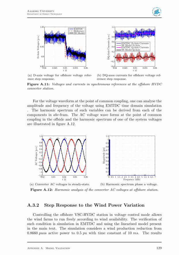
ii
“Thesis” — 2012/11/2 — 9:02 — page 129 — #129 ii
ii
ii
Aalborg UniversityDepartment of Energy Technology
0.04 0.045 0.05 0.055 0.060.85
0.9
0.95
1
1.05
t [s]
D-A
xisVoltages
[p.u.]
EMTDCReferenceSS Model
(a) D-axis voltage for offshore voltage refer-ence step response.
0.04 0.045 0.05 0.055 0.06−0.4
−0.2
0
0.2
0.4
0.6
0.8
1
1.2
t [s]
DQ-A
xisCurrents
[p.u.]
EMTDC D-Axis CurrentsSS Model D-AxisEMTDC Q-Axis CurrentsSS Model Q-Axis
(b) DQ-axes currents for offshore voltage ref-erence step response.
Figure A.11: Voltages and currents in synchronous references at the offshore HVDCconverter station.
For the voltage waveform at the point of common coupling, one can analyse theamplitude and frequency of the voltage using EMTDC time domain simulation. The harmonic spectrum of such variables can be derived from each of thecomponents in abc-fram. The AC voltage wave forms at the point of commoncoupling in the offside and the harmonic spectrum of one of the system voltagesare illustrated in figure A.12.
0.02 0.03 0.04 0.05 0.06−1.2
−1
−0.8
−0.6
−0.4
−0.2
0
0.2
0.4
0.6
0.8
1
1.2
t [s]
AC
Voltages
[p.u.]
vavbvc
(a) Converter AC voltages in steady-state.
0 0.5 1 1.5 2 2.5 3 3.5 4 4.5 5 5.5 6 6.5 70
0.1
0.2
0.3
0.4
0.5
0.6
0.7
0.8
0.9
1
1.1
Frequency [kHz]
Magnitude[pu]
(b) Harmonic spectrum phase a voltage.
Figure A.12: Harmonic analysis of the converter AC voltages at offshore station.
A.3.2 Step Response to the Wind Power Variation
Controlling the offshore VSC-HVDC station in voltage control mode allowsthe wind farms to run freely according to wind availability. The verification ofsuch condition is simulation in EMTDC and using the linearised model presentin the main text. The simulation considers a wind production reduction from0.8660 puos active power to 0.5 pu with time constant of 10 ms. The results
Appendix A. Model Validation 129

ii
“Thesis” — 2012/11/2 — 9:02 — page 130 — #130 ii
ii
ii
Aalborg UniversityDepartment of Energy Technology
showing the time domain comparison among the non-linear EMTDC model aswell as the state space model for the offshore side are presented in figure A.13.
0.04 0.05 0.06 0.07 0.08−0.2
0
0.2
0.4
0.6
0.8
1
1.2
t [s]
DQ-A
xisVoltages
[p.u.]
EMTDC D-Axis VoltagesSS Model D-AxisEMTDC Q-Axis VoltagesSS Model Q-AxisWPP Q
(a) Voltage at the PCC for the reduction inthe wind farm energy production
0.04 0.05 0.06 0.07 0.08−0.2
0
0.2
0.4
0.6
0.8
1
1.2
t [s]
DQ-A
xisCurrents
[p.u.]
EMTDC D−Axis CurrentsSS Model D−AxisEMTDC Q−Axis CurrentsSS Model Q−Axis
(b) Converter currents for the reduction in thewind farm energy production
Figure A.13: Simulation comparison between the EMTDC time domain simulationand the linearised state space model for wind power production variation.
A.3.3 Step Response to the Wind Power Reactive PowerCompensation
The weakness of the offshore grid is an important issue for controlling properlythe voltage at the point of common coupling. The wind farms, when consideringfull-scale converters as turbine conversion devices, are able to operate compensa-tion reactive power according to grid requirements. This action helps the offshoreconverter in maintaining the offshore grid voltage. For the modelling purpose, it isconsidered that the wind farms can fully support reactive power. The simulationcomparison between the EMTDC simulation platform and the state space modelof the offshore converter side considers constant wind production of 0.866 pu ofactive power and variation of wind farm reactive power from 0.1 pu to 0.3 pu atthe instant of time equal to 50 ms. This change is considered to be a step change.The results for such scenario is showed in figure A.14.
130 Appendix A. Model Validation

ii
“Thesis” — 2012/11/2 — 9:02 — page 131 — #131 ii
ii
ii
Aalborg UniversityDepartment of Energy Technology
0.04 0.05 0.06 0.07 0.08−0.2
0
0.2
0.4
0.6
0.8
1
1.2
t [s]
DQ-A
xisVoltages
[p.u.]
EMTDC D−AxisSS Model D−AxisEMTDC Q−AxisSS Model Q−AxisWPP Q
(a) Converter currents for the variation in thewind farm reactive power support
0.04 0.05 0.06 0.07 0.08−0.2
0
0.2
0.4
0.6
0.8
1
1.2
t [s]
DQ-A
xisCurrents
[p.u.]
EMTDC D-AxisSS Model D-AxisEMTDC Q-AxisSS Model Q-Axis
(b) Converter currents for the variation in thewind farm reactive power support
Figure A.14: Simulation comparison between the EMTDC time domain simulationand the linearised state space model for wind power reactive power compensation.
Appendix A. Model Validation 131

ii
“Thesis” — 2012/11/2 — 9:02 — page 132 — #132 ii
ii
ii
Aalborg UniversityDepartment of Energy Technology
132 Appendix A. Model Validation

ii
“Thesis” — 2012/11/2 — 9:02 — page 133 — #133 ii
ii
ii
APPENDIXBIntroduction to Optimal Robust
Control
B.1 Concepts
In layman’s terms, the robustness of the system from the figure 5.1 can bedefined as the amount of the variation of the parameter uncertainty and size ofthe disturbance and noise signals for which the system remains stable.
Stability is a crucial requirement in any feedback system. One can standin the need of certain performance level of the feedback system even whetherthe uncertainties and disturbances are included. By performance specificationthe criteria of settling time, damping factor, phase margin, rise time, maximumovershoot, are considered.
Usually, the controller C(s) is designed for the purpose of tracking the refer-ence signal, and, it is desired, that, on the same time, the effect of the parame-ter uncertainties, disturbance and measurement noise are attenuated. It is wellknown, however, that satisfying both sensitivity (output variation under effect ofthe parameter uncertainties, disturbance and noise) and reference tracking is aninfeasible problem [53].
So the performance specification of the system, e.g., tracking error, time re-sponse and maximum overshoot, can be satisfied for certain range of variation ofthe uncertainties and disturbances. By then, robust performance can be definedas the amount of variation of the uncertainties such that the system remains sta-ble and satisfy some of the performance criteria specified in the beginning of thecontrol design.
In optimal control theory, some techniques have been discussed in the litera-ture regarding using optimal controllers which have the optimal criteria based onthe minimisation of the impact of disturbances and uncertainties over the outputresponse [53, 54]. One of the tools presented by such theory is the µ-synthesis.
This technique aims to minimise the structured singular values of a dynamic
133

ii
“Thesis” — 2012/11/2 — 9:02 — page 134 — #134 ii
ii
ii
Aalborg UniversityDepartment of Energy Technology
system where the uncertainties are included in the model in a structured form.Details in this approach can be found in the references [53, 54, 51]. The followingsections describes, briefly the uncertainty modelling using the structured form aswell as the control synthesis. The method is then applied in the control of voltagesource converters as a possible control technique to reduce the sensitivity of thesystem under disturbance effects.
B.2 Uncertainty Model
The uncertainties in the system representation from figure 5.1 can be classifiedinto disturbance signals and dynamic perturbations [51]. The first case can beexemplified by changes in power and variation of the grid voltage and frequencyin a grid connected voltage source converter. The last case consider the disparitybetween the nominal model and the actual dynamics due to parameter variations.
Some of the uncertainties in the system that may occur can be grouped into onesingle perturbation block. For the present analysis, two main uncertainty typesare considered: the additive perturbation and inverse additive perturbation. Bothcases are illustrated in figure B.1.
K + δKInput Output
KInput Output
δK
(a) Additive
Input Output1K + δK
Input Output
δK
1K
(b) Incerse additive
Figure B.1: Additive and inverse additive uncertainty types.
Considering a general dynamic system M , and a set of parameters from Msuch that the uncertainties can be structured using the formulation in figure B.1,the standard configuration for representing the nominal system and its structureduncertainty block ∆ is represented in figure B.2.
where ∆ is a diagonal matrix such that, ∆ = diag δ1, δ2, . . . , δn, and δs are theuncertainties of the model.
The interconnection transfer function matrix M from figure B.2 can be frac-tionated such as (B.1).
M =
[M11 M12
M21 M22
](B.1)
It is defined as upper Linear Fraction Transformation (LFT) of M , the matrix
134 Appendix B. Introduction to Optimal Robust Control

ii
“Thesis” — 2012/11/2 — 9:02 — page 135 — #135 ii
ii
ii
Aalborg UniversityDepartment of Energy Technology
M(s)
Plant
Δ
Uncertainty Block
w z
Figure B.2: Standard representation of dynamic systems with structured uncertainties.
equation given by (B.2).
Fu(M,∆) =[M11 +M21∆ (I−M11∆)
−1M12
](B.2)
where I is the identity matrix.
As a generalisation of the concept of singular value decomposition, which canbe used for constant matrices, the structured singular values are able to deal withmatrices where the elements of the matrix can vary in a predefined range. Thedefinition of the calculation of structured singular values is written in figure (B.3).
µ∆ (M(s)) =1
min σ(∆) : det (I−M(s)) = 0, is structured (B.3)
The value of σ comes from the small gain theorem, briefly written in (B.4).
1
αmax:= ‖∆‖∞ = sup
s∈C+
σ (M(s)) = supωσ (M(jω)) (B.4)
The small gain theorem states that the maximum size of ∆, in terms of H∞-norm, is the supreme value of σ such that the feedback system remains marginallystable.
B.3 Control Synthesis and Performance
Considering the block diagram from figure 5.1, and the signals r(t), u(t), d(t)and y(t) as the reference signal, control signal, disturbance signal and the outputsignal, respectively, the relationship among them and the state space models fromthe block diagram are given by (B.5), (B.6) and (B.7)
y(t) = (I +GCHK)−1GCr(t) + (I +GCHK)
−1d(t) (B.5)
e(t) = HK (I +GCHK)−1
(HK)−1r(t)−HK (I +GCHK)
−1d(t) (B.6)
u(t) = GCHK (I +GCHK)−1
(HK)−1r(t)−GCHK (I +GCHK)
−1d(t)
(B.7)
Appendix B. Introduction to Optimal Robust Control 135

ii
“Thesis” — 2012/11/2 — 9:02 — page 136 — #136 ii
ii
ii
Aalborg UniversityDepartment of Energy Technology
The reference and disturbance signals are bounded, and considering the in-duced system norms of the blocks from figure 5.1, for the reference tracking, dis-turbance attenuation and less control energy, the minimisation of the H∞-normsare related respectively to:
Reference tracking:∥∥∥HK (I +GCHK)
−1∥∥∥∞
Disturbance attenuation:∥∥∥HK (I +GCHK)
−1∥∥∥∞
Control energy:∥∥∥GCHK (I +GCHK)
−1∥∥∥∞
As a standard procedure in optimal robust control, the sensitivity and com-plementary sensitivity functions can be defined by (B.8) and (B.9).
S :=Y (s)
D(s)(B.8)
T := 1−S (B.9)
Combining the equations (B.8), (B.9) with (B.5), (B.6) and (B.7), the sen-sitivity and complementary sensitivity functions from the block diagram fromfigure 5.1 can be written in (B.10) and (B.11).
S = (I +GCHK)−1
(B.10)
T = (I +GCHK)−1GCHK (B.11)
In accordance to (B.10) and (B.11) the seek for a stabilising controller can bewritten with regard to minimisation of the sensitivity function by (B.12).
minC Stabilising
∥∥∥HK (I +GCHK)−1∥∥∥∞
(B.12)
In general, the algorithms applied in the optimisation problem (B.12) havedifficulties for convergence [53]. By including weighting functions, the stabilisingcontroller to meet the design specifications can be, usually, found.
When the uncertainty block from figure B.2, which transfer matrix given bythe linear transformation (B.2), the problem can be translated by µ-synthesissolution problem using D-K Iteration.
Such optimisation problem is not convex and, as consequence, the global con-vergence is not guaranteed. The weighting design for such problem can alsorepresent a troublesome in the process design [55, 56]
B.4 D-K Iteration Algorithm
The µ-synthesis is a control methodology which tries to minimise the struc-tured values in a uncertain system by translating the problem in the definition of
136 Appendix B. Introduction to Optimal Robust Control

ii
“Thesis” — 2012/11/2 — 9:02 — page 137 — #137 ii
ii
ii
Aalborg UniversityDepartment of Energy Technology
system norms. Usually, the H∞ is used. The search for stabilising controllers ismade by a iterative method given by the D −K iteration.
Algorithm 4 D-K Iteration Algorithm
Require: Initialisation: initial controller K0(s)function 1. Closed Loop Function(Fl(P (s),K0(s)))
Calculation of the closed loop function between the plant P (s) and K0(s)end functionfunction 2. D-Scale(Upper Bounds)
Calculation of D scale using:infD(ω)
σmax[D(ω)Fl(P (jω),K0(jω))D−1(ω)
]
end functionfunction 3. Design(H∞)
Design H∞ for the system D(s)P (s)D−1(s)end function’Return to 1
Appendix B. Introduction to Optimal Robust Control 137

ii
“Thesis” — 2012/11/2 — 9:02 — page 138 — #138 ii
ii
ii
Aalborg UniversityDepartment of Energy Technology
138 Appendix B. Introduction to Optimal Robust Control

ii
“Thesis” — 2012/11/2 — 9:02 — page 139 — #139 ii
ii
ii
APPENDIXCPSCAD Model
The time domain simulation is built in PSCAD/EMTDC platform. The justi-fication for this choice lies on the fact that PSCAD is a well established simulationtool in the field of power systems. Basically, the model presents four main blocks:
1. Wind farm
2. Offshore HVDC station
3. DC cable
4. Onshore HVDC station
5. Onshore AC grid
The main diagram with the PSCAD modules are presented in figure C.1.
Wind FarmOffshore HVDC Station
CableOnshore HVDC Station
Grid
WPP Offshore Station Onshore Station Grid
Figure C.1: PSCAD main block diagram architecture.
139

ii
“Thesis” — 2012/11/2 — 9:02 — page 140 — #140 ii
ii
ii
Aalborg UniversityDepartment of Energy Technology
C.1 Wind Farm Model
The wind farm model contains the algebraic equation model for the calculationof currents based on the HVDC converter terminal voltages and the power order.The power model of the aggregated wind farm is, in PSCAD, modelled as currentsources. The circuit diagram is presented by figure C.2.
WPP Model:
a
b
c
ia
ib
icE
aE
bE
c100000.0 [ohm]
Figure C.2: PSCAD model for the aggregated wind power plant.
The nodes Ea, Eb and Ec are the voltage measurements. The labels ia, iband ic are the signals with the current signals.
The measurement of the voltages passes throughout the park transformation.The references for the currents are calculated using the instantaneous power the-ory. The input signals for the reference current calculation are the voltages andpower references. The first part of the current reference calculation containingthe measurement and reference frame transformation is presented in C.3.
*1
*-0.5
*-0.5
*-0.8660
*0.8660
*0
B+
D +
F
+
B+
D +
F
+
*0.8165
*0.8165
Clarke Transformation:
Grid AC Voltages:
valpha
vbeta
valpha *
Sin
Cos
vbeta*
B+
F
+
Park Transformation:
Direct Axis:
valpha *
Sin
Cos
vbeta*
B-
F
+
Quadrature Axis:
Ea
Eb
Ec
wt
wt
vd
vq
Synchronisation:
Synchronisation:
*0.00666666
*0.00666666
*0.00666666
[OffshoreVSCControl] Syn wt
Figure C.3: Wind power plant measurement and reference transformation.
The synchronisation signal is an external signal which comes from the offshoreHVDC station. The power calculation and inverse reference frame transformationis give by the by the figure C.4.
The external signals of power and reactive power commands are set duringthe simulation process. In the PSCAD model those signals are labelled with the
140 Appendix C. PSCAD Model
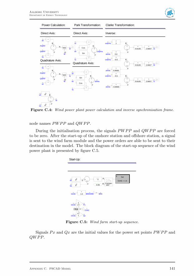
ii
“Thesis” — 2012/11/2 — 9:02 — page 141 — #141 ii
ii
ii
Aalborg UniversityDepartment of Energy Technology
Power Calculation:
Direct Axis:
X2vd
vq X2
B+
F
+ M
*vd
PWPP
QWPP
B+
F
-
*vq
*2.6667
Quadrature Axis:
N
D
N/D
M
*vq
PWPP
QWPP
B+
F
+
*vd
*2.6667
N
D
N/D
M
id
iq
*
Sin
Cos
*
B+
F
-
Park Transformation:
Direct Axis:
Quadrature Axis:
*
Sin
Cos
*
B+
F
+
ualpha
ubeta
Clarke Transformation:
Inverse:
*1
*0.0
*-0.8660
*-0.5
B+
F
+
B+
F
+
*0.8165
*0.8165
*0.8660
*-0.5 B
+
F
+*
0.8165
ualpha
ualpha
ualpha
ubeta
ubeta
ubeta
id
iq
id
iq
wt
wt*
2.6667
ia
ib
ic
Figure C.4: Wind power plant power calculation and inverse synchronisation frame.
node names PWPP and QWPP .
During the initialisation process, the signals PWPP and QWPP are forcedto be zero. After the start-up of the onshore station and offshore station, a signalis sent to the wind farm module and the power orders are able to be sent to theirdestination in the model. The block diagram of the start-up sequence of the windpower plant is presented by figure C.5.
Start-Up:
vd
vq
X2
X2
D +
F
+X A
B Compar-ator0.95
SetS
OnAC = 1.0
BRK*
1.0OnAC BRKKRB
Clear
1sTOnAC Px
Clear
1sT
OnAC Qx
OnAC
Figure C.5: Wind farm start-up sequence.
Signals Px and Qx are the initial values for the power set points PWPP andQWPP .
Appendix C. PSCAD Model 141

ii
“Thesis” — 2012/11/2 — 9:02 — page 142 — #142 ii
ii
ii
Aalborg UniversityDepartment of Energy Technology
C.2 Offshore Converter Station
The offshore converter station is composed by two main blocks: the convertercircuitry and the control module. The interconnected overview of the offshoremodules are presented in figure C.6.
Onshore Station Converter:
a
b
cVSC
VSC Control
100000.0 [ohm]
DCPx
DCNx
Figure C.6: Offshore PSCAD model with converter and control modules.
The AC side presents the nodes a, b and c which are connected to the windpower plant. The DC side nodes are connected by the DCPx and DCNx.
Inside the converter circuity module, the voltage source converter is built usingthe two-level topology. The main components are the converter phase reactor,switching devices, DC capacitor and high frequency filter which is included in aseparated block. The circuit schematic of the system is presented in figure C.7.
Power Circuit:
a
b
c
G
vCfa vCfb vCfc
II
I
D2D4D6
D1D3D5
VCo
II
II II
II
I
ILc
ILb
ILaIa
Ib
Ic
21.4859 [mH]
21.4859 [mH]
21.4859 [mH]
35.5
555
[uF]
DCN
DCP
ICo
35.5
555
[uF]
Figure C.7: Offshore converter circuit schematic.
The measurement points are indicated in figure C.7. The measurement vari-ables are grid currents, converter currents, DC voltages and filter voltages. Themeasurement signals are used for control purpose in the controller module. TheIGBT devices are controlled by means of PWM signals generated in the controlmodule. The signals related to the modulator are label with dn, where n is theswitch number.
The high frequency filter circuit diagram is presented in figure C.8.
142 Appendix C. PSCAD Model

ii
“Thesis” — 2012/11/2 — 9:02 — page 143 — #143 ii
ii
ii
Aalborg UniversityDepartment of Energy Technology
VCfcVCfbVCfa
a b c
AC Filter:
G
28.8462 [ohm]
470.8726 [uH]14.1471 [uF]
28.8462 [ohm]
470.8726 [uH]14.1471 [uF]
28.8462 [ohm]
470.8726 [uH]14.1471 [uF]
Figure C.8: Circuit schematic for the high frequency filter.
The control module is composed by five main modules: the measurementswith the feedback gains, the synchronous reference frame transformation, thecontrollers including PLL (disabled in the offshore station), current controller andAC voltage controller, the inverse reference transformation and the modulator.The five blocks are in the schematic presented by figure C.9.
Measurements:
Grid Voltages:
vCf
*0.00666666
123
*0.00666666
*0.00666666
vavbvc
Controllers:
PLL:
va
vb
vc
w
o
Converter Currents:
iL
*0.37500
123
iLaiLbiLc
*0.37500
*0.37500
Reference Transformation:
Park:
va
vb
vc
iLa
iLb
iLc
o
vd
vq
id
iq
Reference Transformation:
Park:
Current Controller
id
iq
ud
uq
Enable
iqx
DQ0_
ud
uq
o
Modulation:
Modulation:
ua
ub
uc
PWM
ua
ub
uc
Enable
123
PWM
vd
vq
w
vCo
DC Voltage:
*3.3333e-3 vBus
vBus
iCo *0.7500 iBus
idx
vBus
po*
314.1593
PLL
CC
Enable
Grid Currents:
i
*0.37500
123
iaibic
*0.37500
ia
ib
ic
DQ0Do
iGD
iGQ
*0.37500
Voltage Controller
idx
iqxvq
Syn
AC
Enable
REF
vd
0.0
Figure C.9: Offshore control block diagram.
The measurement column includes the feedback of the VSC circuit. The vari-ables are scaled by block gains. The next stage in the control flow chart is thesynchronous reference transformation. The variables in the abc domains are trans-formed to the φdq-frame by means of a linear transformation. The matrix formatof given in the main text. In PSCAD, the calculation is made by means of theschematic presented in figure C.10.
Appendix C. PSCAD Model 143

ii
“Thesis” — 2012/11/2 — 9:02 — page 144 — #144 ii
ii
ii
Aalborg UniversityDepartment of Energy Technology
*1
*-0.5
*-0.5
*-0.8660
*0.8660
*0
B+
D +
F
+
B+
D +
F
+
*0.8165
*0.8165
Clarke Transformation:
Grid AC Voltages:
va
vb
vco
valpha
vbeta
valpha *
Sin
Cos
vbeta*
B+
F
+
Park Transformation:
Direct Axis:
vqo
valpha *
Sin
Cos
vbeta*
B-
F
+
Quadrature Axis:
*1
*-0.5
*-0.5
*-0.8660
*0.8660
*0
B+
D +
F
+
B+
D +
F
+
*0.8165
*0.8165
Grid AC Currents:
iLa
iLb
iLciLdo
iLalpha
iLbeta
iLalpha *
Sin
Cos
iLbeta*
Direct Axis:
iLqo
iLalpha *
Sin
Cos
iLbeta*
Quadrature Axis:
vd
B-
F
+
B+
F
+
*1
*-0.5
*-0.5
*-0.8660
*0.8660
*0
B+
D +
F
+
B+
D +
F
+
*0.8165
*0.8165
Grid AC Currents:
ia
ib
icido
ialpha
ibeta
ialpha *
Sin
Cos
ibeta*
Direct Axis:
iqo
ialpha *
Sin
Cos
ibeta*
Quadrature Axis:
B-
F
+
B+
F
+
Figure C.10: Park transformation implemented in PSCAD simulation platform.
The current controller is the following block in the process. Its main structureis formed by error calculation, PI control with unitary gain, the augmented controlblock and the feedforwards (decoupling, AC and DC voltages). The PSCADdiagram for the current controller is illustrated in figure C.11.
The central block in the figure C.11 is the implementation of a state spacemodel in C code. During the simulations this block can be changed to a static
144 Appendix C. PSCAD Model

ii
“Thesis” — 2012/11/2 — 9:02 — page 145 — #145 ii
ii
ii
Aalborg UniversityDepartment of Energy Technology
Current Controllers:
Direct Axis:
idx
Ena
ble
Quadrature Axis:
iqx
Enable
ud
uq
vd
D -
F+
D -
F
+
A
BCtrl
Ctrl = 1
0.0 Enable
A
BCtrl
Ctrl = 1
0.0 Enable
iq
w
*0.
0177
7777
8
D +
F
+
vBus
D +
F- D +
F+
vq vBus
N
D
N/D
*0.
0177
7777
8
id
w
Clear
1sT
Clear
1sT
N
D
N/D
id
iq
D +
F
+
eDeQ
Control: PI and Feedforward:
*0.0214859
*0.0214859
*
*
udPI
uqPI
In Out
x
1 2 3 4
VSCOnshoremuDQ.c
12
Figure C.11: PSCAD implementation of the current controller.
gain, in case of the PI selection control mode, or using the robust controller.For the initialisation purpose, the integrators are not operating. After the a flagindication for normal operation all the integrator are de-blocked.
For the AC voltage controllers, the error signal comparison, unitary PIs andthe high order controllers are presented. The high order controller is, again, im-plemented in a external C function. For th AC voltage controller, the figure C.12illustrates the implementation in PSCAD of the AC voltage controller for theoffshore station.
Voltage Controllers:
Direct Axis:
Quadrature Axis:
D -
F
+A
BCtrl
Ctrl = 1
0.0
Clear
1sT
Enable
vDi
vD
uD
D -
F
+A
BCtrl
Ctrl = 1
0.0
Clear
1sT
vQi
vQ
uQ
Enable
In Out
x
1 2 3 4
jRobustACOffshore.c
1
2
Figure C.12: PSCAD implementation of the AC voltage controller.
The inverse reference transformation generates the sinusoidal waveforms which
Appendix C. PSCAD Model 145

ii
“Thesis” — 2012/11/2 — 9:02 — page 146 — #146 ii
ii
ii
Aalborg UniversityDepartment of Energy Technology
are going to be compared with the triangular carrier in the modulator. ThePSCAD implementation of the inverse synchronous reference frame transforma-tion is illustrated in figure C.13.
o
*
Sin
Cos
*
B+
F
-
Park Transformation:
Direct Axis:
Quadrature Axis:
ud
uq
o
*
Sin
Cos
*
B+
F
+
ud
uq
ualpha
ubeta
Clarke Transformation:
Inverse:
*1
*0.0
*-0.8660
*-0.5
B+
F
+
B+
F
+
*0.8165
*0.8165
*0.8660
*-0.5 B
+
F
+*
0.8165
ualpha
ualpha
ualpha
ubeta
ubeta
ubeta
ua
ub
uc
Figure C.13: Inverse Park transformation implemented in PSCAD simulation plat-form.
After the inverse Park’s Transformation, the sinusoidal signals are comparedwith the triangular carrier. This comparison generates the PWM signals whichare injected in the IGBT drives in the power circuit. The PSCAD model for themodulator is illustrated in figure C.14.
Modulation:
A
B Compar-ator
A
BCtrl
Ctrl = 1
0.0
Carrier
Enable
PWMa
Phase a:
A
B Compar-ator
A
BCtrl
Ctrl = 1
0.0
Carrier
Enable
PWMb
Phase b:
A
BCtrl
Ctrl = 1
0.0
Carrier
Enable
PWMc
Phase c:
Carrier:
Carrier
ua
ub
uc A
B Compar-ator
Figure C.14: Modulation PSCAD implementation schematic.
146 Appendix C. PSCAD Model

ii
“Thesis” — 2012/11/2 — 9:02 — page 147 — #147 ii
ii
ii
Aalborg UniversityDepartment of Energy Technology
The start-up of the offshore station is based in the measurement of the DCvoltage presented in the DC link. It is set by assumption that, after the DC voltageachieves more than 97% of the nominal DC voltage, the rest of the controllers areenabled. The start block sequence and commands are shown in figure C.15.
Enable
Start
Start-Up:
Main Breaker:
Offs...Main Breake...
0
ON OFF
Inrush Breakers:
vd
vq
X2
X2
D +
F
+X A
B Compar-ator0.95
SetS
OnAC = 1.0
A
B Compar-ator
0.97
5
SetS
OnDC = 1.0
123
StartOnDC
BRK
vBus 10 [ms]
Wait UntilS
1sTEnable REFx
1.0
*1.0OnDC
Figure C.15: Offshore station start-up sequence implementation.
The signal REFx is the initial value for the AC voltage reference. The in-tegrator generates the ramp signal for the initialisation of the voltage reference.The start-up of the offshore station can be also controlled by the manual controlswitch from PSCAD blockset.
Appendix C. PSCAD Model 147

ii
“Thesis” — 2012/11/2 — 9:02 — page 148 — #148 ii
ii
ii
Aalborg UniversityDepartment of Energy Technology
C.3 Onshore Converter Station
The offshore station has approximately the same structure presented by theoffshore station. The main modules, the converter circuit module and the controlmodules are in the same way connected as in the figure C.6. The onshore convertercircuit has, however, fewer components added in order to provide the properinitialisation. The figure C.16 shows the circuit diagram of the onshore converterstation.
Power Circuit:
a
b
c
G
vCfavCfbvCfc
I I
I
D2 D4 D6
D1 D3 D5
VCo
I I
I II I
I I
I
ILc
ILb
ILa Ia
Ib
Ic
BRK2
BRK2
BRK2
21.4859 [mH]
56.25 [ohm]
56.25 [ohm]
56.25 [ohm]
21.4859 [mH]
21.4859 [mH]
BRK1
BRK1
BRK1
35.5555 [uF]35.5555 [uF]
ICo
DCP
DCN
Figure C.16: Onshore converter circuit schematic.
From figure C.16, it is possible to observe the presence of two breaker in themain circuit. They are included to the operation of the converter during the start-up.After the main breaker (BRK1) be enabled, the in-rush currents are limited bythe series resistors connected in parallel with the in-rush breaker (BRK2). Aftera control command be send, the in-rush breaker is enabled and the system cango to the normal operation. The rest of the components of the onshore convertercircuitry are the same as presented for the offshore converter station.
Compared with the offshore station, the onshore converter control has twomain differences. The first off is that the controller is connected to the grid utilityand must be in synchronisation with the other generators. For this purpose,the phase-lock loop is included in the control architecture. The block diagramrepresentation of the PLL implemented in PSCAD is given in the figure C.17.
Due to the control operation mode the onshore converter is enabled to regulatethe DC voltage across the DC capacitor. As mentioned in the main text, the DCvoltage is measured and squared for the compensation of the energy balance inthe DC capacitor. The reference signal is provided by the station operator and itsvalue is compared with the measured values squared. This error is compensated,firstly, by the proportional integral controller and after that by the robust con-troller, if enabled. The current reference signal is then generated after the controlcompensation.
148 Appendix C. PSCAD Model

ii
“Thesis” — 2012/11/2 — 9:02 — page 149 — #149 ii
ii
ii
Aalborg UniversityDepartment of Energy Technology
Clarke Transformation:
*1
*-0.5
*-0.5
*-0.8660
*0.8660
*0
B+
D +
F
+
B+
D +
F
+
*0.8165
*0.8165
*
Sin
B-
F
+
a
b
cwo
w
D +
F
+
Cos
o
alpha
Clear
1sT
A
BCompar-ator 3.14159265359
beta *
Controller: Oscilator:
*111.07207B
+
F
+1
sT
Phase Detector:
Figure C.17: Phase-lock loop implementation is PSCAD platform.
The implementation in PSCAD follows this procedure. The error generationand PI controller are directly extracted from the default PSCAD blocks. Therobust controller is implemented suing C function using the same approach whichwas developed for the current and AC voltage controllers. The PSCAD blockdiagram of the DC voltage controller is illustrated in figure
DC Voltage Controller:
Control:
uDC
RobustDCOnshore.c
In Out
x
D +
F
-A
BCtrl
Ctrl = 1
Clear
1sT
vDCx
vDCo
Ena
ble
0.0
X2
0.1
A
BCtrl
Ctrl = 1
Figure C.18: PSCAD implementation of the DC voltage controller.
The start-up sequence of the onshore converter is performed by the control ofthe operation of the circuit breakers included in the power circuit. First of all,the measurements of the AC voltage initiates the sequence. The main breaker isactivated (BRK1) and after the DC voltages achieves 60% of its nominal valuethe inrush breaker is enabled. The current controller is then activated and the Dcvoltage at the DC link is boosted up to its nominal value. After this point, theDC voltage controller is enabled and the converter is under normal operation.
The block diagram showing the flags and measurable variable for the start-upof the onshore HVDC converter is illustrated by the diagram in figure C.19.
Appendix C. PSCAD Model 149

ii
“Thesis” — 2012/11/2 — 9:02 — page 150 — #150 ii
ii
ii
Aalborg UniversityDepartment of Energy Technology
Enable
Start
Main Breaker:
: Co...<null>
Inrush Breakers:
vd
vq
X2
X2
D +
F
+X A
B Compar-ator0.95
SetS
OnAC = 1.0
A
B Compar-ator
0.6
SetS
OnDC = 1.0
OnACOnDC
Start SetS
Boost = 1.0
A
B Compar-ator
0.98
SetS
On = 1.0
123
StartOnDC
On
BRK
vBus
vBus
10 [ms]
Wait UntilS
Start-Up:
Figure C.19: Onshrore start-up sequence implementation in PSCAD.
150 Appendix C. PSCAD Model