aalborg universitet probabilistic analysis methods for
TRANSCRIPT

Aalborg Universitet
Probabilistic analysis methods for support structures
Work Package - D7.42
Gintautas, Tomas; Sørensen, John Dalsgaard; Natarajan, Anand; Wandji, Wilfried Njomo;Dimitrov, Nikolay Krasimirov; Ehrmann, Andreas; Hübler, Clemens; Schmoor, Kirill; Pfaffel,Sebastian; Faulstich, Stefan
Creative Commons LicenseUnspecified
Publication date:2018
Document VersionPublisher's PDF, also known as Version of record
Link to publication from Aalborg University
Citation for published version (APA):Gintautas, T., Sørensen, J. D., Natarajan, A., Wandji, W. N., Dimitrov, N. K., Ehrmann, A., Hübler, C., Schmoor,K., Pfaffel, S., & Faulstich, S. (2018). Probabilistic analysis methods for support structures: Work Package -D7.42 . European Commission * Office for Official Publications of the European Union.
General rightsCopyright and moral rights for the publications made accessible in the public portal are retained by the authors and/or other copyright ownersand it is a condition of accessing publications that users recognise and abide by the legal requirements associated with these rights.
? Users may download and print one copy of any publication from the public portal for the purpose of private study or research. ? You may not further distribute the material or use it for any profit-making activity or commercial gain ? You may freely distribute the URL identifying the publication in the public portal ?
Take down policyIf you believe that this document breaches copyright please contact us at [email protected] providing details, and we will remove access tothe work immediately and investigate your claim.
Downloaded from vbn.aau.dk on: December 29, 2021

Integrated Research Programme on Wind Energy
Project acronym: IRPWIND
Grant agreement no 609795
Collaborative project
Start date: 01st December 2013
Duration: 4 years
Probabilistic analysis methods for support structures
Work Package – D7.42
Lead Beneficiary:
Delivery date:
Dissemination level: PU
The research leading to these results has received funding
from the European Union Seventh Framework Programme
under the agreement 609795.

IRPWIND deliverable - project no. 609795
2
Author(s) information (alphabetical):
Name Organisation Email
Tomas Gintautas AAU [email protected]
John Dalsgaard Sørensen AAU [email protected]
Anand NatarajanWilfried
N. Wandji
DTU Wind Energy [email protected]
Nikolay Dimitrov DTU Wind Energy
Andreas Ehrmann ForWind-Hannover [email protected]
Clemens Hübler ForWind-Hannover [email protected]
Kirill Schmoor ForWind-Hannover [email protected]
Sebastian Pfaffel Fraunhofer IEE [email protected]
Stefan Faulstich Fraunhofer IEE [email protected]
Acknowledgements/Contributions:
Name Name Name
Document Information Version Date Description
1 28/02/2018 Initial Version
Prepared by Reviewed by Approved by
Name Kim Branner All All
Definitions
IRPWIND deliverable - project no. 609795
3
Table of Contents
Integrated Research Programme on Wind Energy ................................................................ 1
Probabilistic analysis methods for support structures .......................................................... 1
Work Package – D7.42............................................................................................................ 1
Executive Summary: ................................................................................................................ 1
1. Reliability Assessment of conical grouted joint ............................................................. 3
1.1 Introduction ................................................................................................................... 3
1.2 Bolted Joints .................................................................................................................. 4
1.3 Estimation of stress concentration factors at Welded Joints ..................................... 5
1.3.1. Strength limit state .......................................................................................... 6
1.4 Metocean conditions ..................................................................................................... 7
1.5 Finite Element Modeling of the Grouted Joint ............................................................. 9
1.6 Limit states for the conical grouted joint design ...................................................... 10
1.6.1 Limit states related to extreme events .............................................................. 10
1.6.2 Limit states related to fatigue ............................................................................ 10
1.7 Design for Fatigue of the Grouted Joint .................................................................... 11
1.7.1 Vertical settlement .............................................................................................. 13
1.8 Design for Extremes ................................................................................................... 15
1.8.1. Dimensionality reduction and parametrization................................................ 15
1.8.2 Simulation of Extreme Response of Grouted Joint ........................................... 18
1.8.3 Prediction of the extreme settlement ................................................................ 20
2. Reliability assessment of grouted joint with shear keys ............................................ 22
2.1 Target reliability levels .......................................................................................... 22
2.1 Deterministic assessment of concrete grout fatigue resistance ....................... 23
2.1.1 Deterministic assessment according to DNVGL-ST-C502.......................... 23
2.1.2 Deterministic assessment according to fib Model Code 2010 ................. 24
2.2 Reliability assessment of grouted joint – Concrete grout fatigue ..................... 27
2.2.1 Stochastic model for concrete grout fatigue ............................................... 28
2.2.2 Results of concrete grout reliability analysis............................................... 30
2.3 Reliability assessment of grouted joint – fatigue of welded steel details ......... 34
2.3.1 Stochastic model for steel fatigue ............................................................... 34
2.3.2 Results steel fatigue reliability analysis ...................................................... 38
2.4 Concluding remarks on reliability of tubular grouted connection with shear keys
41
3. Reliability of piles and substructures under consideration of soil parameters ........ 42
3.1 Reliability of the substructure under consideration of the turbine and soil
parameters ........................................................................................................................ 42
3.1.1 Introduction ................................................................................................... 43
3.1.2 Determination of the model error ................................................................ 44
3.1.2.1 Design methods ........................................................................................ 44
3.1.2.2 Calculated tension capacity of tested piles ............................................ 45
3.1.2.3 Derivation of the model error ................................................................... 46
3.1.3 Assesment of design methods ..................................................................... 52
3.1.3.1 Pile-Soil System under consideration ...................................................... 52
3.1.3.2 Deterministic design ................................................................................. 53
3.1.3.3 Stochastic soil model ................................................................................ 55
3.1.3.4 Reliability based design ............................................................................ 58
3.1.3.5 Comparison of deterministic and reliability based design ..................... 59
3.1.3.6 Evaluation of design methods .................................................................. 60

IRPWIND deliverable - project no. 609795
4
3.1.4 Summary and Conclusion ............................................................................. 62
3.2 Reliability of the substructure under consideration of the turbine and soil
parameters ........................................................................................................................ 64
3.2.1 Introduction and concept ............................................................................. 64
3.2.2 Wind turbine model....................................................................................... 65
3.2.2.1 Time domain model .................................................................................. 65
3.2.2.2 Soil model for transient calculations ....................................................... 66
3.2.2.3 Assessment of basic soil models with data from WP7.2 ....................... 76
3.2.3 Statistical distributions of input parameters............................................... 83
3.2.4 Sensitivity analysis ........................................................................................ 86
3.2.5 Deterministic and probabilistic design ........................................................ 89
3.2.6 Damage distribution and failure probabilities ............................................ 91
3.2.7 Summary and conclusion ............................................................................. 94
4. Failure statistics and current reliability level (Fraunhofer IEE) .................................. 95
4.1 Design and System Boundary of Support Structures (Fraunhofer IEE) ............. 96
4.2 Failure Modes of Support Structures (Fraunhofer IEE) ...................................... 97
5. References .................................................................................................................... 99
LEANWIND deliverable - project no. 614020
1
Executive Summary:
This report describes aspects of probabilistic analysis for offshore substructures and the
results obtained in various illustrative investigations. This includes probabilistic modeling
of model uncertainties using results from WP7.2 and WP7.3 on experimental data and
conventional design approaches.
Since no failures / collapses of wind turbine support structures are reported in the
literature / available databases statistical analyses have not been performed to assess
the reliability level. However, failures of the grouting in a large number of grouted
monopiles have been observed. These failures which can be considered as design errors
/ lack of knowledge seem only to have resulted in local failures without collapse of the
substructures, but have required various mitigation efforts incl. extensive inspection and
monitoring programs. For new designs the problem with groutings has resulted in changed
designs with e.g. shear keys or conical joints. The target reliability level in the design
standards for substructures corresponds to an annual probability of failure equal to
approximately 10-4 – 5 10-5.
Reliability analysis of offshore support structures can be performed using structural
reliability methods implying formulation of limit state equations for the critical failure
modes due to extreme loads and fatigue, and establishment of stochastic models for the
uncertain parameters in the limit state equations incl. physcial, statistical and model
uncertainties. The probability of failure can be estimated by simulation techniques or
First/Second Order Reliability Methods.
For the grouted joints a number of limit state equations are formulated related to critical
failure modes, including failure of the grout concrete in extreme loading and fatigue, and
fatigue failure for the welded steel details. Additionally, stochastic models are established.
Reliability analyses are performed using the limit states and illustrated for the 10 MW
reference wind turbine substructure for which load effects are obtained for extreme loads,
and combined stress ranges and mean stresses are obtained for fatigue analyses using a
detailed finite element modelling of the grouted connection.
For extreme loading failure of the concrete in shear and compression is investigated as
well as critical vertical settlement. Further, failure of the concrete in fatigue is considered.
Among others, the results show that the reliability level is sufficient related to settlement
of transition piece keeping the gap between the pile top edge and the jacking brackets
below 72 mm.
Fatigue reliability of concrete grout and steel components of grouted connection with
shear keys was assessed and found to be satisfactory at this stage of preliminary design.
The results show that the concrete grout reliability models are highly sensitive to model
errors related to the estimation of the SN curve, especially for the ‘compression to tension’
case where more test data are required. The reliability analyses of fatigue failure of the
welded steel details show a satisfactory reliability level, assuming cathodic protection
during the whole lifetime but also high sensitivity to assessment of the load stress ranges
IRPWIND deliverable - project no. 609795
2
and stress concentration/magnification factor calculations. Additionally, the results show
that for welds in both the monopile and transition piece larger initial cracks could be
allowed potentially reducing the manufacturing costs of monopiles and transition pieces.
For the geotechnical reliability assessment of foundation piles typical offshore soil and
foundation pile properties for offshore wind converters in the North Sea were assumed.
Five different design methods for the determination of the axial tensile resistance were
considered, and 60 deterministic designs were evaluated within a reliability based design.
Typical variability for the assumed soil condition and estimated model uncertainties were
applied for a reliability based estimation of failure probabilities in terms of reliability
indices. A new calibration approach was developed to determine the global safety factor
for a prescribed acceptable failure probability. Further, quality factors were derived for
each design method as function of the load, pile diameter, and soil density.
Nest, probabilistic calculations of fully coupled offshore wind turbines were considered in
order to assess the reliability of substructures, based on sophisticated, non-linear aero-
elastic simulations, and furthermore, to create the basis for safety factor (SF) calibration
It can be concluded that SFs can be reduced if probabilistic calculations are performed
implying possible weight saving potentials. The results also include global sensitivity
analyses whereby the most influential probabilistic parameters were identified showing
that wind and wave, and some soil parameters, have to be modelled by probabilistic
models.
IRPWIND deliverable - project no. 609795
3
1. Reliability Assessment of conical grouted joint
1.1 Introduction
Offshore wind turbine support structures for wind turbines typically possess welded,
bolted, or grouted joints. Most joints in the tower and substructure (monopile, jacket) are
usually welded joints. For monopiles, the connection between the cylindrical pile and the
tower is conventionally made using a grouted joint (Dallyn, et al., 2015). The tower
sections can also have bolted sections, typically ring flange connections that link different
sections of the tower together. The grouts at the transition between tower and monopile
may often be the weakest link in the overall support structure due to the action of the
cyclic loading from the wind turbine on the concrete material in the grout (Schaumann, et
al., 2013).
The fatigue design of grouted joints is influenced mainly by crushing and cracking of the
concrete grout layer, especially under tensile cyclic stresses common in wind turbine
operation. If this joint is instead made into a bolted joint, then several bolts are needed
along the circumference of two flanged intersections connecting the tower and monopile
(Madsen, et al., 2017). Classically, the grouted joints for monopile substructures are built
from the overlap of two cylindrical tubes: a transition piece and a pile, and the resulting
annular gap is filled with a high strength concrete. The grouted joints are efficient as they
are easily constructible and they serve to correct the pile misalignment due to driving
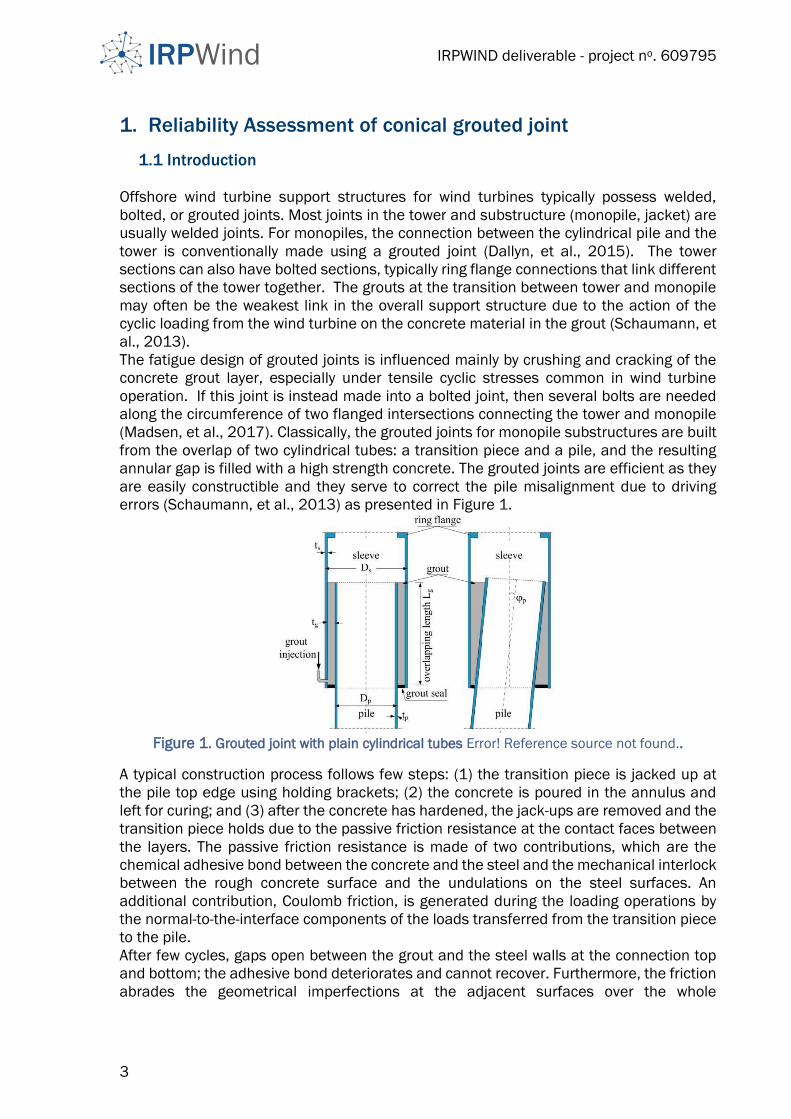
errors (Schaumann, et al., 2013) as presented in Figure 1.
Figure 1. Grouted joint with plain cylindrical tubes Error! Reference source not found..
A typical construction process follows few steps: (1) the transition piece is jacked up at
the pile top edge using holding brackets; (2) the concrete is poured in the annulus and
left for curing; and (3) after the concrete has hardened, the jack-ups are removed and the
transition piece holds due to the passive friction resistance at the contact faces between
the layers. The passive friction resistance is made of two contributions, which are the
chemical adhesive bond between the concrete and the steel and the mechanical interlock
between the rough concrete surface and the undulations on the steel surfaces. An
additional contribution, Coulomb friction, is generated during the loading operations by
the normal-to-the-interface components of the loads transferred from the transition piece
to the pile.
After few cycles, gaps open between the grout and the steel walls at the connection top
and bottom; the adhesive bond deteriorates and cannot recover. Furthermore, the friction
abrades the geometrical imperfections at the adjacent surfaces over the whole
IRPWIND deliverable - project no. 609795
4
connection length. At very early age of the structure, the two initial contributions
depreciate and only the coulomb friction persists, which is only effective when the normal
pressure is present. In case of insignificant normal pressure, the shear resistance may
not support the structure weight anymore and the transition piece will progressively slide
downwards till the jacking brackets touch the pile top edge: the connection fails.
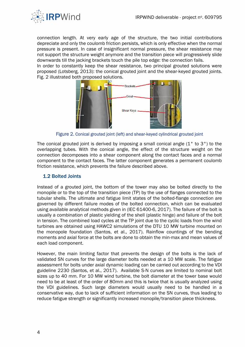
In order to constantly keep the shear resistance, two principal grouted solutions were
proposed (Lotsberg, 2013): the conical grouted joint and the shear-keyed grouted joints.
Fig. 2 illustrated both proposed solutions.
Figure 2. Conical grouted joint (left) and shear-keyed cylindrical grouted joint
The conical grouted joint is derived by imposing a small conical angle (1° to 3°) to the
overlapping tubes. With the conical angle, the effect of the structure weight on the
connection decomposes into a shear component along the contact faces and a normal
component to the contact faces. The latter component generates a permanent coulomb
friction resistance, which prevents the failure described above.
1.2 Bolted Joints
Instead of a grouted joint, the bottom of the tower may also be bolted directly to the
monopile or to the top of the transition piece (TP) by the use of flanges connected to the
tubular shells. The ultimate and fatigue limit states of the bolted-flange connection are
governed by different failure modes of the bolted connection, which can be evaluated
using available analytical methods given in (IEC 61400-6, 2017). The failure of the bolt is
usually a combination of plastic yielding of the shell (plastic hinge) and failure of the bolt
in tension. The combined load cycles at the TP joint due to the cyclic loads from the wind
turbines are obtained using HAWC2 simulations of the DTU 10 MW turbine mounted on
the monopole foundation (Santos, et al., 2017). Rainflow countings of the bending
moments and axial force at the bolts are done to obtain the min-max and mean values of
each load component.
However, the main limiting factor that prevents the design of the bolts is the lack of
validated SN curves for the large diameter bolts needed at a 10 MW scale. The fatigue
assessment for bolts under axial dynamic loading can be carried out according to the VDI
guideline 2230 (Santos, et al., 2017). Available S-N curves are limited to nominal bolt
sizes up to 40 mm. For 10 MW wind turbine, the bolt diameter at the tower base would
need to be at least of the order of 80mm and this is twice that is usually analyzed using
the VDI guidelines. Such large diameters would usually need to be handled in a
conservative way, due to lack of sufficient information on the SN curves, thus leading to
reduce fatigue strength or significantly increased monopile/transition piece thickness.
IRPWIND deliverable - project no. 609795
5
The effects of stress concentration factors/notch factors at the bolts, plastic yielding
conditions and the uncertain SN curves leads to a high uncertainty of bolted connections
for large offshore monopiles. The SN curve scaling or analysis of fatigue as a function of
the component size can be made with advanced FE models along with material tests, but
this is not feasible within the scope of this deliverable. Therefore this solution is not
considered further herein.
1.3 Estimation of stress concentration factors at Welded Joints The monopile, grout and transition piece have several welded connections between
cylindrical sections. The hotspot at the welds stresses are evaluated using stress
concentration factors (SCFs) at the weld connections. The weld connections of the
appurtenances to the main steel are not studied here. For butt connections with same
nominal diameter and thickness, (DNV-RP-C203, 2011) recommends estimating SCFs as
in Equation (1):
𝑆𝐶𝐹 = 1 +3 𝛿𝑚𝑡
𝑒−√𝑡/𝐷 (1)
where 𝐷 and 𝑡 are respectively the outer diameter and the wall thickness, 𝛿𝑚 = √𝛿𝑡2 + 𝛿𝑟2
is the resultant geometric imperfection measure, whose components are due to out-of-
roundness or eccentricity. The actual imperfection measure is project dependent and
brings uncertainties to the design procedure as it cannot accurately be predicted in
advance. Imperfection levels, 𝜆 , can be defined as the ratios between the resultant
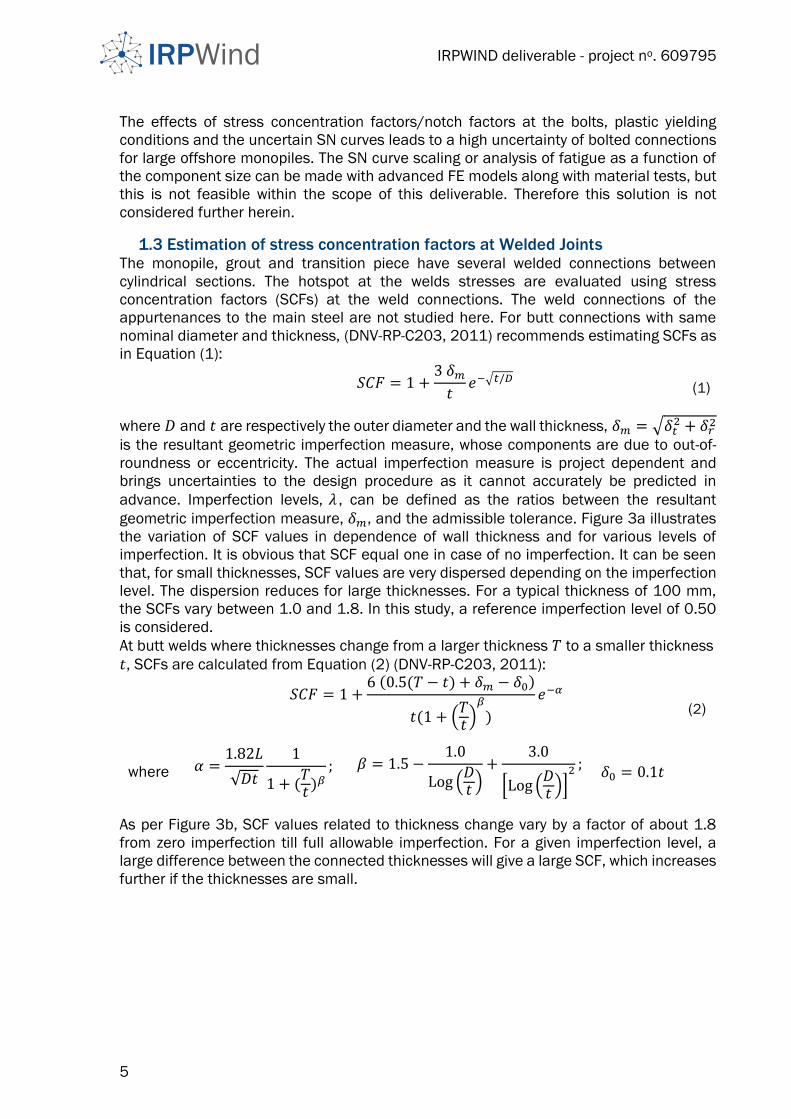
geometric imperfection measure, 𝛿𝑚, and the admissible tolerance. Figure 3a illustrates
the variation of SCF values in dependence of wall thickness and for various levels of
imperfection. It is obvious that SCF equal one in case of no imperfection. It can be seen
that, for small thicknesses, SCF values are very dispersed depending on the imperfection
level. The dispersion reduces for large thicknesses. For a typical thickness of 100 mm,
the SCFs vary between 1.0 and 1.8. In this study, a reference imperfection level of 0.50
is considered.
At butt welds where thicknesses change from a larger thickness 𝑇 to a smaller thickness
𝑡, SCFs are calculated from Equation (2) (DNV-RP-C203, 2011):
𝑆𝐶𝐹 = 1 +
6 (0.5(𝑇 − 𝑡) + 𝛿𝑚 − 𝛿0)
𝑡(1 + (𝑇𝑡)
𝛽
)
𝑒−𝛼 (2)
where 𝛼 =1.82𝐿
√𝐷𝑡
1
1 + (𝑇𝑡)𝛽; 𝛽 = 1.5 −
1.0
Log (𝐷𝑡 )+
3.0
[Log (𝐷𝑡 )]
2 ; 𝛿0 = 0.1𝑡
As per Figure 3b, SCF values related to thickness change vary by a factor of about 1.8
from zero imperfection till full allowable imperfection. For a given imperfection level, a
large difference between the connected thicknesses will give a large SCF, which increases
further if the thicknesses are small.
IRPWIND deliverable - project no. 609795
6
Figure 3. Effect of the geometry imperfection on stress concentration factors for a) butt welds
with same thickness and b) butt welds with varying thickness.
Thus at the transition piece near the grouted joint, the welded connections can have large
thickness thus supporting a large part of the load, but with small change in thickness
between successive vertical sections. This will enable a low uncertainty in fatigue damage
from stress concentration factors from the welded joints at the grouted connection.
1.3.1. Strength limit state
The steel strength and the pile stability are dependent on steel material properties, which
are given in Table 1.
Table 1: Steel properties of the monopile’s material.
Properties References Values
Steel type DNV-OS-J101 High strength steel (HS) / NV-32
Minimum yield stress [MPa] DNV-OS-J101 315
Mass density [kg/m3] Cremer and Heckl 7850
Effective Elastic Modulus [GPa] Cremer and Heckl 210
Poisson’s ratio [-] Cremer and Heckl 0.3
The main stress components at the transition piece are the longitudinal membrane stress,
the shear stress, and the circumferential membrane stress (see Figure 4).

IRPWIND deliverable - project no. 609795
7
Figure 4. Primary resulting stresses applied on a monopile shell.
The longitudinal membrane stress and the shear stress are given by Equations (3) and
(4), respectively:
𝜎𝑥 =𝑁
𝐴+𝑀1𝐼/𝑅
sin 𝜃 −𝑀2
𝐼/𝑅cos 𝜃 (3)
𝜏 = |𝑇
2𝜋𝑡𝑅2−2𝑄1𝐴sin 𝜃 +
2𝑄2𝐴cos 𝜃| (4)
The circumferential membrane stress is expressed as:
𝜎𝛼 =𝑝(𝑦)
4𝜋𝑡[4 − (𝜋 − 2𝛼)sin𝛼] (5)
where
𝑁 : axial force
𝑀1, 𝑀2 : bending moments about axis 1 and 2, respectively
𝑇 : torsional moment
𝑄1, 𝑄2 : shear forces along axis 1 and 2, respectively
𝑝(𝑦) : lateral force due to soil resistance
𝐴 : section’s area
𝐼 : section’s second moment of area
𝑅 : outer radius
𝑡 : wall thickness
𝜃 : circumferential co-ordinate, measured from axis 1
𝛼 : circumferential co-ordinate, measured from the resultant horizontal
force.
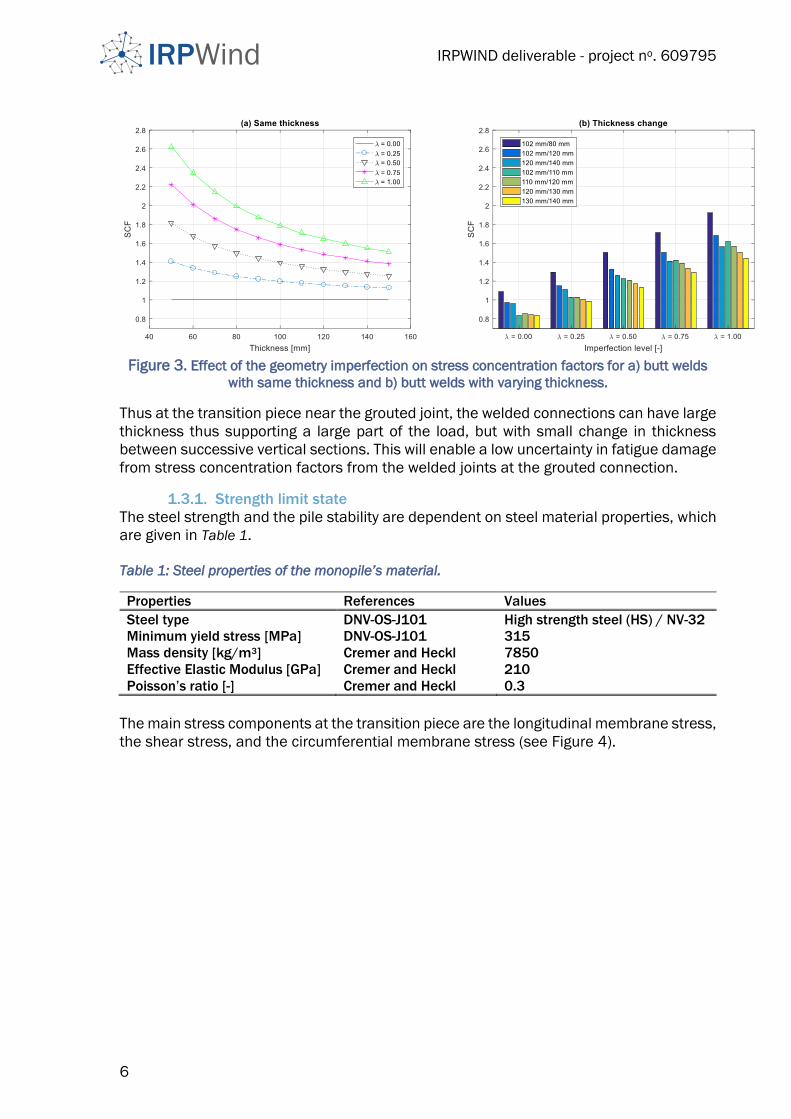
1.4 Metocean conditions Throughout this study, site specific metocean conditions, taken from (De Wries & et.al,
2011) are considered. The operational mean wind speed range varying from 4 m/s to 25
m/s is divided into 11 bins of 2 m/s width. An additional mean wind speed of 42.73 m/s
accounts for extreme storms. The distribution of the wind direction is shown on Figure 5.
IRPWIND deliverable - project no. 609795
8
Figure 5. Distribution of the wind direction (De Wries & et.al, 2011)
Each mean wind speed bin is associated with expected sea states, i.e. significant wave
height (Hs) and peak spectral period (Tp), and an expected annual frequency as shown in
Table 2 Table 3 gives the respective characteristic turbulence intensities observed for each
wind speed bin during normal turbulence and extreme turbulence together with the
turbulence associated with the storm wind speed. The wave height is modelled based on
either the JONSWAP spectrum (under extreme turbulence conditions or extreme wind
conditions) or the Pierson-Moskowitz spectrum (under normal turbulence) at the expected
value of the sea state characteristics conditional on the mean wind speed. The Pierson-
Moskowitz type is used for fatigue load case simulations because of its wide-band energy
distribution, while the JONSWAP type is suitable for ultimate load cases due to its peaked
shape which can promote resonance if the peak coincides with the natural frequencies of
the structure.
Table 2: Environmental Conditions for mean wind speed and wave heights
Wind speed
[m/s]
Expected Significant
height, Hs [m]
Peak period,
Tp [s]
Expected annual
frequency [%]
5 1.140 5.820 10.65
7 1.245 5.715 12.40
9 1.395 5.705 12.88
11 1.590 5.810 12.63
13 1.805 5.975 11.48
15 2.050 6.220 9.36
17 2.330 6.540 7.22
19 2.615 6.850 4.78
21 2.925 7.195 3.57
23 3.255 7.600 2.39
IRPWIND deliverable - project no. 609795
9
25 3.600 7.950 1.70
42.73 (Storm) 9.400 13.700
Table 3: Atmospheric turbulence for normal or extreme model.
Wind
speed [m/s] 5 7 9 11 13 15 17 19 21 23 25 42.73
Normal
Turbulence
Intensity
[%]
18.95 16.75 15.60 14.90 14.40 14.05 13.75 13.50 13.35 13.20 13.00 11.00
Extreme
Turbulence
Intensity
[%]
43.85 33.30 27.43 23.70 21.12 19.23 17.78 16.63 15.71 14.94 14.30 11.00
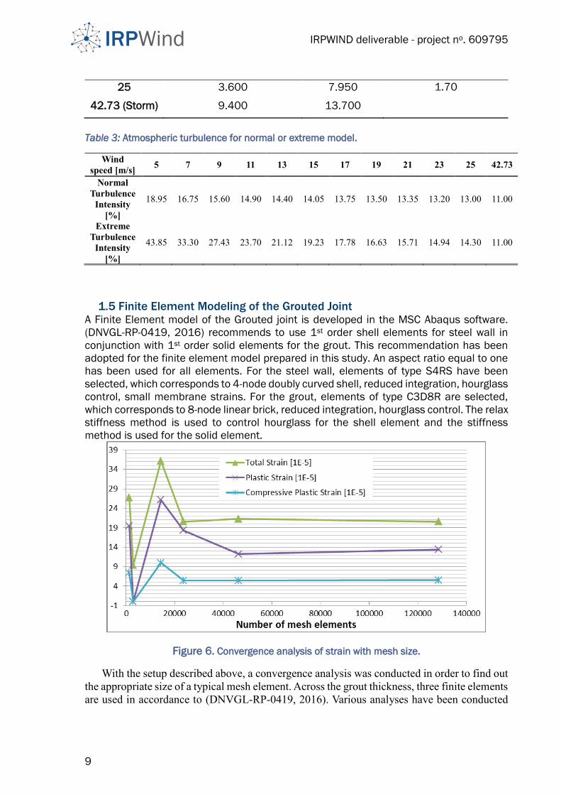
1.5 Finite Element Modeling of the Grouted Joint A Finite Element model of the Grouted joint is developed in the MSC Abaqus software.
(DNVGL-RP-0419, 2016) recommends to use 1st order shell elements for steel wall in
conjunction with 1st order solid elements for the grout. This recommendation has been
adopted for the finite element model prepared in this study. An aspect ratio equal to one
has been used for all elements. For the steel wall, elements of type S4RS have been
selected, which corresponds to 4-node doubly curved shell, reduced integration, hourglass
control, small membrane strains. For the grout, elements of type C3D8R are selected,
which corresponds to 8-node linear brick, reduced integration, hourglass control. The relax
stiffness method is used to control hourglass for the shell element and the stiffness
method is used for the solid element.
Figure 6. Convergence analysis of strain with mesh size.
With the setup described above, a convergence analysis was conducted in order to find out
the appropriate size of a typical mesh element. Across the grout thickness, three finite elements
are used in accordance to (DNVGL-RP-0419, 2016). Various analyses have been conducted
IRPWIND deliverable - project no. 609795
10
with different meshing arrangements. Several structural responses have been monitored at
some selected hotspots; the results at one of them are shown in Figure 7. It can be seen that
above 46500 mesh elements for the grout part, the structural responses converge; this
corresponds to a mesh size of 20 cm x 20 cm for the connection (both grout and steel wall).
1.6 Limit states for the conical grouted joint design
1.6.1 Limit states related to extreme events
In the case of extreme loading, three failure modes can be distinguished for the grouted
connection: failure of the steel-grout contacts, failure of the grout due to compressive stresses,
and excessive vertical displacement of the transition piece relative to the pile. The shear stress,
𝜏, due to the friction between the steel wall and the grout surfaces should be lower than the
shear strength, 𝜏𝑚𝑎𝑥 , of the interface to prevent excessive relative motion between the
transition piece and the pile (Eq. (6a)). This limit state is evaluated for both sides of the grout.
The Tresca stress, 𝜎𝑇𝑟𝑒𝑠𝑐𝑎 , generated in the grout material should be kept lower than the
concrete strength, 𝑓𝑐 , as specified by Eq. (6b). Moreover, the relative settlement, ∆, of the
transition piece with respect to the pile under extreme loading should be moderate and is
limited to a vertical settlement ℎ (See Eq. (7)).
𝑔1 = 𝜏𝑚𝑎𝑥 − 𝜏 (6)
𝑔2 = 𝑓𝑐 − 𝜎𝑇𝑟𝑒𝑠𝑐𝑎 (7)
𝑔3 = ℎ − ∆ (8)
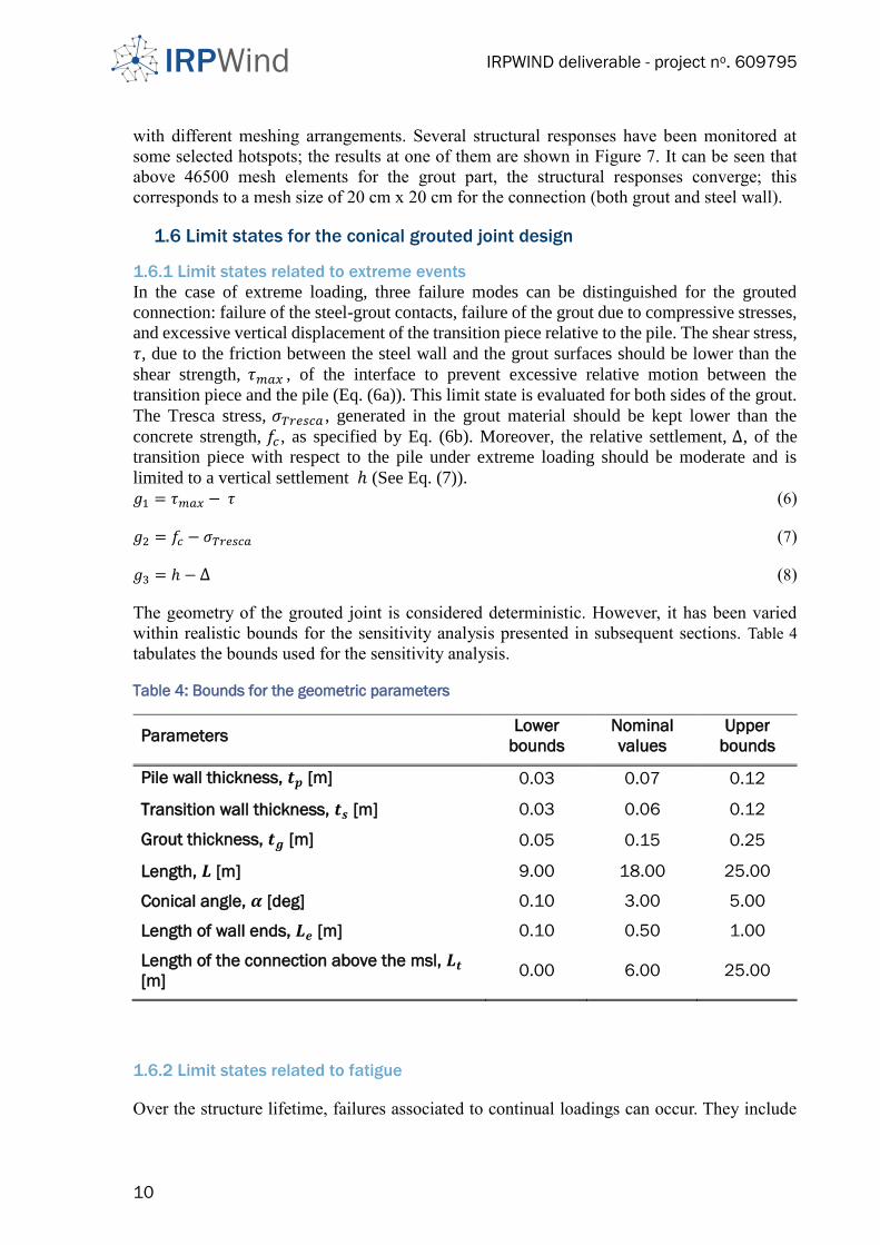
The geometry of the grouted joint is considered deterministic. However, it has been varied
within realistic bounds for the sensitivity analysis presented in subsequent sections. Table 4
tabulates the bounds used for the sensitivity analysis.
Table 4: Bounds for the geometric parameters
Parameters Lower
bounds
Nominal
values
Upper
bounds
Pile wall thickness, 𝒕𝒑 [m] 0.03 0.07 0.12
Transition wall thickness, 𝒕𝒔 [m] 0.03 0.06 0.12
Grout thickness, 𝒕𝒈 [m] 0.05 0.15 0.25
Length, 𝑳 [m] 9.00 18.00 25.00
Conical angle, 𝜶 [deg] 0.10 3.00 5.00
Length of wall ends, 𝑳𝒆 [m] 0.10 0.50 1.00
Length of the connection above the msl, 𝑳𝒕 [m]
0.00 6.00 25.00
1.6.2 Limit states related to fatigue
Over the structure lifetime, failures associated to continual loadings can occur. They include

IRPWIND deliverable - project no. 609795
11
the wear of the grout surfaces in contact with steel walls, the reduction of the grout elastic
modulus due to material degradation, the fatigue of the grout material, and the progressive
vertical displacement of the transition piece relative to the pile as observed in some commercial
wind systems. The friction at the contact faces abrades the grout surfaces. The wear rate is
function of shear stress, which is proportional to the normal pressure exerted from one layer
to another. In this paper, the wear phenomenon is not investigated as a more sophisticated finite
element model is required for an accurate prediction of the phenomenon.
Two types of deterioration are engendered by continual loadings on grout material, fatigue
damage and degradation, which are evaluated independently one to the other. The concrete
degradation corresponds to a variation (diminution) of elastic modulus with the possibility of
material recovery. As the word ‘grade’ is generally used to characterize grout material strength,
the term ‘degradation’ refers to the loss of its elastic modulus. For the fatigue damage, the S-
N curves have been calibrated based on samples that have been subjected to loadings till
fatigue failure. During the experiments, the sample materials have been deteriorated
continually and no full healing has been periodically assumed. So the extrapolation of the
fatigue damage includes the progressive degradation of the grout material. Therefore, fatigue
analyses do not require the monitoring of the damage parameters related to the degradation.
However, it is relevant to monitor the damage parameters to check the crack apparition on the
grout.
The reduction of the grout stiffness will be monitored based on the evolution of the material
degradation parameters. It is important to keep the severely affected areas marginal in the grout
in order to preserve the bending stiffness of the substructure. A change of the substructure
bending stiffness can be noticed by following the lateral displacement of the interface for
example. Subjected to cyclic loadings, the connection engenders cyclic stresses that induce
fatigue in the materials. The accumulated fatigue, D25, in the grout during the intended lifetime,
calculated according to the Palmgren-Miner assumption should be lower than one (See Eq. 8)).
The rate of progression of the long term vertical settlement, δ, of the transition along the pile
should be close to zero so that over years, the initial gap, g, between the pile top edge and the
brackets (See Eq. (9)) does not completely close.
𝑔4 = 1.00 − 𝐷25 (9)
𝑔5 = 𝑔 − 𝛿ℎ (10)
1.7 Design for Fatigue of the Grouted Joint The occurrences of plastic strain generate degradation either of compressive (𝑑𝑐) or of tensile
(𝑑𝑡) types in the grout material. The equivalent degradation (𝑑), which combines the effect of
the compressive and of the tensile degradation, alters the elastic stiffness of the concrete:
𝐃𝑒𝑙|𝑡+∆𝑡 = (1 − 𝑑|𝑡+∆𝑡)𝐃𝑒𝑙|𝑡, where 𝐃𝑒𝑙 is the material stiffness matrix.
The scalar degradation variable, 𝑑 , is computed based on the tensile and compressive
degradation variables: (1 − 𝑑) = (1 − 𝑠𝑡𝑑𝑐)(1 − 𝑠𝑐𝑑𝑡). 𝑑𝑐 and 𝑑𝑡 are taken as the maxima
between their respective previous state values and the present state values obtained by
interpolation 𝑠𝑡 = 1 − 𝑤𝑡𝑟() and 𝑠𝑐 = 1 − 𝑤𝑐(1 − 𝑟()) . 𝑤𝑡 and 𝑤𝑐 are the recovery
factor. 𝑟() = ∑ ⟨𝑖⟩3𝑖=1 /∑ |𝑖|
3𝑖=1 is a stress weight factor, equal to one if all principal stress
components 𝑖, (𝑖 = 1, 2, 3) are positive, or zero if they are negative. ⟨∙⟩ is the Macaulay
bracket.

IRPWIND deliverable - project no. 609795
12
Time [s] 0 - 300 375 600 Legend
Compressive
damage
Tensile
damage
Degradation
variable
Figure 7. Degradation of the concrete material in the grout over time.
Fatigue damage accumulates over lifetime due to cyclic stresses presented above. (DNVGL-
ST-0126, 2016) proposes an algorithm to estimate the total damage. The characteristic
number of cycles to failure is calculated from:
log𝑁 = Y, Y < X
Y(1 + 0.2(𝑌 − 𝑋)), Y ≥ X (11)
𝑌 = 𝐶1 (1 −𝜎𝑚𝑎𝑥
0.8𝑓𝑐𝑛/𝛾𝑚) / (1 −
𝜎𝑚𝑖𝑛
0.8𝑓𝑐𝑛/𝛾𝑚); 𝑋 = 𝐶1/ (1 −
𝜎𝑚𝑖𝑛0.8𝑓𝑐𝑛𝛾𝑚
+ 0.1𝐶1); 𝑓𝑐𝑛 = 𝑓𝑐𝑘 (1 −𝑓𝑐𝑘
600)
where
𝜎𝑚𝑎𝑥, 𝜎𝑚𝑖𝑛 = are respectively the largest value of the maximum principal compressive stress
during a stress cycle within the stress block and the smallest compressive
stress in the same direction during this stress cycle. They are to be individually
set to zero if they belong to the tensile range;
𝛾𝑚= 1.5 is the safety factor associated to the grout material;
𝑓𝑐𝑘 is the characteristic grout cylinder strength measured in MPa;
𝐶1 = calibration factor. For structures in water, 𝐶1 = 10.0 for compression-
compression range and 𝐶1 = 8.0 for compression-tension range.
The damage accumulated over one year is linearly aggregated using Eq. (8); and the
lifetime is calculated as 𝐿𝑓 = 𝐷1−1 and 𝐷25 = 25𝐷1.
𝐷1 = 𝛾𝐹𝐹 ∑𝑛𝑖(∆𝜎) 𝑡𝑖(∆𝜎)
𝑁𝑖(∆𝜎) 𝑖 (12)
where 𝛾𝐹𝐹 = 3.0 is the fatigue reserve factor and 𝑡𝑖(∆𝜎) is the occurrence frequency in one
year of stress range ∆𝜎, which is counted 𝑛𝑖(∆𝜎) times in the simulation time.
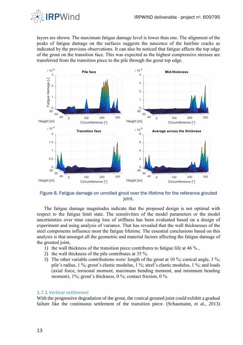
Figure 8 presents the spatial distribution of the fatigue damage accumulated over 25 years
on an unrolled grout accounting for the full directionality of the loads. As the grout has been
meshed in three layers across its thickness, the respective fatigue damage levels of the different
IRPWIND deliverable - project no. 609795
13
layers are shown. The maximum fatigue damage level is lower than one. The alignment of the
peaks of fatigue damage on the surfaces suggests the nascence of the hairline cracks as
indicated by the previous observations. It can also be noticed that fatigue affects the top edge
of the grout on the transition face. This was expected as the highest compressive stresses are
transferred from the transition piece to the pile through the grout top edge.
Figure 8. Fatigue damage on unrolled grout over the lifetime for the reference grouted
joint.
The fatigue damage magnitudes indicate that the proposed design is not optimal with
respect to the fatigue limit state. The sensitivities of the model parameters or the model
uncertainties over time causing loss of stiffness has been evaluated based on a design of
experiment and using analysis of variance. That has revealed that the wall thicknesses of the
steel components influence most the fatigue lifetime. The essential conclusions based on this
analysis is that amongst all the geometric and material factors affecting the fatigue damage of
the grouted joint,
1) the wall thickness of the transition piece contributes to fatigue life at 46 % ,
2) the wall thickness of the pile contributes at 35 %.
3) The other variable contributions were: length of the grout at 10 %; conical angle, 3 %;
pile’s radius, 1 %; grout’s elastic modulus, 1 %; steel’s elastic modulus, 1 %; and loads
(axial force, torsional moment, maximum bending moment, and minimum bending
moment), 1%; grout’s thickness, 0 %; contact friction, 0 %.
1.7.1 Vertical settlement
With the progressive degradation of the grout, the conical grouted joint could exhibit a gradual
failure like the continuous settlement of the transition piece. (Schaumann, et al., 2013)
IRPWIND deliverable - project no. 609795
14
observed a continuous settlement of the transition piece on a cylindrical connection without
shear keys where the passive shear resistance was due to coulomb friction and chemical
adhesion. They have explained that the vertical displacement is caused by the reduction of
coulomb friction when the transition piece approaches its neutral position, where the
operational loads are small.
For the case of the conical grouted connection under the assumption that the shear
resistance is only due to coulomb friction, a large amount of shear resistance is permanently
due to the structural weight. Therefore, it is expected that with a sufficient conical angle, the
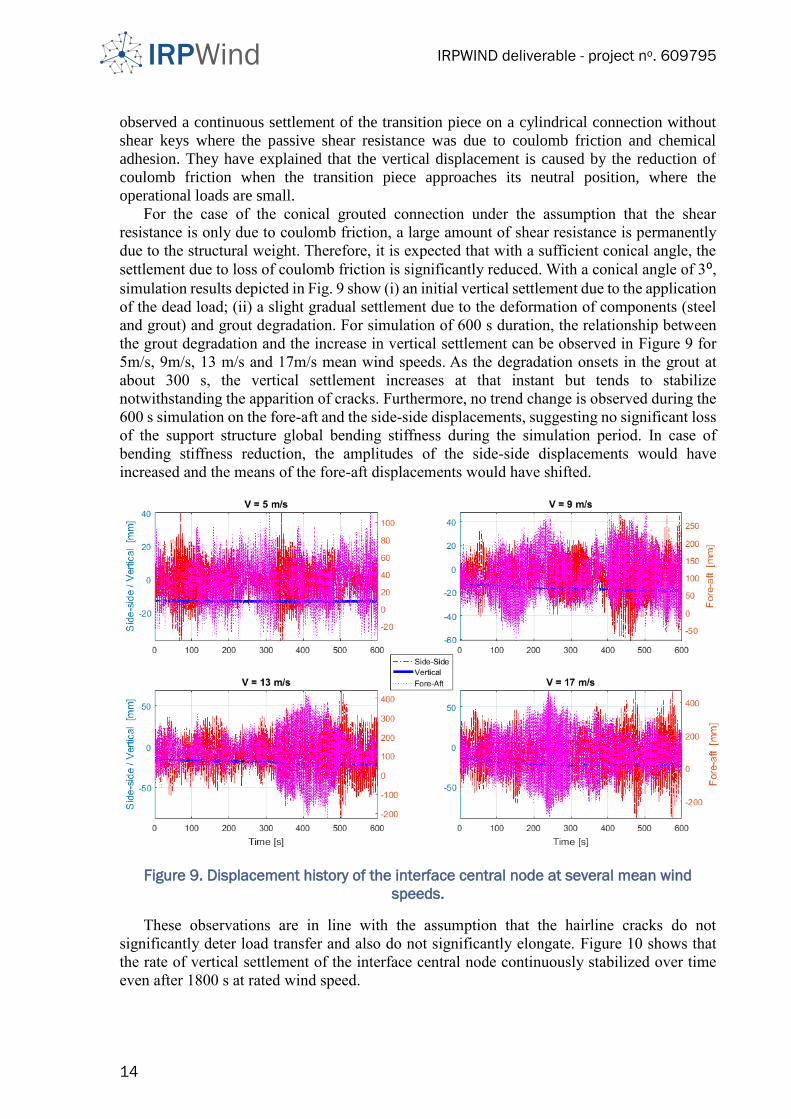
settlement due to loss of coulomb friction is significantly reduced. With a conical angle of 3⁰, simulation results depicted in Fig. 9 show (i) an initial vertical settlement due to the application
of the dead load; (ii) a slight gradual settlement due to the deformation of components (steel
and grout) and grout degradation. For simulation of 600 s duration, the relationship between
the grout degradation and the increase in vertical settlement can be observed in Figure 9 for
5m/s, 9m/s, 13 m/s and 17m/s mean wind speeds. As the degradation onsets in the grout at
about 300 s, the vertical settlement increases at that instant but tends to stabilize
notwithstanding the apparition of cracks. Furthermore, no trend change is observed during the
600 s simulation on the fore-aft and the side-side displacements, suggesting no significant loss
of the support structure global bending stiffness during the simulation period. In case of
bending stiffness reduction, the amplitudes of the side-side displacements would have
increased and the means of the fore-aft displacements would have shifted.
Figure 9. Displacement history of the interface central node at several mean wind
speeds.
These observations are in line with the assumption that the hairline cracks do not
significantly deter load transfer and also do not significantly elongate. Figure 10 shows that
the rate of vertical settlement of the interface central node continuously stabilized over time
even after 1800 s at rated wind speed.

IRPWIND deliverable - project no. 609795
15
Figure 10. Displacement history of the interface central node at 11 m/s mean wind
speed during 1800 s.
As the grout conical angle is varied from 1⁰ to 4⁰, the loading corresponding to 11 m/s mean
wind speed is applied on the structure during 600 s of simulations and the displacement of the
interface is monitored. Depicted in Figure 11, the results show that both the initial settlement
and the settlement rate reduce as the conical angle increases. For small conical angles, the
settlement fails to stabilize during the 600 s, suggesting a continuous vertical displacement till
failure. This indicates the necessity to choose a conical angle of at least 3 degs. to guarantee
grouted joint stability.
Figure 11. Influence of the conical angle on the vertical displacement of the interface for
the reference grouted joint.
1.8 Design for Extremes
1.8.1. Dimensionality reduction and parametrization
Load assessment carried out in HAWC2 under metocean conditions described by Table 2
results in load time series collected at the monopile locations described in Fig.12. The locations
are numbered from 1 to 11 from bottom to top (interface). For each location, six load time
IRPWIND deliverable - project no. 609795
16
series are obtained corresponding to each degree of freedom. Ideally, the ultimate structural
responses should be obtained as the “maximum” of the structural response time series
generated in the structure subjected to a set of load time series. This requires that the finite
element analysis is done for 600 s for a given set of load time series, which is extremely
computationally expensive.
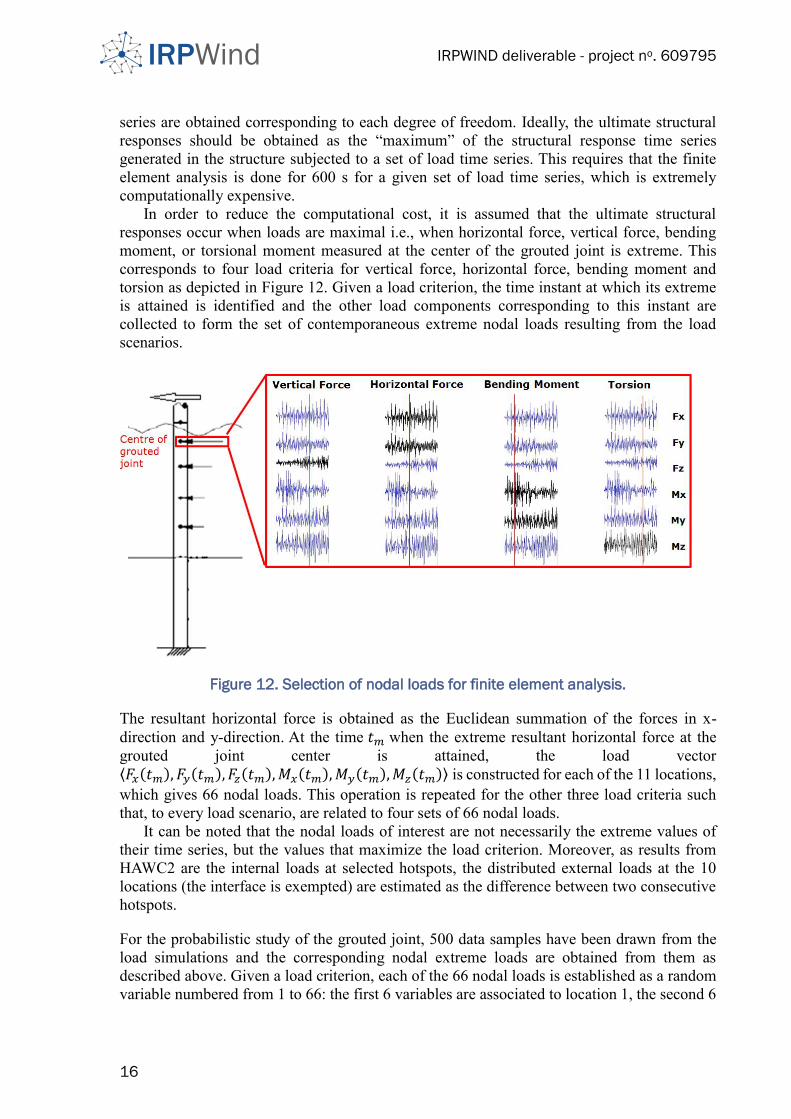
In order to reduce the computational cost, it is assumed that the ultimate structural
responses occur when loads are maximal i.e., when horizontal force, vertical force, bending
moment, or torsional moment measured at the center of the grouted joint is extreme. This
corresponds to four load criteria for vertical force, horizontal force, bending moment and
torsion as depicted in Figure 12. Given a load criterion, the time instant at which its extreme
is attained is identified and the other load components corresponding to this instant are
collected to form the set of contemporaneous extreme nodal loads resulting from the load
scenarios.
Figure 12. Selection of nodal loads for finite element analysis.
The resultant horizontal force is obtained as the Euclidean summation of the forces in x-
direction and y-direction. At the time 𝑡𝑚 when the extreme resultant horizontal force at the
grouted joint center is attained, the load vector ⟨𝐹𝑥(𝑡𝑚), 𝐹𝑦(𝑡𝑚), 𝐹𝑧(𝑡𝑚),𝑀𝑥(𝑡𝑚),𝑀𝑦(𝑡𝑚),𝑀𝑧(𝑡𝑚)⟩ is constructed for each of the 11 locations,
which gives 66 nodal loads. This operation is repeated for the other three load criteria such
that, to every load scenario, are related to four sets of 66 nodal loads.
It can be noted that the nodal loads of interest are not necessarily the extreme values of
their time series, but the values that maximize the load criterion. Moreover, as results from
HAWC2 are the internal loads at selected hotspots, the distributed external loads at the 10
locations (the interface is exempted) are estimated as the difference between two consecutive
hotspots.
For the probabilistic study of the grouted joint, 500 data samples have been drawn from the
load simulations and the corresponding nodal extreme loads are obtained from them as
described above. Given a load criterion, each of the 66 nodal loads is established as a random
variable numbered from 1 to 66: the first 6 variables are associated to location 1, the second 6
IRPWIND deliverable - project no. 609795
17
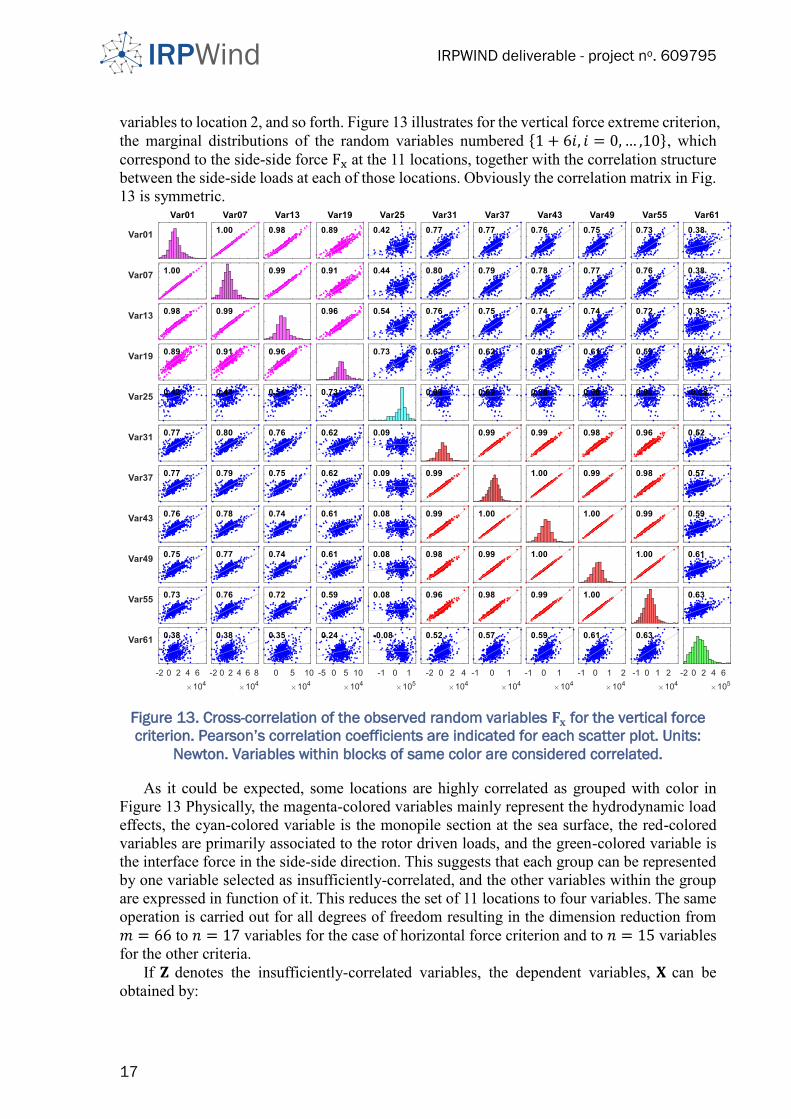
variables to location 2, and so forth. Figure 13 illustrates for the vertical force extreme criterion,
the marginal distributions of the random variables numbered 1 + 6𝑖, 𝑖 = 0,… ,10 , which
correspond to the side-side force Fx at the 11 locations, together with the correlation structure
between the side-side loads at each of those locations. Obviously the correlation matrix in Fig.
13 is symmetric.
Figure 13. Cross-correlation of the observed random variables 𝐅𝐱 for the vertical force
criterion. Pearson’s correlation coefficients are indicated for each scatter plot. Units:
Newton. Variables within blocks of same color are considered correlated.
As it could be expected, some locations are highly correlated as grouped with color in
Figure 13 Physically, the magenta-colored variables mainly represent the hydrodynamic load
effects, the cyan-colored variable is the monopile section at the sea surface, the red-colored
variables are primarily associated to the rotor driven loads, and the green-colored variable is
the interface force in the side-side direction. This suggests that each group can be represented
by one variable selected as insufficiently-correlated, and the other variables within the group
are expressed in function of it. This reduces the set of 11 locations to four variables. The same
operation is carried out for all degrees of freedom resulting in the dimension reduction from
𝑚 = 66 to 𝑛 = 17 variables for the case of horizontal force criterion and to 𝑛 = 15 variables
for the other criteria.
If 𝐙 denotes the insufficiently-correlated variables, the dependent variables, 𝐗 can be
obtained by:
IRPWIND deliverable - project no. 609795
18
𝐗𝑚×1 = 𝜶𝑚×𝑛𝐙𝑛×1 + 𝛃𝑚×1 (13)
where 𝜶 is the matrix of the scale factors obtained as the ratio of 𝐗’s standard deviation over
𝐙’s standard deviation; and 𝜷 is the vector of the shifts obtained as the difference between
the 𝐗’s average and the 𝛂𝐙’s average.
The marginals of the insufficiently-correlated variables are modeled with parametric
probability density functions (PDFs). The Gumbel distribution is suitable to model extreme
values. The difference of two Gumbel distributed variables follows a Logistic distribution. As
nodal loads are obtained as the difference of loads possibly Gumbel-distributed, the Logistic
distribution is applicable. The dependence structure within the sets of insufficiently-correlated
variables, 𝐙 , is captured using Gaussian cupola, which results in the joint probability
distribution of the set of the insufficiently-correlated random variables. Given the correlation
matrix 𝐑 of 𝐙, the Gaussian copula is defined as 𝑐(𝑢1, ⋯ , 𝑢𝑛) = 𝛟𝐑(𝛟−1(𝑢1),⋯ ,𝛟−1(𝑢𝑛)),
where 𝑢𝑖 = 𝐹𝑖(𝑍𝑖); 𝐹𝑖 cumulative distribution function (CDF) of the insufficiently-correlated
variable 𝑍𝑖; 𝛟𝐑(∙) is the joint cumulative distribution function of a n-dimension multivariate
normal distribution with mean vector zero and covariance matrix equal to 𝐑; and 𝛟−1(∙) is the
inverse cumulative distribution function of a standard normal.
1.8.2 Simulation of Extreme Response of Grouted Joint
The accuracy of the constructed dependence structure in Eq. (12) has been evaluated by
comparing the correlation matrix from the observed data versus that of synthetic data simulated
from the constructed joint probability distribution. The root-mean-square deviations (RMSD)
between the correlation matrices of the two data sets are determined to be 1.12 %, 0.85 %,
0.83 %, 0.60 % for the horizontal force, the vertical force, the bending moment, and the
torsional moment criteria, respectively. Thus, random simulations of possible extreme load
combinations at the grouted joint can be run using Eq. (12) for all the load criteria.
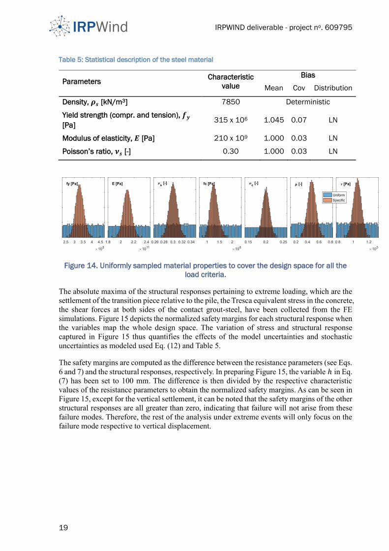
In addition, the variables related to the material properties have been independently and
uniformly sampled between the bounds as per Table 5 and as relevant per the load case. The
results are shown in Figure 14. The geometry-related variables are also independently and
uniformly sampled between the bounds as indicated in The geometry of the grouted joint is
considered deterministic. However, it has been varied within realistic bounds for the sensitivity
analysis presented in subsequent sections. Table 4 tabulates the bounds used for the sensitivity
analysis. With the 500 uniformly sampled variables describing loads, material properties as
given in Figure 14, and geometry parameters described in Table 4, a batch of finite element
simulations have been run in the Abaqus software.
IRPWIND deliverable - project no. 609795
19
Table 5: Statistical description of the steel material
Parameters Characteristic
value
Bias
Mean Cov Distribution
Density, 𝝆𝒔 [kN/m3] 7850 Deterministic
Yield strength (compr. and tension), 𝒇𝒚
[Pa] 315 x 106 1.045 0.07 LN
Modulus of elasticity, 𝑬 [Pa] 210 x 109 1.000 0.03 LN
Poisson’s ratio, 𝝂𝒔 [-] 0.30 1.000 0.03 LN
Figure 14. Uniformly sampled material properties to cover the design space for all the
load criteria.
The absolute maxima of the structural responses pertaining to extreme loading, which are the
settlement of the transition piece relative to the pile, the Tresca equivalent stress in the concrete,
the shear forces at both sides of the contact grout-steel, have been collected from the FE
simulations. Figure 15 depicts the normalized safety margins for each structural response when
the variables map the whole design space. The variation of stress and structural response
captured in Figure 15 thus quantifies the effects of the model uncertainties and stochastic
uncertainties as modeled used Eq. (12) and Table 5.
The safety margins are computed as the difference between the resistance parameters (see Eqs.
6 and 7) and the structural responses, respectively. In preparing Figure 15, the variable ℎ in Eq.
(7) has been set to 100 mm. The difference is then divided by the respective characteristic
values of the resistance parameters to obtain the normalized safety margins. As can be seen in
Figure 15, except for the vertical settlement, it can be noted that the safety margins of the other
structural responses are all greater than zero, indicating that failure will not arise from these
failure modes. Therefore, the rest of the analysis under extreme events will only focus on the
failure mode respective to vertical displacement.

IRPWIND deliverable - project no. 609795
20
Figure 15. Normalized safety margins of the structural responses over the design space.
1.8.3 Prediction of the extreme settlement
From each point of the simulation batch of size N described in the last section, the maximum
vertical displacements ∆𝑖, 𝑖 = 1,… ,𝑁 are collected. Each can be seen as the peak of the time
series of vertical displacement related to a given mean wind speed. In this sense, they are
reasonably assumed to be independent and identically distributed random variables. With this
assumption, the extreme value theory applies and the random variable ∆𝑖 follows the
cumulative distribution function (CDF):
𝐹s(𝑥|𝜇, 𝜎, 휀) = exp[−𝑧(𝑥|𝜇, 𝜎, 휀)] (14)
𝜇, 𝜎, 휀 are the parameters of the CDF 𝐹s, and 𝑧 is a function of the random variable 𝑥. For the
traditional extreme value families (Gumbel, Frechet, and Weibull (Natarajan & Holley, 2008),
𝑧(𝑥|𝜇, 𝜎, 휀) = (1 + 휀𝑥−𝜇
𝜎)−1 𝜀⁄
with 𝑥 ∈
[𝜇 −𝜎
𝜀 +∞), 휀 > 0
(−∞ +∞), 휀 → 0
(−∞ 𝜇 −𝜎
𝜀], 휀 < 0
(15)
As a substitute of Eq. (11), studies (Natarajan & Holley, 2008), have proposed a quadratic
shape for 𝑧 such that
𝑧(𝑥|𝜇, 𝜎, 휀) = 𝜇 𝑥2 + 𝜎 𝑥 + 휀 with 𝑥 ∈ (−∞ +∞) (16)
and have shown its appropriateness and its robustness for fitting extreme structural responses
of various wind turbine structures. Furthermore, the empirical CDF is generally constructed
by sorting the random variables ∆𝑖 in ascending order so that each is associated to a rank 𝑑𝑖. The following expression of the empirical CDF can be written:
𝐹e(∆) =𝑑
𝑁+1 (17)
Equating Eq. (10) and Eq. (13), the parameters 𝜇, 𝜎, 휀 can be obtained by regression. Hence
the probability of exceeding a given vertical displacement is calculated as 𝐺(∆) = 1 − 𝐹s(∆). As per modern standards, the targeted annual reliability index is about 𝛽0 = 3.3 , which
corresponds to a targeted failure probability 𝑃𝑓0 = 4.93 × 10⁻⁴. This means that in order to
be safe, the grouted joint should be able to undergo a vertical displacement up to ∆0=𝐺−1(𝑃𝑓0) without any consequence on its structural integrity. With an allowable settlement

IRPWIND deliverable - project no. 609795
21
ℎ ≤ ∆0 (see Eq. (4)) failure is not prevented; the design should provide an allowable settlement
greater than or equal to ∆0.
The reliability index is determined for a given design, with given material and geometry
properties. In order to evaluate the survival distribution function (SDF), 𝐺, the grouted joint
design with similar properties have been binned with respect to grout length, which is the
primary influencing parameter. Four bins of equal width are constructed over the length range
[9 m, 25 m] and the corresponding SDFs are fitted as illustrated in Figure 16. For each bin, the
settlement threshold required to achieve the targeted annual reliability index is obtained by
graphical projection.
Figure 16. Sensitivity coefficients of the structural responses with respect to the
geometry and material variables. The fitted curves are in red and the data point are in
blue.
For each bin range, Table 6 gives the settlement thresholds. Thus for the reference grouted
joint, which has 18 m grout length, provisions for 72 mm of vertical displacement should be
made. Further, the gap between the pile top edge and the jacking brackets should be at least
72 mm to ensure that it possesses sufficient reliability. The settlement of the transition piece
will then not create any consequence on the overall joint structural integrity. Within this
framework of this study, allowing a settlement of 72 mm is possible as the other failure modes
associated to extreme events are proven improbable. In general, if a high settlement cannot be
afforded, a longer grout length should be used to achieve the required reliability.
Table 6: Settlement thresholds for each grout length bin
Bin No Bin 1 Bin 2 Bin 3 Bin 4
Bin range [9 m, 13 m) [13 m, 17 m) [17 m, 21 m) [21 m, 25 m]
Settlement threshold 115 mm 110 mm 72 mm 32 mm
The major conclusions from this study are summarized in (Wandji, et al., 2018).

IRPWIND deliverable - project no. 609795
22
2. Reliability assessment of grouted joint with shear keys
The cylindrical grouted connection with shear keys for 10MW reference wind turbine was
developed and detailed in (Santos, et al., 2017). The deterministic design and stochastic
reliability analysis in the following sections are performed based on the initial design
detailed in (Santos, et al., 2017), with environmental input given in Table 2 and Table 3.
The present report mostly focuses on further development of the stochastic concrete
fatigue reliability model using (CEB-fip, 2013) as basis for the model formulation.
Furthermore, an updated steel fatigue reliability model, based on fracture mechanics, is
described and improvements over the simplified model from (Santos, et al., 2017) are
discussed.
The cylindrical grouted joint with shear keys is initially evaluated deterministically for
concrete grout fatigue resistance. The evaluation is done using two methodologies, based
namely on (DNVGL-ST-C502, 2017) and (CEB-fip, 2013). Such evaluation is necessary for
comparison purposes between the two methodologies and in order to identify the most
critical locations in the concrete for further reliability assessment.
2.1 Target reliability levels
This section describes the required target reliability levels for design of structural wind
turbine components, see also D7.4.1. The basis for the description is the requirements in
the CDW/FDIS version of the IEC 61400-1 ed. 4 (IEC61400-1, 2017) wind turbine
standard which are also described in the background document (Sørensen, 2014).The
target reliability level can generally be given in terms of a maximum annual probability of
failures (i.e. reference time equal to 1 year) or a maximum lifetime probability of failure
(i.e. for wind turbines a reference time equal to 20 – 25 years). For civil and structural
engineering standards / codes of practice where failure can imply risk of loss of human
lives target reliabilities are generally given based on annual probabilities. Examples of
reliability levels required (implicitly) in some relevant standards / codes (for normal
consequence / reliability class) are:
• For fixed steel offshore structures, see e.g. ISO 19902 (ISO 19902, 2007) an indicated
annual probability of failure for manned structures is PF ~ 3 10-5 or β = 4.0. For
structures that are unmanned or evacuated in severe storms and where other
consequences of failure are not very significant the indicated annual probability of
failure PF ~ 5 10-4 or β = 3.3.
• (DNV-OS-J101, 2014) states: ‘The target safety level for structural design of support
structures and foundations for wind turbines to the normal safety class according to
this standard is a nominal annual probability of failure of 10-4. This target safety is the
level aimed at for structures, whose failures are ductile, and which have some reserve
capacity. The target safety level of 10-4 is compatible with the safety level implied by
DNV-OS-C101 for unmanned structures’. It is noted that (DNVGL-ST-0126, 2016) does
not contain a target reliability level, but opens for the use of reliability-based design.
• (JCSS, 2002) and (ISO 2394, 2015) recommend reliability requirements based on
annual failure probabilities for structural systems for ultimate limit states These are
based on optimization procedures and on the assumption that for almost all

IRPWIND deliverable - project no. 609795
23
engineering facilities the only reasonable reconstruction policy is systematic rebuilding
or repair.
It should be noted that the -values (and the corresponding failure probabilities) are
formal / notional numbers, intended primarily as a tool for developing consistent design
rules, rather than giving a description of the structural failure frequency. E.g. the effect of
human errors is not included. Human errors in design and execution are assumed to be
detected by quality control.
For wind turbines the risk of loss of human lives in case of failure of a structural element
is generally very small. Further, it can be assumed that wind turbines are systematically
reconstructed in case of collapse or end of lifetime. In that case also target reliabilities
based on annual probabilities should be used, see JCSS, (JCSS, 2002). The optimal
reliability level can be found by considering representative cost-benefit based optimization
problems where the life-cycle expected cost of energy is minimized. Also, the following
assumptions are made in (IEC61400-1, 2017) and (Sørensen, 2014):
• A systematic reconstruction policy is used (a new wind turbine is erected in case of
failure or expiry of lifetime).
• Consequences of a failure are only economic (no fatalities and no pollution).
• Cost of energy is important which implies that the relative cost of safety measures can
be considered large (material cost savings are important).
• Wind turbines are designed to a certain wind turbine class, i.e. not all wind turbines
are ‘designed to the limit’.
Based on these considerations the target reliability level corresponding to a minimum
annual probability of failure is recommended to be Pf=5 10-4 corresponding to an annual
reliability index equal to 3.3. This reliability level corresponds to minor / moderate
consequences of failure and moderate / high cost of safety measure.
2.1 Deterministic assessment of concrete grout fatigue resistance
2.1.1 Deterministic assessment according to DNVGL-ST-C502
(DNVGL-ST-C502, 2017) recommends the following procedure to estimate the fatigue
damage within the concrete grouted connection:
max
510 1 1
min
5
1
log
1
rd
rd
C fN C
C f
(18)
10 10 1 2 10 1log log logN N C for N X (19)
1
min1
5
1 0.1rd
CX
CC f
(20)
2 10 11 0.2 log 1.0C N X (21)
,
cnrd
c fat
ff
(22)

IRPWIND deliverable - project no. 609795
24
1600
ckcn ck
ff f
(23)
1
ki i
i i
t nD
N
(24)
here N is the design life in terms of number of cycles; σmax, σmin are the numerically largest
and smallest compressive stresses; frd is the design compressive fatigue strength of
concrete; C5 is fatigue strength parameter, for grout = 0.8 in the absence of fatigue tests;
C1 factor is taken = 12 for concrete structures in air, = 10 for structures in water with
stress variation in compression-compression range and = 8 for stress variation in
compression-tension range; fck is the characteristic compressive concrete strength; fcn is
normalized compressive strength of concrete; γc,fat is the partial safety factor for concrete
in fatigue = 1.5; ti is the service life; ni is the expected annual number of particular stress
cycles; η is cumulative damage ratio, = 0.33 for structures with no access for inspection.
It should be noted that following the methodology from (DNVGL-ST-C502, 2017), all tensile
stress ranges are individually set to 0 and the effect of grout fatigue due to tension is only
accounted for through the use of a lowered C1 factor in eq.(18). The following Figure 17
shows the resulting accumulated damage throughout the analyzed section of the
cylindrical grouted connection.
Figure 17: Accumulated damage (left) and a zoom of most critical location (right).
It is clear that the most critical cross-section of the grout is located just below the first
level of shear keys with significantly lower fatigue damage in subsequent lower levels of
shear keys. Using grout with 100MPa characteristic compressive strength the design of
the connection seems sub-optimal, accumulated damage over 25-year lifetime is orders
of magnitude lower than η=0.33, thus implying that further optimization of the design
would be necessary – possibly through reduction of grout strength or changes in shear
key geometry/placement. However, it is important to further evaluate the most critically
loaded location in terms of expected reliability - this is done in the following sections.
2.1.2 Deterministic assessment according to fib Model Code 2010
(DNVGL-ST-0126, 2016) allows the use of Model Code 2010 (CEB-fip, 2013) for
concrete/grout fatigue evaluation with certain modifications to the concrete fatigue
strength - eq.(25-26). Furthermore, a design fatigue factor DFF=1 should be used, instead
of 3, giving allowable cumulative damage ratio η=1.0 in contrast with η=0.33 used by
(DNVGL-ST-C502, 2017).
IRPWIND deliverable - project no. 609795
25
, ( ) 1400
ckck fat sus red cc ck
ff t f
(25)
,
,
,
ck fat
cd fat
C fat
ff
(26)
, ,2.12 ln 1 0.1 /td fat red cc cm C fatf f (27)
Here βred – strength reduction due to specific interaction between concrete grout and steel
= 0.8; βsus – strength reduction coefficient due to sustained load (mismatch between
testing and real load frequencies) = 0.85; βcc – coefficient for considering time dependent
load (=1.0 after 28 days for this case); γc is the partial safety factor for concrete grout in
fatigue =1.5.
According to (CEB-fip, 2013) the following procedure for fatigue evaluation of concrete
grout should be followed:
log1
n1
10 Ri
ni
Ni
tD
(28)
,max
8log 1 log 8
1R cdN S for N compression only
Y
(29)
,max ,min
,min
,min
8 ln 10log 8 log log 8
1
cd cd
R cs
cd
S SN Y S for N compression only
Y Y S
(30)
,max ,max ,maxlog 9 1 0.026R cd ct cN S for compression tension
(31)
,max ,max ,maxlog 12 1 0.026R td ct cN S for compression pure tension
(32)
,min
2
,min ,min
0.45 1.8
1 1.8 0.3
cd
cd cd
SY
S S
(33)
,min ,max ,max
, ,max ,max
, , ,
Ed LOAD c Ed LOAD c Ed LOAD ct
c min c ct
cd fat cd fat td fat
C C CS S S
f f f
(34)
Here t – service time in years; ni – number of stress range/mean stress combinations in
a given year (from Markov Matrix); Scd,min, Scd,max – normalized design minimum and
maximum compressive stress levels, respectively; σc,min, σc,max – minimum and maximum
compressive stresses in MPa; σct,max – maximum tensile stress in MPa; γEd - partial safety
factor for fatigue loading =1.1, according to (CEB-fip, 2013).
A significant difference between (CEB-fip, 2013) and (DNVGL-ST-C502, 2017)
methodologies for concrete fatigue assessment is that (CEB-fip, 2013), instead of setting
tensile stresses to 0 (together with proposing a more conservative SN curve), proposes
SN curves (eq.(31-32)) for concrete in compression-tension and compression-pure
tension fatigue loading. For comparison purposes between (CEB-fip, 2013) and (DNVGL-
ST-C502, 2017), initially only compression-compression loading is considered and only
eq.(29-30) are used. The following Figure 18 shows the resulting accumulated damage of
the grouted connection.

IRPWIND deliverable - project no. 609795
26
Figure 18: Accumulated damage (left) and a zoom of most critical location (right), Compression -
Compression SN curve (CEB-fip, 2013).
While the location of the most critically loaded concrete nodes remains the same (upper-
most level of shear keys with decreasing accumulated damage for lower shear key levels),
(CEB-fip, 2013) gives lower accumulated damage results. The design still seems sub-
optimal using concrete with 100MPa compressive strength - accumulated damage is
orders of magnitude lower than η=1.0. It should also be noted that due to magnitude of
stresses in the concrete, the joint operates in log N > 8 region thus eq.(30) contributes
most to the damage accumulation. Further, compression-tension and compression-pure
tension fatigue loading is included in the accumulated damage calculation. Figure 19
below shows the resulting accumulated damage of compression-tension stress
components.
Figure 19: Accumulated damage (left) and a zoom of most critical location (right). Compression -
Tension SN curve (CEB-fip, 2013).
Most critical nodes when compression-tension stress components are included in the
analysis appears to be roughly in the middle of the grouted joint (z = -10.43m), in between
shear keys on the opposing sides of the concrete grout. It is also clear that the
accumulated damage due to tensile fatigue stresses is significantly higher, while still being
acceptably below η=1.0, than in the case where only compressive stresses were
considered. This implies that a thorough tensile fatigue analysis is necessary when
designing cylindrical grouted connections with shear keys. Figure 20 shows the
accumulated damage of compression-pure tension stress components.

IRPWIND deliverable - project no. 609795
27
Figure 20: Accumulated damage (left) and a zoom of most critical location (right). Compression –
Pure Tension SN curve (CEB-fip, 2013).
It is seen from the figure above that there are significant tensile regions around shear
keys where compression-pure tensions stress states produce notable, while lower than
compression-tension stress states, contributions to accumulated damage. This again
implies that it is important not to disregard tensile fatigue stresses when assessing
grouted connection fatigue resistance/life.
Figure 21: Accumulated damage (left) and a zoom of most critical location (right). Combined
loading.
As the largest contribution to accumulated damage is coming from compression-tension
stress ranges/states, results in Figure 21 are quite similar to Figure 20. The most critical
nodes are selected from results in Figure 21 and used in further sections for concrete
fatigue reliability evaluation.
2.2 Reliability assessment of grouted joint – Concrete grout fatigue
Fatigue reliability is assessed using SN curves proposed in (CEB-fip, 2013), modified to
accommodate stochastic parameters, together with Miner’s rule for damage
accumulation. The limit state equation is defined by the following equations:
0)(),( tDDtXg cr (35)

IRPWIND deliverable - project no. 609795
28
log1
N0
10 Ri
ni
Ni
tg
(36)
1,max 1 1 1log 1 log ( )
1R c
AN S for N A
Y
(37)
,max ,min1
1 ,min 1 1 1
,min
ln 10log log log ( )
1
c c
R c
c
S SAN A Y S for N A
Y Y S
(38)
2 ,max 2 ,max ,maxlog 1 0.026R c ct cN A S for
(39)
3 ,max 3 ,max ,maxlog 1 0.026R ct ct cN A S for
(40)
2
min,min,
min,
3.08.11
8.145.0
cc
c
SS
SY
(41)
,min ,max ,max
, ,max ,max
, ,
LOAD c LOAD c LOAD ct
c min c ct
c fat c fat tm
C C CS S S
f f f
(42)
, 1 / 400c fat red sus cc cm cmf f f
(43)
, 2.12 ln 1 0.1t fat red cc cmf f
(44)
t – service time in years; Ni – number of stress range/mean stress combinations in a given
year (from Markov Matrix); Sc,min, Sc,max – normalized minimum and maximum compressive
stress levels, respectively; σc,min, σc,max – minimum and maximum compressive stresses in
MPa; fc,fat – compressive concrete fatigue strength in MPa; fcm – mean compressive
concrete strength in MPa; βred – strength reduction due to specific interaction between
concrete grout and steel;βsus – strength reduction coefficient due to sustained load
(mismatch between testing and real load frequencies); βcc – coefficient for considering
time dependent load (=1.0 after 28 days for this case).
2.2.1 Stochastic model for concrete grout fatigue
Stochastic model parameters for SN curves are estimated from data available in the
literature, namely the compression-compression SN curve parameters (A1 and ε1) are
estimated from (Lantsoght, 2014) and (Slot & Andersen, 2014) as detailed in (Santos, et
al., 2017) and (Rodriguez, et al., 2018), whereas SN curve parameters for compression-
tension and compression-pure tension (A1, A2, ε1 and ε2) are estimated from (Cornelissen,
1984). The statistical parameters (Ak and σεk) are estimated using the Maximum
Likelihood Method for data sets available of (Ni, Sc,max,i). The likelihood function for
compression-tension and compression- pure tension is in general written:
( ),max,
1
( ),max,
1
( , ) 1 log
1 log
F
R
n
k i k c t i k i
i
n
k c t i k i
i
L A P A S N
P A S N
(45)

IRPWIND deliverable - project no. 609795
29
where nF is the number of tests where failure occurs, and nR is the number of tests where
failure did not occur (run-outs). The total number of tests is n= nF+ nR. Ai and σεk are
obtained from the optimization problem
,max ( , )
k k
k kA
L A
(46)
or using the log-likelihood function
,max ln ( , )
k k
k kA
L A
(47)
which can be solved using a standard nonlinear optimizer (e.g. NLPQL algorithm, see
(Schittkowski, 1986). Because the parameters Ak, and σεk are determined using a limited amount
of data; they are subject to statistical uncertainty. Since the parameters are estimated by the
maximum-likelihood method, they become asymptotically (number of data should be > 25 – 30)
normally distributed stochastic variables with expected values equal to the maximum-likelihood
estimators and covariance matrix equal to, see e.g. (Lindley, 1976). 2
1 ,
, , 2
,
k k k k k
k k k k
k k k k
A A A
A A
A A
C H
(48)
,k kAH is the Hessian matrix with second-order derivatives of the log-likelihood function.
σAk and σσεk denote the standard deviations of Ak and σεk, respectively, and ,k kA
is the
correlation coefficient between Ak and σεk. Table 7 shows a summary of the estimated SN
curve parameters together with other parameters necessary to fully define the stochastic
model for concrete fatigue reliability assessment. Furthermore, Figure 22 shows the
stochastic SN curves based on equations from (CEB-fip, 2013) and stochastic parameters
from Table 7.
Table 7: Parameters for probabilistic concrete fatigue damage model.
Variable Distribution Expected value Standard
deviation /
COV
Comment
Compression-Compression
A1 N 8.91 SD=0.16 SN curve parameter
ε1 N 0 SD=1.17 Model error
Compression-Tension
A2 N 8.64 SD=0.37 SN curve parameter
ε2 N 0 SD=0.66 Model error
Compression-Pure Tension
A3 N 19.11 SD=1.28 SN curve parameter
ε3 N 0 SD=0.80 Model error
Common parameters
fcm LN 123 COV= 0.12 Mean concrete comp. str.
Model uncertainties
Δ LN 1 COV = 0.30 Model uncertainty Miner’s
rule
CLOAD LN 1 COV= 0.08 Model uncertainty fatigue
load
IRPWIND deliverable - project no. 609795
30
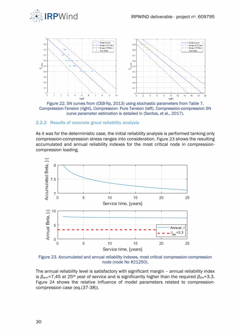
Figure 22. SN curves from (CEB-fip, 2013) using stochastic parameters from Table 7.
Compression-Tension (right), Compression- Pure Tension (left). Compression-compression SN
curve parameter estimation is detailed in (Santos, et al., 2017).
2.2.2 Results of concrete grout reliability analysis
As it was for the deterministic case, the initial reliability analysis is performed tanking only
compression-compression stress ranges into consideration. Figure 23 shows the resulting
accumulated and annual reliability indexes for the most critical node in compression-
compression loading.
Figure 23. Accumulated and annual reliability indexes, most critical compression-compression
node (node No #21250).
The annual reliability level is satisfactory with significant margin – annual reliability index
is βann=7,45 at 25th year of service and is significantly higher than the required βlim=3.3.
Figure 24 shows the relative influence of model parameters related to compression-
compression case (eq.(37-38)).
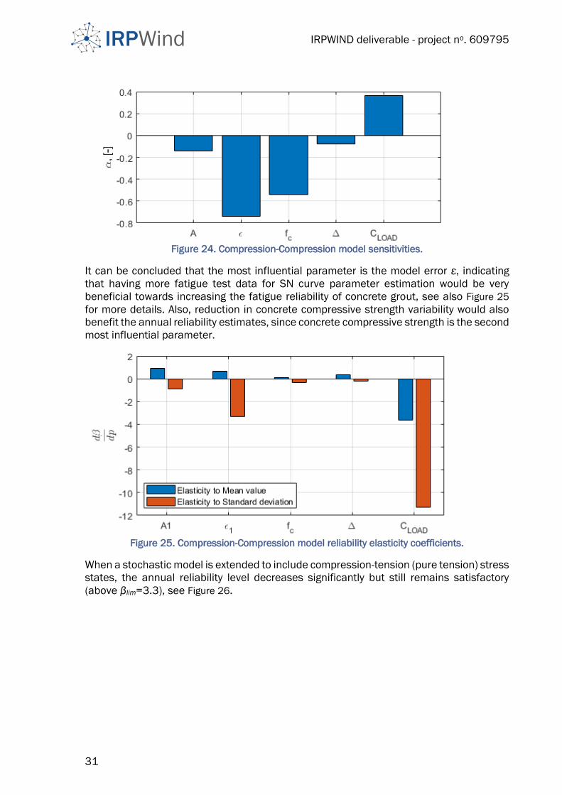
IRPWIND deliverable - project no. 609795
31
Figure 24. Compression-Compression model sensitivities.
It can be concluded that the most influential parameter is the model error ε, indicating
that having more fatigue test data for SN curve parameter estimation would be very
beneficial towards increasing the fatigue reliability of concrete grout, see also Figure 25
for more details. Also, reduction in concrete compressive strength variability would also
benefit the annual reliability estimates, since concrete compressive strength is the second
most influential parameter.
Figure 25. Compression-Compression model reliability elasticity coefficients.
When a stochastic model is extended to include compression-tension (pure tension) stress
states, the annual reliability level decreases significantly but still remains satisfactory
(above βlim=3.3), see Figure 26.
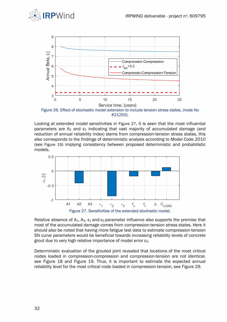
IRPWIND deliverable - project no. 609795
32
Figure 26. Effect of stochastic model extension to include tension stress states, (node No
#21250).
Looking at extended model sensitivities in Figure 27, it is seen that the most influential
parameters are A2 and ε2 indicating that vast majority of accumulated damage (and
reduction of annual reliability index) stems from compression-tension stress states, this
also corresponds to the findings of deterministic analysis according to Model Code 2010
(see Figure 19) implying consistency between proposed deterministic and probabilistic
models.
Figure 27. Sensitivities of the extended stochastic model.
Relative absence of A1, A3, ε1 and ε3 parameter influence also supports the premise that
most of the accumulated damage comes from compression-tension stress states. Here it
should also be noted that having more fatigue test data to estimate compression-tension
SN curve parameters would be beneficial towards increasing reliability levels of concrete
grout due to very high relative importance of model error ε2.
Deterministic evaluation of the grouted joint revealed that locations of the most critical
nodes loaded in compression-compression and compression-tension are not identical,
see Figure 18 and Figure 19. Thus, it is important to estimate the expected annual
reliability level for the most critical node loaded in compression-tension, see Figure 29.
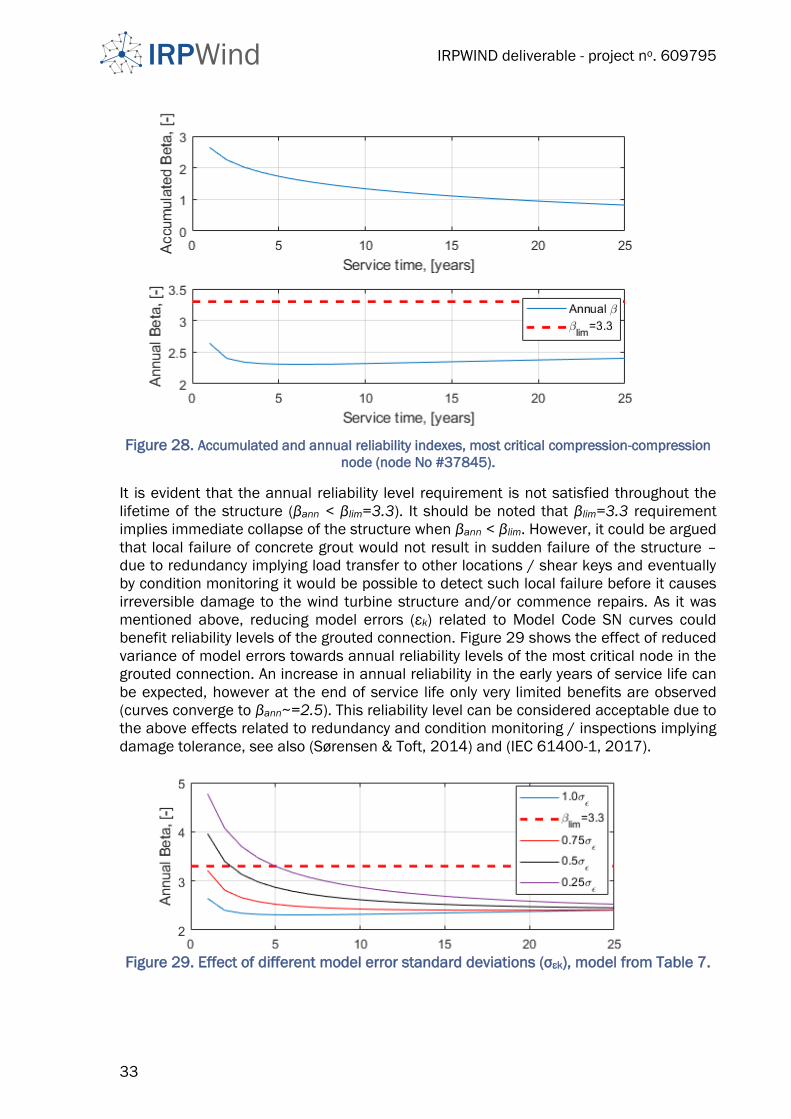
IRPWIND deliverable - project no. 609795
33
Figure 28. Accumulated and annual reliability indexes, most critical compression-compression
node (node No #37845).
It is evident that the annual reliability level requirement is not satisfied throughout the
lifetime of the structure (βann < βlim=3.3). It should be noted that βlim=3.3 requirement
implies immediate collapse of the structure when βann < βlim. However, it could be argued
that local failure of concrete grout would not result in sudden failure of the structure –
due to redundancy implying load transfer to other locations / shear keys and eventually
by condition monitoring it would be possible to detect such local failure before it causes
irreversible damage to the wind turbine structure and/or commence repairs. As it was
mentioned above, reducing model errors (εk) related to Model Code SN curves could
benefit reliability levels of the grouted connection. Figure 29 shows the effect of reduced
variance of model errors towards annual reliability levels of the most critical node in the
grouted connection. An increase in annual reliability in the early years of service life can
be expected, however at the end of service life only very limited benefits are observed
(curves converge to βann~=2.5). This reliability level can be considered acceptable due to
the above effects related to redundancy and condition monitoring / inspections implying
damage tolerance, see also (Sørensen & Toft, 2014) and (IEC 61400-1, 2017).
Figure 29. Effect of different model error standard deviations (σεk), model from Table 7.

IRPWIND deliverable - project no. 609795
34
Additionally, Figure 30 and Figure 31 below show the reliability elasticity coefficients
related to cases shown in in Figure 29.
Figure 30. Reliability elasticity coefficients for 1.0 σε case in Figure 29.
Figure 31. Reliability elasticity coefficients for 0.5 σε case in Figure 29.
It is clear that reliability indexes are quite sensitive to changes in mean values and
standard deviations of model parameters. Obviously increasing the intercept of SN curve
and X axis (mean value of parameter A2) or total allowable accumulated damage (mean
value of parameter Δ) would increase the reliability index, as would also an increase in
mean value of the model error ε2, as is evident from positive mean value elasticity
coefficients. Conversely, increase of standard deviation of any of these stochastic
variables would result in significant reduction of grouted joint reliability indexes.
2.3 Reliability assessment of grouted joint – fatigue of welded steel details
A deterministic analysis of the steel part of the grouted connection is performed and
detailed in (Santos, et al., 2017). (Santos, et al., 2017) also contains the initial reliability
assessment of the steel components of the grouted connection – a simplified fracture
mechanics based streel fatigue model is calibrated to give the same (or as close as
possible) annual reliability levels throughout the lifetime. In the following section a more
advanced fracture mechanics model is used to investigate whether such more complex
model would be beneficial. This section uses SN curve based probabilistic model results
as basis to calibrate the updated fracture mechanics based fatigue crack growth model.
2.3.1 Stochastic model for steel fatigue
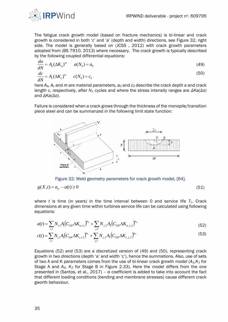
IRPWIND deliverable - project no. 609795
35
The fatigue crack growth model (based on fracture mechanics) is bi-linear and crack
growth is considered in both ‘c’ and ‘a’ (depth and width) directions, see Figure 32, right
side. The model is generally based on (JCSS , 2012) with crack growth parameters
adopted from (BS 7910, 2013) where necessary. The crack growth is typically described
by the following coupled differential equations:
00)()( aNaKAdN
da m
aa (49)
00)()( cNcKAdN
dc m
cc (50)
here Aa, Ac and m are material parameters, a0 and c0 describe the crack depth a and crack
length c, respectively, after N1 cycles and where the stress intensity ranges are ΔKa(Δσ)
and ΔKa(Δσ).
Failure is considered when a crack grows through the thickness of the monopile/transition
piece steel and can be summarized in the following limit state function:
Figure 32: Weld geometry parameters for crack growth model, [64].
0)(),( taatXg cr (51)
where t is time (in years) in the time interval between 0 and service life TL. Crack
dimensions at any given time within turbines service life can be calculated using following
equations:
21
1,
2,,22,
1,
1,,11,)(m
j
jaSIFj
m
i
iaSIFi KCANKCANta (52)
21
1,
2,,22,
1,
1,,11,)(m
j
jcSIFj
m
i
icSIFi KCANKCANtc (53)
Equations (52) and (53) are a discretized version of (49) and (50), representing crack
growth in two directions (depth ‘a’ and width ‘c’), hence the summations. Also, use of sets
of two A and K parameters comes from the use of bi-linear crack growth model (A1,K1 for
Stage A and A2, K2 for Stage B in Figure 2.33). Here the model differs from the one
presented in (Santos, et al., 2017) – α coefficient is added to take into account the fact
that different loading conditions (bending and membrane stresses) cause different crack
gworth behaviour.
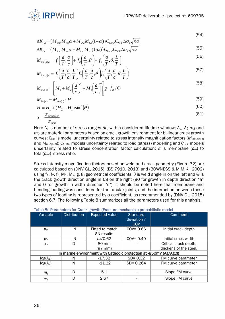
IRPWIND deliverable - project no. 609795
36
, (1 )i a kma ma kba ba Load SCF i iK M M M M C C a
(54)
, (1- )i c kmc mc kbc bc Load SCF i iK M M M M C C a (55)
T
L
T
af
T
af
c
a
T
afM abkm ,,,, 221)(
(56)
T
L
c
a
T
af
c
a
T
af
T
L
a
c
T
afM cbkm ,,,,,,, 221)(
(57)
/
4
3
2
21)( fgc
aM
c
aMMM cma
(58)
HMM cmacba )()( (59)
qHHHH sin)( 121 (60)
membrane
total
(61)
Here Ni is number of stress ranges Δσi within considered lifetime window; A1, A2 m1 and
m2 are material parameters based on crack growth environment for bi-linear crack growth
curves; CSIF is model uncertainty related to stress intensity magnification factors (Mkm(b)a(c)
and Mm(b)a(c)); CLOAD models uncertainty related to load (stress) modelling and CSCF models
uncertainty related to stress concentration factor calculation; α is membrane (σm) to
total(σtot) stress ratio.
Stress intensity magnification factors based on weld and crack geometry (Figure 32) are
calculated based on (DNV GL, 2015), (BS 7910, 2013) and (BOWNESS & M.M.K., 2002)
using f1, f2, f3, M1, M2, g, fΘ geometrical coefficients. θ is weld angle in on the left and Θ is
the crack growth direction angle in 68 on the right (90 for growth in depth direction “a”
and 0 for growth in width direction “c”). It should be noted here that membrane and
bending loading was considered for the tubular joints, and the interaction between these
two types of loading is represented by α coefficient, as recommended by (DNV GL, 2015)
section 6.7. The following Table 8 summarizes all the parameters used for this analysis.
Table 8: Parameters for Crack growth (Fracture mechanics) probabilistic model
Variable Distribution Expected value Standard
deviation /
COV
Comment
a0 LN Fitted to match
SN results
COV= 0.66 Initial crack depth
c0 LN a0/0.62 COV= 0.40 Initial crack width
acr D 80 mm
(97 mm)
- Critical crack depth,
thickens of the steel.
In marine environment with Cathodic protection at -850mV (Ag/AgCl)
log(A1) N -17.32 SD= 0.32 FM curve parameter
log(A2) N -11.22 SD= 0.264 FM curve parameter
D 5.1 - Slope FM curve
D 2.67 - Slope FM curve
1m
2m
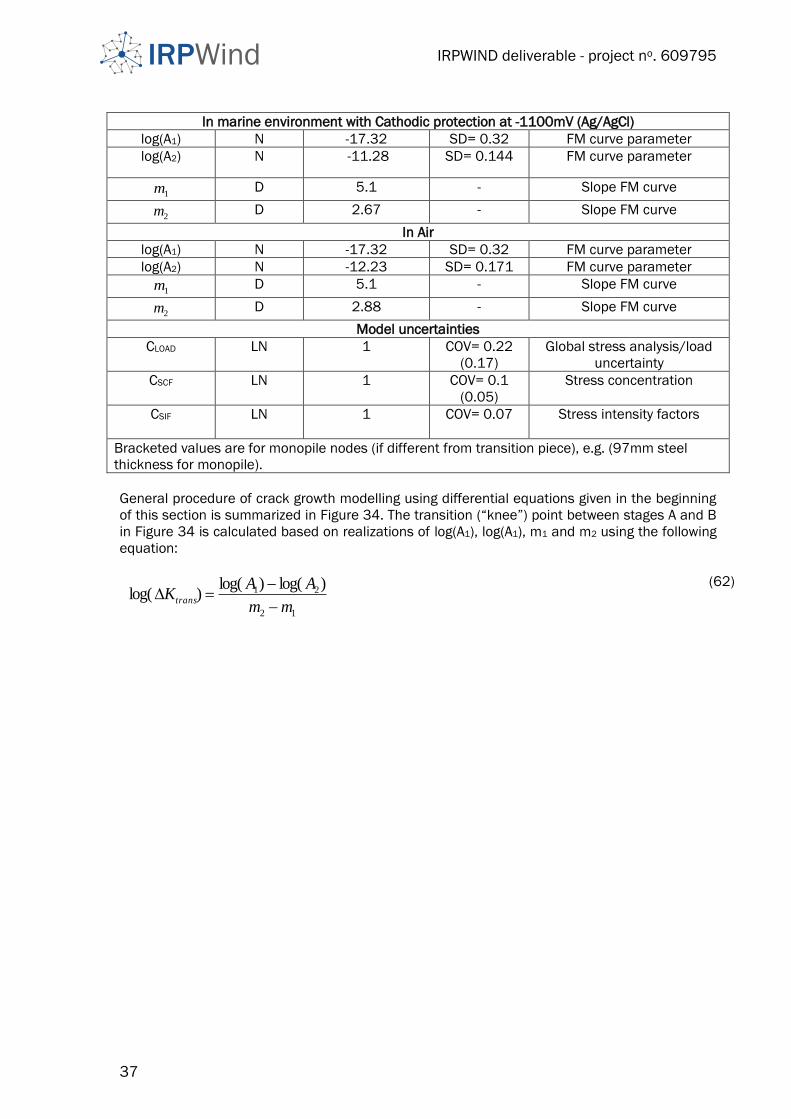
IRPWIND deliverable - project no. 609795
37
In marine environment with Cathodic protection at -1100mV (Ag/AgCl)
log(A1) N -17.32 SD= 0.32 FM curve parameter
log(A2) N -11.28 SD= 0.144 FM curve parameter
D 5.1 - Slope FM curve
D 2.67 - Slope FM curve
In Air
log(A1) N -17.32 SD= 0.32 FM curve parameter
log(A2) N -12.23 SD= 0.171 FM curve parameter
D 5.1 - Slope FM curve
D 2.88 - Slope FM curve
Model uncertainties
CLOAD LN 1
COV= 0.22
(0.17)
Global stress analysis/load
uncertainty
CSCF LN 1
COV= 0.1
(0.05)
Stress concentration
CSIF LN 1
COV= 0.07 Stress intensity factors
Bracketed values are for monopile nodes (if different from transition piece), e.g. (97mm steel
thickness for monopile).
General procedure of crack growth modelling using differential equations given in the beginning
of this section is summarized in Figure 34. The transition (“knee”) point between stages A and B
in Figure 34 is calculated based on realizations of log(A1), log(A1), m1 and m2 using the following
equation:
12
21 )log()log()log(
mm
AAKtrans
(62)
1m
2m
1m
2m
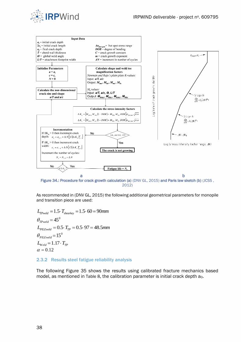
IRPWIND deliverable - project no. 609795
38
a b Figure 34.: Procedure for crack growth calculation (a) (DNV GL, 2015) and Paris law sketch (b) (JCSS ,
2012)
As recommended in (DNV GL, 2015) the following additional geometrical parameters for monopile
and transition piece are used:
1.5 1.5 60 90TPweld shearkeyL T mm
045TPweld
0.5 0.5 97 48.5PILEweld TPL T mm
015PILEweld
TPWeld TL 17.1
0.12
2.3.2 Results steel fatigue reliability analysis
The following Figure 35 shows the results using calibrated fracture mechanics based
model, as mentioned in Table 8, the calibration parameter is initial crack depth a0.
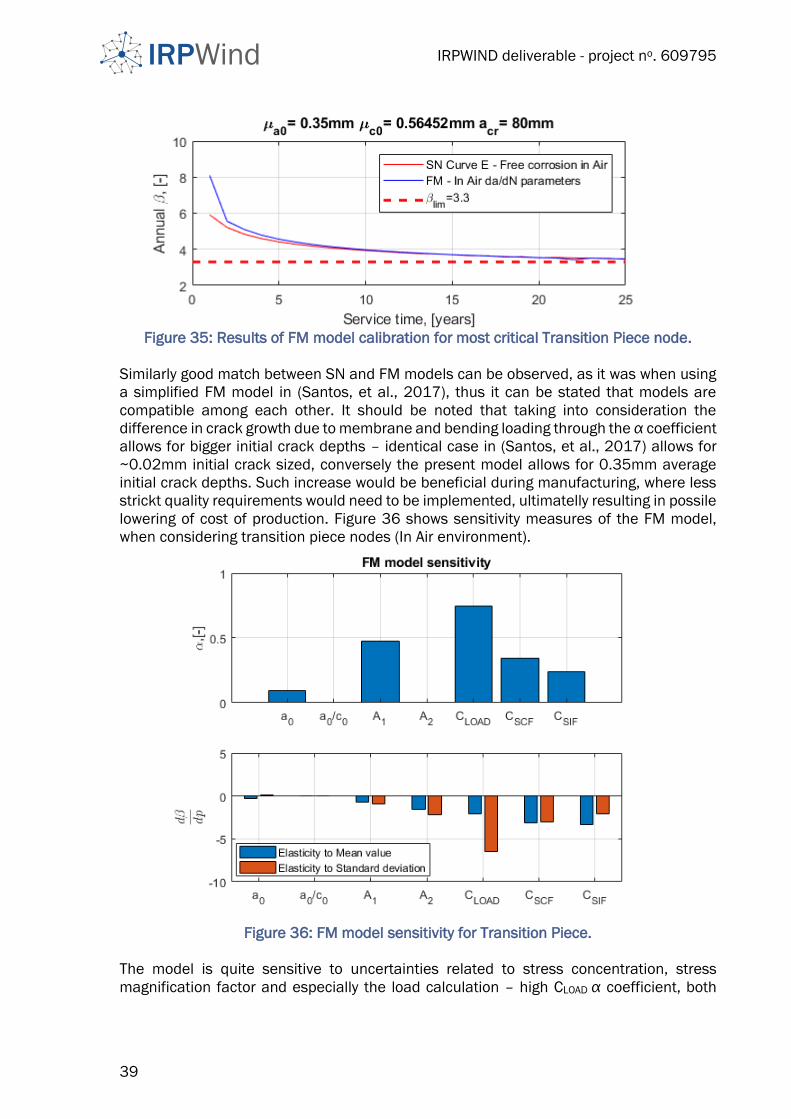
IRPWIND deliverable - project no. 609795
39
Figure 35: Results of FM model calibration for most critical Transition Piece node.
Similarly good match between SN and FM models can be observed, as it was when using
a simplified FM model in (Santos, et al., 2017), thus it can be stated that models are
compatible among each other. It should be noted that taking into consideration the
difference in crack growth due to membrane and bending loading through the α coefficient
allows for bigger initial crack depths – identical case in (Santos, et al., 2017) allows for
~0.02mm initial crack sized, conversely the present model allows for 0.35mm average
initial crack depths. Such increase would be beneficial during manufacturing, where less
strickt quality requirements would need to be implemented, ultimatelly resulting in possile
lowering of cost of production. Figure 36 shows sensitivity measures of the FM model,
when considering transition piece nodes (In Air environment).
Figure 36: FM model sensitivity for Transition Piece.
The model is quite sensitive to uncertainties related to stress concentration, stress
magnification factor and especially the load calculation – high CLOAD α coefficient, both
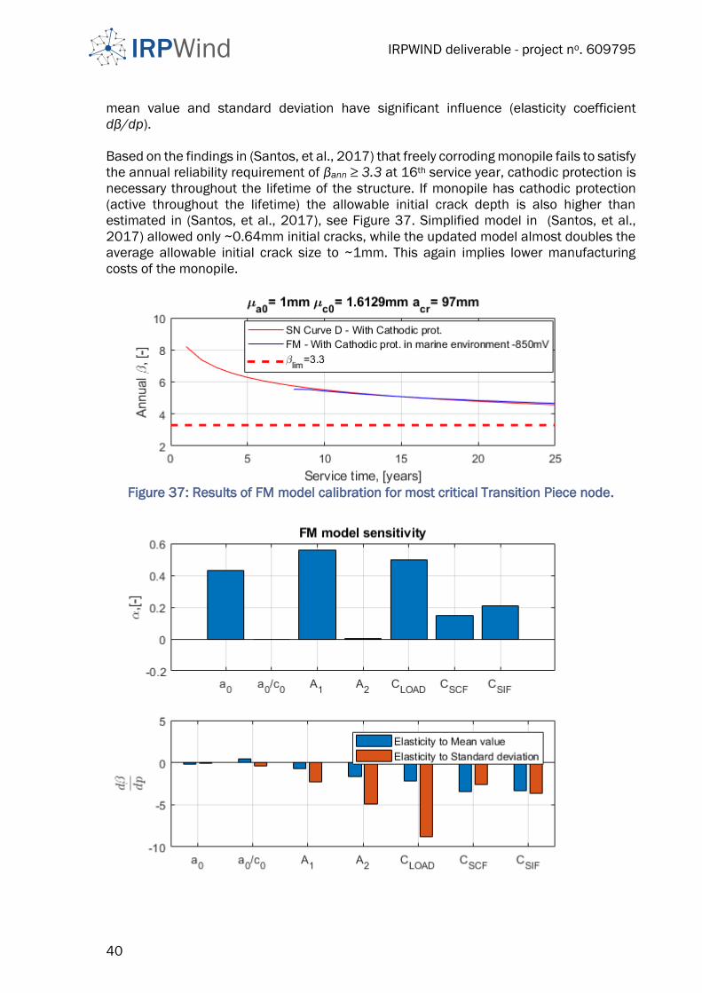
IRPWIND deliverable - project no. 609795
40
mean value and standard deviation have significant influence (elasticity coefficient
dβ/dp).
Based on the findings in (Santos, et al., 2017) that freely corroding monopile fails to satisfy
the annual reliability requirement of βann ≥ 3.3 at 16th service year, cathodic protection is
necessary throughout the lifetime of the structure. If monopile has cathodic protection
(active throughout the lifetime) the allowable initial crack depth is also higher than
estimated in (Santos, et al., 2017), see Figure 37. Simplified model in (Santos, et al.,
2017) allowed only ~0.64mm initial cracks, while the updated model almost doubles the
average allowable initial crack size to ~1mm. This again implies lower manufacturing
costs of the monopile.
Figure 37: Results of FM model calibration for most critical Transition Piece node.
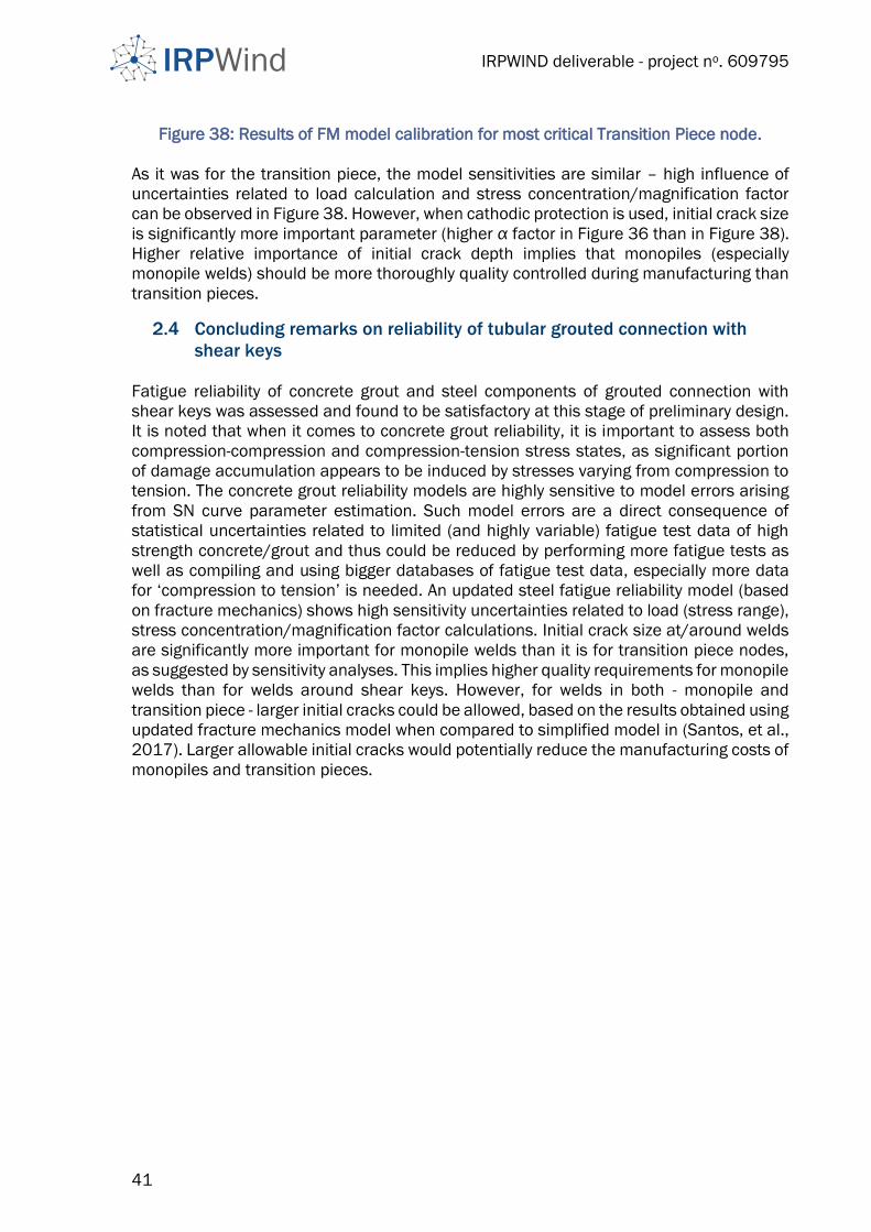
IRPWIND deliverable - project no. 609795
41
Figure 38: Results of FM model calibration for most critical Transition Piece node.
As it was for the transition piece, the model sensitivities are similar – high influence of
uncertainties related to load calculation and stress concentration/magnification factor
can be observed in Figure 38. However, when cathodic protection is used, initial crack size
is significantly more important parameter (higher α factor in Figure 36 than in Figure 38).
Higher relative importance of initial crack depth implies that monopiles (especially
monopile welds) should be more thoroughly quality controlled during manufacturing than
transition pieces.
2.4 Concluding remarks on reliability of tubular grouted connection with
shear keys
Fatigue reliability of concrete grout and steel components of grouted connection with
shear keys was assessed and found to be satisfactory at this stage of preliminary design.
It is noted that when it comes to concrete grout reliability, it is important to assess both
compression-compression and compression-tension stress states, as significant portion
of damage accumulation appears to be induced by stresses varying from compression to
tension. The concrete grout reliability models are highly sensitive to model errors arising
from SN curve parameter estimation. Such model errors are a direct consequence of
statistical uncertainties related to limited (and highly variable) fatigue test data of high
strength concrete/grout and thus could be reduced by performing more fatigue tests as
well as compiling and using bigger databases of fatigue test data, especially more data
for ‘compression to tension’ is needed. An updated steel fatigue reliability model (based
on fracture mechanics) shows high sensitivity uncertainties related to load (stress range),
stress concentration/magnification factor calculations. Initial crack size at/around welds
are significantly more important for monopile welds than it is for transition piece nodes,
as suggested by sensitivity analyses. This implies higher quality requirements for monopile
welds than for welds around shear keys. However, for welds in both - monopile and
transition piece - larger initial cracks could be allowed, based on the results obtained using
updated fracture mechanics model when compared to simplified model in (Santos, et al.,
2017). Larger allowable initial cracks would potentially reduce the manufacturing costs of
monopiles and transition pieces.
IRPWIND deliverable - project no. 609795
42
3. Reliability of piles and substructures under consideration of soil
parameters
Within Work Package WP7.4 and the corresponding Deliverables D74.2 reliability based
assessment of the foundation piles and the support structure should be conducted. These
analyses are closely linked to Work Package WP7.2 and the corresponding Deliverables
D72.2, since the executed analysis strongly based on the measured data from the
performed foundation pile tests in Work Package WP7.2.
Section 3.1 deals with two major topics, which are focused on the reliability assessment
of the foundation pile with respect to geotechnical ULS design requirements, where
Section 3.2 focusses on the reliability of the substructure while taking the turbine and soil
parameters into account.
3.1 Reliability of the substructure under consideration of the turbine and soil
parameters Within Section 3.1 first, a new model error for the design methods of the axial tension
bearing capacity is derived on basis of the additional incorporated pile load tests
performed in WP7.2. Second, a reliability based study for typical offshore foundation piles
in the North Sea is conducted, where the new derived model error is included. Using the
calculated reliability based results, a new calibration approach regarding a more robust
deterministic design was conducted. Thereby quality factors for the considered
deterministic design methods were derived. These quality factors indicate on basis of the
performed reliability based calculations the reliability regarding the axial tension bearing
capacity within a deterministic design.
Altogether the executed tasks in Section 3.1 can be summarized as follows:
• Determination of a new model error for the tension capacity of offshore piles
• Description of the applied design methods
• Determination of the theoretical tension capacity for the performed pile
load tests in WP7.2
• Derivation of a model error from the calculated and measured data
• Assessment of design methods with respect to deterministic ULS design
• Determination of the reliability index for typical pile dimensions and soil
conditions in the North Sea
• Comparison between the deterministic and reliability based design results
• Derivation of quality factors for the deterministic design methods

IRPWIND deliverable - project no. 609795
43
3.1.1 Introduction
In the near future, several offshore wind farms are planned to be built in the North Sea to
satisfy the demand for a high amount of renewable energy in Germany. As most shallow
depth sea areas have already been exploited, a number of projects will be located in sea
areas with relatively high water depths (exceeding 40 m). For such water depths, jacket
and tripod support structures with mainly axially loaded foundation piles will probably be
employed in most cases.
The axial bearing resistance of such piles is normally estimated according to the
recommendation of API (American Petroleum Institute, 2014) by applying the so termed
“Main Text” method. However, several investigations (e.g. (Lehane, et al., 2005) or
(Cathie, 2012)) have shown that the application of the Main Text method, at least for
foundation piles of wind energy converters, is not reliable and may lead to a significant
deviation compared to the real in situ bearing capacity.
To enhance the reliability of design methods, 4 additional CPT-based design methods,
namely ICP, UWA, Fugro and NGI, were recommended within API (American Petroleum
Institute, 2014). These methods were calibrated on pile field tests, where basically the
skin friction of a pile and the end bearing are estimated on basis of the cone resistance
qc measured in a CPT. It is believed that the proposed CPT-based design methods are
more reliable than the API Main Text method. However, it is emphasized within the API
(American Petroleum Institute, 2014) that care should be taken in the application of these
methods, since experience is limited. Indeed, the application of the CPT-based methods
leads in practice to a high deviation in the required pile length within a design. In this work
package (WP7.4), two major issues are investigated:
First, a new derived model error for the axial tension bearing capacity is obtained from the
model tests performed within WP7.2. These model tests were aligned with the
corresponding boundary conditions for offshore foundation piles in the North Sea as well
as with already available pile load tests in literature. An overview of the performed
complementary pile load tests and already published pile load tests was given in the report
for WP7.2.
Second, a comprehensive study is performed in which different deterministically designed
pile-soil systems are investigated regarding the failure probability with reliability based
approaches. Thereby, a new calibration approach is applied, where quality factors for each
design method are derived. Based on these quality factors, an enhanced evaluation of a
certain design method in question regarding the reliability of the predicted tensile bearing
capacity can be done. Moreover, a more reliable as well as more robust deterministic
design can be achieved by taking the proposed quality factors into. In this work package,
only the tension bearing resistance of offshore foundation piles is investigated.
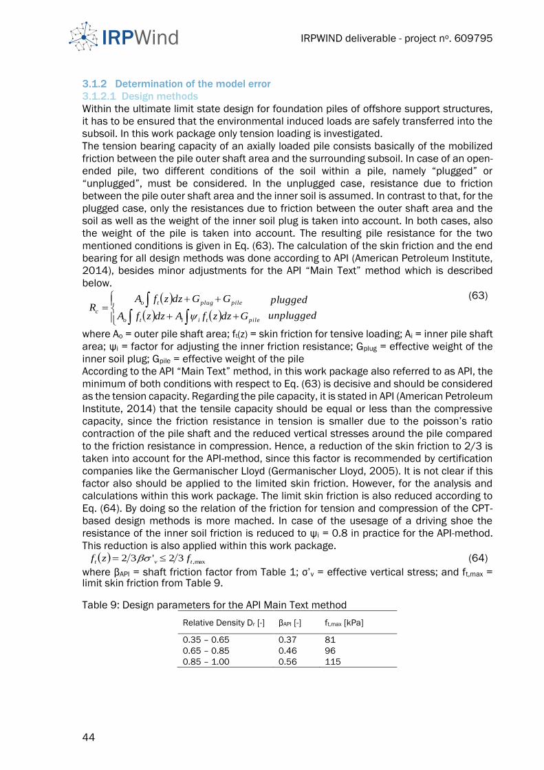
IRPWIND deliverable - project no. 609795
44
3.1.2 Determination of the model error
3.1.2.1 Design methods
Within the ultimate limit state design for foundation piles of offshore support structures,
it has to be ensured that the environmental induced loads are safely transferred into the
subsoil. In this work package only tension loading is investigated.
The tension bearing capacity of an axially loaded pile consists basically of the mobilized
friction between the pile outer shaft area and the surrounding subsoil. In case of an open-
ended pile, two different conditions of the soil within a pile, namely “plugged” or
“unplugged”, must be considered. In the unplugged case, resistance due to friction
between the pile outer shaft area and the inner soil is assumed. In contrast to that, for the
plugged case, only the resistances due to friction between the outer shaft area and the
soil as well as the weight of the inner soil plug is taken into account. In both cases, also
the weight of the pile is taken into account. The resulting pile resistance for the two
mentioned conditions is given in Eq. (63). The calculation of the skin friction and the end
bearing for all design methods was done according to API (American Petroleum Institute,
2014), besides minor adjustments for the API “Main Text” method which is described
below.
unplugged
plugged
GdzzfAdzzfA
GGdzzfAR
piletiito
pileplugto
c
(63)
where Ao = outer pile shaft area; ft(z) = skin friction for tensive loading; Ai = inner pile shaft
area; ψi = factor for adjusting the inner friction resistance; Gplug = effective weight of the
inner soil plug; Gpile = effective weight of the pile
According to the API “Main Text” method, in this work package also referred to as API, the
minimum of both conditions with respect to Eq. (63) is decisive and should be considered
as the tension capacity. Regarding the pile capacity, it is stated in API (American Petroleum
Institute, 2014) that the tensile capacity should be equal or less than the compressive
capacity, since the friction resistance in tension is smaller due to the poisson’s ratio
contraction of the pile shaft and the reduced vertical stresses around the pile compared
to the friction resistance in compression. Hence, a reduction of the skin friction to 2/3 is
taken into account for the API-method, since this factor is recommended by certification
companies like the Germanischer Lloyd (Germanischer Lloyd, 2005). It is not clear if this
factor also should be applied to the limited skin friction. However, for the analysis and
calculations within this work package. The limit skin friction is also reduced according to
Eq. (64). By doing so the relation of the friction for tension and compression of the CPT-
based design methods is more mached. In case of the usesage of a driving shoe the
resistance of the inner soil friction is reduced to ψi = 0.8 in practice for the API-method.
This reduction is also applied within this work package. max,32'32 tvt fzf (64)
where βAPI = shaft friction factor from Table 1; σ’v = effective vertical stress; and ft,max = limit skin friction from Table 9. Table 9: Design parameters for the API Main Text method
Relative Density Dr [-] βAPI [-] ft,max [kPa]
0.35 – 0.65 0.37 81
0.65 – 0.85 0.46 96
0.85 – 1.00 0.56 115

IRPWIND deliverable - project no. 609795
45
The estimation of the relative density from a CPT should be done according to the proposed approach by (Jamiolkowski, et al., 1988) according to Eq. (65):
𝐷𝑟 =1
2.96ln
[
𝑞𝑐 𝑝𝑎⁄
24.94 (𝑝′𝑚𝑝𝑎)0.46
]
(65)
where qc = measured cone tip resistance in kPa; and p‘m = effective mean in-situ soil stress in kPa. In case of the CPT-based design methods, always a plugged condition for the tensile
bearing capacity is assumed. Thereby the weight of the soil plug is indirectly considered
in the outer friction resistance. In contrast to the API Main Text method, the outer skin
friction of the CPT-based design methods was correlated directly with CPT measurements.
The skin friction for the ICP-05, UWA-05 and Fugro-05 method can be calculated according
to Eq. (66). The friction for the NGI-05 method is given by Eq. (67).
dcv
c
o
b
r
a
a
vct
D
zLA
pquzf
tan;max
'
(66)
where σ’v = vertical effective stress in kPa; pa = atmospheric stress 100 kPa; Ar = 1-(Di/Do)² pile displacement ratio; L = embedded pile length in m; z = current depth in m; Do = pile outer diameter; δcv = interface friction angle; a,b,c,d,u,υ = Parameters according to Table 10.
vr
a
v
a
t Dpp
zzf '1.01.01.2
' 7.1
25.0
(67)
In Eq. (68) the relative density is defined as
1.0'22ln4.0 avcr pqD (68)
Table 10: Design parameters for the ICP-05, UWA-05 and Fugro-05 method (American Petroleum Institute, 2014)
Method Parameters
a b c d u ν
ICP 0.1 0.2 0.4 1 0.016 Ar0.25
UWA 0.0 0.3 0.5 1 0.022 2
Fugro 0.15 0.42 0.85 0 0.025 Ar0.5
3.1.2.2 Calculated tension capacity of tested piles
In the test facilities of the Leibniz University Hannover, 6 static axial pile pullout tests were
performed by Fraunhofer IWES within work package WP7.2. Thereby the tension capacity
of the tested piles was determined on basis of a deformation criterion for the pile head
displacement.
All information regarding the execution of the pile test, like the preparation of the sand in
the test pit, the evaluation of the soil conditions, the pile properties, the installation of the
foundation piles, the execution of the pullout test as well as the measured load-
displacement curves, are provided within the report for WP7.2.
Table 11 summarizes the measured pile capacities from WP7.2 and calculated pile
capacities according to the applied design methods described in Section 3.1.2.1 for the
6 tested piles. In addition, the pile properties in terms of the slenderness ratio (L/D) and
the ratio of the outer pile diameter and the pile wall thickness (D/t) are provided.

IRPWIND deliverable - project no. 609795
46
Table 11: Comparison of measured and calculated pile bearing capacities for the
performed pile load tests in WP7.2
Measured pile
capacity [kN]
Calculated pile capacity [kN] Pile properties [1]
API ICP UWA Fugro NGI L/D D/t
Pile 1 157.2 65.5 131.9 122.9 151.1 299.7 20.9 54.60
Pile 2 123.6 86.0 150.0 138.9 143.3 353.2 24.5 54.60
Pile 3 187.1 87.2 186.4 174.6 230.7 391.0 16.0 56.44
Pile 4 252.2 114.2 213.8 199.7 223.9 460.6 18.8 56.44
Pile 5 152.8 76.7 164.0 155.8 199.1 348.5 14.9 56.44
Pile 6 219.3 114.2 213.8 199.7 223.9 460.6 18.8 56.44
3.1.2.3 Derivation of the model error
The accuracy of a design method regarding the axial bearing capacity can be described by
a model error, which is usually defined as the ratio of the calculated bearing capacity and
the measured or real in situ bearing capacity of a pile according to Eq. (69).
mcR QQ (69)
where Qc = calculated bearing capacity; Qm = measured bearing capacity
Taking into account several results of measurements and predictions a distribution of the
model error can be obtained. A model error with a mean value close to unity in
combination with a low coefficient of variation (COV) indicates a suitable design method.
Several model error approaches regarding the reliability of design methods for axially
loaded piles are available in the literature, like Achmus and Müller (Achmus & Müller,
2010), Jardine et al. (Jardine, et al., 2005), Lehane et al. (Lehane, et al., 2005), and
Schneider et al. (Schneider, et al., 2008). Among them, different limitations regarding soil
conditions, installation methods and pile specifications are used.
A relatively new evaluation of the design methods is presented by Yang et al. (Yang, et al.,
2015), which is based on a new assessed database with 80 pile load tests in total. The
limitations and the corresponding statistical data in terms of the mean and the COV are
presented inTable 12. The design methods yield relatively high COVs in between 34 - 55
%. Also the mean values deviate from unity to approximately 10 - 30 %. It should be noticed
that only the statistic values of the simplified methods are presented, since these
methods are investigated here. According to (Yang, et al., 2015), the full design
approaches of the ICP and UWA method yield a smaller standard deviation compared to
the simplified approaches ICP-05 and UWA-05.
The model error strongly depends on the chosen soil, the installation and loading
conditions, and the pile material and geometry. By choosing project specified boundaries,
a more reliable performance behavior of a certain design method can be obtained. By
restricting the database only to tension loaded open-ended steel piles which were impact-
driven, statistical values for the model error by Jardine et al. (Jardine, et al., 2005), Lehane
et al. (Lehane, et al., 2005), and Schneider et al. (Schneider, et al., 2008) are also
presented in Table 12. For these model errors, less deviation in combination with a mean
value closer to unity compared to the overall model error by Yang et al. (Yang, et al., 2015)
can be noticed.
To cover the usual soil conditions and typically used pile dimensions for wind energy
converters in the North Sea, Achmus and Müller (Achmus & Müller, 2010) added
IRPWIND deliverable - project no. 609795
47
additional restrictions regarding the density of the soil and the slenderness ratio of a pile.
By considering these restrictions, only 6 pile load tests remain relevant. The mean and the
standard deviation of the model error are also shown in Table 12. In comparison to the
model errors presented before, the deviation of the model error by Achmus and Müller
(Achmus & Müller, 2010) are slightly reduced for all methods. The mean value for the API,
ICP-05 and UWA-05 clearly reduced, whereas the mean value for the Fugro-05 and NGI-
05 method increased.
In addition, Table 4 presents the statistics regarding the model error for the API method
reported by Bea et al. (Bea, et al., 1999), Chen et al. (Chen, et al., 2009) and Chen &
Gilbert (Chen & Gilbert, 2014). These statistics were derived from examination of different
storm events in the Gulf of Mexico. Due to the knowledge of the storm impact on the
foundation piles and the corresponding failure rate of the foundation piles, a back-
calculation of the in situ resistance, and therefore, the mean value and the COV of the
model error was possible. As it can be seen, a mean value for the model error between
0.33 and 0.50 was obtained, indicating that the API design method is highly conservative.
Regarding the variability, a COV of 30 % was determined, which is in range with the
observation by Achmus and Müller (Achmus & Müller, 2010).
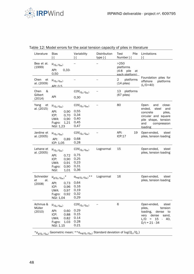
IRPWIND deliverable - project no. 609795
48
Table 12: Model errors for the axial tension capacity of piles in literature
Literature Bias
[-]
Variability
[-]
Distribution
type [-]
Test Pile
Number [-]
Limitations
[-]
Bea et al.
(1999) μ(Qc Qm⁄ )
API: 0,33-
0,50
-- -- >250
platforms
(4-8 pile at
each platform) Foundation piles for
offshore platforms
(L/D>40)
Chen et
al. (2009) μ(Qc Qm⁄ )
API: 0,5
-- -- 2 platforms
(14 piles)
Chen &
Gilbert
(2014)
API
COV(Qc Qm⁄ )
0,30
-- 13 platforms
(67 piles)
Yang et
al. (2015) μ(Qc Qm⁄ )
API: 0,90
ICP: 0,70
UWA: 0,90
Fugro: 1,21
NGI: 1,23
COV(Qc Qm⁄ )
0,55
0,34
0,40
0,45
0,47
-- 80 Open- and close-
ended, steel and
concrete piles,
circular and square
pile shape, tension
and compression
loading
Jardine et
al. (2005) μ(Qc Qm⁄ )
API: 0,89
ICP: 1,05
COV(Qc Qm⁄ )
0,68
0,28
-- API: 19
ICP:17
Open-ended, steel
piles, tension loading
Lehane et
al. (2005)
μ(Qc Qm⁄ )
API: 0,72
ICP: 0,90
UWA: 0,91
Fugro: 0,90
NGI: 1,01
COV(Qc Qm⁄ )
0,75
0,25
0,23
0,31
0,36
Lognormal 15 Open-ended, steel
piles, tension loading
Schneider
et al.
(2008)
μg(Qc Qm⁄ )*
API: 0,73
ICP: 0,96
UWA: 0,97
Fugro: 0,92
NGI: 1,04
σlog (Qc/Qm)**
0,64
0,16
0,19
0,32
0,29
Lognormal 16 Open-ended, steel
piles, tension loading
Achmus &
Müller
(2010)
μ(Qc Qm⁄ )
API: 0.60
ICP: 0.88
UWA: 0.82
Fugro: 1.03
NGI: 1.15
COV(Qc Qm⁄ )
0.29
0.15
0.14
0.28
0.21
-- 6 Open-ended, steel
piles, tension
loading, dense to
very dense sand,
L/D = 15 - 40,
D/t = 21 - 34
*μg(Qc Qm⁄ ) Geometric mean; **σlog (Qc/Qm) Standard deviation of log(Qc Qc⁄ )
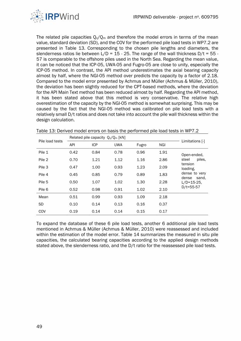
IRPWIND deliverable - project no. 609795
49
The related pile capacities Qc/Qm and therefore the model errors in terms of the mean
value, standard deviation (SD), and the COV for the performed pile load tests in WP7.2 are
presented in Table 13. Corresponding to the chosen pile lengths and diameters, the
slenderness ratios lie between L/D = 15 - 25. The range of the wall thickness D/t = 55 -
57 is comparable to the offshore piles used in the North Sea. Regarding the mean value,
it can be noticed that the ICP-05, UWA-05 and Fugro-05 are close to unity, especially the
ICP-05 method. In contrast, the API method underestimates the axial bearing capacity
almost by half, where the NGI-05 method over predicts the capacity by a factor of 2.18.
Compared to the model error presented by Achmus and Müller (Achmus & Müller, 2010),
the deviation has been slightly reduced for the CPT-based methods, where the deviation
for the API Main Text method has been reduced almost by half. Regarding the API method,
it has been stated above that this method is very conservative. The relative high
overestimation of the capacity by the NGI-05 method is somewhat surprising. This may be
caused by the fact that the NGI-05 method was calibrated on pile load tests with a
relatively small D/t ratios and does not take into account the pile wall thickness within the
design calculation.
Table 13: Derived model errors on basis the performed pile load tests in WP7.2
Pile load tests Related pile capacity Qc/Qm [kN]
Limitations [-] API ICP UWA Fugro NGI
Pile 1 0.42 0.84 0.78 0.96 1.91 Open-ended,
steel piles,
tension
loading,
dense to very
dense sand,
L/D=15-25,
D/t=55-57
Pile 2 0.70 1.21 1.12 1.16 2.86
Pile 3 0.47 1.00 0.93 1.23 2.09
Pile 4 0.45 0.85 0.79 0.89 1.83
Pile 5 0.50 1.07 1.02 1.30 2.28
Pile 6 0.52 0.98 0.91 1.02 2.10
Mean 0.51 0.99 0.93 1.09 2.18
SD 0.10 0.14 0.13 0.16 0.37
COV 0.19 0.14 0.14 0.15 0.17
To expand the database of these 6 pile load tests, another 6 additional pile load tests
mentioned in Achmus & Müller (Achmus & Müller, 2010) were reassessed and included
within the estimation of the model error. Table 14 summarizes the measured in situ pile
capacities, the calculated bearing capacities according to the applied design methods
stated above, the slenderness ratio, and the D/t ratio for the reassessed pile load tests.

IRPWIND deliverable - project no. 609795
50
Table 14: Comparison of measured and calculated pile bearing capacities for reassed pile
load tests from the literature
Pile load tests Measured pile
capacity [kN]
Calculated pile capacity [kN] Pile properties [1]
API ICP UWA Fugro NGI L/D D/t
EURIPIDES I 2900 2710 3834 3519 5061 4087 40.0 21.19
CLAROM CS 396 270.3 370.3 345.3 400.3 605.3 34.0 25.51
CLAROM CL 459 270.3 370.3 345.3 400.3 605.3 34.0 25.51
GOPAL R1 1450 1046 1007 848.7 845.7 1730 42.2 33.85
HOOGZAND I 830 129.1 648.1 671.1 732.1 808.1 19.7 22.25
HOOGZAND III 550 75.2 425.2 458.2 604.2 517.2 14.9 22.25
Table 15 provides all related pile capacities Qc/Qm of the considered pile load tests from
WP7.2 and the reassessed pile load tests given in Table 14. In addition, the statistics for
the so obtained model errors are specified. The slenderness ratio and the D/t ratio differ
considerably. Nevertheless, these ratios are relevant to industry practice. Since the NGI-
05 method obviously does not capture the capacity of the tested piles as described above,
only the reassessed pile load tests were considered.
Table 15: Model errors on basis performed pile load tests in WP7.2 and reassessed pile
load tests
Pile load tests Related pile capacity Qc/Qm [kN]
Limitations [-] API ICP UWA Fugro NGI*
Pile 1 0.42 0.84 0.78 0.96 -
Open-ended,
steel piles,
tension
loading,
dense to very
dense sand,
L/D=15-40,
D/t=21-57
Pile 2 0.70 1.21 1.12 1.16 -
Pile 3 0.47 1.00 0.93 1.23 -
Pile 4 0.45 0.85 0.79 0.89 -
Pile 5 0.50 1.07 1.02 1.30 -
Pile 6 0.52 0.98 0.91 1.02 -
EURIPIDES I 0.93 1.32 1.21 1.75 1.41
CLAROM CS 0.68 0.94 0.87 1.01 1.53
CLAROM CL 0.59 0.81 0.75 0.87 1.32
GOPAL R1 0.72 0.69 0.59 0.58 1.19
HOOGZAND I 0.16 0.78 0.81 0.88 0.97
HOOGZAND III 0.14 0.77 0.83 1.10 0.94
Mean 0.52 0.94 0.89 1.06 1.23
SD 0.23 0.19 0.17 0.29 0.24
COV 0.44 0.20 0.19 0.27 0.19
* Only reassessed pile load tests from Achmus & Müller (2010) are considered
As it can be seen, the mean value has been slightly reduced for the ICP-05, UWA-05, and
Fugro-05 method compared to the model error related to the tested piles. The mean value
for the API method has not been significantly changed. Regarding the deviation, an
increase can be noticed in all cases. For the reassessed NGI-05 method, only the mean
value has been increased, whereas the deviation is almost the same. Altogether, the ICP-
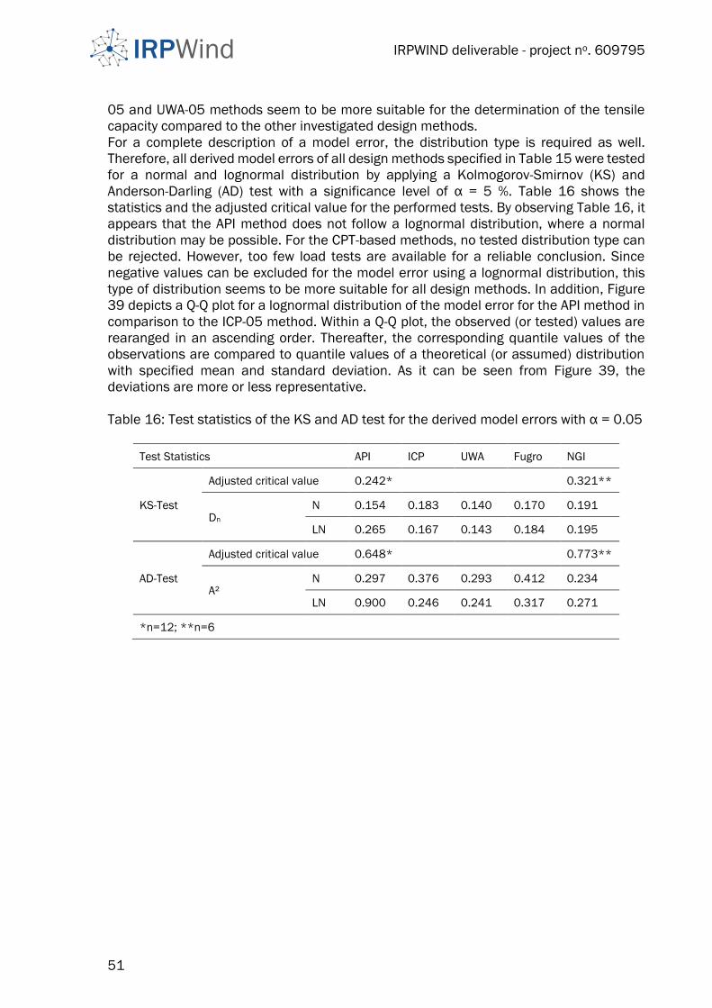
IRPWIND deliverable - project no. 609795
51
05 and UWA-05 methods seem to be more suitable for the determination of the tensile
capacity compared to the other investigated design methods.
For a complete description of a model error, the distribution type is required as well.
Therefore, all derived model errors of all design methods specified in Table 15 were tested
for a normal and lognormal distribution by applying a Kolmogorov-Smirnov (KS) and
Anderson-Darling (AD) test with a significance level of α = 5 %. Table 16 shows the
statistics and the adjusted critical value for the performed tests. By observing Table 16, it
appears that the API method does not follow a lognormal distribution, where a normal
distribution may be possible. For the CPT-based methods, no tested distribution type can
be rejected. However, too few load tests are available for a reliable conclusion. Since
negative values can be excluded for the model error using a lognormal distribution, this
type of distribution seems to be more suitable for all design methods. In addition, Figure
39 depicts a Q-Q plot for a lognormal distribution of the model error for the API method in
comparison to the ICP-05 method. Within a Q-Q plot, the observed (or tested) values are
rearanged in an ascending order. Thereafter, the corresponding quantile values of the
observations are compared to quantile values of a theoretical (or assumed) distribution
with specified mean and standard deviation. As it can be seen from Figure 39, the
deviations are more or less representative.
Table 16: Test statistics of the KS and AD test for the derived model errors with α = 0.05
Test Statistics API ICP UWA Fugro NGI
KS-Test
Adjusted critical value 0.242* 0.321**
Dn N 0.154 0.183 0.140 0.170 0.191
LN 0.265 0.167 0.143 0.184 0.195
AD-Test
Adjusted critical value 0.648* 0.773**
A² N 0.297 0.376 0.293 0.412 0.234
LN 0.900 0.246 0.241 0.317 0.271
*n=12; **n=6

IRPWIND deliverable - project no. 609795
52
Figure 39: Q-Q plot for a lognormal distribution of the model error for the API method and
the ICP-05 method
3.1.3 Assesment of design methods
3.1.3.1 Pile-Soil System under consideration
For the performed study, typical site conditions for the North Sea and typical ranges for
the foundation pile properties are assumed.
Since the subsoil in the German North Sea mostly consists of dense sands with only
limited intermediate cohesive layers, two idealized CPT profiles for homogeneous dense
(Dr = 0.75) and very dense (Dr = 0.90) sands were considered, where the mean value of
the grain size at 50 % of the grain size distribution was chosen to μD50 = 0.4 mm. The
mean value of the effective unit weight was assumed to be μγ’ = 10 kN/m³ in both cases,
since this value represents a reasonable estimate for both soil densities.
The choice of pile properties depends on the type of support structure for the wind turbine,
the water depth, and the subsoil condition at the desired location. In general, it can be
said that pile slenderness ratios between L/D = 15 and L/D = 40 are used for jacket
support structures of offshore wind turbines. Thereby, the pile outer diameter is varying
between D = 1 m and D = 3 m, where the pile embedded length is commonly chosen to
be between L = 20 m and L = 60 m. The regular pile wall thickness which is mostly used
can approximately be determined by t = D/50. Figure 40 shows the considered pile
properties and soil conditions.
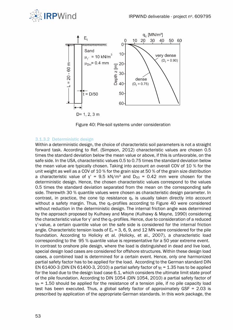
IRPWIND deliverable - project no. 609795
53
Figure 40: Pile-soil systems under consideration
3.1.3.2 Deterministic design
Within a deterministic design, the choice of characteristic soil parameters is not a straight
forward task. According to Ref. (Simpson, 2012) characteristic values are chosen 0.5
times the standard deviation below the mean value or above, if this is unfavorable, on the
safe side. In the USA, characteristic values 0.5 to 0.75 times the standard deviation below
the mean value are typically chosen. Taking into account an overall COV of 10 % for the
unit weight as well as a COV of 10 % for the grain size at 50 % of the grain size distribution
a characteristic value of γ’ = 9.5 kN/m³ and D50 = 0.42 mm were chosen for the
deterministic design. Hence, the chosen characteristic values correspond to the values
0.5 times the standard deviation separated from the mean on the corresponding safe
side. Therewith 30 % quantile values were chosen as characteristic design parameter. In
contrast, in practice, the cone tip resistance qc is usually taken directly into account
without a safety margin. Thus, the qc-profiles according to Figure 40 were considered
without reduction in the deterministic design. The internal friction angle was determined
by the approach proposed by Kulhawy and Mayne (Kulhawy & Mayne, 1990) considering
the characteristic value for γ’ and the qc-profiles. Hence, due to consideration of a reduced
γ’-value, a certain quantile value on the safe side is considered for the internal friction
angle. Characteristic tension loads of Ec = 3, 6, 9, and 12 MN were considered for the pile
foundation. According to Holicky et al. (Holicky, et al., 2007), a characteristic load
corresponding to the 95 % quantile value is representative for a 50 year extreme event.
In contrast to onshore pile design, where the load is distinguished in dead and live load,
special design load cases are considered for offshore structures. Within these design load
cases, a combined load is determined for a certain event. Hence, only one harmonized
partial safety factor has to be applied for the load. According to the German standard DIN
EN 61400-3 (DIN EN 61400-3, 2010) a partial safety factor of γE = 1.35 has to be applied
for the load due to the design load case 6.1, which considers the ultimate limit state proof
of the pile foundation. According to DIN 1054 (DIN 1054, 2010) a partial safety factor of
γR = 1.50 should be applied for the resistance of a tension pile, if no pile capacity load
test has been executed. Thus, a global safety factor of approximately GSF = 2.03 is
prescribed by application of the appropriate German standards. In this work package, the
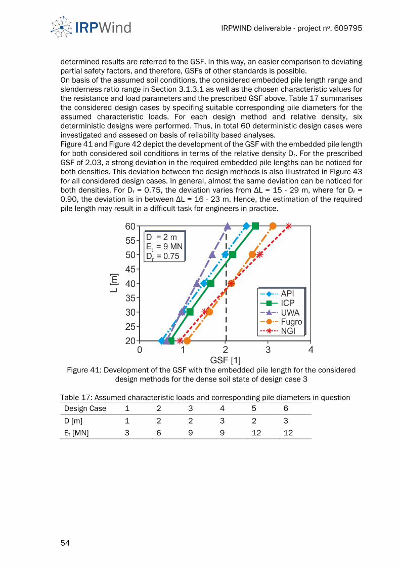
IRPWIND deliverable - project no. 609795
54
determined results are referred to the GSF. In this way, an easier comparison to deviating
partial safety factors, and therefore, GSFs of other standards is possible.
On basis of the assumed soil conditions, the considered embedded pile length range and
slenderness ratio range in Section 3.1.3.1 as well as the chosen characteristic values for
the resistance and load parameters and the prescribed GSF above, Table 17 summarises
the considered design cases by specifing suitable corresponding pile diameters for the
assumed characteristic loads. For each design method and relative density, six
deterministic designs were performed. Thus, in total 60 deterministic design cases were
investigated and assesed on basis of reliability based analyses.
Figure 41 and Figure 42 depict the development of the GSF with the embedded pile length
for both considered soil conditions in terms of the relative density Dr. For the prescribed
GSF of 2.03, a strong deviation in the required embedded pile lengths can be noticed for
both densities. This deviation between the design methods is also illustrated in Figure 43
for all considered design cases. In general, almost the same deviation can be noticed for
both densities. For Dr = 0.75, the deviation varies from ΔL = 15 - 29 m, where for Dr =
0.90, the deviation is in between ΔL = 16 - 23 m. Hence, the estimation of the required
pile length may result in a difficult task for engineers in practice.
Figure 41: Development of the GSF with the embedded pile length for the considered
design methods for the dense soil state of design case 3
Table 17: Assumed characteristic loads and corresponding pile diameters in question
Design Case 1 2 3 4 5 6
D [m] 1 2 2 3 2 3
Et [MN] 3 6 9 9 12 12
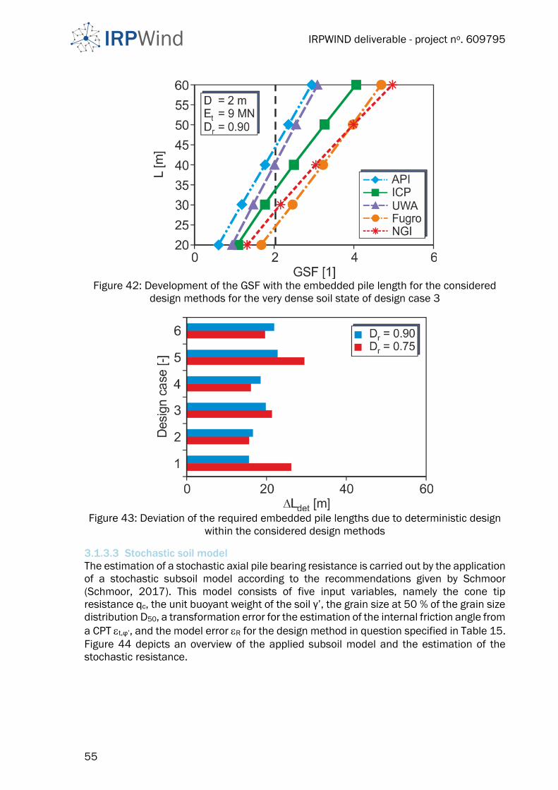
IRPWIND deliverable - project no. 609795
55
Figure 42: Development of the GSF with the embedded pile length for the considered
design methods for the very dense soil state of design case 3
Figure 43: Deviation of the required embedded pile lengths due to deterministic design
within the considered design methods
3.1.3.3 Stochastic soil model
The estimation of a stochastic axial pile bearing resistance is carried out by the application
of a stochastic subsoil model according to the recommendations given by Schmoor
(Schmoor, 2017). This model consists of five input variables, namely the cone tip
resistance qc, the unit buoyant weight of the soil γ’, the grain size at 50 % of the grain size
distribution D50, a transformation error for the estimation of the internal friction angle from
a CPT t,ϕ’, and the model error R for the design method in question specified in Table 15.
Figure 44 depicts an overview of the applied subsoil model and the estimation of the
stochastic resistance.
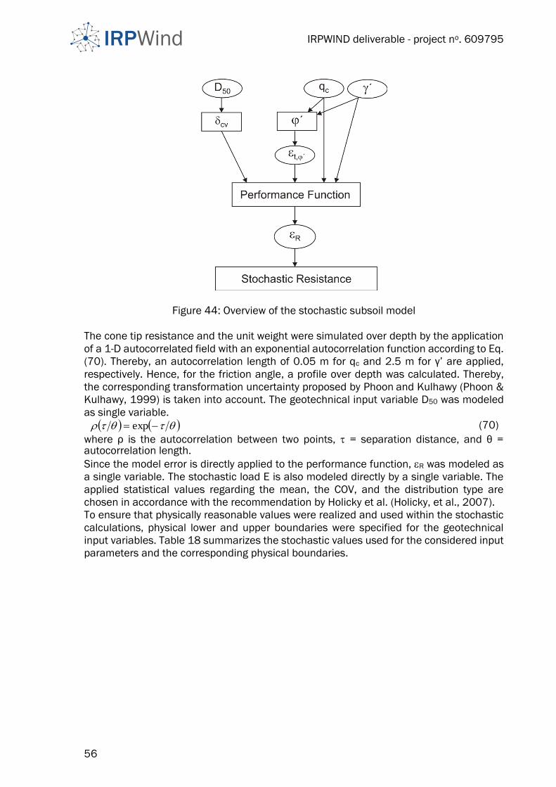
IRPWIND deliverable - project no. 609795
56
Figure 44: Overview of the stochastic subsoil model
The cone tip resistance and the unit weight were simulated over depth by the application
of a 1-D autocorrelated field with an exponential autocorrelation function according to Eq.
(70). Thereby, an autocorrelation length of 0.05 m for qc and 2.5 m for γ’ are applied,
respectively. Hence, for the friction angle, a profile over depth was calculated. Thereby,
the corresponding transformation uncertainty proposed by Phoon and Kulhawy (Phoon &
Kulhawy, 1999) is taken into account. The geotechnical input variable D50 was modeled
as single variable.
exp (70)
where ρ is the autocorrelation between two points, = separation distance, and θ = autocorrelation length.
Since the model error is directly applied to the performance function, R was modeled as
a single variable. The stochastic load E is also modeled directly by a single variable. The
applied statistical values regarding the mean, the COV, and the distribution type are
chosen in accordance with the recommendation by Holicky et al. (Holicky, et al., 2007).
To ensure that physically reasonable values were realized and used within the stochastic
calculations, physical lower and upper boundaries were specified for the geotechnical
input variables. Table 18 summarizes the stochastic values used for the considered input
parameters and the corresponding physical boundaries.
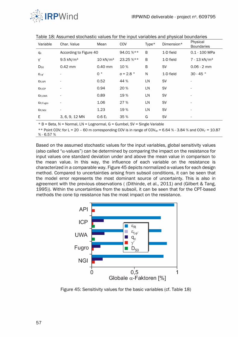
IRPWIND deliverable - project no. 609795
57
Table 18: Assumed stochastic values for the input variables and physical boundaries
Variable Char. Value Mean COV Type* Dimension* Physical
Boundaries
qc According to Figure 40 94.01 %** B 1-D field 0.1 - 100 MPa
γ' 9.5 kN/m³ 10 kN/m³ 23.25 %** B 1-D field 7 - 13 kN/m³
D50 0.42 mm 0.40 mm 10 % B SV 0.06 - 2 mm
εt,ϕ’ - 0 ° σ = 2.8 ° N 1-D field 30 - 45 °
εR,API - 0.52 44 % LN SV -
εR,ICP - 0.94 20 % LN SV -
εR,UWA - 0.89 19 % LN SV -
εR,Fugro - 1.06 27 % LN SV -
εR,NGI - 1.23 19 % LN SV -
E 3, 6, 9, 12 MN 0.6 Et 35 % G SV -
* B = Beta, N = Normal, LN = Lognormal, G = Gumbel, SV = Single Variable
** Point COV; for L = 20 – 60 m corresponding COV is in range of COVqc = 6.64 % - 3.84 % and COVγ’ = 10.87
% - 6.57 %
Based on the assumed stochastic values for the input variables, global sensitivity values
(also called “-values”) can be determined by comparing the impact on the resistance for
input values one standard deviation under and above the mean value in comparison to
the mean value. In this way, the influence of each variable on the resistance is
characterized in a comparable way. Figure 45 depicts normalized α-values for each design
method. Compared to uncertainties arising from subsoil conditions, it can be seen that
the model error represents the most dominant source of uncertainty. This is also in
agreement with the previous observations ( (Dithinde, et al., 2011) and (Gilbert & Tang,
1995)). Within the uncertainties from the subsoil, it can be seen that for the CPT-based
methods the cone tip resistance has the most impact on the resistance.
Figure 45: Sensitivity values for the basic variables (cf. Table 18)

IRPWIND deliverable - project no. 609795
58
3.1.3.4 Reliability based design
On basis of the described stochastic subsoil model and loading condition in Section
3.1.3.3, a Monte Carlo Simulation with 6 Million realizations for each of the 60 design
cases was executed. Thereby, the pile embedded length was varied and the pile length
corresponding to the reliability index β = 3.8 required for a ULS design according to
Eurocode 0 (Eurocode 0, 2010) was sought. Figure 46 and Figure 47 depict the calculated
reliability index over the embedded pile length for both densities, where design case 3 is
shown for all considered design methods. For both densities, still, a deviation regarding
the required embedded pile length can be noticed with respect to the deterministic deign.
For the same reliability index of β = 3.8, it can be seen that the API-method leads to a
required pile length of 53 m, where the ICP-method leads to a pile length of 33 m in case
of Dr = 0.90. However, it is obvious that a longer pile has a higher bearing resistance, and
therefore, a lower failure probability. Since the real bearing capacity and the variation for
the subsoil parameters, and therefore, the real curve of the reliability index over depth is
unknown, Figure 46 and Figure 47 should be interpreted that in case of Dr = 0.90 for β =
3.8 the embedded pile length should be in a range between approximately 33 – 53 m.
However, since the model error for the API-method indicates a much higher COV in
comparison to the CPT-based design methods, the results of the API-method are not taken
into account for further evaluation. In this way, the API-method is considered as not
reliable as the CPT-based methods.
Figure 46: Calculated reliability Index over the embedded pile length with Dr = 0.75 for
design case 3

IRPWIND deliverable - project no. 609795
59
Figure 47: Calculated reliability Index over the embedded pile length with Dr = 0.90 for
design case 3
3.1.3.5 Comparison of deterministic and reliability based design
Figure 48 elucidates the deviation within the different design methods in the required
embedded pile length of the reliability based results only for the CPT-based design
methods in relation to the deterministic based results for the 6 considered design cases.
For the design cases 2 to 6, almost half the deviation with respect to the deterministic
design can be seen for the reliability based design, where for design case 1, a lower
deviation can be noticed. However, it should be emphasized that the deviations for the
embedded pile length due to the deterministic design result from 5 design methods,
where the deviations due to reliability based design result only from the 4 CPT-based
design methods. In the same way, Figure 49 shows the mean required embedded pile
length of all design methods due to a reliability based design in relation to the
deterministic design. Hence, for both densities a slightly increase of the piles embedded
length is required in comparison to the deterministic approach.

IRPWIND deliverable - project no. 609795
60
Figure 48: Deviation in the required embedded pile length for the reliability based
designs only of the CPT-based methods in comparison to deterministic designs
Figure 49: Comparison of the mean required embedded pile length L due to reliability
based designs only of the CPT-based methods and deterministic designs
3.1.3.6 Evaluation of design methods
A new calibration approach, where the minimum and maximum embedded pile lengths of
all design methods, except the API-method, are considered as the upper and lower
boundaries for a corresponding reliability index is investigated. Within this assumption,
the mean value of the required embedded pile length is assumed as the most likely
outcome within this range for all design cases. Thus, an integration of all CPT-based design
methods and model errors is executed. In that way, an indirect increase of the assumed
database for the model error is done. From the relationship between the deterministic
design and the embedded pile length (see Figure 46 and Figure 47) the corresponding
GSF can be obtained for the assumed lower and upper bound as well as for the mean
required embedded pile length. Table 19 summarizes the required GSFs for each design
method according to the new introduced approach. By dividing the GSF by the partial
safety factor for the load, again the corresponding partial safety factor for the resistance
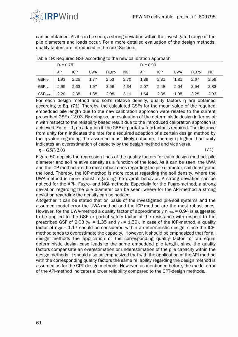
IRPWIND deliverable - project no. 609795
61
can be obtained. As it can be seen, a strong deviation within the investigated range of the
pile diameters and loads occur. For a more detailed evaluation of the design methods,
quality factors are introduced in the next Section.
Table 19: Required GSF according to the new calibration approach
Dr = 0.75 Dr = 0.90
API ICP UWA Fugro NGI API ICP UWA Fugro NGI
GSFmin 1.93 2.25 1.77 2.53 2.70 1.39 2.31 1.81 2.67 2.59
GSFmax 2.95 2.63 1.97 3.59 4.34 2.07 2.48 2.04 3.94 3.83
GSFmean 2.20 2.38 1.88 2.98 3.11 1.64 2.38 1.95 3.28 2.93
For each design method and soil’s relative density, quality factors η are obtained
according to Eq. (71). Thereby, the calculated GSFs for the mean value of the required
embedded pile length due to the new calibration approach were related to the current
prescribed GSF of 2.03. By doing so, an evaluation of the deterministic design in terms of
η with respect to the reliability based result due to the introduced calibration approach is
achieved. For η = 1, no adaption if the GSF or partial safety factor is required. The distance
from unity for η indicates the rate for a required adaption of a certain design method by
the η-value regarding the assumed most likely outcome. Thereby η higher than unity
indicates an overestimation of capacity by the design method and vice versa.
03.2GSF (71)
Figure 50 depicts the regression lines of the quality factors for each design method, pile
diameter and soil relative density as a function of the load. As it can be seen, the UWA
and the ICP-method are the most robust ones regarding the pile diameter, soil density and
the load. Thereby, the ICP-method is more robust regarding the soil density, where the
UWA-method is more robust regarding the overall behavior. A strong deviation can be
noticed for the API-, Fugro- and NGI-methods. Especially for the Fugro-method, a strong
deviation regarding the pile diameter can be seen, where for the API-method a strong
deviation regarding the density can be noticed.
Altogether it can be stated that on basis of the investigated pile-soil systems and the
assumed model error the UWA-method and the ICP-method are the most robust ones.
However, for the UWA-method a quality factor of approximately ηUWA = 0.94 is suggested
to be applied to the GSF or partial safety factor of the resistance with respect to the
prescribed GSF of 2.03 (γE = 1.35 and γR = 1.50). In case of the ICP-method, a quality
factor of ηICP = 1.17 should be considered within a deterministic design, since the ICP-
method tends to overestimate the capacity. However, it should be emphasized that for all
design methods the application of the corresponding quality factor for an equal
deterministic design case leads to the same embedded pile length, since the quality
factors compensate an overestimation or underestimation of the pile capacity within the
design methods. It should also be emphasized that with the application of the API-method
with the corresponding quality factors the same reliability regarding the design method is
assumed as for the CPT-design methods. However, as mentioned before, the model error
of the API-method indicates a lower reliability compared to the CPT-design methods.
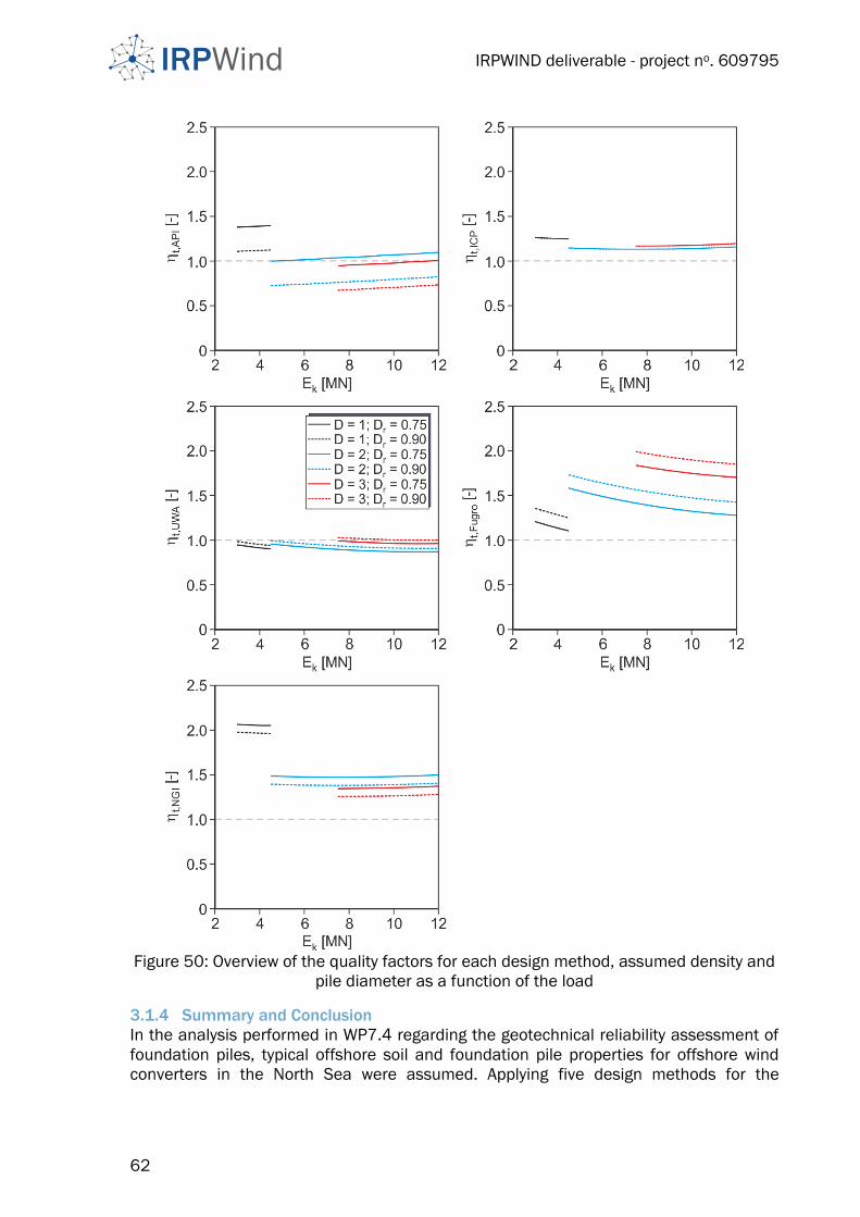
IRPWIND deliverable - project no. 609795
62
Figure 50: Overview of the quality factors for each design method, assumed density and
pile diameter as a function of the load
3.1.4 Summary and Conclusion
In the analysis performed in WP7.4 regarding the geotechnical reliability assessment of
foundation piles, typical offshore soil and foundation pile properties for offshore wind
converters in the North Sea were assumed. Applying five design methods for the
IRPWIND deliverable - project no. 609795
63
determination of the axial tensile resistance, namely the API-, ICP-, UWA-, Fugro- and NGI-
methods, in total 60 deterministic valid designs were evaluated within a reliability based
design. By taking into account typical variability for the assumed soil condition as well as
the determined model error for the investigated design methods, a reliability based
determination of the failure probability in terms of the reliability index was executed.
Further, a new calibration approach regarding the required GSF for the prescribed failure
probability was introduced. Thereby, the results due to the reliability based calculations of
all design methods were taken into account. Furthermore, quality factors were derived for
each design method as function of the load, pile diameter, and soil density. On basis of
these quality factors, a more sophisticated evaluation of both, the considered design
method as well as the safety level in terms of the required GSF (or partial safety factor) is
possible. By applying the quality factors, a more robust result within a deterministic design
regarding the embedded pile length is achieved. Based on the investigated pile-soil
systems and the assumed model error the calculated quality factors indicate that the
UWA- and ICP-method are the most robust design methods in comparison to the other
investigated offshore design methods. By applying the UWA-method, a decrease in the
GSF or the resistance partial safety factor of approximately 0.94 with respect to the
prescribed GSF of 2.03 should be considered, where for the ICP-method an increase of
1.17 of the GSF should be taken into account within a deterministic design.
IRPWIND deliverable - project no. 609795
64
3.2 Reliability of the substructure under consideration of the turbine and soil
parameters The second part of the work on reliability of piles and substructures under consideration
of soil parameters in WP7.4, described in this section, concentrates on the probabilistic
design of offshore substructures. However, due to the complex interaction between
turbine, substructure, and foundation, it is presumed that a decoupled consideration is
not sufficient for a sophisticated reliability analysis. Therefore, in this section, fully coupled
aero-elastic simulations using the simulation code FASTv8 (Jonkman, 2013) are
conducted taking into account the substructure, the turbine, and an adequate soil model.
In this context, the consideration of the soil is regarded to be essential - although
nowadays the soil-structure interaction is frequently neglected (e.g. (Jonkman, et al.,
2012) or (Zwick & Muskulus, 2015)) - as soil parameters exhibit a high amount of
uncertainty. Furthermore, in D72.2 of the IRPWind project, new data concerning soil-
structure interaction was gained, which is in the current context.
Therefore, the general idea of this part of the project is to conduct probabilistic simulations
of offshore wind turbines using a fully coupled aero-elastic model to evaluate the reliability
of offshore wind turbine support structures. This approach gives a first insight in the
difference of probabilistic and deterministic designs, demonstrates the potential of
probabilistic simulations and creates a basis for further studies focusing on safety factor
(SF) calibration. SF calibration and different designs for deterministic and probabilistic
approaches (i.e. a classic and a robust optimization) are out of the scope of the current
work, but can be based on the present findings.
3.2.1 Introduction and concept
As stated before, probabilistic simulations for fully coupled offshore wind turbines
including an adequate soil model are desired. To achieve this aim, there are several
challenges to be handled. Firstly, an adequate soil model for probabilistic simulations has
to be developed. Current soil models are either rudimentary (e.g. apparent fixity length
(Zaaijer, 2006)) or numerically expensive (e.g. FE or p-y models (Thieken, et al., 2015)).
Furthermore, state-of-the-art models, like p-y curves, do not match experimental results
(Hald, et al., 2009), and therefore, have high model errors. Secondly, for many
probabilistic parameters, the statistical distributions are unknown. And lastly, the fatigue
damage calculation, being decisive for the substructure lifetime assessment, is very CPU
intensive and exhibits high uncertainties (Zwick & Muskulus, 2015).
Therefore, in this project, the following steps are conducted to solve these problems and
to enable probabilistic calculations for coupled time domain models of offshore wind
turbines. The conducted steps correspond to the structure of the rest of section 3.2, which
is concluded with a summary and an outlook:
• Development of a soil model that does not increase the computing time
significantly, but includes operating point dependent stiffnesses and can be
combined with substructural reduction schemes like the Craig-Bampton reduction
(Craig Jr. & Bampton, 1968).
• Assessment of the importance of soil models for the overall turbine behavior and
of the differences between various p-y models to identify those models that are
adequate for coupled dynamics.
• Evaluation of various p-y models using the experimental data of WP7.2.

IRPWIND deliverable - project no. 609795
65
• Deviation of statistical distributions for important environmental conditions based
on offshore measurement data (FINO project 1) and literature values (e.g. (Zaaijer,
2006) or (Hansen, et al., 2015)).
• Global sensitivity analysis to identify those parameters that have to be treated
probabilistically and those that can be fixed to deterministic values.
• Definition of a deterministic and a probabilistic simulation model. Here, the
structural design is the same, as an independent optimization of the deterministic
and the probabilistic design would be far out of the scope of this project. However,
the offshore conditions (e.g. wind speeds, wave heights, etc.) differ, as they are
either set deterministic values or follow statistical distributions.
• Calculation of the damage distribution (wind speed versus fatigue lifetime damage)
and the uncertainty in the lifetime damage approximation. Comparison of
deterministic and probabilistic damages.
3.2.2 Wind turbine model
In order to simulate offshore wind turbines using probabilistic methods, an adequate wind
turbine model has to be used. This model has to be accurate enough for the present
application. However, at the same time, the computing time has to be low enough to
manage the high amount of required simulations of a probabilistic approach. Additionally,
the model has to include all significant parameters that shall be varied. Therefore, this
section gives a short introduction in the overall time domain model being used.
Subsequently, an approach to consider soil properties in probabilistic transient
simulations is proposed. This approach is based on different soil models. Finally, data of
WP7.2 is used to assess the soil-structure interaction models being the basis of the
proposed approach of soil consideration.
3.2.2.1 Time domain model
Offshore wind turbines are highly dynamic structures with changing external loads (for
example loads resulting from turbulent wind or irregular waves) even in otherwise
deterministic simulations (i.e. deterministic simulations are already partly stochastic).
Therefore, transient simulations are necessary to model dynamic effects accurately. This
is why current standards and guidelines (e.g. (International Electrotechnical Commision,
2009)) demand holistic time domain simulations for the design and certification process
of offshore wind turbines. There are several simulation codes being capable of conducting
these time domain simulations, for example Bladed, FAST, and HAWC2, to mention a few.
Studies showed that the results of these codes are mainly comparable ( (Jonkman, et al.,
2012) , (Jonkman & Musial, 2010)). Hence, all of them can be chosen to be used as the
basic simulation tool in this work package. As FAST is open source and can be adjusted
and expanded easily, for example by additional soil models, it is utilized here. FAST offers
up to 23 degrees of freedom (DoF) for a land based turbine, including nine for the rotor
blades (three for each blade), four for rotor-teeter motion, drivetrain, generator, and yaw
rotation and ten for tower bending and platform movements. This limited number of DoF
reduces the computing time to an adequate level. So, FAST is capable of conducting
probabilistic simulations with a great number of computations. However, the
consideration of offshore substructures in the model is complicated. Substructures are
normally modelled using FE methods with beam elements having thousands degrees of
freedom. Therefore, a reduction method, based on the work of Craig and Bampton (Craig
1 Research platforms in the North Sea and Baltic Sea funded under the German Federal Ministry for Economic Affairs and Energy and
“Projektträger Jülich” (http://www.fino-offshore.de/en)

IRPWIND deliverable - project no. 609795
66
Jr. & Bampton, 1968) and called Component-Mode-Synthesis, is implemented in FAST.
This reduction method allows a modal representation of the substructure with about five
to 15 degrees of freedom (Damiani, et al., 2013). Nonetheless, this reduction approach
has the significant shortcoming that classical soil models, based on nonlinear springs
distributed along the piles, cannot be applied. Thence, in FAST the substructure is
assumed clamped to the seabed. Since variations of soil parameters in probabilistic
analyses can affect the overall turbine behavior significantly, a different approach of
taking the soil into account has to be implemented. This approach is presented in the next
section.
3.2.2.2 Soil model for transient calculations
Probabilistic transient wind turbine simulations need to have manageable computing
times. This is why current holistic simulation tools are based on reduction schemes to limit
the number of degrees of freedom used for the substructure. A classical soil model based
on p-y curves and T-z curves has, firstly, too many degrees of freedom to be efficiently
used, and secondly, it cannot be included in a reduction scheme like the Component-
Mode-Synthesis of Craig and Bampton (Craig Jr. & Bampton, 1968). Hence, a two-step
approach for an effective consideration of soil characteristics in transient simulations was
developed. This approach does not add necessarily DoFs to the structural model of the
substructure. It was introduced as part of this project in (Häfele, et al., 2016) and refined
in (Hübler, et al., 2016) and (Hübler, et al., 2018).
In this section, a short introduction in this method is presented and the most important
results are given. For more details, it is referred to (Häfele, et al., 2016), (Hübler, et al.,
2016) and (Hübler, et al., 2018). As the approach can be based on different p-y and T-z
soil models, some of these models are introduced as well.
To understand the present approach, firstly, the reduction scheme of FAST is explained. It
is assumed that the structural assembly of the substructure was derived in the following
form, for example as the result of a FE discretization:
𝑴 + 𝑪 + 𝑲 = 𝐹 . (72)
M is the mass matrix in this equation, C the damping matrix, K the stiffness matrix, the
displacement vector along all degrees of freedom and 𝐹 comprises the corresponding
external forces. Dots represent time derivatives.
In addition, the vector is partitioned into the so called vectors of boundary
displacements 𝑅 and interior displacements 𝐿 in the following way:
= ( 𝑅
𝐿). (73)
Therefore, Eq. (72) can be written as:
(𝑴𝑅𝑅 𝑴𝑅𝐿
𝑴𝐿𝑅 𝑴𝐿𝐿) ( 𝑅
𝐿) + (
𝑪𝑅𝑅 𝑪𝑅𝐿𝑪𝐿𝑅 𝑪𝐿𝐿
) ( 𝑅
𝐿) + (
𝑲𝑅𝑅 𝑲𝑅𝐿𝑲𝐿𝑅 𝑲𝐿𝐿
) ( 𝑅
𝐿) = (
𝐹 𝑅
𝐹 𝐿). (74)
If no boundary conditions are applied, the stiffness matrix K is singular due to rigid body
motions. This is why, in the original FAST simulation tool, boundary conditions are applied
and the substructure is fixed at the seabed ( 𝑏𝑎𝑠𝑒 = 0). This means:
𝑅 = ( 𝑖𝑛𝑡
𝑏𝑎𝑠𝑒), (75)
where 𝑖𝑛𝑡 is the vector of the displacements at interface nodes between tower and
substructure. 𝑏𝑎𝑠𝑒 is the vector of the displacements at the bottom of the structure

IRPWIND deliverable - project no. 609795
67
(mudline). This approach is changed here, so that only the interface nodes are boundary
nodes and the base nodes are part of the interior nodes:
𝑅 = 𝑖𝑛𝑡 (76)
and
𝐿 = ( 𝐼
𝑏𝑎𝑠𝑒). (77)
It follows:
𝑴𝐿𝐿 = (𝑴𝐼 𝑴𝐼,𝑏𝑎𝑠𝑒
𝑴𝑏𝑎𝑠𝑒,𝐼 𝑴𝑏𝑎𝑠𝑒) (78)
and
𝑲𝐿𝐿 = (𝑲𝐼 𝑲𝐼,𝑏𝑎𝑠𝑒
𝑲𝑏𝑎𝑠𝑒,𝐼 𝑲𝑏𝑎𝑠𝑒). (79)
The stiffness matrix is still singular, as the boundary conditions are not applied anymore
( 𝑏𝑎𝑠𝑒 ≠ 0). Hence, the matrices 𝑴𝑏𝑎𝑠𝑒 and 𝑲𝑏𝑎𝑠𝑒 containing the terms of the structural
system assembly are changed according to Eqs (80) and (81) by adding n stiffness (𝑲𝑠𝑜𝑖𝑙,𝑖) and mass matrices (𝑴𝑠𝑜𝑖𝑙,𝑖) on the main diagonal:
𝑴𝑏𝑎𝑠𝑒∗ = (
𝑴𝑏𝑎𝑠𝑒,11 +𝑴𝑠𝑜𝑖𝑙,1 ⋯ 𝑴𝑏𝑎𝑠𝑒,1𝑛
⋮ ⋱ ⋮𝑴𝑏𝑎𝑠𝑒,𝑛1 ⋯ 𝑴𝑏𝑎𝑠𝑒,𝑛𝑛 +𝑴𝑠𝑜𝑖𝑙,𝑛
), (80)
𝑲𝑏𝑎𝑠𝑒∗ = (
𝑲𝑏𝑎𝑠𝑒,11 +𝑲𝑠𝑜𝑖𝑙,1 ⋯ 𝑲𝑏𝑎𝑠𝑒,1𝑛⋮ ⋱ ⋮
𝑲𝑏𝑎𝑠𝑒,𝑛1 ⋯ 𝑲𝑏𝑎𝑠𝑒,𝑛𝑛 +𝑲𝑠𝑜𝑖𝑙,𝑛
). (81)
This removes the singularity of K and it follows:
(𝑴𝑅𝑅 𝑴𝑅𝐿
𝑴𝐿𝑅 𝑴𝐿𝐿∗ ) (
𝑅
𝐿) + (
𝑪𝑅𝑅 𝑪𝑅𝐿𝑪𝐿𝑅 𝑪𝐿𝐿
) ( 𝑅
𝐿) + (
𝑲𝑅𝑅 𝑲𝑅𝐿𝑲𝐿𝑅 𝑲𝐿𝐿
∗ ) ( 𝑅
𝐿) = (
𝐹 𝑅
𝐹 𝐿), (82)
with
𝑴𝐿𝐿∗ = (
𝑴𝐼 𝑴𝐼,𝑏𝑎𝑠𝑒
𝑴𝑏𝑎𝑠𝑒,𝐼 𝑴𝑏𝑎𝑠𝑒∗ ) (83)
and
𝑲𝐿𝐿∗ = (
𝑲𝐼 𝑲𝐼,𝑏𝑎𝑠𝑒𝑲𝑏𝑎𝑠𝑒,𝐼 𝑲𝑏𝑎𝑠𝑒
∗ ). (84)
Up to here, the number of degrees of freedom was not reduced and it is still the same as
for the FE discretization. To reduce the size of 𝐿, a Ritz transformation is applied and the
number of DoFs is reduced to m generalized interior coordinates (𝑞 𝑚). As the boundary
displacements 𝑅 are not affected by the Component-Mode-Synthesis, it follows:
( 𝑅
𝐿) = 𝜱(
𝑅
𝑞 𝑚), (85)
with
IRPWIND deliverable - project no. 609795
68
𝜱 = (𝑰 𝟎𝜱𝑅 𝜱𝐿
), (86)
where 𝜱𝑅 are the constraint modes, 𝜱𝐿 are the fixed-interface normal modes, 𝑰 is the
identity matrix, and 𝟎 is the zero matrix.
The constraint modes 𝜱𝑅 can be easily calculated by using Eq. (82), when the
homogenous, static case of the rigid body is considered and all boundary DoFs are set to
unit displacement. Eq. (82) simplifies to:
(𝑲𝑅𝑅 𝑲𝑅𝐿𝑲𝐿𝑅 𝑲𝐿𝐿
∗ ) (𝐼
0 ) = (0
0 ) (87)
and it follows:
𝜱𝑅 = −𝑲𝐿𝐿∗−1𝑲𝐿𝑅. (88)
The matrix of the fixed-interface normal modes 𝜱𝐿 compromises the first m eigenvectors
of the eigenvalue problem:
𝑲𝐿𝐿∗ 𝜱𝐿 = Ω𝑳
𝟐𝑴𝐿𝐿∗ 𝜱𝐿 . (89)
With 𝜱𝑚 being the truncated subset of 𝜱𝐿 and Eq. (82), the Ritz transformation leads to:
(𝑴𝐵𝐵 𝑴𝐵𝑚
𝑴𝑚𝐵 𝑰) ( 𝑅
𝑚) + (
𝟎 𝟎𝟎 2𝜉Ω𝒎
) ( 𝑅
𝑚) + (
𝑲𝐵𝐵 𝟎
𝟎 Ω𝒎𝟐 ) (
𝑅
𝑞 𝑚) = (
𝐹 𝑅 + 𝜱𝑹𝑻𝐹 𝐿
𝜱𝒎𝑻 𝐹 𝐿
), (90)
with
𝑴𝐵𝐵 = 𝑴𝑅𝑅+𝑴𝑅𝐿𝜱𝑅 +𝜱𝑹𝑻𝑴𝐿𝑅 +𝜱𝑹
𝑻𝑴𝐿𝐿∗ 𝜱𝑅 , (91)
𝑴𝑚𝐵 = 𝜱𝒎𝑻𝑴𝐿𝑅 +𝜱𝒎
𝑻𝑴𝐿𝐿∗ 𝜱𝑅 , (92)
𝑴𝐵𝑚 = 𝑴𝒎𝑩𝑻 , (93)
𝑲𝐵𝐵 = 𝑲𝑅𝑅+𝑲𝑅𝐿𝜱𝑅 (94)
and Ω𝒎 being the diagonal matrix of the eigenvalues of 𝜱𝐿 . 𝜉 is the critical viscous
damping that affects the fixed-interface normal nodes. K was singular, but 𝜱𝑻𝑲𝜱 is
regular, because det(Ω𝒎𝟐 ) > 0 and det(𝑲𝐵𝐵) > 0.
It can be concluded that the present approach of including the soil behavior directly in the
reduced structural behavior can be very beneficial. It is very effective, as it does not add
additional DoFs to the system and the computing time is not increased significantly.
Furthermore, the approach is very flexible. It is not given how the mass and stiffness
matrices are computed. All different kinds of soil models are possible. Some of them are
presented subsequently.
However, the main disadvantage of the proposed method has to be mentioned first. Since
the reduction scheme is only applied once at the beginning of a time domain simulation,
the soil-structure interaction is linearized. The soil matrices are constant and cannot be
changed during the simulation. This means, the matrices are not directly load depended
as they are in reality. Hence, an operation point has to be chosen in advance to use soil
matrices that correspond to the acting loads. Figure 51 according to (Häfele, et al., 2016)
illustrates the procedure. An adequate method of choosing an operating point is
presented in the following in this section.
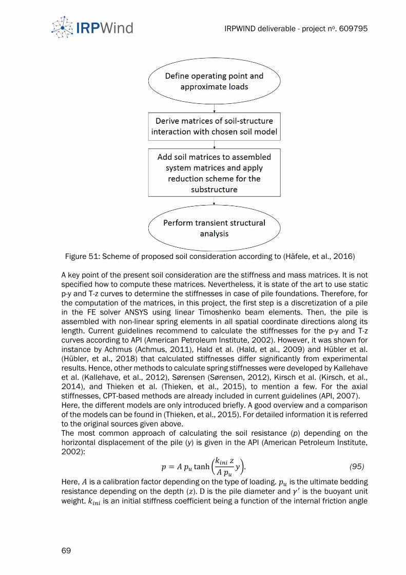
IRPWIND deliverable - project no. 609795
69
Figure 51: Scheme of proposed soil consideration according to (Häfele, et al., 2016)
A key point of the present soil consideration are the stiffness and mass matrices. It is not
specified how to compute these matrices. Nevertheless, it is state of the art to use static
p-y and T-z curves to determine the stiffnesses in case of pile foundations. Therefore, for
the computation of the matrices, in this project, the first step is a discretization of a pile
in the FE solver ANSYS using linear Timoshenko beam elements. Then, the pile is
assembled with non-linear spring elements in all spatial coordinate directions along its
length. Current guidelines recommend to calculate the stiffnesses for the p-y and T-z
curves according to API (American Petroleum Institute, 2002). However, it was shown for
instance by Achmus (Achmus, 2011), Hald et al. (Hald, et al., 2009) and Hübler et al.
(Hübler, et al., 2018) that calculated stiffnesses differ significantly from experimental
results. Hence, other methods to calculate spring stiffnesses were developed by Kallehave
et al. (Kallehave, et al., 2012), Sørensen (Sørensen, 2012), Kirsch et al. (Kirsch, et al.,
2014), and Thieken et al. (Thieken, et al., 2015), to mention a few. For the axial
stiffnesses, CPT-based methods are already included in current guidelines (API, 2007).
Here, the different models are only introduced briefly. A good overview and a comparison
of the models can be found in (Thieken, et al., 2015). For detailed information it is referred
to the original sources given above.
The most common approach of calculating the soil resistance (p) depending on the
horizontal displacement of the pile (y) is given in the API (American Petroleum Institute,
2002):
𝑝 = 𝐴 𝑝𝑢 tanh (𝑘𝑖𝑛𝑖 𝑧
𝐴 𝑝𝑢𝑦). (95)
Here, 𝐴 is a calibration factor depending on the type of loading. 𝑝𝑢 is the ultimate bedding
resistance depending on the depth (𝑧). D is the pile diameter and 𝛾′ is the buoyant unit
weight. 𝑘𝑖𝑛𝑖 is an initial stiffness coefficient being a function of the internal friction angle
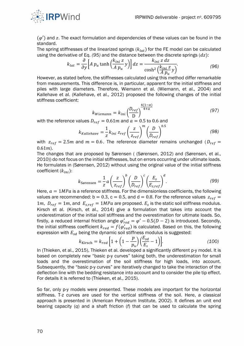
IRPWIND deliverable - project no. 609795
70
(𝜑′) and 𝑧. The exact formulation and dependencies of these values can be found in the
standard.
The spring stiffnesses of the linearized springs (𝑘𝑙𝑎𝑡) for the FE model can be calculated
using the derivative of Eq. (95) and the distance between the discrete springs (𝑑𝑧):
𝑘𝑙𝑎𝑡 =𝜕
𝜕𝑦[𝐴 𝑝𝑢 tanh (
𝑘𝑖𝑛𝑖 𝑧
𝐴 𝑝𝑢𝑦)] 𝑑𝑧 =
𝑘𝑖𝑛𝑖 𝑧 𝑑𝑧
cosh2 (𝑘𝑖𝑛𝑖 𝑧𝐴 𝑝𝑢
𝑦).
(96)
However, as stated before, the stiffnesses calculated using this method differ remarkable
from measurements. This difference is, in particular, apparent for the initial stiffness and
piles with large diameters. Therefore, Wiemann et al. (Wiemann, et al., 2004) and
Kallehave et al. (Kallehave, et al., 2012) proposed the following changes of the initial
stiffness coefficient:
𝑘𝑊𝑖𝑒𝑚𝑎𝑛𝑛 = 𝑘𝑖𝑛𝑖 (𝐷𝑟𝑒𝑓
D)
4(1−𝑎)4+𝑎
(97)
with the reference values 𝐷𝑟𝑒𝑓 = 0.61𝑚 and 𝑎 = 0.5 to 0.6 and
𝑘𝐾𝑎𝑙𝑙𝑒ℎ𝑎𝑣𝑒 =1
𝑧𝑘𝑖𝑛𝑖 𝑧𝑟𝑒𝑓 (
𝑧
𝑧𝑟𝑒𝑓)
𝑚
(𝐷
𝐷𝑟𝑒𝑓)
0.5
(98)
with 𝑧𝑟𝑒𝑓 = 2.5𝑚 and 𝑚 = 0.6 . The reference diameter remains unchanged (𝐷𝑟𝑒𝑓 =
0.61𝑚).
The changes that are proposed by Sørensen ( (Sørensen, 2012) and (Sørensen, et al.,
2010)) do not focus on the initial stiffnesses, but on errors occurring under ultimate loads.
He formulates in (Sørensen, 2012) without using the original value of the initial stiffness
coefficient (𝑘𝑖𝑛𝑖):
𝑘Sørensen =1
𝑧𝑎 (
𝑧
𝑧𝑟𝑒𝑓)
𝑏
(𝐷
𝐷𝑟𝑒𝑓)
𝑐
(𝐸𝑠𝐸𝑠,𝑟𝑒𝑓
)
𝑑
. (99)
Here, 𝑎 = 1𝑀𝑃𝑎 is a reference stiffness. For the dimensionless coefficients, the following
values are recommended: b = 0.3, c = 0.5, and d = 0.8. For the reference values 𝑧𝑟𝑒𝑓 =
1𝑚, 𝐷𝑟𝑒𝑓 = 1𝑚, and 𝐸𝑠,𝑟𝑒𝑓 = 1𝑀𝑃𝑎 are proposed. 𝐸𝑠 is the static soil stiffness modulus.
Kirsch et al. (Kirsch, et al., 2014) give a formulation that takes into account the
underestimation of the initial soil stiffness and the overestimation for ultimate loads. So,
firstly, a reduced internal friction angle 𝜑𝑟𝑒𝑑′ = 𝜑′ − 0.5(𝐷 − 2) is introduced. Secondly,
the initial stiffness coefficient 𝑘𝑟𝑒𝑑 = 𝑓(𝜑𝑟𝑒𝑑′ ) is calculated. Based on this, the following
expression with 𝐸𝑠𝑑 being the dynamic soil stiffness modulus is suggested:
𝑘Kirsch = 𝑘𝑟𝑒𝑑 [1 + (1 −𝑝
𝑝𝑢) (𝐸𝑠𝑑𝐸𝑠
− 1)]. (100)
In (Thieken, et al., 2015), Thieken et al. developed a significantly different p-y model. It is
based on completely new “basic p-y curves” taking both, the underestimation for small
loads and the overestimation of the soil stiffness for high loads, into account.
Subsequently, the “basic p-y curves” are iteratively changed to take the interaction of the
deflection line with the bedding resistance into account and to consider the pile tip effect.
For details it is referred to (Thieken, et al., 2015).
So far, only p-y models were presented. These models are important for the horizontal
stiffness. T-z curves are used for the vertical stiffness of the soil. Here, a classical
approach is presented in (American Petroleum Institute, 2002). It defines an unit end
bearing capacity (q) and a shaft friction (f) that can be used to calculate the spring

IRPWIND deliverable - project no. 609795
71
stiffnesses for the spring at the end of the pile (𝑘𝑞) and for springs parallel to the whole
pile ( 𝑘𝑎𝑥) , respectively. Both spring stiffnesses depend on the mobilized axial
displacement. In (American Petroleum Institute, 2002) the following recommendations
are given:
𝑞 = min (𝑞𝑚𝑎𝑥 , 𝑝′𝑁𝑞) (101)
and
𝑓 = min (𝑓𝑚𝑎𝑥, 𝐾 𝑝0tan (𝛿)). (102)
Here, 𝑞𝑚𝑎𝑥 is the limit unit end bearing capacity given in the standard for different soil
densities. The same applies for the limit skin friction (𝑓𝑚𝑎𝑥), the dimensionless bearing
capacity factor (𝑁𝑞) , and the soil pile friction angle (𝛿). 𝑝′ is the effective overburden
pressure at a given depth and 𝐾 is the coefficient of lateral pressure. This approach is
slightly changed in newer standards (API, 2007) and other methods of calculating the
shaft friction and the unit end bearing capacity are introduced. These methods (ICP, UWA,
FURGO and NGI) are mainly based on cone penetration tests (CPTs). For the unit skin
friction, the general equation (103) is proposed. Values for the constants a to e, u and 𝜈
are given in the standard for diffent approaches.
𝑓 = 𝑢 𝑞𝑐,𝑧 (𝜎𝑣0′
𝑝𝑎)
𝑎
𝐴𝑟𝑏 [max (𝜈,
𝐿 − 𝑧
𝐷)]−𝑐
(tan(𝛿𝑐𝑣)) 𝑑 [min (1,
𝐿 − 𝑧
𝐷
1
𝜈)]𝑒
. (103)
𝑞𝑐,𝑧 is the CPT cone tip resistance at depth 𝑧. 𝜎𝑣0′ is the soil effective vertical in-situ stress
at depth 𝑧. The atmospheric pressure is 𝑝𝑎. 𝐴𝑟 is defined as the pile displacement ratio
𝐴𝑟 = 1 − (𝐷𝑖
𝐷𝑜)2
using the inner and outer pile diameter (𝐷𝑖 and 𝐷𝑜). The embedded length
is 𝐿 and 𝛿𝑐𝑣 is the pile-soil constant volume interface friction angle.
For the unit end bearing capacity, different approaches, all based on the average value of
𝑞𝑐,𝑧 between 1.5 𝐷𝑜 above the pile tip to 1.5 𝐷𝑜 below pile tip level (𝑞𝑐𝑎𝑣15𝐷), are given in
the standard. The concept of FURGO-05 is given as an example. Details can be found in
(API, 2007).
𝑞𝐹𝑈𝑅𝐺𝑂 = 8.5 𝑝𝑎 (𝑞𝑐,𝑎𝑣,1.5𝐷 𝑝𝑎
)0.5
𝐴𝑟0.25. (104)
Summarizing the soil models: Many different soil models based on p-y and T-z curves exist
for the lateral and the axial stiffnesses of the soil. All these models can be used to
calculate the needed spring stiffnesses for the FE-model of the pile. For a chosen
operating point, the FE model can be linearized, and subsequently, it can be reduced to a
single mass and stiffness matrix using a Guyan reduction (Guyan, 2065). The computed
matrices have the following symmetric form, as axial and lateral behavior are uncoupled
and dissipation is neglected:
𝑲𝑠𝑜𝑖𝑙,𝑝𝑖𝑙𝑒 =
(
𝑘𝑥𝑥 0 0 0 −𝑘𝑥𝜃 00 𝑘𝑦𝑦 0 𝑘𝑦𝜙 0 0
0 0 𝑘𝑧𝑧 0 0 00 𝑘𝑦𝜙 0 𝑘𝜙𝜙 0 0
−𝑘𝑥𝜃 0 0 0 𝑘𝜃𝜃 00 0 0 0 0 𝑘𝜓𝜓)
. (105)
These stiffness and mass matrices can be used in the reduction scheme of FAST to
include soil characteristics in transient simulations as proposed.
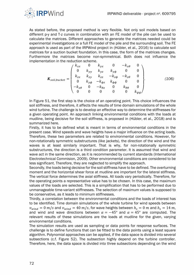
IRPWIND deliverable - project no. 609795
72
As stated before, the proposed method is very flexible. Not only soil models based on
different p-y and T-z curves in combination with an FE model of the pile can be used to
calculate the matrices. Different approaches to generate the matrices needed could be
experimental investigations or a full FE model of the pile and the surrounding soil. The FE
approach is used as part of the IRPWind project in (Hübler, et al., 2016) to calculate soil
matrices for a suction bucket foundation. In this case, the form of the matrices changes.
Furthermore the matrices become non-symmetrical. Both does not influence the
implementation in the reduction scheme.
𝑲𝑠𝑜𝑖𝑙,𝑏𝑢𝑐𝑘𝑒𝑡 =
(
𝑘𝑥𝑥 0 𝑘𝑦𝑥 0 −𝑘𝑥𝜃 0
0 𝑘𝑦𝑦 𝑘𝑦𝑧 𝑘𝑦𝜙 0 0
𝑘𝑧𝑥 𝑘𝑧𝑦 𝑘𝑧𝑧 −𝑘𝑧𝜙 −𝑘𝑧𝜃 0
0 𝑘𝑦𝜙 −𝑘𝜙𝑧 𝑘𝜙𝜙 0 0
−𝑘𝑥𝜃 0 −𝑘𝜃𝑧 0 𝑘𝜃𝜃 00 0 0 0 0 𝑘𝜓𝜓)
. (106)
In Figure 51, the first step is the choice of an operating point. This choice influences the
soil stiffness, and therefore, it affects the results of time domain simulations of the whole
wind turbine. The challenge is to develop an effective way to determine the stiffnesses for
a given operating point. An approach linking environmental conditions with the loads at
mudline, being decisive for the soil stiffness, is proposed in (Hübler, et al., 2018) and is
summarized here.
Firstly, it has to be defined what is meant in terms of environmental conditions in the
present case. Wind speeds and wave heights have a major influence on the acting loads.
Therefore, these two parameters are related to environmental conditions. However, for
non-rotationally symmetric substructures (like jackets), the direction of the wind and the
waves is at least similarly important. That is why, for non-rotationally symmetric
substructures, the direction is a third condition parameter. It is assumed that wind and
wave act in the same direction, as it is recommended by current standards (International
Electrotechnical Commision, 2009). Other environmental conditions are considered to be
less significant. Therefore, they are neglected to simplify the approach.
Secondly, the loads being decisive for the soil stiffness have to be defined. The overturning
moment and the horizontal shear force at mudline are important for the lateral stiffness.
The vertical force determines the axial stiffness. All loads vary periodically. Therefore, for
the operating points a representative value has to be chosen. In this case, the maximum
values of the loads are selected. This is a simplification that has to be performed due to
unmanageable time-variant stiffnesses. The selection of maximum values is supposed to
be conservative, as it leads to minimum stiffnesses.
Thirdly, a correlation between the environmental conditions and the loads of interest has
to be identified. Time domain simulations of the whole turbine for wind speeds between
𝑣𝑤𝑖𝑛𝑑 = 0 𝑚/𝑠 and 𝑣𝑤𝑖𝑛𝑑 = 40 𝑚/𝑠, for wave heights between ℎ𝑠 = 0 𝑚 and ℎ𝑠 = 14 𝑚,
and wind and wave directions between 𝛼 = −45° and 𝛼 = 45° are computed. The
relevant results of these simulations are the loads at mudline for the given, varying
environmental conditions.
The simulation results are used as sampling or data points for response surfaces. The
challenge is to define functions that can be fitted to the data points using a least square
algorithm. Polynomial approaches can be applied, if the data space is divided into several
subsections (c.f. Figure 52). The subsection highly depend on the turbine controller.
Therefore, here, the data space is divided into three subsections depending on the wind
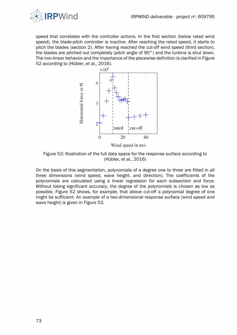
IRPWIND deliverable - project no. 609795
73
speed that correlates with the controller actions. In the first section (below rated wind
speed), the blade-pitch controller is inactive. After reaching the rated speed, it starts to
pitch the blades (section 2). After having reached the cut-off wind speed (third section),
the blades are pitched out completely (pitch angle of 90°) and the turbine is shut down.
The non-linear behavior and the importance of the piecewise definition is clarified in Figure
52 according to (Hübler, et al., 2016).
Figure 52: Illustration of the full data space for the response surface according to
(Hübler, et al., 2016)
On the basis of this segmentation, polynomials of a degree one to three are fitted in all
three dimensions (wind speed, wave height, and direction). The coefficients of the
polynomials are calculated using a linear regression for each subsection and force.
Without losing significant accuracy, the degree of the polynomials is chosen as low as
possible. Figure 52 shows, for example, that above cut-off a polynomial degree of one
might be sufficient. An example of a two-dimensional response surface (wind speed and
wave height) is given in Figure 53.
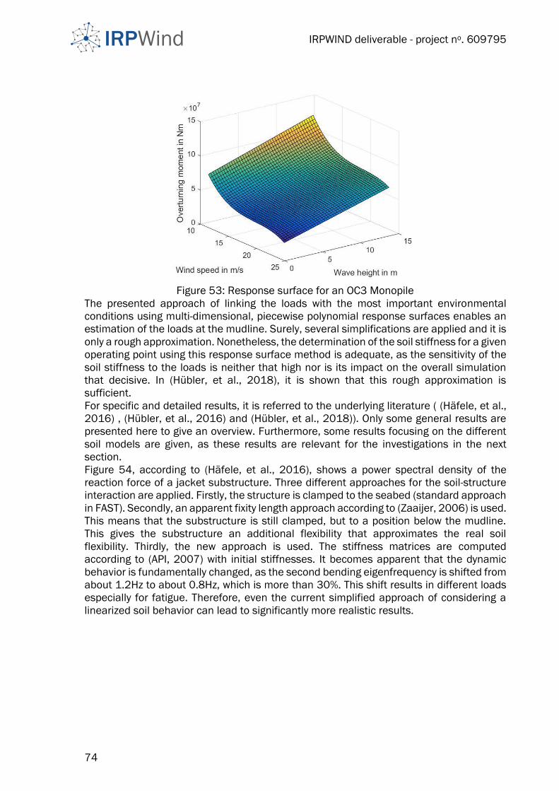
IRPWIND deliverable - project no. 609795
74
Figure 53: Response surface for an OC3 Monopile
The presented approach of linking the loads with the most important environmental
conditions using multi-dimensional, piecewise polynomial response surfaces enables an
estimation of the loads at the mudline. Surely, several simplifications are applied and it is
only a rough approximation. Nonetheless, the determination of the soil stiffness for a given
operating point using this response surface method is adequate, as the sensitivity of the
soil stiffness to the loads is neither that high nor is its impact on the overall simulation
that decisive. In (Hübler, et al., 2018), it is shown that this rough approximation is
sufficient.
For specific and detailed results, it is referred to the underlying literature ( (Häfele, et al.,
2016) , (Hübler, et al., 2016) and (Hübler, et al., 2018)). Only some general results are
presented here to give an overview. Furthermore, some results focusing on the different
soil models are given, as these results are relevant for the investigations in the next
section.
Figure 54, according to (Häfele, et al., 2016), shows a power spectral density of the
reaction force of a jacket substructure. Three different approaches for the soil-structure
interaction are applied. Firstly, the structure is clamped to the seabed (standard approach
in FAST). Secondly, an apparent fixity length approach according to (Zaaijer, 2006) is used.
This means that the substructure is still clamped, but to a position below the mudline.
This gives the substructure an additional flexibility that approximates the real soil
flexibility. Thirdly, the new approach is used. The stiffness matrices are computed
according to (API, 2007) with initial stiffnesses. It becomes apparent that the dynamic
behavior is fundamentally changed, as the second bending eigenfrequency is shifted from
about 1.2Hz to about 0.8Hz, which is more than 30%. This shift results in different loads
especially for fatigue. Therefore, even the current simplified approach of considering a
linearized soil behavior can lead to significantly more realistic results.
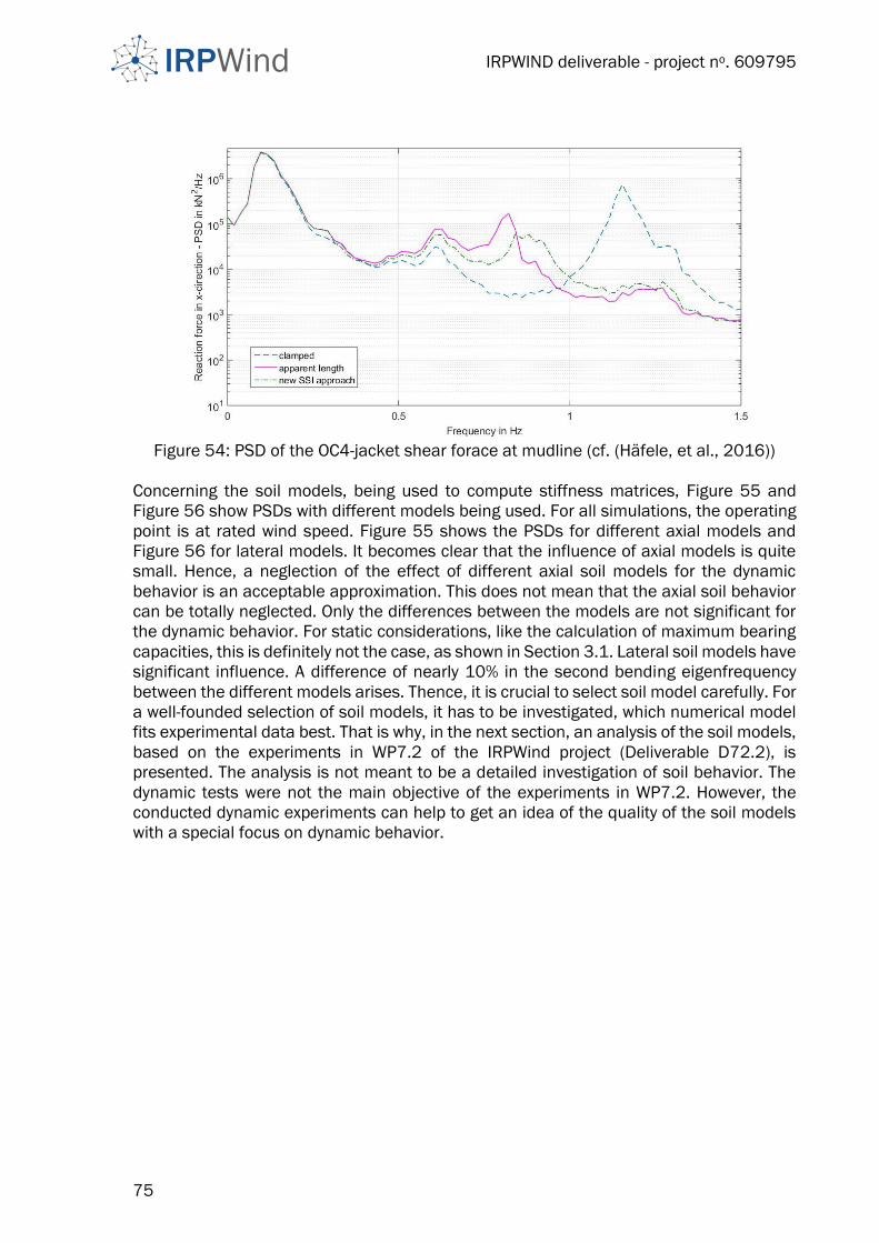
IRPWIND deliverable - project no. 609795
75
Figure 54: PSD of the OC4-jacket shear forace at mudline (cf. (Häfele, et al., 2016))
Concerning the soil models, being used to compute stiffness matrices, Figure 55 and
Figure 56 show PSDs with different models being used. For all simulations, the operating
point is at rated wind speed. Figure 55 shows the PSDs for different axial models and
Figure 56 for lateral models. It becomes clear that the influence of axial models is quite
small. Hence, a neglection of the effect of different axial soil models for the dynamic
behavior is an acceptable approximation. This does not mean that the axial soil behavior
can be totally neglected. Only the differences between the models are not significant for
the dynamic behavior. For static considerations, like the calculation of maximum bearing
capacities, this is definitely not the case, as shown in Section 3.1. Lateral soil models have
significant influence. A difference of nearly 10% in the second bending eigenfrequency
between the different models arises. Thence, it is crucial to select soil model carefully. For
a well-founded selection of soil models, it has to be investigated, which numerical model
fits experimental data best. That is why, in the next section, an analysis of the soil models,
based on the experiments in WP7.2 of the IRPWind project (Deliverable D72.2), is
presented. The analysis is not meant to be a detailed investigation of soil behavior. The
dynamic tests were not the main objective of the experiments in WP7.2. However, the
conducted dynamic experiments can help to get an idea of the quality of the soil models
with a special focus on dynamic behavior.
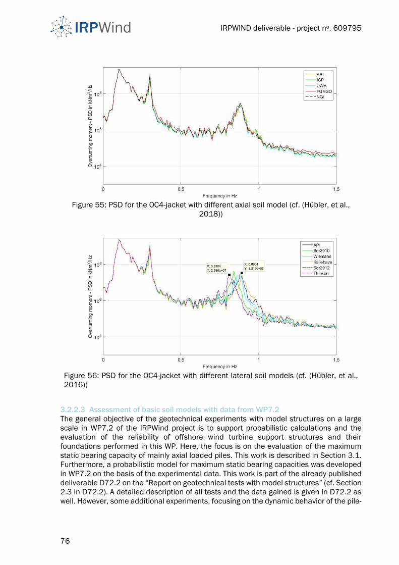
IRPWIND deliverable - project no. 609795
76
Figure 55: PSD for the OC4-jacket with different axial soil model (cf. (Hübler, et al.,
2018))
Figure 56: PSD for the OC4-jacket with different lateral soil models (cf. (Hübler, et al.,
2016))
3.2.2.3 Assessment of basic soil models with data from WP7.2
The general objective of the geotechnical experiments with model structures on a large
scale in WP7.2 of the IRPWind project is to support probabilistic calculations and the
evaluation of the reliability of offshore wind turbine support structures and their
foundations performed in this WP. Here, the focus is on the evaluation of the maximum
static bearing capacity of mainly axial loaded piles. This work is described in Section 3.1.
Furthermore, a probabilistic model for maximum static bearing capacities was developed
in WP7.2 on the basis of the experimental data. This work is part of the already published
deliverable D72.2 on the “Report on geotechnical tests with model structures” (cf. Section
2.3 in D72.2). A detailed description of all tests and the data gained is given in D72.2 as
well. However, some additional experiments, focusing on the dynamic behavior of the pile-
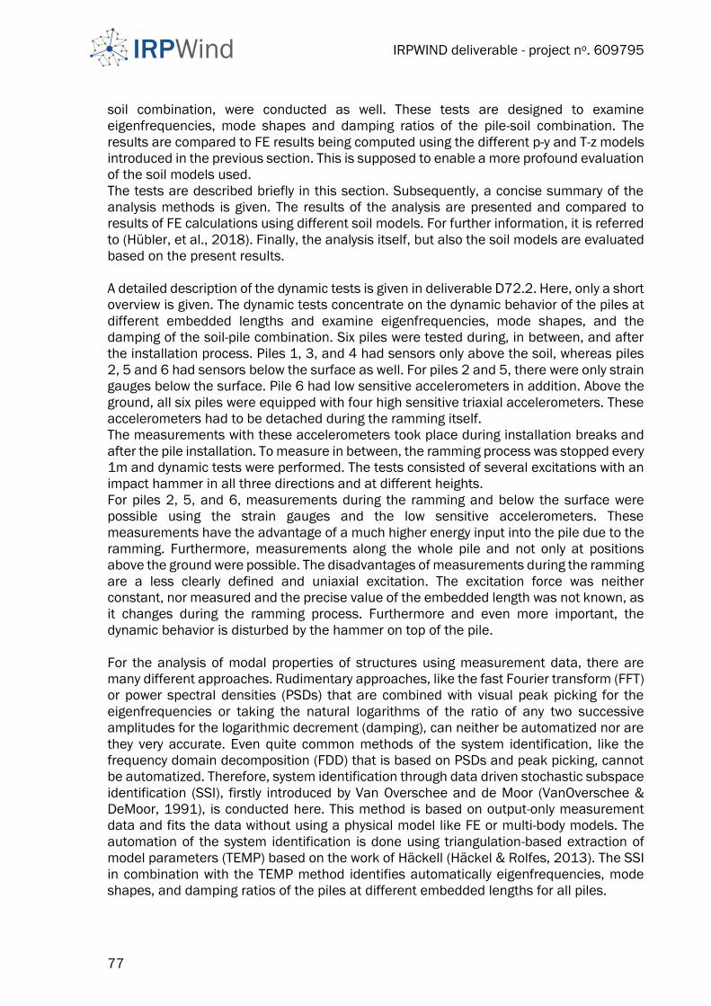
IRPWIND deliverable - project no. 609795
77
soil combination, were conducted as well. These tests are designed to examine
eigenfrequencies, mode shapes and damping ratios of the pile-soil combination. The
results are compared to FE results being computed using the different p-y and T-z models
introduced in the previous section. This is supposed to enable a more profound evaluation
of the soil models used.
The tests are described briefly in this section. Subsequently, a concise summary of the
analysis methods is given. The results of the analysis are presented and compared to
results of FE calculations using different soil models. For further information, it is referred
to (Hübler, et al., 2018). Finally, the analysis itself, but also the soil models are evaluated
based on the present results.
A detailed description of the dynamic tests is given in deliverable D72.2. Here, only a short
overview is given. The dynamic tests concentrate on the dynamic behavior of the piles at
different embedded lengths and examine eigenfrequencies, mode shapes, and the
damping of the soil-pile combination. Six piles were tested during, in between, and after
the installation process. Piles 1, 3, and 4 had sensors only above the soil, whereas piles
2, 5 and 6 had sensors below the surface as well. For piles 2 and 5, there were only strain
gauges below the surface. Pile 6 had low sensitive accelerometers in addition. Above the
ground, all six piles were equipped with four high sensitive triaxial accelerometers. These
accelerometers had to be detached during the ramming itself.
The measurements with these accelerometers took place during installation breaks and
after the pile installation. To measure in between, the ramming process was stopped every
1m and dynamic tests were performed. The tests consisted of several excitations with an
impact hammer in all three directions and at different heights.
For piles 2, 5, and 6, measurements during the ramming and below the surface were
possible using the strain gauges and the low sensitive accelerometers. These
measurements have the advantage of a much higher energy input into the pile due to the
ramming. Furthermore, measurements along the whole pile and not only at positions
above the ground were possible. The disadvantages of measurements during the ramming
are a less clearly defined and uniaxial excitation. The excitation force was neither
constant, nor measured and the precise value of the embedded length was not known, as
it changes during the ramming process. Furthermore and even more important, the
dynamic behavior is disturbed by the hammer on top of the pile.
For the analysis of modal properties of structures using measurement data, there are
many different approaches. Rudimentary approaches, like the fast Fourier transform (FFT)
or power spectral densities (PSDs) that are combined with visual peak picking for the
eigenfrequencies or taking the natural logarithms of the ratio of any two successive
amplitudes for the logarithmic decrement (damping), can neither be automatized nor are
they very accurate. Even quite common methods of the system identification, like the
frequency domain decomposition (FDD) that is based on PSDs and peak picking, cannot
be automatized. Therefore, system identification through data driven stochastic subspace
identification (SSI), firstly introduced by Van Overschee and de Moor (VanOverschee &
DeMoor, 1991), is conducted here. This method is based on output-only measurement
data and fits the data without using a physical model like FE or multi-body models. The
automation of the system identification is done using triangulation-based extraction of
model parameters (TEMP) based on the work of Häckell (Häckel & Rolfes, 2013). The SSI
in combination with the TEMP method identifies automatically eigenfrequencies, mode
shapes, and damping ratios of the piles at different embedded lengths for all piles.
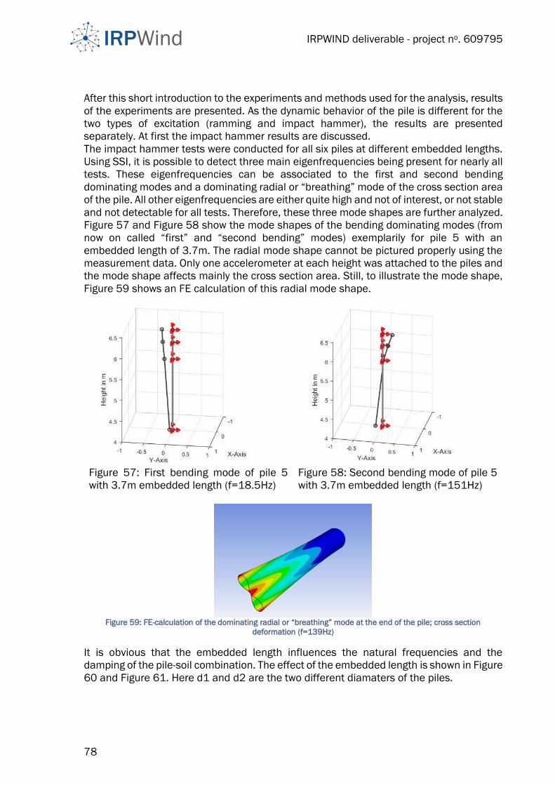
IRPWIND deliverable - project no. 609795
78
After this short introduction to the experiments and methods used for the analysis, results
of the experiments are presented. As the dynamic behavior of the pile is different for the
two types of excitation (ramming and impact hammer), the results are presented
separately. At first the impact hammer results are discussed.
The impact hammer tests were conducted for all six piles at different embedded lengths.
Using SSI, it is possible to detect three main eigenfrequencies being present for nearly all
tests. These eigenfrequencies can be associated to the first and second bending
dominating modes and a dominating radial or “breathing” mode of the cross section area
of the pile. All other eigenfrequencies are either quite high and not of interest, or not stable
and not detectable for all tests. Therefore, these three mode shapes are further analyzed.
Figure 57 and Figure 58 show the mode shapes of the bending dominating modes (from
now on called “first” and “second bending” modes) exemplarily for pile 5 with an
embedded length of 3.7m. The radial mode shape cannot be pictured properly using the
measurement data. Only one accelerometer at each height was attached to the piles and
the mode shape affects mainly the cross section area. Still, to illustrate the mode shape,
Figure 59 shows an FE calculation of this radial mode shape.
Figure 57: First bending mode of pile 5
with 3.7m embedded length (f=18.5Hz)
Figure 58: Second bending mode of pile 5
with 3.7m embedded length (f=151Hz)
Figure 59: FE-calculation of the dominating radial or “breathing” mode at the end of the pile; cross section
deformation (f=139Hz)
It is obvious that the embedded length influences the natural frequencies and the
damping of the pile-soil combination. The effect of the embedded length is shown in Figure
60 and Figure 61. Here d1 and d2 are the two different diamaters of the piles.
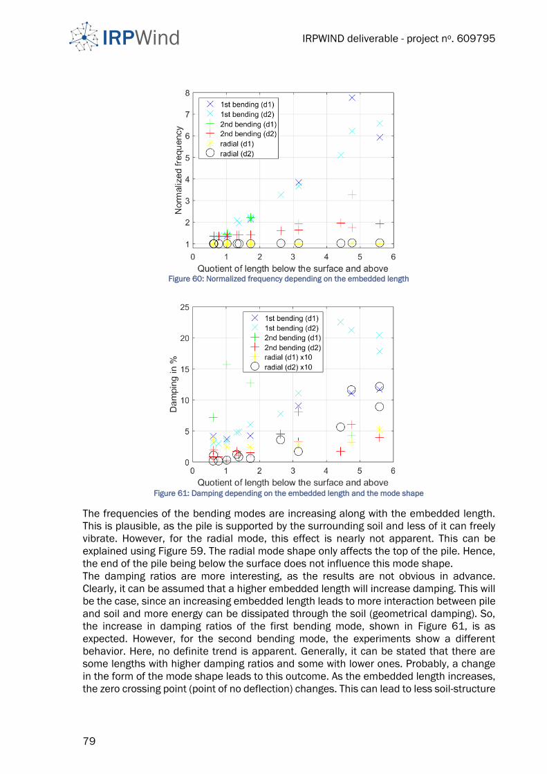
IRPWIND deliverable - project no. 609795
79
Figure 60: Normalized frequency depending on the embedded length
Figure 61: Damping depending on the embedded length and the mode shape
The frequencies of the bending modes are increasing along with the embedded length.
This is plausible, as the pile is supported by the surrounding soil and less of it can freely
vibrate. However, for the radial mode, this effect is nearly not apparent. This can be
explained using Figure 59. The radial mode shape only affects the top of the pile. Hence,
the end of the pile being below the surface does not influence this mode shape.
The damping ratios are more interesting, as the results are not obvious in advance.
Clearly, it can be assumed that a higher embedded length will increase damping. This will
be the case, since an increasing embedded length leads to more interaction between pile
and soil and more energy can be dissipated through the soil (geometrical damping). So,
the increase in damping ratios of the first bending mode, shown in Figure 61, is as
expected. However, for the second bending mode, the experiments show a different
behavior. Here, no definite trend is apparent. Generally, it can be stated that there are
some lengths with higher damping ratios and some with lower ones. Probably, a change
in the form of the mode shape leads to this outcome. As the embedded length increases,
the zero crossing point (point of no deflection) changes. This can lead to less soil-structure
IRPWIND deliverable - project no. 609795
80
interaction at higher embedded lengths, and therefore, to smaller damping ratios
(material damping in the soil). For the radial mode shape, firstly, it has to be pointed out
that the damping values are multiplied by a factor of ten in Figure 61. This is done for
reasons of clear illustration. Having that in mind, the damping for this mode shape is very
small. Again, this can be explained by the appearance of this mode shape in the
uppermost section of the pile. That is why there is nearly no interaction with the soil. Mainly
material damping of the pile itself occurs, which is much lower than geometrical or
material damping of the soil. Overall, the results of the damping have to be considered
with care. Damping data is, as it is quite common, scattering a lot. However, since fairly
high number of measurements was conducted, the results are still valid.
For the second part of the experiments, the dynamic behavior of the pile-soil combination
during the ramming process is analyzed. These experiments had the advantage of a much
higher energy input and of continuous measurements. On the downside, the excitation
was only in axial direction and the hammer on top of the pile is disturbing the dynamic
behavior of the pile. The data is analyzed using SSI and the TEMP method. Two mode
shapes are detected without doubt. This is again the radial mode and additionally the first
axial mode. The first bending mode is partly recognizable. Eigenfrequencies and damping
ratios over all hammer blows or embedded lengths are shown, exemplarily for pile 6, in
Figure 62 and Figure 63, respectively. Here, only the results of the strain gauges are
presented. The data of the 2000g accelerometers is comparable, but there are some
issues concerning the low sensitivities. For the eigenfrequencies, the high scattering
becomes apparent. Especially for the axial mode, there are high deviation. This is because
of low sensitivities in combination with high damping ratios and not totally free decay
processes (the hammer excitations are quite close to each other). Still, it can be
recognized that the frequency increases while the pile is driven into the soil. There are
some outliers at about 2.9m and 4m. It is assumed that these outliers are a result of the
ramming itself or of interaction effects of the hammer with the pile, since they disappear
after having stopped the ramming at 3m and 4.1m. It might be also possible that these
outliers are due to mode switches (i.e. another mode was detected). However, as there
are no other pronounced modes, this reason is fairly unlikely. The first bending mode can
only be detected in some cases. However, there is the same trend of higher frequencies
for higher embedded lengths. The results of the radial mode support the results achieved
by the impact hammer tests. There is nearly no change in the eigenfrequency over all
embedded lengths. For the damping ratios in Figure 63, firstly, it has to be explained why
there are such different, but stable results for different embedded lengths. Again, this can
be traced back to different ramming cycles. The ramming was stopped at 0.7m, 1.5m,
3m, 4.1m, 5m, 6m, and at the end at 6.7m. These values correspond quite well to the
different sections that can be seen in Figure 63 for the axial mode. Therefore, these
differences are not of predominating relevance for the pile behavior itself. They only
demonstrate how problematic the measurements during the ramming with hammer on
top of the pile are. More important are the high damping ratios and changes in the
damping. Firstly, the axial mode is heavily damped. This is the reason why it cannot be
detected by impact hammer tests. Secondly, all mode shapes experience nearly constant
damping ratios (or at least no trends are recognizable). This result does not agree with the
previous results and cannot be explained so far. Higher embedded lengths should result
in more soil-pile interaction, and therefore, in more damping. That is why this phenomena
has to be further investigated in following studies. An interaction effect with the hammer
on top of the pile has to be analyzed.

IRPWIND deliverable - project no. 609795
81
Figure 62: Normalized frequencies of pile 6 during the ramming process
Figure 63: Damping ratios of pile 6 during the ramming process
P-y and T-z based soil models are used in this report to calculate the needed soil matrices.
To conclude this section on soil models, the just presented results of the dynamic tests in
WP7.2 are compared to results of FE simulations. Here, the focus is on the dynamic
behavior. Only the experiments with impact hammer excitations are taken into account.
For the tests during the ramming, the precise embedded lengths are not known, and
therefore, comparisons would be less accurate. Furthermore, the load level during the
ramming is unknown. As the soil stiffness depends on the load level, numerical

IRPWIND deliverable - project no. 609795
82
calculations would only be rough estimates. For the FE calculations, the piles are modelled
as linear Timoshenko beam elements, and the surrounding soil is represented by springs
in all spatial coordinate directions along the embedded length of the pile. The spring
stiffnesses are based on the different soil models. The FE model is the same as in section
3.2.2.2 for the deviation of the soil matrices and as in (Hübler, et al., 2018). Computed
eigenfrequencies of the FE calculations are compared to the experimental results. This is
done for different embedded lengths. A consideration of damping ratios is not part of this
analysis, as the utilized soil models do not include damping. Furthermore, radial modes
are neglected, since beam elements are not capable of computing them. Excitations with
the impact hammer during the experiments do not lead to significant displacements of
the pile in the soil. Hence, it is only a marginal simplification if small loads, and therefore,
initial soil conditions are assumed.
To evaluate the different soil models, measured and calculated bending eigenfrequencies
are compared. Figure 64 and Figure 65 show the normalized first bending frequency of
the piles with the larger and smaller diameter for different embedded lengths respectively.
The frequencies are normalized with the experimental values. It becomes clear that the
results of the soil models significantly differ and mostly do not fit the experiments. The
standard model of the API predicts frequencies that are about 10% too low. The
approaches of Sørensen ( (Sørensen, et al., 2010), (Sørensen, 2012)) show even higher
deviations. This can be explained by the purpose of these approaches. They focus on
extreme loads, but in these experiments only small loads were applied. Wiemann et al.
(Wiemann, et al., 2004) concentrate on extreme loads as well. However, their approach
focuses on piles with large diameters and uses a reference diameter of 𝐷𝑟𝑒𝑓 = 0.61𝑚. As
the piles in the present experiments are of about the same diameter, the changes
compared to the API model are marginal. The model of Kallehave et al. (Kallehave, et al.,
2012) fits the experiments the best. For this approach, the focus is on initial conditions
as they are present here. However, in some cases, even this model shows differences of
about 25%. Thieken et al. (Thieken, et al., 2015) try to cover initial and ultimate conditions
with their new approach. However, it is clear that for initial conditions the eigenfrequencies
are massively overestimated. It has to be mentioned that the approach of Thieken et al.
is much more sensitive to varying loads. Therefore, for this approach, it might be a
significant simplification to assume initial conditions, as the hammer excitations still
introduce some loads, though these loads are fairly small. However, for loads greater than
zero the soil becomes significantly softer for this approach, and therefore, the calculated
eigenfrequencies – being to high so far - are getting closer to the measured ones. For all
other approaches, the effect of the non-zero loads, if present, is leading to greater
differences compared to the experimental results, as the preticted eigenfrequencies are
already to small. However, as neither the loads at mudline nor the displacements were
measured a quantitative assessment of this effect is not possible.
For the second bending mode, the identification is not that clear. Therefore, it is abstained
from judging the soil models on this basis as well. However, for the second bending mode,
the numerical calculations fit the experiments even worse, and the errors are changing
for different embedded lengths, which is not the case for the first bending mode. For the
sake of completeness, the normalized second bending eigenfrequencies for piles with
smaller diameters are displayed in Figure 66.
After all, the comparisons of experiments and numerical models show that none of these
soil models can really predict the dynamic behavior of the piles, as deviations of up to

IRPWIND deliverable - project no. 609795
83
25% for the best model occur. It has to be pointed out that all investigated p-y curves were
initially developed for static loads. Still, currently, they are used in dynamic wind turbine
applications. This fact explains, at least partly, the deviations between the numerical and
experimental results. However, if models are chosen carefully according to their intended
load conditions, model errors can be reduced. Models that focus on initial conditions can
deliver the best results for these conditions. Whether models that focus on ultimate loads
are best suitable for high load conditions or not, cannot be investigated using the present
data, but it would be valuable to investigate it.
Figure 64: Normalized first bending eigenfrequencies of the piles with larger diameter
for different embedded lengths calculated using different soil models
3.2.3 Statistical distributions of input parameters
Section 3.2.2 focuses on a time domain model of an offshore wind turbine including an
adequate soil model. This model can be used in deterministic and probabilistic
calculations. For deterministic calculations, only a single value for each input is needed,
whereas for probabilistic simulations, statistical distributions for all input parameters are
needed. In this section, statistical distributions for various inputs are derived. This is either
done from the literature or using real offshore measurement data. Since not all possible
parameters can be varied, the focus is on environmental conditions like wind, wave, and
soil conditions, material parameters of the substructure, and local geometrical
parameters of the substructure and foundation. Local geometrical parameters are, for
example, fabrication tolerances. Global or larger changes of the geometry, resulting from
designs changes, are not analyzed. All parameters being investigated are summarized in
Table 20. For soil properties, several values of the same parameter are applied, as the
soil model consists of three different layers. The same applies to substructure
components, as the substructure has various piles and braces with different wall
thicknesses etc.
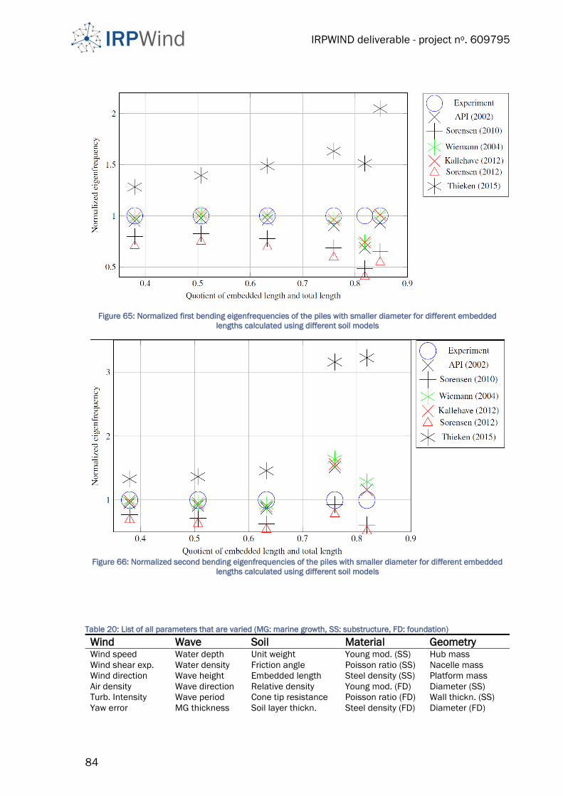
IRPWIND deliverable - project no. 609795
84
Figure 65: Normalized first bending eigenfrequencies of the piles with smaller diameter for different embedded
lengths calculated using different soil models
Figure 66: Normalized second bending eigenfrequencies of the piles with smaller diameter for different embedded
lengths calculated using different soil models
Table 20: List of all parameters that are varied (MG: marine growth, SS: substructure, FD: foundation)
Wind Wave Soil Material Geometry Wind speed Water depth Unit weight Young mod. (SS) Hub mass
Wind shear exp. Water density Friction angle Poisson ratio (SS) Nacelle mass
Wind direction Wave height Embedded length Steel density (SS) Platform mass
Air density Wave direction Relative density Young mod. (FD) Diameter (SS)
Turb. Intensity Wave period Cone tip resistance Poisson ratio (FD) Wall thickn. (SS)
Yaw error MG thickness Soil layer thickn. Steel density (FD) Diameter (FD)
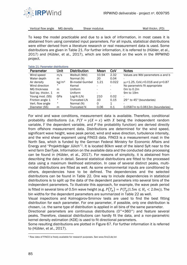
IRPWIND deliverable - project no. 609795
85
Vertical flow angle MG density Shear modulus Wall thickn. (FD)
To keep the model practicable and due to a lack of information, in most cases it is
abstained from using correlated input parameters. For all inputs, statistical distributions
were either derived from a literature research or real measurement data is used. Some
distributions are given in Table 21. For further information, it is referred to (Hübler, et al.,
2017) and (Hübler, et al., 2017), which are both based on the work in the IRPWIND
project.
Table 21: Parameter distributions
Parameter Unit Distribution Mean CoV Notes Wind speed m/s Weibull (Wbl) 10.94 2.32 Values are Wbl parameters a and b
Water depth m Normal (N) 20 0.04 -
Air density kg/m³ Bi-modal Gumbel 1.21 0.022 μ2=1.25, CoV2=0.016 and p=0.87
Wind direction ° Kernel - - No parametric fit appropriate
MG thickness m Uniform - - 0m to 0.2m
Soil lay. thickn. 1 m Uniform - - 9m to 19m
Young mod. (SS) GPa Log-N (LN) 210 0.02 -
Friction angle 1 ° Truncated LN 33 0.15 29° to 45°(boundaries)
Vert. flow angle ° Normal (N) 0 1 -
Diameter (SS) m Truncated N 0.06 0.1 0.0587m to 0.0613m (boundaries)
For wind and wave conditions, measurement data is available. Therefore, conditional
probability distributions (i.e. 𝑃(𝑌 = 𝑦|𝑋 = 𝑥) with 𝑋 being the independent random
variable, 𝑌 the dependent variable, and 𝑃 the probability function) are derived directly
from offshore measurement data. Distributions are determined for the wind speed,
significant wave height, wave peak period, wind and wave direction, turbulence intensity,
and the wind shear exponent using FINO3 data. FINO3 is a measurement mast in the
North Sea, which is funded by the German Federal Ministry for Economic Affairs and
Energy and “Projektträger Jülich”2. It is located 80km west of the island Sylt near to the
wind farm DanTysk. Information on the available data and the conducted data processing
can be found in (Hübler, et al., 2017). For reasons of simplicity, it is abstained from
describing the data in detail. Several statistical distributions are fitted to the processed
data using a maximum likelihood estimation. In case of several distinct peaks, multi-
modal distributions are fitted as well. As some environmental inputs are conditioned by
others, dependencies have to be defined. The dependencies and the selected
distributions can be found in Table 22. One way to include dependencies in statistical
distributions is to split up the data of the dependent parameters into several bins of the
independent parameters. To illustrate this approach, for example, the wave peak period
is fitted in several bins of 0.5m wave height (e.g. 𝑃(𝑇𝑝) = 𝑃(𝑇𝑝|1.5𝑚 ≤ 𝐻𝑠 < 2.0𝑚)). The
bin widths for the dependent parameters are summarized in Table 22 as well.
Visual inspections and Kolmogorov-Smirnov tests are used to find the best fitting
distribution for each parameter. For one parameter, if possible, only one distribution is
chosen, i.e. the same type of distribution is applied in all bins of the same parameter.
Directional parameters are continuous distributions (0°=360°) and feature several
peaks. Therefore, classical distributions can hardly fit the data, and a non-parametric
kernel density estimation (KDE) is used to fit directional parameters.
Some resulting distributions are plotted in Figure 67. For further information it is referred
to (Hübler, et al., 2017).
2 Raw data of FINO3 is freely available for research purposes. See www.fino3.de/en
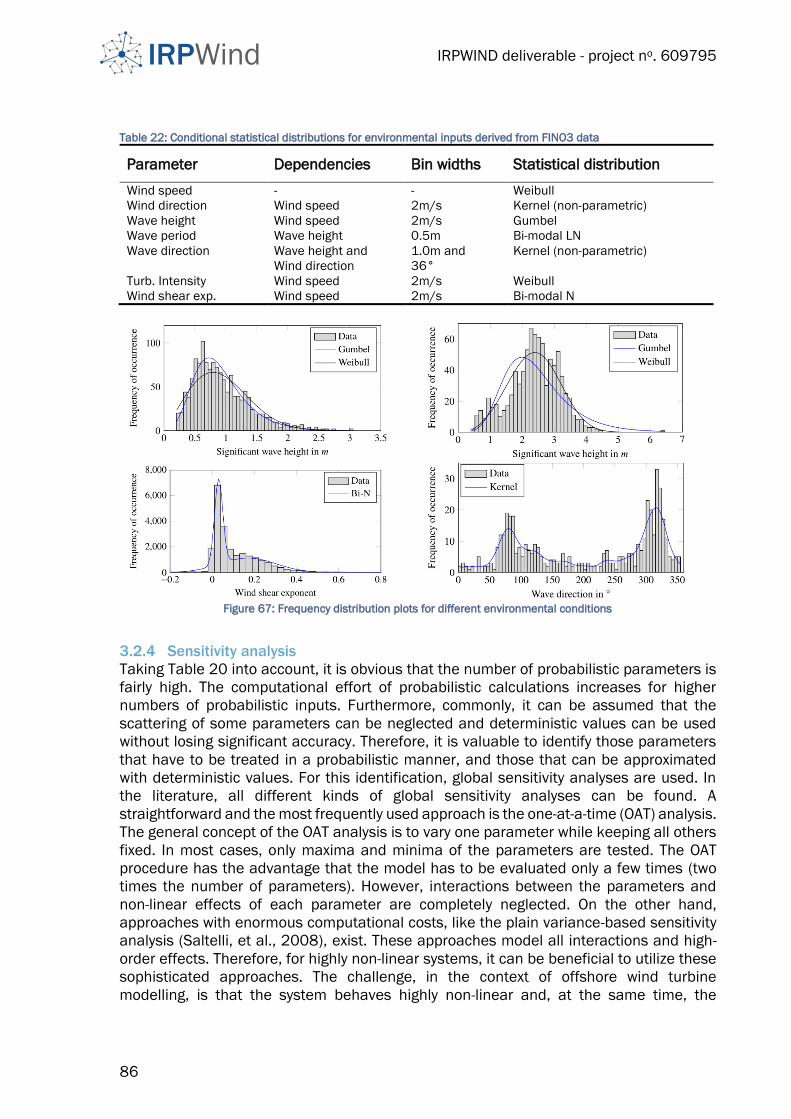
IRPWIND deliverable - project no. 609795
86
Table 22: Conditional statistical distributions for environmental inputs derived from FINO3 data
Parameter Dependencies Bin widths Statistical distribution
Wind speed - - Weibull
Wind direction Wind speed 2m/s Kernel (non-parametric)
Wave height Wind speed 2m/s Gumbel
Wave period Wave height 0.5m Bi-modal LN
Wave direction Wave height and
Wind direction
1.0m and
36°
Kernel (non-parametric)
Turb. Intensity Wind speed 2m/s Weibull
Wind shear exp. Wind speed 2m/s Bi-modal N
Figure 67: Frequency distribution plots for different environmental conditions
3.2.4 Sensitivity analysis
Taking Table 20 into account, it is obvious that the number of probabilistic parameters is
fairly high. The computational effort of probabilistic calculations increases for higher
numbers of probabilistic inputs. Furthermore, commonly, it can be assumed that the
scattering of some parameters can be neglected and deterministic values can be used
without losing significant accuracy. Therefore, it is valuable to identify those parameters
that have to be treated in a probabilistic manner, and those that can be approximated
with deterministic values. For this identification, global sensitivity analyses are used. In
the literature, all different kinds of global sensitivity analyses can be found. A
straightforward and the most frequently used approach is the one-at-a-time (OAT) analysis.
The general concept of the OAT analysis is to vary one parameter while keeping all others
fixed. In most cases, only maxima and minima of the parameters are tested. The OAT
procedure has the advantage that the model has to be evaluated only a few times (two
times the number of parameters). However, interactions between the parameters and
non-linear effects of each parameter are completely neglected. On the other hand,
approaches with enormous computational costs, like the plain variance-based sensitivity
analysis (Saltelli, et al., 2008), exist. These approaches model all interactions and high-
order effects. Therefore, for highly non-linear systems, it can be beneficial to utilize these
sophisticated approaches. The challenge, in the context of offshore wind turbine
modelling, is that the system behaves highly non-linear and, at the same time, the
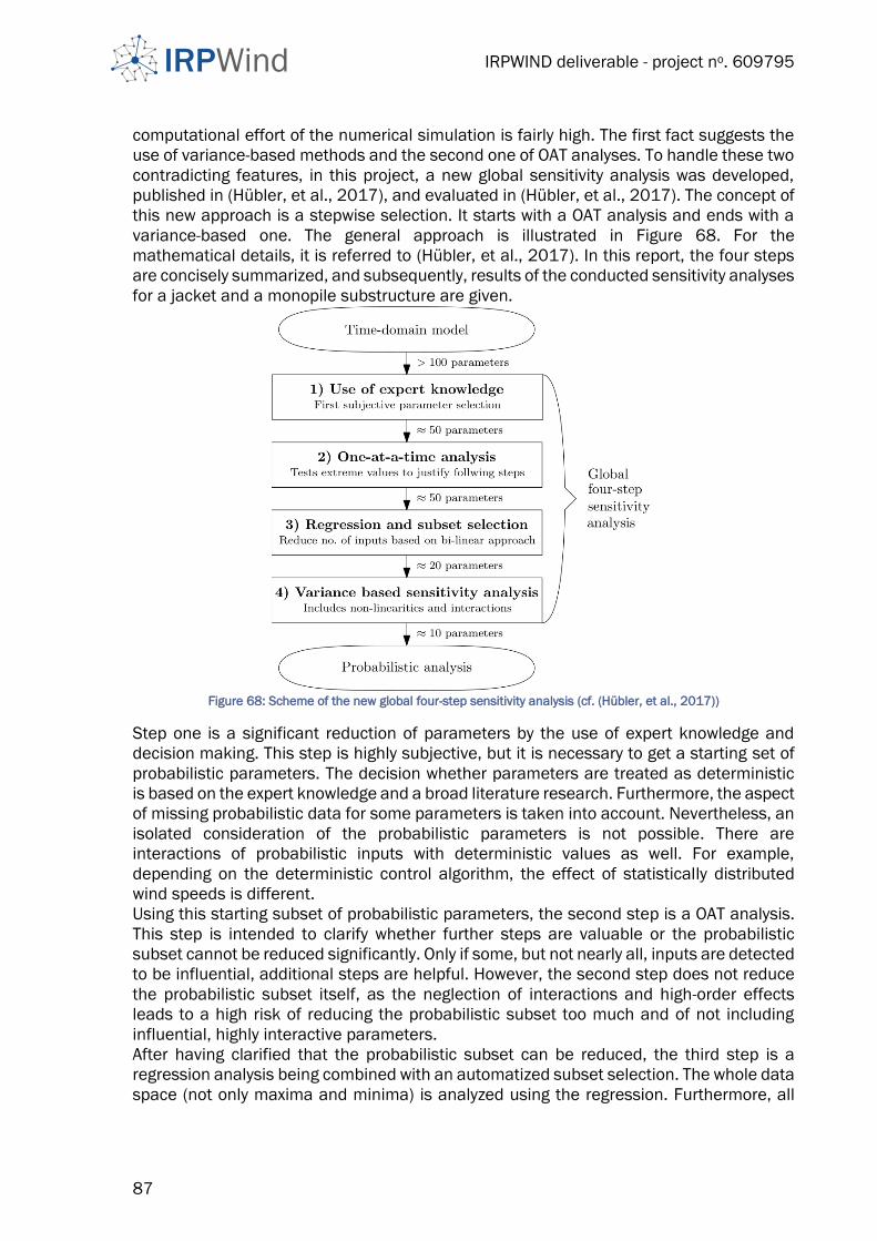
IRPWIND deliverable - project no. 609795
87
computational effort of the numerical simulation is fairly high. The first fact suggests the
use of variance-based methods and the second one of OAT analyses. To handle these two
contradicting features, in this project, a new global sensitivity analysis was developed,
published in (Hübler, et al., 2017), and evaluated in (Hübler, et al., 2017). The concept of
this new approach is a stepwise selection. It starts with a OAT analysis and ends with a
variance-based one. The general approach is illustrated in Figure 68. For the
mathematical details, it is referred to (Hübler, et al., 2017). In this report, the four steps
are concisely summarized, and subsequently, results of the conducted sensitivity analyses
for a jacket and a monopile substructure are given.
Figure 68: Scheme of the new global four-step sensitivity analysis (cf. (Hübler, et al., 2017))
Step one is a significant reduction of parameters by the use of expert knowledge and
decision making. This step is highly subjective, but it is necessary to get a starting set of
probabilistic parameters. The decision whether parameters are treated as deterministic
is based on the expert knowledge and a broad literature research. Furthermore, the aspect
of missing probabilistic data for some parameters is taken into account. Nevertheless, an
isolated consideration of the probabilistic parameters is not possible. There are
interactions of probabilistic inputs with deterministic values as well. For example,
depending on the deterministic control algorithm, the effect of statistically distributed
wind speeds is different.
Using this starting subset of probabilistic parameters, the second step is a OAT analysis.
This step is intended to clarify whether further steps are valuable or the probabilistic
subset cannot be reduced significantly. Only if some, but not nearly all, inputs are detected
to be influential, additional steps are helpful. However, the second step does not reduce
the probabilistic subset itself, as the neglection of interactions and high-order effects
leads to a high risk of reducing the probabilistic subset too much and of not including
influential, highly interactive parameters.
After having clarified that the probabilistic subset can be reduced, the third step is a
regression analysis being combined with an automatized subset selection. The whole data
space (not only maxima and minima) is analyzed using the regression. Furthermore, all

IRPWIND deliverable - project no. 609795
88
parameters are varied at the same time. However, regressions give only a (in this work bi-
linear) approximation of the real simulation model. Due to the bi-linear approximation,
high-order effects are neglected in this step, but some interaction effects are covered. A
better alternative for this third step compared to the bi-linear regression is presented in
(Hübler, et al., 2017). There, a kriging meta-model is proposed, and the better
performance is shown.
The fourth and last step of the multi-step sensitivity analysis is a global variance-based
sensitivity analysis. This analysis includes all non-linear high-order effects and interactions
between all input parameters. Therefore, on the one hand, it conserves the whole
complexity of the time domain model. On the other hand, it needs a large number of model
evaluations, as conditional variances are analyzed. This means, the influence of keeping
one factor fixed on the total variance is investigated. A variance-based analysis needs
𝑛 × (𝑚 + 2) model evaluations, with 𝑚 being the number of inputs and 𝑛 the number
samples (>750). This leads to more than 35,000 model evaluations for 50 parameters
compared to 100 model evaluations for the OAT analysis (2 × 𝑚). The use of the four-step
approach can reduce the number of model evaluation by a factor of about four compared
to the plain variance-based approach without neglecting non-linear effects.
The proposed four-step approach is used to identify the significant probabilistic
parameters of two substructures of offshore wind turbines (a jacket and a monopile
substructure) and for different outputs (ultimate and fatigue loads). For details in the
modelling and interim results, it is referred to (Hübler, et al., 2017). Here, only the overall
and general conclusions concerning non-influential and the most important parameters
are stated. For both substructures, only a very limited number of parameters is really
influential. Some parameter, like the internal friction angle or the unit weight of the soil
(for the monopile), influence all outputs, whereas others only influence either ultimate or
fatigue loads. Resonance effects are highly influenced by soil and geometrical
parameters. This can be concluded, as for soil and geometric parameters total effects are
much higher than first order indices. This means that they exhibit interaction effects. For
other parameters, like the air density, this is not the case. For these parameters,
interaction is less pronounced. Furthermore, interaction effects are more relevant for the
fatigue loads. After all, the parameters in Table 23 are the most influential ones for the
monopile and the jacket, respectively. These parameters are, as shown, structure
dependent. An additional slight site dependency is probable. Still, the most influential
parameters in any case are five environmental conditions determining the wind and wave
loads (wind speed and direction and wave height, period, and direction). At least these
five parameters should always be treated in a probabilistic manner. So far, in most cases,
only the two wind parameters are varied (by using several bins). The three wave inputs are
only changed deterministically depending on the wind speed and are constant in each
wind speed bin.
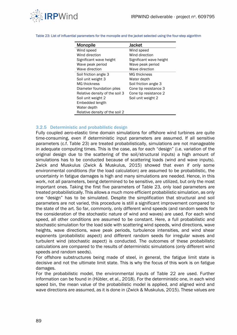
IRPWIND deliverable - project no. 609795
89
Table 23: List of influential parameters for the monopile and the jacket selected using the four-step algorithm
Monopile Jacket Wind speed Wind speed
Wind direction Wind direction
Significant wave height Significant wave height
Wave peak period Wave peak period
Wave direction Wave direction
Soil friction angle 3 MG thickness
Soil unit weight 3 Water depth
MG thickness Soil friction angle 3
Diameter foundation piles Cone tip resistance 3
Relative density of the soil 3 Cone tip resistance 2
Soil unit weight 2 Soil unit weight 2
Embedded length
Water depth
Relative density of the soil 2
3.2.5 Deterministic and probabilistic design
Fully coupled aero-elastic time domain simulations for offshore wind turbines are quite
time-consuming, even if deterministic input parameters are assumed. If all sensitive
parameters (c.f. Table 23) are treated probabilistically, simulations are not manageable
in adequate computing times. This is the case, as for each “design” (i.e. variation of the
original design due to the scattering of the soil/structural inputs) a high amount of
simulations has to be conducted because of scattering loads (wind and wave inputs).
Zwick and Muskulus (Zwick & Muskulus, 2015) showed that even if only some
environmental conditions (for the load calculation) are assumed to be probabilistic, the
uncertainty in fatigue damages is high and many simulations are needed. Hence, in this
work, not all parameters, being determined to be sensitive, are utilized, but only the most
important ones. Taking the first five parameters of Table 23, only load parameters are
treated probabilistically. This allows a much more efficient probabilistic simulation, as only
one “design” has to be simulated. Despite the simplification that structural and soil
parameters are not varied, this procedure is still a significant improvement compared to
the state of the art. So far, commonly, only different wind speeds (and random seeds for
the consideration of the stochastic nature of wind and waves) are used. For each wind
speed, all other conditions are assumed to be constant. Here, a full probabilistic and
stochastic simulation for the load side with scattering wind speeds, wind directions, wave
heights, wave directions, wave peak periods, turbulence intensities, and wind shear
exponents (probabilistic aspect) and different random seeds for irregular waves and
turbulent wind (stochastic aspect) is conducted. The outcomes of these probabilistic
calculations are compared to the results of deterministic simulations (only different wind
speeds and random seeds).
For offshore substructures being made of steel, in general, the fatigue limit state is
decisive and not the ultimate limit state. This is why the focus of this work is on fatigue
damages.
For the probabilistic model, the environmental inputs of Table 22 are used. Further
information can be found in (Hübler, et al., 2018). For the deterministic one, in each wind
speed bin, the mean value of the probabilistic model is applied, and aligned wind and
wave directions are assumed, as it is done in (Zwick & Muskulus, 2015). These values are
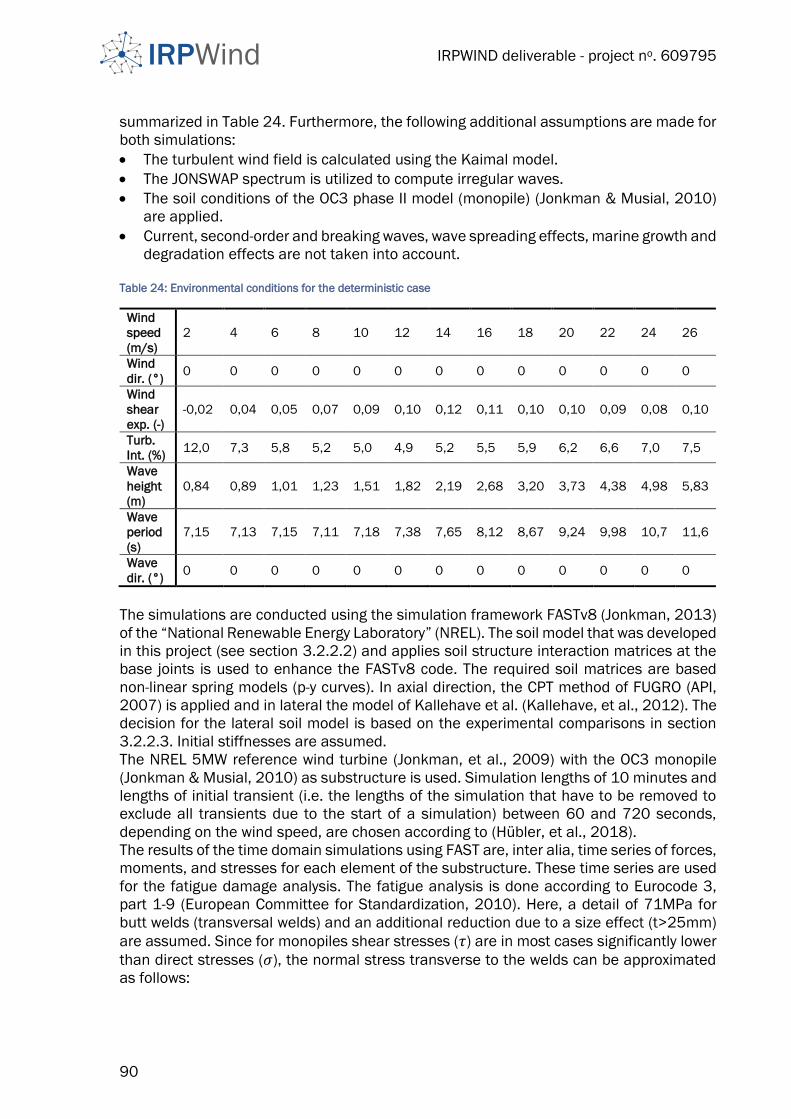
IRPWIND deliverable - project no. 609795
90
summarized in Table 24. Furthermore, the following additional assumptions are made for
both simulations:
• The turbulent wind field is calculated using the Kaimal model.
• The JONSWAP spectrum is utilized to compute irregular waves.
• The soil conditions of the OC3 phase II model (monopile) (Jonkman & Musial, 2010)
are applied.
• Current, second-order and breaking waves, wave spreading effects, marine growth and
degradation effects are not taken into account.
Table 24: Environmental conditions for the deterministic case
Wind
speed
(m/s)
2 4 6 8 10 12 14 16 18 20 22 24 26
Wind
dir. (°) 0 0 0 0 0 0 0 0 0 0 0 0 0
Wind
shear
exp. (-)
-0,02 0,04 0,05 0,07 0,09 0,10 0,12 0,11 0,10 0,10 0,09 0,08 0,10
Turb.
Int. (%) 12,0 7,3 5,8 5,2 5,0 4,9 5,2 5,5 5,9 6,2 6,6 7,0 7,5
Wave
height
(m)
0,84 0,89 1,01 1,23 1,51 1,82 2,19 2,68 3,20 3,73 4,38 4,98 5,83
Wave
period
(s)
7,15 7,13 7,15 7,11 7,18 7,38 7,65 8,12 8,67 9,24 9,98 10,7 11,6
Wave
dir. (°) 0 0 0 0 0 0 0 0 0 0 0 0 0
The simulations are conducted using the simulation framework FASTv8 (Jonkman, 2013)
of the “National Renewable Energy Laboratory” (NREL). The soil model that was developed
in this project (see section 3.2.2.2) and applies soil structure interaction matrices at the
base joints is used to enhance the FASTv8 code. The required soil matrices are based
non-linear spring models (p-y curves). In axial direction, the CPT method of FUGRO (API,
2007) is applied and in lateral the model of Kallehave et al. (Kallehave, et al., 2012). The
decision for the lateral soil model is based on the experimental comparisons in section
3.2.2.3. Initial stiffnesses are assumed.
The NREL 5MW reference wind turbine (Jonkman, et al., 2009) with the OC3 monopile
(Jonkman & Musial, 2010) as substructure is used. Simulation lengths of 10 minutes and
lengths of initial transient (i.e. the lengths of the simulation that have to be removed to
exclude all transients due to the start of a simulation) between 60 and 720 seconds,
depending on the wind speed, are chosen according to (Hübler, et al., 2018).
The results of the time domain simulations using FAST are, inter alia, time series of forces,
moments, and stresses for each element of the substructure. These time series are used
for the fatigue damage analysis. The fatigue analysis is done according to Eurocode 3,
part 1-9 (European Committee for Standardization, 2010). Here, a detail of 71MPa for
butt welds (transversal welds) and an additional reduction due to a size effect (t>25mm)
are assumed. Since for monopiles shear stresses (𝜏) are in most cases significantly lower
than direct stresses (𝜎), the normal stress transverse to the welds can be approximated
as follows:
IRPWIND deliverable - project no. 609795
91
𝜎⊥ =𝐹𝑧𝐴+√𝑀𝑥
2 +𝑀𝑦2
𝑆, (107)
where, 𝐴 and 𝑆 are the cross section area and the section modulus, respectively. This
approach is a conservative simplification, as the maximum normal stress ( 𝑀 =
√𝑀𝑥2 +𝑀𝑦
2) is assumed independent of the wind direction. For all hot spot stresses, a
Rainflow counting evaluates the stress cycles. A conservative linear damage accumulation
according to the Palmgren-Miner rule is assumed, as recommended by the current
standards. The damage (𝐷𝑗) for each time series (𝑗) is calculated using the number of
cycles (𝑛𝑘) associated to a stress amplitude (Δ𝜎⊥,𝑘) and the endurance (maximum number
of cycles; 𝑁𝑘 ) for the same stress amplitude. 𝐾 is the number of considered stress
amplitudes:
𝐷𝑗 =∑𝑛𝑘𝑁𝑘
𝐾
𝑘=1
, (108)
The slope of the S-N curve is three before and five after the fatigue limit. This differs slightly
from the Eurocode approach, where an additional cut-off limit at 𝑁 = 108 is presumed.
The damage at each position of the substructure is calculated by adding up the resulting
damages of all 10 minute time series, weighting them by their occurrence probability, and
extrapolating them to 20 years lifetime (cf. Equation (109)). The overall lifetime damage
of the substructure is determined by taking the maximum damage of all positions along
the substructure. A detailed description of the damage calculations procedure is given in
(Hübler, et al., 2018).
3.2.6 Damage distribution and failure probabilities
Due to the use of probabilistic input parameters the overall fatigue damage is scattering,
and therefore, it subjected to high uncertainties, if limited sampling is applied, which is
always the case due to limited computational resources. For a jacket substructure, Zwick
and Muskulus (Zwick & Muskulus, 2015) already showed that, even for deterministic
inputs (only different seeds and wind speeds) the error in fatigue damages due to finite
sampling occurring with a probability of 1% (1% error) is up to 29%, if six 10min
simulations are conducted. For probabilistic environmental states, scattering in each wind
speed bin, a considerable increase in the uncertainty of the lifetime damage due to finite
sampling is predicted. This increase is, for example, shown by Häfele et al. (Häfele, et al.,
2017) (Häfele, et al., 2017). Therefore, a study of convergence to determine the number
of simulations (𝑁) that is needed to determine the damage probability density function
(PDF) with a certain reliability is conducted. For this purpose, 10000 simulations for the
probabilistic case and 500 for the deterministic one are carried out in each wind speed
bin. Subsequently, 10000 random combinations of 𝑁𝑚𝑖𝑛 = 6 up to 𝑁𝑚𝑎𝑥 = 10000
simulations (𝑁𝑚𝑎𝑥 = 500 for the deterministic case) are selected using a bootstrapping
procedure. The bootstrapping approach allows to approximate the uncertainty for different
combination sizes. As the uncertainty depends on the wind speed, Figure 69 (right) shows
the 1% error for the probabilistic case for all wind speeds and several combinations sizes.
As a comparison, Figure 69 (left) displays the deterministic case. The highly differently
scaled vertical axes should be noted.
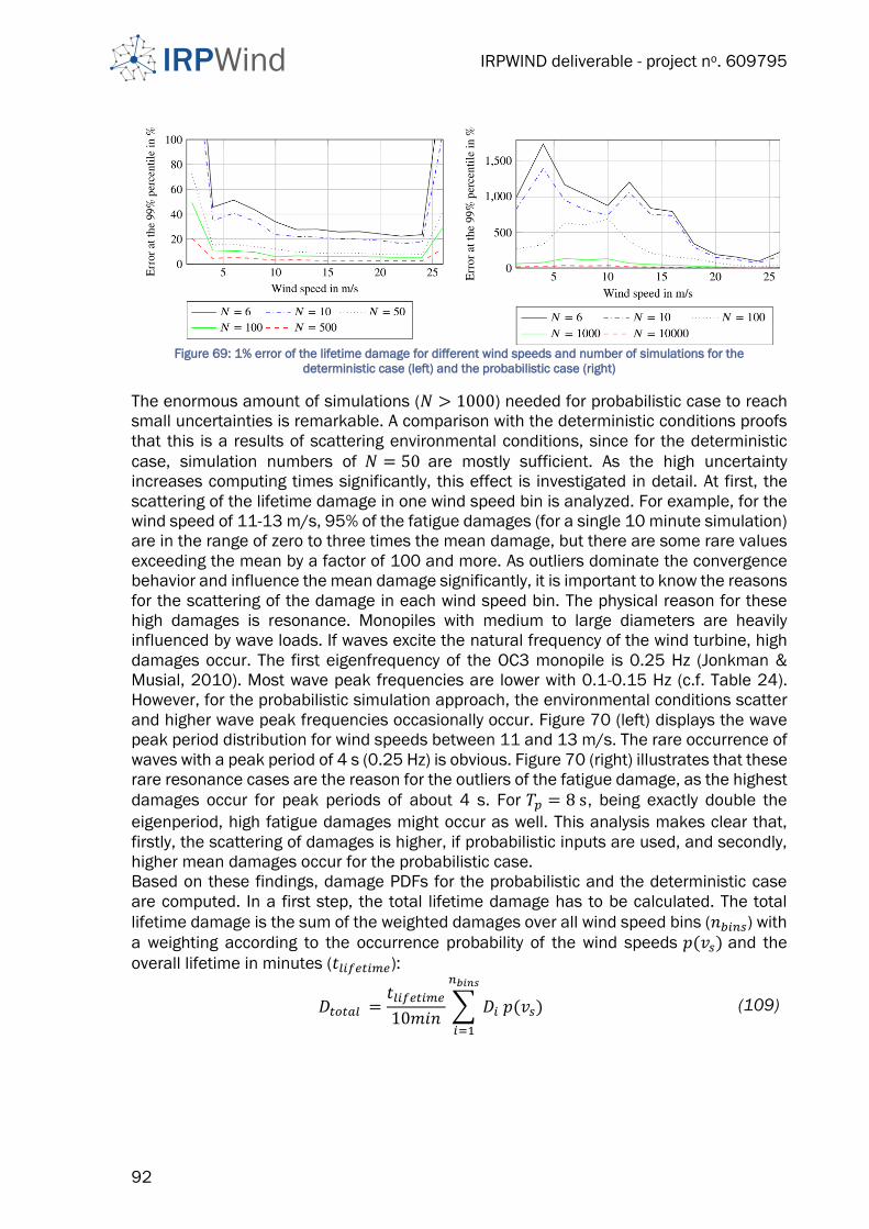
IRPWIND deliverable - project no. 609795
92
Figure 69: 1% error of the lifetime damage for different wind speeds and number of simulations for the
deterministic case (left) and the probabilistic case (right)
The enormous amount of simulations (𝑁 > 1000) needed for probabilistic case to reach
small uncertainties is remarkable. A comparison with the deterministic conditions proofs
that this is a results of scattering environmental conditions, since for the deterministic
case, simulation numbers of 𝑁 = 50 are mostly sufficient. As the high uncertainty
increases computing times significantly, this effect is investigated in detail. At first, the
scattering of the lifetime damage in one wind speed bin is analyzed. For example, for the
wind speed of 11-13 m/s, 95% of the fatigue damages (for a single 10 minute simulation)
are in the range of zero to three times the mean damage, but there are some rare values
exceeding the mean by a factor of 100 and more. As outliers dominate the convergence
behavior and influence the mean damage significantly, it is important to know the reasons
for the scattering of the damage in each wind speed bin. The physical reason for these
high damages is resonance. Monopiles with medium to large diameters are heavily
influenced by wave loads. If waves excite the natural frequency of the wind turbine, high
damages occur. The first eigenfrequency of the OC3 monopile is 0.25 Hz (Jonkman &
Musial, 2010). Most wave peak frequencies are lower with 0.1-0.15 Hz (c.f. Table 24).
However, for the probabilistic simulation approach, the environmental conditions scatter
and higher wave peak frequencies occasionally occur. Figure 70 (left) displays the wave
peak period distribution for wind speeds between 11 and 13 m/s. The rare occurrence of
waves with a peak period of 4 s (0.25 Hz) is obvious. Figure 70 (right) illustrates that these
rare resonance cases are the reason for the outliers of the fatigue damage, as the highest
damages occur for peak periods of about 4 s. For 𝑇𝑝 = 8 s, being exactly double the
eigenperiod, high fatigue damages might occur as well. This analysis makes clear that,
firstly, the scattering of damages is higher, if probabilistic inputs are used, and secondly,
higher mean damages occur for the probabilistic case.
Based on these findings, damage PDFs for the probabilistic and the deterministic case
are computed. In a first step, the total lifetime damage has to be calculated. The total
lifetime damage is the sum of the weighted damages over all wind speed bins (𝑛𝑏𝑖𝑛𝑠) with
a weighting according to the occurrence probability of the wind speeds 𝑝(𝑣𝑠) and the
overall lifetime in minutes (𝑡𝑙𝑖𝑓𝑒𝑡𝑖𝑚𝑒):
𝐷𝑡𝑜𝑡𝑎𝑙 =𝑡𝑙𝑖𝑓𝑒𝑡𝑖𝑚𝑒
10𝑚𝑖𝑛∑ 𝐷𝑖 𝑝(𝑣𝑠)
𝑛𝑏𝑖𝑛𝑠
𝑖=1
(109)
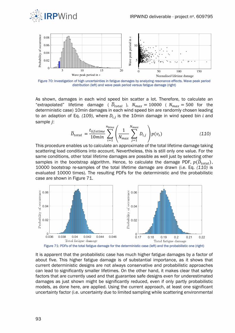
IRPWIND deliverable - project no. 609795
93
Figure 70: Investigation of high uncertainties in fatigue damages by analyzing resonance effects. Wave peak period
distribution (left) and wave peak period versus fatigue damage (right)
As shown, damages in each wind speed bin scatter a lot. Therefore, to calculate an
“extrapolated” lifetime damage ( 𝑡𝑜𝑡𝑎𝑙 ), 𝑁𝑚𝑎𝑥 = 10000 ( 𝑁𝑚𝑎𝑥 = 500 for the
deterministic case) 10min damages in each wind speed bin are randomly chosen leading
to an adaption of Eq. (109), where 𝐷𝑖,𝑗 is the 10min damage in wind speed bin 𝑖 and
sample 𝑗:
𝑡𝑜𝑡𝑎𝑙 =𝑡𝑙𝑖𝑓𝑒𝑡𝑖𝑚𝑒
10𝑚𝑖𝑛∑ (
1
𝑁𝑚𝑎𝑥∑ 𝐷𝑖,𝑗
𝑁𝑚𝑎𝑥
𝑗=1
)𝑝(𝑣𝑠)
𝑛𝑏𝑖𝑛𝑠
𝑖=1
(110)
This procedure enables us to calculate an approximate of the total lifetime damage taking
scattering load conditions into account. Nevertheless, this is still only one value. For the
same conditions, other total lifetime damages are possible as well just by selecting other
samples in the bootstrap algorithm. Hence, to calculate the damage PDF, 𝑝(𝑡𝑜𝑡𝑎𝑙) ,
10000 bootstrap re-samples of the total lifetime damage are drawn (i.e. Eq. (110) is
evaluated 10000 times). The resulting PDFs for the deterministic and the probabilistic
case are shown in Figure 71.
Figure 71: PDFs of the total fatigue damage for the deterministic case (left) and the probabilistic one (right)
It is apparent that the probabilistic case has much higher fatigue damages by a factor of
about five. This higher fatigue damage is of substantial importance, as it shows that
current deterministic designs are not always conservative and probabilistic approaches
can lead to significantly smaller lifetimes. On the other hand, it makes clear that safety
factors that are currently used and that guarantee safe designs even for underestimated
damages as just shown might be significantly reduced, even if only partly probabilistic
models, as done here, are applied. Using the current approach, at least one significant
uncertainty factor (i.e. uncertainty due to limited sampling while scattering environmental
IRPWIND deliverable - project no. 609795
94
conditions are applied) is identified. It has to be mentioned that the computational effort
of probabilistic approach is significantly higher. Here, twenty times more simulations were
used.
3.2.7 Summary and conclusion
The general aim of the work, described in section 3.2, is to conduct probabilistic
calculations of fully coupled offshore wind turbines to gain a first insight in the reliability
of substructures, based on sophisticated, non-linear aero-elastic simulations.
Furthermore, the objective was to create a basis for SF calibration, and to compare the
results of deterministic simulations and probabilistic ones.
Although it has to be mentioned that several simplifications are applied, the general aim
was achieved, and a comparison between probabilistic and deterministic simulations was
conducted. The most important simplifications are the limited amount of probabilistic
parameters (only wind and wave parameters), and the focus on fatigue loads. Both
simplifications are legitimate in the first place, as the chosen probabilistic parameters are
the most influential (see Section 3.2.4), and fatigue is design driving for OWT
substructures in most cases. The comparison shows that probabilistic fatigue damages
can be significantly higher than deterministic ones. As, in this study, the same SFs are
applied for both types of analyses, it can be concluded that SFs can be massively reduced,
if probabilistic calculations (probabilistic only in wind and wave inputs) are conducted.
Furthermore, these results demonstrate a possible weight saving potential, as present
structures are designed with deterministic approaches which, on the one hand,
underestimate loads significantly, and on the other hand, are not leading to a significant
amount of fatigue failures. Hence, there might be a significant load-bearing capacity
reserve. A quantification of this weight saving potential is still pending and depends on
future investigations concerning the SF calibration.
During the process of conducting probabilistic fatigue simulations (Hübler, et al., 2018)
(Häfele, et al., 2017), several other results are achieved. Firstly, a soil model that
incorporated the operation point of the turbine and that is suitable for probabilistic
simulation was developed (Häfele, et al., 2016) (Hübler, et al., 2016). Secondly, based on
soil structure interaction data received from WP7.2, an assessment of current p-y curves
was conducted (Hübler, et al., 2018). It was found that present approaches are not
sufficient for dynamic simulations, since none of the p-y models is able to predict
eigenfrequencies accurately. Subsequently, a database for various probabilistic
environmental conditions in the North Sea was created (Hübler, et al., 2017), and can be
used in future research projects. And lastly, the most influential probabilistic parameters
were identified using global sensitivity analyses (Hübler, et al., 2017) (Hübler, et al.,
2017). It was shown that only a small amount of parameters, mainly wind and wave, and
some soil parameters, have to be treated probabilistically.
After all, despite the simplification that were applied, the present probabilistic simulations
are a solid basis for further investigations and for SF calibrations.
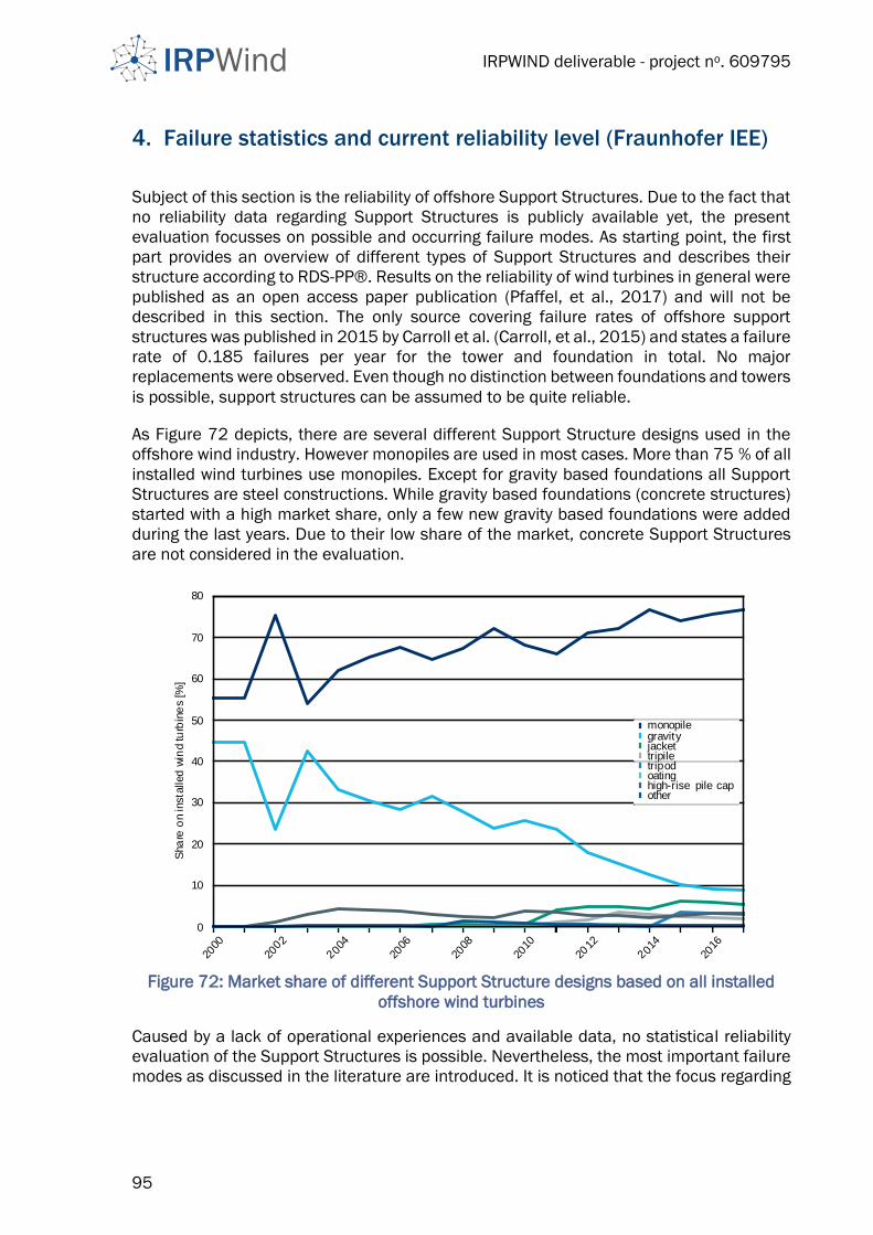
IRPWIND deliverable - project no. 609795
95
4. Failure statistics and current reliability level (Fraunhofer IEE)
Subject of this section is the reliability of offshore Support Structures. Due to the fact that
no reliability data regarding Support Structures is publicly available yet, the present
evaluation focusses on possible and occurring failure modes. As starting point, the first
part provides an overview of different types of Support Structures and describes their
structure according to RDS-PP®. Results on the reliability of wind turbines in general were
published as an open access paper publication (Pfaffel, et al., 2017) and will not be
described in this section. The only source covering failure rates of offshore support
structures was published in 2015 by Carroll et al. (Carroll, et al., 2015) and states a failure
rate of 0.185 failures per year for the tower and foundation in total. No major
replacements were observed. Even though no distinction between foundations and towers
is possible, support structures can be assumed to be quite reliable.
As Figure 72 depicts, there are several different Support Structure designs used in the
offshore wind industry. However monopiles are used in most cases. More than 75 % of all
installed wind turbines use monopiles. Except for gravity based foundations all Support
Structures are steel constructions. While gravity based foundations (concrete structures)
started with a high market share, only a few new gravity based foundations were added
during the last years. Due to their low share of the market, concrete Support Structures
are not considered in the evaluation.
Figure 72: Market share of different Support Structure designs based on all installed
offshore wind turbines
Caused by a lack of operational experiences and available data, no statistical reliability
evaluation of the Support Structures is possible. Nevertheless, the most important failure
modes as discussed in the literature are introduced. It is noticed that the focus regarding
2000
2002
2004
2006
2008
2010
2012
2014
2016
0
10
20
30
40
50
60
70
80
Sha
re o
n insta
lled w
ind tu
rbin
es [%
]
monopilegravityjackettripiletripodoatinghigh-rise pile capother
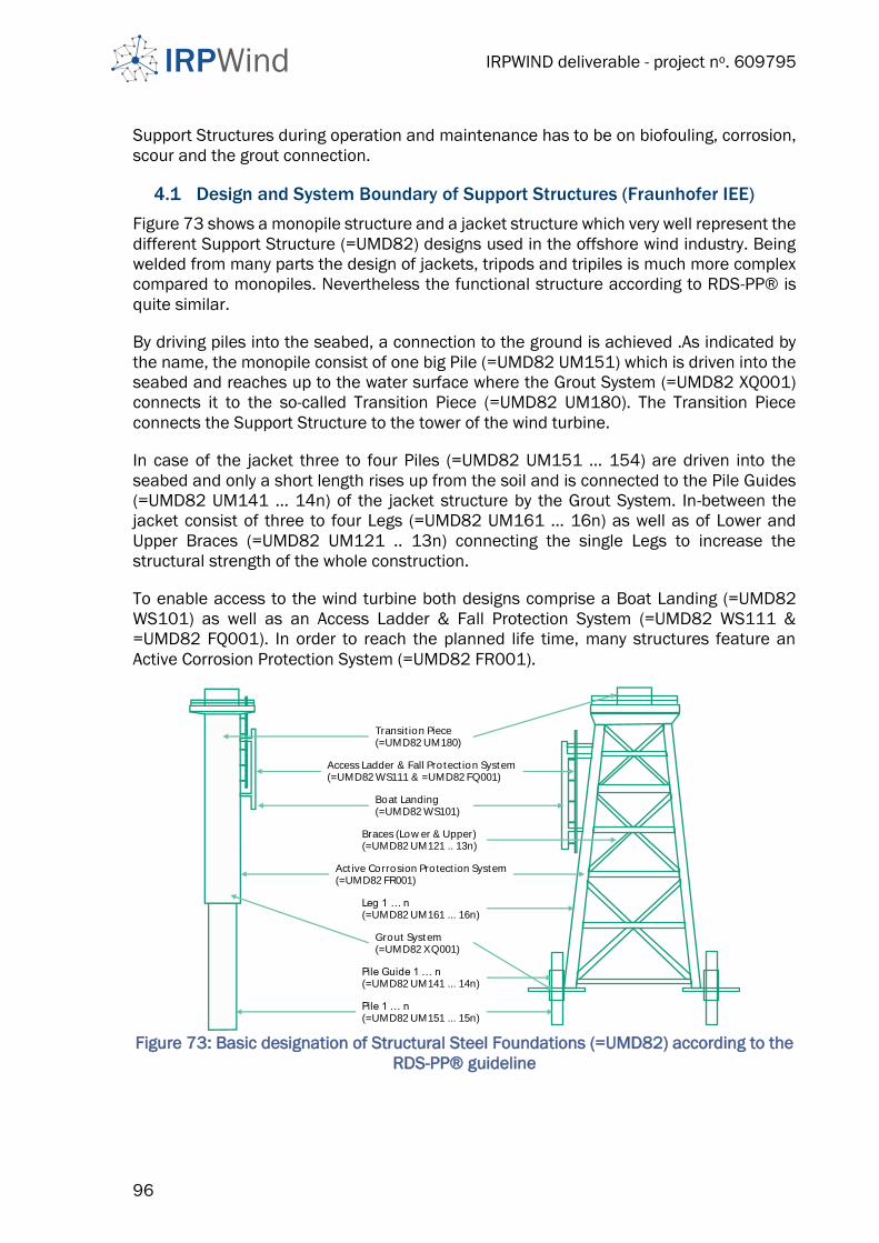
IRPWIND deliverable - project no. 609795
96
Support Structures during operation and maintenance has to be on biofouling, corrosion,
scour and the grout connection.
4.1 Design and System Boundary of Support Structures (Fraunhofer IEE)
Figure 73 shows a monopile structure and a jacket structure which very well represent the
different Support Structure (=UMD82) designs used in the offshore wind industry. Being
welded from many parts the design of jackets, tripods and tripiles is much more complex
compared to monopiles. Nevertheless the functional structure according to RDS-PP® is
quite similar.
By driving piles into the seabed, a connection to the ground is achieved .As indicated by
the name, the monopile consist of one big Pile (=UMD82 UM151) which is driven into the
seabed and reaches up to the water surface where the Grout System (=UMD82 XQ001)
connects it to the so-called Transition Piece (=UMD82 UM180). The Transition Piece
connects the Support Structure to the tower of the wind turbine.
In case of the jacket three to four Piles (=UMD82 UM151 … 154) are driven into the
seabed and only a short length rises up from the soil and is connected to the Pile Guides
(=UMD82 UM141 ... 14n) of the jacket structure by the Grout System. In-between the
jacket consist of three to four Legs (=UMD82 UM161 ... 16n) as well as of Lower and
Upper Braces (=UMD82 UM121 .. 13n) connecting the single Legs to increase the
structural strength of the whole construction.
To enable access to the wind turbine both designs comprise a Boat Landing (=UMD82
WS101) as well as an Access Ladder & Fall Protection System (=UMD82 WS111 &
=UMD82 FQ001). In order to reach the planned life time, many structures feature an
Active Corrosion Protection System (=UMD82 FR001).
Figure 73: Basic designation of Structural Steel Foundations (=UMD82) according to the
RDS-PP® guideline
Boat Landing(=UMD82 WS101)
Access Ladder & Fall Protect ion System(=UMD82 WS111 & =UMD82 FQ001)
Grout System(=UMD82 XQ001)
Act ive Corrosion Protect ion System(=UMD82 FR001)
Transit ion Piece(=UMD82 UM180)
Pile 1 … n(=UMD82 UM151 ... 15n)
Pile Guide 1 … n(=UMD82 UM141 ... 14n)
Leg 1 … n(=UMD82 UM161 ... 16n)
Braces (Low er & Upper)(=UMD82 UM121 .. 13n)
IRPWIND deliverable - project no. 609795
97
4.2 Failure Modes of Support Structures (Fraunhofer IEE)
The lifetime of Support Structures mainly depends on the different loads the structure has
to bear and is also influenced by environmental conditions such as wind, waves and
currents, UV radiation, salty water and salty air. (Heins, 2011) Support Structures are
designed to bear loads induced by the wind turbine through the tower as well as to
withstand loads due to wind and wave conditions. To ensure the structural integrity of the
Support Structure, it is required that design assumptions regarding the condition of the
structure persist. Known issues are biofouling, corrosion, scour and faulty grout
connections.
Loads on the tower, which are passed on to the Support Structure, are described in (Toft
& Sørensen, 2008) and caused by loads due to normal operation, by wake effects from
surrounding wind turbines and by extreme wind conditions. (Chella, et al., 2012) discuss
impact forces on the Support Structure due to waves. Experiences at the Fino 1 research
platform in the North Sea show that extreme waves are a real-world problem. During the
1st November 2006 the platform was hit by waves having significant wave heights of up
to 10.54 m. The storm caused heavy damage to a walkway where floor gratings were torn
from their mountings and also parts of the railings were heavily demolished. The Support
Structure (jacket) itself remained undamaged (Herklotz, n.d.).
These loads can be also influenced by vegetation (biofouling) growing on the surface of
the Support Structure which causes additional weight and leads to a change of the natural
frequency and drag due to an increased circumference of the Support Structure (Böttcher,
2013). At the research wind farm alpha ventus fouling biomass of about 25 kg per square
meter at a water depth of 1 m was found two years after installation while at water depth
of 5 m and 10 m fouling barely exceeded 1 kg per square meter. Based on experience
from the Fino 1 platform the authors expect a further weight increase at a water depth of
1 m while no mass grow is expected in deeper waters. (Gutow & etal, 2014)
The most important threat to the structural strength of steel-based Support Structures is
corrosion. Salty air and water as well as wetting-drying cycles make Support Structures
prone to corrosion. Thus corrosion protection is vital for Support Structures. To choose the
suitable corrosion protection systems, the Support Structure has to be divided into splash
zone, wet and dry zone and immersed zone. (Böttcher, 2013) and (Momber, et al., 2009)
Due to frequent contact to air and oxygen enriched seawater the splash zone and
especially welding seams show the highest corrosion potential (Ciang, et al., 2008). For
corrosion protection in the splash zone as well as in the wet and dry zone, various coating
systems (passive corrosion protection) are available and further research (e.g.
(WeserWind, B., 2015)) is carried out. Additional requirements to the coating systems
result from mechanical impact damages caused e.g. by docking workboats as well as by
scrubbing or loose and swinging parts. (DONG, 2009) Corrosion also occurs in sections
where the coating is missing or was not applied properly. According to (Momber, n.d.)
screws are also frequently affected by corrosion as well as sections of worn-out coatings
(e.g. walkways). (Momber, n.d.)
Within the immersed zone no coating is applied and the Support Structure is made of bare
steel. In this case active corrosion protection systems are utilized which can be either
based on a galvanic sacrificial anode (zinc or aluminum) as used at the EnBW Baltic 1

IRPWIND deliverable - project no. 609795
98
wind farm or realized as a cathodic corrosion protection using an external current as used
at the alpha ventus test site. In general corrosion protection systems are similar to
systems used in the shipping industry or the Oil & Gas sector (Heins, 2011).
Regarding the structural integrity of the Piles, scour is also an issue for Support Structures
due to increasing strains and a reduction of the natural frequency (Böttcher, 2013). As
van der Tempel shows (Tempel, 2006), lifetime fatigue damage is increasing with
increasing scour depth. In a worst case scenario deep scour can also threaten the stability
of the whole Support Structure. At the research wind farm alpha ventus scour depths of
at maximum 7.2 m (October 2013) were detected. After an rapid increase of the scour
depth during the first 3 to 5 months after installation, the later development continued
much slower (Kühn, 2013). Scour protection systems can be utilized to avoid or reduce
scour. One opportunity is to place rocks around the Support Structure which are to heavy
to be washed away (Tempel, et al., 2004). An alternative solution are geotextile sand
containers (Heerten & Peters, 2011). For monitoring purposes scour depths can be
evaluated using single beam or multi beam echosounder measurements (Kühn, 2013).
The Grout System connects on or more Piles to the rest of the Support Structure by filling
the distance between the inner and outer tube with cement. In 2009 slipping of grout
connections between monopiles and transition pieces was detected for the first time in
offshore wind (Lochte-Holtgreven & Bechtel, 2014). The offshore industry solved this
problem by installing additional elastomeric bearings at the concerned wind turbines. As
a preventive measure this solution is also installed at newly erected wind turbines (lorc.dk,
2012). Displacement sensors can be used to monitor the grout connection during
operation (Weijtjens, 2014).
With growing experience from operation and maintenance of offshore wind farms the main
impact factors and failure modes will be better understood and quantitative statements
for this critical structural component will be possible.

IRPWIND deliverable - project no. 609795
99
5. References
Achmus, M., 2011. Bemessung von Monopiles für die Gründung von Offshore-
Windenergieanlagen - Konzepte und offene Fragen. Bautechnik 88, pp. 602-616.
Achmus, M. & Müller, M., 2010. Evaluation of pile capacity approaches with
respect to piles for wind energy foundations in the North Sea. In: Frontiers in Offshore
Geotechnics Two. s.l.:CRC Press.
American Petroleum Institute, 2002. Recommended Practice for Planning,
Designing and Constructing Fixed Offshore Platforms - Working Stress Design.
Recommended Practice RP 2A-WSD, s.l.: s.n.
American Petroleum Institute, 2014. Geotechnical and Foundation Design, s.l.: s.n.
API, 2007. Errata and Supplement 3 – API Recommended Practice 2A-WSD,
Recommended Practice for Planning, Designing, Constructing Fixed Offshore Platforms –
Working Stress Design, s.l.: s.n.
Bea, R. G., Jin, Z., Valle, C. & Ramos, R., 1999. Evaluation of Reliability of Platform
Pile Foundations. Journal of Geotechnical and Geoenvironmental Engineering, 128(8), pp.
696-704.
Böttcher, J., 2013. Jörg , Handbuch Offshore-Windenergie: Rechtliche, technische
und wirtschaftliche Aspekte, s.l.: s.n.
BOWNESS, D. & M.M.K., L., 2002. Fracture mechanics assessment of fatigue
cracks in offshore tubular structures. HSE Offshore Technology Report 2000/077 for
HSE, EPSRC, and Chevron Oil., London: The Stationery Office.
BS 7910, 2013. Guide to methods for assessing the acceptability of flaws in
metallic structures., London: British Standards Institution.
Carroll, J., McDonald, A. & McMillan, D., 2015. Failure rate, repair time and
unscheduled O&M cost analysis of offshore wind turbines. Wind Energy.
Cathie, D., 2012. Offshore pile design according to international practice. s.l.:Free
published presentation.
CEB-fip, 2013. fib Model Code for concrete structures2010. Lausane: Ernst & Son.
Chella, M. A., A., T. & Myrhaug, D., 2012. An Overview of Wave Impact Forces on
Offshore Wind Turbine Substructures. Energy Procedia, Volume 20, p. 217–226.
Chen, J.-Y. & Gilbert, R., 2014. Insights into the Performance Reliability of Offshore
Piles Based on Experience in Hurricanes. From Soil Behavior Fundamentals to Innovations
in Geotechnical Engineering, pp. 283-292.
Chen, J.-Y.et al., 2009. Analyses of Pile Capacity for Offshore Structures in
Hurricane Katrina. Contemporary Topics in Deep Foundations, ASCE, pp. 239-246.
Ciang, C. C., Lee, J.-R. & Bang, H.-J., 2008. Structural health monitoring for a wind
turbine system: A review of damage detection methods. Meas. Sci. Technol., 19(12), p.
122001.
Cornelissen, H. A. W., 1984. Fatigue Failure of Concrete in Tension, Delft: HERON.
Craig Jr., R. R. & Bampton, M. C. C., 1968. Coupling of Substructures for Dynamic
Analyses. AIAA Journal 6 (7), pp. 1313-1319.
Dallyn, P., El-Hamalawi, A., P. A. & K. R., 2015. Experimental testing of grouted
connections for offshore substructures: A critical review.. Structures, Volume 3, pp. 90-
108.
Damiani, R., Jonkman, J., Robertson, A. & Song, H., 2013. Assessing the
Importance of Nonlinearities in the Development of a Substructure Model for the Wind
Turbine CAE Tool FAST. Nanted, s.n.

IRPWIND deliverable - project no. 609795
100
De Wries, W. & et.al, 2011. Support Structure Concepts for Deep Water Sites.
UpWind Project Deliverable Report D4.2.8, s.l.: UpWind.
DIN 1054, 2010. Baugrund-Sicherheitsnachweise im Erd und Grundbau, s.l.:
Deutsches Institut für Normung.
DIN EN 61400-3, 2010. Windenergieanlagen - Teil 3-1: Auslegungsanforderungen
für Windenergieanlagen auf offener See, s.l.: Deutsches Institut für Normung.
Dithinde, M., Phoon, K., DeWet, M. & Retief, J., 2011. Characterization of the Model
Uncertainty in the Static Pile Design Formula. Journal of Geotechnical and
Geoenvironmental Engineering, 137(1), pp. 70-85.
DNV GL, 2015. RP-C 210. Probabilistic methods for planning of inspection for
fatigue cracks in offshore Structures.. s.l., DNVGL.
DNVGL-RP-0419, 2016. Analysis of grouted connections using the finite element
method – Recommended Practice., Copenhagen: Det Norske Veritas.
DNVGL-ST-0126, 2016. Support structures for wind turbines, s.l.: DNVGL.
DNVGL-ST-C502, 2017. Offshore Concrete Structures, s.l.: DNVGL.
DNV-RP-C203, 2011. Fatigue Design of Offshore Steel Structures, Recommended
practice, s.l.: Det Norske Veritas.
DONG, 2009. Korrosionsschutz in der maritimen Technik, Copenhagen: Wind Kraft
Journal.
Eurocode 0, 2010. DIN EN 1990: Eurocode: Grundlagen der Tragwerksplanung,
s.l.: Deutsches Institut für Normung.
European Committee for Standardization, 2010. Eurocode 3: Design of steel
structures – Part 1-9: Fatigue, s.l.: EN 1993-1-9.
Germanischer Lloyd, 2005. Rules and Guidelines, IV Industrial Services, Guideline
for the Certification of Offshore Wind Turbines, s.l.: Germanischer Lloyd Wind Energie
GmbH.
Gilbert, R. & Tang, W., 1995. Model Uncertainty in Offshore Geotechnical
Reliability. Houston, USA, s.n.
Guyan, R. J., 2065. Reduction of stiffness and mass matrices. AIAA journal 3.2, p.
380.
Gutow, L. & etal, 2014. Rapid increase of benthic structural and functional
diversity at the alpha ventus offshore test site,” in Ecological research at the Offshore
Windfarm alpha ventus: Challenges, results and perspectives,, Wiesbaden: Springer.
Häckel, M. & Rolfes, R., 2013. Monitoring a 5MW offshore wind energy converter-
Condition parameters and triangulation based extraction of modal parameters.
Mechanical Systems and Signal Processing, 40(1), pp. 322-343.
Häfele, J., Hübler, C., Gebhardt, C. G. & Rolfes, R., 2016. An improved two-step soil-
structure interaction modeling method for dynamical analyses of offshore wind turbines.
Applied Ocean Research, 55, pp. 141-150.
Häfele, J., Hübler, C., Gebhardt, C. G. & Rolfes, R., 2017. A comprehensive fatigue
load set reduction study for offshore wind turbines with jacket substructures. Renewable
Energy.
Häfele, J., Hübler, C., Gebhardt, C. G. & Rolfes, R., 2017. Efficient Fatigue Limit
State Design Load Sets for Jacket Substructures Considering Probability Distributions of
Environmental States. San Francisco, s.n.
Hald, T. et al., 2009. Revisiting monopile design using py curves. Results from full
scale measurements on Horns Rev. s.l., s.n.
Hansen, M. et al., 2015. Probabilistic Safety Assessment of Offshore Wind
Turbines (PSA-OWT), s.l.: Leibniz Universität Hannover.

IRPWIND deliverable - project no. 609795
101
Heerten, G. & Peters, K., 2011. Kolkschutz für Offshore-Windenergieanlagen in der
Nordsee. geotechnik, 34(1), p. 51–58.
Heins, O., 2011. Korrosionsschutz von Offshore-Windenergieanlagen: Einteilung,
Normung und praktische Erfahrungen.. [Online]
Available at: http://www.htg-
online.de/fileadmin/user_upload/korrosionsfragen/downloads/HTG-
Kongress_Wuerzburg_09-09-2011/HTG-2011_Korrosion
Herklotz, K., n.d. Oceanographic Results of Two Years Operation of the First
Offshore Wind Research Platform in the German Bight - FINO1., s.l.: s.n.
Holicky, M., Markova, J. & Gulvanessian, H., 2007. Code Calibration Allowing for
Reliability Differentiation and Production Quality. London, s.n.
Hübler, C., Gebhardt, C. G. & Rolfes, R., 2017. Development of a comprehensive
database of scattering environmental conditions and simulation constraints for offshore
wind turbines. Wind Energy Science, pp. 491-505.
Hübler, C., Gebhardt, C. G. & Rolfes, R., 2017. Hierarchical Four-Step Global
Sensitivity Analysis of Offshore Wind Trubines Based on Aeroelastic Time Domain
Simulations. Renewable Energy.
Hübler, C., Gebhardt, C. G. & Rolfes, R., 2018. Methodologies for fatigue
assessment of offshore wind. Wind Energy.
Hübler, C., Häfele, J., C.G., G. & Rolfes, R., 2018. Experimentally supported
consideration of operating point dependent soil properties in coupled dynamics of
offshore wind turbines. Marine Structures, p. 18e37.
Hübler, C., Häfele, J., Ehrmann, E. & Rolfes, R., 2016. Effective consideration of
soil characteristics in time domain simulations of bottom fixed offshore wind turbines.
Rhodos, s.n.
Hübler, C., Müller, F., Gebhardt, C. G. & Rolfes, R., 2017. Global Sensitivity Analysis
of Offshore Wind Turbine Substructures. Dresden, s.n.
Yang, Z., Jardine, R., Guo, W. & Chow, F., 2015. A new openly accessible database
of tests on piles driven in sands. Géotechnique Letters, Volume 5, pp. 12-20.
IEC 61400-1, 2017. IEC 61400-1. Wind turbines – Part 1: Design requirements.
4th edition, Geneva: IEC.
IEC 61400-6, 2017. IEC 61400-6 Wind Energy Generation Systems – Part 6: Tower
and Foundation Design Requirements, Geneva: FDIS .
International Electrotechnical Commision, 2009. Wind turbines - Part 3. 2009.
Design requirements for offshore wind turbines, Standard IEC-61400-3:2009, EN 61400-
3, s.l.: s.n.
Jamiolkowski, M., Ghionna, V., Lancellotta, R. & Pasqualini, E., 1988. New
Correlations of Penetration Tests for Design Practice. Orlando, s.n.
Jardine, R., Chow, F., Overy, R. & Standing, J., 2005. ICP design methods for driven
piles in sands and clays. London: Thomas Telford Publishing.
JCSS , 2012. Probabilistic Model Code - PART 3.12 Fatigue properties for metallic
structures. Draft ., s.l.: Joint Commitee for Structural Safety.
Jonkman, J., 2013. The New Modularization Framework for the FAST Wind Turbine
CAE Tool. 51st AIAA Aerospace Sciences Meeting, including the New Horizons Forum and
Aerospace Exposition.
Jonkman, J., Butterfield, S., Musial, W. & Scott, G., 2009. Definition of a 5MW
Reference Wind Turbine for Offshore System Development, s.l.: National Renewable
Energy Laboratory.
IRPWIND deliverable - project no. 609795
102
Jonkman, J. & Musial, W., 2010. Offshore Code Comparison Collaboration (OC3)
for IEA Task 23 - Offshore Wind Technology and Deployment. Tech. Rep. NREL/TP-5000-
48191, s.l.: National Renewable Energy Laboratory.
Jonkman, J. et al., 2012. Offshore Code Comparison Collaboration Continuation
(OC4), Phase I - Results of Coupled Simulations of an Offshore Wind Turbine with Jacket
Support Structure. Rhodos, s.n.
Kallehave, D., LeBlanc Thilsted, C. & Liingaard, M., 2012. Modification of the API
p-y formulation of initial stiffness of sand.. London, s.n.
Kirsch, F., Richter, T. & Coronel, M., 2014. Geotechnische Aspekte bei der
Gründungsbemessung von Offshore-Windenergieanlagen auf Monopfählen mit sehr
großen Durchmessern. Ernst & Sohn Verlag für Architektur und technische
Wissenschaften GmbH & Co. KG, Berlin · Stahlbau Spezial 2014 – Erneuerbare Energien.
Kühn, B., 2013. Geological research at alpha ventus: The spatiotemporal
development of scours., s.l.: Alpha Ventus.
Kulhawy, F. & Mayne, P., 1990. Manual on Estimating Soil Properties for
Foundation Design. s.l.:Electric Power Research Institute.
Lantsoght, E., 2014. Fatigue of concrete under compression - Database and
proposal for high strength concrete.Report nr. 25.5-14-04, Delft: Delft University of
Technology.
Lehane, B., Schneider, J. & Xu, X., 2005. review of design methods for offshore
driven piles in siliceous sand, s.l.: University of Western Australia Geomechanics Group.
Lindley, D. V., 1976. Introduction to Probability and Statistics from a Bayesian
Viewpoint, Vol. 1_2. Cambridge: Cambridge University Press.
Lochte-Holtgreven, S. & Bechtel, A., 2014. Grout-Verbindungen in Monopile-
Tragstrukturen von Offshore-Windenergieanlagen. Stahlbau, 83(4), pp. 273-277.
lorc.dk, 2012. Overcoming problems with crumbling grout.. [Online]
Available at: http://www.lorc.dk/oceanwise-magazine/archive/2012-2/overcoming-
problems-with-crumbling-grout
Lotsberg, I., 2013. Structural mechanics for design of grouted connections in
monopile wind turbine structures.. Marine Structures, Volume 32, p. 113–135.
Madsen, C., Kragh-Poulsen, J., Thage, K. & Andreassen, M., 2017. Analytical and
numerical investigation of bolted steel ring flange connection for offshore wind monopile
foundations”. Stavanger, Norway, First Conference of Computational Methods in Offshore
Technology.
Momber, A., n.d. Inspektion und Reparatur von Offshore-Wind-Konstruktionen, s.l.:
Muehlhan AG.
Momber, A., Plagemann, P., Stenzel, V. & M., S., 2009. Beurteilung von
Korrosionsschutzsystemen für Offshore-Windenergietürme - Teil 1: Problemstellung und
Versuchsdurchführung. Stahlbau, 78(4), pp. 259-266.
Natarajan, A. & Holley, W., 2008. Statistical extreme load extrapolation with
quadratic distortions for wind turbines.. Journal of solar Energy Engineering (031017) ,
Volume 130, pp. 1-7.
Pfaffel, S., Faulstich, S. & K., R., 2017. Performance and Reliability of Wind
Turbines: A Review. Energies, 10(11), p. 1904.
Phoon, K. & Kulhawy, F., 1999. Characterization of geotechnical variability.
Canadian Geotechnical Journal, Volume 36, pp. 612-624.
Rodriguez, A. et al., 2018. DEVELOPMENT OF NEW METHODOLOGIES TO ASSESS
THE STRUCTURAL INTEGRITY OF THE GROUTED JOINT OF A 10 MW WIND TURBINE
SUBSTRUCTURE. Madrid, OMAE, p. 12.
IRPWIND deliverable - project no. 609795
103
Saltelli, A. et al., 2008. Global sensitivity analysis: the primer. s.l.:John Wiley &
Sons.
Santos, B. et al., 2017. D7.21. Report on Validation of design of grouted joints,
Brussels: IRPWIND.EU.
Schaumann, P., Lochte-Holtgreven, S. & Eichstadt, R., 2013. Numerical
investigation on local degradation and vertical misalignment of grouted joint in monopile
foundations.. Anchorage, Alaska, USA., ISOPE 2013.
Schittkowski, K., 1986. NLPQL: A FORTRAN Subroutine Solving Non-Linear
Programming Problems. Ann. Operat. Res., 5, p. 485–500.
Schmoor, K., 2017. Probabilistische Analyse zum Sicherheitsniveau von Offshore-
Gründungspfählen (PhD Thesis), s.l.: Institute for Geotechnical Engineering, Leibniz
University Hannover.
Schneider, J., Xu, X. & Lehane, B., 2008. Database Assessment of CPT-Based
Design Methods for Axial Capacity of Driven Piles in Siliceous Sands. Journal of
Geotechnical and Geoenvironmental Engineering, 134(9), pp. 1227-1244.
Simpson, B., 2012. Eurocode 7: Fundamental issues and some implications for
users. s.l., s.n.
Slot, R. & Andersen, T., 2014. Fatigue behavior and reliability of high strength
concrete. MSc thesis, Aalborg: Aalborg University.
Sørensen, J. & Toft, H., 2014. Safety Factors – IEC 61400-1 ed. 4 - background
document., Copenhagen: DTU Wind Energy.
Sørensen, S., 2012. Soil-structure interaction for non-slender, large-diameter
offshore monopiles. PhD Thesis, Aalborg University Denmark, Department of Civil
Engineering: s.n.
Sørensen, S. P. H., Ibsen, L. B. & Augustesen, A. H., 2010. Effects of diameter on
initial stiffness of py curves for large-diameter piles in sand. Numerical Methods in
Geotechnical Engineering.
Tempel, J. v. d., 2006. Design of support structures for offshore wind turbines. [S.l.:
s.n.], op. 2006., s.l.: s.n.
Tempel, J. v. d., Zaaijer, M. & Subroto, H., 2004. The effects of Scour on the design
of Offshore Wind Turbines., Delft: TU Delft.
Thieken, K., Achmus, M. & Lemke, K., 2015. A new static p-y-approach for piles
with arbitrary dimensions in sand. Geotechnik 38 (4).
Toft, H. S. & Sørensen, J. D., 2008. Reliability Analysis of Wind Turbines, Aalobrg:
Aalborg unversity.
VanOverschee, P. & DeMoor, B., 1991. Subspace algorithms for the stochastic
identification problem. Decision Control, Volume 2, p. 1321–1326.
Wandji, W., Natarajan, A. & Dimitrov, N., 2018. Probabilistic structural assessment
of conical grouted joint using numerical modelling.. Journal of Ocean Engineering, p.
Under Review.
Weijtjens, W. e., 2014. Monitoring of offshore turbines for design and O&M: an
overview of the activities of OWI-Lab, s.l.: OWI-Lab.
WeserWind, B., 2015. KOWIND, Hannover: TIB - Technische Informationsbibliothek
Universitätsbibliothek Hannover.
Wiemann, J., Lesny, K. & Richwien, W., 2004. Evaluation of the Pile Diameter
Effects on Soil-Pile Stiffness. s.l., s.n.
Zaaijer, M. B., 2006. Foundation modelling to assess dynamic behaviour of
offshore wind turbines. Applied Ocean Research 28.1, pp. 45-57.
IRPWIND deliverable - project no. 609795
104
Zwick, D. & Muskulus, M., 2015. The simulation error caused by input loading
variability in offshore wind turbine structural analysis. Wind Energy, Issue 18, pp. 1421-
1432.