AAS 12-190

A VISUAL ANALYTICS APPROACHTO PRELIMINARY TRAJECTORY DESIGN

Wayne R. Schlei∗, Kathleen C. Howell†

Recent developments in astrodynamics suggest a wealth of design potential within the con-text of the circular restricted three-body problem. Exploitation of the expanding dynamicaland mathematical insights, though, has been difficult to capture within a real-time designsetting. Emerging from the ability to represent large amounts of information through visualenvironments, visual analytics is a new science that focuses on the application of graphicaldepictions to facilitate discovery. Moreover, visual analytics blends the science of analyt-ical reasoning with the implementation of interactive visual interfaces. In considering themost effective approach to incorporate visual elements in a largely automated process, thisinvestigation blends the fundamentals of trajectory design in multi-body regimes with theimplementation of visual analytics, thereby merging visualization tools, differential correc-tions algorithms, and the intuition of a knowledgeable designer into one expansive designapproach. Visual analytics offers a basis for rapid investigation and design with access to awider range of options for the construction of trajectories that meet mission requirements.

INTRODUCTION

Computer-generated visualizations offer an exceptionally powerful tool for the understanding of mathe-matical concepts and spatial relationships. In spacecraft trajectory design, visualization is frequently a keyto success. In recent years, commercial software packages have emerged, such as Satellite Tool-Kit R© , thatsupport trajectory development with adaptable three-dimensional (3D) views and spacecraft flight animationsfrom the perspective of a variety of coordinate frames.1 Recent advances in trajectory analysis for vehiclesunder the influence of multiple gravitational fields offer innovative concepts for scientific exploration, espe-cially within the context of the Circular Restricted Three-Body Problem (CR3BP). Exploiting the dynamicalstructures available in multi-body regimes, such as the CR3BP, is very appealing for design scenarios, and,in fact, much effort is currently focused on developing numerical capabilities to enable faster adaptive designstrategies. But effectively exploiting such structures within an interactive visual design environment remainsan intriguing challenge. The best balance between automated computation and visual insights can be elusive.

In recent years, the emergence of visual analytics, a science that merges the intuition of humans withscientific visualization and interactive environments, assists researchers from various fields in solving multi-dimensional problems and examining complex systems. Astronomers and astrophysicists, for example, in-corporate visual analytics while producing three-dimensional (3D) simulations of a supernova core collapseto analyze patterns in the plethora of output parameters from such an event including turbulence, rotation,radiation, magnetic fields, and gravitational forces.2 In fact, visual analytics is often employed to extractinformation and insight from large quantities of unstructured data, but visual analytics can also be incorpo-rated in support of design decisions in the engineering realm. With visual analytics applied in the automotiveindustry, engineers interactively alter vehicle construction schemes and various parameters during 3D flowsimulations to optimize air resistance or engine efficiency.2 A design approach incorporating visual analyticsis analogous to an interactive computer-aided design (CAD) application for drafting mechanical parts. For∗Ph.D. Student, Purdue University, School of Aeronautics and Astronautics, 701 West Stadium Avenue, West Lafayette, Indiana 47907-

2045.†Hsu Lo Professor of Aeronautical and Astronautical Engineering, Purdue University, School of Aeronautics and Astronautics, 701 WestStadium Avenue, West Lafayette, Indiana 47907-2045.

1

example, a mechanical designer uses the visual interface in a CAD package to sketch geometries, generate 3Drepresentations of parts, and test-fit a product assembly. The visual interactive CAD tool offers a mechanicaldesigner the ability to quickly assess the parts and the mechanical functionality based on visual feedback and,then, to interactively modify components to meet a variety of requirements.3

In seeking a more automated trajectory design process, the most effective strategy to incorporate the visualelements is explored. Visual analytics may offer a framework. For example, the use of visualization simply inpost-processing offers only visual comprehension. However, the rendering of a scene requires that data rep-resenting graphics primitives (triangles, polygons, objects) is accessible for culling or lighting operations.3

A visual analytics design application can utilize this same information with human interaction; the visualinterface can be exploited to construct and manipulate initial guess arcs for potentially seeding a differentialcorrections process thereby assisting efficiency in the trajectory design process. Furthermore, if the cor-rections process is implemented within the same graphical interface, the preliminary trajectory constructionand analysis occurs instantly. In short, visual analytics combines interactive computation and a knowledgebase with trajectory visualization and other scientific visual techniques, creating an interactive approach forgenerating solutions and allowing other design options.

Previous Contributions in Trajectory Design

One commercial package that is available for spacecraft trajectory design in libration point missions isSatellite Tool-Kit R© (or STK R© made by Analytical Graphics, Inc.), which includes a visual component. BothSTK R© and its predecessor Swingby have been successfully employed during the design phase and for flightoperations in support of various libration point missions including Wind, SOHO, ACE, MAP, and CON-TOUR.1 The STK R© developers and users continually emphasize the advantages of design analysis with im-mediate visual feedback. The communication of trajectory concepts is greatly enhanced with 3D imageryand animations.1 Design within the context of the CR3BP also offers an opportunity to apply dynamicalsystems and orbit stability analysis tools. For example, the role of invariant manifolds and their applicationsto trajectory design are introduced by various investigators including Lo, Anderson, et al.,4–6 and the effectiveuse of Poincare maps for trajectory design applications is demonstrated by numerous researchers.6–8

Some previous investigations introduce elements of visual analytics into the analysis of design problems.For instance, to transfer from a specified low-Earth orbit to a Sun-Earth L1 halo orbit, Museth, Barr, andLo use a 3D workbench with an immersive interface to select a suitable arc along a stable manifold basedon visual inspection.9 The resulting transfer arc is then employed as part of the design for the ‘TerrestrialPlanet Finder’ mission.9 The implementation by Museth, Barr, and Lo introduces the visual design concept;however, more extensive functionality is directly available through a visual design approach. The purpose ofthe application of visual analytics to the spacecraft trajectory design problem is the potential to introduce themost recent theoretical developments into the design process as quickly and effectively as possible. In thecurrent effort, the goal is the exploitation of advanced dynamical systems theory to generate solutions thatmeet specific trajectory design objectives that may be difficult to quickly achieve otherwise. As a designeror analyst, the goal is the most effective use of this new wealth of visual information while simultaneouslyshifting towards a more automated design approach.

Current Work

The design and construction of spacecraft trajectories in multi-body environments may be enhanced withthe application of a visual analytics framework. The use of visualization is more than a simple display ofthe trajectory information; it also supplies trajectory development tools and new information concerningthe dynamical models. Implementing user-built computation modules and interaction functions with visualinterfaces allows the user to analyze the available information and immediately adjust the data, visualization,or computation processes. The visual elements can, in fact, support the automated processes. As a potentialstrategy, this investigation offers a blend of spacecraft trajectory design with visual analytics, thereby mergingvisualization tools, numerical algorithms, and designer intuition into one design approach.

2

VISUAL ANALYTICS

With the advent of advanced computer graphics and rapid rendering software and technologies, the abilityto represent large amounts of information through visual environments has evolved. Thus, a new scienceborn of this ability focuses on the effective application of graphical depictions to facilitate discovery. Visualanalytics blends the science of analytical reasoning with the implementation of interactive visual interfaces.10

Keim et al. define visual analytics more precisely as “an interactive process that involves information gath-ering, data preprocessing, knowledge representation, interaction and decision making”.2 The computing andvisualization power of machines combined with the decision-making abilities of humans leads to knowledgediscovery that may not be available through standard analytical tools.2 The application of visual analyticsto spacecraft trajectory design supplies an immensely powerful tool in research and development as well asenhanced capabilities to produce a wider range of options for trajectories to meet mission requirements. Moreeffective use of the visual components can significantly aid a trajectory analyst.

The Visual Analytics Process

Understanding the application of visual analytics to trajectory design begins with a detailed description ofthe visual analytics process. The goal of this process is an innovation or insight, I , based on some initial inputdata, S. Three phases of analysis exist in transforming S to I , including analytical abstractionsA, hypothesesH , and visualizations V . All the component functions and their interactions are demonstrated in Figure 1,which is a diagram of the visual analytics process.2, 11, 12 The analytical abstraction phase, identified by thegray rectangle in Figure 1, involves tailoring the input data into manageable or relevant blocks through datamanipulation techniques and the applications of theory. Characterized by the purple rectangle in Figure 1, thehypothesis phase reflects a type of confirmation analysis in the form of a supposition that is evaluated, similarto a hypothesis in the standard scientific method. However, in the visual analytics process, the affirmationof new ideas is drawn from visual components along with previously existing theory and data. Thus, thecore of the visual analytics process is the implementation of the visualization phase. This visualizationphase, represented by a blue box in Figure 1, incorporates elements of scientific visualization, informationvisualization, and the cognitive and perceptual sciences as well as graphical interfaces for visual explorationof information. Overall, the visual analytics process is more encompassing than simply the application ofvisualization methods. It is actually a coalescence between visualization, human cognition and interaction,as well as theoretical and data analysis.2

Input Data (S)

Feedback Loop (G)

VU

VHHV

HU

CHU

CVUSV

AV

AH

WA

Visualization (V)

Hypothesis (H)

Analytical Abstraction

(A)

Innovationor Insight

(I)

AU

Figure 1. Diagram of the visual analytics process (adapted from2, 11, 12).

3

Fundamentally, visual analytics transforms an input S to an insight I . Thus, the visual analytics process isformally represented by the mapping function F : S 7→ I . The over-arching transformation F consists of aset of sub-functions f , where f ∈ {AW , VX , HY , UZ}. This set maps the visual analytics process from onephase to another as illustrated by Figure 1. The subscripts W , X , Y , and Z are used as shorthand notationto symbolize different types of functions utilized in each member of the set f . Thus, each member of f is afurther subset of functions that are described by the following:

• FunctionsAW : Data preprocessing and theoretical analysis tools reside in the set of functionsAW thatmap the input data to an analytical abstraction (i.e., AW : S 7→ A). The subscript W symbolizes eachtype of function available in the mapping from S to A, such that W ∈ {T,C, L, Th}. Transformationsof data are contained in AT , data cleaning operations reside in AC , AL represents functions used toselect specific sub-sections of the input data, and the applications of analytical theory are included inATh.

• Functions VX : The set VX , where X ∈ {S,A,H}, denotes the employable visualization functions.Visualizing the data directly is performed with the mapping VS : S 7→ V , an analytical abstraction isviewed via VA : A 7→ V , and VH : H 7→ V represents the transfer function denoting the visualizationof a hypothesis. These visualization functions cover rudimentary computer graphics procedures (e.g.,representing a point as a sphere or viewing axes and flow meshes as grids) and embrace any knownscientific or information visualization algorithms.

• Functions HY : The formation of a hypothesis occurs within the functions HY , where Y ∈ {A, V }.Hypotheses generated from analytical abstractions of the input data S are symbolized byHA : A 7→ H .Then, HV characterizes a hypothesis derived directly from a visualization (HV : V 7→ H).

• Functions UZ: User interaction in the visual analytics process is represented with the functions UZ ,each sub-function identified by Z ∈ {A,H, V,CV,CH}. These interactive functions consist of ei-ther direct interaction with an object existing within a visual environment or as a decision-makingcomponent. The set of functions UA : A 7→ A includes all selections or alterations a user imple-ments with an analytical abstraction. A hypothesis can be modified by the user through the functionUH : H 7→ H . Adjustments to a visualization via human interaction are represented by functionslinked with UV : V 7→ V . Basic camera operations like zooming, panning, or view reorientation,alterations to graphical object properties such as color and transparency, as well as lighting styles areall associated with UV . The desired output of the entire process, i.e., the insight I , is then deduced asthe output from either the visualization (UCV : V 7→ I) or hypothesis (UCH : H 7→ I) phases.

The steps from S to I are then modeled in terms of these components.

The entire visual analytics process is recursive, based on the user-specified level of detail. The outputof this process, or the realization of the insight I , may sometimes suggest that either further knowledge isavailable or more detail is required to be sufficient to render a conclusion. If so, modifications of an individualphase or a different set of transfer functions are derived given the current level of insight. In such a scenario,the process restarts with a feedback loop, G, that maps the achieved insight I back to new input data S(G : I 7→ S). The feedback function G also appears in Figure 1. This feedback loop reflects an update tothe input, that is, a modification of the input data S resulting from a discovery. (For more information on thevisual analytics process and applications, see Keim et al.,2 Risch et al.,11 or Huang and Ngyuen.12)

Selection of an Interactive Visualization Software

Visualization software options are expanding rapidly. In addition, computational software that offers visualsupport is widely available including packages for astrodynamics applications. For this investigation, moreextensive access to interactive visualization capabilities is necessary since user interactions are an integralpart of the visual analytics process.2 Interactive visual explorations require a visual environment capableof fast navigational changes, such as zooming, panning, and reorientation of the camera, to grasp spatiallocation and the depth of objects in a three-dimensional (3D) scene.11, 12 Also, real time human-computer

4

interaction involves visualization algorithms capable of processing hundreds of thousands of visual modifica-tions in seconds to be useful for knowledge discovery (with a maximum of only a few minutes).12 If a slightmodification is desired, for instance, a change in coloring, the individual objects must be modified quickly– inside the visual environment – for real-time knowledge discovery. Thus, the visualization software mustpossess the dexterity to implement quick modifications of a scene. Any sort of data computation involvedwith the analytical abstraction phase is also subject to the same speed requirements for real-time insight. Itis likely that user-built functions are responsible for abstracting or analyzing a specific substructure of thedata, but the visualization tool may also incorporate some computational components that support this con-cept. The scientific visualization suite Avizo R© from Visualization Sciences Group (VSG) is one particularvisualization package that offers the versatility to supply all of the required elements of the visual analyticsprocess. Stalling et al. state that Avizo R© is built with flexibility, interactivity, and extensibility as designgoals.13 Avizo R© incorporates a variety of different data types with the ability to visualize and perform oper-ations with multiple data sets simultaneously. It also houses an enriched interactive capability with 2D and3D environments. Human interaction with a visual scene is accomplished by using picking functions anddragger objects that are built using Open Inventor R©. Information about points, a mesh grid, or the faces of asurface, as well as any associated data values, are obtained by simply clicking.13 Thus, Avizo R© serves as thebasis for the visualizations in this analysis.

The Visual Analytics Process Applied to Trajectory Design

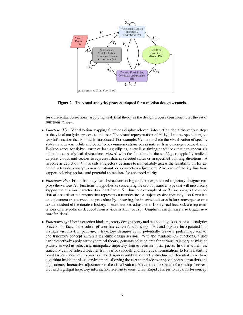
The visual analytics process is adapted from the general process in Figure 1 to accommodate the variouselements of a sample trajectory design scenario. First, the mission parameters and requirements supersede theinput data, S, as the starting point in the visual analytics process. Examples of possible trajectory parametersinclude predetermined starting or ending conditions, timing conditions, and known mission objectives eitheroperational or scientific in origin such as rendezvous, landing, desired ground tracks, or predetermined orbits.Figure 2 indicates mission parameters by the red component that initiates the visual analytics process. Forthe analytical abstraction phase, A, the trajectory design supplement represents the subdivision of a missioninto pertinent phases, the selection of a dynamical model for propagation, the application of known dynamicaltheory, as well as the formulation and execution of corrections or computational procedures. The visualizationphase, V , contains all the available graphical possibilities for points, vectors, and paths as well as any otherscientific visualization procedures applicable to trajectory design. During the hypothesis phase, H , possibleorbits or transfer arcs that may meet mission criteria are proposed. Any adjustments to the corrections processare also theorized during the hypothesis phase. The resulting insight, I , is then a partial path or the completespacecraft trajectory. As in the original form of the visual analytics process, I might also include discoveredknowledge such as some particular behavior associated with a dynamical model. It is possible that a resultingtrajectory, I , may not meet the mission requirements set forth by S. In such a case, a feedback loop, G,adjusts A, V , or H to determine a viable path. Finally, G can also modify S if the constraints on the designare infeasible.

The functions mapping one visual analytics phase to another phase now apply to direct trajectory designprocedures. The interplay between the visual analytics mapping functions and trajectory design appears ineach of the function types:

• Functions AW : The set of functions AW map mission and/or trajectory parameters into useful analyt-ical abstractions. Note that S may also contain any discovered trajectory or insight (I) from a previousapplication of the visual analytics process. Each particular subfunction in the set AW represents rele-vant trajectory design procedures. The AT functions modify states using spatial transformations suchas translation, rotation, and scale, or the functions can extract the velocity states of a trajectory forexamination in a phase space. Moreover, AT functions map trajectory constraints into the differentialcorrections process; functions in this set also alter selected states in position, velocity, and time throughthe execution of a differential corrections algorithm. The removal of states, arcs, constraints, and mis-sion objectives are types of data cleaning operations, AC . The subset of functions in AL are associatedwith the selection of subsets of data; functions in the set AL can separate a mission into phases, isolatea particular phase for analysis, select a specific arc from a group or family, or abstract patch points

5

Mission Param.

(S)

Adjustments to S, A, V, or H (G)

VU

VH

HV

HU

CHU

CVUSV

AV

AH

WA

Visualizing Mission Elements &

Trajectories (V)

Transfer Possibilities, Correction Adjustments

(H)

Subdivision,Model Selection,

Dynamical Theory, Corrections (A)

Resulting Trajectory,

Mission Plan(I)

AU

Figure 2. The visual analytics process adapted for a mission design scenario.

for differential corrections. Applying analytical theory in the design process then constitutes the set offunctions in ATh.

• Functions VX : Visualization mapping functions display relevant information about the various stepsin the visual analytics process to the user. The visual representation of S (VS) features specific trajec-tory information that is initially introduced. For example, VS may include the visualization of specificstates, rendezvous orbits and conditions, communications constraints such as coverage cones, desiredB-plane zones for flybys, error or landing ellipses, as well as timing conditions that can appear viaanimations. Analytical abstractions, viewed with the functions in the set VA, are typically realizedas point clouds and vectors to represent data at selected states or in specified pointing directions. Ahypothesis depiction (VH ) assists a trajectory designer to immediately assess the feasibility of, for ex-ample, a transfer concept, a new constraint, or a correction adjustment. Also, each of the VX functionssupport coloring options and potential animations for enhanced clarity.

• Functions HY : From the analytical abstractions in Figure 2, an experienced trajectory designer em-ploys the variousHA functions to hypothesize concerning the orbit or transfer type that will most likelysupport the mission characteristics identified in S. Thus, one example of an HA mapping is the selec-tion of a set of state elements that represents a transfer arc. A trajectory designer may also formulatean adjustment to a corrections procedure by observing the intermediate arcs before convergence or atextual readout of the iteration history. These theorized adjustments from visual feedback are represen-tations of a hypothesis deduced from a visualization, or HV . Graphical insight may also trigger newtransfer ideas.

• FunctionsUZ: User interaction binds trajectory design theory and methodologies to the visual analyticsprocess. In fact, if the subset of user interaction functions UA, UV , and UH are incorporated intoa single visualization package, a trajectory designer could potentially create a preliminary end-to-end trajectory concept within a real-time design session. With the available UA functions, a usercan interactively apply astrodynamical theory, generate solution arcs for various trajectory or missionphases, as well as select and manipulate trajectory data to form an initial guess. In other words, thetrajectory can be spliced together from various models and theoretical formulations to form a startingpoint for some corrections process. The designer could subsequently structure a differential correctionsalgorithm inside the visual environment, allowing the user to include even spontaneous constraints andadjustments. Interactive adjustments to the visualization (UV ) capture the spatial relationships betweenarcs and highlight trajectory information relevant to constraints. Rapid changes to any transfer concept

6

(UH ) are inserted immediately using the attached computational algorithms. To complete the path fromS to I , the UCV and UCH functions represent any user conclusions about the viability of the generatedtrajectory and the constraints as well as decisions or decision trees for proceeding if the current resultis unsatisfactory.

The application of visual analytics to this design process implies a design procedure encompassed in oneoperation that unites visualization tools, interactive components, real-time computations, and a decision-making ability.

With all of the associated functions, this process represents an interactive bridge between visualizationand the trajectory design process. Current software products for trajectory development (e.g., STK R© andFreeFlyer R© ) already supply some visual analytics components. Accompanied with impressive planetarymodels and detailed surface maps, these design packages offer visual support for point locations (for groundsites and satellite positions) and trajectory arcs referenced to various celestial coordinate frames with graph-ical markers and line segments. Also, these packages illustrate constraints through graphics primitives suchas triangles, circles, cones, ellipsoids, etc. Human interactions are also incorporated into these softwareproducts. For example, user-controlled view navigation, frame and model selection, as well as trajectorypropagation are available.

More experienced trajectory analysts may benefit substantially from more direct human interaction withthe visual environment, particularly in research-oriented projects. The ability to adjust visual representationsof objects, such as mapping color, transparency, or the size of graphics objects to germane quantities, revealsmore information about a design problem. Also, design with visual analytics uses the visual objects andtools to automatically “grab” the numerical data representing desired choices and implements the resultsinstantly. Thus, the appeal of visual analytics to advanced users is then the real-time implementation ofdesigner experience during analysis with the assistance of comprehensive visualizations.

TRAJECTORY DESIGN TOOLBOX

Although the visual analytics process can be employed in any astrodynamical system, this investigationdemonstrates the concepts within the context of the CR3BP. The motion of interest in the CR3BP focuses onthe path of a spacecraft under the influence of two gravitational masses (or primaries). The spacecraft doesnot influence the motion of the primaries, and it is assumed that the primaries orbit the barycenter, B, in acircular fashion. A rotating reference frame, R (x-y-z), is convenient for modeling the motion in the CR3BPwith respect to B. The x axis resides on the line adjoining the primaries and points from B to the smallerprimary. The positive z axis is parallel to the angular momentum vector of the primaries about B, and the yaxis completes the right-handed triad. The CR3BP possesses five equilibrium solutions, or libration points,with three collinear points (L1,2,3) and two equilibrium points (L4,5). Also, one integral of motion exists–theJacobi constant (C). The CR3BP model is incorporated by numerous researchers for design of periodic orbitsabout libration points and transfer path designs of various types.8, 14, 15

Trajectory solutions in the multi-body gravitational environment are achieved inside a visual scene byemploying differential corrections schemes and methods from dynamical systems theory as computationmodules. The differential corrections module implements multiple shooting schemes with options to eitherhold the integration time between segments constant (a fixed-time method) or to incorporate the integrationtime as a design variable (a variable-time method). Constraints can be placed on a solution that fix the startingposition or the final position along a trajectory.16 Another targeting algorithm with a periodicity constraintallows users to compute a wide variety of periodic orbits.16 Users can also implement stable and unstablemanifolds for unstable periodic orbits. Even Poincare maps are available as a tool for generating solutionsinside a visual environment.

The application of visual analytics to trajectory design requires the interactive manipulation of trajectorydata. The initial guess in differential corrections algorithms is generated by piecing together arcs and states.For a visual analytics approach, interactive tools supply a platform to visually construct trajectory arcs andcreate an initial guess for differential corrections procedures. In a visual environment, a designer performs

7

trajectory manipulation through a graphical user interface (GUI). The manipulation of trajectory states ishoused in several groups of functions that are members of the UA set.

Combinatorial Operations One set of interactive tools that are very useful for displaying significant tra-jectory information and assembling or modifying an initial guess are combinatorial operations. These opera-tions consist of algorithms that link trajectory segments together or decompose a trajectory arc into segments.For manual input without the aid of a visual environment, this step is usually accomplished with indexingarrays. For example, the first 20 states corresponding to a 100-state trajectory append to another 50 statesfrom a different trajectory arc, resulting in an array of 70 trajectory states that are ready for a differential cor-rections process. In a visual environment, however, trajectory segments are assembled with user interaction,visual cues, and the automatic combination of trajectory objects.

“Stacking” Periodic Orbits Another particularly useful operation for trajectory design is the “stacking” ofperiodic orbits. Multiple revolutions of a single orbit allocate time in trajectory planning for phasing concernsin a rendezvous or close-encounter problem or for observations to meet scientific objectives. Thus, the abilityto repeat a specified number of orbits is key capability. The repetition of revolutions in a periodic orbit isdenoted here as “stacking” since copies of the same orbit are overlaid in terms of position and velocity statesbut spread out in time. In other words, the “stacking” functionality mimics a spacecraft completing severalrevolutions of the same orbit.

Point-Sampling In a visual design scenario, trajectories are numerically integrated and designed in real-time, so the construction of a set of patch points comprising an initial guess for targeting applications occursconcurrently. Typically, numerical integration techniques incorporated in many astrodynamics applicationsproduce a sufficient number of points for a smooth visual representation by rendering a set of linearly con-nected graphics primitives (e.g., line segments, rectangular prisms, or cylinders). However, the number ofpoints generated in a numerical simulation can impede progress when employed as patch points in a numer-ical corrections algorithm. In a multiple-shooting algorithm, the memory requirements and the number ofoperations required for a solution increase as the number of patch points increase.17–19 Sparse matrix algo-rithms can reduce memory and cost requirements, but the simplest approach is to minimize the number ofpatch points. Sampling is based on visual observations including curvature and regions likely to be numeri-cally sensitive. A point-sampling operation may equally distribute points based on some parameter, typicallytime, or sample directly from an integrated result. The implementation of a sampling algorithm allows theuser to construct and modify patch points, supplying an interactive functionality with targeting procedures.

Arc Selection Some numerical techniques that are incorporated into trajectory design algorithms computea collection of trajectories, such as continuation schemes for orbit families and manifolds emanating fromvarious fixed points along a periodic orbit.14, 15, 20 Thus, the collection of trajectories resulting from theapplication of these numerical techniques presents a designer with a multitude of options for proceedingforward with a tentative trajectory concept. Although techniques that generate a collection of trajectoriesoffer many options, most applications in trajectory design require only one path to proceed. A selectionalgorithm allows a user to employ a pick-callback (i.e., a mouse click) to extract a desired trajectory arc from agroup, thereby supplementing the available UA function set. Museth, Barr, and Lo implement this interactiveselection concept for designing manifold transfer paths to periodic orbits, but other types of investigationsalso benefit from this technique.9 This selection functionality also permits the re-use of previously computeddata. If a large family of orbits is available for a specific system, a trajectory designer can incorporate anyorbit from this family by clicking an orbit of choice. Therefore, manifold structures, orbit families, and anypreviously computed trajectory may be re-used in a future design or investigation.

Spatial Transformation One particularly useful aspect of an interactive visualization software package,such as VSG’s Avizo R© , is the built-in ability to interactively transform data objects. Stalling et al. statethat “visual environments should allow the user to easily transform individual datasets [or data objects] spa-tially with respect to others”.13 Thus, the visual software environment employed (i.e., Avizo R© ) offers auser interface to interactively modify the spatial location, orientation, and scale of objects. Interactive affinetransformations are applied in a 3D scene using Open Inventor R©; the transformations allow the dragging ofobjects that supply visual indicators for absolute or relative translations, rotations, and scaling operations.13

8

The interactive transformation of trajectory arcs and patch points must transform the position and velocitystates throughout the entire path. After a spatial transformation, the transformed states likely form a discon-tinuous solution within the context of the gravitational model. However, the initial guess is not required to becontinuous since differential corrections processes enforce continuity.

MULTI-BODY TRAJECTORY DESIGN SCENARIO

When applied to trajectory design scenarios, a visually-interactive design philosophy offers the analysis ofparticular mission phases or entire end-to-end trajectories with complete maneuver itineraries. The benefitsof design completely within a visual environment are particularly notable in multi-body models where noanalytical solution is available. Real-time design of preliminary trajectories in the CR3BP, for example,within a visual environment allows an allows an alternative design experience.

A visual trajectory design strategy is demonstrated through preliminary analysis in the Earth-Moon (E-M)CR3BP. Consider a sample design objective to generate a halo orbit in the vicinity of the libration point L1.The creation of a halo orbit is initiated by loading a set of numerically-constructed L1 Lyapunov orbits. Anorbit close to the bifurcation between the Lyapunov and halo families is selected with a mouse click. Theselected orbit is then extracted from the set and highlighted to register the selection (Figure 3(a)). For asmooth visual representation, a large number of points initially represents the selected orbit. This represen-tation of the selected orbit is instantly sampled to a reasonably small number of points, equally spaced time,that generate patch points for a differential corrections process. The sampled states from the Lyapunov orbitare illustrated in Figure 3(b) as red spheres, representing the state vector positions, and red vectors, indicatingthe velocity directions.

(a) Selection (b) Point Sample

Figure 3. User interaction during a preliminary trajectory design scenario in the E-MCR3BP involving the selection and point sampling of a periodic orbit.

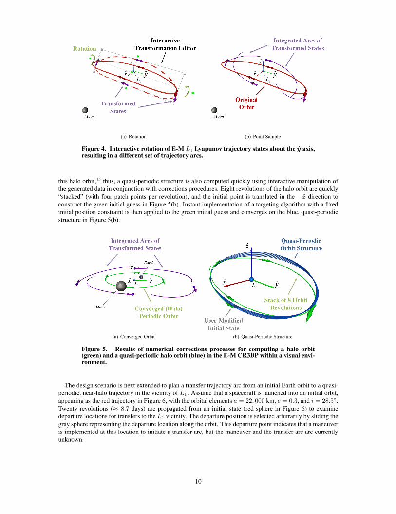
Since the extracted states are available to generate the visual scene, a spatial transformation is used toconstruct the initial guess for computing a periodic halo orbit. An interactive spatial transformation of thestates is achieved by using additional graphical elements that a user can manipulate inside the visual environ-ment. Thus, an initial guess for a halo orbit, as it appears in Figure 4(a), is produced by rotating the statescorresponding to the Lyapunov orbit counterclockwise about the mean y axis. The dashed line represents thetrace of the original orbit after an interactive rotation in the scene, and the purple points and vectors reflect thetransformed states. Clearly, the new states no longer produce a continuous trajectory when numerically prop-agated as demonstrated by the purple integrated arcs in Figure 4(b). However, the transformed states serveas a sufficient initial guess to generate the halo orbit. Thus, a user-created module for computing periodicorbits is applied to the transformed states. This computation tool for periodic orbits utilizes an asymmetric,variable-time multiple-shooting scheme.16 The resulting structure, appearing as the green orbit in Figure5(a), is a periodic halo orbit near the E-M L1 point. Quasi-periodic behavior exists in the close vicinity of

9

(a) Rotation (b) Point Sample

Figure 4. Interactive rotation of E-M L1 Lyapunov trajectory states about the y axis,resulting in a different set of trajectory arcs.

this halo orbit,15 thus, a quasi-periodic structure is also computed quickly using interactive manipulation ofthe generated data in conjunction with corrections procedures. Eight revolutions of the halo orbit are quickly“stacked” (with four patch points per revolution), and the initial point is translated in the −z direction toconstruct the green initial guess in Figure 5(b). Instant implementation of a targeting algorithm with a fixedinitial position constraint is then applied to the green initial guess and converges on the blue, quasi-periodicstructure in Figure 5(b).

(a) Converged Orbit (b) Quasi-Periodic Structure

Figure 5. Results of numerical corrections processes for computing a halo orbit(green) and a quasi-periodic halo orbit (blue) in the E-M CR3BP within a visual envi-ronment.

The design scenario is next extended to plan a transfer trajectory arc from an initial Earth orbit to a quasi-periodic, near-halo trajectory in the vicinity of L1. Assume that a spacecraft is launched into an initial orbit,appearing as the red trajectory in Figure 6, with the orbital elements a = 22, 000 km, e = 0.3, and i = 28.5◦.Twenty revolutions (≈ 8.7 days) are propagated from an initial state (red sphere in Figure 6) to examinedeparture locations for transfers to the L1 vicinity. The departure position is selected arbitrarily by sliding thegray sphere representing the departure location along the orbit. This departure point indicates that a maneuveris implemented at this location to initiate a transfer arc, but the maneuver and the transfer arc are currentlyunknown.

10

(a) Perspective View (b) Planar (xy) Projection

Figure 6. The initial Earth orbit for a mission to a quasi-periodic trajectory in thevicinity of L1 in the E-M system.

The transfer design process originates with a preliminary concept. An initial transfer option is constructedby incorporating orbital stability analysis, manifold propagation, and a maneuver testing tool. Stability infor-mation is obtained from the same periodic orbit generation tool that is employed to compute the halo orbitin Figure 5(a); the halo orbit in Figure 5(a) is unstable and possesses a stable and unstable subspace.16 Theinstability suggests that an asymptotic approach to the halo orbit, and the nearby quasi-periodic structure,exists. Therefore, the stable manifold approaching the halo orbit is determined using a computation modulethat is tailored with options for manifold generation such as the type of manifold (stable or unstable), thepropagation time, and the number of fixed points along the path. For this halo orbit, the computation modulepropagates the stable manifold for≈ 34.74 days employing 50 fixed points along the orbit. Subsequently, thestable manifold is added to the visualization (displayed in Figure 7). Unfortunately, there is no intersectionbetween the stable manifold that approaches the halo orbit and the initial orbit, indicating that an intermediatetransfer arc is required to bridge the gap.

(a) Perspective View (b) Planar (xy) Projection

Figure 7. Projection of the stable manifold (cyan) associated with a halo orbit (green)propagated in reverse time for 34.74 days.

The determination of an intermediate transfer is then achieved by testing potential maneuver vectors at anarbitrarily selected departure location on the initial orbit. At the gray departure location, some sample maneu-ver options are examined and displayed in Figure 8. A possible intermediate arc (black trajectory in Figure8(b)) intersects many manifold trajectories associated with the halo orbit. A manifold insertion location isthen visually selected where the intermediate transfer and the stable manifold trajectories intersect. Sinceseveral intersection locations are available, the intersection with the smallest change in the velocity directionbetween the intermediate transfer arc and the stable manifold trajectory is selected by visual inspection. Theintersection point (the purple sphere in Figure 9) is representative of a manifold insertion location and is,therefore, employed to isolate the portion of the intermediate transfer arc leading to stable manifold insertion

11

(a) (b)

Figure 8. Potential intermediate transfer arcs (black) explored through testing vari-ous maneuvers at the departure location (gray) on the initial orbit (red).

(roughly 3.5 revolutions of the transfer orbit). The final phase of the transfer is selected from the represen-tative collection of stable manifold trajectory arcs in Figure 9. The unused segment of the selected stablemanifold arc is snipped at the manifold insertion point. With the truncated intermediate and stable manifoldarcs, an initial guess for the transfer trajectory is accomplished.

(a) (b)

Figure 9. Views of an interactively constructed initial guess for a trajectory froman Earth orbit (red) to a quasi-periodic orbit (blue) in the vicinity of L1 in the E-Msystem.

An entire end-to-end trajectory is generated by implementing multiple shooting schemes with the inter-actively generated transfer guess. The proposed initial guess includes a departure maneuver from the initialorbit and a manifold insertion maneuver. The design is split into two shooting problems with a matching pointat the manifold trajectory insertion location: one problem computes adjustments to the intermediate transferarc (Transfer Leg 1), and the alternate problem addresses the asymptotic approach to a quasi-periodic orbitin the vicinity of L1 (Transfer Leg 2).

Since the manifold insertion point is not precisely on the stable manifold associated with the final quasi-periodic orbit, Transfer Leg 2 is computed first. The stable manifold arc is sampled to produce ten patchpoints using a direct sampling from the numerical propagation. Subsequently, the 32 patch points originallygenerated to compute the quasi-periodic orbit in Figure 5(b) are appended to the first ten patch points fromthe stable manifold arc to create an initial guess for Transfer Leg 2 (represented in Figure 10(a)). A multipleshooting computation module determines a continuous solution for the second transfer leg by employing avariable-time approach to enforce only continuity constraints. The resulting converged transfer, appearing asthe gold arc in Figure 10(a), flows freely into a quasi-periodic solution in the vicinity of L1. The resultingTransfer Leg 2 solution varies less in size than the initial guess (blue), but still achieves the objective. As

12

a result of the corrections procedure, the manifold insertion location shifts slightly to permit an asymptoticapproach.

The first transfer leg is then constructed following the determination of the asymptotic approach into thetarget orbit structure. The starting position that defines the converged Transfer Leg 2 (i.e., the manifoldinsertion location) is incorporated as a final position constraint for computing Transfer Leg 1. The initialguess for the first transfer leg (black) in Figure 9 is sampled and approximated as 29 states, including thedeparture location. The starting state corresponding to Transfer Leg 2 is then appended to these states to form30 patch points for the differential corrections process. Incorporation of a variable-time, multiple shootingalgorithm supplies the converged solution for the first transfer leg (Figure 10(b)) if the initial position is fixedat the departure maneuver and the final position is constrained to the manifold insertion location. As evidentin Figure 10(b), the converged Transfer Leg 1 possesses the same general shape as the initial guess with threephasing loops before the manifold insertion maneuver.

After the construction of both transfer legs, the visual analytics design approach renders the entire pathfrom the initial orbit to the L1 quasi-periodic orbit. Obviously, this design approach creates a visual repre-sentation of the complete trajectory inside a visual environment where the viewing angle is easily adjusted(Figure 10(c)). Also, the timing and maneuver details (summarized in Table 1) are obtained since that infor-

(a) Transfer Leg 2 (b) Transfer Leg 1

(c) End-to-End Trajectory

Figure 10. Visual analytics design scenario for a transfer trajectory from an Earthorbit (red) to the quasi-periodic orbit (gold) in the vicinity of L1 in the E-M system.

mation is available for computing continuous solutions with multiple shooting algorithms. The total transferfrom the departure maneuver to arrival at the quasi-periodic orbit is ≈ 19 days with a total ∆V equaling2.81765 km/s. This design is not necessarily fuel- or time-optimal, but it is constructed in one operation

13

using the visual analytics process for trajectory design. Additional constraints, such as timing or maneuvermagnitude bounds, can be easily incorporated. Since all the numerical data is available, subsequent analysisis facilitated. (Alternative multi-body design scenarios employing a visually-interactive process are availablein Reference 16.)

Table 1. Trajectory details for a transfer trajectory in Figure 10

Trajectory Event tStart (days) tEnd (days) ∆t (days) ‖∆V ‖ ( kms )

Starting Point 0 0 — —Initial Orbit 0 8.685 8.685 —Departure Maneuver (∆V1) 8.685 8.685 — 1.21834Transfer Leg 1 8.685 16.718 8.033 —Manifold Insertion (∆V2) 16.718 16.718 — 1.59931Transfer Leg 2 16.718 27.574 10.856 —Arrival 27.574 27.574 — —Quasi-Periodic Orbit 27.574 134.542 106.970 —

Total 0 134.542 134.542 2.81765

INTERACTIVE IMPLEMENTATION OF POINCARE SECTIONS

Poincare sections are a powerful tool for trajectory design within the context of multi-body models, but thecomputational cost is generally quite high due to the large volume of numerical integrations. In fact, interac-tive generation of a Poincare map in a series or even in a multi-core CPU parallel computational framework isnot always practical in real-time trajectory design. However, recent access to the parallel computing power ofgraphics processing units (GPUs) has created a new avenue for map generation. The construction of Poincaresections through general-purpose computation on GPUs and the corresponding interactive elements offermore immediate insight. Interactive capabilities permit a transient definition of any Poincare section that canpotentially unlock new options in multi-body regimes.

Interactively Defining a Poincare Section

A surface of section can be defined in terms of a vast set of hyperplanes, but the scope in this investigation islimited to one particular type. A Poincare map is defined by the returns of a trajectory to a specific hyperplane,Σ. If a real space is defined in terms of dimension N , E ∈ <N , any continuous hypersurface can define themapping for a section as long as the dimension of the hypersurface is less than N and the hypersurface istransversal to the flow.21 In the full CR3BP model, the equations of motion represent a six-dimensional (6D)space, so Σ can be defined as any hypersurface in 5D space (e.g., 1D curve, 2D surface, or a 3D object).Here, the hyperplane is restricted to a 2D plane in configuration space to permit interactive definition in avisual scene.

The hyperplane Σ is related to the rotating coordinate frame in the CR3BP through a rotation and a trans-lation. The frame R (x − y − z) is consistent with the rotating frame in the formulation of the CR3BP. Asecond coordinate frame, P , is then defined to be fixed on Σ with the origin at point O, and the directioncosine matrix RLP describes the orientation of P relative to R. A schematic in Figure 11 conveys the rela-tionship between the R and P frames. The normal to the plane Σ, i.e., n, identifies the first axis in the frameP . If point O is coincident with the barycenter B and P is initially aligned with R (such that RLP = I), theaxis n is parallel to the direction of x and the second axis in P , p, aligns with y. The unit vector q completesthe right-handed triad in the P frame. Also, the frame P may be translated relative to the barycenter B toincorporate planes in the rotating frame that do not intersect B. The vector T represents the translation of Σfrom the barycenter, B, to point O. When the translation vector T and the direction cosine matrix RLP = Iare defined, then Σ is constructed by applying the corresponding rotation and translation relative to the Rframe.

14

x

y

zT

Σ

O

B

p

q

n

Figure 11. A representation of the interactive hyperplane, Σ, as defined in a rotatingframe of reference.

User interaction defines the hyperplaneΣ through a graphical transformation in a visual environment. WithΣ represented by a graphical primitive, the transformation editor for shifting spatial data objects is employedto allow the user to interactively transform the rectangular polygon object. Therefore, the translation vector,T , and the rotation matrix, RLP , are defined through user interaction. The corners of the rectangular polygonare also scaled with the transformation editor, shaping Σ as either a rectangle or a square of an arbitrary size.These translation, rotation, and scaling operations are standard transformation elements in computer graphicsfor relating a local graphical object frame to a global coordinate frame.3 In this investigation, the graphicalobject is the rectangular polygon symbolizing Σ, as viewed in the rotating coordinate frame, defining P asthe local graphical object frame andR as the global coordinate frame. The interactively-defined planeΣ thenexists as input for a computation module that constructs Poincare sections.

The selection of initial conditions to seed a Poincare map is also based on the interactive definition of thehyperplane. After a user interactively transforms the graphical object representing a hyperplane, a structuredgrid of position coordinates that reside on the planar graphical object is outlined by the user. Each positioncoordinate in the grid possesses a distinct velocity magnitude for a user-specified Jacobi constant value.16 Aninitial state is then obtained by designating a velocity state that is parallel to the plane normal (n) with thedistinct velocity magnitude. Grids of initial states are implemented in a regular fashion with equal spacingbetween grid nodes.16 (A detailed mathematically description is available in Reference 16.)

GPU Computation for Poincare Sections

The capability for parallel computation that is available with graphics processing hardware (GPU) enablesthe implementation of Poincare mapping techniques during a visual design process. Recall that visual analyt-ics components require real-time computational speeds (i.e., up to a few seconds) for an interactive discoveryprocess.12 Unfortunately, most Poincare map calculations imply a struggle to meet real-time speeds due tothe number and density of the numerical integrations that are necessary to observe the behavior of the localflow. The computation of a Poincare section on a computer processor (CPU) is quite sluggish if the numericalsimulation is implemented sequentially. However, parallel processing applications are ideal for generatingPoincare maps since each numerical integration involved in the generation of a section is independent. For-tunately, GPUs are designed for intensive, highly-parallel computations–a necessity for graphics renderingapplications (e.g., color blending and shading operations). With recent interest in expanding parallel comput-ing beyond the realm of gaming graphics, GPU manufacturers such as NVIDIA are releasing programminginterfaces that can supply significant support for engineering problems. The parallel computational power ofthe GPU introduces a Poincare map as a real-time, visual trajectory design methodology.

Numerical simulation and detection of Σ plane crossings are achieved by simple algorithms for a smoothintegration with CUDATM – a GPU programming language developed by NVIDIA. A Runge-Kutta 4th-ordernumerical integration scheme (RK4) is employed since the implementation involves straightforward, linear

15

computations that enhance the computational efficiency with CUDATM.16 The Poincare map approximatesreturns to the plane Σ via linear interpolation between numerical integration steps since the step size for anRK4 scheme must be fairly small (h < 1× 10−5) to describe the motion in the CR3BP. For added versatility,the user may select to generate the map with either (i) single precision for greater computational speed, or(ii) double precision for enhanced accuracy.

A Sample Near-Earth Hyperplane in the Earth-Moon System

A simple Poincare map is employed to illustrate the interactive capabilities with visual analysis in theCR3BP. Since the map generation techniques explore high-dimensional behavior by design, the hyperplaneΣ1 is selected to compute some planar initial conditions in conjunction with out-of-plane trajectories forcomparison in the E-M system. Through user interaction, the plane Σ1 is positioned in the xz plane near theEarth on the +x side with the plane normal n directed opposite to y, (i.e., Σ1 : −y = 0). In Figure 12(a),a green square represents Σ1 with one edge intersecting the x axis. An 8 × 8 grid (i.e., 64 initial states)seeds the Poincare map and is also displayed in Figure 12(a) as colored arrows that are scaled by velocitymagnitude. Again, the Jacobi constant value, pre-specified as C = 3.12 in this initial simulation, determinesthe velocity magnitude at each initial position. Each initial state on Σ1 is assigned an unique color basedon an index number and a rainbow colormap. The purple and dark blue initial states, therefore, representplanar initial conditions for the map, and all other initial condition vectors possess a positive z componentin position. Also, preliminary intuition concerning the behavior is available through a rendering of the zero-velocity surface corresponding to this value of Jacobi constant. Viewed as a white surface in Figure 12(a),this C value allows a wide range of motion including escape through the libration point gateways, implyinga possible chaotic response.

Once the plane Σ1 is placed appropriately through user interaction, a Poincare map is computed withthe GPU and examined within the visual environment. A user determines the number of returns and thesimulation length. For this example, the two-sided Poincare map for the 8× 8 grid of initial states in Figure12(a) is computed with a GPU simulation in under a few seconds, meeting the real-time computation speedsrequired by visual analytics. Up to 100 returns to the plane Σ1, over a time span of 434 days, are capturedwith the GPU parallel computational processes; the results are subsequently visualized in configuration space(Figure 12(b)). A positive or negative crossing is easy to distinguish in Figure 12(b) since the positive returns(y < 0) reside on the same side of the Earth as Σ1. As is apparent in Figure 12(b), none of these initialstates generate trajectories that leave Earth-vicinity, even though the L1 and L2 gateways are open. Visually

n

p

qZero-Velocity

Surface

1 Moon

2L1L

4L

xy

z

Earth

Initial

Conditions

(a) Initial Conditions

n

p

q

xy

z

Zero-Velocity

Surface

1 Moon

2L1L

Earth

(b) Two-sided Poincare Map

Initial Condition Number

0 63

Figure 12. The hyperplane Σ1 and the associated Poincare map for an 8 × 8 gridof initial states simulated for 434 days with up to 100 returns per initial state in E-Msystem (C = 3.12).

16

interesting trajectories are selected for analysis in configuration space using pick-callbacks within the scene.A user-selected point with a mouse click returns an index that is then back-traced to the corresponding initialstate. The same initial condition is, in turn, simulated again but visualized as an entire trajectory over time.A planar (xy) trajectory (purple curve in Figure 13(a)) demonstrates typical in-plane quasi-periodic behavior(i.e., the trajectory precesses about a primary in the rotating view but is not periodic). A second trajectorythat originates with a small out-of-plane component is also selected for comparison (light blue trajectoryin Figure 13(b)). The out-of-plane trajectory possesses quasi-periodic behavior that is quite similar to thein-plane quasi-periodic orbit, but the initial out-of-plane component tends to shape trajectories into a 3D“bowl” structure in configuration space as evident from two out-of-plane trajectories selected for observationin Figures 13(c) and 13(d). The generation of these trajectories from the Poincare section representationallows a user to implement Poincare maps as part of the visual analytics design process.

n

p

q

1

x

y

z

Earth

(a) Planar (xy) Trajectory

n

p

q

x

y

z

1

Earth

(b) Trajectory with a Small z Component

n

p

q

x

y

z

1

Earth

(c) Out-of-Plane Trajectory

n

p

q

x

y

z

1

Earth

(d) Out-of-Plane Trajectory

Initial Condition Number

0 63

Figure 13. Trajectories selected from the Poincare section in Figure 12(b) (C = 3.12in the E-M system).

A Sample Hyperplane Near L5 in the Earth-Moon System

Another sample hyperplane in the Earth-Moon system is the basis for a map that resides in the vicinityof the L5 libration point. For this example, the hyperplane Σ2 is interactively translated to intersect L5 andoriented such that n = x. Shaped as a rectangle in this example with the long dimension in the p direction,the blue hyperplane in Figure 14(a) is defined as Σ2 : x = 0.487512. The Jacobi constant value is pre-specified as C = 2.96, which pulls the zero-velocity surface completely out of the xy plane. Therefore, allthe initial states that are defined on an 8×8 grid on the planeΣ2, also apparent in Figure 14(a), exist in a validregion of flow. A quick GPU simulation generates a two-sided Poincare map that evaluates up to 100 returnsper initial state over 434 days. Visualizing the returns in configuration space as uniformly scaled spheres with

17

a unique color for each initial state (Figure 14(b)), the trajectories appear to traverse a vast range of space;returns are located far beyond L4 and L5 in the ±y directions yet expand across a wide array of z values.

The visualization is modified to display additional information from the map such that orbital structuresin the vicinity of the L5 libration point are located. To gather insight concerning the returns, the sphereobjects representing the returns to the map are scaled based on the crossing number, cn, which defines theaccumulated number of returns. With this cn scaling, smaller spheres correspond to the first few crossingsof the hyperplane Σ2, whereas, larger spheres imply a crossing preceded by many previous returns. Theresulting visualization, displayed in Figure 14(c), highlights two groups or clusters of orange and greencrossings. Each group of crossings possesses the same color (i.e., originates from the same initial condition)and collects spheres of various sizes in the same general locations. Employing user selection for the greenset of clusters reveals an out-of-plane orbit structure near L5 that exhibits behavior similar to a quasi-periodicorbit for the specified time interval (Figure 14(c)). However, the green trajectory is not truly quasi-periodicsince this orbital structure is not explicitly seeded inside the center subspace corresponding to a nearbyperiodic orbit.15 However, the green trajectory does remain in the vicinity of L5 for the simulation length(≈ 434 days) and may remain in this vicinity longer with station keeping. With a visual analytics trajectorydesign approach, though, trajectories selected from a Poincare section are immediately available and canbe implemented as the focus of further analysis. (Reference 16 conveys additional sample hyperplanes andsection visualization options.)

n

p

qZero-Velocity

Surface 2

Initial

Conditions

xy

z

5L

(a) Initial Conditions

np

q

Moon

4L

1L

xy

z

5L

3L

2

(b) Returns with Uniformly Sized Spheres

np

q

xy

z2

4L

5L

3L

Cluster

Groups

(c) Scaled Returns and Selected Arc

n

p

Earth 2Lx

y

5L

3L 1L

Moon

(d) Planar (xy) Projection

Initial Condition Number

0 63

Figure 14. The two-sided Poincare map for the hyperplane Σ2 that intersects L5 inthe E-M system (C = 2.96).

18

SUMMARY AND CONCLUSIONS

The application of visual analytics to trajectory development demonstrates the interactive capabilities andthe rapid design capabilities that are accessible in a visual environment. Interactive tools can also enhance au-tomated design processes. Trajectory design within a visual scene or graphical user interface (GUI) expeditesthe design process when compared to segregated operations such as the manual manipulation of data and tar-geting schemes operated outside of a visualization component. When the governing differential equations arenot solvable analytically, these capabilities can be an enabling technology. Expanding these functionalitiesinto other design applications offers opportunities for rapid trajectory development and information discoverywith various dynamical models – all via a visual environment.

A comprehensive interface for designing spacecraft trajectories that applies the various facets of the visualanalytics process is introduced. Designs can originate with just small amounts of information, and all sub-sequent steps can be implemented visually in real-time to plan entire end-to-end trajectories. Unique userinsight is also incorporated. Every step towards a design objective occurs in a single sitting through user-interactions with visualizations, data structures, and targeting algorithms. In the application to the CR3BP,the visual analytics design strategy requires a user with more experience in dynamical systems, but the resultsare generated exceptionally fast with a significantly reduced level of manual input.

The implementation of Poincare maps in a real-time design setting is also explored for multi-body scenar-ios. The parallel computational power of the GPU is exploited to generate Poincare sections for 2D grids ofinitial states in seconds, yielding map results that are available for almost instant analysis. Interactive trans-formation editors allow a hyperplane to be defined at any orientation and location; although the exampleshave all employed hyperplanes in configuration space, the concept is not limited to physical space. Interpre-tation of the information available in a map is aided by exploiting graphical options such as scale and colorand by incorporating pick-callbacks to instantly view trajectories from the map.

With this application of visual analytics, extensions to this are available for further investigation. Oneelement that greatly increases the appeal of trajectory design with visual analytics is an interactive and adap-tive process for applying constraints on trajectory arcs. Expanding the applications of Poincare maps andsurfaces of section is also a priority. The results in this investigation display a real-time implementation ofPoincare sections, but there are many more functionalities to be explored. An extension to higher-fidelitymodels, e.g., time-varying and ephemeris models, is a continuing effort which, in turn, requires explorationof higher-fidelity numerical propagation on GPU architectures.

ACKNOWLEDGMENT

The authors are extremely grateful to Rune and Barbara Eliasen for their support of this research and fund-ing for the Rune and Barbara Eliasen Visualization Laboratory at Purdue University. Also, the authors wishto acknowledge Visualization Sciences Group (the developers of Avizo R© ) for programming and implemen-tation assistance with the interactive and visualization tools in this work. This effort is also supported by theCollege of Engineering and the School of Aeronautics and Astronautics at Purdue University.

REFERENCES

[1] J. Carrico and E. Fletcher, “Software Architecture and Use of Satellite Tool Kit’s Astrogator Modulefor Libration Point Orbit Missions,” Libration Point Orbits and Applications, Parador d’Aiguablava,Girona, Spain, June 2002.

[2] A. Keim, F. Mansmann, J. Schneidewind, J. Thomas, and H. Ziegler, “Visual Analytics: Scope andChallenges,” Visual Data Mining, LNCS 4404 (S. Simoff, M. Bohlen, and A. Mazeika, eds.), pp. 76–90,Springer-Verlag, Berlin, 2008.

[3] A. Watt, 3D Computer Graphics. Pearson, Addison-Wesley, Harlow, England, 2000.[4] M. W. Lo, R. L. Anderson, G. Whiffen, and L. Romans, “The Role of Invariant Manifolds in Low Thrust

Trajectory Design (Part I),” AAS/AIAA Spaceflight Dynamics Conference, Maui, Hawaii, February 2004.Paper AAS 04-288.

19

[5] R. L. Anderson and M. W. Lo, “The Role of Invariant Manifolds in Low Thrust Trajectory Design (PartII),” AAS/AIAA Specialist Conference, Providence, Rhode Island, August 2004. Paper AIAA 2004-5305.

[6] M. W. Lo, R. L. Anderson, T. Lam, and G. Whiffen, “The Role of Invariant Manifolds in Low ThrustTrajectory Design (Part III),” AAS/AIAA Spaceflight Dynamics Conference, Tampa, Florida, January2006. Paper AAS 06-190.

[7] W. S. Koon, M. W. Lo, J. E. Marsden, and S. D. Ross, “Heteroclinic Connections between PeriodicOrbits and Resonance Transistions in Celestial Mechanics,” Chaos, Vol. 10, No. 2, 2000, pp. 427–469.

[8] M. Vaquero and K. C. Howell, “Poincare Maps and Resonant Orbits in the Circular Restricted Three-Body Problem,” AAS/AIAA Astrodynamics Specialist Conference, Girdwood, Alaska, August 2011. Pa-per AAS 11-428.

[9] K. Museth, A. Barr, and M. W. Lo, “Semi-Immersive Space Mission Design and Visualization: CaseStudy of the Terrestrial Planet Finder Mission,” IEEE Visualization Conference Proceedings, 2001.

[10] J. Thomas and K. Cook, Illuminating the Path: Research and Development Agenda for Visual Analytics.IEEE Press, Los Alamitos, 2005.

[11] J. Risch, A. Kao, S. R. Poteet, and Y.-J. J. Wu, “Text Visualization for Visual Text Analytics,” VisualData Mining, LNCS 4404 (S. Simoff, M. Bohlen, and A. Mazeika, eds.), pp. 154–171, Springer-Verlag,Berlin, 2008.

[12] M. L. Huang and Q. V. Nguyen, “Context Visualization for Visual Data Mining,” Visual Data Mining,LNCS 4404 (S. Simoff, M. Bohlen, and A. Mazeika, eds.), pp. 248–263, Springer-Verlag, Berlin, 2008.

[13] D. Stalling, M. Westerhoff, and H.-C. Hege, “Amira: A Highly Interactive System for Visual DataAnalysis,” The Visualization Handbook (C. D. Hansen and C. R. Johnson, eds.), pp. 749–767, ElsevierAcademic Press, Boston, Massachusetts, 2005.

[14] E. J. Doedel, V. A. Romanov, R. C. Paffenroth, H. B. Keller, D. J. Dichmann, J. Galan-Vioque, andA. Vanderbauwhede, “Elemental Periodic Orbits Associated with the Libration Points in the CircularRestricted 3-Body Problem,” International Journal of Bifurcation and Chaos, Vol. 17, No. 8, 2007,pp. 2625–2677.

[15] G. Gomez, W. S. Koon, M. W. Lo, J. E. Marsden, J. Masdemont, and S. D. Ross, “Connecting orbits andinvariant manifolds in the spatial restricted three-body problem,” Nonlinearity, Vol. 17, 2004, pp. 1571–1606.

[16] W. Schlei, “An Application of Visual Analytics to Spacecraft Trajectory Design,” M.S. Thesis, Schoolof Aeronautics and Astronautics, Purdue University, West Lafayette, Indiana, 2011.

[17] W. H. Press, S. A. Teukolsky, W. T. Vetterling, and B. P. Flannery, Numerical Recipes: The Art ofScientific Computing. Cambridge University Press, New York, 3rd ed., 2007.

[18] H. B. Keller, Numerical Methods for Two-Point Boundary-Value Problems. Ginn-Blaisdell Pub. Co.,Waltham, Massachusetts, 1968.

[19] J. Stoer and R. Bulirsch, Introduction to Numerical Analysis. Springer, Berlin, 3rd ed., 2002.[20] E. Canalias and J. J. Masdemont, “Computing natural transfers between Sun-Earth and Earth-Moon

Lissajous libration point orbits,” Acta Astronautica, Vol. 63, No. 1-4, 2008, pp. 238–248.[21] L. Perko, Differential Equations and Dynamical Systems. Springer, New York, 3rd ed., 2001.

20