ab initio based multi-scale simulations of oxide .../ab initio based multi... · ab initio based...

KUNGLIGA TEKNISKA HOGSKOLAN

PHELMA

Master in Energy and Nuclear Engineering

Reactor Physics Department

Master Thesis

Ab Initio based Multi-Scale

Simulations of Oxide Dispersion

Strengthened Steels

Antoine Claisse

Supervisors:

Dr. Par Olsson

Dr. David Rodney

Academic year 2011-2012

“All you create, all you destroy,

All that you do, all that you say [...]

And everything under the sun is in tune

But the sun is eclipsed by the moon.

Pink Floyd, 1973

V

Abstract

The growing need to produce clean energy requires the development of

new nuclear plants using less fissile materials. These plants operate at high

temperatures and yield high neutron fluxes. The current structural materials

can not withstand these conditions and a new class of steels is therefore un-

der development. These steels must be resistant to swelling, ductile to brittle

transition temperature shift and creep induced by irradiation. The Oxide

Dispersion Strengthened (ODS) steels seem to be a good answer to these

requirements and the experiments confirm that their mechanical properties

are much better than for classic austenitic and ferritic-martensitic steels.

However, their performances are due to the high density of oxide nanoclus-

ters in the material, which trap helium before it forms bubbles and prevent

the dislocations from moving, and these clusters are not well understood

yet.

An ab-initio study has been performed on Cr, Y, Ti and O in an iron

lattice using the Density Functional Theory (DFT). The stable position of

each of these solutes in the iron matrix has firstly been determined. Then,

all the pair interactions of the solutes between each other and with a va-

cancy have been calculated up to the fifth nearest neighbour, as well as the

migration energy of these solutes. The goal of these simulations was to ob-

tain enough data to understand the formation process of (Y,Ti,O) clusters

in an iron lattice. Special considerations have been given to the interactions

between a vacancy and an yttrium atom and a vacancy and oxygen atoms,

in both cases because of the very strong attraction between them. The sec-

ond part of this work is based on Atomistic Kinetic Monte Carlo (AKMC)

simulations of systems using the data acquired from the first-principles cal-

culations. Due to calculating power constraints, several approximations had

to be done for the migration energies of Y and O. This caused a difficulty

in converting the AKMC code time into a real time. Additional simulations

were run to try to establish the stability range of the clusters. The results

show that (Y,Ti,O) clusters can be formed at 1200 K thanks to the vacancy

assisted diffusion mechanism. They are reasonably stable at 600 K without

vacancy, but a vacancy helps achieving a higher stability. A vacancy can

also trap up to 6 oxygens.

VI

Sammanfattning

Det vaxande behovet att producera ren energi kraver utveckligen av nya

karnkraftverk som anvander mindre klyvbara amnen. Dessa verkar vid hoga

temperaturer och skapar hoga neutronfloden. De nuvarande strukturella

materialen tal inte dessa villkor och en ny klass av stal ar darfor under

utveckling. Dessa stal maste tala svullnad, omslagstemperaturforskjutning

och kryppning, alla av dessa under bestralning. Oxidforstarkta stal (ODS)

ser ut som ett bra svar for dessa behov och erfarenheter bekraftar att deras

mekaniska egenskaper ar mycket battre an for de traditionella austenistika

och ferristisk-martensistika stalen. Deras prestationformaga beror pa den

hoga densiteten av oxidkluster i materialet som fangar helium innan de ska-

par bubblor, och forhindrar dislokationernas forflyttning, och dessa kluster

a inte an forstadda.

En ab initio analys genomfordes med Cr, Y, Ti och O i en jarnmatris

med hjalp av tathetsfunktionalteorin (DFT). Varje elements stabila posi-

tion i jarnmatrisen utrondes forst. Darefter beraknades alla parvaxelverkan

mellan dessa atomer och mellan dem och en vakans upp till den femte

narmaste grannen. Migrationenergin beraknades ocksa. Malet med dessa

simuleringar ar att skaffa tillrackligt med data for att forsta formation-

processen av (Y,Ti,O) kluster i en jarnmatris. Sarskild hansyn gavs till

vaxelverkan mellan en vakans och en yttriumatom och mellan en vakans och

syreatomer, eftersom det finns en mycket stark vaxelverkan mellan dem tva i

bada fallen. Den andra delen av detta arbete grundas pa atomistisk kinetisk

Monte Carlo (AKMC) simulationer som anvander ab initio data fran den

forsta delen. Pa grund av berakningskraftbegransningar gjordes nagra ap-

proximationer pamigrationenergin av Y och O. Detta medforde en svarighet

for att konvertera AKMC tiden till verklig tid. Fler simulationer utfordes

for att forsoka att etablera stabilitetsomradet for dessa kluster. Resultatet

ar att (Y,Ti,O) kluster kan skapas vid 1200 K tack vare den vakansdrivna

diffusionmekanismen. De ar rimligt stabila vid 600 K utan vakanser, men

en vakans hjalper att na en hogre stabilitet. En vakans kan ocksa fanga up

till sex syreatomer.

VII

Resume

La demande croissante en energie propre exige le developpement de nou-

velles centrales nucleaires utilisant moins de materiaux fissiles. Ces centrales

fonctionnent a temperature elevee et produisent d’importants flux de neu-

trons. Les materiaux de structure actuels ne sont pas capables de supporter

ces conditions, et un nouveau type d’aciers est donc en developpement. Ces

aciers doivent etre resistants au gonflement, au decalage de la temperature

de transition ductile-fragile et au fluage, le tout sous irradiation. Les aciers

durcis par dispersion d’oxydes (ODS) semblent bien repondre a ces deman-

des et les experiences confirment que leurs proprietes mecaniques sont bien

meilleures que celles des aciers classiques tels que les austenitiques et les

ferritiques-martensitiques. Cependant, leurs performances sont dues a la

haute densite de nano-amas d’oxydes dans le materiau qui piegent les atomes

d’helium avant qu’ils ne puissent former des bulles et empechent les dislo-

cations de bouger. Ces amas ne sont pas encore bien compris.

Une etude ab initio sur le chrome, l’yttrium, le titane et l’oxygene dans

un cristal de fer a ete effectuee en utilisant la theorie de la fonctionnelle de

la densite (DFT). La position d’equilibre de ces atomes en solution solide

dans un cristal de fer a ete determinee dans un premier temps. Ensuite,

toutes les interactions de paire entre ces atomes et entre ces atomes et une

lacune ont ete calculees jusqu’au 5eme plus proche voisin. Les energies de

migration de ces elements ont egalement ete calculees. Le but de ces sim-

ulations etait d’obtenir des informations sur le processus de formation des

amas de (Y,Ti,O) dans un cristal de fer. Une attention particuliere a ete

apportee aux interactions entre une lacune et un atome d’yttrium et entre

une lacune et des atomes d’oxygene, dans les deux cas a cause de l’attraction

tres forte entre eux. La seconde partie de ce travail est basee sur des simula-

tions Monte Carlo cinetiques atomistiques (AKMC) de systemes en utilisant

les donnees issues des simulations ab initio. A cause de limitations sur la

puissance de calcul disponible, plusieurs approximations ont du etre faites

concernant les energies de migration de Y et O. Cela a cause des difficultes

dans la conversion du temps Monte Carlo en temps reel. Des simulations

additionnelles ont ete faites pour essayer de trouver le domaine de stabilite

des amas. Les resultats montrent que les amas de (Y,Ti,O) peuvent etre

formes a 1200 K grace au mecanisme de diffusion assistee par lacune. Ils

sont raisonnablement stables a 600 K sans lacune, mais une lacune aide a

atteindre une plus grande stabilite. Une lacune peut aussi pieger jusqu’a 6

atomes d’oxygene.

VIII

Acknowledgements

I wish to use this page to thank many people, some of them I never had

the occasion to do it viva voce. A lot of people have helped me becoming

who I am today, both on a professional and on a personal level, and I start

with a general thank you.

Three years ago, I found myself hesitating between different fields of

physics. I was not able to make a decision, and therefore was multiplying

the introductory classes. That is when I met Roger Brissot. His passion

about nuclear science was remarkable. He has this unique ability to make

the students want to know more all the time. He is the reason I chose nuclear

sciences over other exciting topics. Three years after, I am really enjoying

what I am doing, so to him, I address a special thank.

Another teacher who inspired me more than he thinks is David Rodney.

He taught me my first notions of numerical analysis and gave me the oppor-

tunity to work one summer with one of his former co-worker in the research

field. We had a really inspiring talk about research and especially simula-

tions and, if I remember turning him down when he offered me a PhD, I am

now convinced that this is what I want to do. I hope to have the occasion

to work with you one day, and I am already grateful for all you did for me.

I enjoyed very much doing my master thesis at KTH, in the Reaktorfysik

department. Everyone there was friendly with me, and helped me when I

needed help. I’d like to thank Par Olsson, for his help, his patience and his

availability. He has many times given me advices and always answered my

questions with a great precision and kindness. He trusted me to carry on

this research and pushed me to give the best at all time. I have learnt a lot

from him and am really thankful.

I also wish to thank my friends and my family, who have always been

there for me. Thank you Fabio, Milan, Sarah, Zhonweng and everyone who

contributed to make the working environment and the lunchtimes so pleas-

ant. Many thanks to my Erasmus friends; Clara, Tobias, Victor, Nacho and

of course Sibel, for dinners, apple cakes, sport, games, and about everything

not work-related for the last 18 months. Merci maman et papa for always

supporting me in my choices and thank you Justine for proving me that

friendship is stronger than distance, and of course the careful proofreading

of this thesis.

I acknowledge financial support from the European Fusion Development

Agreement (EFDA). Most of the computer simulations have been performed

on the resources provided by the Swedish National Infrastructure for Com-

puting (SNIC) at PDC.

Abbreviations and

nomenclature

0.0.0.1 List of abbreviations

1-5NN - First-Fifth Nearest Neighbour

ACRDF - Averaged Compared Radial Distribution Function

AKMC - Atomistic Kinetic Monte Carlo

BCC - Body-centered cubic (cell)

DBTT - Ductile-brittle transition temperature

dpa - Displacements per atom

DFT - Density Functional Theory

FCC - Face-centered cubic (cell)

FIA - Foreign Interstitial Atom

Gen-IV - Generation IV

HEG - Homogeneous Electron Gas

HF - Hartree-Fock

HK - Hohenberg Kohn

GGA - Generalized Gradient Approximation

KTH - Kungliga Tekniska Hogskolan

LAKIMOCA - LAttice KInetic MOnte CArlo

LDA - Local Density Approximation

MC - Monte Carlo

MD - Molecular Dynamic

MEP - Minimum Energy Path

NEB - Nudged Elastic Band

ODS - Oxide Dispersion Strengthened

PAW - Projector Augmented Wave

PBE - Perdew Burke Ernzerhof

SIA - Self Interstitial Atom

VASP - Vienna Ab-initio Simulation Package

X

0.0.0.2 Element symbols

C - Carbon

Cr - Copper

Fe - Iron

He - Helium

Mo - Molybdenum

Mn - Manganese

Nb - Niobium

Ni - Nickel

O - Oxygen

P - Phosphorus

S - Sulfur

Si - Silicon

Ti - Titanium

V - Vacancy (not Vanadium in this work)

W - Tungsten

Y - Yttrium

Zr - Zirconium

0.0.0.3 Physical quantities

kB - Boltzmann’s constant

Contents

Abstract V

Sammanfattning VI

Resume VII

Acknowledgements VIII

Nomenclature IX

List of Figures XIII

List of Tables XIV

1 Introduction/Motivations 1

1.1 Background . . . . . . . . . . . . . . . . . . . . . . . . . . . . 1

1.2 Aims of the work . . . . . . . . . . . . . . . . . . . . . . . . . 3

2 Theoretical background 5

2.1 Density Functional Theory . . . . . . . . . . . . . . . . . . . 5

2.1.1 Hamiltonian . . . . . . . . . . . . . . . . . . . . . . . . 6

2.1.2 Wavefunctions . . . . . . . . . . . . . . . . . . . . . . 11

2.1.3 Vienna Ab-initio Simulation Package . . . . . . . . . . 14

2.2 Kinetic Monte Carlo . . . . . . . . . . . . . . . . . . . . . . . 15

2.2.1 Atomic Kinetic Monte Carlo . . . . . . . . . . . . . . 18

2.2.2 LAttice KInetic MOnte CArlo . . . . . . . . . . . . . 19

2.3 Materials irradiation . . . . . . . . . . . . . . . . . . . . . . . 20

2.3.1 Defects . . . . . . . . . . . . . . . . . . . . . . . . . . 20

2.3.2 Energies . . . . . . . . . . . . . . . . . . . . . . . . . . 21

2.3.3 Macroscopic effect of irradiation . . . . . . . . . . . . 22

2.3.4 Oxide Dispersion Strengthened (ODS) steels . . . . . 25

XII CONTENTS

3 Results 27

3.1 Ab-initio calculations . . . . . . . . . . . . . . . . . . . . . . . 27

3.1.1 stable position of solutes . . . . . . . . . . . . . . . . . 28

3.1.2 Interactions with vacancies . . . . . . . . . . . . . . . 31

3.1.3 Migration of the solutes . . . . . . . . . . . . . . . . . 37

3.1.4 Interactions between solutes . . . . . . . . . . . . . . . 40

3.1.5 Clustering . . . . . . . . . . . . . . . . . . . . . . . . . 43

3.2 Atomic kinetic Monte-Carlo . . . . . . . . . . . . . . . . . . . 46

3.2.1 Approximations and modifications . . . . . . . . . . . 46

3.2.2 Formation of clusters . . . . . . . . . . . . . . . . . . . 49

3.2.3 Stability of clusters under normal conditions . . . . . 55

4 Conclusions 57

List of Figures

2.1 Flow-chart of a typical DFT calculation within the Kohn-

Sham framework. . . . . . . . . . . . . . . . . . . . . . . . . . 9

2.2 Illustration of the pseudopotential and of the pseudo wave-

function. . . . . . . . . . . . . . . . . . . . . . . . . . . . . . . 12

2.3 Illustration of the images in the NEB method . . . . . . . . . 16

2.4 Map of the simulation methods depending on the aimed timescale

and lengthscale. . . . . . . . . . . . . . . . . . . . . . . . . . . 17

2.5 Different types of defects in a crystal . . . . . . . . . . . . . . 20

2.6 Influence of the chromium content on the DBTT shift. . . . . 24

3.1 Tensile, compressed and mixed sites. . . . . . . . . . . . . . . 28

3.2 5 nearest octahedral position from a regular lattice site . . . . 32

3.3 Illustration of a couple V-O moving. . . . . . . . . . . . . . . 34

3.4 Geometry of vacancy-oxygen clusters. . . . . . . . . . . . . . 35

3.5 Relaxation of the oxygen atoms around a vacancy. . . . . . . 36

3.6 Differential electron density for 1 and 6 octahedral O around

a vacancy. . . . . . . . . . . . . . . . . . . . . . . . . . . . . . 37

3.7 Illustration of the Y-V relaxation. . . . . . . . . . . . . . . . 39

3.8 Position of the Y atom when first nearest neighbour of a va-

cancy for a temperature oscillating around 2000 K. . . . . . . 39

3.9 Illustration of the vacancy diffusion mechanism. . . . . . . . . 40

3.10 The eleventh nearest octahedral neighbours of an octahedral

site. . . . . . . . . . . . . . . . . . . . . . . . . . . . . . . . . 43

3.11 Binding energy of O with it’s eleventh first nearest neighbours

O. . . . . . . . . . . . . . . . . . . . . . . . . . . . . . . . . . 44

3.12 Most stable configurations for Y2TiO3. . . . . . . . . . . . . . 45

3.13 System Cr-Ti at 1200 K after 2.9 seconds. . . . . . . . . . . . 51

3.14 System Cr-Y at 1200 K after 98 days. . . . . . . . . . . . . . 51

3.15 System Cr-Ti-Y at 1200 K after 90 days. . . . . . . . . . . . . 52

3.16 System Cr-Ti-O at 1200 K after 37 µs. . . . . . . . . . . . . . 53

XIV LIST OF FIGURES

3.17 System Cr-Y-O at 1200 K after 127 µs. . . . . . . . . . . . . 53

3.18 System Cr-Ti-Y-O at 1200 K after 153 µs. . . . . . . . . . . . 54

3.19 Clusters at 1200 K after 153 µs. . . . . . . . . . . . . . . . . . 54

List of Tables

2.1 Value of π given by a MC process depending on the number

of events . . . . . . . . . . . . . . . . . . . . . . . . . . . . . . 17

2.2 Composition of some steels in weight %. . . . . . . . . . . . . 23

3.1 Solution energies (eV) . . . . . . . . . . . . . . . . . . . . . . 30

3.2 Binding energies (eV) SIA-solute . . . . . . . . . . . . . . . . 31

3.3 Distance between the nearest neighbours (in unit of lattice

parameter . . . . . . . . . . . . . . . . . . . . . . . . . . . . . 31

3.4 Binding energies with a vacancy. . . . . . . . . . . . . . . . . 33

3.5 Binding and relative binding energies of oxygens with a vacancy. 36

3.6 Migration energies of solutes in an iron BCC lattice. . . . . . 37

3.7 Binding energies of solutes with Cr. . . . . . . . . . . . . . . 41

3.8 Binding energies of solutes with Ti. . . . . . . . . . . . . . . . 42

3.9 Binding energies of solutes with Y. . . . . . . . . . . . . . . . 42

3.10 Value of the time conversion coefficient. . . . . . . . . . . . . 50

XVI LIST OF TABLES

Chapter 1

Introduction/Motivations

1.1 Background

In the global effort to reduce the emissions of greenhouse gases, the coal and

gas plants have to be limited in favor of clean energies, such as renewable

and nuclear energies. However, the uranium reserves are limited and current

reactors will run out of fuel in the next decades or centuries. It is then

necessary to develop new technologies to overcome this issue; the fourth

generation of breeder reactors or, in a hypothetical future, the fusion reactors

will drastically reduce the need for rare materials for the fuel. In addition to

that, they will produce much less nuclear wastes, and the fission reactors can

even burn some with an appropriate design. These new technologies operate

at high temperatures, in non chemically inert environments and produce

high neutron radiation fields. These peculiar conditions, and especially the

irradiation, lead to a need in a new class of materials able to withstand such

an environment. For the structural materials usually made of steels, this

means that they need to be made more radiation resistant. A tremendous

effort is made in investigating several kinds of steels with different phases

for the iron lattice as well as different compositions, in order to find those

which are most likely to be a solution.

Previous studies have already shown that the three main issues with

structural steels are swelling, embrittlement, and thermal creep. These

problems can weaken the answer to transient and lower the resistance to fa-

tigue. Concerning swelling, austenitic steels (with a face-centered cubic (fcc)

structure) can in the best case resist 120 displacements per atom on average

(dpa), due to the production of helium. This case is reached if titanium is

present in the steel. However, to keep the crystal structure, nickel is present

to act as a stabilizer and has a high (n,α) cross section. Ferritic-martensitic

2 1. Introduction/Motivations

steels (with a body-centered cubic (bcc) structure), without nickel, can resist

around 200 dpa, which would correspond to around five years in a fast neu-

trons reactor. The ductile to brittle transition temperature shift is mainly

a problem at low temperature, when irradiation yields a larger shift. The

shift can reach up to 250 degrees depending on the conditions and is lower in

presence of chromium. The thermal creep is mostly an issue for irradiation

at high temperature and for this problem as well as for the embrittlement,

austenitic steels are better than the ferritic-martensitic ones.

However, as good as these steels are, they all have drawbacks and it is

necessary to develop a new technology which would have both a high creep

strength, to allow operating at higher temperatures than the displacement

damage regime limit, and be resistant to swelling, trapping the He atoms

before they do any damage, forming bubbles. One of the most promising way

to fulfill these requirements is to use oxide dispersion strengthened (ODS)

steels. These steels have usually a bcc iron lattice with different solutes

such as chromium, titanium, and tungsten. Yttrium and oxygen can be

mechanically alloyed by ball milling. This is followed by a heat treatment

during which oxide clusters are formed. It has been noticed that the Y-

Ti-O clusters give good experimental results. They can appear in a near

stoichiometric composition, such as Y2Ti2O7 or Y2TiO5 or in the simpler

oxide form Y2TiO3. It is reasonable to think that the smallest of these

clusters is the base for the other ones and should therefore be studied.

Nevertheless, the dynamic of these nanoclusters formation is not well

established yet, neither is their behaviour under irradiation. In addition

to the experimental work proving that Y2O3 clusters don’t exist[1], that

titanium reduces the size of the clusters and confirming the existence of

Y2Ti2O7 or Y2TiO5 [2][3], it is important to have a model that can provide an

answer to the observed behaviours. Thanks to ab-initio studies, data of the

cohesive energies of the self interstitial atoms (SIA) [4][5][6], of the solution

energy of oxygen, yttrium and titanium [6][7] and their binding energies

with a vacancy [7] have been provided. Jiang et. Al. have also calculated

the binding energy between Y, Ti and O in interstitial and substitutional

positions up to the second nearest neighbour. When C.L. Fu stated that the

formation of oxide nanoclusters is impossible without the help of vacancies

[8], Jiang et. Al. have shown that Y2TiO3 clusters can be in theory formed

in a vacancy-free lattice. Also using density functional theory and nudged

elastic band method, Murali and coworkers have calculated the diffusion

coefficients of Fe, Y, Ti and Zr by the vacancy mechanism using the nine

frequencies model of Le Claire [9][10]. Hin and Wirth have shown that Y2O3

and Ti2O3 clusters are form in bcc iron lattice using a Monte Carlo method

1.2. Aims of the work 3

[11][12].

Notwithstanding this previous work, a full simulation is still missing.

This simulation should include the above mentioned elements as well as

chromium, and should use results from first principles methods to build up

a kinetic monte carlo model from which the formation mechanisms and the

answer of the cluster when one of its atom is knocked out due to irradi-

ation could be observed. Indeed, Cr is present in all the steels to reduce

the swelling and the DBTT shift. These previous studies also focused on

the very short range interactions, typically up to the second neighbour. If

the long range interactions will obviously be negligible, it is still useful to

consider them up to the fifth nearest neighbour. Concerning the kinetic of

these systems, the formation of clusters including Y, Ti and O hasn’t been

considered, and the work on Y2O3 and Ti2O3 uses experimental values and

not first principles ones. This thesis is based on these observations.

1.2 Aims of the work

The aim of this thesis work is to find out the behaviour of the clusters in ODS

steels. The considered oxides are (Y,Ti,O). Three stages of the oxides life are

of peculiar interest: the formation, the stability under normal conditions,

and the stability under irradiation.

In order to achieve that goal, the interactions between each component of

the steel have to be found. Analysing the cohesive energies of Cr, Ti, Y and

O in different positions in a bcc iron matrix enables to deduce the most stable

one. From these positions, binding energies up to the fifth nearest neighbour

(distance at which the interaction becomes weak enough to be neglected)

have to be computed. They will give information about the composition

and the geometric configuration of the clusters. The migration energies of a

substitutional atom by the vacancy diffusion mechanism and of interstitial

atoms must also be calculated to be able to simulate the kinetics of the

system. All these data will be found using the Vienna Ab-initio Simulation

Package (VASP). Results are displayed and commented in Chapter 3.

Using these data in a lattice kinetic Monte Carlo code (LAKIMOCA) will

provide the evolution of an iron lattice with defects after metal alloying. The

idea is to run simulations covering a broad spectrum of initial compositions

to determine the influence of each component. Then, seeing the formation of

clusters would be a validation of the entire work, whereas not seeing it would

mean that a better model has to be found. Still using LAKIMOCA, and

starting from a configuration with clusters, the stability of these clusters,

will be studied during reactor lifespan timescales.

4 1. Introduction/Motivations

Chapter 2

Theoretical background

A basic theoretical knowledge will be provided through this chapter. To

understand the physics of point defects, and in this thesis, applied to nan-

ocluster formation and the response to irradiation, it is necessary to have a

closer look at the materials, at an atomic scale. The theory at this scale is

quantum mechanics, and it should be possible to predict everything derived

from the energy solving the Schrodinger equation. However, it is impossible

with today computers to solve it for systems of more than a few electrons.

The problem doesn’t lie with computers power, but with the exponential

increase of the number of parameters required to solve this equation [13].

Another approach is hence needed: This is where the Density Functional

Theory (DFT) comes. The underlying framework will be described in this

part. The knowledge in materials science that is needed to understand the

point defect simulations and the influence of these defects on macroscopic

and microscopic properties will also be provided. It will also be explained

how an oxide dispersion strengthened (ODS) steel can overcome some of the

encountered issues, discussed in introduction and in section 2.3.3.

In this chapter, Hartree atomic units are used for convenience, that is to

say me = e = ~ = 14Πε0

= 1. Consequently, all the energies will be expressed

in Hartrees (1 H = 27.2114 eV) and all the distances in Bohr radii (1 a0 =

0.529 angstrom).

2.1 Density Functional Theory

The aim of this theory is to obtain a computable set of equations from the

time-independant Schrodinger one (Eq 2.1). It will be shown that even with

as many approximations as can be done, the Schrodinger equation is still

too expensive computationally.

6 2. Theoretical background

HΨ(x1, x2, ...) = EΨ(x1, x2, ...) (2.1)

H = T + Tn + Vee + Vnn + Vext

Where x=(r,sigma), r being the coordinate and sigma the spin. Each

electron, proton and neutron has then 6 degrees of freedom. T is the kinetic

energy of the electrons, Tn the kinetic energy of the nucleus, Vee the inter-

action energy between the electrons, Vnn is the interaction energy between

the nucleons and Vext is the external potential. In the case of materials sim-

ulations, and so in the context of this thesis, the external potential is due to

the interaction between the electrons and the nuclei. It is considered that

no other potential is applied. From these equations can be seen that two

parameters have to be determined: the Hamiltonian and the wavefunction.

2.1.1 Hamiltonian

In the Born-Oppenheimer approximation, the nucleus is considered as mo-

tionless since it is much heavier and much slower than the electrons [14]. It

can then conveniently be considered that Tn is zero and Vnn is a constant.

Doing this, the Hamiltonian can be separated into one Hamiltonian for the

electrons and one for the nuclei. Electronwise, the Hamiltonian is now de-

scribed in equation 2.2. This Hamiltonian is the one containing the physics

of interest for this work.

H = T + Vee + Vext (2.2)

2.1.1.1 Hartree-Fock (HF)

The ground state of a system can be found from the Hamiltonian by finding

the wavefunction that minimizes the average total energy, using the varia-

tional principle (Equation 2.3). In this equation, Ψ has to be antisymmetric

and normalized.

E[Ψ] ≥ E0 (2.3)

For non-interacting systems, Hartree-Fock proposed the following ansatz.

Ψ(x1,x2, . . . ,xN ) =1√N !

∣∣∣∣∣∣∣∣∣∣ψ1(x1) ψ2(x1) · · · ψN (x1)

ψ1(x2) ψ2(x2) · · · ψN (x2)...

......

ψ1(xN ) ψ2(xN ) · · · ψN (xN )

∣∣∣∣∣∣∣∣∣∣(2.4)

2.1. Density Functional Theory 7

This wavefunction is a Slater determinant. It is antisymmetric (conform

to the Pauli principle) and normalized. Each ψ depends on only one electron.

N is the total number of electrons in the system. Using this wavefunction

in the Schrodinger equation yields the Hartree-Fock equations.

[−1

2∇2 + νext +

∫ρ(r′)

| r − r′ |dr′]

Φi(r) +

∫νX(r, r′Φi(r

′)dr′ = εiΦi(r)

(2.5)

∫νX(r, r′)Φi(r

′)dr′ = −N∑j

Φj(r)Φ∗j (r′

| r − r′ |Φi(r

′)dr′ (2.6)

Where νX is the non-local exchange potential.

The Hartree energy is different from the exact energy by about 20 to 40

mH/electron [15]. This difference is called the correlation energy and is due

to the non interacting kinetic energy and to the only approximated external

potential.

Better approximations exist, but solving these equations requires times

increasing to the power of 5 to 7 with the number of electrons. It is easily

understandable that it cannot be used for system with hundreds of electrons.

Instead, the DFT theory has been developed.

2.1.1.2 The Hohenberg Kohn (HK) theorems

Hohenberg and Kohn made the really simple and really powerful following

statement [16].

“The external potential vx(r) is (to within a constant) a unique func-

tional of the ground state electron density n(r).”

If the electron density determines the external potential, it is quite

straightforward from Equation 2.2 that the electron density also determines

the Hamiltonian and hence all the properties which are directly derived from

the Hamiltonian.

The second statement from Hohenberg and Kohn was that “E(n) as-

sumes its minimum value for the correct n(r) with∫n(r)dr = N .”

It means that finding the ground state density enables to deduce the

ground state energy. However, we still have to find three functionals at

this point. If the interaction with the external potential is easy to find, the

kinetic energy and the electron-electron interaction functionals are much

harder to express, and research on that topic have not met success yet.


2.1.1.3 Kohn and Sham

It is nevertheless possible to get round these issues by defining another

system, with the same electron density, no mutual interaction, and a different

external potential to compensate [17]. Since there are no interaction, it is

possible to define in an exact way the kinetic energy and the density.

Ts[ρ] = −1

2

N∑i

⟨Φi | ∇2 | Φi

⟩(2.7)

ρ(r) =N∑i

| Φi |2

For the electron-electron part, Kohn and Sham distinguished the clas-

sical Coulomb interaction and the non-classical repulsion energy, which is

composed of the exchange and the correlation of Coulonb, and the self-

interaction correction. The classical part, or Hartree energy is defined as

VH =1

2

∫ ∫ρ(r1)ρ(r2)

|r1 − r2|dr1dr2 (2.8)

The factor 12 accounts for the fact that each interaction is counted twice.

However, only a part of the electron-electron interaction is calculable,

and the kinetic energy is not completely the same as in the interacting

system. It is then necessary to define the exchange-correlation energy to

make up for the difference as

Exc[ρ] = T [ρ]− Ts[ρ] + Vee[ρ]− VH [ρ] (2.9)

where T and Vee are the kinetic and electron-electron interacting energy

in the real system and Ts and VH are defined in the Kohn Sham system.

This exchange-correlation energy is unknown and is composed of

1. The correlation between two electrons of same spin (Pauli principle)

2. The self-interaction correction

3. The Coulomb correlation for electrons of opposed spin

4. The difference in kinetic energy between the interacting and the non

interacting systems

From the Hartree-Fock equations (Equation 2.5), applied to this new

system, the Kohn-Sham equations can be derived.


[−1

2∇2 + νext +

∫ρ(r′)

| r − r′ |dr′ + νXC(r)

]Φi(r) = εiΦi(r) (2.10)

νXC(r) =δEXC [ρ]

δρ

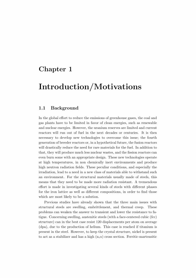
The idea to solve the problem would be to follow this iterative scheme:

first, an electronic density is stated. From this density, all the functionals

are determined, which allows us to solve the Kohn-Sham equations. This

gives the new orbitals, and a new density is calculated. This algorithm is

running until the density converges. It is illustrated in Figure2.1.

𝜌0(𝑟 )

ν𝐾𝑆(𝑟 )

−1

2∇2 + ν𝐾𝑆(𝑟 ) ψ𝑖 = 𝜀𝑖 ψ𝑖

𝜌(𝑟 )= ψ𝑖(𝑟 )𝑀𝑖

Convergence?

End

No

Yes

Figure 2.1: Flow-chart of a typical DFT calculation within the Kohn-Sham

framework.

It is worth noting that until now, the equations are exact. Unfortunately,

the real exchange-correlation energy is not known and it is necessary to

make some approximations here. These approximations have to be precise

and not to require too much calculation power. Over the past few years, a


lot of different methods have been proposed, some of which, used or leading

to the ones used in this work, are presented now.

2.1.1.4 The Local Density Approximation (LDA)

This approximation states that the exchange correlation energy of the sys-

tem is locally determined only by its electronic density. To each point of

space is corresponding a density and therefore an exchange-correlation en-

ergy. This is the simplest approach, which find root in the 1920′s. Indeed,

most of the LDA approaches have been derived from the Homogeneous Elec-

tron Gas theory of Thomas-Fermi. Under this hypothesis, the kinetic and

exchange energies for non-interacting system are known.

T [ρ] = 2.87

∫ρ5/3(r)dr (2.11)

EX [ρ] = 0.74

∫ρ4/3(r)dr

Finding the correlation energy is harder and numerous different attempts

exist (VWN, PZ81, CP, PW92, ...). The LDA approximation gives strikingly

accurate results due to a cancellation of different errors [15][18]. However, it

is possible to find a better approximation without increasing too much the

calculation time.

2.1.1.5 The Generalized Gradient Approximation (GGA)

This approximation extends the LDA by considering the surrounding elec-

tronic density before calculating the exchange correlation energy in a specific

place. The exchange-correlation energy is then described as in equation 2.12.

EXC =

∫ρ(r)εXC(ρ,∇ρ)dr (2.12)

For this kind of functionals, the pragmatism is favored over the physical

meaning. The functional is modified in an arbitrary way to respect the

boundary conditions, and only its performance matters. This conducted

Koch and Holthausen to say that “Some of these functionals are not even

based on any physical model” [19].

Again, a lot of different functionals have been developed (PW91, PBE,

B3LYP) and have advantages and drawbacks depending on the properties

of interest [18].

To go even further, some functionals take into account the second deriva-

tive of the electronic density (Meta-GGA functionals), or mix a non-interacting

approach with a fully interacting one (Hybrid Exchange Functionals).


2.1.1.6 The Perdew Burke Ernzerhof potential (PBE)

The Perdew Burke Ernzerhof potential is a modified GGA potential in which

all parameters are fundamental constants [20]. It is a simplification of the

PW91 potential which fits only the most relevant conditions on an energy

level and is hence easier to understand, derive, and implement. This func-

tional keeps the correct properties from the LDA and adds others such as

superior limits for the exchange and the correlation energies but neglects a

few aspects, including the second order gradient coefficients for EX and ECin the slowly varying limit. The choice of the correct properties has been

made depending on what seemed the most important on an energy level.

The PBE potential is the one that has been used for all the simulations

in this thesis, using the potential data bank of VASP.

2.1.2 Wavefunctions

Having good representations of the wavefunctions is essential since they are

used in the iterative process to determine the density. Hence, they have to

be as precise as possible. However, determining a good way to represent the

wavefunctions can be tricky, this representation having to be both realistic

and computationally efficient in any part of space.

In this work, the Projector Augmented Wave method has been used.

Various papers can be consulted for more information [21][22].

2.1.2.1 Pseudopotential methods

These methods use plane waves, as defined by equation 2.13.

Φi(r) =∑K

ci,Kei(k+K).r (2.13)

If fitting the real wavefunction with plane waves is really computationally

efficient in the areas far from a nucleus, it needs a huge basis set in the core

region to be convergent, since the real wavefunction varies quickly. However,

most of the physical properties are defined by the valence electrons and the

nuclei part can be thought as not changing in different environments (frozen

core approximation). For this reason, the pseudopotential method consists

in fitting to the reality in the valence region, but modifying the wavefunction

in the core region to soften it (Figure 2.2) and fasten the convergence.

The cut-off radius (rc) has to be chosen such as the potential is converg-

ing quickly (higher radius) but is still usable for systems with a different


Figure 2.2: Illustration of the pseudopotential and of the pseudo wavefunc-

tion.


environment, that is to say that the unvarying frozen core should not be too

big (lower radius).

The main advantage of this method is to reduce the number of electrons

of interest, considering only the valence ones, and doing so, increasing the

size of a studied system for the same computation time. Another advantage

is to reduce the basis set size, and therefore to speed up the calculations.

However, these wavefunctions should be norm-conserving and ultrasoft pseu-

dopotentials, which don’t have to respect this condition, have been proposed

by Vanderbilt [23] to further reduce the basis set.

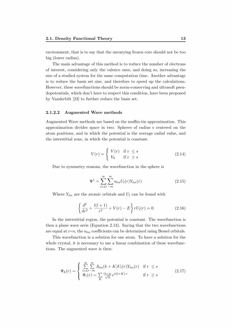
2.1.2.2 Augmented Wave methods

Augmented Wave methods are based on the muffin-tin approximation. This

approximation divides space in two: Spheres of radius s centered on the

atom positions, and in which the potential is the average radial value, and

the interstitial zone, in which the potential is constant.

V (r) =

V (r) if r ≤ sV0 if r ≥ s

(2.14)

Due to symmetry reasons, the wavefunction in the sphere is

Ψ1 =∞∑l=O

m∑−m

almUl(r)Ylm(r) (2.15)

Where Ylm are the atomic orbitals and Ul can be found withd2

dr2+l(l + 1)

r2+ V (r)− E

rUl(r) = 0 (2.16)

In the interstitial region, the potential is constant. The wavefunction is

then a plane wave serie (Equation 2.13). Saying that the two wavefunctions

are equal at r=s, the alm coefficients can be determined using Bessel orbitals.

This wavefunction is a solution for one atom. To have a solution for the

whole crystal, it is necessary to use a linear combination of these wavefunc-

tions. The augmented wave is then:

Ψk(r) =

∞∑l=O

m∑−m

Alm(k +K)Ul(r)Ylm(r) if r ≤ s

Φi(r) =∑K

ck+K√Ωei(k+K).r if r ≥ s

(2.17)


2.1.2.3 Projector Augmented Wave method (PAW)

It is a mix between the pseudo potential and the augmented wave meth-

ods. In the core region, the wavefunction is expressed with the help of the

atomic orbitals (from the augmented wave method) and in the valence zone,

plane waves are used (from the pseudopotential method). This allows an

equivalent speed of calculation with more precise results.

To avoid having to calculate two sets of wavefunctions, auxiliary wave-

functions which can get derived from the real wavefunctions by a linear

transformation are used. This linear transformation is such that in the

valence region it becomes the identity. In the core region, the real wave-

functions can be obtained by adding to the identity the projection of the

auxiliary set on the atomic orbitals of the atom with all its electrons, and

substracting the same projection on the atomic orbitals of an atom with

just the valence electrons, to avoid counting it twice (once from the identity,

once from the projection).

|ψn〉 = |ψn〉+∑a

(∑i

|φai 〉〈pai |ψn〉 −∑i

|φai 〉〈pai |ψn〉

)(2.18)

where ψn and ψn are the real and auxiliary wavefunction, φai and φai the

atomic orbitals of the atom with all the electrons and with only the valence

electrons, pai is the projector, and a represents the atoms.

2.1.3 Vienna Ab-initio Simulation Package

For all the DFT calculations in this work, the Vienna Ab-initio Simulation

Package (VASP) has been used. The chosen potentials are PBE used with

the Projector Augmented Wave method. The energy cut-off for the basis set

has been chosen to be 450 eV due to the presence of oxygen in the systems

of interest. It has been shown that there is no significant change when this

cut-off is set to an higher value, except for a much larger calculating power

required.

VASP uses periodic boundary conditions, that is to say that the supercell

repeats itself. Again, it is important to choose a supercell big enough to

avoid too big boundary effects, but it has to be small enough so it will not

take an unreasonable time to reach convergence. Unless otherwise specified,

the simulations have been made using a supercell of 250 base atoms and

a sampling of the Brillouin zone with 27 points. To help convergence, an

electronic temperature has been used (through the parameter SIGMA, 0.3

2.2. Kinetic Monte Carlo 15

in this work). These parameters have been chosen high enough to reach a

convergence of the free energy and low enough to keep a calculation time

under 24 hours.

Most of the simulations have been run in two steps, one to reach a near-

convergence state with specific parameters to accelerate the simulation while

loosing some accuracy, and one to converge and obtain accurate data from

this state with the above-mentioned parameters.

2.1.3.1 Nudged Elastic Band (NEB) method

In order to simulate a dynamic system, it is necessary to find data for the

diffusion of atoms. This value is the migration energy and is found by com-

puting the minimum energy path (MEP) between two stable configurations.

It is found combining the density functional theory with the nudged elastic

band method. It would have been possible to use other methods [24], such

as the slowest ascent path [25] (drag method).

The idea with the NEB (chain-of-states method) is to calculate the equi-

librium state of the system in an initial and a final geometric configuration

using a DFT code. Then, a certain amount of images are created, moving

progressively the atoms which are not in the same position in the two states.

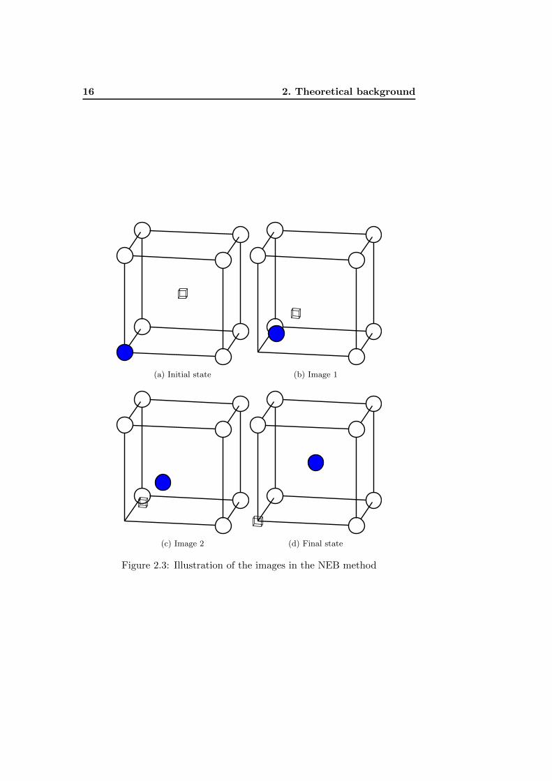
This motion is linear in function of the number of images asked. In figure

2.3 are shown two images between one state with a blue atom first nearest

neighbour from a vacancy and a final state where both of them have ex-

changed their positions. Obviously, the vacancy is not physically moving,

since it represents an absence of atom.

Once the images are defined, a DFT calculation is run for each of them,

and they are relaxed. However, they are constrained by strings, which force

the distances between each other to remain equal [26]. This is done by

projecting out the perpendicular component of the spring force and the

parallel component of the true force [27].

2.2 Kinetic Monte Carlo

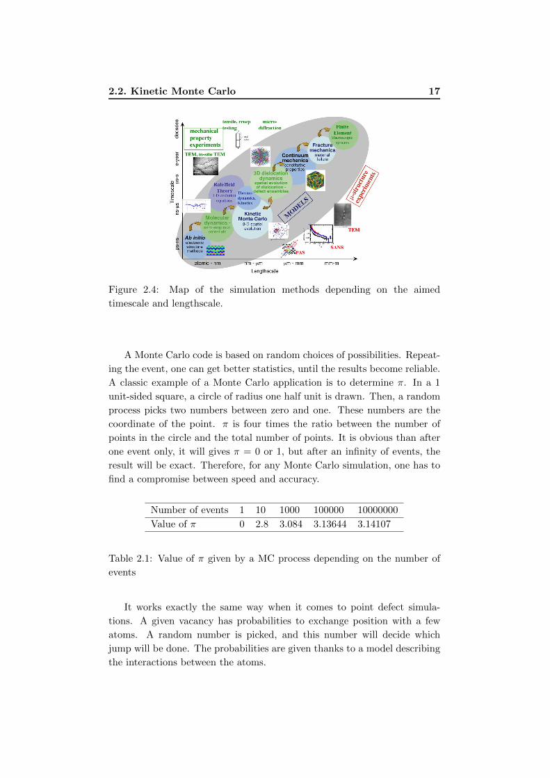
One of the main drawbacks of the DFT is that the time scale is limited

to a few nanoseconds, and the length scale to few nanometers. It is then

necessary to use another method to have results for a longer time or a bigger

material. Numerous ways of doing so exist (FIG 2.4), but in this thesis, a

kinetic Monte Carlo code has been used.


(a) Initial state (b) Image 1

(c) Image 2 (d) Final state

Figure 2.3: Illustration of the images in the NEB method


Figure 2.4: Map of the simulation methods depending on the aimed

timescale and lengthscale.

A Monte Carlo code is based on random choices of possibilities. Repeat-

ing the event, one can get better statistics, until the results become reliable.

A classic example of a Monte Carlo application is to determine π. In a 1

unit-sided square, a circle of radius one half unit is drawn. Then, a random

process picks two numbers between zero and one. These numbers are the

coordinate of the point. π is four times the ratio between the number of

points in the circle and the total number of points. It is obvious than after

one event only, it will gives π = 0 or 1, but after an infinity of events, the

result will be exact. Therefore, for any Monte Carlo simulation, one has to

find a compromise between speed and accuracy.

Number of events 1 10 1000 100000 10000000

Value of π 0 2.8 3.084 3.13644 3.14107

Table 2.1: Value of π given by a MC process depending on the number of

events

It works exactly the same way when it comes to point defect simula-

tions. A given vacancy has probabilities to exchange position with a few

atoms. A random number is picked, and this number will decide which

jump will be done. The probabilities are given thanks to a model describing

the interactions between the atoms.


2.2.1 Atomic Kinetic Monte Carlo

A atomic Monte Carlo methods means that the different atoms are bound to

the lattice positions. One have to be aware that this method doesn’t support

high disturbances of the lattice. It could be a problem here since some of

the nanoclusters studied have a completely different lattice parameter than

the one of α-iron, but since these clusters keep a small size in the nucleation

stage, the condition is supposed to be met [11].

To have a notion of kinetics one needs a time-step, which in this method

is defined as the inverse of the sum of the migration probabilities by second,

given by the residence time algorithm. The theoretical determination of the

time-step is usually done in the framework of the Transition State Theory

[28]. In this framework,

ΓX,V = νXexp

(−EakT

)(2.19)

where Γ is the migration probability by second, that’s to say the prob-

ability that an atom and a vacancy V exchange their positions during the

step X, ν is the attempt frequency which depends on the type of atom and

the temperature, k is the Boltzmann constant, T the temperature and Eathe activation energy for the jump defined (Eq 2.20) and modeled (Eq 2.21)

as

Ea = ESaddlePoint − Ei. (2.20)

Ea = E?m +Ef − Ei

2. (2.21)

E?m is the migration energy of a vacancy with the first neighbour atom.

One is defined for each type of atom and for the jump of an interstitial

atom; For the case of oxygen, the migration energy is defined between two

first nearest neighbour octahedral positions. Ef and Ei are the final and

initial energies. This equation allows us to not need to calculate every

migration energy with a Nudged Elastic Band (NEB) method, which would

be time-prohibitive.

ν can be determined with a relative precision by

ν =

∏Ni ω

starti∏N−1

i ωsaddlei

(2.22)

where ωstarti and ωsaddlei are the frequencies of the entire system at equi-

librium and the frequencies of the entire system except the jumping atom

when this one is at the saddle point. Usually, ν is around 10−12.


The time-step for one vacancy at one step can then be calculated as

∆tX,V =1∑

X,V ΓX,V(2.23)

However, the system has to be at the thermodynamical equilibrium for

this formula to be usable. Unfortunately, the equilibrium concentration of

vacancies is so low that even with only one, the system is over saturated.

The time-step has to be corrected to account for this.

∆t′

=CV

CeqV (T )∆t

′(2.24)

where the equilibrium concentration of vacancies at the temperature T

can be found using the Gibbs energy (Eq 2.25 [29]) and ∆t′

is the corrected

time-step.

CeqV (T ) = e−

GfkbT (2.25)

where kb is the Boltzmann constant and Gf is the Gibbs energy of va-

cancy formation.

2.2.2 LAttice KInetic MOnte CArlo

In the context of this thesis, the Monte Carlo code used is LAKIMOCA

(LAttice KInetic MOnte CArlo). It is written by C. Domain at Electricite

de France. It was started in 1998 and is still under development.

This code can read numerous types of potential, and the one used here

was of type Embedded Atom Model [30]. It has been run using an iron

lattice of 42*42*42 cells, with chromium, titanium, yttrium in substitutional

positions, oxygen atoms in octahedral positions and one vacancy.

For each step, the code will consider the vacancies, the Self Interstitial

Atoms (SIA) and the Foreign Interstitial Atoms (FIA) and calculate the

probabilities of these to jump, depending on the surroundings. Then, it will

randomly pick a jump for each of those. Once this has been done for all the

defects, a new step is launched.

The other parameters are the jump attempt frequency, the temperature,

the lattice parameter, the number of steps and a seed for the random number

generator.


2.3 Materials irradiation

2.3.1 Defects

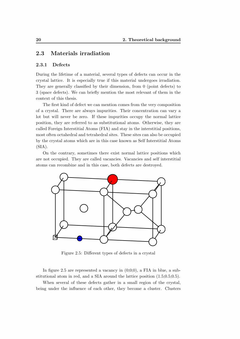
During the lifetime of a material, several types of defects can occur in the

crystal lattice. It is especially true if this material undergoes irradiation.

They are generally classified by their dimension, from 0 (point defects) to

3 (space defects). We can briefly mention the most relevant of them in the

context of this thesis.

The first kind of defect we can mention comes from the very composition

of a crystal. There are always impurities. Their concentration can vary a

lot but will never be zero. If these impurities occupy the normal lattice

position, they are referred to as substitutional atoms. Otherwise, they are

called Foreign Interstitial Atoms (FIA) and stay in the interstitial positions,

most often octahedral and tetrahedral sites. These sites can also be occupied

by the crystal atoms which are in this case known as Self Interstitial Atoms

(SIA).

On the contrary, sometimes there exist normal lattice positions which

are not occupied. They are called vacancies. Vacancies and self interstitial

atoms can recombine and in this case, both defects are destroyed.

Figure 2.5: Different types of defects in a crystal

In figure 2.5 are represented a vacancy in (0;0;0), a FIA in blue, a sub-

stitutional atom in red, and a SIA around the lattice position (1.5;0.5;0.5).

When several of these defects gather in a small region of the crystal,

being under the influence of each other, they become a cluster. Clusters

2.3. Materials irradiation 21

can dramatically modify the mechanical behaviour of a material, as will be

explained more in details in part 2.3.3.

This work is mainly aimed on these point defects, but also dislocations

[31], grain boundaries [32] and clusters can be mentioned.

2.3.2 Energies

In the context of this thesis, the point defects have been well studied. To

do that, it is necessary to define some energies. These energies will give

information on if a crystallographic configuration is stable or if a trans-

formation is thermodynamically favoured. As such, it is crucial to have a

precise definition for each.

• The cohesive energy: it is the difference between the energy of a solid

and the energy of the isolated atoms. It represents the force acting

against the seperation of the atoms. It can be calculated thanks to

the following formula.

Ecoh = Etot −∑N

Eiso (2.26)

• The binding energy: When there exists more than one defect in a

lattice, one can quantify the influence of one defect on the other one.

To do so, the energy associated to the neighbouring of these two defects

is calculated (Eq. 2.27) as the difference between the energy of a

crystal where the defects are close and the same crystal where the

defects are far from each other.

Eb = EtotA − EtotB (2.27)

Where the configuration A is the one with the defect close and the B

is the one with far from each other defects.

However, since for computational reasons, it is not always possible

to put defects at a long enough distance to consider that they have

absolutely no effect on each other, the Eq. 2.28 is often used. The

defects are taken alone in an otherwise perfect lattice. The result is

the same as if it was possible to set the defect at an infinite distance

in the same system.

Eb = Etot + Eref − Edefect1 − Edefect2 (2.28)


This equation can be generalized to N defects as

Eb = Etot + (N − 1)Eref −Edefect1 −Edefect2 − ...−EdefectN (2.29)

• The migration energy: To simulate the kinetics of a system, the mi-

gration energy is an important value. It represents the barrier that an

atom needs to pass in order for the system to go from one stable state

to another. Stable positions have local energy minima and therefore,

the energy of the atom will be higher on the migration path. We call

the saddle point the point where the atom have the highest energy on

the path of lowest energy. The difference in energy between the sad-

dle point and the starting point is the migration energy. The saddle

energy is found by determining the MEP, thanks to methods such as

the NEB one.

2.3.3 Macroscopic effect of irradiation

Under irradiation, due to the high energy neutron flux received by the ma-

terial, there is a multiplication of point defects. Indeed, the energy of the

incoming neutrons is several orders of magnitude greater than the threshold

displacement energy of the atoms (order of magnitude of 1 MeV for the neu-

tron against several tens of eV for the threshold) and so, each neutron will

generate a collision cascade in the material, resulting in the creation of nu-

merous defects such as Frenkel pairs, which number is estimated in equation

2.30 [33]. Most of these defects will recombine and only 20% to 30% will

survive [34], but the remaining ones will drastically change the macroscopic

properties of the material. Among various effects which can be read more

in details in Recent Development in Irradiation-Resistant Steels [35], some

deserve to be mentioned.

NFP = 0.8EnETres

(2.30)

where NFP is the number of Frenkel pairs, En and ETres are the neutron

energy and the threshold displacement energy.

2.3.3.1 Swelling

Swelling in structural materials is a major problem in reactors since it will

limit the performances of the reactor core. It will occur in two steps; the

first one, or incubation stage, is quite slow and is due to the cavity formation


and grain growth. This phase duration depends on various parameters like

the temperature or the dose rate. The solute concentrations also play an

important role and will be further detailed. The second phase is faster and

causes a swelling of about 1% per dpa (Displacement Per Atom: 1 dpa means

that every atom has been moved from its initial position once on average)

for stainless steels due to the formation of helium bubbles. The incubation

period has been observed to be the shortest at around 750 K for a SS316

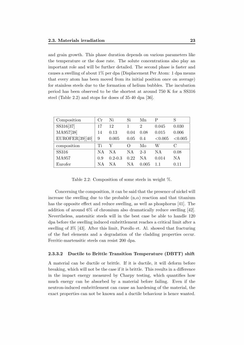
steel (Table 2.2) and stops for doses of 35-40 dpa [36].

Composition Cr Ni Si Mn P S

SS316[37] 17 12 1 2 0.045 0.030

MA957[38] 14 0.13 0.04 0.08 0.015 0.006

EUROFER[39][40] 9 0.005 0.05 0.4 <0.005 <0.005

composition Ti Y O Mo W C

SS316 NA NA NA 2-3 NA 0.08

MA957 0.9 0.2-0.3 0.22 NA 0.014 NA

Eurofer NA NA NA 0.005 1.1 0.11

Table 2.2: Composition of some steels in weight %.

Concerning the composition, it can be said that the presence of nickel will

increase the swelling due to the probable (n,α) reaction and that titanium

has the opposite effect and reduce swelling, as well as phosphorus [41]. The

addition of around 6% of chromium also dramatically reduce swelling [42].

Nevertheless, austenitic steels will in the best case be able to handle 120

dpa before the swelling induced embrittlement reaches a critical limit after a

swelling of 3% [43]. After this limit, Porollo et. Al. showed that fracturing

of the fuel elements and a degradation of the cladding properties occur.

Ferritic-martensitic steels can resist 200 dpa.

2.3.3.2 Ductile to Brittle Transition Temperature (DBTT) shift

A material can be ductile or brittle. If it is ductile, it will deform before

breaking, which will not be the case if it is brittle. This results in a difference

in the impact energy measured by Charpy testing, which quantifies how

much energy can be absorbed by a material before failing. Even if the

neutron-induced embrittlement can cause an hardening of the material, the

exact properties can not be known and a ductile behaviour is hence wanted.


The problem here is that irradiation causes a shift of the DBTT and a

material which is originally ductile can become brittle after a few years. The

order of magnitude of the shift for an EUROFER steel (see table 2.2) is of

200-250 K for dpa ranging from 30 to 80 at around 600 K. The dose rate

is not indicated [36]. Austenitic steels have on this point a huge advantage

since they will stay ductile at room temperature until after the swelling

becomes an issue. On the other hand, ferritic-martensitic steels will become

brittle after a few dpa. This problem is exacerbated for low irradiation

temperature but can be reduced with a concentration of 9% of chromium

[36] as it is shown on picture 2.6. The presence of Ni leads to a larger amount

of He atoms in the iron matrix under irradiation, which causes a larger shift

of the DBTT [44].

Figure 2.6: Influence of the chromium content on the DBTT shift.

2.3.3.3 Creep rupture embrittlement

When a material undergoes irradiation, its resistance to creep progressively

decreases. The creep rupture time can be expressed in function of the pres-

sure and the temperature as

P = T (A+ log(tr)) (2.31)

where T is the temperature in kelvin, tr is the rupture time, P is the


Larson-Miller parameter and A is a constant. Both P and A depends on the

pressure and on the material.

The creep rupture time is much longer for austenitic steels than for

ferritic-martensitic steels and decreases when the irradiation is done at high

temperature [36][45]. The creep resistance can also be enhanced by the

addition of W and Nb [46].

2.3.4 Oxide Dispersion Strengthened (ODS) steels

As seen in the previous part, both austenitic and ferritic-martensitic steels

have resistance problem when they are under irradiation for a long time,

and this no matter what the temperature is. Efforts that have been made to

change the composition including for instance titanium or chromium have

given reasonably good results, but this is still not satisfying for GEN IV

fission or fusion usages. However, the three above mentioned issues can be

significantly reduced by the use of ODS steels.

2.3.4.1 Principle

The principle here is to add to the steel some other atoms, which will create

a large amount of nano-scaled precipitates, around 1024.m−3 [47]. The steel

and the wanted components of the nanoclusters are mechanically alloyed

(MA) by ball milling. Typically, the created nano-ferritic alloy will contain

yttrium, titanium, tungsten, chromium and oxygen.

The chromium is useful to increase the resistance of the steel to oxidation

and corrosion, while the tungsten will be beneficial to improve the strength of

the steel, forming solid solutions. Yttrium, titanium and oxygen cluster and

prevent dislocations from moving. Titanium can be replaced by zirconium

for a higher stability [7]. Depending on the composition of the alloy and of

the temperature of the heat treatments, nanoclusters are ranging between 1

nm and 2 nm of radius, and have a volume fraction between 0.4% and 2%.

The composition of the clusters can also vary from near equilibrium oxides

like Y2TiO5 or be a bit further, like Y2Ti2O7 or Y2TiO3 [35].

2.3.4.2 Known results

When not under irradiation, the ODS steels exhibits a high tensile and

creep strength and a rather good tensile ductility. Their low-cycle fatigue

properties are also excellent [35]. However, the behaviour under irradiation

is what is of main interest.


It has been found that irradiation -up to 150 dpa at 975 K and 10−3

dpa/s using 6.4 MeV Fe3+ions- doesn’t affect significantly nanoclusters [48].

A prolonged exposure to high temperature doesn’t cause coarsening even

after 14500 hours at 800C [47].

Those nanoclusters trap helium that is generated into small bubbles and pre-

vent the material from swelling in a significant way [49]. Thus, the swelling

induced embrittlement is reduced. The very high density of nanofeatures

as well as the obstacles due to irradiation trap the dislocation loops. Due

to this pinning, the dislocation density is 10 times higher compared to the

ODS steels without (Y,Ti,O) clusters and the creep rate at around 1000 K is

reduced by 6 orders of magnitude [47]. Losses of ductility due to irradiation

are also reduced compared to martensitic steels [50], and the presence of Cr

in the ODS steel reduces the shift further [51].

Chapter 3

Results

In this section are reported the results of this thesis. They are divided into

two parts; the ones coming from the ab initio calculations and the ones

coming from the Monte Carlo simulations.

In the first-principles chapter, the focus is first given on finding the stable

position for each considered atom in a BCC iron lattice. Then, the inter-

actions between the solutes and the vacancies are treated. In the following

part, migration energies are computed. Thereafter, interactions between two

solutes will be studied. From all of these data, the possibility of forming

a cluster and simple mechanisms for the formation will be discussed. The

peculiar attraction of oxygen atoms toward a vacancy as well as the unex-

pected diffusion mechanism for the yttrium atom will be developed in more

details.

Then, in the atomistic kinetic Monte Carlo part, all the parameters from

the ab-initio simulations will be used to

• study the formation of nanoclusters

• study the stability of these clusters under normal conditions

3.1 Ab-initio calculations

These ab initio simulations (described in the theoretical background part)

only depend on the choice of approximations for the Hamiltonian and for

the wavefunctions. Hence, a good accuracy can be expected for the results.

All these first-principles calculations have been made using VASP, and the

details about the configuration are given in the section 2.1.3, and have been

chosen so that a convergence is reached. The simulations of this work are

supposedly more precise that what can be found in the literature since the

28 3. Results

sampling of the Brillouin zone is denser, the supercell bigger and the energy

cut-off higher.

One has to be aware that all of the data presented in this part are only

valid in the dilute limit. When the concentration of a solute becomes too

high, new phenomena start and modify the behaviour of the solute. For

instance, Cr will cluster if its concentration is higher than a few percents.

3.1.1 stable position of solutes

In order to calculate the binding energies between two defects in the iron

lattice, it is necessary to have the solution energy of these solutes in the

stable position. To do that, the cohesive energy of each atom is calculated

either in the reference crystal (for Cr, Ti and Y) or in a dimer (for O) and

are listed in table 3.1. The stable position can be found trying to put the

atom in different sites and checking for which the energy is the lowest. On

the figure 3.1 are the tensile (in red), compressed (in blue) and mixed (in

green) site of a cell when there is a self interstitial atom (SIA) in the plane

[110], as described by Olsson et. Al. [5].

Figure 3.1: Tensile, compressed and mixed sites.

These configurations have been found more stable for iron than the ones

with an SIA in the octahedral or tetrahedral sites. It is worth being explored

3.1. Ab-initio calculations 29

for Ti, Cr and Y also. The values found are reasonably close from the

literature, which confirms the model. An exception to that is the oxygen

data. However, no-one in the literature explains where the cohesive energy

they use has been found. In this work, a magnetic dimer has been used.

Using a different cohesive energy can lead to different solution energies, but

these values are not primordial for the next steps, since a difference in energy

is used to calculate any binding energy. For this reason, the comparison

criteria should be the difference in energy between the octahedral and the

tetrahedral sites. It can also be noticed a big difference with C. C. Fu values

which seem a bit under-evaluated, probably due to the fact that she used a

different code.

The results shown in the table 3.1 prove that Ti, Cr and Y are more stable

in a substitutional site and oxygen is found more stable in the octahedral

site, by 0.51 eV compared to the tetrahedral position in confirmation of

Murali’s work and infirming Jiang’s one where a mistake has probably been

made. The binding energies are also indicated in table 3.2 for a SIA and

a substitutional solute. The only attractive one is the tensile, which was

expected since the [110] dumbbell makes the compressed sites closer and the

tensile sites further from the SIA than if there was no defect.

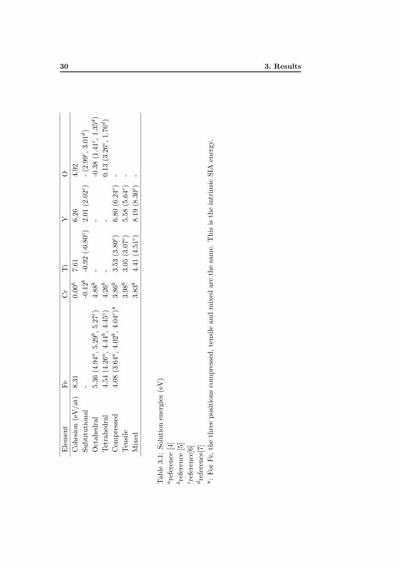
30 3. ResultsE

lem

ent

Fe

Cr

Ti

YO

Coh

esio

n(e

V/at

)8.

31

0.00b

7.61

6.26

4.92

Su

bti

tuti

on

al

--0

.12b

-0.9

2(-

0.80c)

2.01

(2.0

2c)

-(2

.99c,

3.01d)

Oct

ahed

ral

5.36

(4.9

4a,

5.29b,

5.27c)

4.88b

--

-0.3

8(1

.41c,

1.3

5d)

Tet

rah

edra

l4.

54

(4.2

6a,

4.44b,

4.45c)

4.26b

--

0.13

(3.2

6c,

1.7

6d)

Com

pre

ssed

4.08

(3.6

4a,

4.02b,

4.04c)*

3.86b

3.53

(3.8

0c)

6.80

(6.2

4c)

-

Ten

sile

3.98b

3.05

(3.0

7c)

5.58

(5.6

4c)

-

Mix

ed3.

83b

4.41

(4.5

1c)

8.19

(8.3

0c)

-

Tab

le3.

1:S

olu

tion

ener

gie

s(e

V)

are

fere

nce

[4]

bre

fere

nce

[5]

cre

fere

nce

[6]

dre

fere

nce

[7]

*:F

or

Fe,

the

thre

ep

osit

ion

sco

mp

ress

ed,

ten

sile

and

mix

edar

eth

esa

me.

Th

isis

the

intr

insi

cS

IAen

ergy.


Element Cr Ti Y

Compressed 0.05a -0.35 -0.72

Tensile -0.07a 0.13 0.50

Mixed 0.08a -1.23 -2.11

Table 3.2: Binding energies SIA-solute(eV)areference[5]

3.1.2 Interactions with vacancies

The interactions between the solutes and the vacancies are of prime im-

portance. Indeed, the migration mechanism for the solutes occupying the

substitutional positions is based on the vacancies according to the work of

Le Claire [10] when their diffusion rate is of the same order of magnitude

as the one of the host. In this study, this is at least the case for Cr and

Ti, but it is less direct for Y. Moreover, a great quantity of vacancies are

created during the irradiation process, hence determining their behaviour is

necessary.

The first step is to determine precisely the geometry used. In most of

the cases, the interaction will be negligible after a length corresponding to

the diagonal of a primary BCC cell (as represented in Figure 3.2). In some

rare cases, the calculations have been pursued further for reasons that will

be explained. In Figure 3.2.a are represented the five nearest substitutional

neighbours for a regular lattice position, and in figure 3.2.b the five nearest

octahedral positions. Their distances are summed up in table 3.3.

Nearest neighbour 1st 2nd 3rd 4th 5th

Subtitutional 0.87 1.00 1.41 1.58 1.73

Octahedral 0.50 0.70 1.12 1.22 1.5

Table 3.3: Distance between the nearest neighbours (in unit of lattice pa-

rameter

Chromium and titanium have a negative solution energy in a substitu-

tional lattice position, which means that they are even more stable than an

iron atom in these sites. It is therefore a normal behaviour to be repulsive

with a defect, if it directly tries to change the position of the substitutional

atom, hence the repulsive attraction with a vacancy in first nearest neigh-

bour. On the other hand, yttrium is much bigger than iron, and the vacancy

32 3. Results

5

14

2

3

(a) substitutional

4

5

1

23

(b) octahedral

Figure 3.2: 5 nearest octahedral position from a regular lattice site


Element Cr Ti Y O

1NN -0.24 0.24b (0.26a) 1.27 (1.45a) 1.69 (1.65a,1.45c)

2NN 0.00 -0.17b (0.16a) 0.20 (0.26a) 0.73 (0.75a, 0.60c)

3NN -0.01 0.01b 0.13 0.14

4NN -0.03 0.00b 0.04 0.37

5NN 0.01 0.01b 0.20 0.01

Table 3.4: Binding energies with a vacancy.areference[6]breference[52]creference[8]

offers it the possibility to relax from the lattice position and increase the dis-

tance with the surrounding iron atoms. As a consequence, they are strongly

binding. This interaction will be studied with more details in section 3.1.3.

The analysis of the strong attraction between oxygen and a vacancy will

also be deepened.

In a more general view, the strength of the interaction decreases when

the foreign atom and the vacancy get further away from each other. Since

yttrium is so big, its range of effect is far-reaching and permits some consid-

erations on the geometry. The interaction with the fifth nearest neighbour is

indeed stronger than the one with the forth. It can be explained by what is

between the two defects in the crystal. In the case of the 5NN, there is only

one atom, which can relax and allow the yttrium to relax in turn, whereas

for the 4NN, the iron atoms corresponding to 1 and 2 on the picture 3.2.a

will be on the way.

Chromium repels the vacancies in first nearest neighbour position. This

will decrease the mobility of Cr atoms, since they are moving thanks to the

vacancy diffusion mechanism. At longer distances, they are almost trans-

parent to vacancies.

Titanium binds with the vacancy in first nearest neighbour, but repulses it

in second nearest neighbour, while being transparent at longer distances.

This results in both a difficulty for the vacancy to approach, and then to

move away, which will also decrease the mobility. However, for both Cr and

Ti, the binding energies are not that strong and will not prevent a displace-

ment.

For yttrium on the other hand, the attractive energies in second and es-

pecially in first nearest neighbour with the vacancy are so strong that the

vacancy is unlikely to move away. This drastically reduces the mobility of

34 3. Results

Y atoms. It must also be added that the interaction between Y and a va-

cancy has a much longer range than for Cr and Ti which will have for effect

to attract a vacancy jumping around from further, and therefore make the

yttrium act as a vacancy trap.

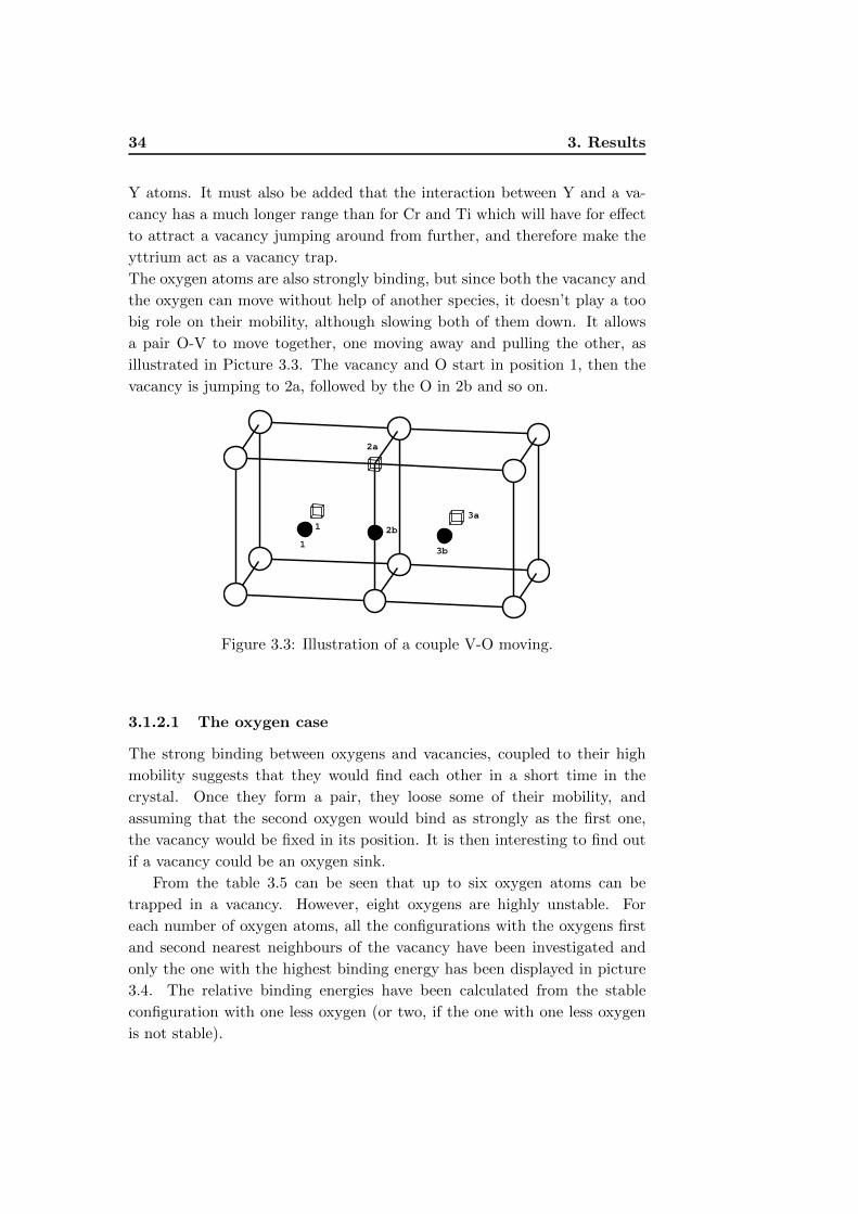
The oxygen atoms are also strongly binding, but since both the vacancy and

the oxygen can move without help of another species, it doesn’t play a too

big role on their mobility, although slowing both of them down. It allows

a pair O-V to move together, one moving away and pulling the other, as

illustrated in Picture 3.3. The vacancy and O start in position 1, then the

vacancy is jumping to 2a, followed by the O in 2b and so on.

1

3a

1

2b

3b

2a

Figure 3.3: Illustration of a couple V-O moving.

3.1.2.1 The oxygen case

The strong binding between oxygens and vacancies, coupled to their high

mobility suggests that they would find each other in a short time in the

crystal. Once they form a pair, they loose some of their mobility, and

assuming that the second oxygen would bind as strongly as the first one,

the vacancy would be fixed in its position. It is then interesting to find out

if a vacancy could be an oxygen sink.

From the table 3.5 can be seen that up to six oxygen atoms can be

trapped in a vacancy. However, eight oxygens are highly unstable. For

each number of oxygen atoms, all the configurations with the oxygens first

and second nearest neighbours of the vacancy have been investigated and

only the one with the highest binding energy has been displayed in picture

3.4. The relative binding energies have been calculated from the stable

configuration with one less oxygen (or two, if the one with one less oxygen

is not stable).


(a) 1 oxygen (b) 2 oxygens

(c) 3 oxygens (d) 4 oxygens

(e) 6 oxygens (f) 8 oxygens

Figure 3.4: Geometry of vacancy-oxygen clusters.

36 3. Results

Number of oxygen Binding energy Relative binding energy

1 1.69 -

2 3.50 1.81

3 3.83 0.33

4 4.01 0.18

6 5.88 1.87

8 -6.71 -12.59

Table 3.5: Binding and relative binding energies of oxygens with a vacancy.

For V-O2, the two oxygens relax and form a dumbbell around the lattice

position with no iron atom. The configuration with 3 O is the only one

stable without being symmetric; no configuration with 5 O (not represented

here) has been found stable either. Except for the V-O5 system, all the

systems for which the oxygen relaxation is toward the vacancy or negligible

are binding, and the one with a relaxation in the opposite direction are

repulsive (See picture 3.5). The V-O3 system breaks a bit the trend, due to

the non-symmetry.

1 2 3 4 5 6 7 8−0.1

−0.08

−0.06

−0.04

−0.02

0

0.02

0.04

0.06

0.08

0.1

Number of oxygens

Re

laxa

tio

n /

la

ttic

e p

ara

me

ter

[%]

Figure 3.5: Relaxation of the oxygen atoms around a vacancy.

In the figure 3.6 are represented the differential charge densities of an

iron matrix with one vacancy and one oxygen, and of an iron matrix with

one vacancy and six oxygens. The differential charge density is defined as

the difference between the charge density of the studied system and the

charge density of each atom alone.


(a) V-O (b) V-O6 (c) V-O6

Figure 3.6: Differential electron density for 1 and 6 octahedral O around a

vacancy.

The picture a. shows that O and V have a completely opposite charge,

which suggest that they form an attractive ionic pair. Indeed, the binding

energy between them is 1.69 eV. The picture b. proves that the charge

is spatially confined around the vacancy. The charge cage present around

a vacancy in an iron matrix [52] has not been strongly perturbed by the

presence of oxygens (Fig c.). That can explain the binding character of this

cluster.

3.1.3 Migration of the solutes

The migration energy of a solute in the iron host can be estimated by finding

the Minimum Energy Path (MEP) thanks to a method such as the Nudged

Elastic Band (NEB) one. This method is described in section 2.1.3.1. The

diffusion mechanism considered for the solutes occupying the substitutional

positions is the vacancy mechanism, and for oxygen, the jump between two

octahedral positions, passing by a tetrahedral one.

The simulations have been done using 5 images in a supercell of 128

atoms with an energy cut-off of 450 eV and 27 K points. The results are

displayed in table 3.6.

Element Fe Cr Ti Y O

Migration energy 0.65 0.52 0.35 see section 3.1.3.1 0.48

Table 3.6: Migration energies of solutes in an iron BCC lattice.

The iron host has the highest barrier for the vacancy assisted migration,

38 3. Results

0.13 eV higer than the Cr one and 0.30 eV higer than the Ti one. It means

that they are more prone to jump when there is a vacancy in the first nearest

neighbour position than Fe. Oxygen has around the same mobility as the

solutes, but since they all can move without the help of a vacancy, and since

they outnumber the vacancies by several orders of magnitude under normal

conditions, they will finally move a lot more than the solutes. This is not true

under irradiation, due to the creation of Frenkel pairs, described in section

2.3.3. It is worth noticing that these energies only depict the probability for

an atom and a vacancy to exchange their positions, which is only a small

part in the diffusion mechanism (see picture 3.9). Considerations made in

section 3.1.2 about the vacancy attraction by a solute still apply.

3.1.3.1 The yttrium case

The yttrium case differs from the other ones due to the equilibrium position

of this solute when it has a vacancy as first nearest neighbour. It indeed

almost relaxes until the middle position,as shown in picture 3.7.a. The

energy profile along the relaxation is plotted in picture 3.7.b. Due to the

perfect symmetry of the crystal, the profile can be extended symmetrically

to the other lattice position (originally the vacancy). The X-axis represents

the displacement of the Y atom, 0 being the unrelaxed position, 100 being

the vacancy initial position. The Y-axis is the energy of the system, relative

to the energy of the system when the Y atom is not relaxed. Using the same

migration definition as for the other solutes would obviously give a really

small energy. It has been calculated to be 0.02 eV at 0 K, in accordance

with the work of Murali [9]. At higher temperature, this barrier tends to

be negligible, notably due to thermal oscillations. However, this energy

seems in disagreement with the experimental work, which measure yttrium

diffusing 400 times less fast than the iron at 1125 K [11].

As can be seen on the bar chart from picture 3.8, an ab initio molecular

dynamic (MD) simulation for a time of more than 4 ps predict that the Y

atom will stay between its initial position and the vacancy one. There is a

high probability to find the Y in the middle at any given time. It can be

noted that this MD simulation has been done at temperatures oscillating

around 2000 K, and still, there is no jump, even though the material should

be liquid. In the picture 3.8, 0 represents the unrelaxed Y position and 1

the unrelaxed V position.

However, in the vacancy diffusion mechanism, the vacancy is supposed

to jump away from the solute before coming back. This mechanism is il-

lustrated for the BCC lattice in the picture 3.9. The drawing b. shows the


(a) Geometry

0 20 40 60 80 100Relaxation [% of initial distance between Y and V]

-0,5

-0,4

-0,3

-0,2

-0,1

0

Ener

gy [

eV]

Profile of energy of a Y-V system

(b) Energy

Figure 3.7: Illustration of the Y-V relaxation.

−0.4 −0.2 0 0.2 0.4 0.6 0.8 1 1.20

1

2

3

4

5

6

7

8

9

coordinate

nu

mb

er

of

co

un

ts [

%]

Figure 3.8: Position of the Y atom when first nearest neighbour of a vacancy

for a temperature oscillating around 2000 K.

40 3. Results

successive positions of the vacancy. However, when the yttrium has a va-

cancy in second nearest neighbour, it stays in a nearly non-relaxed position.

It hence has to be given a sufficient energy to go back to the normal lattice

position. That is this energy which dramatically slows down the diffusion

of yttrium atoms. This energy is taken into account through the huge dif-

ference between the binding energies of an yttrium and a vacancy first and

second nearest neighbour. It can be considered that the diffusion rate is

contained in this binding energy, instead of in the migration energy for the

other solutes.

However, this explanation is too simplistic. Indeed, if a Ti atom is

added to the system in 2NN of the Y and 1NN of the vacancy, then the Y

atom relaxes very little from the lattice position, and the migration energy

becomes different from 0. The diffusion mechanism is then the classic one. It

highly depends on the surroundings. It is nevertheless impossible to do ab-

initio calculations for all the configurations existing, and implementing them

in a tool to simulate the kinetics of the system would be extremely fastidious

and inefficient. The computer power required would be much bigger for no

significant changes in the results if the good approximations are made. Here,

the natural approximation is to consider the diffusion mechanism governed

by the vacancy attraction since around 90% of the atoms in the system are

iron ones. That is the choice that has been made in his thesis work: to

keep a low migration energy with a high vacancy attraction. It is further

explained in section 3.2.1.

(a) Initial state

13

2

(b) Intermediary states (c) Final state

Figure 3.9: Illustration of the vacancy diffusion mechanism.

3.1.4 Interactions between solutes

Once the interactions between the solutes and the vacancies are character-

ized, it is important to determine the interactions among the solutes. They


will indeed be the force keeping the clusters together once they are formed

thanks to the vacancies. Those are found using ab-initio simulations, with

the same configuration and the same geometry as for the ones between the

solutes and a vacancy.

Finally, since there is typically 9% or 14% of chromium in the steels

to reduce the swelling and the DBTT, interactions between Cr and other

solutes are calculated and results are displayed in table 7.

Element Cr Ti Y O

1NN -0.27 -0.19 -0.18 0.10

2NN -0.15 -0.22 -0.19 -0.06

3NN -0.05 -0.12 -0.08 -0.20

4NN -0.05 -0.02 -0.13 -0.14

5NN -0.06 -0.07 -0.10 -0.09

Table 3.7: Binding energies of solutes with Cr.

The chromium is repulsive with everything, except with an oxygen in

first nearest neighbour position. However, this attraction is small enough

to not mean much at high temperatures. Since it has already been seen in

the previous part that Cr and vacancies are repulsive, it is straightforward

that Cr will not be part of a (Y,Ti,O) cluster. However, under 700 K and

if the concentration is higher than 9%, Cr will strongly cluster. Since these

data are calculated in the dilute limit, they fail to accurately describe the

reality in this case. A more evolved potential is used in the part 3.2 to better

describe the interactions between Fe and Cr and between Cr and Cr.

Then, the constituents of the wanted and experimentally observed clus-

ters are studied and the results are displayed in the tables 3.7, 3.8, and

3.9. Ti repulses itself and repulses also Y, whereas Y can bind with it-

self. Without oxygen or vacancies, the only possible clusters are therefore

yttrium ones, thanks to the second and third nearest neighbour binding in-

teractions. However, oxygen can strongly bind with both Ti and Y and can

therefore be the force which binds the three elements together. Vacancies

are also produced in great quantities during irradiation and can then be the

stabilizing power of the clusters.

3.1.4.1 The O-O case

O is stable in octahedral positions. It is then necessary to define the ge-

ometry used for the calculations. The idea is to keep the same range as

42 3. Results

Element Cr Ti Y O

1NN -0.19 -0.24b (-0.29a) -0.29 (-0.28a) 0.23 (0.27a)

2NN -0.22 -0.13b (-0.15a) -0.19 (-0.15a) 0.45 (0.55a)

3NN -0.12 -0.01b -0.08 -0.07

4NN -0.03 -0.03b -0.02 -0.15

5NN -0.07 0.01b -0.06 -0.13

Table 3.8: Binding energies of solutes with Ti.areference[6]breference[52]

Element Cr Ti Y O

1NN -0.18 -0.29 (-0.28a) -0.05 (-0.20a) -0.32 (-0.28a)

2NN -0.19 -0.19 (-0.15a) 0.06 (0a) 0.73 (0.85a)

3NN -0.08 -0.08 0.08 0.03

4NN -0.13 -0.02 -0.04 -0.08

5NN -0.10 -0.06 -0.11 -0.12

Table 3.9: Binding energies of solutes with Y.areference[6]


for the other solutes, which here brings us to the 11th nearest neighbour.

An important point is that due to asymmetries, several distances have two

corresponding positions.

6

7b11

3

5b 6

10a

8a

2

10b

1

4a

4b

5a 9a

8b

7a

9b

Figure 3.10: The eleventh nearest octahedral neighbours of an octahedral

site.

The interaction between two oxygens is mostly repulsive and decreases

with th distance. The configurations 4a and 10a are exceptions, due to the

geometric configuration. The 4a state has 5 atoms on a line of 2 lattice

parameters length and the 10a one has two normal lattice atoms between

the two oxygens. This results in big stresses and so, the two O are strongly

repulsive. The other exception is the configuration 4b which is attractive.

This attraction is too weak to allow oxygen to cluster alone, but can maybe

help determining the configuration of a cluster containing Y, Ti and O.

3.1.5 Clustering

As has already been discussed, clusters can not originate from a Y-Ti pair.

On the other hand, it is quite obvious that any cluster with a vacancy will

be stable. A more interesting consideration is whether or not the action of

oxygen atoms is enough to keep the cluster whole, and which configuration

44 3. Results

Figure 3.11: Binding energy of O with it’s eleventh first nearest neighbours

O.


would then be the most stable, i.e. have the lowest energy.

One has to be aware that this part is only based on pair interactions

and could not be considered exact as a lot more atoms are considered. It

is however a quick way to investigate billions of possible configurations and

find the ones which are most likely to be strongly binding, before trying

them out on VASP.

Figure 3.12: Most stable configurations for Y2TiO3.

A program which tests all the possible configurations has been written

and the results are displayed in figure 3.12. The blue atoms are oxygens, the

red ones yttriums and the green ones titanium. The total binding energy for

the geometry represented in a. is 4.34 eV, to compare with the one found

by VASP which is 5.79 eV. It can also be compared to the 5.11 eV found by

Jiang et Al. [6] for a different geometry of Y2TiO3. This shows that it is in

theory possible for Y2TiO3 to be stable without the help of a vacancy.

46 3. Results

3.2 Atomic kinetic Monte-Carlo

The data from the ab initio calculations have been used in LAKIMOCA, an

Atomistic Kinetic Monte Carlo code. This code is presented in section 2.2.2.

Several modifications of the code have been made in order to simulate the

systems of interest for this work. To keep the required calculating power

reasonable, some approximations had to be done and are detailed in the

next part.

3.2.1 Approximations and modifications

3.2.1.1 Changes in the code

The code has been originally written to handle solutes occupying substi-

tutional positions. The treatment of the interstitial ones has been added

thereafter and is a bit superficial. In order to have a better precision in the

results, some portions of the code have been modified.

The first change was the oxygen-oxygen management. Previously, the

code was handling them until the 4th nearest neighbour, without differen-

tiating the 4a and 4b configurations (see figure 3.10), whereas calculations

have shown that the binding energies for these two cases differ by 1.72 eV.

It has been modified with the help of F. Nouchy [53] to take into account

up to the 11th nearest neighbour with no significant loss in speed.

The second change was the second nearest interstitial neighbour man-

agement for the vacancy jumps. Previously, only the first one was taken

into account, and first-principles results prove that handling the second one

is important since Y-O and Ti-O are strongly binding in 2NN positions.

It would have been possible to add the interactions until further than the

2NN, but the data presented in section 3.1.4 show that it is not useful for

this work.

An essential change in the code that has not been made by lack of time

is to handle the interactions between SIA and FIA. This is necessary if one

want to simulate a steel under irradiation.

3.2.1.2 Approximations

In addition to these changes, some approximations have to be made here.

Indeed, some parameters were causing too frequent jumps, having for conse-

quence to reduce the length of the time-step too much and preventing from

simulating more than a few microseconds. The main preoccupation while

choosing the approximations was to keep an exact physics, changing only

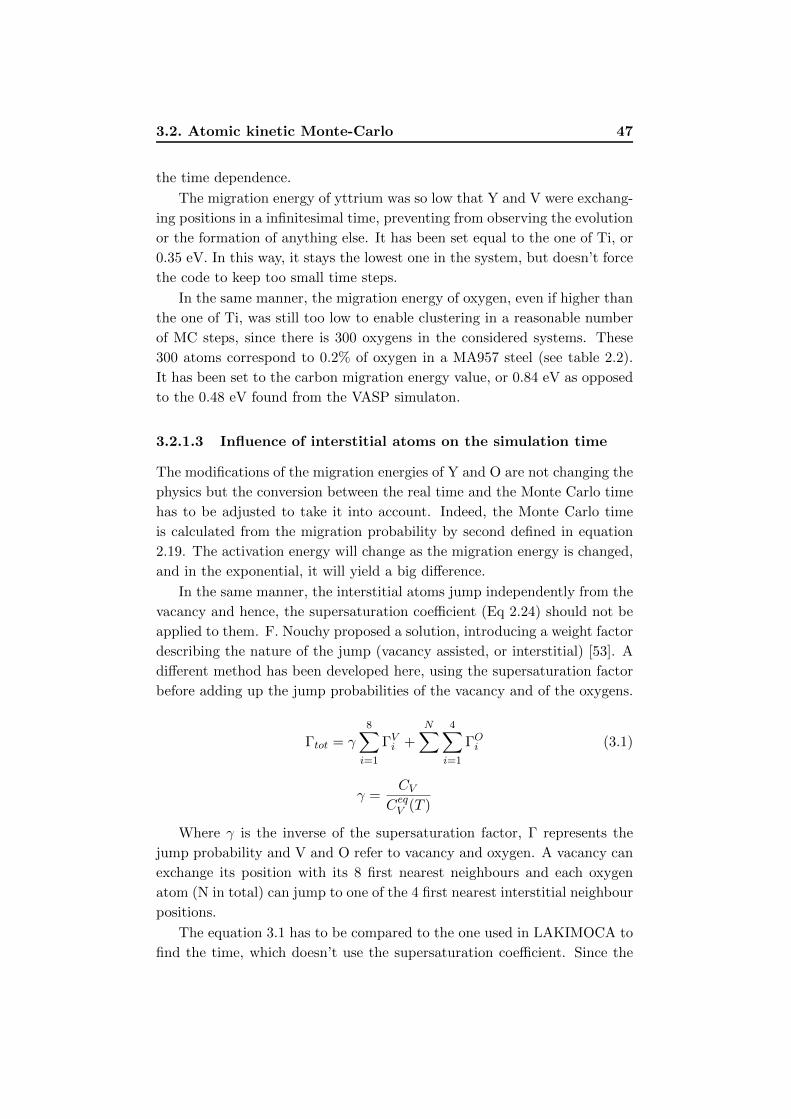
3.2. Atomic kinetic Monte-Carlo 47

the time dependence.

The migration energy of yttrium was so low that Y and V were exchang-

ing positions in a infinitesimal time, preventing from observing the evolution

or the formation of anything else. It has been set equal to the one of Ti, or

0.35 eV. In this way, it stays the lowest one in the system, but doesn’t force

the code to keep too small time steps.

In the same manner, the migration energy of oxygen, even if higher than

the one of Ti, was still too low to enable clustering in a reasonable number

of MC steps, since there is 300 oxygens in the considered systems. These

300 atoms correspond to 0.2% of oxygen in a MA957 steel (see table 2.2).

It has been set to the carbon migration energy value, or 0.84 eV as opposed

to the 0.48 eV found from the VASP simulaton.

3.2.1.3 Influence of interstitial atoms on the simulation time

The modifications of the migration energies of Y and O are not changing the

physics but the conversion between the real time and the Monte Carlo time

has to be adjusted to take it into account. Indeed, the Monte Carlo time

is calculated from the migration probability by second defined in equation

2.19. The activation energy will change as the migration energy is changed,

and in the exponential, it will yield a big difference.

In the same manner, the interstitial atoms jump independently from the

vacancy and hence, the supersaturation coefficient (Eq 2.24) should not be

applied to them. F. Nouchy proposed a solution, introducing a weight factor

describing the nature of the jump (vacancy assisted, or interstitial) [53]. A

different method has been developed here, using the supersaturation factor

before adding up the jump probabilities of the vacancy and of the oxygens.

Γtot = γ8∑i=1

ΓVi +N∑ 4∑

i=1

ΓOi (3.1)

γ =CV

CeqV (T )

Where γ is the inverse of the supersaturation factor, Γ represents the

jump probability and V and O refer to vacancy and oxygen. A vacancy can

exchange its position with its 8 first nearest neighbours and each oxygen

atom (N in total) can jump to one of the 4 first nearest interstitial neighbour

positions.

The equation 3.1 has to be compared to the one used in LAKIMOCA to

find the time, which doesn’t use the supersaturation coefficient. Since the

48 3. Results

jump probabilities have been changed as well, one has to find a new factor

to convert the MC time into the real time (Conv).

Conv =tMC

treal=

Γmodtot

ΓMC=

γ8∑i=1

ΓV,modi +N∑ 4∑

i=1ΓO,modi

8∑i=1

ΓVi +N∑ 4∑

i=1ΓOi

(3.2)

This equation can be simplified and expressed using the following vari-

ables.

X =

N∑ 4∑i=1

ΓOi

8∑i=1

ΓVi

(3.3)

where N is the number of interstitial oxygens, Γ represents the jump

probability.

Y =

N∑ 4∑i=1

ΓO,modi

N∑ 4∑i=1

ΓOi

= exp

(∆EmigkBT

)(3.4)

where N is the number of interstitial oxygens, Γ represents the jump

probability and the mod exponent designates the probability with the new

migration energy. ∆Emig is the difference between the modified and the old

migration energy values.

Z =

8∑i=1

ΓV,modi

8∑i=1

ΓVi

= 1− C + Cexp

(∆EmigkBT

)(3.5)

where Γ represents the jump probability and the mod exponent desig-

nates the probability with the new migration energy. ∆Emig is the difference

between the modified and the old migration energy values. C is the con-

centration of yttrium, or in a more general way, of solute whose migration

energy has been modified. C is the ratio between the number of Y and the

total number of atoms. C0 has been defined the same way for oxygen.

Finally, Conv can be expressed as

Conv =γZ +XY

1 +X(3.6)


Ideally, this coefficient should be calculated at every step of the MC

simulation. However, only a post simulation coefficient will be calculated

in this study. One has to be aware that for this reason, and others such

as vacancy trapping, abundantly discussed and illustrated by F. Nouchy

[53], this coefficient gives only an idea of the real time, and could not be

considered as more than a rough estimate.

γ can be calculated directly from the equation 2.25.

The other unknowns (X, Y and Z) has been calculated in average. For X,

the assumptions are that the matrix is pure iron except for the considered

defects. It means that both the vacancy and the O atoms are surrounded

only by Fe atoms. It also means that X depends only on the temperature

and on the number of oxygens.

In the same manner, Y and Z vary respectively with the temperature and

the temperature and the yttrium concentration.

The results are displayed in table 3.10. It can been seen that the con-

centration of yttrium has no or little influence on Conv. It can be explained

by the fact that a vacancy assisted jump is already less probable than an

oxygen jump, since there are so many more O atoms, whereas the concen-

tration of V is orders of magnitude higher than the supersaturation limit.

In addition to that, Y atoms represents only 0.2% of the total number of

substitutional atoms. It also explains that the γ factor has a limited effect

at these temperatures.

The main influence on Conv is, as expected, due to the O. Their jumps are

so likely that any change in their migration energy has a big effect.

Having a Conv bigger than 1 means that the real time is slower than the

MC time. It is the expected behaviour, since the mobility of several species

in the matrix has been reduced artificially. However, without interstitial

atoms, the supersaturation of vacancies is the predominant effect.

3.2.2 Formation of clusters

The goal here is to observe the formation of (Y,Ti,O) clusters in an iron

matrix containing 9% Cr, 1% Ti, 0.2% Y and 300 O (0.2%). To observe

which element has which effect, all of them has been added one by one

and the resulting clustering has been studied. In the pictures displaying

the results, neither Cr nor Fe are represented, as it would be impossible to

observe anything relevant if they were. Ti atoms are in red, Y atoms in

green, O atoms in blue and the vacancies in orange.

Firstly, since Y and Ti are believed not to cluster alone according to

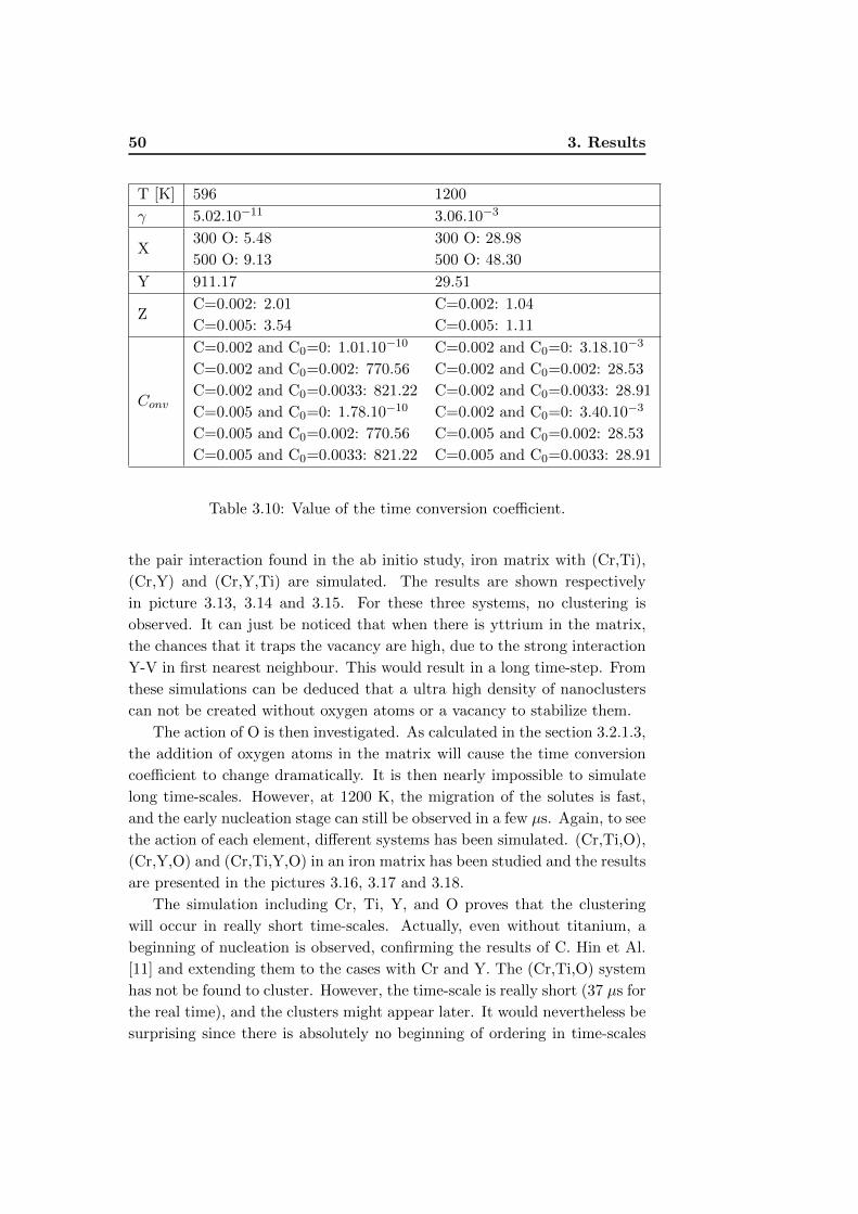
50 3. Results

T [K] 596 1200

γ 5.02.10−11 3.06.10−3

X300 O: 5.48

500 O: 9.13

300 O: 28.98

500 O: 48.30

Y 911.17 29.51

ZC=0.002: 2.01

C=0.005: 3.54

C=0.002: 1.04

C=0.005: 1.11

Conv

C=0.002 and C0=0: 1.01.10−10

C=0.002 and C0=0.002: 770.56

C=0.002 and C0=0.0033: 821.22

C=0.005 and C0=0: 1.78.10−10

C=0.005 and C0=0.002: 770.56

C=0.005 and C0=0.0033: 821.22

C=0.002 and C0=0: 3.18.10−3

C=0.002 and C0=0.002: 28.53

C=0.002 and C0=0.0033: 28.91

C=0.002 and C0=0: 3.40.10−3

C=0.005 and C0=0.002: 28.53

C=0.005 and C0=0.0033: 28.91

Table 3.10: Value of the time conversion coefficient.

the pair interaction found in the ab initio study, iron matrix with (Cr,Ti),

(Cr,Y) and (Cr,Y,Ti) are simulated. The results are shown respectively

in picture 3.13, 3.14 and 3.15. For these three systems, no clustering is

observed. It can just be noticed that when there is yttrium in the matrix,

the chances that it traps the vacancy are high, due to the strong interaction

Y-V in first nearest neighbour. This would result in a long time-step. From

these simulations can be deduced that a ultra high density of nanoclusters

can not be created without oxygen atoms or a vacancy to stabilize them.

The action of O is then investigated. As calculated in the section 3.2.1.3,

the addition of oxygen atoms in the matrix will cause the time conversion

coefficient to change dramatically. It is then nearly impossible to simulate

long time-scales. However, at 1200 K, the migration of the solutes is fast,

and the early nucleation stage can still be observed in a few µs. Again, to see

the action of each element, different systems has been simulated. (Cr,Ti,O),

(Cr,Y,O) and (Cr,Ti,Y,O) in an iron matrix has been studied and the results

are presented in the pictures 3.16, 3.17 and 3.18.

The simulation including Cr, Ti, Y, and O proves that the clustering

will occur in really short time-scales. Actually, even without titanium, a

beginning of nucleation is observed, confirming the results of C. Hin et Al.

[11] and extending them to the cases with Cr and Y. The (Cr,Ti,O) system

has not be found to cluster. However, the time-scale is really short (37 µs for

the real time), and the clusters might appear later. It would nevertheless be

surprising since there is absolutely no beginning of ordering in time-scales


Figure 3.13: System Cr-Ti at 1200 K after 2.9 seconds.

Figure 3.14: System Cr-Y at 1200 K after 98 days.

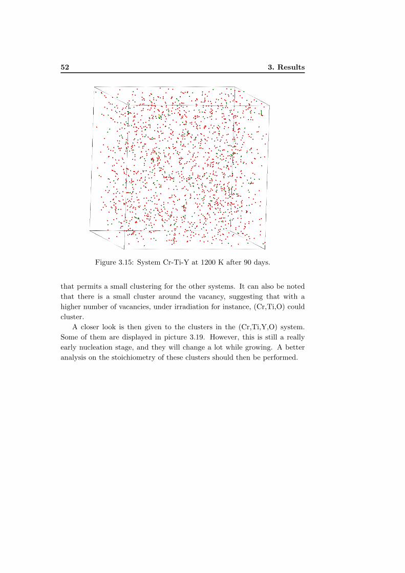
52 3. Results

Figure 3.15: System Cr-Ti-Y at 1200 K after 90 days.

that permits a small clustering for the other systems. It can also be noted

that there is a small cluster around the vacancy, suggesting that with a

higher number of vacancies, under irradiation for instance, (Cr,Ti,O) could

cluster.

A closer look is then given to the clusters in the (Cr,Ti,Y,O) system.

Some of them are displayed in picture 3.19. However, this is still a really

early nucleation stage, and they will change a lot while growing. A better

analysis on the stoichiometry of these clusters should then be performed.


Figure 3.16: System Cr-Ti-O at 1200 K after 37 µs.

Figure 3.17: System Cr-Y-O at 1200 K after 127 µs.

54 3. Results

Figure 3.18: System Cr-Ti-Y-O at 1200 K after 153 µs.

(a) Example of

cluster Y2T i2O

(b) Example of cluster Y T i2O3 (c) Example of cluster Y T iO3

Figure 3.19: Clusters at 1200 K after 153 µs.


3.2.3 Stability of clusters under normal conditions

In this part, the temperature has been set at 596 K. To test the stability

of the nanoclusters, several simulations have been made. Firstly, a Y2Ti03

cluster as found in the section 3.1.5, has been simulated alone with a vacancy,

then several of these clusters far apart in the simulation box, and finally a

much bigger cluster.

The new Conv coefficients for (2Y,3O) and (10Y,15O) has been calculated

using the formulas of the section 3.2.1.3 and are respectively 47.32 and 195.89

at 596 K.

For the simulation with just one cluster and one vacancy, it shows that

the vacancy finds the cluster and makes it more stable. After more than 12

minutes (real time), the cluster is still complete and shows no annunciating

sign of splitting.

The test on 5 clusters is even more conclusive. Even if the real time is

only around 2 seconds, the stability of the clusters has been observed without

a vacancy to stabilize the other four. One oxygen sometimes jump from one

cluster to another in a really short time. It is reasonable to assume that

this stability will last for much longer, but a new simulation is necessary to

prove it. However, due to the 15 oxygens in the system, the time conversion

coefficient is unfavorable and data for 60 years would be extremely long and

fastidious to acquire.

The same kind of behaviour is observed for the bigger cluster (5 times

the size of a Y2Ti03 cluster), also for around two seconds. The vacancy

finds the cluster and makes it more stable. Then an oxygen atom escape,

but it probably comes from the fact that this cluster is not in the optimal

geometric configuration.

56 3. Results

Chapter 4

Conclusions

This work is composed of two main parts. In the first one, the goal was to

find the binding energies of different defects in an iron lattice. This has been

done thanks to the DFT framework, using the Vienna Ab-initio Simulation

Package (VASP). In the second part, an atomistic kinetic Monte-Carlo code

has been used to help interpreting the results, and visualize the dynamics

of these defects.

In the part using first principles simulations, many basic geometric con-

figurations with chromium, titanium, yttrium and oxygen have been inves-

tigating and characterized as binding or repulsive. These results are valid at

0 K and within the limits of the approximations, which were the size of the

supercell, the sampling of the K points, the energy cut-off, the dilute limit,

and the approximations inherent in the DFT, for both the Hamiltonian and

the potential.

It has been shown that the chromium is not binding strongly with any

other considered defects (vacancy, Ti, Y, O). Concerning titanium, it is

respectively attractive and repulsive with a vacancy in first and in second

nearest neighbour. It also repels Cr and Ti but attracts O at short ranges.

Yttrium is bigger that the other atoms considered and will therefore bind

very strongly with a close vacancy. The special case with Y and a vacancy

in first nearest neighbour has been further investigated and the low diffusion

coefficient has been explained. An oxygen atom binds also really strongly a

vacancy at short ranges. It has been shown that a vacancy can actually bind

up to 6 oxygens. They also bind with titanium in 1NN and 2NN positions,

and with yttrium in 2NN position, whereas the 1NN one is strongly repulsive.

The interactions between two oxygens in octahedral positions have been

extensively studied, and it results from the calculations that two oxygens

are significantly binding only when they are one lattice parameter away and

58 4. Conclusions

without an iron atom between them.

From these raw data, the theoretical possibility of forming (Y,Ti,O) clus-

ters in the iron lattice have been discussed and proven. They can, according

to the experiments, be Y2TiO3 as well as Y2TiO5 and Y2Ti2O7.

The migration barriers of the different solutes have also been calculated,

and the very specific case of the yttrium has been discussed. It has been

concluded that the migration of an yttrium atom doesn’t depend on its

migration energy, but on the difference in binding with a vacancy in first

and second nearest neighbour.

Possible improvements of this part of the work could be to consider

always bigger supercells, with more K points and a higher energy cut-off. A

preliminary part of this study has nevertheless been based on finding optimal

parameters, combining reasonably converged results and fast calculations. It

could also be useful to continue the database on binding energies for n-tuples

instead of just for pairs. The influence of elements that are always in the

steel but in lower quantity, such as Ni, Mo or W, could also be investigated.

In the second part, these results have been used in an Atomistic Kinetic

Monte Carlo code (LAKIMOCA) to study the formation and the stability

of these clusters. The migration energies of Y and O have been increased

so they wouldn’t keep the time-step too small. The influence of this chnage

on the simulation time and on the real time has been quantified. This

quantification has only been applied after the simulations. For better results,

it is necessary to implement it into the code and to correct the time at each

step.

LAKIMOCA has also been vastly modified to improve the treatment of

the interstitial atoms. The temporal performances have not been deterio-

rated by more than 30 % after these changes.

The simulations have shown that clustering occur in the system thanks

to the oxygen effect. Indeed, Y and Ti can apparently not cluster by their

own. The chosen method has some major drawbacks: it considers that the

attraction between two defects in an otherwise perfect iron lattice stays the

same when the surrounding matrix is different. This has been briefly proven

wrong by adding a titanium atom close to a Y-V pair during the study of

the migration of yttrium. One other main issue is that this method doesn’t

allow a local change in lattice parameter or in crystal structure. When the

clusters are big enough, they should impose the crystallographic properties

locally. That is the reason why only the nucleation stage of the clusters can

be studied with an AKMC code. The limit of the nucleation stage is hard

to set, but the order of magnitude is a few tens of atoms.

The formation of nanoclusters at 1200 K has been proven, but only the

59

very early nucleation stage has been observed and the stoichiometry has

hence not been determined. The stability of these clusters at 596 K has also

been studied. Three different configurations have been investigated: one

Y2TiO3 cluster with a vacancy, 5 Y2TiO3 far apart with a vacancy, and a

bigger cluster of 30 atoms with the stoichiometry of Y2TiO3 and a vacancy.

All of them tend to prove that the clusters are stable for a significantly long

time.

The next step in this work is to study the stability of these clusters

under irradiation. However planned at first, this has not been done by lack

of time. It will necessitate further heavy modifications of LAKIMOCA to

improve the way the SIA are treated. The other major improvement of this

study would be to find a better way to handle the very likely events, so

that they don’t kill the simulations anymore by reducing the time-step too

much. It has been shown that the main problem in that matter is caused

by interstitial atoms, especially when their migration energy is low. This

would permit to have longer simulations, so presumably bigger clusters, and

then to study their stoichiometry and their size evolution.

60 4. Conclusions

Bibliography

[1] M. Klimiankou, R. Lindau, and A. Moslang. Energy-filtered TEM

imaging and EELS study of ODS particles and Argon-filled cavities

in ferritic-martensitc steels. Micron, 2005.

[2] S. Ukai, M. Harada, H. Okada, M. Inoue, and S. Nomura et al. Alloying

design of oxide dispersion strengthened ferritic steel for long life FBRs

core materials. J. Nucl. Mater., 204:74–80, 1993.

[3] S. Yamashita, S. Ohtsuka, N. Akasaka, S. Ukai, and S. Ohnuki. Forma-

tion of nanoscale complex oxide particles in mechanically alloyed ferritic

steel. Phylos. Mag. Lett., 84:525–529, 2004.

[4] Chu-Chun Fu and F. Willaime. Stability and Mobility of Mono- and

Di-Interstitials in α-Fe. Physical Review Letters, 92,17:175503, 2004.

[5] P. Olsson, C. Domain, and J. Wallenius. Ab initio study of Cr inter-

actions with point defects in bcc Fe. Physical Review B, 75:014110,

2007.

[6] Yong Jiang, John R. Smith, and G.R. Odette. Formation of Y-Ti-O

nanoclusters in nanostructured ferritic alloys: A first-principles study.

Physical Review B, 79:064103, 2009.

[7] D. Murali, B.K. Panigrahi, M.C. Valsakumar, Sharat Chandra, C.S.

Sundar, and Baldev Raj. The role of minor alloying elements on the

stability and dispersion of yttria nanoclusters in nanostructued ferritic

alloys: An ab initio study. Journal of Nuclear Materials, 403:113–116,

2010.

[8] C.L. Fu, Maja Krcmar, G.S. Painter, and Xing-Qiu Chen. Vacancy

Mechanism of High Oxygen Solubility and Nucleation of Stable Oxygen-

Enriched Clusters in Fe. Physical Review Letters, 99:225502, 2007.

62 BIBLIOGRAPHY

[9] D. Murali, B.K. Panigrahi, M.C. Valsakumar, and C.S. Sundar. Diffu-

sion of Y and Ti/Zr in bcc iron: A first principles study. Journal of

Nuclear Materials, 419:208–212, 2011.

[10] A.D. Le CLaire. Physical Chemistry: An Advanced Treatise, volume 10.

Academic Press, New York, 1970.

[11] C. Hin, B.D. Wirth, and J.B. Neaton. Formation of Y2O3 nanoclus-

ters in nanosctructured ferritic alloys during isothermal and anisother-

mal heat treatment: A kinetic monte carlo study. Physical Review B,

80:134118, 2009.

[12] C. Hin and B.D. Wirth. Formation of oxide nanoclusters in nanosc-

tructured ferritic alloys during anisothermal heat treatment: A kinetic

monte carlo study. Materials Science and Engineering A, 528:2056–

2061, 2011.

[13] W. Kohn. Nobel Lecture: Electronic structure of matter - wave func-

tions and density functionals.

[14] M. Born and R. Oppenheimer. Zur Quantentheorie der Molekeln. An-

nalen der Physik, 389,20:457–484, 1927.

[15] K. Burke. The ABC of DFT. Department of Chemistry, University of

California, 2007.

[16] P. Hohenberg and W. Kohn. Inhomogeneous Electron Gas. Physical

Review, 136:864–871, 1964.

[17] W. Kohn and L.J. Sham. Self-Consistent Equations Including Exchange

and Correlation Effects. Physical Review, 1340:1133–1138, 1965.

[18] N.M. Harrison. An Introduction to Density Functional Theory.

[19] W. Koch and M.C. Holthausen. A Chemist‘s Guide to Density Func-

tional Theory. Wiley-VCH Verlag GmbH, 2001.

[20] John P. Perdew, Kieron Burke, and Matthias Ernzerhof. General-

ized Gradient Approximation Made Simple. Physical Review Letters,

77,18:3865, 1996.

[21] Peter E. Blochl, Clemens J. Forst, and Johannes Schimpl. Projector

augmented wave method: ab initio molecular dynamics with full wave

functions. Bull. Mater. Sci., 26:33–41, 2003.

BIBLIOGRAPHY 63

[22] Peter E. Blochl, Johannes Kastner, and Clemens J. Forst. Electronic

structure method: Augmented Waves, Pseudopotentials and the Pro-

jector Augmented Wave Method. Handbook of Materials Modeling,

1:93–119, 2005.

[23] D. Vanderbilt. Soft self-consistent pseudopotentials in a generalized

eigenvalue formalism. Physical Review B, 41:7892–7895, 1990.

[24] M.L. McKee and M. Page. Reviews in Computational Chemistry, vol-

ume IV. VCH Publishers Inc., 1993.

[25] C.J. Cerjan and W.H. Miller. On finding transition states. J. Chem.

Phys., 75:2800, 1981.

[26] University of Texas. Nudged Elastic Band. http://theory.cm.

utexas.edu/vtsttools/neb/.

[27] Hannes Jonsson, Greg Mills, and Karsten W. Jacobsen. Nudged elastic

band method for finding minimum energy paths of transitions.

[28] George H. Vineyard. Frequency Factors and Isotope Effets in Solid

State Rate Processes. J. Phys. Chem. Solids, 3:121–127, 1957.

[29] P. Olsson. Modelling of Formation and Evolution of Defects and Pre-

cipitates in Fe-Cr Alloys of Reactor Relavance. PhD thesis, Uppsala

Universitet, 2005.

[30] M.S. Daw, S.M. Foiles, and M.I. Baskes. The embedded-atom method:

a review of theory and application, 1992.

[31] W.T. Read. Dislocations in crystals. McGraw-Hill, 1953.

[32] University of Kiel. Grain boundaries. http://www.tf.uni-kiel.de/

matwis/amat/def_en/kap_7/backbone/r7_1_1.html.

[33] G.H Kinchin and R.S. Pease. The Displacement of Atoms in Solids by

Radiation. Rep. Prod. Phys., 18, 1955.

[34] M.J. Norgett, M.T. Robinson, and I.M. Torrens. A proposed method of

calculating displacement dose rates. Nucl. Eng. Des., 33:50–54, 1975.

[35] G.R. Odette, M.J. Alinger, and B.D. Wirth. Recent Developments in

Irradiation-Resistant Steels.

[36] Janne Wallenius and Merja Pukari. Cladding materials and radiation

damage.

64 BIBLIOGRAPHY

[37] Stainless Steel 316 - Alloy Composition. http:

//www.espimetals.com/index.php/online-catalog/

202-stainless-steel-316-alloy-composition.

[38] M.L. Hamilton, D.S. Gelles, R.J. Lobsinger, M.M. Paxton, and W.F.

Brown. Fabrication Technology for ODS Alloy MA957, 2000.

[39] R. Lindauand A. Moslang, M. Rieth, and M. Klimiankou et Al. Present

development status of EUROFER and ODS-EUROFER for application

in blanket concepts. Fusion Engineering and Design, 75-79:989–996,

2005.

[40] A. Moslang. The development and characterization of EUROFER

ferritic-martensitic steel: the fusion perspective. In Nuclear Fission

& Fusion Steels Conference, 2009.

[41] F.A. Garner and H.R. Brager. The influence of Mo, P, C, Ti, Zr, Cr

and various trace elementson the neutron-induced swelling of aisi 316

stainless steel. Journal of Nuclear Materials, 155-157:833–837, 1988.

[42] F.A. Garner, M.B. Toloczko, and B.H. Sencer. Comparison of

swelling and irradiation creep behavior of fcc-austenitic and bcc-

ferritic/martensitic alloys at high neutron exposure. Journal of Nuclear

Materials, 276:123–142, 2000.

[43] S.I. Porollo, Yu.V. Konobeev, and S.V. Shulepin. Analysis of the be-

havior of 0Kh16N15M3BR steel BN-600 fuel-element cladding at high

burnup. Atomic Energy, 106-4:238–246, 2009.

[44] R.L.Klueh and D.J. Alexander. Embrittlement of 9Cr-1MoVNb and

12Cr-1MoVW steels irradiated in HFIR. Journal of Nuclear Materials,

187:60–69, 1992.

[45] K. Yagi and F. Abe. Long-term creep and rupture properties of heat

resisting steels and alloys. Acta Mettalurgica Sinica, 11,6:391–396, 1998.

[46] Y.T. Chiu and C.K. Lin. Effects of Nb and W additions on high-

temperature creep properties of ferritic stainless steels for solid oxide

fuel cell interconnect. Journal of Power Sources, 198:149–157, 2012.

[47] M.K. Miller, E.A. Kenik, K.F. Russell, L. Heatherly, D.T. Hoelzer, and

P.J. Maziasz. Atom probe tomography of nanoscale particles in ODS

ferritic alloys. Materials Science and Engineering A, 353:140–145, 2003.

BIBLIOGRAPHY 65

[48] H. Kishimoto, K. Yutani, R. Kasada, O. Hashitomi, and A. Kimura.

Heavy-ion irradiation effects on the morphology of complex oxide parti-

cles in oxide dispersion strengthened ferritic steels. Journal of Nuclear

Materials, 367-370:179–184, 2007.

[49] K. Yutani, H. Kishimoto, R. Kasada, and A. Kimura. Evaluation of

Helium effects on swelling behavior of oxide dispersion strengthened

ferritic steels under ion irradiation. Journal of Nuclear Materials, 367-

370:423–427, 2007.

[50] S. Jitsukawa, A. Kimura, A. Kohyama, R.L. Klueh, A.A Tavassoli,

B. van der Schaaf, G.R. Odette, J.W. Rensman, M. Victoria, and C. Pe-

tersen. Recent results of the reduced activation ferritic/martensitic steel

development. Journal of Nuclear Materials, 329-333:39–46, 2004.

[51] J.H. lee, R. Kasada, H.S. Cho, and A. Kimura. Irradiation-Induced

Hardening and Embrittlement of High-Cr ODS Ferritic Steels. Journal

of ASTM international, 6,8, 2008.

[52] P. Olsson, T.P.C. Klaver, and C. Domain. Ab initio study of solute

transition-metal interactions with point defects in bcc Fe. Physical

Review B, 81:054102, 2010.

[53] F. Nouchy. Monte Carlo Simulations for Thermal Ageing in Welding

Steels. Master’s thesis, Kungliga Tekniska Hogskolan, 2012.

ab initio based multi-scale simulations of oxide .../ab initio based multi... · ab initio based...

Documents