abdulbast mohamed elgwel a thesis submitted in … thesis_2013.pdfpossible to effectively count and...
TRANSCRIPT

ASPECT INDEPENDENT DETECTION AND
DISCRIMINATION OF CONCEALED METAL OBJECTS
BY ELECTROMAGNETIC PULSE INDUCTION:
A MODELLING APPROACH
Abdulbast Mohamed Elgwel
A thesis submitted in partial fulfilment of the
requirements of the Manchester Metropolitan University
for the degree of Doctor of Philosophy
School of Engineering
Division of Electrical and Electronic Engineering
Manchester Metropolitan University
2013
2
Abstract
The work presented in this thesis describes the research, modelling and experimentation
which were carried out so as to explore the use of electromagnetic pulse induction for the
detection of nearby or on-body threat items such as handguns and knives. Commercially
available finite difference time domain electromagnetic solver software, Vector
Fields, was used to simulate the interaction of a low frequency electromagnetic pulse
with different metal objects. The ability to discriminate between objects is based on
the lifetime of the induced currents in the object, typically around 100 (µs).
Lifetimes are different for a different objects, whether they are weapons or benign
objects. For example hand grenades, knives, and handguns are clearly threat objects
whereas a wrist watch, mobile phone and keys are considered benign.
Electromagnetic pulse Induction (EMI) relies on generating a time-changing but
spatially uniform magnetic field, which penetrates and encompasses a concealed
metallic object. The temporally changing magnetic field induces eddy currents in the
conducting object, which subsequently decay by dissipative (i.e. resistive) losses.
These currents decay exponentially with time and exhibit a characteristic time
constant (lifetime) which depends only upon the size, shape and material
composition of the object, whilst the orientation of the object is irrelevant. This
aspect independence of temporal current decay rates forms the basis of a potential
object detection and identification system. This thesis investigates the possibility of
detecting, resolving and identifying multiple objects if they are close together, for
example located on an individual. The mathematical analysis used for the
investigation implements the generalised pencil of function (GPOF) method. The
GPOF algorithm decomposes the signal into a discrete set of complex frequency
components; providing the capability to obtain the time constants from data. It was
possible to effectively count and identify multiple metallic objects carried in close
proximity providing that the objects do not have very similar time constants. The
simulation results, which show that multiple objects can be detected, resolved and
identified by means of their time constants even when they are close together, are
presented.

3
Acknowledgments
I would like to take this opportunity to express my sincere thanks and gratitude to
Professor Nicholas Bowring and Dr. Stuart Harmer for their continued patience,
inspiration, valuable guidance, advice, encouragement, and time.
They guided me through all the stages, giving valuable advice and encouraging me to
disseminate results in journals and so provided opportunities to communicate with
scientific researchers from different research institutions
I would like to thank to Shaofei Yin, member staff for his continuous support and
helping me to learn the simulation program also for the fruitful discussions.
I am also grateful to my mother and my family, especially my wife and my children;
they were the biggest motivation in completing my study.

4
List of Abbreviations
AMMW Active Millimetre Wave
CW Continuous Wave
CWD Concealed Weapon Detection
EM Electromagnetic
emf Electromotive Force
EMR Electromagnetic Resonance
EMW Electromagnetic waves
ELEKTRA/TR ELEKTRA transient
FDTD Finite Difference Time Domain
FEA Finite Element Analysis
FEM A finite Element Models
GPOF Generalised Pencil of Function
IED's Improvised Explosive Devices
INL Idaho National Laboratory
IR Infrared
MMW Millimetre Wave
NAC Nonlinear Acoustic
PMMW Passive Millimetre Wave
RCS Radar Cross Section
POF Pencil of Functions
RF Radio Frequency
SS Steady state
TR Transient
TDS Time Domain Spectra
THz Terahertz
WAMD Wide Area Metal Detection

5
List of Mathematical Symbols
A Cross Section Area
a Radius of Sphere (m)
B Magnetic Field (T)
D Electric field Displacement (C/m2)
E Electric Field Intensity (v/m)
Electromotive Force (v)
H Magnetic Intensity (A/m)
J Electric Current Density (A/m2)
L Inductance (H)
Mij Mutual Inductance
N Coil Turns Numbers
R Radius in Spherical Coordinates
0 Absolute Permeability ( H/m)
Conductivity (S/m)
Magnetic Flux (wb)
0 Fundamental Time Constant (ms)
Relative Permeability
0 Absolute Permittivity ( F/m)
Relative Permittivity
Skin Depth (m)
Electric Surface Charge Density (C/m2)
m Magnetic Susceptibility
n Solution of equation

6
Contents
Abstract ………………………….………………………………………..………... 2
Acknowledgments ……………………………………………………………………….…...3
List of Abbreviations ………………………………………………………………………....4
List of Mathematical Symbols …………………..……………………………….….……….5
Contents ………………………………………………………………………….…..………6
List of tables …………………………………………………………………..……………10
List of figures ………………………………………………………………...……………. 11
Chapter 1 .................................................................................................................. 14
GENERAL INTRODUCTION .......................................................................................... 14
1.1 Preview ........................................................................................................................ 14
1.2 Aim of project .............................................................................................................. 14
1.3 Objectives .................................................................................................................... 15
1.4 Organization of the Thesis ........................................................................................... 15
1.5 List of Publications Relevant to this Thesis .................................................................. 17
1.5.1 Peer Reviewed Journal Paper ................................................................................ 17
1.5.2 Conference Papers ................................................................................................ 17
1.6 Contribution to Knowledge .......................................................................................... 17
Chapter 2 .................................................................................................................. 19
Literature Survey ............................................................................................................... 19
2.1 Background .................................................................................................................. 19
2.2 Review of Current Concealed Objects Detection Research ......................................... 19
2.2.1 Metallic Objects Detection by Using Gradiometer ............................................... 20
2.2.2 Inductive Magnetic Fields ..................................................................................... 22
2.2.3 Acoustic and Ultrasonic Detection ....................................................................... 24
2.2.4 Target Recognition Using Electromagnetic Resonance ........................................ 26
2.2.5 Concealed Object Detection Using Millimetre Waves ......................................... 27

7
2.2.6 THz waves for concealed threat detection ............................................................ 30
2.2.7 Infrared Imaging ................................................................................................... 32
2.2.8 X-ray Imaging ....................................................................................................... 34
2.3 Discussion .................................................................................................................... 35
2.4 Summary ...................................................................................................................... 38
Chapter 3 .................................................................................................................. 41
Electromagnetic Induction concept .................................................................................... 41
3.1 Introduction .................................................................................................................. 41
3.2 Maxwell’s Equations ................................................................................................... 41
3.3 Boundary Conditions ................................................................................................... 44
3.4 Quasi-static Solution of Maxwell’s Equations ............................................................. 44
3.5 Electromagnetic Induction ........................................................................................... 45
3.5.1 Self Inductance ...................................................................................................... 46
3.5.2 Mutual Inductance ................................................................................................ 47
3.6 Skin Depth ................................................................................................................... 49
3.7 Summary ...................................................................................................................... 50
Chapter 4 .................................................................................................................. 51
Simulation Program and Building the Model .................................................................... 51
4.1 Introduction .................................................................................................................. 51
4.2 ELEKTRA Transient Mode ......................................................................................... 52
4.3 Model Great ................................................................................................................. 52
4.4 Defining Material Properties ........................................................................................ 52
4.5 Boundary of Model ...................................................................................................... 53
4.6 Mesh Size ..................................................................................................................... 54
4.7 Mesh Control ............................................................................................................... 54
4.8 Skin Depth and Meshing .............................................................................................. 55

8
4.9 Post Processing ............................................................................................................ 55
4.10 Simulation Program and Building the Model ............................................................ 56
4.11 Electromagnetic Theory for targets Detection and Identification .............................. 58
4.11.1 Time Constant for Sphere ................................................................................... 58
4.11.2 Mesh size calculation for Models ....................................................................... 61
4.11.3 Time Constant for Cylinder ................................................................................ 62
4.11.4 Time Constant of Simulation Models ................................................................. 64
4.12 Determination Time Constant of Sphere ................................................................... 66
4.12.1 Time Constant for Stainless steel Sphere ............................................................ 66
4.12.2 Time Constant for Titanium Sphere .................................................................... 67
4.12.3 Time Constant for Aluminium Sphere ................................................................ 68
4.12.4 Time Constant for Copper Sphere ...................................................................... 69
4.12.5 Time Constant for Two Spheres Together .......................................................... 70
4.13 Determination Time Constant for Cylinder ............................................................... 71
4.13.1 Time Constant for Stainless steel Cylinder ......................................................... 72
4.13.2 Time Constant for Titanium Cylinders ............................................................... 73
4.13.3 Time Constant for Aluminium Cylinder ............................................................. 74
4.13.4 Time Constant for Copper Cylinder .................................................................... 75
4.13.5 Time Constant for Two Cylinders Together ....................................................... 76
4.14 Summary .................................................................................................................... 77
Chapter 5 .................................................................................................................. 79
Using Electromagnetic Pulse Induction ............................................................................. 79
for the Detection of Concealed Metal Objects .................................................................. 79
5.1 Introduction .................................................................................................................. 79
5.2 Object Counting and Identification .............................................................................. 80
5.3 Time Constant of Threat Objects ................................................................................. 83

9
5.4 Time Constant of non-Threat Objects .......................................................................... 88
5.5 The Detection of Small Objects ................................................................................... 91
5.5.1 Sensitivity the of time constant to Key & Razor Blade ........................................ 91
5.5.2 Sensitivity of time constant to Key, Razor Blade & Wrist Watch ........................ 92
5.6 Resolution of Multiple Concealed Metallic Objects by Using Electromagnetic Pulse
Induction ............................................................................................................................ 93
5.7 Summary ...................................................................................................................... 96
Chapter 6 .................................................................................................................. 98
CONCLUSION AND FUTURE WORK .......................................................................... 98
6.1 Conclusion ................................................................................................................... 98
6.2 Future Work and Recommendation ........................................................................... 101
REFRENCES ......................................................................................................... 102
APPENDICES ........................................................................................................ 110

10
List of Tables
Table 2-1: The different techniques for detection concealed objects..................................... 37
Table 2-2: Main issues of the different techniques for detection concealed objects .............. 39
Table 4-1: Equation of time constant of sphere (modeling and theoretically) ....................... 66
Table 4-2: Stainless steel spheres for many radii ................................................................... 67
Table 4-3: Titanium spheres for different radii ...................................................................... 68
Table 4-4: Aluminium spheres with different radii............................................................... 69
Table 4-5; Copper spheres for two radii ................................................................................ 69
Table 4-6: Two stainless steel spheres (R=4cm and R=6cm) together .................................. 71
Table 4-7: Equation of time constant of cylinder (modelling and theoretically) ................... 71
Table 4-8: Stainless steel cylinders for many sizes ................................................................ 72
Table 4-9: Titanium cylinders for many sizes........................................................................ 73
Table 4-10: Aluminium cylinder............................................................................................ 74
Table 4-11: Copper cylinder .................................................................................................. 75
Table 4-12: Two stainless steel cylinders together ................................................................ 77
Table 5-1: Time constants of threat objects ........................................................................... 83
Table 5-2: Influence gun orientation on the time constant .................................................... 85
Table 5-3: Influence of knife orientation on the time constant .............................................. 86
Table 5-4: Groups of threat objects and the fundamental time constants. ............................. 88
Table 5-5: Time constant of representitive non-threat objects ............................................... 89
Table 5-6: A comparison of two, three objects together and the ........................................... 91
Table 5-7: Two small objects ( key & razor blade) ............................................................... 92
Table 5-8: Three small objects ( key, razor blade & wrist watch) ......................................... 93
Table 5-9: Groups of two to five objects and the fundamental time constants obtained from
these groupings; comparison with the Individual objects ...................................................... 95

11
List of Figures
Figure 2-1: Types of metal detectors ..................................................................................... 19
Figure 2-2: Gradiometer for detection metallic objects [4]. .................................................. 20
Figure 2-3: Magnetic gradiometer system (Bartington Instruments). .................................... 20
Figure 2-4: Principle of EMI technique for concealed metal detection [10]. ........................ 22
Figure 2-5: Metal detector with an object inside the detection space [2]. ............................. 22
Figure 2-6: Diagram of a 3D steerable magnetic field sensor system [10]. ........................... 23
Figure 2-7: Wide Area Metal Detector (WAMD) sensor system concept [12]. .................... 24
Figure 2-8: Crossed beam ultrasonic nonlinear acoustic generator for CWD [23]. ............... 25
Figure 2-9: Radar Cross Section is enhanced in the resonance region [25]. .......................... 27
Figure 2-10: Images resolution of the MMW system using 94 GHz [35]. ............................ 29
Figure 2-11: MMW images (imaging system) [36]. .............................................................. 29
Figure 2-12: Illumination of Fresnel optics with THz source from 3m [39]. ........................ 30
Figure 2-13: A range of threat and non-threat items imaged in the visible spectrum and at
640 GHz. The 640 Ghz image is on the right and and the visible image is shown on the left
[45]. ........................................................................................................................................ 31
Figure 2-14: 640 GHz image (left) of a toy gun under shirt. Visible image (right) [45]. ...... 32
Figure 2-15: Image of weapon concealed beneath a thin cotton shirt (left) and .................... 33
Figure 2-16: Image of weapon concealed beneath a thin cotton shirt (left) and .................... 33
Figure 2-17: Transmission of visible and IR radiation through the atmosphere [51]. ........... 34
Figure 2-18: Sample X-ray Images [55]. ............................................................................... 35
Figure 2-19: Electromagnetic spectrum and corresponding technologies. ............................ 36
Figure 3-1: Different types of magnetic material: Diamagnetic (a), ...................................... 43
Figure 3-2: (a,b): Electromagnetic induction - self-inductance circuits................................. 46
Figure 3-3 (a,b): Electromagnetic induction - Mutual-inductance circuits. ........................... 47
Figure 3-4: Types of metal detectors. .................................................................................... 49
Figure 4-1: (a) solenoid great with parameter, (b) Solenoid dimension. ............................... 52
Figure 4-2: (a) Model boundary, (b) Cross section of model boundary. ............................... 53

12
Figure 4-3: (a) Surface mesh parameter, (b) Volume mesh parameter, ................................. 55
Figure 4-4: Variation of magnetic field gradient with distance from the centre of coil......... 57
Figure 4-5: Simulation model – sphere between the transmitter coil and receiver coil. ........ 58
Figure 4-6: The magnetic fields caused by currents induced in the sphere. .......................... 59
Figure 4-7: The magnetic fields caused by currents induced in the cylinder. ........................ 62
Figure 4-8: Curve fitting of time constant for sphere. ........................................................... 65
Figure 4-9: Time constant for different radii of stainless steel spheres. ................................ 67
Figure 4-10: Time constant for different radii of titanium spheres. ....................................... 68
Figure 4-11: Time constant for different radii of aluminium spheres. ................................... 69
Figure 4-12: Time constant for different radii of copper spheres. ......................................... 70
Figure 4-13: Model of two stainless steel sphere (R=4cm and R=6cm). ............................... 70
Figure 4-14: Model of cylinder. ............................................................................................. 72
Figure 4-15: Time constant for stainless steel cylinder different sizes. ................................. 73
Figure 4-16: Time constant for titanium cylinder different sizes.......................................... 74
Figure 4-17: Time constant for aluminium cylinder. ............................................................. 75
Figure 4-18: Time constant for copper cylinder. ................................................................... 76
Figure 4-19: Model of two stainless steel cylinders .............................................................. 76
Figure 5-1: Flowchart depicting the processing steps and application .................................. 82
Figure 5-2: Four items of threat objects. ................................................................................ 83
Figure 5-3: Model diagram for gun, showing the size of the coils and positioning of the
threat item. ............................................................................................................................. 84
Figure 5-4: Time decays for hand gun, knife and razor blade. .............................................. 84
Figure 5-5: Time decay for hand grenade. ............................................................................. 84
Figure 5-6: Orientations of handgun. ..................................................................................... 85
Figure 5-7: Orientations of knife. .......................................................................................... 86
Figure 5-8: Model diagram for gun, knife and razor blade. ................................................... 87
Figure 5-9: Three items of non-threat objects. ....................................................................... 88
Figure 5-10: Model diagram for key. ..................................................................................... 89

13
Figure 5-11: Time decays for mobile phone, wrist watch and key. ....................................... 90
Figure 5-12: Model diagram for mobile phone, wrist watch and key. ................................... 90
Figure 5-13: Model diagram for key and razor blade. ........................................................... 92
Figure 5-14: Group of different metallic objects. .................................................................. 94

14
Chapter 1
GENERAL INTRODUCTION
1.1 Preview
Technologies for the detection of various concealed and buried metallic objects,
especially IED's (Improvised Explosive Devices), are currently of great topical
interest. Although there have been many studies, throughout the world, to curb and
prevent security threats in public places, such as concealed weapons and explosive
devices and buried ordnance (e.g. landmines) there is still no single sensor which
provides a complete solution to these problems.
Sensors capable of the detection of concealed, buried and hidden objects, both
metallic and non-metallic, which can also discriminate between threat items (suicide
vests, guns, knives, hand grenade and other deadly weapons) and non-threat items
(mobile phone handsets, jewellery and keys) would provide a very significant
enhancement of capability to security forces. These threats represent a considerable
challenge facing today’s law enforcement community [1]. In this field, the screening
techniques used for the detection of buried or concealed metal items are used in
banks, airports, public events and entrances of sensitive buildings, as well as at the
gates of prisons and courts. However such EMI devices cannot detect hidden objects
at any significant distance. To detect hidden objects they must be close to the
detection device in order to ensure sufficient sensitivity. According to the research
presented here, there is no device that can detect and identify concealed metallic
objects on the body with a high certainty of detection and identification and a low
probability of false alarms.
1.2 Aim of project
The aim of this project was to demonstrate the feasibility of detection and
identification of multiple conducting objects using EMI to excite circulating eddy
currents within the object. The results were realised by numerical simulation using a
finite element time domain electromagnetic solver that was capable of modelling

15
metallic objects of both threat and non-threat types. These objects were of different
shapes, sizes and materials. Modelling was carried out for singular objects; grouped
objects and in a variety of orientations and positions. The results were processed to
determine the fundamental time constant for these configurations of objects.
To detect and distinguish concealed metallic objects it is necessary to propagate
electromagnetic pulses to induce eddy currents to flow in the concealed or buried of
metallic objects. Analysis of the reflected (received) signals that take the form of
exponentially damped function field amplitudes provide the basis for the
determination of the time constant for the metallic object and thereby permits crude
identification of object type.
1.3 Objectives
The objectives of this research are to:
Design the modelling for several metallic objects of a range of representative
materials, threat and non-threat targets, by a Finite Element Simulation
program.
Find the fundamental time constants for many various shapes and sizes such
as spheres and cylinders, and other more representative objects separately and
with more than one object together, in various degrees of proximity.
Develop the electromagnetic pulse induction methodology to detect the
concealed and buried metallic targets in group and mix items together on the
body or in a bag.
Find and use a robust mathematical analysis technique generalised pencil of
function (GPOF) to analyse time decay(s) curves to reliably find the time
constants for targets, even when the targets are grouped together.
1.4 Organization of the Thesis
The thesis is organized as follows:
Chapter 1: General Introduction:
This chapter offers an overview of the project topic of the thesis and presents
the aims of the research, objectives, structure of the titles, novelty of research and
publication papers.

16
Chapter 2: literature survey
This chapter reviews and discusses many individual methods employed at
different frequency bands throughout the wide electromagnetic spectrum currently
used or that are the subject of research to detect concealed metal objects, describing
their advantages and disadvantages. Also, which of these methods are the most
widespread and common, include the devices that are used for this proposal.
Chapter 3: Electromagnetic Concepts
This chapter clarifies and explains the theoretical equations and methods
necessary to describe the concepts of electromagnetic induction by using Maxwell’s
equations and proves the mathematical steps that have been applied and describes the
solutions found during the course of this research, such as boundary conditions and
quasi-static solutions of Maxwell’s equations.
Chapter 4: Simulation Program
This chapter presents the development and building of FE models for a range
of objects such as spheres and cylinders, using several materials such as aluminium,
stainless steel, titanium and copper, , as isolated items and in proximity. Furthermore,
the methods for finding time decay(s) and for calculating the fundamental time
constant theoretical for these shapes and comprised with the simulated results.
Chapter 5: Using electromagnetic pulse induction (EMPI) for the detection of
concealed metal objects:
This chapter presents the main contribution to new knowledge and the novelty
of this research for using electromagnetic pulse induction at low frequencies to detect
concealed and buried metallic objects, both from threat and non-threat targets,
separately and mixed together as group (more than up to five items) on body or in a
bag.
Chapter 6: Conclusion and Future Work
6.1Conclusion: In this section explains and interprets the results and observations that
obtained from the simulation work and clarifies the features.
6.2 Future Work: This section presents the steps to the stage of the future and to
avoid mistakes and flaws also worthwhile proposals in order to provide adequate
solutions to detect these concealed targets.

17
1.5 List of Publications Relevant to this Thesis
1.5.1 Peer Reviewed Journal Paper
Abdulbast Elgwel, Stuart William Harmer, Nicholas Bowring & Shaofei Yin,
Resolution of Multiple Concealed Threat Objects using Electromagnetic Pulse
Induction, Progress In Electromagnetics Research, Vol. 26, 55- 68, 2012.
1.5.2 Conference Papers
1. Abdulbast Elgwel, Nicholas Bowring and Stuart Harmer, Detection of
Metallic Objects using Electromagnetic Pulses (Threat Targets), Research day
at Manchester Metropolitan University, 20th
April 2012.
2. Abdulbast Elgwel, Nicholas Bowring and Stuart Harmer, Electromagnetic
Pulses Induction for Detection of Metal Items (Non-threat Targets), Research
day at Manchester Metropolitan University, 25th
April 2013.
1.6 Contribution to Knowledge
The project presented in this thesis led to investigation of the the possibility of
detecting and identifying multiple concealed metal objects located on or about the
human body. Detection is by means of electromagnetic pulse induction at low
frequencies and the investigation is conducted using electromagnetic simulation tools.
Models are applied for many objects of different materials, shapes and sizes such as
spheres and cylinders also including easily carried weapons, for example a handgun,
hand grenade, razor blade and knife, and commonly carried benign objects, such as a
wrist watch, mobile phone and key. The materials simulated were (Aluminium,
copper, titanium and stainless steel).
In studying these phenomena we utilised a commercial finite difference time domain
electromagnetic solver software called vector fields. The model consists of a
transmitter coil that generates a primary magnetic field which induces eddy currents
to pass and flow on any concealed or buried metallic objects. The resulting
electromagnetic pulses (EMP) are induced in the receiver coil positioned some
distance away. The exponential decay rate of the induced current provides a time

18
constant, which depends upon the size, shape and the material from which the object
is made. The time constants are aspect independent, providing the basis for concealed
object identification.
The project demonstrated the ability to detect a number of objects and identify
multiple metal targets in close proximity. The results show that multiple objects can
be detected and identified even when the targets are close together.
19
Chapter 2
Literature Survey
2.1 Background
This chapter examines recent developments in the field of concealed and buried
metallic object detection. Many methods and means of utilising electromagnetic fields
have been applied to the problem of identifying concealed objects and especially to
determining whether the object detected constitutes a threat or not. Such methods
include: millimetre waves, x-ray, electromagnetic waves and infrared, and may be
passive or active in operation. There are devices available which are hand-held units
and also as walk-through (portal) units that are used for concealed weapon detection,
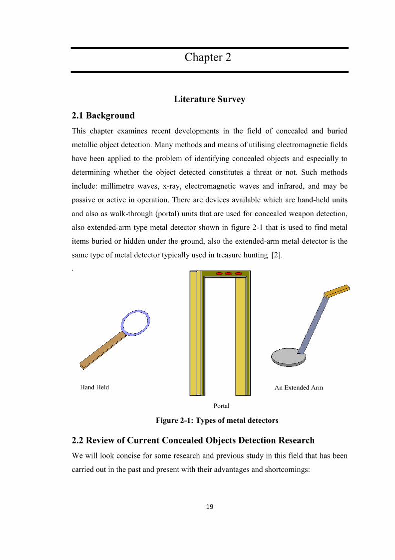
also extended-arm type metal detector shown in figure 2-1 that is used to find metal
items buried or hidden under the ground, also the extended-arm metal detector is the
same type of metal detector typically used in treasure hunting [2].
.
2.2 Review of Current Concealed Objects Detection Research
We will look concise for some research and previous study in this field that has been
carried out in the past and present with their advantages and shortcomings:
Hand Held
Portal
Walk Through
An Extended Arm
Figure 2-1: Types of metal detectors

20
2.2.1 Metallic Objects Detection by Using Gradiometer
This work is based on the principle of distortion in the Earth's magnetic field resulting
from ferromagnetic objects such as a hand grenade, handgun, razor blade and wrist
watch that are worn by people when passing through the portal see figure 2-2, or used
for locating objects buried in the ground, for example landmines and water pipes see
figure 2-3, also buried in the wall; for example pipe work and safes.. These types are
used in detection systems which are called Gradiometer metal detectors [3] see
figure2-2, the model contains two magnetometers connected by
electrical at differential mode to reduce the effects of background fluctuations that
would otherwise make false alarms. The gradiometer already responds to changes in
the magnetic field of the Earth from the moving ferromagnetic objects and based on
Figure 2-2: Gradiometer for detection metallic objects [4].
Figure 2-3: Magnetic gradiometer system (Bartington Instruments).

21
the magnitude of these interactions. The system can display the position of the metal
object through transit of the portal. This technology was developed like those in the
Idaho National Laboratory (INL), see Fig 2-2, which consists of 16 gradiometer
located on two sides of the portal system; the data is collected from each gradiometer
and the change in Earth’s magnetic field is calculated. In this way an image can be
generated which reveals the presence of metal objects being carried by the
person [5,6].
In figure 2-3 an idea has been implemented by Bartington Instruments [7] which
consists of two white cylinders that are the sensors that measure magnetic field
strength allowing a computer on the front of the harness to compute the gradient of
the Earth's magnetic field. The battery is mounted on the front under the computer.
This device is rather heavy. Other advanced electromagnetic techniques, such as a
magnetic real-time tracking vector gradiometer using high resolution fluxgate
magnetometers has been developed for incorporation into an unmanned underwater
vessel to improve mine detection. The unit comprises three primary three axis sensors
and one three-axis receive sensor [8].
The gradiometer for metal detection is considered a passive system because it requires
ferromagnetic objects; non-ferrous contraband objects such as explosives, electronic
batteries and non-ferrous metals like gold, Copper, Lead and Aluminium cannot be
detected. For this reason the system is not practical for most cases. Furthermore it is
deleteriously affected by vibration or movement induced errors that can cause false
alarm events. It may be possible to reduce the effects of motion and vibration using a
three-axis accelerometer to measure the change in the position of magnetometer and
therefore apply directed magnetic compensation for any vibration or movement, this
would clearly increase the additional circuit complexity and cost of the system.

22
2.2.2 Inductive Magnetic Fields
This unit used to control and detection in open area and indoor to find the objects
concealed at these areas, also used to detect hidden objects and contraband items in
the bags or on individuals and buried objects as landmines. Each user has different
security requirements, such as: airports, railway stations and courthouse security
require preventing entry of firearms and metal objects that can be used to injure the
people [9]. This technique uses active electromagnetic transmission to detect the
metal objects, sees figures (2-4, 2-5). Two coils are used, one is a transmitter coil
(source
Figure 2-4: Principle of EMI technique for concealed metal detection [10].
Figure 2-5: Metal detector with an object inside the detection space [2].

23
coil) and other is a receiver coil (detector coil). When current pulses with frequency
content around (5 KHz to 5 MHz) [10,11] flow in the transmitter coil producing a
time varying electromagnetic field around the coil that generates the primary
magnetic field and induces an electromotive force in the metal object causing eddy
currents to flow in the metal which generates the secondary magnetic field that can be
sensed by receiver coil. In figure 2-4 the target is located under the coils as in the
scenario for the detection of landmines. In figure 2-5 the target located between the
coils as may be the case in a walk through portal. In both examples the technique is
the same.
Wide Area Metal Detection [12,13] (WAMD) uses the method of pulse induction for
generating a time varying electromagnetic and relies on the time constants of the
induced eddy currents as a method of target identification. The sensors use a 3D
steerable magnetic field sensor [14] to generate and measure 3D time decay responses
of the magnetic field of the target see figure 2-6. WAMD works for any electrically
conductive or magnetisable objects, making this method a versatile system to scan for
prohibited objects. WAMD can also be used for screening in a crowded area, reducing
the need to screen for each person to be screened separately and without invading
individual privacy see figure 2-7.
Figure 2-6: Diagram of a 3D steerable magnetic field sensor system [10].

24
There are many techniques developed by a number of researchers, such as those
conducted at the University of Newcastle, using electromagnetic imaging techniques
for the detection and classification of threat and non-threat objects [15].
The inductive magnetic field method is not complete and still suffers a clear deficit in
the inability to detect low conductivity and non-conductivities materials and also
metal objects which are small in size. This difficulty arises because the signal
generated by the body is comparable to that generated by the small objects and then
the object passes undetected.
2.2.3 Acoustic and Ultrasonic Detection
The emission of acoustic waves with ultrasonic frequencies (> 20 kHz) into materials,
whether metallic or non-metallic, can be used to ascertain physical properties of
concealed objects. However the effects are dependent upon the shape, orientation, size
and hardness of material, also the diameter of the detector antenna, wavelength of the
acoustic signal emitted power [16] and it is therefore not a reliable method for
identifying objects concealed on the human body. The antenna size and wavelength
affect the minimum size of objects that can be detected on the body or buried in the
ground , for example landmines pipes or in investigation of both shallow and deep sub
bottom layers [17]. The sonic wave reflects from boundaries between materials with
different acoustical properties, and audio frequencies (low frequency) can be
Figure 2-7: Wide Area Metal Detector (WAMD) sensor system concept [12].

25
penetrate clothing or rough surfaces to detect and show hidden objects [18], while
ultrasonic detectors cannot penetrate thick clothing which makes it difficult to detect
concealed objects under such scenarios [19].
There are some hand held weapon detectors that work by emitting acoustic waves
and these systems generally function at ranges of 1m – 5m . JAYCOR advanced
Technology Company have developed a system which is a combination of radar and
ultrasound for producing ultrasound images and can operate at 5m-8m distance [19].
As shown in figure 2-8 [20,21] a nonlinear acoustic method (NAC) for CWD has
been developed which uses two sets of transducers to produce two ultrasonic beams
of differing frequencies, f1 and f2, to project sonic waves over long distances and
onto a small spot on the person. The ultrasonic frequencies are converted from
ultrasonic to audio frequencies by non-linear interactions which produce the
frequencies f1, f2, f1-f1, f1+f2. The difference, or beat frequency, frequency (f1-f2) is
chosen for detection and since the low frequency, i.e. audio frequency range, can
penetrate clothing and interact with the subject to detect concealed objects. Parametric
acoustic arrays can be used to produce nonlinear acoustic effects and the concealed
objects detection is dependent on acoustic signatures [22,23].
This technique is sensitive to solid objects and doesn’t inflict any harm on the body.
Ultrasound can also be used for holographic imaging to detect the concealed
objects [24], but some shortcomings are evident because there cannot be reliable
differential or discrimination between threat serious items and contraband and also
Figure 2-8: Crossed beam ultrasonic nonlinear acoustic generator for CWD [23].

26
between benign items. Thick, dense clothing such as leather causes high acoustic
reflection and targets concealed under it are difficult to detect.
2.2.4 Target Recognition Using Electromagnetic Resonance
Metal object detectors are used as instruments to search for dangerous or nuisance
metal objects that can be hidden in baggage, containers or on the body. These devices
are in some cases based on electromagnetic resonance (EMR) which utilise radar with
frequencies (200 MHz – 2 GHz). At these frequencies the Radar Cross Section (RCS)
varies in a rapid and oscillatory manner with frequency as is seen in Mie scattering.
The resonant response in the object is related to its physical size and composition but
is crucially also independent of the object’s orientation and is called a natural
resonance frequency that can be used to characterize the object [25]. The Resonance
based scattering exhibits some additional features that make it attractive for object
identification programs as follows:
The scattered is larger in the resonance region than it is below this region
(Rayleigh region).
The natural resonances are independent of the orientation of the object.
The resonance patterns of object uniquely identify the object. .
Several natural resonances can characterize an object over a large frequency
band.
The RCS depends on the ratio of wavelength to an object’s linear size [26] and the
RCS scattering falls in three regions which are termed Rayleigh, resonance (Mie) and
the optical region. The RCS of a sphere as function of its circumference, measured in
wavelengths, and normalized to the geometric cross section of the sphere can be seen
in figure 2-12. The resonance region of the sphere has many peaks that correspond to
the natural resonances of the sphere. When the circumference is large compared to a
wavelength, the oscillatory behaviour vanishes and the normalised RCS is now
independent of frequency and equal to the physical cross section of the sphere.
The target space is illuminated with either a pulse or swept frequency source and the
signal reflected by the objects in the target space provides an electromagnetic
signature for the objects [2]. The objects’ signatures are then compared to known
signatures to determine whether or not these objects are present in the target

27
space [27]. This technique is considered safe and low power, hence suitable for
human exposure, and also doesn’t invade the privacy of individuals.
In spite of, the EMR has good specifications of safety for human and can be
penetrates to away range for detection the concealed or hidden objects. However, the
EMR has some inabilities, as noise corresponding to the signature of people
contaminates the return signal. The signatures of people are different from person to
person; also the signature of person with any object such as weapon can be similar to
another person without weapon, potentially leading to false alarm high rates [28].
2.2.5 Concealed Object Detection Using Millimetre Waves
Millimetre wave (MMW) imaging, offers the possibility for remote screening of
persons for concealed metallic and non-metallic materials. Plastic explosives, drugs
and other contraband concealed under layers of clothing can be seen in many
circumstances when viewed in the millimetre-wave region of the electromagnetic
Figure 2-9: Radar Cross Section is enhanced in the resonance region [25].

28
spectrum. For the detection of concealed objects, the system is based on three major
factors: The apparatus is suitable in terms of over almost the entire millimetre-wave
region. The MMW region does not present health risks and observations can be made
remotely and with discretion as required. Active MMW systems emit very little
radiation; the emitted power is some ten thousand times smaller than that emitted by a
typical cell phone (the maximum rate (SAR) mobile standard for 2009 is
1.6 to 2 W/kg). MMW images are less physically revealing than x-ray images, and
this technology eliminates the problems with the use of ionizing radiation, as with x-
ray systems [29]. Millimetre waves can see through clothing and display the resulting
image, with a reduced capability of revealing intimate anatomical details, also MMW
systems have an enhanced standoff capability, when compared to x-ray imaging
scanners and as such can be used to scan crowds and be used in public places.
Furthermore, millimetre wave sensors measure the emission temperature through the
black body radiation that is emitted and (in the case of active systems) reflected from
the source that reflects from the target whether metallic such as weapons or grenades,
or non-metal, plastic explosives, bottles and other boxes [30,31].
There are two types of MMW screening systems, namely active and passive sensors.
Active sensors are by formed by generating and emitting signals that are focussed
onto the objects/target in question, interact with them and where signals are reflected
back to the sensor, because the self generated (emitted) signals have known properties
and often signal processing is used to enhance very weak emitted target signals from
noise sources, for example, when detecting landmines. For example, in the work of
Bosqetal, a novel active hyperspectral MMW scanning system was developed to
detect of buried landmines that used a vector network analyzer collecting the
backscattered MMW radiation from any buried objects
[32]. This method has
demonstrated an ability to detect metallic object buried under 3 inches of dry soil
[33]. The limitation of this method is that the emissions are usually weak.
Passive MMW sensors operating at 94 GHz and other wavelengths have been
reported [34]. Here, a set of receivers are spatially scanned over a target that form an
emissivity map, where objects concealed on the boy [35] show up because of differing
contrast, see figure 2-10. At microwave and millimetre wave frequencies surfaces
emit radiation that depends on parameters such as temperature and the amount of
emissivity. Metal surfaces have are strong reflectors of RF that masks the natural

29
emissivity and which produce reflections from other sources in the scene, with the
most significant being the sky. Figure 2-11 shows a passive MMW image formed
from the temperature differences emitted from the target or reflected from the source.
The output of the sensor is emissivity signals of objects in the MMW spectrum
and measure with receiver [36]. The MMW sensors can be penetrated clothing to
detect concealed metal objects due to low emissivity and high reflectivity of objects
such as metallic gun [28]. An imaging sensor working at 220 GHz has been
demonstrated for passive MMW imaging [37], which shows an acceptable image
quality for detection of metallic and non-metallic objects. At this relatively short
wavelength the MMW imaging is high resolution and clear for metallic and non-
metallic objects, the penetration of clothing is reasonably good, so the objects can be
visually detected. The detection ability of concealed objects is dependent on the
Figure 2-10: Images resolution of the MMW system using 94 GHz [35].
Figure 2-11: MMW images (imaging system) [36].

30
operating wavelength and the wavelength dependent on object properties (e.g. the
type of material and the size of the object). This system is basically FM diffraction
limited radar, with diffraction limiting the spatial resolution and consequent object
recognition. Developments of millimetre-wave systems for several years have led to
commercial MMW systems, mainly operating at 30 GHz, 94 GHz or 220 GHz,
designed for a range of checkpoint and stand-off people screening applications and
these are now beginning to become more widely used in this the field [38].
2.2.6 THz waves for concealed threat detection
Since the past several years, there has been an increased interest in the potential of the
technology for non-destructive and non-intrusive detection of concealed, buried
objects such as weapons, explosives, electronic cells, contraband also chemical,
biological agents and related devices. There are two methods to generate THz based
on optics and electronics. The optics method uses a single frequency far-infrared
laser, where THz wavelengths are generated by the mixing of two laser frequencies in
a photo conducting antenna, or using femto-second laser pulses (time domain
spectra TDS). These types of source are still at laboratory stage kind is developing,
see figure 2-12 [39-41]. The electronic method is by using electronic components, for
example superconductor-insulator-superconductor (SIS), Schottky-burrier diode
(SBD) hot electron bolometer HEB) mixer like heterodyne detectors [42]. There are
three techniques for generating THz using an electronic method, harmonic multipliers,
backward wave oscillators and quantum cascade lasers [43]. These types are now
readily available and are replacing the laser mixing or pulsed laser approaches.
Figure 2-12: Illumination of Fresnel optics with THz source from 3m [39].

31
Terahertz radiation can penetrate most non-metallic materials such as thin layers of
cloth, plastics and (partially), leather whereas metals completely block or reflect THz
waves. Thus, this technology can be used in imaging detection systems suitable for
the screening of personnel [44]. An example of sub-THz images taken at 640 GHz is
shown in figure 2-13. Here, a range of items are shown in pairs pairs, with the visible
image shown on the left and the 640 GHz image on the right.
So, when an object is carried on the body, whether metal or non-metal will show up as
an area of contrast on a THz image when compared to the body alone. The human
body has a high liquid content that will absorb nearly all T-Rays, with the energy
being harmless for the skin. Figure 2-14: shows an active THz image of a person
carrying a handgun, with the clothing appearing partially invisible and with a
reflection of the weapon, but the person’s skin appears substantially dark [45].
There are some barrier materials that mask concealed threats, with every material
having its own characteristic THz transmission spectra that must be taken into
account. The detection of land mines using THz waves imaging has some unique
considerations in terms of barrier materials, because the anti-personnel landmines are
small items and contain minimal amounts of metal and ground penetrating radar
systems, due to limited spatial resolution, cannot distinguish these small mines from
rocks [46,47].
Figure 2-13: A range of threat and non-threat items imaged in the visible
spectrum and at 640 GHz. The 640 Ghz image is on the right and and
the visible image is shown on the left [45].

32
THz waves have advantages of high resolution, the availability of a wide THz
spectrum and the use of a non-ionizing form of radiation to illuminate human
body [48]. However there are some drawbacks: THz has a limited output power when
using electronic methods of generation (e.g. harmonic multipliers) and they are
affected by the atmosphere, with strong absorbance at high frequencies [49]. They
are high cost, complex and require significant processing. Additionally, they require
special power sources, the scanning rate is slow (typically between 0.5 and 8 frames
per second) and the video output still poor. For the images shown here, the
wavelength close the infrared wavelength at femto-second laser as radiation
source [50].
2.2.7 Infrared Imaging
During the last couple of decades a considerable effort has been expended on
developing methods of detecting metal and non-metal objects concealed on a person
beneath clothing, in detecting contraband, devices or buried in the ground and walls,
these methods have included the use of infrared imaging technology. This technology
is primarily used for night vision applications and the principle of the theory is that
the infrared radiation emitted by the human body is absorbed by clothing after that re-
emitted. In figure 2-15 infrared radiation is used to show the image of a concealed
weapon with two clothing types, both a thin cotton shirt and a medium weight jacket.
Figure 2-14: 640 GHz image (left) of a toy gun under shirt. Visible image (right) [45].

33
In the case of a weapon concealed beneath cloth using a mid-wavelength infrared
between (3-5 micron) the image of concealed weapon is partly clear. In figure 2-16,
the wavelength has been lengthened to 8-12 micron consequently, the image of
concealed weapon will be clearer as they should penetrate fabric better. Normally, in
the cases of loose and thick clothing, the emitted infrared radiation will be diffused
over a large area, which reduces the ability to detect hidden objects [51].
The infrared radiation (IR) is generally transmissible through the air, can penetrate
through smoke and mist more readily than visible radiation. However, IR is affected
by atmospheric conditions such as rain or fog. So, IR is attenuated by the processes of
scattering and absorption, with IR and visible radiation exhibiting similar degrees of
attenuation, with gaps caused by absorption of various molecules, as shown in
Figure 2-15: Image of weapon concealed beneath a thin cotton shirt (left) and
a medium weight jacket (right) with mid wave (3-5 micron).
Figure 2-16: Image of weapon concealed beneath a thin cotton shirt (left) and
a medium weight jacket (right) with long wave (8-12 micron).

34
figure 2-17 [52]. IR can be used for detection of buried objects as the landmines and
pipes. This study relied on the soil thermal diffusivity and meteorological parameter
and the shape [53]. The difficulty in observing IR from concealed
objects becomes worse as the object temperature approaches that of the body, which
is likely to occur when the object is concealed on the body for a reasonable amount of
time, because the maximum contrast on an IR image is strongly dependent on the
temperature of the body and the object [54].
2.2.8 X-ray Imaging
The x-ray technology employed in these devices for detecting illicit hidden objects is
of low energy and penetrates few millimetres into body. Variants of the technology
are deployed for the inspection of items and baggage at security checkpoints in
airports [55]. This technique of x-ray differs from devices used in the medical field. In
the medical field, x-ray imaging relies on the absorption of incident x-rays for
imaging, whereas the x-ray system of concealed object detection relies on the
interaction of an x-ray photon with an electron bound to an atom and is called
Compton scattering or the backscattering effect/phenomena in quantum
mechanics [2]. This interaction occurs when an electron absorbs some of an x-ray’s
energy, whereas the absorbed energy is transferred to the kinetic energy that reduces
the energy of the x-ray photon interacting with an electron, with the scattered x-ray
photon used for imaging. X-ray imaging systems can provide high spatial resolution
to identify concealed and hidden objects on the body, within cases and containers and
Figure 2-17: Transmission of visible and IR radiation through the atmosphere [51].

35
in the ground, also its ability to penetrate clothing is high and, as such, the technique
can be usefully employed for the detection of metallic and non-metallic
objects [56,57], consequently weapons, explosives, chemicals, drugs, biological
agents, landmines and related devices can be found, see figure 2-18.
The x-ray system is sufficiently fast for high productivity applications, so within a
few seconds can make scans of person with high precision.
There are some shortcomings of using x-ray imaging, these x-ray systems emit low
dosages, however, there may be safety concerns surrounding ionizing x-ray radiation
and the United State Food and Drug Administration (USFDA) does not have an
official position on the safety of these devices. In addition when an examination the
person requires multiple scans, , furthermore it raises privacy issues.
2.3 Discussion
The literature survey has presented a limited study in the field of the detection of
concealed and buried objects, using different methods that are either deployed or
which are the subject of relevant research. The detection has to rely on the signal
responses from object picked by the sensors. However, many technologies are
currently employed for the detection of concealed objects. Many kinds of detection
sensors are in the process of being developed or are currently deployed, together with
many signal processing techniques which aim to improve the detection accuracy from
both an academic and an industrial aspect, including using the Gradiometer, inductive
the magnetic fields, acoustic and ultrasonic, millimetre waves, THz technology,
infrared imaging, x-ray imaging and electromagnetic resonance. The outline is
Figure 2-18: Sample X-ray Images [55].

36
illustrated in figure 2-19 to show EM spectrum used to detect the hidden objects by
the techniques described here.
The technologies described in this section form a summary of their lead purpose, their
deficiencies in performance in terms of vulnerability to weather factors, lights and
distance from the devices. Here they are summarised in terms of their performance
and the following definitions indicate to knowledge threat or contraband hidden
objects and ban it:
1. Detection: the discrimination process for targets of possible interest from their
environs.
2. Identification: determination of threat or contraband.
3. Classification: determination of the contraband or threat's characteristics.
Table 2-1 briefly refer to the techniques used in terms of their response to items as
well as its form and the energy used for interrogation at the detection distance, the
portability of the devices and proximity at which they operate.
Figure 2-19: Electromagnetic spectrum and corresponding technologies.

37
Table 2-1: The different techniques for detection concealed objects
No. The Technique Devices Signature Distance Portability
1. The Gradiometer Passive Near Transportable & Portable
2. Inductive the magnetic fields Active Near Transportable
3. Acoustic & ultrasonic detection Active Far Portable
4. Electromagnetic resonances Active Far Transportable
5. Millimetre waves Passive or Active Far Transportable & Portable
6. THz technology Active Near Transportable
7. Infrared imaging Passive Far Transportable
8. X-ray imaging Active Near Transportable
The Gradiometer is one device for the identification and detection of ferromagnetic
objects only; it has high ability for penetration and it is harmless passive
system. A challenge identified for Gradiometer is that it cannot detect non-
ferromagnetic objects and the Gradiometer is dependent on the distortion of the
earth’s magnetic field, which changes from day to night; this affects the sensitivity of
device. From a general review of papers, it can be assumed that the device is large,
expensive and costly. As for the inductive magnetic field type systems (i.e.
conventional metal detectors), these are active system with a high penetration ability,
but metallic objects only can be detected and identified; also the technique requires a
signature database to compare with a target. This technique has low sensitivity and
small size metal materials typically remain undetected when carried on the body.
With regard active acoustic technology, whether sonic or ultrasonic, these are
harmless, but detect rigid objects, including metal or non-metal. Furthermore the
technique suffers through a lack of penetration through many clothing types and it
does not distinguish between threat and non-threat items. The electromagnetic
resonance (EMR) is an active system safe for humans also it has penetration ability
from a short distance to detect concealed items, whether they be metal or non-metal
targets. However the EMR suffers from an inability to distinguish between threat or
benign equipment and tools, because the technique requires a signature database for
people which are different from person to person. Furthermore, EMR has a limited

38
ability to detect buried items in the ground such as landmines and distinguish between
them and, cans or pipes which can cause false alarms. The MMW technique is
commonly used for the detection of hidden objects or in the search for contraband and
more is an appropriate technology for deployment at airport security gates, as well as
in the detection and the search for buried land mines or pipe bombs. MMW systems,
whether they be active or passive, are portable or transportable by vehicle or movable
by hand. The MMW wave is not ionizing and consequently is harmless to the body
and it has high penetration ability for most clothing types. In some cases it can detect
both metallic and non-metallic objects. However, MMW detection is mostly based on
an imaging technology approach, and usually requires complex automated image
analysis software for object classification, making the system complex and costly.
THz technology can be used for active imaging systems, has high resolution and
detects metallic and non-metallic items. Such systems do, however, have some
drawbacks: it isn’t necessary capable of stand=off detection, is affected by the
atmosphere and THZ can be absorbed by the atmosphere at low frequencies
consequently the imaging quality produced is poor. Furthermore, the technology is
very expensive, making multiple pixel imagers very difficult to achieve. Infrared
imaging (IR) technology is a passive system and is known to be used at night to detect
both metallic and non-metals hidden targets. However IR imaging has low penetration
through all but very thin clothing and cannot differentiate objects at the same
temperature, furthermore IR is affected by atmospheric factors (e.g. rain, fog). X-rays
are active systems, with an ability to penetrate all clothing and baggage, and high
resolution. Similarly they also can detect metals and non-metallic objects. The
disadvantages are safety concerns for the body and a violation of privacy. The ability
to detect concealed threats at standoff distances is severely restricted.
2.4 Summary
Through this study of techniques and technologies, old and modern, which has
identified and briefly described a range of current detection methods, it can be
concluded that more research and development is required to overcome gaps in the
capability matrix. There is no technique that is fully capable of detecting hidden,
buried and concealed objects, without drawbacks. Table 2.2 identifies the main
capabilities of technologies that operate within the electromagnetic

39
spectrum Table 2-2: A summary of the techniques that have been described in this
Chapter, with their respective capabilities and the characteristics:
Table 2-2: Main issues of the different techniques for detection concealed objects
No. The Technique Devices Penetrable Objects Disadvantage
1. The Gradiometer High
Ferromagnetic
metallic targets
Non-ferromagnetic
targets undetectable
2. Inductive magnetic fields High Only metals
Location information
is lacking & not
enough sensitivity.
3. Acoustic & ultrasonic detection Medium Hard objects
Penetration deficient &
scanning deficient
4. Electromagnetic resonances High Metals & others
High false alarms &
needs a signature
database.
5. Millimetre waves High Metals & others
High cost & complex
system
6. THz technology Medium Metals & others
Lack of stand-off
detection capability,
can be absorbed &
expensive
7. Infrared imaging Low Metals & others
Low penetration,
affected by the
atmosphere and by
temperature
8. X-ray imaging High Metals & others
Safety concerns, &
privacy violation.
Lack of standoff
capablility.
All of these variant technologies are used in the detection of hidden or buried objects,
whether metal or non-metal, some of which presents an image and whereas others
produce different signals that denotes existence of an item. For instance, x-ray
imaging technology has the best results to show and detect concealed objects; it has a
high penetrative ability, produces an exceptionally clear image, it is the most modern
equipment suitable for the detection of hidden objects metals and others, but it has
implications for the health of the body and its users, as well as privacy issues. Also

40
studied and presented here are EM spectra alone or by combination (EM induction,
EM resonance and Gradiometer), which are complementary approaches to make an
improved system capable of operation in more circumstances.
The research presented in this thesis outlines a method of detecting concealed objects
using a variation of the commonly accepted method of Electromagnetic Pulse
Induction (EMPI). The variation on this existing method allows for the detection and
potential identification of multiple objects concealed in close proximity. The
identification of the concealed object enables classification algorithms to provide
information about it, for example if the object is considered as a threat or benign.

41
Chapter 3
Electromagnetic Induction concept
3.1 Introduction
The inductions of electromotive force by changing magnetic flux were first observed
by Faraday and by Henry in early nineteenth century from their pioneering
experiments have developed modern generators, transformers, etc. This chapter is
primarily concerned with the mathematical formulation of the law of electromagnetic
induction.
3.2 Maxwell’s Equations
Maxwell brought together a unifying set of equations which relate all
electromagnetic field quantities. These equations are usually written in vector
notation as
t
DJH (3.1)
t
BE (3.2)
D. (3.3)
0 B. (3.4)
where J (A/m2) is the electric current density and ρ (C/m
2) is the surface charge
density, E (V/m) is the electric field and B (T) is the magnetic induction, H (A/m) is
the magnetic intensity, D (C/m2) is the electric field displacement. Each of these
equations represents a generalization of certain experimental observations:
- Equation 3.1 represents is a time varying extension to Ampere’s law.
- Equation 3.2 is the differential form of Faraday’s law of electromagnetic induction.

42
- Equation 3.3 is the Gauss’s law for electricity, which in turn derives from
Coulomb’s law.
- Equation 3.4 is the Gauss’s law for magnetism, usually said to represent the fact that
single magnetic poles (monopoles) have never been observed, i.e. the net magnetic
flux entering any volume is zero, consequently a magnetic flux line is continuous;
there are no “sources” of magnetic flux.
The electromagnetic field is described by four field vectors; E, B, D and H. Then the
relationship between them are required to solve the electromagnetic field equation, the
electric displacement D is defined as
PED o (3.5)
Where is permittivity= 2
oo c/1 , and equals ( F/m). In the absence
of dielectric material, the polarization P=0. For the following work, it will be
assumed that all materials are non-polarisable, and thus the electric field and the
electric displacement are directly proportional
ED o (3.6)
The magnetic intensity H is defined to be related to B through the intrinsic
magnetization M is
)H(MBH
o
1 (3.7)
This equation M is explicitly written as a function of H. The magnetization vector M
is defined as the average magnetic moment per unit volume in the material or,
equivalently, the magnetic dipole polarization per unit volume.
For a non-magnetic material, such as copper, there is no magnetization (M=0) and
thus the magnetic intensity and the magnetic field density are related simply by
HB o (3.8)
The functional relationship of the magnetization with the magnetic field, M(H) helps
classify the three main classes of magnetic materials: diamagnetic, paramagnetic, and

43
ferromagnetic. The constitutive laws for the different magnetic materials are shown in
figure 3-1. In diamagnetic and paramagnetic materials the magnetization M and has
relationship with the magnetic intensity H and depend on the nature of magnetic
material. In large class of materials there exists an approximately linear relationship
between M and H, if the material is isotopic as well as linear.
HM m (3.9)
where m is the magnetic susceptibility at figure 3-1(a,b) and the magnetic
susceptibility of a diamagnetic material is negative
[58-60] and the magnetic
induction is weakened by the presence the material. The paramagnetic materials have
positive susceptibilities and the magnetic induction is strengthened by the presence the
material. In spite of m is function of the temperature and sometimes varies quite
drastically with temperature, it is generally safe to say that m for paramagnetic and
diamagnetic materials is quite small i.e ( 1m ).
Metals derived from iron or steel are ferrous metals. In ferromagnetic materials it is
more energetically favourable for the permanent magnetic moments throughout the
material to be aligned. This is in contrast to a dipole interaction; it is not energetically
favourable to have dipoles moments aligned. Throughout a ferromagnetic material
there exist domains in which all moments are aligned. The orientation of
b c a
Figure 3-1: Different types of magnetic material: Diamagnetic (a),
Paramagnetic (b) and ferromagnetic materials (c).

44
magnetization varies from domain to domain. When an external field is applied to the
material, domain walls move such that regions that are magnetized opposite to the
field are reduced in size.
3.3 Boundary Conditions
The boundary conditions that must be satisfied by the electric and magnetic fields at
an interface between two media are deduced from Maxwell’s equations exactly as in
the static case. The boundary condition applied to the magnetic induction from the
Maxwell’s equation as equation 3.4 [61]. Maxwell’s equations in differential form
describe the field at points where the divergence and curl of the fields exist. These
requirements thus exclude surfaces where Eand Hare discontinuous. Conditions on
the field vectors at the surface are derived by using the integral form of Maxwell’s
equations. The derivation of boundary conditions can be found in numerous texts
[62,63] and only the final results will be listed here. The normal component of the
electrical field is a discontinuous function at an interface that separates regions of
different conductivity and the normal component of magnetic flux density is a
continuous at an interface that separates regions of different magnetic permeability.
0).(ˆ
).(ˆ
21
21
BBn
DDno
(3.10)
where ρ is surface charge density. The tangential components of electric and magnetic
fields are continuous functions.
0)(ˆ
0)(ˆ
21
21
HHn
EEn
(3.11)
3.4 Quasi-static Solution of Maxwell’s Equations
When using Maxwell’s equations, the displacement current term tD in
equation 3.1 will be omitted. To establish the validity of this assumption we can
follow the steps [64]. The curl of equation 2.1 can be combined with equation 3.2 and
Ohm’s law EJ to give a dimensionless equation in E alone.

45
t
D JH
(3.12)
ED
0
t (3.13)
And (3.14)
Then the ratio is
1
t
J
D (3.15)
when applied Ohm’s law and equation (3.13), the equation (3.15) becomes
1 i 0
(3.16)
Where 2 , 1 , 12
0 1085.8 F/m, 610 S/m, and
2
2
0 a
where a=0.1 m, )m/H(104 7
0
,
Then the ratio of the coefficients (equation 3.16) is 13104.7 .
3.5 Electromagnetic Induction
In 1824, Oersted discovered that current passing though a coil created a magnetic
field capable of shifting a compass needle. After a few years, Faraday and Henry
discovered just the opposite. They have noticed a changing magnetic field would
induce current in closed circuit. This process of generating electrical current
in a conductor by placing the conductor in a changing magnetic field is called
electromagnetic induction or just induction. It is called induction because the current
is said to be induced in the conductor by the magnetic field. Induction is measured in
unit of Henries (H). When induction occurs in an electrical circuit and affects the flow
of electricity it is called inductance. The inductance is divided into two types.

46
3.5.1 Self Inductance
Any electric circuit which produces a magnetic field and it carries current, if the
current changes then the magnetic field will change and causing flux linkage with the
circuit [65] see figure 3-2 (a,b).
Thus for a rigid stationary circuit the only changes in flux result from changes in the
current. That is,
dt
d
d
d
dt
d I
I
(3.17)
Then ( Idd ) is a constant, equal to ( I ) and called the incremental inductance. In
any case, the inductance L is defined as
Id
dL
(3.18)
and
(3.19)
from equations (3.17), (3.18) and (3.19) it follows that the expression for the induced
electromotive force (emf)
(3.20)
where the electromotive force.
Figure 3-2: (a,b): Electromagnetic induction - self-inductance circuits.
(b) (a)
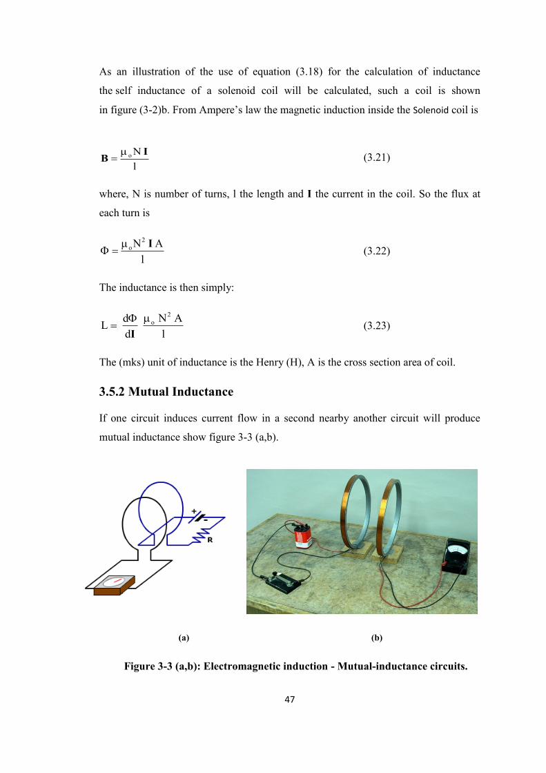
47
As an illustration of the use of equation (3.18) for the calculation of inductance
the self inductance of a solenoid coil will be calculated, such a coil is shown
in figure (3-2)b. From Ampere’s law the magnetic induction inside the Solenoid coil is
l
No IB
(3.21)
where, N is number of turns, l the length and I the current in the coil. So the flux at
each turn is
l
A N2
o I (3.22)
The inductance is then simply:
l
A N
d
d L
2
o
I (3.23)
The (mks) unit of inductance is the Henry (H), A is the cross section area of coil.
3.5.2 Mutual Inductance
If one circuit induces current flow in a second nearby another circuit will produce
mutual inductance show figure 3-3 (a,b).
(b) (a)
Figure 3-3 (a,b): Electromagnetic induction - Mutual-inductance circuits.

48
This restriction can be lifted by assuming that there are n circuits, labelled 1,2,3,…n.
The flux linking one of these circuits, say one labelled i, can be written
n
j
ijiniiii
1
321 ...................... (3.24)
The emf induced in the circuit can then be written as
n
1j
ijin1ii
dt
d
dt
d...............
dt
d
dt
d (3.25)
If each of the circuit is a stationary circuit, the only changes in the flux is that the
result from changes in the current, thus
dt
d
d
d
dt
d j
j
ijij I
I
(3.26)
The coefficients ( jij dd I ) are constants, independent of the current.
The mutual inductance between circuit I and circuit j is defined by
ji ,d
dM
j
ij
ij
I
(3.27)
The (mks) unit of mutual inductance are the Henries (H).
To calculate the magnetic induction for this situation that produces from first winding
l
N 11o IB
(3.28)
And consequently fluxes:
l
A N N
l
A N
1 21o21
1
2
1o11
I
I
(3.29)
From these fluxes the inductances can be became

49
l
A NL
2
1o1
(3.30)
l
A NL
2
1o1
(3.31)
From equation 3.18, then
l
A NNM 21o
21
(3.32)
Reversing the procedure and considering a current from another winding is
l
A 22
No2L
(3.33)
l
A NNM 21o
12
(3.34)
thus demonstrating that for this case M12 = M21. Furthermore the equations (3.21),
(3.22) and (3.23) may be combined to yield
2112 LLM (3.35)
3.6 Skin Depth
In discussion steady currents we noted that the current density was uniform over the
cross section of a cylindrical conductor show figure 3-4, if the source is oscillatory of
some frequency, then the current is pushed toward the surface of the conductor [66].
Figure 3-4: Types of metal detectors.

50
The eddy currents can only be carried between the outer surface and a level (layer) of
the metallic material, this phenomenon called skin depth ( ), and we simply state that
calculated by
f
1
0r (3.36)
where f is the frequency, is the conductivity of metal material, 0 is magnetic
permeability and. 1r . The SI unit of skin depth is meter (m) [67].
The skin effect due to effective resistance of the metallic materials also the skin depth
is low where high frequency and vice versa, i.e. the skin depth changes with
frequency and causing varies in the electrical field distribution on the surface layer.
Farther more the skin depth depends on the conductivity of the metal and vary
according the used the conductivity [68].
3.7 Summary
This chapter provided a concise review the electromagnetic induction that relates with
theoretical basic in this research and concept of the Maxwell’s equations and their
application and impact of this project. As well as to clarify aspects of the simulated
models to obtain on the good results and to avoid errors related to this project.

51
Chapter 4
Simulation Program and Building the Model
4.1 Introduction
The most important concepts for pre-processing, analysis and post-processing of
Opera-3d models are introduced. Building a geometry using the modeller, exploiting
the symmetry to reduce the size of model to be solved and generating the finite
element mesh are covered. Setting up the analysis by choosing appropriate material
characteristics, solution type and a solver module are also discussed. Finally, the Post-
Processor is used to obtain and present results from the analysis.
The simulation program is called Vector fields, version 13.0 - Opera-3d (an Operating
environment for Electromagnetic Research and Analysis) is the pre and post-
processing system for well known electromagnetic analysis programs including
TOSCA, ELEKTRA, SCALA, CARMEN, SOPRANO, DEMAG, QUENCH and
TEMPO.
Finite element discretization forms the basis of the methods used in these analysis
programs. This widely applicable technique for the solution of partial differential
equations requires special enhancements to make it applicable to electromagnetic field
calculations. Access to these features is supported by the Opera-3d Geometric
Modeller and pre-processor. These programs provide facilities for the creation of
finite element models, specification of complicated conductor geometry, definition of
material characteristics including, for example, nonlinear and anisotropic descriptions
and graphical displays for examination of the data.
Similarly, the Opera-3d Post-Processor provides facilities necessary for calculating
electromagnetic fields and displaying them as graphs and contour maps. The Opera-
3d Post-Processor can also calculate and display many derived quantities and can plot
charged particle trajectories through the calculated fields.
This work used the ELEKTRA Transient Mode to build the models simulate the
interacyion of electromagnetic fields with objects.

52
4.2 ELEKTRA Transient Mode
ELEKTRA Transient (ELEKTRA/TR) analyses time dependent electromagnetic
fields, including the effects of eddy currents, in three dimensions. There are three
analysis options: the time variation can be transient (TR), steady state ac (SS) or eddy
currents can be induced in moving conductors with a specified linear or rotational
velocity in the presence of a static field (VL). VL can be applied to situations where
the motion does not change the geometry, e.g. infinitely long rails or rotating disks.
4.3 Model Great
The Geometric Modeller provides facilities for creating models for use with the
Opera-3d analysis modules and Post-Processor. The Modeller manipulates any
defined objects through operations such as transformations and combinations. Basic
objects (blocks, cylinders, spheres, cones, pyramids and solenoids) can be created at
any position in space Special primitives can be defined in the Modeller to define
standard conductor shapes. These include racetrack coils, solenoids and others see
figure 4-1(a,b).
Figure 4-1: (a) solenoid great with parameter, (b) Solenoid dimension.
4.4 Defining Material Properties
The permeability of the magnetic materials will be defined using a nonlinear
characteristic curve. If the analysis is run linearly the initial slope of the curve will be
a b

53
used. If the analysis is run nonlinearly the curve will be used to match the
permeability of each element to the flux density. The materials will be treated as
isotropic. Material properties are assigned to material labels defined for each cell in
the model. In order for eddy currents to flow in the radiation shield electrical
conductivity must be defined.
4.5 Boundary of Model
Boundary conditions are used in two ways. Firstly they can provide a way of reducing
the size of the finite element representation of symmetrical models. Secondly they are
used to approximate the magnetic field at large distances from the model (far-field
boundaries). On individual far field surfaces a boundary condition is applied. Valid
boundary conditions are either relevant field components or perfect insulator.
Boundary condition BCRADIUS is associated with the curved surface of a cylinder or
sphere see figures 4-2(a,b).
One of the NORMAL or TANGENTIAL field conditions or the radiation condition
should be applied on all exterior boundaries and must be defined the sides of
boundary.
Figure 4-2: (a) Model boundary, (b) Cross section of model boundary.
The magnetic field must be determined in the free space that surrounds the magnet,
and this must also be included as part of the model. In the real world, this space
extends to infinity. In a finite element model though the free space region is
a b

54
terminated at a finite distance from the region of interest, such that the termination
does not significantly affect the accuracy.
4.6 Mesh Size
The final stage before creating a database and solving it is to create the model body
and mesh the model. The mesh generation of the finite element mesh is performed in
the Modeller and is a two stage process:
• Surfaces of models (cells) are initially meshed into triangles.
• Starting from the surface mesh, each cell is subdivided into a tetrahedral.
To prepare the model for meshing, the user must first execute the step model create
model body. This selects all entities as bodies, and performs a Boolean Union,
without regularisation. The result is one body with all cells retained.
4.7 Mesh Control
The element size can be controlled on vertices, edges, faces or cells within a model.
This allows the mesh to be refined in areas of interest where high accuracy is required
or where the field is changing rapidly. The element size can be controlled in several
ways [69]
• The Maximum element size is the maximum side length of an element. As each
cell is meshed it is high-lighted by its outline. Constructing the volume mesh takes a
few minutes and results in a mesh with about 280,000 elements and about 50,000
nodes,. These numbers of elements and nodes depend on the design and structure of
the model.
• The Maximum angle between elements defines the maximum angle between the
normal to adjacent elements on a curved surface.
• The Maximum deviation from surface defines the maximum distance between the
centroid of the planar surface element and the real curved surface it represents
see figure 4-3(a,b,c).

55
Figure 4-3: (a) Surface mesh parameter, (b) Volume mesh parameter,
(c) Model meshing.
4.8 Skin Depth and Meshing
The electromagnetic skin effect is the penetration depth of the field inside conductive
materials is dependent on the three parameters: electric conductivity, magnetic
permeability and frequency.
The skin/surface meshing is controlled by two considerations, the penetration depth
according to the perpendicular to the conductor, and the gradient of the state variable
according to the tangent. The meshing on the surface is related to the type of element,
and the skin meshing in boundary accurate check of the element sizes quadrangular
mesh form anisotropy, automatic meshing based on spatial distribution of the mesh
size. To fine layer elements, the material is modelled by its boundaries with boundary
finite elements on which particular boundary condition are introduced.
4.9 Post Processing
When the analysis has finished, the model starts running the solver, the database is
automatically activated and the results generated are stored. There are two ways in
which the model can be saved to file, first the model geometry and information on
materials and analysis settings can be saved in (an opc file) which can be read by
a b
c

56
edited by the Modeller, second and analysis database (an op3 file) must be saved for
ELEKTRA/TR to analyse.
This chapter presents the software and the simulation models used to investigate the
electromagnetic induction using cylinders and spherical models of varying
dimensions and materials including copper, titanium, aluminium, and stainless steel.
In addition, a comparison between the theoretical and simulation results is presented.
4.10 Simulation Program and Building the Model
Numerical simulation is carried out using the commercially available finite element,
time domain, electromagnetic solver software from Vector Fields. The first issue that
is addressed in modelling of the various EMI scenarios is that of specifying the
external magnetic field. This field should be spatially uniform over a sufficient
volume that the modelled objects can be moved within this volume without unwanted
effects from spatial magnetic field gradients across the objects. The effect of a
spatially varying magnetic field across the object would be to introduce a degree of
aspect dependence to the time constants and thus degrade the property of aspect
independence upon which the method relies. A large, circular coil is suitable for the
purpose of generating a spatially uniform field. The magnetic field is uniform over
distances that are commensurate to typical concealed metallic objects such as weapon
sizes (~20 cm) providing the coil is much larger than this size. Accordingly, a coil 4
metres in diameter was chosen as being suitable for this purpose and called
transmitter coil that can transmit step pulse of current causing eddy currents to flow
and excited in target metal object. The eddy currents scatter a signal that will be
detected by a receiver coil. The receiver coil is 2 metres in diameter that receives the
signal after being reflected from the object and take exponential form of decaying
transient at the same time following sudden changes in the magnetic field. Yet not so
large as to render computation time excessive on a standard PC. It should be stated
that this choice of magnetic field source may very well be suboptimal when
consideration is given to the design of a practicably deployable device. In this case,
several smaller coils may be arranged to give a plane where the magnetic field is
uniform or long parallel wires carrying current may instead be used to achieve
uniformity of field in the desired sensing region.

57
In order to study the effect that varying object separation has on the ability to detect
and discriminate objects within close proximity using EMI it is necessary to be able to
alter the position of the various objects within the coil, without moving the object(s)
into a region where there is significant magnetic field gradient see Figure 4-4.
A graph illustrating the calculated magnitude of magnetic field gradient, expressed as
a percentage (i.e. % change per metre), from a 4 metre diameter coil as a function of
distance from the coil centre and distance from the plane of the coil. The magnetic
field strength is normalised by the axial field magnetic strength in the plane of the
coil, evaluated at the coils centre.
In fact the 4 metre diameter coil provides a very uniform magnetic field over a
considerable region around the coil centre; see Figure 4-5. The axial and radial field
components are normalised by to the axial component of the magnetic field, in plane
and at the coil centre. The central region of the coil, extending one metre from the
centre and one metre from the plane of the coil, has a normalised magnetic field
gradient which is less than 2.5% per metre giving a maximum change of ~ 0.5% for a
20 cm sized object. This value is more than adequate for this EMI application;
therefore we may move our objects within a ~3 m3
cylindrical volume located at the
centre of the coil without encountering problems.
Figure 4-4: Variation of magnetic field gradient with distance from the centre of coil.

58
The finite time domain solver creates a mesh (of finite elements) on which Maxwell’s
equations is solved, the mesh must have an element size which is sufficiently small to
resolve the interaction of the electromagnetic fields within the conductor. The scale of
the mesh size required can be judged by computing the skin depth of the metal
conductors from which the objects are being modelled.
4.11 Electromagnetic Theory for targets Detection and Identification
There is published work in the field of EMI for a variety of uses, concealed metallic
objects detection; ground penetrating radar for unexploded ordnance detection and
mining. These applications rely on the same phenomena and share a common
theoretical underpinning.
4.11.1 Time Constant for Sphere
In studying the electromagnetic induction for regular shape sphere in the three axes
show figure 4-6 the expression for the vector potential outside sphere is [70-73]
1s
22
s
tq23
z0
e
)]2K)(1K(a [
e sinR a B K3A
s
(4.1)
Figure 4-5: Simulation model – sphere between the transmitter coil and receiver coil.

59
The quantities of equations are defined as follows:
2
0
22
0
2
ss
a
s
q
(4.2)
a
s s
where, s = 1,2,3,….. (4.3)
2
1K
(4.4)
‘‘t’’ is a time of initiation of the current step, and R is the radius in spherical
coordinates.
AB
t
AE
(4.5)
By using quasi-static solution of Maxwell’s equations, the primary magnetic field
around the sphere increases by amount due to currents induced flowing through the
sphere and after applied equation 4.5 over equation 4.1, and then can obtain the
following expression for three axes of the fields:
1s
22
s
tq
s23
z0
e
)]2K)(1K(a [
eq sinR a B K3E
s
(4.6)
Figure 4-6: The magnetic fields caused by currents induced in the sphere.
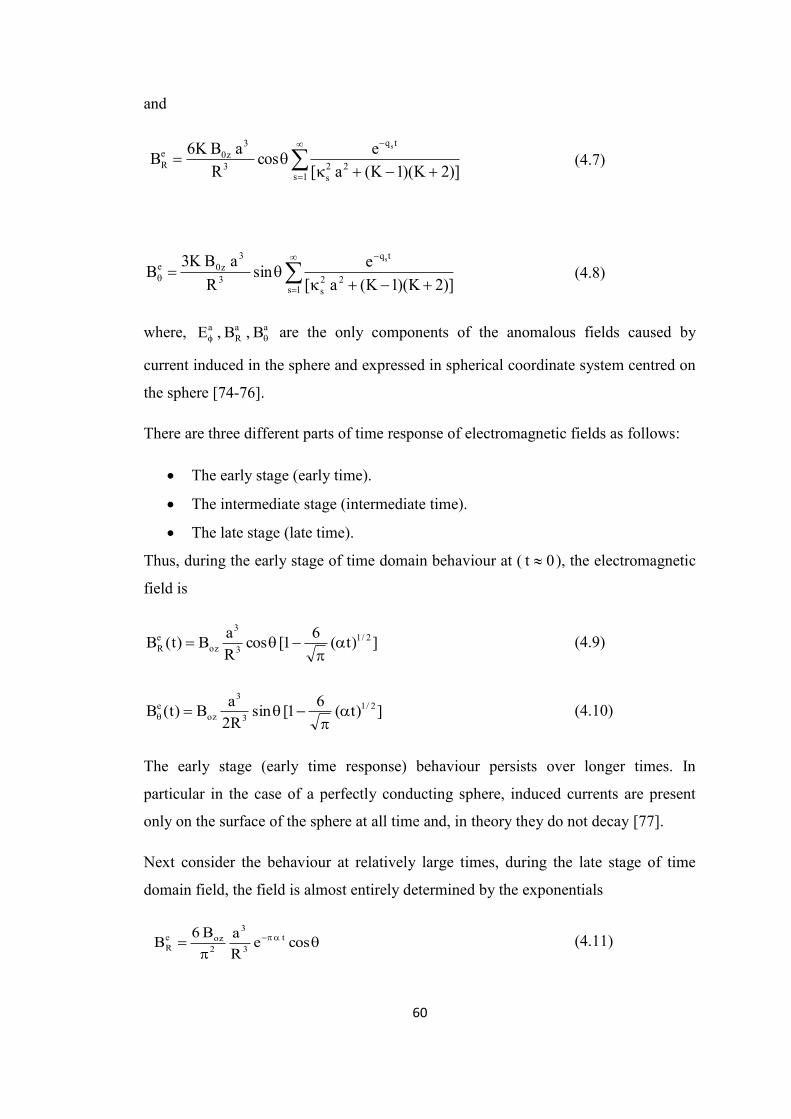
60
and
1s22
s
tq
3
3
z0e
R)]2K)(1K(a [
e cos
R
a B K6B
s
(4.7)
1s
22
s
tq
3
3
z0e
)]2K)(1K(a [
e sin
R
a B K3B
s
(4.8)
where, aa
R
a B , B , E are the only components of the anomalous fields caused by
current induced in the sphere and expressed in spherical coordinate system centred on
the sphere [74-76].
There are three different parts of time response of electromagnetic fields as follows:
The early stage (early time).
The intermediate stage (intermediate time).
The late stage (late time).
Thus, during the early stage of time domain behaviour at ( 0t ), the electromagnetic
field is
])t( 6
1[ cos R
a B)t(B 2/1
3
3
oz
e
R
(4.9)
])t( 6
1[ sin R2
a B)t(B 2/1
3
3
oz
e
(4.10)
The early stage (early time response) behaviour persists over longer times. In
particular in the case of a perfectly conducting sphere, induced currents are present
only on the surface of the sphere at all time and, in theory they do not decay [77].
Next consider the behaviour at relatively large times, during the late stage of time
domain field, the field is almost entirely determined by the exponentials
cose R
a
B 6B t
3
3
2
oze
R (4.11)

61
sine R
a
B 3B t
3
3
2
oze (4.12)
sine a R
B 3B t 3
2
oze (4.13)
The late time is defined by inequality
2
1t (4.14)
Then, the late time for transient field will be observed and the components of the
electromagnetic field and can be written as
0/t
3
3
2
oze
R e cos R
a
B 6B
(4.15)
0/t
3
3
2
oze e sin R
a
B 3B
(4.16)
0/t
2
3
2
0
oze e sin R
a
B 3B
(4.17)
The parameter 2
1 is called the time constant 0 for the spherical conductor, and
2
0 a
1
,, hence
2
2
0
20
a
1
(4.18)
where, 0 is absolute permeability of free space and equals ( H/m), is
conductivity and a is radius of sphere.
The equation (4.18) is important for determine the time constant theoretically for the
sphere and already applied in these results.
4.11.2 Mesh size calculation for Models
The maximum mesh size required is
, , where might typically be 10 (i.e. 10 is
target maximum mesh element size at generate surface mesh in the model). The

62
electromagnetic frequency can be well estimated by taking the reciprocal of the
fundamental time constant for a sphere, also with Equation (3.36), where r = 1.
Substituting this into Equation (4.18) gives the expression and the typical frequency
constant of decaying electromagnetic field:
2
0
2
0 a
1f
(4.19)
and topical λ of decaying in the vacuum:
2
2
0 a c
f
c
(4.20)
then the topical skin depth in object is:
23
a
(4.21)
For example the typical object in (a = 0.1 m) and conductivity ( 176 m.S1010 )
the skin depth can be calculated from equation (4.21) as
cm8.10.1
23
4.11.3 Time Constant for Cylinder
To study the electromagnetic induction for regular shape solid cylinder in the three
axes show figure 4-7 the equation of the vector potential is:
Figure 4-7: The magnetic fields caused by currents induced in the cylinder.

63
For using quasi-static solution of Maxwell’s equations, the magnetic field flows
through the cylinder and produces the eddy currents around the cylinder, the step
response function in time domain is [78]
12
rr
tS
r
r
r3 )t(u)()1)(2(
e6
)2(
)1( 2a 2)t(s (4.22)
In terms of the positive real decay time constants
S
1 (4.23)
and the roots of the transcendental equation given the time constants:
2
0
2
)(
a
(4.24)
the magnetic polarizability is derived
12
0rr
/t
r3 )t(ua )1)(2(
e6)t(a 2)t(M (4.25)
where )t( is dirac delta function and )t(u is step function, and by a Fourier or
Laplace transform could be taken to give the relative permeability of the shape as
function of frequency to find the roots. These roots would give the magnetic
polarizability in frequency domain, then the equation becomes [78]:
)t(u n
e a 50)t( s
1n22
/t3
0
(4.26)
with
18
h a 0
0
(4.27)
where, h is height of cylinder. The equation (4.27) is time constant for solid cylinder.

64
4.11.4 Time Constant of Simulation Models
The time constant can also be determined from the models by using simulation
program for any metallic objects. The time domain dependence of the induced voltage
on the secondary of the receiver coil can be expressed [79-81] as
nn
n
texpA)t()t(V (4.28)
where nA and n are the amplitudes and time constants respectively, of the nth
eddy
current mode circulating in the object. In general, an analytic solution giving the
values of nA and n is not possible for all, but a few very simple cases where
symmetry allows for an analytical expression. A conducting sphere is one such
case [82,83]. For a sphere of radius R; conductivity and relative permeabilityr ,
the time constants n are given by
2
n
2
0rn
R
(4.29)
where n are the solutions of the equation
2
n
nn
1
)1()tan(
(4.30)
The time dependence given by Equation (4.23) simplifies further for times which are
long, when compared to the time constants of the higher (n ≥ 2) order modes. In this
late time regime, after the excitation pulse or the switching off of the current in the
primary coil that provides the spatially uniform magnetic field, the voltage induced in
the secondary coil is simply
1
texpA)t(V (4.31)
Thus we may identify an object by its aspect independent, fundamental time constant
which is dependent only upon the shape, size and material that form the object.

65
-2 -1.5 -1 -0.5 0 0.5 1 1.5 2 2.5-6
-4
-2
0
2
4
6x 10
-4
Time - ms
Vo
ltag
e -
v
v,t
fit 1
When M multiple objects are present within the magnetic field the detected signal,
again for times which are long compared to high order modes, will simply be the
superposition of the signals for the objects individually,
M
1n 0
n
texpA)t(V (4.32)
And equation (4.32) can be written
M
1n
n )btexp(A)t(V (4.33)
Where 0
1b
, i.e b is the quantity that obtained from fitting curve by MATLAB.
The results obtained are processed with MATLAB program (non-linear fitting
algorithms) for calculation the time constant, and the fitting curve applied to sphere is
shown in figure 4-8 and an exponential decay curve appears as straight line with slop
being the time constant. The slop of line (time constant) is extracted by curve fitting
of transformed data.
Figure 4-8: Curve fitting of time constant for sphere.

66
4.12 Determination Time Constant of Sphere
In this section calculate time constant for sphere theoretically and from the simulation
models shows table 4-1 below. The expression shows the potential of using the time
constant in identifying a many spheres for different radii and many materials
(Stainless steel, Titanium, Aluminium and Copper). All spheres of different materials
and the same radii will be characterised by a scattered electromagnetic field and time
constant will be different. Thus the spheres can be classified, at least within the
precision with which the time constant of the decaying magnetic field can be
determined.
Table 4-1: Equation of time constant of sphere (modeling and theoretically)
Time constant from Simulation
(s) 0
Time constant from Theoretical equation
(s) 0
)t
exp(- A)(0
n
tV 2
2
00
a
4.12.1 Time Constant for Stainless steel Sphere
Numerical simulation is carried out using the commercially available finite element,
time domain. A large, circular coil is suitable for the purpose of generating a spatially
uniform field over distances that are commensurate to all sizes and shapes.
The model was validated by simulation of stainless steel spheres of conductivity
1.1×10⁶ S.m
-1 and of different radii. The fundamental time constants from the
simulations were compared to theoretical equation and the simulated results agree
well with theory, see Table 4-2, and time decays are appeared clearly in the figure 4-9

67
0 0.5 1 1.5 2 2.50
1
2
3
4
5
6x 10
-4
Time - ms
vo
lta
ge
- v
R=3cm
R=4cm
R=5cm
R=6cm
Table 4-2: Stainless steel spheres for many radii
Material Radius Simulation (ms) lTheoretica (ms)
Stainless Steel
3.0 cm 0.1212 0.1260
4.0 cm 0.2212 0.2241
5.0 cm 0.3502 0.3501
6.0 cm 0.5068 0.5042
4.12.2 Time Constant for Titanium Sphere
Variations of the simulation and theoretical time constants for titanium spheres of
conductivity 1.67×10⁶ S.m
-1 of different radii are shown in Table 4-3. The decaying
time responses of the same spheres are plotted in Figure 4-10.
Figure 4-9: Time constant for different radii of stainless steel spheres.

68
0 0.5 1 1.5 2 2.50
1
2
3
4
5
6
7
8x 10
-4
Time - ms
vo
ltag
e -
v
R=3cm
R=4cm
R=5cm
R=6cm
Table 4-3: Titanium spheres for different radii
Material Radius Simulation (ms) lTheoretica (ms)
Titanium
3.0 cm 0.1955 0.1913
4.0 cm 0.3405 0.3402
5.0 cm 0.5310 0.5315
6.0 cm 0.7619 0.7654
4.12.3 Time Constant for Aluminium Sphere
Comparison of theoretical and simulation values of the time constants for three
Aluminium spheres conductivity 3.38×10⁷ S.m
-1 with different radii is given in Table
4-4 whilst the decaying time responses are shown in Figure 4-11.
Figure 4-10: Time constant for different radii of titanium spheres.

69
0 2 4 6 8 10 12 140
1
2
3
4x 10
-4
Time - ms
vo
ltag
e -
v
R=3cm
R=4cm
R=5cm
Table 4-4: Aluminium spheres with different radii
Material Radius Simulation (ms) lTheoretica (ms)
Aluminium
3.0 cm 4.228 4.4
4.0 cm 7.707 7.7
5.0 cm 12.19 12.1
4.12.4 Time Constant for Copper Sphere
The conductivity of the Copper sphere is 5.8×10⁷ S.m
-1 considered somehow large
compared to that of Aluminium, Titanium or Stainless steel. The time decays are
longer see figure 4-12.
Table 4-5; Copper spheres for two radii
Material Radius Simulation (ms) lTheoretica (ms)
Copper
3.0 cm 6.68 6.6
4.0 cm 11.82 11.6
Figure 4-11: Time constant for different radii of aluminium spheres.

70
2 4 6 8 10 120
0.2
0.4
0.6
0.8
1
1.2x 10
-4
Time - ms
vo
ltag
e -
v
R=3cm
R=4cm
4.12.5 Time Constant for Two Spheres Together
The influence of the separation of two stainless steel spheres radii (4 cm and 6 cm)
was simulated at varying separations figure 4-13. The separation indicated between
objects is for their closest surfaces and there is no electrical contact for the zero
separation case see table 4-6. Both fundamental time constants where accurately
recovered irrespective of the separation between the two spheres. This important as it
suggests that multiple spheres can be detected and identified by means of their time
constants even when they are positioned close together. The radius of sphere one
(R=4cm) and the radius of sphere two (R=6cm), Table 4-6.
Figure 4-13: Model of two stainless steel sphere (R=4cm and R=6cm).
Figure 4-12: Time constant for different radii of copper spheres.

71
Table 4-6: Two stainless steel spheres (R=4cm and R=6cm) together
Material Target
Distance
between two
spheres
Time constant
for sphere 1
0.2212 (ms)
Time constant
for sphere 2
0.5068 (ms)
Stainless
Steel
Sph.1 & Sph.2 100 cm 0.2208 0.5257
Sph.1 & Sph.2 50 cm 0.2149 0.5288
Sph.1 & Sph.2 25 cm 0.2202 0.5268
Sph.1 & Sph.2 0.2 cm 0.2225 0.5260
Sph.1 & Sph.2 0.0 0.2218 0.5274
4.13 Determination Time Constant for Cylinder
In this section the cylindrical models of various sizes (radii and length) and materials
are studied. The cylinder shapes are a solid cylinder positioned between two coils see
figure 4-14. The materials are stainless steel and titanium. The time constant of the
induced eddy current decay of the cylinder is obtained theoretically and from
simulation models. The results are shown in table 4-7. The cylinder dimensions are
the same for the stainless steel and titanium cylinders.
Table 4-7: Equation of time constant of cylinder (modelling and theoretically)
Time constant from simulation
(s) 0
Time constant from Theoretical equation
(s) 0
)t
exp(- A)(0
n
tV 18
ah 00

72
4.13.1 Time Constant for Stainless steel Cylinder
A large circular coil is used like the one used previously with the sphere, which is also
convenient for cylinder. The coil generates a pulse of uniform magnetic field
symmetrical around the cylinder and include, and conductivity 1.1×10⁶ S.m
-1.
The simulation model is confirmed the simulated results concurred with theoretical
ones, see table 4-8, and time decaying responses are in the figure 4-15.
Table 4-8: Stainless steel cylinders for many sizes
Material Target Length Radius Simulation (ms) lTheoretica (ms)
Stainless Steel
Cylinder_1 4 cm 2 cm 0.0622 0.0614
Cylinder_2 8 cm 4 cm 0.2483 0.2457
Cylinder_3 10.0 cm 4.0 cm 0.3088 0.3071
Cylinder_4 10.0 cm 6.0 cm 0.4607 0.4607
Figure 4-14: Model of cylinder.

73
0 0.5 1 1.5 2 2.50
1
2
3
4
5
6
7
8x 10
-4
Time - ms
vo
ltag
e -
v
cylinder1
cylinder2
cylinder3
cylinder3
4.13.2 Time Constant for Titanium Cylinders
Various sizes of Titanium cylinder models with the conductivity 1.67×10⁶ S.m
-1 were
used. The theoretical and simulated values of the time constants are compared in table
4-9 and the decaying time responses are plotted in figure 4-16.
Table 4-9: Titanium cylinders for many sizes
Material Target High Radius Simulation (ms) lTheoretica (ms)
Titanium
Cylinder_1 2 cm 4 cm 0.0936 0.09327
Cylinder_2 8 cm 4 cm 0.3736 0.3730
Cylinder_3 10.0 cm 4.0 cm 0.4660 0.4663
Cylinder_4 10.0 cm 6.0 cm 0.6990 0.6995
Figure 4-15: Time constant for stainless steel cylinder different sizes.

74
0 0.5 1 1.5 2 2.50
0.2
0.4
0.6
0.8
1
1.2
1.4
1.6
x 10-3
Time - ms
vo
ltag
e -
v
cylinder1
cylinder2
cylinder3
cylinder4
4.13.3 Time Constant for Aluminium Cylinder
In the case of Aluminium conductivity 3.38×10⁶ S.m
-1 only one cylinder size
(radius=2 cm, height=4 cm) was used conductivity were used. This was due to the
limitation of the simulation software. Hence, only one simulation results is presented
in Table 4-10 with the decaying time response plotted in figure 4-17.
Table 4-10: Aluminium cylinder
Material Target High Radius Simulation (ms) lTheoretica (ms)
Aluminium Cylinder 4 cm 2 cm 2.1109 2.1
Figure 4-16: Time constant for titanium cylinder different sizes.

75
0 2 4 6 8 10 12 140
0.5
1
1.5
2
2.5
3x 10
-5
Time - ms
vo
ltag
e -
v
4.13.4 Time Constant for Copper Cylinder
For the Copper cylinder models, one simulation model of cylinder with
parameter (r = 2 cm, h = 4 cm) and conductivity is 5.8×10⁷ S.m
-1, because the
computer also can not make any processing for high parameter over this size of
cylinder. Again, only one simulation result which agrees with the theoretical one, see
table 4-11 and decaying time responses of figure 4-18.
Table 4-11: Copper cylinder
Material Target High Radius Simulation (ms) lTheoretica (ms)
Copper Cylinder 4 cm 2 cm 3.2016 3.2
Figure 4-17: Time constant for aluminium cylinder.

76
0 2 4 6 8 10 12 140
0.5
1
1.5
2
2.5x 10
-5
Time - ms
vo
ltag
e -
v
4.13.5 Time Constant for Two Cylinders Together
Two separate cylinders have been used of stainless steel with following dimensions
and different distances between them see figure 4-19:
Cylinder 1 has length 4 cm and radius 2 cm.
Cylinder 2 has length 8 cm and radius 4 cm.
Figure 4-18: Time constant for copper cylinder.
Figure 4-19: Model of two stainless steel cylinders

77
The time constant is found for many distances of separation of two cylinders and no
electrical connect for the zero separation targets and the results are very close and
validated see table 4-12:
Table 4-12: Two stainless steel cylinders together
Material Target
Distance
between two
cylinders
Time constant
for cylinder 2
0.0622 (ms)
Time constant for
cylinder 1
0.2483 (ms)
Stainless
Steel
Cly.1 &
Cly.2 100 cm 0.0620 0.2744
Cly.1 &
Cly.2 50 cm 0.06366 0.2766
Cly.1 &
Cly.2 0.0 cm 0.06287 0.2714
4.14 Summary
The simulation models demonstrate the feasibility of detecting metallic objects which
is found to depend on their physical characteristics; size and material composition of
metallic spheres and cylinders. These models were applied to several different forms
and dimensions individually.
As can be seen the tables from (4-2) to (4-5) and (4-8) to (4-11) there is good
agreement between the theoretical and simulation results obtained for the fundamental
time constants of various objects of various sizes and materials.
The effect of the separation between two targets was also investigated using two
spheres of radii 4cm and 6 cm see table (4-6). Both time fundamental time constants
where accurately recovered irrespective of the separation between the two spheres.
Similarly, two cylinders were used as two targets together with different distances and
the results are in table 4-9.

78
This is an important result as it suggests that multiple objects or targets can be
detected and identified by means of their time constants even when they are close
together, for example when carried in a bag, providing they are not in direct electrical
contact. The simulation models have shown that the time decay is sensitive to the
shape, size and material composition that affects in the conductivity and which in turn
affect the skin depth of target.
79
Chapter 5
Using Electromagnetic Pulse Induction
for the Detection of Concealed Metal Objects
5.1 Introduction
In this chapter, the use of electromagnetic pulse induction to detect concealed and
buried metal objects is simulated, with time constants and decay curves calculated for
a range of representative cases; both threat non-threat, of several objects with
different shapes and sizes. The threat objects are a revolver type handgun, a hand
grenade, a knife and a razor blade. The non-threat objects are; a mobile phone, key
and wrist watch. The decay curves etc are determined from the objects separately, and
two or more together , using stainless steel material. The threat and non-threat objects
by themselves or in combination are modelled with a finite element models (FEM)
simulation solver program from Vector Fields.
Pulse Induction Techniques for the detection and identification of metallic objects
have been reported and studied as a possible method for concealed weapon
detection both on the human body and in carried baggage [84-90]. Electromagnetic
Pulse Induction (EMI) relies on generating a rapidly changing, spatially uniform
magnetic field which penetrates and encompasses the concealed metallic object. The
temporally changing magnetic field induces eddy currents in the conducting object
which then decay by dissipative (resistive) losses. These currents decay exponentially
with time and have a characteristic time constant which depend only upon the size and
shape of the object and the materials from which it is made; the orientation of the
object does not influence the time constant [91-97] . It this aspect independence which
forms the basis of a simple object identification system: a library of time constants,
measured a-priori, can be compared with the measured time constant of an unknown
sample to assess the presence or absence of a particular object or objects of interest.
EMI for concealed object detection has one important advantage over resonant
electromagnetic aspect independent phenomena: that is the human body has a very

80
much smaller perturbing effect in EMI than at the microwave
frequencies (~ 0.4 – 2 GHz) required for excitation of natural resonances of
typical concealed threat objects such as handguns and knives. At microwave
frequencies the human body is opaque and therefore scatters and reflects microwave
energy very effectively, undermining the ability to extract clean and uncluttered
signatures from concealed objects [98-106]. EMI operates at much lower frequencies
~ 10 KHz, where the human body is nearly transparent, does not support appreciable
eddy currents and is therefore ‘invisible’ [107]. In the case where excitation occurs at
frequencies where the electromagnetic wavelength is comparable with the concealed
object size (Mie scattering regime), resonant effects give a second aspect independent
parameter: resonant frequency and decay time. However, because EMI operates at
large electromagnetic wavelengths when compared to the object size, the concealed
object is electrically small, and there is no resonant condition and consequently there
is only one aspect independent parameter. EMI is at a disadvantage here as mapping
an object in complex frequency space (two independent parameters) provides a less
degenerate and more robust identifier than is possible with a single, aspect
independent parameter [108].
5.2 Object Counting and Identification
A pre-requisite of a security screening system based on EMI is the capability to detect
and classify multiple objects that may be within close proximity to one another. As an
example, a person could quite conceivably be carrying a handgun in a briefcase
a knife in their pocket and may well also have a mobile phone and other benign
objects on their person. A robust and effective EMI based system is required to detect,
count and identify these objects whatever their separations. Without doubt, the most
serious problem posed by application of aspect independent EMI techniques is that of
a single parameter being used to identify a concealed object, the fundamental time
constant.
There is an inherent degeneracy in this approach which may well prevent certain
objects that share similar time constants being counted as individual items and
therefore discriminated from one another. To ascertain whether this problem is
significant enough to seriously limit the effectiveness of an EMI system requires the
measurement or simulation of a very wide variety of objects, both threat and non-

81
threat, which may be encountered. In this study present a representative of seven
commonly carried objects: A wristwatch, key and mobile phone handset as
representative of benign (non-threat) objects and a knife, handgun, razor blade and
hand grenade as representative of threat objects.
Non-linear recursive fitting algorithms are not particularly suitable for the extraction
of multiple time constants from a decaying temporal signal of the form of
Equation (4-15). The fitting is sensitive to the starting points and is slow and
computer intensive. The greatest problem is counting the number of objects present,
as this is generally unknown a-priori and applying a model with an increasing number
of fit parameters, terms and starting points quickly results in an unwieldy and
unreliable method.
In this case it is better to use the application of the generalised pencil of function
(GPOF) method [109], which is a far more suitable and rapid algorithm for the
intended application as it is a generalised Eigen value problem and therefore does not
need multiple iterations to arrive at a solution. The GPOF algorithm decomposes the
signal into a discrete set of complex frequency components; in the case of an
exponentially decaying signal of the form of Equation (4-25), only the real parts of
the complex frequency are non-zero and the imaginary (oscillatory) frequencies are
ignored. The number of objects M is unknown but can be estimated, in the absence of
degeneracy of time constants, by iteratively increasing the model order (the number of
complex frequencies expected) of the GPOF algorithm until any new complex
frequencies found have amplitude which is lower than a preset threshold value. See
Figure 5-1. Comparison of the time constants thus obtained can then be made with a
library of time constants for common or expected objects and a list of likely carried
objects may then be formed. Output may be an autonomous alarm or informing the
user, by a computer screen, that a person is carrying only benign objects or that a
person is likely to be carrying a threat object or objects.

82
Figure 5-1: Flowchart depicting the processing steps and application
of the GPOF algorithm to extract multiple time constants
from the receiver coil time data.

83
5.3 Time Constant of Threat Objects
In this study, the threat metal objects consist of stainless steel that have a relative
magnetic permeability and a conductivity of 1.1×10⁶ S.m
-1. The targets are a hand
gun, a hand grenade, a knife and a razor blade, both as a single target and as a set of
separated multiple targets, see figure 5-2.
The target is positioned centrally, between the coils, as shown in figure 5-3. The time
constant for each target alone is shown in table 5-1 and the calculated decay curve for
each can be sees in figure 5-4. The hand grenade has by far the longest time constant,
which is related to its near spherical and smooth shape, giving rise to relatively long
lived eddy current distributions. The long lasting decay curve of the hand grenade is
shown plotted separately in figure 5-5.
Table 5-1: Time constants of threat objects
Material Targets
Time Constant
τ (ms)
Stainless
steel
Hand Grenade 0.250
Hand Gun 0.0724
Knife 0.0638
Razor Blade 0.0074
Hand Grenade Knife Hand Gun
Razor Blade
Figure 5-2: Four items of threat objects.

84
0 0.1 0.2 0.3 0.4 0.5 0.6 0.7 0.8 0.9 10
0.2
0.4
0.6
0.8
1
1.2x 10
-4
Time - ms
vo
ltag
e -
v
Gun
Knife
Blade
0 0.2 0.4 0.6 0.8 1 1.2 1.4 1.6 1.80
1
2
3
x 10-4
Time - ms
vo
ltag
e -
v
Figure 5-3: Model diagram for gun, showing the size of the coils
and positioning of the threat item.
Figure 5-4: Time decays for hand gun, knife and razor blade.
Figure 5-5: Time decay for hand grenade.

85
The aspect independence of the time constant of objects is the central and key effect
on which the potential of EMI for concealed threat screening rests. A handgun was
simulated in four different orientations as shown in figure 5-6 and the fundamental
time constant recovered, there is little variation between the aspects, see table 5-2.
Table 5-2: Influence gun orientation on the time constant
Also, the knife was simulated in four different orientations, see figure 5-7. The time
constant is validated with minor changes between the results, as shown in table 5-3.
Material Object & orientation
Time Constant
τ (ms)
Stainless steel Handgun
Side on 0.0724
Barrel up 0.0721
Barrel down 0.0720
Flat 0.0736
Side on
Flat
Barrel down
Barrel Up
Figure 5-6: Orientations of handgun.

86
Table 5-3: Influence of knife orientation on the time constant
The knife is considered an important and common sample for the detection of threat
objects. Simulations using this model verified good and clear results for many
orientations. The collapsing magnetic field induces an electromotive force in the
metal target and the force causes eddy current to flow in the metal object. There is no
energy to sustain the eddy currents, so they begin to decrease with a characteristic
decay time that dependent on the size, shape and electrical and magnetic properties of
metallic objects. From table 5-3 it can be seen that knife response for each position,
the results of positions have similar transient profile. When generating the magnetic
field around the knife, consequently the decay currents generate a secondary magnetic
field, and the time rate-of-change of the field is detected by magnetic field of the
Material Object & orientation Time Constant
τ (ms)
Stainless
steel Knife
Side on 0.0621
Head up 0.0612
Head down 0.0642
Flat 0.0638
Side on Flat Head up Head down
Figure 5-7: Orientations of knife.
87
received coil. The time constant is similar for the four positions. It probes the
insensitivity of time constant to target orientation.
Four objects were simulated in single aspect. These were simulated individually and
their characteristic time constant obtained by the process described in figure 5-8. The
time constants for these objects are presented in table 5-4.
Application of the simple algorithm is described to the simulations of multiple
objects, comprising combinations of the four objects listed in table 5-4, successfully
retrieves the fundamental time constants of the individual objects reasonably
accurately. There is some discrepancy of time constant values, notably in these items
that contain more objects. The razor blade seems to pose the greatest problem, the
fundamental time constant is not accurately estimated when it is included in a group
of other objects. The inaccuracy is probably due to the small size of the razor blade
relative to the other objects; the small size giving a much shorter fundamental time
constant and a weaker contribution to the signal compared to the other, larger, objects.
This results in the signals from the larger objects dominating and a greater inaccuracy
in the retrieved time constant.
Figure 5-8: Model diagram for gun, knife and razor blade.

88
Table 5-4: Groups of threat objects and the fundamental time constants.
Comparison is made to the time constants obtained for the Individual objects
5.4 Time Constant of non-Threat Objects
In this section, a study is made of non-threat metal objects of stainless steel material
with a relative magnetic permeability of unity and a conductivity of 1.1×10⁶ S.m
-1.
The targets are: mobile phone, key and wrist watch with single target and separated
see figure 5-9.
Objects
Hand grenade
0.250 ms
Handgun
0.0724 ms
Knife
0.0638 ms
Razor blade
0.0074 ms
Hand grenade
& handgun 0.250 0.0747 - -
Hand grenade
& knife 0.250 - 0.0663 -
Handgun &
knife - 0.085
0.066 -
Handgun,
knife & razor
blade
- 0.0776 0.0735
0.0072
Mobile phone Wrist watch Key
Figure 5-9: Three items of non-threat objects.

89
The item is placed centrally, between the coils, as shown in figure 5-10. The time
constant and decay curve was calculated for each individual item, see table 5-5.
Table 5-5: Time constant of representitive non-threat objects
Material Targets Time Constant
τ (ms)
Stainless
steel
Mobile Phone 0.0241
Wrist Watch 0.0516
Key 0.0172
The wrist watch has comprises a reasonably large shape with enough of metallic
material to produce relatively long lived eddy current distributions around the watch,
see figure 5-11, followed by the mobile phone and then finally the key. The key poses
the greatest difficultly to detect, because the small size giving a much shorter
fundamental time constant and a weaker contribution to the signal compared to other
benign items. So, a smaller sized object, as expected, produces a shorter time decay
when compared to larger objects. However, the data analysis and fitting methods
described here produces the possibility of detecting items of a small size and shape
hidden or concealed amongst several other items, or in clothing.
Figure 5-10: Model diagram for key.

90
0 0.1 0.2 0.3 0.4 0.5 0.60
1
2
3
4
5
6
7
8x 10
-5
Time - ms
vo
ltag
e -
v
Mobile
Watch
Key
Three objects mobile phone, key and wrist watch were simulated together in a single
aspect. The objects were simulated individually and their characteristic time constant
obtained by a mathematical process, see figure 5-12. The fundamental time constants
of these objects are presented in table 5-6.
Figure 5-11: Time decays for mobile phone, wrist watch and key.
Figure 5-12: Model diagram for mobile phone, wrist watch and key.
91
Table 5-6: A comparison of two, three objects together and the
fundamental time constants comparisons made to the
time constants obtained for the Individual objects
The results of calculating fundamental time constants for combinations comprising of
the three objects were reasonably good when compared with individual objects, to an
acceptable precision. There is a slight difference in the results in cases of two objects
together and individual result of fundamental time constant. A small object can be
difficult to detect because it reflects a weak signal and thus produces a short time
decay, as happened with the key.
The time decay of a key was short, which indicates that the key poses a problem
requiring more attention. In practical situations, it is possibly too small to present a
threat.. The inexactness was probably due to the small size of the key relative to the
other items and re going to study with multiple other objects in the next.
5.5 The Detection of Small Objects
5.5.1 Sensitivity the of time constant to Key & Razor Blade
The purpose of this study is to determine the likelihood of detection of small objects,
especially those which could constitute serious human threats. This study uses a key
and razor blade. The razor blade is important target that can be concealed at any
position and around the human body or in a bag. The razor blade is considered to be
one of several items that pose a threat to people. These two small objects and different
shapes of stainless steel material were simulated together see figure 5-13.
Objects
Mobile Phone
0.0241 ms
Watch
0.0516 ms
Key
0.0172 ms
Mobile Phone &
Watch 0.0261 0.0541 -
Mobile Phone & key 0.0256 - 0.0153
Watch & key - 0.0539 0.0124
Mobile Phone , Watch
& Key 0.0262 0.0537
0.0118

92
The targets are placed between two coils towards the middle, the fundamental time
constant calculated as see the table 5-7.
Although the two small objects, the simulation results did discriminate between the
two objects concealed together, with no significant changes between the razor blade
and a small change in the value of the key time constant.
Table 5-7: Two small objects ( key & razor blade)
Target Key
0.0172 ms
Razor Blade
0.0074 ms
Razor Blade & Key 0.0201 0.00734
5.5.2 Sensitivity of time constant to Key, Razor Blade & Wrist Watch
The key, razor blade and wrist watch were modelled together. These objects are two
small targets and one larger target (the wrist watch), forming mixed items, both threat
and benign, with different shapes and sizes but the same material, stainless steel. The
fundamental time constant is determined as displayed in table 5-8.
Figure 5-13: Model diagram for key and razor blade.

93
Table 5-8: Three small objects ( key, razor blade & wrist watch)
Target Watch
0.0516 ms
Key
0.0172 ms
Razor Blade
0.0074 ms
Blade, Key & Watch 0.0556 0.0193 0.0070
This data indicates that a small object does affect other objects within the same
group; the razor blade and key fundamental time constant values are changed
somewhat. This change will not necessarily be a hindrance in detecting hidden
metal objects because the magnitude of the change is within a few percent.. The eddy
currents are generated around the biggest object (wrist watch) more than small objects
(key & razor blade) and the reflected signal from the watch is significantly stronger
than those from the key and blade. Despite this, it still appears to be possible to detect
and identify the small items.
5.6 Resolution of Multiple Concealed Metallic Objects by Using
Electromagnetic Pulse Induction
Given the importance of detecting metal objects, especially when they are mixed with
other items or hidden in bags and clothing, we have applied up to seven targets to the
simulation program. The seven objects were simulated in a single aspect and the
influence of these objects on the fundamental time constants is investigated. These
targets are three (non-threat) benign objects (mobile phone, wrist watch and key) and
four threat objects (hand gun, hand grenade, knife and razor blade). These are quite
obviously different shapes and sizes, with the same component material being used in
each case, stainless steel with a conductivity of 1.1×10⁶ S.m
-1. The objects were
simulated individually and their characteristic time constants obtained by the process
described in Figure 5-1. The processing of simulation program applied between two
objects up to five objects together by many different and mix targets, threat and non-
threat objects, see figure 5-14. The fundamental time constants for these objects are
presented in table 5-9, along with the retrieved time constants for groups composed of
different numbers of the seven simulated objects. The hand grenade has by far the
longest time constant, which is related to its near spherical and smooth shape, giving

94
rise to relatively long lived eddy current distributions. Application of the fitting
algorithm described in section (4.11.4) to the simulations of multiple objects,
comprising combinations of the seven objects is listed in table 5-9. It can be seen that
the algorithm successfully retrieves the fundamental time constants of the individual
objects reasonably accurately. There is some inconsistency of time constants with
small changes, especially in groups that contain more objects. Once again, the key and
the razor blade together pose a problem; here, the fundamental time constant is not
accurately estimated when it is included in a group of other objects. Once again, this
situation of inaccuracy is probably due to the small size of the key and razor blade
ratio to other objects. Because, as already mentioned, small sizes produces much
shorter fundamental time constant and weaker contribution to the signal compared to
the large objects, which results in the signals from the larger objects dominating and a
greater inaccuracy in the retrieved time constant.
Figure 5-14: Group of different metallic objects.

95
Table 5-9: Groups of two to five objects and the fundamental time constants
obtained from these groupings; comparison with the Individual objects
Objects
Hand
grenade
0.250 ms
Handgun
0.0724 ms
Knife
0.0638
ms
Razor
Blade
0.0074
ms
Wrist
watch
0.0516
ms
Mobile
phone
0.0241
ms
Key
0.0172 ms
Hand grenade &
handgun 0.250 0.0747 - - - - -
Hand grenade & knife 0.250 - 0.0663 - - - -
Handgun & knife - 0.085
0.066 - - - -
Mobile phone & watch - - - - 0.0541 0.0261 -
Mobile phone & key - - - - - 0.0256 0.0153
Wrist watch & key - - - - 0.0539 - 0.0124
Handgun, knife &
razor blade - 0.0776 0.0735
0.0072 - - -
Mobile phone , watch
& key - - - - 0.0537 0.0262 0.0118
Razor blade , key &
watch - - - 0.007 0.0556 - 0.01937
Hand grenade,
handgun & wrist
watch
0.253 0.086
- - 0.0520 - -
Hand grenade,
handgun, wrist watch
& knife
0.252 0.0774 0.0795
- 0.043
- -
Hand grenade,
handgun, wrist watch,
knife & mobile phone
0.250 0.0751 0.0655 - 0.0536 0.0209
-
Hand grenade,
handgun, knife, mobile
phone & key
0.232
0.0691 0.0656 - 0.0251 0.00925

96
The simulations demonstrate the feasibility of being able to detect, count and identify
a range of commonly carried metallic objects and also a range of weapons.
Discrimination of weapons from benign objects is feasible, by the objects simulated,
as the fundamental time constants are sufficiently distinct. The presence of multiple
objects within the sensor range does not prevent counting and identification, although
the accuracy of the determination of the individual objects fundamental time constants
is made worse as the number of objects increases. The reason for this worsening of
performance is undoubtedly due to the interaction (scattering) of the magnetic fields
from the objects, i.e. the eddy currents flowing in one object give rise to a changing
magnetic field which induces eddy currents in neighbouring objects and therefore
blurs the time constants. The distortion of time constants when multiple objects are
present is not so strong as to prevent the counting and identification of up to five
objects from one another, with the possible exception of the key. Smaller objects such
as a key or razor blade are more difficult to indentify due to their smaller cross section
when compared to objects such as a handgun, hand grenade or wrist watch. This is not
expected to constitute a serious problem as most threat objects are significantly larger
than key or razor blade. This work demonstrates that many concealed metal objects
with different sizes and shapes also various materials can be simultaneously detected,
whether together or individually, by using the electromagnetic pulse induction.
Through the simulated results can be find the small sensitive metal objects that pose
dangerous for human and usually concealed or smuggled between the items and
devices. The electromagnetic pulse induction by simulation models demonstrates the
ability to effectively count and identify multiple objects carried in close proximity
providing that the objects do not have very similar time constants.
5.7 Summary
Using the electromagnetic pulse induction for detection of metal objects has been
validated successfully, and applied to several threat targets such as handgun, hand
grenade, razor blade and a knife and non-threat targets for example mobile phone,
wrist watch and key. These targets (objects) were different sizes and shapes but of the
same material which was stainless steel. The study has shown the orientation,
sensitivity of small objects, size, shape and the material component. The pulse of

97
current causing eddy current to flow and excited in the metal object and generate
scatter signal after reflection from the object and which takes an exponential form that
decays with time. This is the time constant which is determined for each target
separately and together as group.
This study achieved its purpose for detection of metallic objects and finds the time
constant for each target. It can be noted the time constant does not change for the
handgun and knife for many orientations; neither it is affected by position.
Investigations were performed to detect objects in a variety of conditions; using
combinations involving a single and multiple objects up to a maximum of five targets.
It was possible to detect individual targets within a group of objects. Smaller objects
such as a razor blade were also detectable.

98
Chapter 6
CONCLUSION AND FUTURE WORK
6.1 Conclusion
This thesis has presented advanced feature based techniques for the detection and
identification of metallic objects. The research is conducted using a finite element
time domain electromagnetic solver, to simulate electromagnetic pulse induction with
low frequency electromagnetic fields. The approach involves inducing eddy currents,
by a transmitted electromagnetic pulse signal; into the concealed object and
measuring the characteristic decay time of the received the signal. Comparison of the
measured decay time with a library of time constants is the basis of object detection
and identification..
The feasibility study of detecting and identifying multiple objects they are grouped in
close proximity and the work been achieved through an integrated study of a group of
targets for this purpose. Furthermore to improve the detection results and reduce the
false alarm rates for metallic objects detection especially the threat targets.
The literature survey has identified some advantages and disadvantages of the
detection of concealed and buried metal objects by several different techniques. The
technologies reviewed include magnetic gradiometer, inductive magnetic field,
acoustic and ultrasonic, EMR, MMW, THz, IR, X-Ray. All these technologies need to
meet the main requirements of high penetration of clothing or soil for detection the
metallic objects concealed under clothing or underground; suitable stand-off distance
and accurate discrimination of threat and non-threat items for reliable and effective
deployment. From this brief review it is evident that electromagnetic induction based
techniques offer a good solution, because of the ability to identify multiple objects
grouped together, unlike other reviewed technologies. EMI offers both good
penetration ability and high resolution advantages for metallic objects can be detected
with no ionising radiation hazard.

99
The comparison of different techniques is necessary, the advantages and
disadvantages of different techniques need to be understood. Most of the concealed
metal object methods described here are complementary. New concealed metal object
systems need to be an amalgamation of the technique mentioned above permitting a
reduction in the number of false alarms.
In this research to detect the concealed metallic objects by using the electromagnetic
pulse induction and low frequency with simulation models which is used in the
detection applied in the testing models to verify the effect of this method over many
figures of spheres and cylinders with different sizes and material components. The
models were validated by simulation of stainless steel cylinders and spheres of
different radii. The fundamental time constants from the simulations were compared
to the theory results are done it perfect and agree very well. This validation permits us
more confidence to the model complex targets of different sizes.
The important at this research the progress is found the several concealed metallic
objects (threat and non-threat) that pose a dangerous on the human in a way directly
or indirectly with different sizes, shapes and mix jointly of two objects up to five
objects simultaneously at the same material, and find the results of fundamental time
constant and the time decay for these metallic objects. From result of detection on the
testing data set comes out, it is easy to obtain the conclusion that the electromagnetic
pulse induction has very good effect on the targets detection result.
The influence of the separation of two objects is also investigated, two spheres and
two cylinders of many materials components; copper, aluminium, stainless steel and
titanium where are applied simulated at varying separations. From these important
results can be suggesting detection and identified the multiple metallic objects of their
time constants even when they are close together. It is very important consequence as
it suggests that multiple metallic objects can be detected, counted and identified even
when the targets are close together. So that we apply that to a group of threat objects
and non-threat objects were seven targets; hand grenade, hand gun, knife, razor blade,
mobile phone, wrist watch and key at same materials components, all they simulated
individually and with each other. The sensitivity for gun and knife of multi-

100
orientations (different directions) were acceptable and little variation in the
fundamental time constant.
Then the simulations demonstrate the feasibility of being able to detect, count and
identify a range of commonly carried objects and whether a range of threat or non-
threat objects. It can be Discriminated of weapons from benign objects is feasible, at
least for the objects simulated, as the fundamental time constants are sufficiently
distinct.
The results of fundamental time constant for two objects together or more as group
(multi objects), mixed targets and different sizes also different shapes whichever
threat and benign targets were agreement and satisfied the result of single target and at
the same time, can be detected, counted and identified multi targets up to five targets
when applied close together as group and the fundamental time constant was clear and
little change for results, but no affect on the result, in spite of the accuracy of the
determination of the individual objects' fundamental time constants is made worse
increasing number of objects especially the small targets such as key and razor blade.
The reason is due to the eddy currents flowing in the object give rise to a changing
magnetic field which induces eddy currents in neighbouring (around) objects and
therefore blurs the fundamental time constants that already affect on the small targets.
The small objects for example key and razor blade are more difficult to indentify due
to their small cross section when compared to another objects, such as a handgun,
hand grenade or wrist watch. This is not expected to pose a serious problem because
the threat objects are bigger than the key and the razor blade.
From these proves, can be detecting at the same time many concealed, hidden and
buried metal objects with different sizes, shapes and various materials components,
whether these objects as group or individual by using a finite element time domain
electromagnetic pulse induction solver. Through the simulated results can be find the
small sensitive metal objects that constitute dangerous for human and usually
concealed or smuggled between the items, devices and in the baggage or containers.
The electromagnetic pulse induction by simulation models demonstrate the ability to

101
effectively count and identify multiple objects carried in close proximity providing
that the objects do not have very similar time constants.
6.2 Future Work and Recommendation
In this work has shown the potential of the using the electromagnetic induction for
metal objects detection and identification by using the fundamental time constant as
parameter to discrimination and classification the multiple items of threat and non-
threat objects.
This investigation is ready to extend to the laboratory that this work will
enhance the capability of current screening procedures; it is not complicated
and low price and will be activated.
Multiple metal objects can be include over five objects with different materials
in the concealed target detection system to have more views of the items and
improved detection.
Make signature database to discriminate the threat and benign targets by
collected the signal response of classes of many metallic objects.
It is very important to make test for sensitivity of concealed metal items to
target materials components.
To development this work and obtained the robust pattern recognition system,
need to use another signals of pulses and low frequency.
When using simulation software must be taking into account time factor, it is
very important used high quality of hardware (computer) in terms of fast
processor and high memory to get the perfect results.

102
REFRENCES
1. V. Sutton, and D. Bromley, Understanding technologies of terror Technology in
Society, vol. 27, Issue 3, pp. 263-285, 2005
2. N. Paulter, Users’ Guide for Hand-Held and Walk-Through Metal Detectors, National
Institute of Justice Guide 600-00, January 2001,pp 20-39.
3. N. Paulter, Guide to the Technologies of Concealed Weapons and Contraband
Imaging and Detection National Institute of Justice Guide 602-00, February 2001, pp.
33 - 50.
4. http://www.ceia.net/security, access 21.09.2012.
5. L. G. Roybal, P. M. Rice, and J. M. Manhardt, A new approach for detecting and
classifying concealed weapons, Proceedings of the SPIE, The International Society
for Optical 54 Engineering, Conference on Surveillance and Assessment technologies
for Law Enforcement, Vol. 2935, Boston, MA, November 1996, pp. 95-107
6. P. V. Czipott and M. D. Iwanowski, Magnetic sensor technology for detecting mines,
UXO, and other concealed security threats, Proceedings of the SPIE, The
International Society for Optical Engineering, Conference on Terrorism and Counter-
terrorism Methods and Technologies, Boston, MA, November 1996, pp. 67-76.
7. http://www.cflhd.gov/resources/agm/engApplications/SubsurfaceChartacter/632De
tectingUndergroundStorageTanks.cfm, 22, November, 2012.
8. S. Kumar, A. R. Perry, C. R. Moeller, D. C. Skvoretz, M. J. Ebbert, R. K. Ostrom, S.
L. Bennett, and P. V. Czipott, “Real-Time Tracking Magnetic Gradiometer for
Underwater Mine Detection”, Proceedings of Oceans 2004. MTTS/IEEE Techino-
Ocean ’04, Vol. 2, pp. 874-878, 2004.
9. B. Anastassia, the detection of concealed firearm carrying trough CCTV: the role of
affect recognition, thesis of Loughborough University, 2011.
10. C. Nelson, Metal Detection and Classification Technologies Johns Hopkins APL
technical Digest, Vol. 24. Number 1, 2004. pp.62-66.
11. A. Agurto, Y. Li, G. Tian, N. Bowring, S. Lockwood, a Review of Concealed
Weapon Detection and Research in Perspective, IEEE International Conference, on
Networking, Sensing and Control, London, UK, 15-17 April 2007.
12. C. Nelson, Wide-Area Metal Detection System for Crowd Screening in Proc. SPIE
AeroSence 2003 Conf. Sensors and Command, Control, Communication, and
Intelligence (C3T) Technologies for Homeland Defense and Law Enforcement II,
Orlando, FL(22-25 Apr 2003).

103
13. P. Pati, P. Mather, Open Area Concealed Weapon Detection System, Detection and
Sensing of Mines, Explosive Objects, and Obscured Targets XVI, Proc. of SPIE Vol.
8017 801702-1, 2011.
14. C. Nelson, D. Mendat, and T. Huynh, Three-dimensional Steerable Magnetic Field
Antenna for Metal Target Classification, in Proc. SPIE AeroSense 2003 Conf.,
Detection and Remediation Technologies for Mines and Minelike Targets, Orlando,
FL, 22-25 Apr 2003, pp. 707-717.
15. A. Al-Qubaa, G. Tian, J. Wilson, Electromagnetic Imaging System for Weapon
Detection and Classification, the fifth international conference on sensor technologies
and applications, 2011.
16. J. DuChateau, M. Hinders, Using Ultrasound in Concealed Weapons Detection",
NDE Lab, Department of Applied Science, College of William and Mary, April 2005.
17. D. Donskoy, Acoustic/Seismic Methods (Paper II), Stevens Institute of Technology,
http://www.rand.org/publications/MR/MR1608/MR1 608.
18. C. Gooneratne, S. Mukhopahyay and G. Sen Gupta, a Review of Sensing
Technologies for Landmine Detection, Unmanned Vehicle Based Approach, 2nd
International Conference on Autonomous Robots and Agents, December 13-15, 2004.
19. C. Kuo, Full Wave 2D Modeling of Scattering and Inverse Scattering for Layered
Rough Surfaces with Buried Objects, thesis of University of Michigan, 2008.
20. J. Duchateau, M. Hinders, Using Ultrasound in Concealed Weapons Target
Detection, NDE Lab, Department of Applied Science, College of William and Mary,
April 2005.
21. (http://wwwjaycor.com), access 22.09.2012.
22. A. Achanta, M. McKenna., Non-linear Acoustic Concealed Weapons Detections 34th
Applied Imagery and Pattern Recognition Workshop, 2005, pp. 21-27.
23. A. Achanta, L. Innovations, Inc, Non linear Acoustic Concealed Weapons Detector,
Storming Media, 2006.
24. D. K. Kotter, L. G. Roybal, R. E. Polk, Detection and classification of concealed
weapons using a magnetometer-based portal, Proceedings of SPIE - Vol. 4708
Sensors, and Command, Control, Communications, and Intelligence (C31)
Technologies for Homeland Defense and Law Enforcement, Edward M. Carapezza,
Editor, August 2002, pp. 145-155.
25. M. Al-Azzo, Resolution Enhancement of Holographic Imaging of Concealed Object
using Burg Method, International Journal of Recent Trends in Engineering, Vol. 2,
No. 1, November 2009.
26. AKELA; US Department of Justice Final Report-Demonstration of a Concealed
Weapons Detection System Using Electromagnetic Resonances January 2001.

104
27. E. Knott, J. SHAEFFER, and M. TULEY, Radar cross section, 2nd edition Tech
Publishing, pp. 82-83, 2004.
28. A. R. Hunt, R.D. Hogg, W. Foreman, Concealed weapons detection using
electromagnetic resonances, Proc. SPIE Vol. 3575, Enforcement and Security
Technologies, A. Trent De Persia; John J. Pennella; Eds. SPIE, pp. 62-67, 1998.
29. Jarkko, TSA announces new millimeter wave security screening system, October 17,
2011 in Aviation.
30. A. Agurto, New proposal for the detection of concealed weapons electromagnetic
weapon detection for open areas," Ph.D. Thesis, Huddersfield, UK, 2009.
31. D. Rauscher and M. Hartnett, concealed weapon detection programme, decision
science applications, Inc, 1998.
32. R. McMillan, Currie, Concealed weapon detection using microwave and millimetre
wave sensors, microwave and millimetre wave technology proceedings, ICMMT.
International conference, Beijing, China, 1998.
33. T. Bosq, M. Alonso, G. Boreman and D Dillery, Millimeter wave imaging system for
the detection of non-metallic objects Proc. SPIE, 6217, (2006).
34. J.R. Lockwood, J. Mcfee, Alternatives for Landmine Detection, online book, 0-8330-
3301-8, 2003.
35. R. Appleby, R. Anderton, Millimeter-Wave and Submillimeter-Wave Imaging for
Security and Surveillance Proceedings of the IEEE Volume 95, Issue 8, P 1683 –
1690, 2007.
36. H. Essen, H. Fuchs, M. Schlechtweg, A. Tessmann, Concealed Weapon Detection
with Active and Passive Millimetre wave Sensors, Two Approaches, (FGAN-FHR)
and (IAF), Germany.
37. D. Sheen, D. McMakin, and T. Hall, Three-Dimensional Millimeter-Wave Imaging
for Concealed Weapon Detection, IEEE transaction on microwave theory and
techniques. Vol. 49, No. 9, September 2001.
38. S. Stanko, D. Notel, A. Wahlen, Active and passive mm-wave imaging for concealed
weapon detection and surveillance Infrared, Millimeter and Terahertz Waves,
IRMMW-THz 2008.
39. M. Kemp, a Review of Millimetre-Wave and Terahertz Technology for Detection of
Concealed Threats, IEEE, 2008.
40. L. Moeller, PI, Standoff Detection of Concealed Weapons using a Terahertz
illuminator with an Uncooled Imager, NIJ Award: 2007.
41. M. Châteauneuf, J. Dubois, Detection of explosives using THz time domain
spectroscopy, Proc. of SPIE Vol. 6796, 67962D, 2007.

105
42. T. Kleine-Ostmann, P. Knobloch, M. Koch, S. Hofmann, M. Hofmann, G. Hein, K.
Pierz, Compact and cost-effective continuous wave THz imaging system Lasers and
Electro-Optics, 2002.
43. E. Gerecht, A Passive Heterodyne Hot Electron Bolometer Imager Operating at 850
GHz IEEE Transactions on microwave theory and techniques, vol.56, NO. 5, May
2008.
44. T. Rudeger, Alessandro; F. Beltram, E. Harvey, field, Edmund, Terahertz
semiconductor-heterostructure laser Nature, vol. 417, no. 6885. Page(s) 156 - 169.
May 2002.
45. M. R. Leahy-Hoppa and M. J. Fitch, Terahertz spectroscopy techniques for
explosives detection, Anal Bioanal Chem, 395:247–257, (2009).
46. E. L. Jacobsa, S. Moyera, C. C. Franckb Concealed weapon identification using
terahertz imaging sensors, Proc. of SPIE Vol. 6212, 62120J, (2006).
47. M. J. Fitch, D. Schauki, C. A. Kelly and R. Osiander, Terahertz imaging and
spectroscopy for landmine detection Proc. SPIE 5354 45, 2004.
48. R. Osiander, J. Miragliotta, Z. Jiang, J. Xu and X. C. Zhang, Mine field detection and
identification using THz spectroscopic imaging Proc. SPIE 5070 1, 2003.
49. K. Cooper, R. Dengler, Fast high-resolution terahertz radar imaging at 25 meters,
SPIE Vol. 7671, 76710Y, 2010.
50. R. W. Mc-MILLAN, terahertz imaging millimetre wave radar, conference
surveillance and assessment, technologies for law, Alabama, USA, 2004.
51. H. Roskos, Terahertz success relies on research investment, Optics & Laser Europe,
p15, 2008.
52. R. W. McMillan, O. Milton, Detection of Concealed Weapons Using Far Infrared
Bolometer Arrays, 2000.
53. A. Rogalski and K. Chrzanowski, Infrared devices and techniques, OPTO-electronics
review 10(2), 111-136, 2002.
54. T. Nguyen, D. Hao, P. Lopez, Thermal Infrared Identification of Buried Landmines,
SPIE Vol. 5794, USA, Mar. 2005.
55. P. KRUSE and D. Skatrud, Uncooled Infrared Systems in Semiconductors and
Semimetals, R.K WillardsoPress, New York, 1997.
56. B. Abidi, Y. Zheng, A. Gribok, and M. Abidi,. Improving Weapon Detection in
Single Energy X-Ray images through pseudo-colouring, IEEE Transactions on
systems, Vol. 36, No. 6, Nov. 2006.
106
57. M. Roomi, R. Rajashankari, Detection of concealed weapons in x-ray images using
fuzzy K-NN, International Journal of Computer Science, Engineering and
Information Technology (IJCSEIT), Vol.2, No.2, April 2012.
58. N. Shanks and A. Bradley, Handbook of Checked Baggage Screening: Advanced
Airport Security Operation, Wiley Blackwell, 2004.
59. R. Feynman, The Feynman Lectures On Physics, volume 2: Addison-Wesley
Publishing Company, 1964.
60. S. Qaten, Assessment of defects in ferromagnetic metals with eddy currents, thesis of
University of Brunel, 1989.
61. L. Pasion, Detecting Unexploded Ordnance with Time Domain Electromagnetic
Induction, Thesis, University od British Colombia, 1999.
62. J.Reitz, J. Frederick, R. W. Christy, Foundations of Electromagnetic Theory, 1979.
63. J. D. Jackson, Classical Electrodynamics: John Wiley and Sons, 1975.
64. S. Ward, and G. Hohmann, Electromagnetic Theory for Geophysical Applications, in
Nabighian, M.N., Ed., Electromagnetic Methods In Applied Geophysics: Society of
Exploration Geophysicists, 1991, Volume 1, Theory, 131-311.
65. J. Weaver, Mathematical Methods for Geo-electromagnetic Induction: John Wiley
and Sons, Inc, 1994.
66. B. Chalmers, A. Williamson, A. Machines: Electromagnetics and design Jone Wiley
and sons INC, 1991, p (2-20).
67. P. R. Karmel, G. D. Caler, Introduction to electromagnetic and microwave
Engineering, John Wiley and Sons, 1998.
68. G. Caloz, M. Dauge, Skin effect in electromagnetism, workshop ‘‘ Non standard
Numerical methods for PDE’s, Pavia, June 29 – July 2, 2010.
69. Vector Fields Software, Cobham Technical Services, Version 13.014, 2009.
70. Y. Li, T. Theodoulidis, Magnetic Field-Based Eddy-Current Modeling for
Multilayered Specimens, IEEE transactions on magnetics, vol. 43, No. 11, 2007.
71. A. A. Kaufman, P. A. Eaton, The Theory of Inductive Prospecting, Amsterdam,
Netherland, 2001.
72. G. Y. Tian, A. Sophian, D. Taylor and J. Rudlin, Multiple Sensors on Pulsed Eddy-
Current Detection for 3-D Subsurface Crack Assessment, IEEE Sensors Journal, 5
(1). pp. 90-96, 2005.

107
73. C. Nelson, C. Cooperman, W. Schneider, D. S. Wenstrand, and D. G. Smith, Wide
bandwidth time-domain electromagnetic sensor for metal target classification, IEEE
Trans. on Geosci. Remote Sens., Vol. 39, No. 6, 1129{1138, Jun. 2001.
74. C. Nelson, Wide-area metal detection system for crowd screening, Proc. SPIE
AeroSense 2003 Conf., Sensors and Command, Control, Communication, and
Intelligence (C3T) Technologies for Homeland Defense and Law Enforcemnt II,
Orlando, FL, Apr. 22-25, 2003.
75. M. Gashinova, UWB signature analysis for detection of the body-worn weapons,
IEEE, 0-7803-9582-4/06, 2006.
76. S. Singh, M. Singh, Explosives detection systems (EDS) for aviation security,
Elsevier, signal processing 83, 31-55, 2003.
77. T. Bell, AETO Inc., Subsurface discrimination using electromagnetic induction
sensors, Transactions on geo-science and remote sensing, Vol. 39, No. 6, June 2001.
78. A. R. Hunt, Demonstration of a Concealed Weapons Detection System Using
Electromagnetic Resonances, Final Report, National Institute of Justice US Dept. of
Justice Washington, 2001.
79. C. E. Baum, Detection and Identification of visually obscured targets, p 243 – p 281,
1998.
80. N. Har field and J. R. Bowler, Theory of thin-skin eddy-current interaction with
surface cracks, J. Appl. Phys., Vol. 82, 4590, 1997.
81. B.-H. Cao, M. Fan, and X. Yang, Analytical time-domain model of transient eddy
current field in pulsed eddy current testing, Acta Phys. Sin., Vol. 59, No. 11, 7570-
7574, 2010.
82. A. Sophian, Characterisation of surface and sub-surface discontinuities in metals
using pulsed eddy current sensors, thesis of University of Huddersfield, 2003.
83. A. A. Kaufman and G. V. Kellier, Inductive Mining Prospecting Part 1: Theory, 620,
Elsevier, Amsterdam, 1985.
84. J. R. Wait and K. P. Spies, Quasi-static transient response of a conducting permeable
sphere, Geophysics, Vol. 34, No. 5, 789-792, 1969.
85. C. V. Nelson, C. B. Cooperman, W. Schneider, D. S. Wenstrand, and D. G. Smith,
Wide bandwidth time-domain electromagnetic sensor for metal target classification,
IEEE Trans. on Geosci. Remote Sens., Vol. 39, No. 6, 1129-1138, Jun. 2001.
86. C. V. Nelson, Wide area metal detection (WAMD) system and method for security
screening crowds, the Johns Hopkins University, US 6970086 B2, 2005.

108
87. A. Fainberg, Explosives detection for aviation security, Science, 14-15, 1992.
88. C. Wilker, detection of contraband using nuclear quad-pole resonance, US 7,106,058
B2, 2006.
89. P. Gao, Classification of Landmine-Like Metal Targets Using Wideband
Electromagnetic Induction, Transactions on geo-science and remote sensing, Vol. 38,
No. 3, May 2000..
90. A. G. Agurto, New proposal for the detection of concealed weapons, School of
computing and engineering researcher’s conference, Huddersfield, UK, 2007.
91. A. R. Hunt, Stepped- frequency CW radar for concealed weapon detection and
through- the wall, SPIE Vol. 4708, 2002.
92. D. G. Sower, Eddy current resonances of canonical metallic targets Theory and
measurements EG & G MSI, Interaction Note, Feb. 1997.
93. C. E. Baum, Detection and Identification of Visually Obscured Targets, p 434-544,
Taylor and Francis, 1999.
94. J. R. Wait and K. P. Spies, Quasi-static transient response of a conducting permeable
sphere, Geophysics, Vol. 34, No. 5, 789-792, 1969.
95. A. A. Kaufman and P. A. Eaton, The theory of Inductive Prospecting, Amsterdam,
Netherland, 2001.
96. G. D. Sower and S. P. Cave, Detection and identification of mines from natural
magnetic and electromagnetic resonances, Proc. SPIE, Vol. 2496, 1015-1024,
Orlando, FL, 1995.
97. N. Geng and C. E. Baum, On the low-frequency natural response of conducting and
permeable targets, IEEE Trans. on Geosci. Remote Sens., Vol. 37, No. 1, Jan. 1999.
Progress In Electromagnetics Research M, Vol. 26, 2012 67.
98. C. E. Baum, Low-frequency near - field magnetic scattering from highly, but not
perfectly, conducting bodies, Interaction Note 499, Phillips Laboratory, Nov. 1993.
99. C. E. Baum, On the singularity expansion method for the solution of electromagnetic
interaction problems, Interaction Notes, Note 88, Air Force Weapons Laboratory,
1971.
100. C. E. Baum, The singularity expansion method and its application to target
identification, Proc. of the IEEE, Vol. 79, No. 10, 1481 1492, 1991.
101. Y. Wang and N. Shuley, Complex resonant frequencies for the identification of
simple objects in free space and lossy environments, Progress In Electromagnetics
Research, Vol. 27, 1-18, 2000.

109
102. S. Harmer, S. E. Cole, N. J. Bowring, N. D. Rezgui, and D. Andrews, ‘‘On body
concealed weapon detection using a phased antenna array," Progress In
Electromagnetics Research, Vol. 124, 187-210, 2012.
103. S. Harmer, D. A. Andrews, N. D. Rezgui, and N. J. Bowring, ‘‘Detection of
handguns by their complex natural resonant frequencies," IET Microw. Antennas
Propag., Vol. 4, No. 9, 1182-1190, Sep. 2010.
104. S. Harmer, D. Andrews, N. Bowring, N. Rezgui, and M. Southgate, Ultra wide
band detection of on body concealed weapons using the out of plane polarized late
time response, Proc. SPIE, Vol. 7485, 748505, 2009.
105. L. Zhang, Y. Hao, and C. G. Parini, Natural resonant frequency extraction for
concealed weapon detection at millimetre wave frequencies, 2nd European
Conference on Antennas and Propagation (Eu CAP), 2007/11961, Edinburgh, UK,
Nov. 11-16, 2007.
106. C. Alabaster, The microwave properties of tissue and other lossy dielectrics, Ph.D.
Thesis, Cranfield, UK, Mar. 2004.
107. N. Geng and C. E. Baum, on the low-frequency natural response of conducting and
permeable targets, IEEE Trans. on Geosci. Remote Sens., Vol. 37, No. 1, Jan. 1999.
108. M. Secman and G. Turhan-Sayan, Radar target classification method with reduced
aspect dependency and improved noise performance using multiple signal
classification algorithm, IET Radar, Sonar and Navigation, Vol. 3, No. 6, 583-595,
2009.
109. Y. Hua and T. K. Sarkar, Generalized pencil-of-function method for extracting
poles of an EM system from its transient response, IEEE Trans. Antennas Propag.,
Vol. 37, No. 2, 229-234, 1989

110
50 mm
150 mm
30
mm
75
mcm
20mm
APPENDICES
Appendix 1: The Figures Dimension:
1.1 The Handgun:

111
1.2 The Hand Grenade:
1.3 The Razor Blade:
40 mm
20
mm
80 mm
6 mm 20 mm
25mm
45
mm
0.5 mm

112
1.4 The Key:
1.5 The Wrist Watch:
40 mm
30 mm
30
mm
3 mm 2 mm
15 mm
110 mm
30 mm
50
mm
10 mm
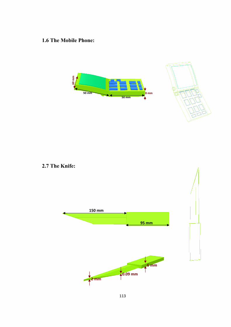
113
1.6 The Mobile Phone:
2.7 The Knife:
50 mm
50 mm
60
mm
8 mm
150 mm
95 mm
6 mm
2 mm 0.09 mm

114
Appendix 2: Author's Publications:
2.1 Journal Papers:
Progress In Electromagnetics Research M, Vol. 26, 55- 68, 2012.
Resolution of Multiple Concealed Threat Objects using Electromagnetic Pulse
Induction
Abdulbast Elgwel1, Stuart William Harmer
2, Nicholas Bowring
3 & Shaofei Yin
4
Sensing & Imaging Group, Manchester Metropolitan University, England
Abstract: The detection and identification of conducting objects using electromagnetic pulses
to excite circulating eddy currents within the object is demonstrated by numerical simulation
using a finite element time domain electromagnetic solver. The ability to discriminate
between objects is based on the decay rate of the induced currents in the object, typically ~
100 µS. The decay rates are different for a wide variety of everyday objects, allowing threat
objects such as handguns, grenades and knives to be discriminated from benign objects such
as mobile phones handsets, watches, keys, etc. Crucially, the time constant characterising an
object depends only upon the electrical properties of the object (conductivity) and the shape
and size of the object; the orientation of the object is irrelevant. This aspect independence of
temporal current decay rate forms the basis of a potential object detection and identification
system. By application of an algorithm based on the generalized pencil of function method,
the authors demonstrate the ability to effectively count and indentify multiple objects carried
in close proximity providing that the objects do not have very similar time constants.
1. Introduction
Pulse Induction techniques for the detection and identification of metallic objects have been
reported and studied as a possible method for concealed weapon detection [1]-[7], both on the
human body and in carried baggage. Electromagnetic Pulse Induction (EMI) relies on a
generating a rapidly changing, spatially uniform magnetic field which penetrates and
encompasses the concealed metallic object. The temporally changing magnetic field induces
transient eddy currents [8]-[13] in the conducting object which then decay by dissipative
(resistive) losses. These eddy currents decay exponentially with time and have a characteristic
time constant which depends only upon the size and shape of the object and the materials
from which it is made; the orientation of the object does not influence the time constant [14]-
[20]. This aspect independence which forms the basis of a simple object identification system:
2 Corresponding author: [email protected]

115
a library of time constants, measured a-priori, can be compared with the measured time
constant of an unknown sample to assess the presence or absence of a particular object or
objects of interest. EMI for concealed object detection has one important advantage over
resonant electromagnetic aspect independent phenomena: that is the human body has a very
much smaller perturbing effect in EMI than at the microwave frequencies (~ 0.4 – 2 GHz )
required for excitation of natural resonances of typical concealed threat objects such as
handguns and knives [21]-[27]. At microwave frequencies the human body is opaque and
scatters and reflects microwave energy very effectively [28], undermining the ability to
extract clean and uncluttered signatures from concealed objects [24], [26]. EMI operates at
much lower frequencies ~ 10 KHz, where the human body is nearly transparent, does not
support appreciable eddy currents and is therefore ‘invisible’ [19]. In the case where
excitation occurs at frequencies where the electromagnetic wavelength is comparable with the
concealed object size (Mie scattering regime), resonant effects give a second aspect
independent parameter: resonant frequency and decay time. However, because EMI operates
at large electromagnetic wavelengths when compared to object size, the concealed object is
electrically small, and there is no resonant condition and consequently there is only one aspect
independent parameter. EMI is at a disadvantage here as mapping an object in complex
frequency space (two independent parameters) provides a less degenerate and more robust
identifier than is possible with a single, aspect independent parameter [29].
2. Theoretical Basis
There is published work in the field of EMI for a variety of uses, concealed weapons
detection [1]-[7]; non destructive testing [30]-[32] ground penetrating radar for unexploded
ordnance detection [18] and mining [17]. These applications rely on the same phenomena and
share a common theoretical underpinning. The time domain dependence of the induced
voltage on the secondary, receiver coil can be expressed as [1],
1n n
n
texpA)t()t(V (1)
where nA and n are the amplitudes and time constants respectively, of the nth eddy current
mode circulating in the object. In general, an analytic solution giving the values of nA and
n is not possible for all, but a few very simple cases where symmetry allows for an
analytical expression. A conducting sphere is one such case [13], [16]. For a sphere of radius
R; conductivity and relative permeability , the time constants n are given by,

116
2
20
n
nR
(2)
where n are the solutions of the equation,
2
n
nn
1
)1()tan(
(3)
The time dependence given by Equation 1 simplifies further for times which are long, when
compared to the time constants of the higher (n ≥ 2) order modes. For example the higher
order modes of a sphere possess shorter time constants than the fundamental, see Equation 2,
and it is assumed that this is true for other, more complex, objects. In this late time regime,
after the excitation pulse or the switching off of the current in the primary coil that provides
the spatially uniform magnetic field, the voltage induced in the secondary coil is simply
1
texpA~)t(V (4)
Thus we may identify an object by its aspect independent, fundamental time constant which is
dependent only upon the shape, size and material that form the object.
When M multiple objects are present within the magnetic field the detected signal, again for
times which are long compared to high order modes, will simply be the superposition of the
signals for the objects individually,
M
1n n
n
texpA~)t(V (5)
3. Object Counting and Identification
A pre-requisite of a security screening system based on EMI is the capability to detect and
classify multiple objects that may be within close proximity to one another. As an example, a
person could quite conceivably be carrying a handgun in a briefcase, a knife in their pocket
and may well also have a mobile phone and other benign objects on their person. A robust
and effective EMI based system is required to detect, count and identify these objects
whatever their separations. Without doubt, the most serious problem posed by application of
aspect independent EMI techniques is that of a single parameter being used to identify a
concealed object, the fundamental time constant. There is an inherent degeneracy in this
approach which may well prevent certain objects that share similar time constants being
counted as individual items and therefore discriminated from one another. As can be seen
from Equation 2, an object's time constant may be matched by an appropriately sized sphere.

117
To ascertain whether this problem is significant enough to seriously limit the effectiveness of
an EMI system requires the measurement or simulation of a very wide variety of objects, both
threat and non-threat, which may be encountered. In this study the authors present a
representitive study of six commonly carried objects: A wristwatch, key and mobile phone
handset as representative of benign objects and a knife, handgun and hand grenade as
representative of threat objects.
Non-linear recursive fitting algorithms are not particularly suitable for the extraction of
multiple time constants from a decaying temporal signal of the form of Equation 5. The fitting
is sensitive to the starting points and is slow and computer intensive. The greatest problem is
counting the number of objects present, as this is generally unknown a-priori and applying a
model with an increasing number of fit parameters, terms and starting points quickly results in
an unwieldy and unreliable method. The authors have investigated the application of the
Generalised Pencil of Function (GPOF) method [33]-[34], which is a far more suitable and
rapid algorithm for the intended application as it is a generalised Eigen value problem and
therefore does not need multiple iterations to arrive at a solution. This approach is suggested
by Geng et al. [19] for the extraction of time constants from non resonant objects.The GPOF
algorithm decomposes the signal into a discrete set of complex frequency components; in the
case of an exponentially decaying signal of the form of Equation 5, only the real parts of the
complex frequency are non-zero and the imaginary (oscillatory) frequencies are ignored. The
number of objects M is unknown but can be estimated, in the absence of degeneracy of time
constants, by iteratively increasing the model order (the number of complex frequencies
expected) of the GPOF algorithm until any new complex frequencies found have amplitude
which is lower than a preset threshold value. See Figure 1. Comparison of the time constants
thus obtained can then be made with a library of time constants for common or expected
objects and a list of likely carried objects may then be formed. Output may be an autonomous
alarm or informing the user, by screen, that a person is carrying only benign objects or that a
person is likely carrying a threat object or objects.
The simulated transient data were windowed by selecting the temporal data 100 μS after the
current driving the magnetic field is turned off. This is done to weight the fundamental
resonance of the object. If this is not done spurious detections can arise, as higher order time
constants can have sufficient amplitude to confuse the system, meaning a single object could
be counted as two or more objects and the higher order time constants possibly mistakenly
identified as being the fundamental time constants of other objects which are not actually
present. 100 μS was chosen as this is the longest time constant of the limited objects
simulated, with the exception of the hand grenade which has an unusually long time constant.

118
However this choice of waiting 100 μS is a somewhat arbitrary choice as the exact start of the
late time is dependent on the object; for spheres the start of the late time region is given as the
period of the fundamental time constant [13] and for handgun sized objects as ~ 100 μS [6]. A
threshold discriminator of 5% of the maximum amplitude is applied to the amplitudes
extracted using GPOF, below this value the associated time constant is not recorded.
Figure 1: Flowchart depicting the processing steps and application
of the GPOF algorithm to extract multiple time constants
from the receiver coil time data.
4. Simulation
Numerical simulation is carried out using the commercially available finite element, time domain,
electromagnetic solver software from Vector Fields. A large, circular coil is suitable for the purpose of
generating a spatially uniform field over distances that are commensurate to typical concealed weapon
Yes
No
Time window data
to extract
fundamental time
constants
Application of GPOF
algorithm
Has amplitude
of decay terms
fallen below
threshold
value?
Add 1 to
model
order
Library
of time
constant
s
Number of objects detected
set to model order. Compare
time constants with library
Display
objects
detected
Coils

119
sizes (~20 cm). The model was validated by simulation of stainless steel spheres (conductivity 1.1×10⁶
sm-1
) and different radii. The fundamental time constants from simulations were compared to Equation
2, and the simulated results agree well with theory see table I.
Table I: Comparison of theoretical and simulated recovered time constants
for stainless steel spheres of different radii
The influence of the separation of two spheres (radii 4 and 6 cm) where simulated at varying
separations, see Table II and both time fundamental time constants where accurately recovered
irrespective of the separation between the two spheres. This important as it suggests that multiple
objects can be detected and identified by means of their time constants even when they are located
close together, for example when carried in a bag, providing they are not in direct electrical contact.
Table II: Influence of object separation on two stainless steel spheres (radii 4 and 6
cm respectively). The separation indicated between objects is for their closest
surfaces and there is no electrical contact for the zero separation case.
5. Results
The aspect independence of the time constant of objects is the central and key effect on which
the potential of EMI for concealed threat screening rests. A handgun was simulated in four
different orientations (see figure 3) and the fundamental time constant recovered in the
Material Radius
cm
Time Constant µS
(simulation)
Time Constant µS
(theory)
Stainless
Steel
3.0 121 126
4.0 221 224
5.0 350 350
6.0 507 504
Material Objects
separation - cm
Time Constant one
- µS
Time Constant two -
µS
Stainless
Steel
100 221 526
50 215 529
25 220 527
0.2 223 526
0.0 222 527

120
absence of noise, there is little variation between the aspects, see Table III. Similar aspect
independence is reproduced for the other simulated objects listed in Table IV.
Figure 3: Examples of simulations of a handgun and hand grenade in the space between
the drive (larger coil) and receiver (smaller coil) and some orientations of handgun used
to validate the aspect independent nature of an object's time constant - see Table III.
Side on
Flat
Barrel down
Barrel Up

121
Table III: Influence of object orientation
Six objects were simulated in a single aspect, three benign objects and three threat objects.
These were simulated individually and their characteristic time constants obtained in the
absence of noise by the process described in Figure 1.
Figure 4: Five of the six items and their fundamental time constants as measured
Material Object & orientation
Time Constant
µS
Stainless steel Handgun
Side on 72.4
Barrel up 72.1
Barrel down 72.0
Flat 73.6
Mobile Phone
24.1 µS
Wrist Watch 56.1
µS
Hand Grenade 250
µS
Knife 63.8
µS
Key 17.2
µS

122
when the object is simulated individually without noise; the handgun is shown in Figure 3 and
has a fundamental time constant of 72.4 μS. See table IV for grouped objects results. All
objects are stainless steel.
Table IV: Groups of two to five objects and the fundamental time constants
obtained from these groupings; comparison is made to the time constants
obtained for the Individual objects.
The time constants for these objects are presented in Table IV along with the retrieved time
constants for groups composed of different numbers of the six simulated objects. The time
constants are retrieved under noise free conditions (SNR of _) and with different levels of
Gaussian noise applied (SNR of 100, 50 and 10). The hand grenade has by far the longest
time constant, which is related to its near spherical and smooth shape giving rise to relatively
5 Results with a greater than 10% discrepancy to the individually measured time constants
Objects
SNR
Hand
grenade
250 µS
Handgun
72.4 µS
Knife
63.8 µS
Wrist
watch
51.6 µS
Mobile
phone
24.1 µS
Key
17.2 µS
Hand grenade &
handgun
Infinity 250 74.7 - - - -
100 245.01 34.05 - - - -
50 240.16 14.52 - - - -
10 224.26 - - - - -
Wrist watch &
key
Infinity - - - 53.9 - 12.45
100 - - - 44.22 - -
50 - - - 46.60 - -
10 - - - 51.30 - -
Hand grenade,
handgun & wrist
watch
Infinity 253 86.01
- 52.0 - -
100 237.69 64.4 - - - -
50 215.17 59.06 - - - -
10 201.77 - - - - -
Hand grenade,
handgun, wrist
watch & knife
Infinity 252 77.4 79.51
43.01
- -
100 235.85 27.63 - -
- -
50 210.27 39 - -
- -
10 204.001 - - -
- -
Hand grenade,
handgun, wrist
watch, knife &
mobile phone
Infinity 250 75.1 65.5 53.6 20.91
-
100 231.96 74.84 - - -
-
50 226.47 43.6 - -
-
10 230.88 32.46 - - -
-
Hand grenade,
handgun, knife,
mobile phone &
key
Infinity 232
69.1 65.6 - 25.1 9.251
100 222.20 54.19 33.46 - - -
50 221.46 30.55 - - - -
10 212.24 26.58 - - - -

123
long lived eddy current distributions. Application of the simple algorithm described to the
simulations of multiple objects, in the absence of noise, comprising combinations of the six
objects listed in Table IV, successfully retrieves the fundamental time constants of the
individual objects reasonably accurately. There is some discrepancy of time constants,
notably in groups that contain more objects. The key seems to pose the greatest problem, the
fundamental time constant is not accurately estimated when it is included in a group of other
objects (See Table IV). The inaccuracy is probably due to the small size of the key relative to
the other objects; the small size giving a much shorter fundamental time constant and a
weaker contribution to the signal compared to the other, larger, objects. This results in the
signals from the larger objects dominating and a greater inaccuracy in the retrieved time
constant. However this interpretation seems to be incompatible with the data obtained for two
spheres in proximity; see Table II, where the larger sphere's time constant is less accurately
determined than the smaller.
When noise is added to the signal at a relatively low level (SNR of 100), the identification of
multiple objects is significantly impaired, with only the largest and dominant objects being
counted and the smaller objects either missing or their time constants considerably corrupted
to the extent that identification would not be possible. For example, in the case where the
handgun, hand grenade and wristwatch are presented together, only the handgun and hand
grenade are counted for an SNR of 100; the wristwatch is absent. As the SNR increases the
situation worsens, for an SNR of 10, using the same example scenario, only one object is
counted (the hand grenade) and the time constant is highly corrupted (~20% different from
accepted value). With five items present the addition of noise prevents the smaller objects
from being counted and corrupts the time constants so that identification is not feasible, in
fact only the hand grenade, which has a large cross section and long time constant, seems to
remain detectable and identifiable.
7. Summary
The simulations demonstrate the feasibility of being able to detect, count and identify a range
of commonly carried objects and also a range of weapons. However, this capability is lost if
the signal is noisy and under these conditions smaller objects are not detected and aspect
independent time constants are significantly corrupted, rendering identification unlikely. SNR
must be better than 100 if the proposed technique is to have reasonable chance of success. If
SNR can be kept suitably low then discrimination of weapons from benign objects is feasible,
at least for the objects simulated, as the fundamental time constants are sufficiently distinct.

124
The presence of multiple objects within the sensor range does not prevent counting and
identification, although the accuracy of the determination of the individual objects'
fundamental time constants is made worse increasing number of objects. The reason for this
worsening of performance is undoubtedly due to the interaction (scattering) of the magnetic
fields from the objects, i.e. the eddy currents flowing in one object give rise to a changing
magnetic field which induces eddy currents in neighbouring objects and therefore blurs the
time constants. In the absence of noise, the distortion of time constants when multiple objects
are present is not so strong as to prevent the counting and identification of five objects from
one another, with the possible exception of the key, see Table IV. Smaller objects such as a
key or coins are more difficult to indentify due to their smaller cross section when compared
to objects such as a handgun, hand grenade or knife. This is not expected to constitute a
serious problem as most threat objects are significantly larger than a key or a coin. This
investigation is now being extended to the laboratory, where a demonstrator system is now
being built and it is anticipated that this work will enhance the capability of current screening
procedures.
References
1. Nelson, C. V., Cooperman, C. B., Schneider, W., Wenstrand, D. S., and Smith,
D. G., “Wide Bandwidth Time-Domain Electromagnetic Sensor for Metal
Target classification,” IEEE Trans. Geosci. RemoteSens. 39(6), 1129–1138
(Jun 2001).
2. Nelson, C. V., “Wide-Area Metal Detection System for Crowd Screening,” in
Proc. SPIE AeroSense 2003 Conf., Sensors and Command,
Control,Communication, and Intelligence (C3T) Technologies for Homeland
Defense and Law Enforcemnt II, Orlando, FL (22–25 Apr 2003).
3. C. V. Nelson, "Metal Detection and Classification Technologies", Johns
Hopkins APL technical Digest, Vol. 24, Number 1, 2004, pp. 62-66.
4. Nicholas G. Paulter, “Guide to the Technologies of Concealed Weapon and
Contraband Imaging and Detection,” NIJ Guide 602–00 Electricity Division,
National Institute of Standards and Technology Gaithersburg, MD 20899.
Prepared for: National Institute of Justice Office of Science and Technology
Washington, DC 20531 February 2001.
5. Alan Agurto, Yong Li, Gui Yun Tian, Nick Bowring and Stephen Lockwood,
“A Review of Concealed Weapon Detection and Research in Perspective,”

125
Proceedings of the 2007 IEEE International Conference on Networking,
Sensing and Control, London, UK, 15-17 April 2007
6. Agurto Goya, Alan, “New Proposal for the Detection of Concealed Weapons:
Electromagnetic Weapon Detection for Open Areas,” Thesis PhD. 2009,
Huddersfield UK.
7. Hunt, A.R., Hogg, R.D., and Foreman, W., “Concealed weapons detection
using electromagnetic resonances,” Proc. of the SPIE, The International
Society for Optical Engineering Conference of Enformcement and Security
Technologies, Vol. 3575, pp. 62-67, Boston, MA. November 1998.
8. Baum, C. E., “On the singularity expansion method for the solution of
electromagnetic interaction problems,” Interaction Notes, Note 88, Air Force
Weapons Laboratory, 1971.
9. Baum, C. E., E. J. Rothwell, K. M. Chen, et al., “The singularity expansion
method and its application to target identification,” Proc. IEEE, Vol. 79, No.
10, 1481-1492, 1991.
10. Wang, Y. and N. Shuley, “Complex resonant frequencies for the identifcation
of simple objects in free space and lossy environments,” Progress In
Electromagnetics Research, Vol. 27, 1-18, 2000.
11. S. W. Harmer, S. E. Cole, N. J. Bowring, N. D. Rezgui, and D. Andrews, “On
body concealed weapon detection using a phased antenna array,” Progress In
Electromagnetics Research, Vol. 124, 187-210, 2012
12. Harmer, S. W., D. A. Andrews, N. D. Rezgui, and N. J. Bowring, “Detection
of handguns by their complex natural resonant frequencies," IET Microw.
Antennas Propag., Vol. 4, No. 9, 1182-1190, Sep. 2010.
13. Harmer, S., D. Andrews, N. Bowring, N. Rezgui, and M. Southgate, “Ultra
wide band detection of on body concealed weapons using the out of plane
polarized late time response,” Proc. SPIE, Vol. 7485, 748505, 2009.
14. Zhang, L., Hao, Y., and Parini, C.G. “Natural resonant frequency extraction
for concealed weapon detection at millimetre wave frequencies,” 2nd
European Conference on Antennas and Propagation (EuCAP 2007)
(2007/11961), Edinburgh, UK, 11-16 Nov. 2007.
15. Clive M. Alabaster, “The microwave properties of tissue and other lossy
dielectrics,” PhD. thesis, Cranfield UK, March 2004.

126
16. A. A. Kaufman, P. A. Eaton, “The Theory of Inductive Prospecting,”
Amsterdam, Netherland, 2001.
17. Norbert Geng and Carl E. Baum, “On the Low-Frequency Natural Response
of Conducting and Permeable Targets,” IEEE Transactions on geoscience and
remote sensing, Vol. 37, No. 1, Jan. 1999
18. C. E. Baum, “Low-frequency near-field magnetic scattering from highly, but
not perfectly, conducting bodies,” Phillips Lab., Interaction Note 499, Nov.
1993.
19. G. D. Sower and S. P. Cave, “Detection and identification of mines from
natural magnetic and electromagnetic resonances,” in Proc. SPIE, Orlando,
FL, vol. 2496, pp. 1015–1024, 1995.
20. G. D. Sower, “Eddy current resonances of canonical metallic targets—Theory
and measurements,” EG&G MSI, Interaction Note, Feb. 1997.
21. Gui Yun Tian, Ali Sophian, David Taylor, and John Rudlin, “Multiple Sensors
on Pulsed Eddy-Current Detection for 3-D Subsurface Crack Assessment,”
IEEE Sensors Journal, 5 (1). pp. 90-96, 2005.
22. Wait, J.R., and Kenneth P. Spies, “Quasi-static Transient Response of a
Conducting Permeable Sphere,” Geophysics,” Vol. 34, issue 5, p. 789-792,
1969.
23. Hua, Y. and T. K. Sarkar, "Generalized pencil-of-function method for
extracting poles of an EM system from its transient response," IEEE Trans.
Antennas Propag., Vol. 37, No. 2, 229-234, 1989.
.

127
2.2 Conference Papers:
Research day at Manchester Metropolitan University, 20th
April 2012
Detection of Metallic Objects using Electromagnetic Pulses
Abdulbast Elgwel, Nicholas Bowring and Stuart Harmer, Sensing and imaging
group, School of Science and Engineering, Manchester Metropolitan University,
Oxford Road, Manchester M1 5GD
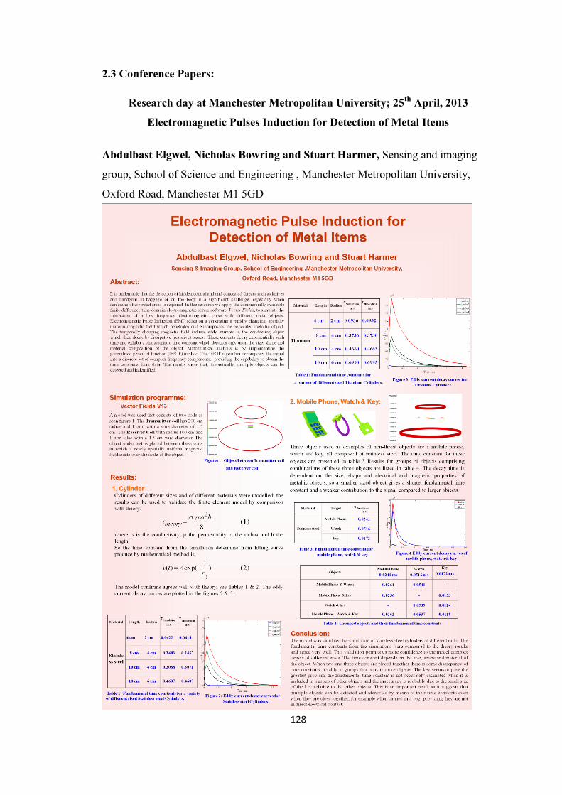
128
2.3 Conference Papers:
Research day at Manchester Metropolitan University; 25th
April, 2013
Electromagnetic Pulses Induction for Detection of Metal Items
Abdulbast Elgwel, Nicholas Bowring and Stuart Harmer, Sensing and imaging
group, School of Science and Engineering , Manchester Metropolitan University,
Oxford Road, Manchester M1 5GD