abhinay kuchikulla thesis - ittc home
TRANSCRIPT
Design and Development of a Wideband
Coherent Radar Depth Sounder
By
Abhinay Kuchikulla
B.E., Electronics and Communication Engineering,
Osmania University, 2001
Submitted to the Department of Electrical Engineering and Computer Science and the
Faculty of the Graduate School of the University of Kansas in partial fulfillment of
the requirements for the degree of Master of Science.
Thesis Committee
Chairperson: Sivaprasad Gogineni
Christopher Allen
Pannirselvam Kanagaratnam
Date of Defense: May 21st, 2004

ACKNOWLEDGEMENTS
I would like to thank Dr. Prasad Gogineni for giving me an opportunity to
work on this thesis, which is an imperative part of the PRISM project. I would like to
thank him for his guidance throughout this thesis and for his suggestions and support
during my graduate studies here at KU. I would like to thank Dr. Christopher Allen
and Dr. Pannirselvam Kanagaratnam for their valuable suggestions during my
research work and for serving on my thesis committee. I would like to express my
apprepreation for the support provided by NSF and NASA through Grant #OPP-
0122520 (NSF) and Grant #NAG5-12659 and NAG5-12980 (NASA).
I would like to extend my sincere and utmost gratitude to Mr. Torry Akins and
Mr. Saikiran Namburi for their invaluable guidance, advice, encouragement and
inspiration throughout my thesis. I am greatly indebted to Mr. Torry Akins for
guiding me towards being a better engineer. I take this opportunity to thank Ms. Kelly
Mason for patiently editing my thesis report and helping me with managerial support.
Special thanks to Mr. Dennis Sundermeyer for his time and effort in assembling the
radar.
I would like to dedicate this thesis to my parents, Ramesh and Swarna for
their endless love and support. This work would not have been possible without the
strong support I received from my brother, Ajay. I would like to thank all the students
in Remote Sensing Laboratory (RSL) for their help throughout my thesis. Finally, but
not the least, I thank all my friends in Lawrence for the wonderful time I spent with
them, which I will cherish for the rest of my life, GO Jayhawks.
ii
ABSTRACT
Sea level rise is an important indicator of global climate change. Sea level has
been increasing at about 2mm/year over the past century and may continue to do so.
The continuing rise in sea level will have a devastating impact on humanity as
approximately 60% of people on this planet live in the coastal regions. The polar ice
sheets, which account for 80% of earth’s fresh water supply are a major source of sea
level rise. A key to quantifying their contribution is an accurate determination of the
mass balance of these ice sheets. Ice thickness is an important parameter required to
estimate the mass balance of the ice sheet and to study ice dynamics. Depth sounding
radars designed at RSL/KU have been successful in measuring the ice thickness for
the past 10 years.
A Wideband Coherent Radar Depth Sounder System has been developed to
obtain better delineation of the internal layers and information about the bedrock
properties. The radar operates over a frequency range of 50-200 MHz, providing a
resolution of less than 1 m in ice. A high speed Arbitrary Waveform Generator
(AWG) is used to generate a chirp from 50-200 MHz over a very small pulse width to
obtain large unambiguous range and the maximum number of integrations. Two gain
channels are incorporated into the receiver to obtain very high dynamic range. The
low gain channel is used to map the shallow internal layers and the HGC provides ice
sheet thickness and bedrock properties up to a depth of 4500 m. The gain in both the
channels can be altered depending on the operating mode, ice thickness, and
iii
operating environment to obtain optimum performance. A high-speed data acquisition
system is used to digitize and perform necessary real time processing on the data
before transferring it to the storage device. The radar and data-acquisition systems
have been significantly miniaturized using the latest RF and fabrication technology.
The entire system has been designed to fit into multiple compact-PCI cards.
Laboratory tests show that the radar system has the required sensitivity to map 4500-
m-thick ice. Considerable improvement in sidelobe performance was achieved. The
radar system will be tested during the Summer 2004 field experiment at Summit
Camp, Greenland.
iv

Table of Contents
Chapter 1.................................................................................................... 1
Introduction............................................................................................ 1
1.1 Motivation and Objectives of Studying Glacial Ice.............................. 1
1.2 Objectives of the PRISM project .......................................................... 3
1.3 Objectives, Approach and Overview of the report ............................... 5
Chapter 2.................................................................................................... 7
Introduction to Ice Sounding Radars ..................................................... 7
2.1 History of Radio-Echo Sounding.......................................................... 7
2.2 Work done at KU ................................................................................ 10
Chapter 3.................................................................................................. 17
Ice Sheet Model and System Parameters ............................................. 17
3.1 Introduction......................................................................................... 17
3.2 Ice sheet model.................................................................................... 17
3.3 Attenuation through Ice ...................................................................... 18
3.4 Derivation of system specifications .................................................... 25
v

Chapter 4.................................................................................................. 34
Wideband Coherent Radar Depth Sounder ......................................... 34
4.1 System overview and operation .......................................................... 34
4.2 Control Signals and their Timing........................................................ 38
4.3 Transmitter .......................................................................................... 39
4.4 Receiver .............................................................................................. 42
4.5 Frequency Synthesizer (10 MHz to 500 MHz)................................... 55
Chapter 5.................................................................................................. 59
System Housing and Results................................................................. 59
5.1 WCORDS Prototype ........................................................................... 59
5.2 System Housing .................................................................................. 60
5.3 Results ................................................................................................. 63
Chapter 6.................................................................................................. 74
Conclusions and Future Recommendations......................................... 74
6.1 Conclusions......................................................................................... 74
6.2 Future Recommendations ................................................................... 75
vi
List of Figures
Figure 3.1 Ice Sheet Model......................................................................................... 18
Figure 3.2 Attenuation through ice at different acidic levels...................................... 24
Figure 3.3 Front end part of the Receiver affecting the noise figure of the system.... 27
Figure 3.4 Low gain receiver chain ............................................................................ 32
Figure 4.1 WCORDS Block diagram ......................................................................... 35
Figure 4.2 WCORDS Timing ..................................................................................... 38
Figure 4.3 WCORDS Transmitter .............................................................................. 39
Figure 4.4 Transmitter Schematic Diagram................................................................ 41
Figure 4.5 Transmitter Board...................................................................................... 41
Figure 4.6 WCORDS Receiver Front End.................................................................. 43
Figure 4.7 Front Bandpass Filter ................................................................................ 44
Figure 4.8 Receiver Blanking Switch ........................................................................ 45
Figure 4.9 Low Noise Amplifier................................................................................. 46
Figure 4.10 Bandpass Filter ........................................................................................ 47
Figure 4.11 Coupler (20 dB)....................................................................................... 47
Figure 4.12 Receiver Front End Schematic ................................................................ 48
Figure 4.13 Receiver Front End Board ....................................................................... 48
Figure 4.14 High Gain Channel Block Diagram ........................................................ 49
Figure 4.15 High Gain Blanking Switch..................................................................... 49
Figure 4.16 Digital Attenuator.................................................................................... 50
Figure 4.17 High Gain Amplifier................................................................................ 51
vii
Figure 4.18 Final Amplifier ........................................................................................ 52
Figure 4.19 High Gain Channel Schematic ................................................................ 52
Figure 4.20 High Gain Channel Board ....................................................................... 53
Figure 4.21 WOCRDS Low Gain Channel................................................................. 53
Figure 4.22 Low Gain Channel Schematic ................................................................. 54
Figure 4.23 Low Gain Channel Board........................................................................ 54
Figure 4.24 10 MHz to 500 MHz Frequency Synthesizer .......................................... 56
Figure 4.25 10-MHz to 500-MHz Frequency Synthesizer Schematic........................ 57
Figure 4.26 10-MHz to 500-MHz Frequency Synthesizer Board............................... 58
Figure 5.1 WCORDS Prototype and the final version................................................ 60
Figure 5.2 WCORDS modules mounted inside Aluminum compact PCI cards ........ 62
Figure 5.3 Transmitter and Receiver compact PCI cards mounted inside Euro Cage 62
Figure 5.4 Transmitter Amplitude Response with Tx Blk ON................................... 64
Figure 5.5 Transmitter Amplitude Response with Tx Blk OFF ................................. 64
Figure 5.6 Receiver Amplitude response with Rx and HG Blk OFF ......................... 65
Figure 5.7 Receiver Amplitude response with Rx Blk ON and HG Blk OFF............ 66
Figure 5.8 Receiver Amplitude response with Rx and HG Blk OFF ......................... 66
Figure 5.9 Receiver Transients ................................................................................... 67
Figure 5.10 Transmit Chirp at the output of the AWG............................................... 69
Figure 5.11 Received Chirp at the output of the HGC ............................................... 69
Figure 5.12 Received chirp and its Impulse response................................................. 71
Figure 5.13 Impulse response of ideal and recorded signals ...................................... 71
viii

Figure 5.14 Amplitude and Phase corrected transmit and received signal ................. 72
Figure 5.15 Impulse response of ideal, un-corrected and corrected signals ............... 72
ix

List of Tables
Table 2-1 Various time-domain radars used in radioglaciology................................... 9
Table 2-2 System Parameters of CARDS, NGCORDS and ACORDS...................... 13
Table 3-1 Compression Points of Front end components........................................... 33
Table 4-1 WCORDS System Parameters ................................................................... 37
Table 5-1 Amplitude of Transients generated due to switching ................................. 67
Table 5-2 Sidelobe performance................................................................................. 73
Table 5-3 Frequency Synthesizer performance .......................................................... 73
x
Chapter 1
Introduction
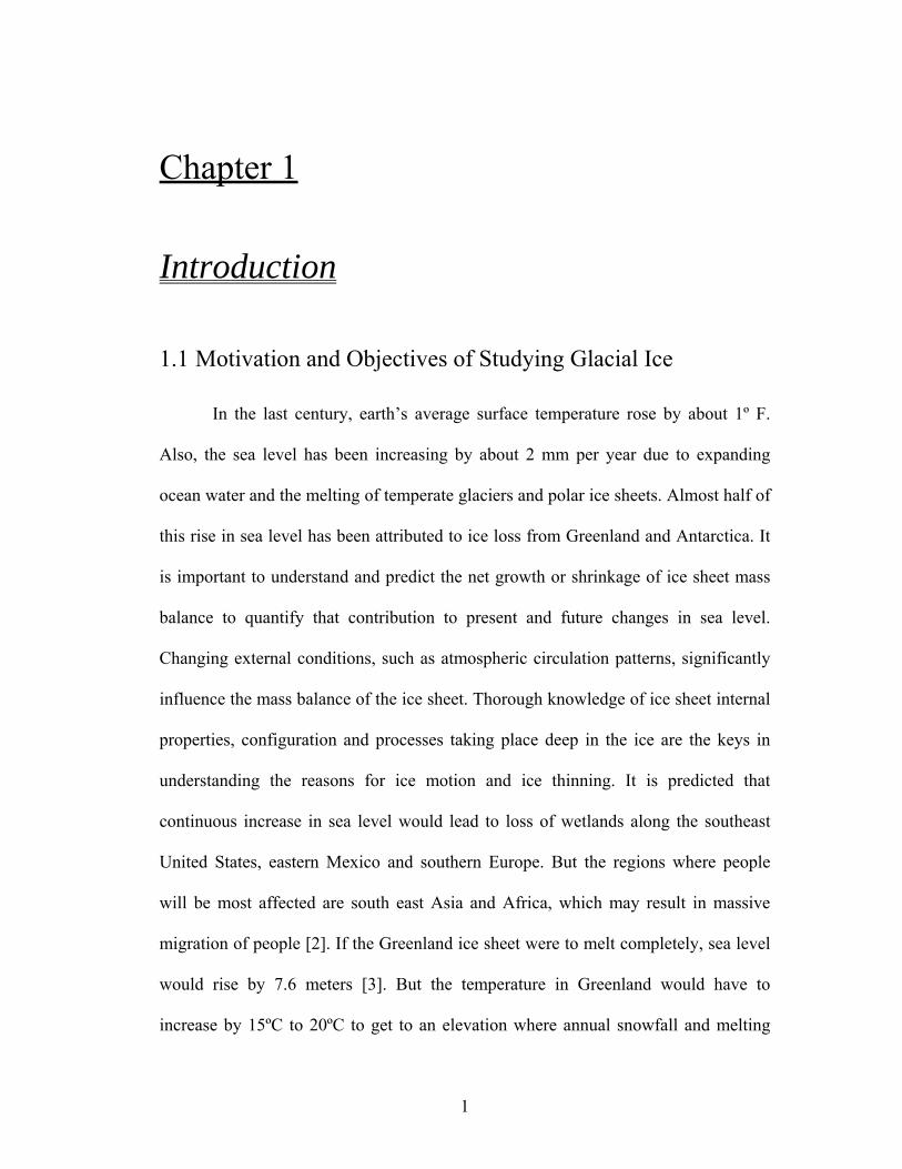
1.1 Motivation and Objectives of Studying Glacial Ice
In the last century, earth’s average surface temperature rose by about 1º F.
Also, the sea level has been increasing by about 2 mm per year due to expanding
ocean water and the melting of temperate glaciers and polar ice sheets. Almost half of
this rise in sea level has been attributed to ice loss from Greenland and Antarctica. It
is important to understand and predict the net growth or shrinkage of ice sheet mass
balance to quantify that contribution to present and future changes in sea level.
Changing external conditions, such as atmospheric circulation patterns, significantly
influence the mass balance of the ice sheet. Thorough knowledge of ice sheet internal
properties, configuration and processes taking place deep in the ice are the keys in
understanding the reasons for ice motion and ice thinning. It is predicted that
continuous increase in sea level would lead to loss of wetlands along the southeast
United States, eastern Mexico and southern Europe. But the regions where people
will be most affected are south east Asia and Africa, which may result in massive
migration of people [2]. If the Greenland ice sheet were to melt completely, sea level
would rise by 7.6 meters [3]. But the temperature in Greenland would have to
increase by 15ºC to 20ºC to get to an elevation where annual snowfall and melting
1
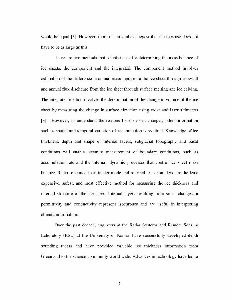
would be equal [3]. However, more recent studies suggest that the increase does not
have to be as large as this.
There are two methods that scientists use for determining the mass balance of
ice sheets, the component and the integrated. The component method involves
estimation of the difference in annual mass input onto the ice sheet through snowfall
and annual flux discharge from the ice sheet through surface melting and ice calving.
The integrated method involves the determination of the change in volume of the ice
sheet by measuring the change in surface elevation using radar and laser altimeters
[3]. However, to understand the reasons for observed changes, other information
such as spatial and temporal variation of accumulation is required. Knowledge of ice
thickness, depth and shape of internal layers, subglacial topography and basal
conditions will enable accurate measurement of boundary conditions, such as
accumulation rate and the internal, dynamic processes that control ice sheet mass
balance. Radar, operated in altimeter mode and referred to as sounders, are the least
expensive, safest, and most effective method for measuring the ice thickness and
internal structure of the ice sheet. Internal layers resulting from small changes in
permittivity and conductivity represent isochrones and are useful in interpreting
climate information.
Over the past decade, engineers at the Radar Systems and Remote Sensing
Laboratory (RSL) at the University of Kansas have successfully developed depth
sounding radars and have provided valuable ice thickness information from
Greenland to the science community world wide. Advances in technology have led to
2
improvements in depth sounding radars, making them smaller, more efficient and
more reliable. New and effective algorithms have been developed to process recorded
data to obtain accurate information about the ice sheet, such as ice thickness, surface
roughness, surface elevation, surface topology, ice accumulation, etc.
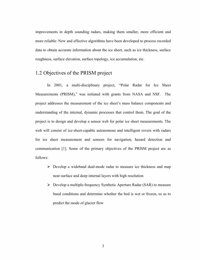
1.2 Objectives of the PRISM project
In 2001, a multi-disciplinary project, “Polar Radar for Ice Sheet
Measurements (PRISM),” was initiated with grants from NASA and NSF. The
project addresses the measurement of the ice sheet’s mass balance components and
understanding of the internal, dynamic processes that control them. The goal of the
project is to design and develop a sensor web for polar ice sheet measurements. The
web will consist of ice-sheet-capable autonomous and intelligent rovers with radars
for ice sheet measurement and sensors for navigation, hazard detection and
communication [1]. Some of the primary objectives of the PRISM project are as
follows:
Develop a wideband dual-mode radar to measure ice thickness and map
near-surface and deep internal layers with high resolution
Develop a multiple-frequency Synthetic Aperture Radar (SAR) to measure
basal conditions and determine whether the bed is wet or frozen, so as to
predict the mode of glacier flow
3

Develop automated rovers to support multiple radars and the sensor web
with minimum human intervention, thus allowing the radars to be operated
in harsh environments
Develop networking and control capabilities for supporting the sensor web
and provide automated collection and processing of data and transmittal of
it to a central archive
Develop various geophysical and electromechanical models of ice sheets
based on recorded data
Collect data over test sites in Greenland and Antarctica successfully
The PRISM project involves multidisciplinary groups working to achieve the
goals mentioned above:
Radar design and simulations
Data analysis and visualization
Wideband antenna design
Robotics
Information Systems
During the summer of 2003, prototypes and basic working concepts of all the
radars, robotic rovers and networking wireless links were tested in northern
Greenland at the North Greenland Ice Core Project camp (NGRIP), operated by the
Danish government.
4
1.3 Objectives, Approach and Overview of the report
The primary objective of this project is to develop a Wide-Band Coherent
Radar Depth Sounder (WCORDS) to meet the following PRISM project
requirements:
Measure the ice thickness up to a depth of 4km
Obtain important information about ice sheet basal properties and
scattering characteristics at different frequencies
Map the deep internal layers with a range resolution of less than 1-2m in
ice to estimate the history of past climate information and glacier
deformation and also provide crucial validation of theoretical models
Provide the flexibility of altering radar parameters to obtain optimum
performance under different operating modes and environments
Provide the ability to remove phase and amplitude nonlinearities of the
system from the recorded data
Miniaturize the radar system to fit into compact PCI cards
Optimize the radar to be operated on both surface-based and airborne
platforms
The approach was to first develop a fully operational prototype radar to
validate the working of the concept and to check for any unseen errors and possible
needs for improvement in and among the modules. This prototype was field tested
during the 2003 field season. After the summer field experiment, an improved and
miniaturized version of the Wideband Coherent Radar Depth Sounder was developed.
5

Chapter 2 covers a brief description of the history of Radio-Echo Sounding,
followed by discussion of the work done at RSL and the recent depth sounders
developed at RSL (NGCORDS and ACORDS), their limitations and problems, and
advantages of WCORDS over them. Chapter 3 discusses the ice sheet model and
losses associated with it. Derivation of important system parameters is also covered in
the third chapter. Chapter 4 deals with the design and development of WCORDS and
the 500-MHz frequency synthesizer required to support the digital system. Simulation
and laboratory test results are included in Chapter 5. The concluding chapter covers
future recommendations and suggestions to refine WCORDS.
6

Chapter 2
Introduction to Ice Sounding Radars
2.1 History of Radio-Echo Sounding
The roots of Radio-Echo Sounding (RES) can be traced way back to 1933,
when it was discovered at Admiral Byrd’s base, Little America, Antarctica, that snow
and ice appeared transparent to high-frequency radio signals. Later reports on the
failure of radar altimeters over ice when operated in VHF and UHF bands led Waite
and others to demonstrate in 1957 that a radar altimeter could be used to measure the
thickness and other characteristics of polar glaciers [7, 8 and 9]. This development
added a new chapter in the study of glaciology. Within 6 years after Waite’s
demonstration, the first of several VHF Radio-Echo Sounders was developed by
Evans at Cambridge University’s Scott Polar Research Institute (SPRI). The
application of radio-echo sounding to glaciology generated interest among various
research groups worldwide. During the 1960s and early 1970s, several research
groups worldwide began developing and using first-generation RES systems. These
RES systems operating between 30 MHz and 600 MHz, were successful in sounding
ice sheets, glaciers and ice caps in Greenland and Antarctica. RES thickness estimates
7
when compared against results obtained from seismic and gravitational methods,
agreed to within 2 percent [3 and 10].
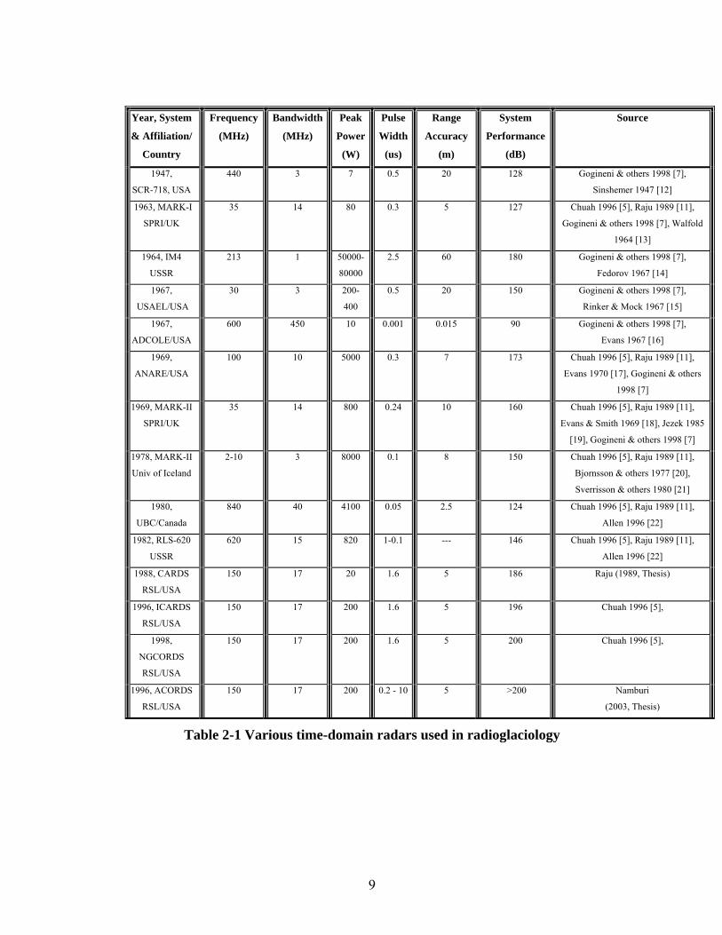
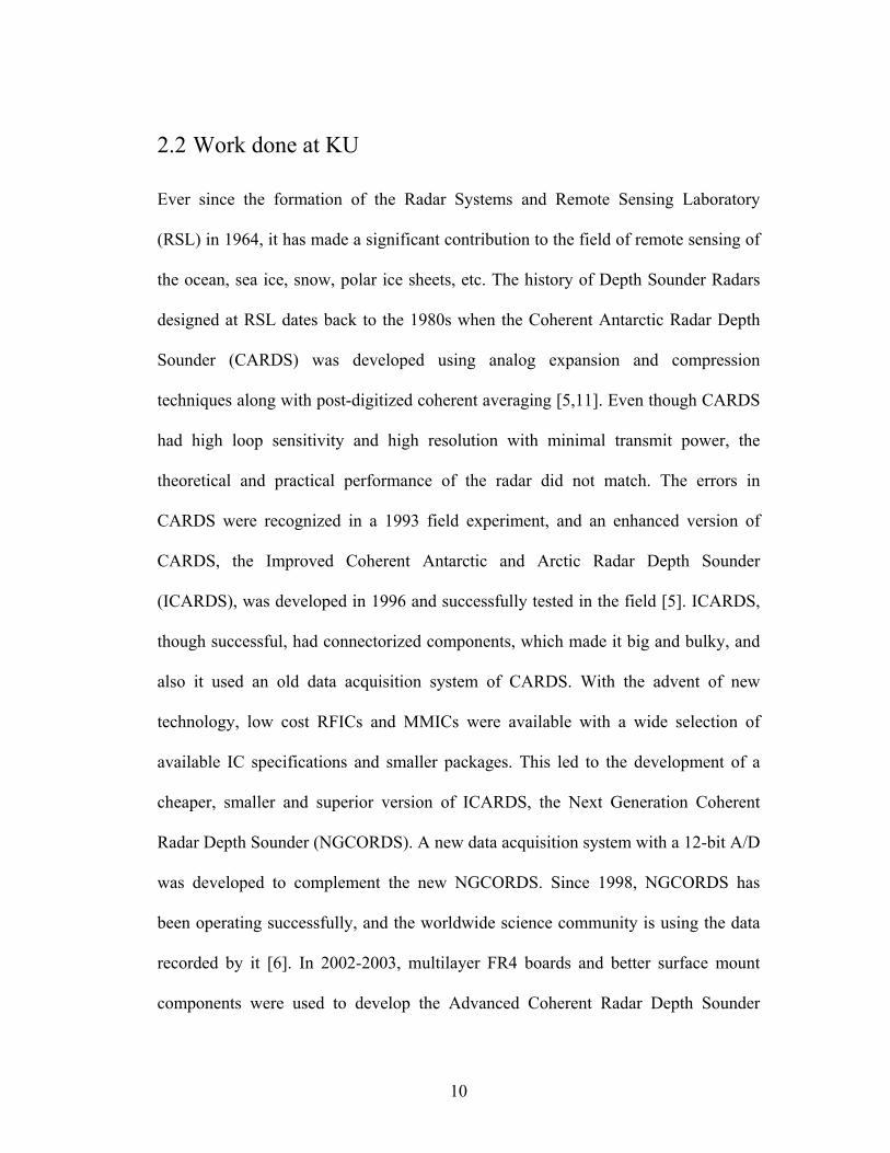
By the mid 1970s, RES became one the most efficient and easiest methods for
determining bedrock topography, ice thickness and internal layering. Initially, the
RES systems were designed to estimate the ice thickness and layering information of
the ice sheets, but soon it was realized that other important characteristics and
features of polar ice could be estimated from the collected data. The second-
generation of RES systems were designed to cater to a specific type of ice models,
such as valley glaciers, cold thick ice sheets and warm ice sheets with liquid water
present at the bottom. By the 1990s, with the advent of new technology and
advancements in computing, digital systems, semiconductor devices and GPS
systems, RES systems were becoming more compact, efficient and capable of relating
data to a location with a resolution of 2-5 m. The third-generation RES systems were
emerging to address specific glaciological questions. Table (2.1) provides a brief
summary of various time-domain radar sets reported in the literature [5, 6, 7 and 11].
8
Year, System
& Affiliation/
Country
Frequency
(MHz)
Bandwidth
(MHz)
Peak
Power
(W)
Pulse
Width
(us)
Range
Accuracy
(m)
System
Performance
(dB)
Source
1947,
SCR-718, USA
440 3 7 0.5 20 128 Gogineni & others 1998 [7],
Sinshemer 1947 [12]
1963, MARK-I
SPRI/UK
35 14 80 0.3 5 127 Chuah 1996 [5], Raju 1989 [11],
Gogineni & others 1998 [7], Walfold
1964 [13]
1964, IM4
USSR
213 1 50000-
80000
2.5 60 180 Gogineni & others 1998 [7],
Fedorov 1967 [14]
1967,
USAEL/USA
30 3 200-
400
0.5 20 150 Gogineni & others 1998 [7],
Rinker & Mock 1967 [15]
1967,
ADCOLE/USA
600 450 10 0.001 0.015 90 Gogineni & others 1998 [7],
Evans 1967 [16]
1969,
ANARE/USA
100 10 5000 0.3 7 173 Chuah 1996 [5], Raju 1989 [11],
Evans 1970 [17], Gogineni & others
1998 [7]
1969, MARK-II
SPRI/UK
35 14 800 0.24 10 160 Chuah 1996 [5], Raju 1989 [11],
Evans & Smith 1969 [18], Jezek 1985
[19], Gogineni & others 1998 [7]
1978, MARK-II
Univ of Iceland
2-10 3 8000 0.1 8 150 Chuah 1996 [5], Raju 1989 [11],
Bjornsson & others 1977 [20],
Sverrisson & others 1980 [21]
1980,
UBC/Canada
840 40 4100 0.05 2.5 124 Chuah 1996 [5], Raju 1989 [11],
Allen 1996 [22]
1982, RLS-620
USSR
620 15 820 1-0.1 --- 146 Chuah 1996 [5], Raju 1989 [11],
Allen 1996 [22]
1988, CARDS
RSL/USA
150 17 20 1.6 5 186 Raju (1989, Thesis)
1996, ICARDS
RSL/USA
150 17 200 1.6 5 196 Chuah 1996 [5],
1998,
NGCORDS
RSL/USA
150 17 200 1.6 5 200 Chuah 1996 [5],
1996, ACORDS
RSL/USA
150 17 200 0.2 - 10 5 >200 Namburi
(2003, Thesis)
Table 2-1 Various time-domain radars used in radioglaciology
9
2.2 Work done at KU
Ever since the formation of the Radar Systems and Remote Sensing Laboratory
(RSL) in 1964, it has made a significant contribution to the field of remote sensing of
the ocean, sea ice, snow, polar ice sheets, etc. The history of Depth Sounder Radars
designed at RSL dates back to the 1980s when the Coherent Antarctic Radar Depth
Sounder (CARDS) was developed using analog expansion and compression
techniques along with post-digitized coherent averaging [5,11]. Even though CARDS
had high loop sensitivity and high resolution with minimal transmit power, the
theoretical and practical performance of the radar did not match. The errors in
CARDS were recognized in a 1993 field experiment, and an enhanced version of
CARDS, the Improved Coherent Antarctic and Arctic Radar Depth Sounder
(ICARDS), was developed in 1996 and successfully tested in the field [5]. ICARDS,
though successful, had connectorized components, which made it big and bulky, and
also it used an old data acquisition system of CARDS. With the advent of new
technology, low cost RFICs and MMICs were available with a wide selection of
available IC specifications and smaller packages. This led to the development of a
cheaper, smaller and superior version of ICARDS, the Next Generation Coherent
Radar Depth Sounder (NGCORDS). A new data acquisition system with a 12-bit A/D
was developed to complement the new NGCORDS. Since 1998, NGCORDS has
been operating successfully, and the worldwide science community is using the data
recorded by it [6]. In 2002-2003, multilayer FR4 boards and better surface mount
components were used to develop the Advanced Coherent Radar Depth Sounder
10
(ACORDS). With its dual-channel receiver, ACORDS had a higher and properly
controlled dynamic range. Generating the transmit signal digitally improved the loop
sensitivity and removed the nonlinearities introduced by SAW devices.
2.2.1 NGCORDS
The success of NGCORDS lies in the fact that analysis of field experiment
data collected during 1998-2002 provided ice thickness information over 90% of the
region covered by it [6]. NGCORDS was unsuccessful in obtaining thickness over
transition zones and a few glaciers in southern Greenland. The failure of NGCORDS
in obtaining ice thickness over these regions has been attributed to multiple surface
echoes and off-vertical surface clutter. NGCORDS transmits a 200-W linear chirp
signal from 140-160 MHz over a pulse width of 1.6 µsec. The received signal is
amplified to an optimum value and then compressed before transforming it into in-
phase and quadrature-phase baseband signals, after which the I and Q channel signals
are captured digitally and stored using a data acquisition system with a 12-bit A/D.
Signal expansion in the transmitter and compression in the receiver are done using
Surface Acoustic Wave (SAW) devices. The dynamic range of the receiver is
increased with a variable gain amplifier (VGA). Mixers are used to down-convert the
compressed RF signal to baseband I and Q signals. The SAW devices, VGA and
mixers introduced quite a bit of amplitude variations and phase nonlinearities into the
system, which caused uneven sidelobe levels and deterioration of signal quality.
11
2.2.2 ACORDS
With rapid development of digital and analog ICs and fabrication techniques,
the SAW devices, VGA and mixers were replaced in ACORDS with an Arbitrary
Waveform Generator (AWG), dual channels in the receiver and a considerably
higher-speed data acquisition system. These replacements provided the following
advantages:
The AWG directly generated a 140-160 MHz linear chirp over selectable
pulse widths (0.2-10µsec). Generating the signal digitally using the AWG
provided the flexibility to remove system effects from the transmit pulse
Introduction of dual channels in the receiver eliminated the use of VGA
and also increased the dynamic range of the receiver considerably
High-speed data acquisition system sampling at 55 MHz allowed direct
capture of the RF signal thereby eliminating mixers and phase shifter
completely. Direct capture of raw data provided the flexibility of
performing pulse compression digitally and appling various processing
techniques to get better results
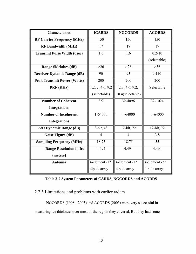
Considerable improvement in sidelobe levels, dynamic range and layering
information was observed. ACORDS was quite successful in mapping the bedrock
over most of the region covered by it. But it was unsuccessful in mapping outlet
glaciers in southern Greenland. Table (2.2) summarizes the system parameters of
ICARDS, NGCORDS and ACORDS [5,6 and 11].
12
Characteristics ICARDS NGCORDS ACORDS
RF Carrier Frequency (MHz) 150 150 150
RF Bandwidth (MHz) 17 17 17
Transmit Pulse Width (usec) 1.6 1.6 0.2-10
(selectable)
Range Sidelobes (dB) >26 >26 >36
Receiver Dynamic Range (dB) 90 93 >110
Peak Transmit Power (Watts) 200 200 200
PRF (KHz) 1.2, 2, 4.6, 9.2
(selectable)
2.3, 4.6, 9.2,
18.4(selectable)
Selectable
Number of Coherent
Integrations
??? 32-4096 32-1024
Number of Incoherent
Integrations
1-64000 1-64000 1-64000
A/D Dynamic Range (dB) 8-bit, 48 12-bit, 72 12-bit, 72
Noise Figure (dB) 4 4 3.8
Sampling Frequency (MHz) 18.75 18.75 55
Range Resolution in Ice
(meters)
4.494 4.494 4.494
Antenna 4-element λ/2
dipole array
4-element λ/2
dipole array
4-element λ/2
dipole array
Table 2-2 System Parameters of CARDS, NGCORDS and ACORDS
2.2.3 Limitations and problems with earlier radars
NGCORDS (1998 - 2003) and ACORDS (2003) were very successful in
measuring ice thickness over most of the region they covered. But they had some
13

limitations and there was quite a bit of scope for improvement. Given below is a
summarized list of limitations of NGCORDS and ACORDS
2.2.3.1 NGCORDS
Radar had to be operated over a limited frequency range, restricting the
accurate measurement of scattering properties in ice and basal conditions
Higher range sidelobes
Lower receiver dynamic range
Analog compression techniques introducing nonlinearities
Time varying gain control, making it tough to keep track of returned
signal power
Mixers used in down conversion to IF introduced nonlinearities
Entire radar and its power supply placed inside a huge rack mount chassis,
which made the system heavy, big and bulky
Poor range resolution of 4.494m, limiting the ability to accurately map the
deep internal layers
Radar had to be operated over limited frequencies and bandwidth
2.2.3.2 ACORDS
Radar had to be operated over limited frequency range restricting the
accurate measurement of scattering properties in ice and basal conditions
Poor range resolution of 4.494 m limiting the ability to accurately map
deeper internal layers
14
Radar had to be operated over limited frequencies and bandwidth
Uneven and larger than ideal sidelobe levels caused due to amplitude and
phase nonlinearities
Used many control and power lines, making the system messy
Though NGCORDS and ACORDS used surface mount components, each
module in the radar had to be placed inside an RF-shielded enclosure to
avoid coupling. All the modules and AC-DC power supply were placed
inside a huge rack mount chassis, which made the system heavy, big and
bulky
Sampling a 20-MHz bandwidth signal at 55 MHz provides very little
guard band and allow noise to couple into the signal band
2.2.4 Advantages and improvements with the Wide Band Depth Coherent
Radar Depth Sounder (WCORDS)
A Wideband Coherent Radar Depth Sounder (WCORDS) was developed to
solve the limitations of existing radars and improve upon them. The radar developed
would be able to operate over a partial or entire band from 50 MHz to 200 MHz.
Operating the radar over the entire bandwidth would considerably reduce the range
resolution to 55.9 cm, providing an accurate measure of deeper internal layers and
basal properties. Scattering properties in ice over two octaves could be obtained.
Operating the radar at lower frequency and wider bandwidth would probably reduce
off-vertical surface clutter and obtain better data over outlet glaciers in southern
15

Greenland. The radar would be considerably miniaturized to fit inside compact PCI
cards that would be placed inside a euro cage. Mounting the radar on a compact PCI
chassis would improve grounding between various modules. WCORDS would have
the following features
Frequency of operation between 50 MHz and 200 MHz
Amplitude and phase corrected transmit signal generated by an AWG
Received data sampled at very high frequency (500MHz) in the DAC
Dual channels in the receiver providing very high dynamic range
Small and compact
Eliminating limiter (surface-based applications) by providing a high-
power and high-speed receiver blanking switch
Including programmable CPLDs in the radar modules to reduce the
number of control lines and also simplify the method of varying radar
parameters
16

Chapter 3
Ice Sheet Model and System Parameters
3.1 Introduction
Chapters 1 and 2 discussed previously developed radars and requirements for
WCORDS. Chapter 3 describes a basic ice sheet model and its properties. The effects
of temperature, density, acidity and scattering on signal attenuation are discussed. Ice
loss over a wide range of frequencies is calculated using NGRIP temperature and
density profile data to obtain an accurate estimate of signal attenuation over the
operating frequency band. Receiver gain and other important radar parameters are
calculated in the later portion of the chapter.
3.2 Ice sheet model
As depicted in the figure, the top of the ice sheet is covered with a thin layer of snow,
beneath which is ice that can be as thick as 4km. A very thin layer of water could be
present between the ice and the bedrock. When a wave impinges on an interface
between two media, the difference between the amplitude of reflected and transmitted
signals depends on the ratio of dielectric constants of the two media. Thus, the
amplitude of signal reflected from air-ice interface or ice-bedrock interface is larger
17
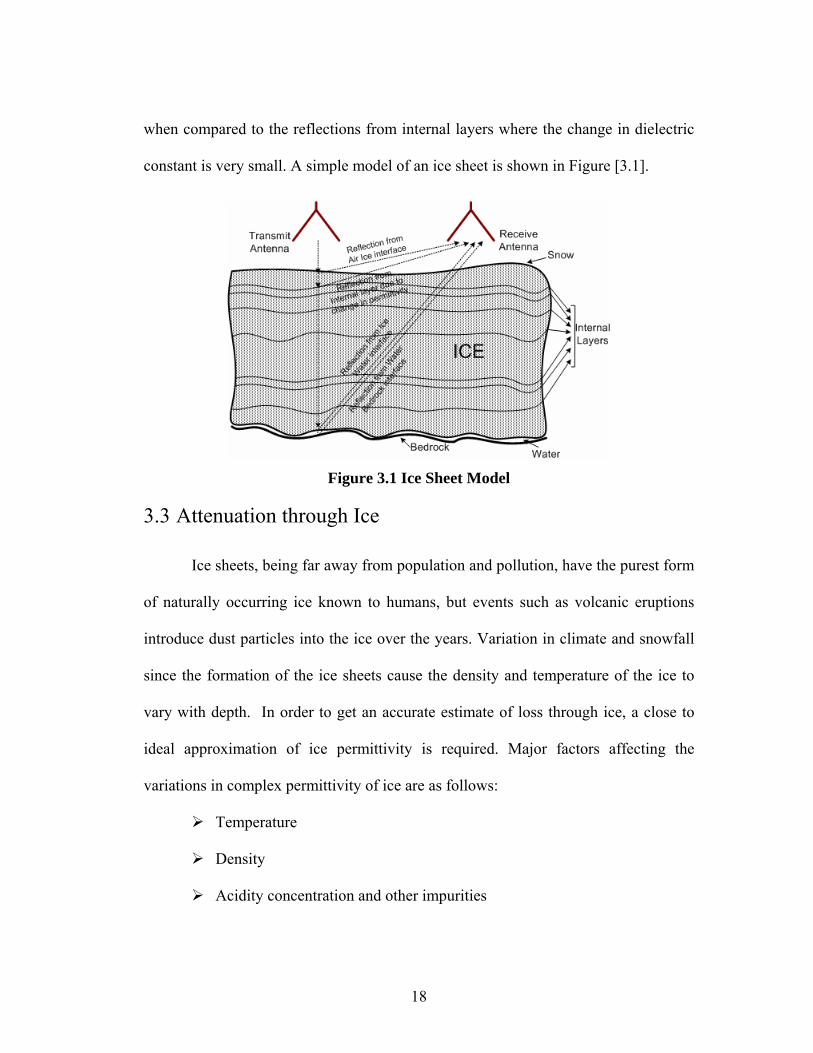
when compared to the reflections from internal layers where the change in dielectric
constant is very small. A simple model of an ice sheet is shown in Figure [3.1].
Figure 3.1 Ice Sheet Model
3.3 Attenuation through Ice
Ice sheets, being far away from population and pollution, have the purest form
of naturally occurring ice known to humans, but events such as volcanic eruptions
introduce dust particles into the ice over the years. Variation in climate and snowfall
since the formation of the ice sheets cause the density and temperature of the ice to
vary with depth. In order to get an accurate estimate of loss through ice, a close to
ideal approximation of ice permittivity is required. Major factors affecting the
variations in complex permittivity of ice are as follows:
Temperature
Density
Acidity concentration and other impurities
18

This subsection deals with the estimation of attenuation through ice at NGRIP.
Wave equation for a source free media is given as [24]
022 =+∇ ii EkE .,, zyxi= (3.1)
Where wave number of the medium ( )( )'''0 εεωσωµ jjjk −+−= 1−m
0µ =Permeability of free space = henrys/m 7104 −×π
''' εε j− =Permittivity of the medium
σ = Conductivity of the medium
Considering electric field polarized in x direction
Λ
= xx azEE )( (3.2)
Solving equation in
022
2
=+ xx Ek
dzEd (3.3)
Possible solution for the above homogeneous differential equation is given by,
[24]
γγ zx
zxx eEeEzE +−−+ += 00)( (3.4)
Where ( )( )'''0 εεωσωµγ jjjjk −+==
From equation 3.4, accurate knowledge of complex permittivity and
conductivity of the medium will enable us to calculate the signal attenuation in ice
over various frequencies at constant depth or vice versa.
19
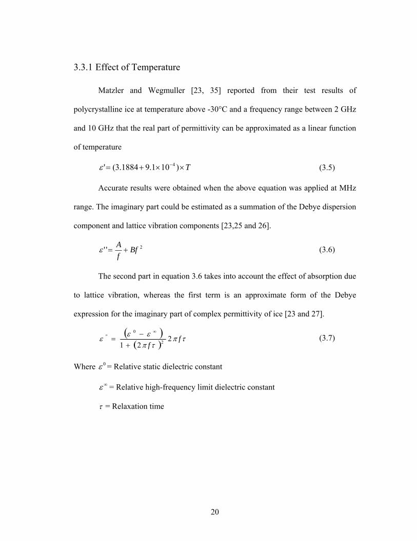
3.3.1 Effect of Temperature
Matzler and Wegmuller [23, 35] reported from their test results of
polycrystalline ice at temperature above -30°C and a frequency range between 2 GHz
and 10 GHz that the real part of permittivity can be approximated as a linear function
of temperature
T××+= − )101.91884.3(' 4ε (3.5)
Accurate results were obtained when the above equation was applied at MHz
range. The imaginary part could be estimated as a summation of the Debye dispersion
component and lattice vibration components [23,25 and 26].
2'' BffA+=ε (3.6)
The second part in equation 3.6 takes into account the effect of absorption due
to lattice vibration, whereas the first term is an approximate form of the Debye
expression for the imaginary part of complex permittivity of ice [23 and 27].
( )( )
τπτπ
εεε ff
221 2
0"
+−
=∞
(3.7)
Where = Relative static dielectric constant 0ε
∞ε = Relative high-frequency limit dielectric constant
τ = Relaxation time
20
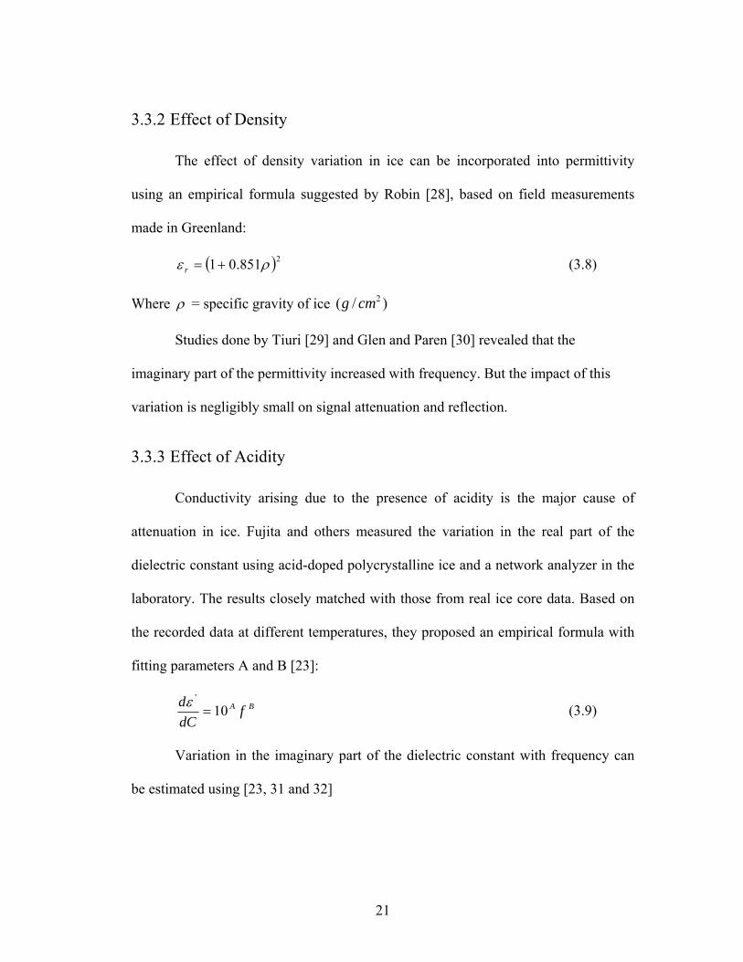
3.3.2 Effect of Density
The effect of density variation in ice can be incorporated into permittivity
using an empirical formula suggested by Robin [28], based on field measurements
made in Greenland:
( 2851.01 ρε +=r ) (3.8)
Where ρ = specific gravity of ice )/( 2cmg
Studies done by Tiuri [29] and Glen and Paren [30] revealed that the
imaginary part of the permittivity increased with frequency. But the impact of this
variation is negligibly small on signal attenuation and reflection.
3.3.3 Effect of Acidity
Conductivity arising due to the presence of acidity is the major cause of
attenuation in ice. Fujita and others measured the variation in the real part of the
dielectric constant using acid-doped polycrystalline ice and a network analyzer in the
laboratory. The results closely matched with those from real ice core data. Based on
the recorded data at different temperatures, they proposed an empirical formula with
fitting parameters A and B [23]:
BA fdCd 10
'
=ε (3.9)
Variation in the imaginary part of the dielectric constant with frequency can
be estimated using [23, 31 and 32]
21
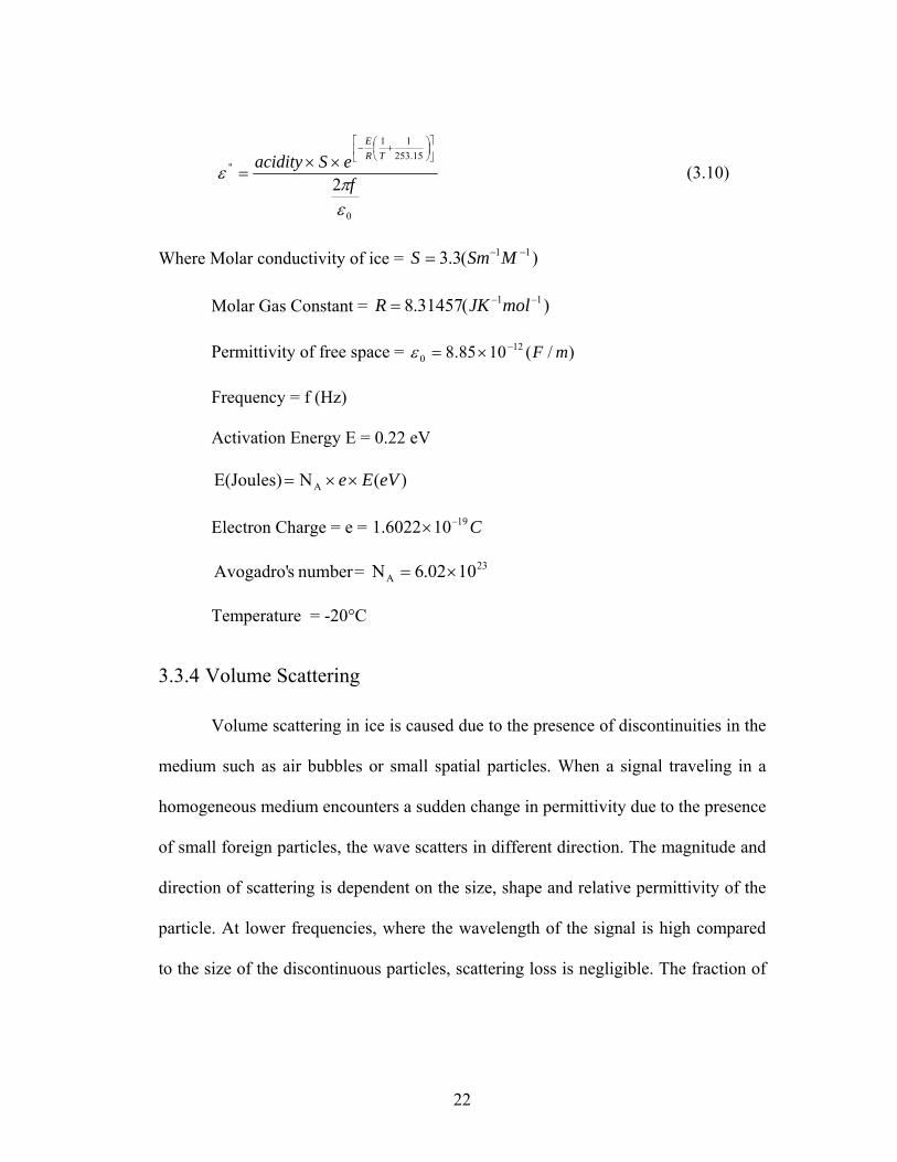
0
15.25311
''
2επ
εf
eSacidity TRE
⎥⎦
⎤⎢⎣
⎡⎟⎠⎞
⎜⎝⎛ +−
××= (3.10)
Where Molar conductivity of ice = )(3.3 11 −−= MSmS
Molar Gas Constant = )(31457.8 11 −−= molJKR
Permittivity of free space = )/(1085.8 120 mF−×=ε
Frequency = f (Hz)
Activation Energy E = 0.22 eV
)(NE(Joules) A eVEe××=
Electron Charge = e = C19106022.1 −×
number sAvogadro' = 23A 1002.6N ×=
Temperature = -20°C
3.3.4 Volume Scattering
Volume scattering in ice is caused due to the presence of discontinuities in the
medium such as air bubbles or small spatial particles. When a signal traveling in a
homogeneous medium encounters a sudden change in permittivity due to the presence
of small foreign particles, the wave scatters in different direction. The magnitude and
direction of scattering is dependent on the size, shape and relative permittivity of the
particle. At lower frequencies, where the wavelength of the signal is high compared
to the size of the discontinuous particles, scattering loss is negligible. The fraction of
22
power lost due to the presence of spherical discontinuous particles in the medium is
given by [33 and 34]:
2
21
212
4
0
6
2)(2
38
⎥⎦
⎤⎢⎣
⎡+−
⎟⎟⎠
⎞⎜⎜⎝
⎛=
εεεεε
λππδ mb (3.11)
Where m = Number of particles per unit volume
b = Radius of the particles
1ε = Permittivity of the particle
2ε = Permittivity of the medium
Consider a case where spherical bubbles with a 1 mm radius are trapped
inside a continuous medium of ice. Attenuation due to scattering can be derived from
equation 3.11 [33] to be equal to:
dBL 40
4105λ
−×= per 100m (3.12)
At our highest frequency of operation (200 MHz), attenuation is calculated to
be equal to . This loss is negligibly small when compared to
loss due to other effects.
mdB 100/1077.98 6−×
Ice temperature and density profile data are available from the NGRIP drill
site [31]. Though the data are not available down to the bedrock (3085 m),
interpolating the available data will provide a close approximation of ideal results.
Signal loss in ice due to temperature, density and acidity levels over a wide frequency
band is plotted in Figure [3.2].
23
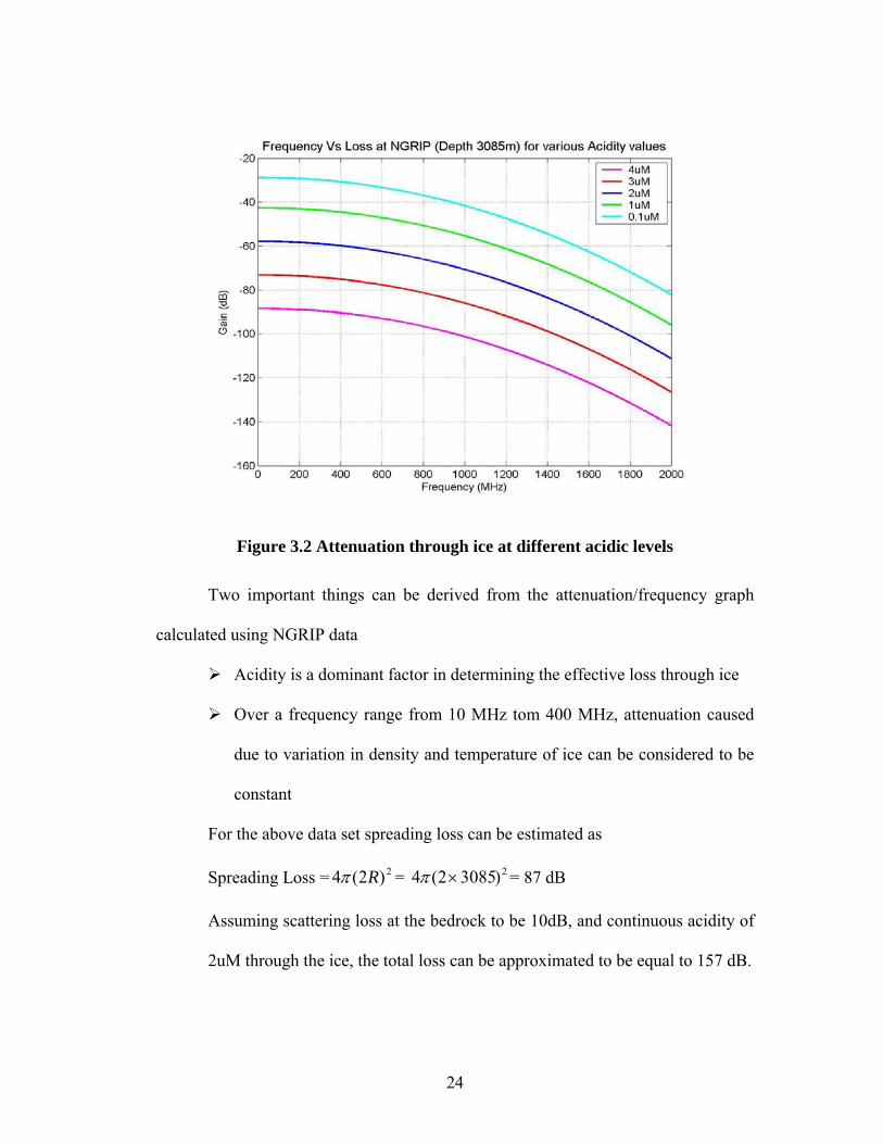
Figure 3.2 Attenuation through ice at different acidic levels
Two important things can be derived from the attenuation/frequency graph
calculated using NGRIP data
Acidity is a dominant factor in determining the effective loss through ice
Over a frequency range from 10 MHz tom 400 MHz, attenuation caused
due to variation in density and temperature of ice can be considered to be
constant
For the above data set spreading loss can be estimated as
Spreading Loss = = = 87 dB 2)2(4 Rπ 2)30852(4 ×π
Assuming scattering loss at the bedrock to be 10dB, and continuous acidity of
2uM through the ice, the total loss can be approximated to be equal to 157 dB.
24
3.4 Derivation of system specifications
Ideally, radar should be able to obtain all the required information about the
target while transmitting a minimum amount of power. WCORDS is required to
detect and differentiate multiple targets in the form of internal layers, top and
bedrock. The amount of power reflected back form each of these targets primarily
depends on the distance of the target from the source and the difference in dielectric
constant between the layers. The dynamic range of the radar receiver should be large
enough to record the high amplitude reflected signal from the top and shallow internal
layers and also the very low amplitude reflection from the bedrock, which is at least
4km deep. A large dynamic range in the receiver can be achieved either by
incorporating time varying gain into the receiver or splitting the receiver into multiple
gain channels. Time-varying gain of the receiver introduces an element of error in
estimating accurately the return signal power from each layer. Introduction of
multiple channels in the receiver provides improvement in the dynamic range of the
receiver and allows better control over overall receiver gain at the expense of multiple
data acquisition systems.
From the previous section, the total loss through 3085-m ice at NGRIP was
calculated to be close to 150 dB. In order to overcome such a huge ice loss, the radar
would be required to have very large loop sensitivity, which can be achieved by
transmitting a very large signal and/or designing a sensitive receiver. Some of the
limitations encountered when transmitting high power signals are:
Large power consumption
25

High power amplifiers are costly, big and bulky
Power amplifiers are limited by turn-on and turn-off times thereby
restricting the radar to operate at narrow pulse widths
Transmitting high power would require the transmitter and receiver antennas
to be placed far apart to prevent the direct feed through signal from
damaging the receiver
Generally, a high-power amplifier generates large harmonics and spurious
signals which might interfere with other communication systems operating
in close vicinity
Baluns or other impedance transformation devices used for antenna
matching are big in size, costly and tough to manufacture when operated at
high power
Hence, an optimum solution would be to design a sensitive receiver using a
minimal amount of transmit power to obtain the required signal-to-noise ratio.
Depending on the mode, bandwidth and characteristics of ice in the region of
operation, the transmit power can be varied to get optimum performance. Post
processing techniques such as coherent and incoherent integrations can be used to
improve the signal quality. Gain required in both the gain channels depends on
system parameters such as receiver noise, Analog to Digital Converter (ADC) noise
level and signal processing gain.
26
3.4.1.1 System parameters
3..4.1.1.1 Receiver Noise Floor
The amplitude of receiver noise floor is equal to the product of thermal noise
and receiver noise figure:
)()()( Re dBNFdBmNdBN ceiverThermalSystem += (3.13)
Where Thermal Noise KTBNThermal = (Noise power at the antenna)
Boltzman Constant deg/1038.1 23 JK −×=
Equivalent Noise Temperature KT 290=
System Bandwidth MHzB 150=
dBmWKTBNThermal 21.92103.600 15 −=×== − (3.14)
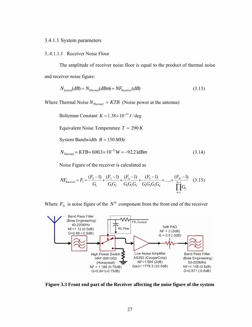
Noise Figure of the receiver is calculated as
∏−
=
−++
−+
−+
−+
−+= 1
1
4321
5
321
4
21
3
1
21Re
)1(.....
)1()1()1()1(N
kk
Nceiver
G
FGGGG
FGGG
FGG
FG
FFNF (3.15)
Where is noise figure of the component from the front end of the receiver NF thN
Figure 3.3 Front end part of the Receiver affecting the noise figure of the system
27
....5.04.1778841.089.0
)1148.1(4.1778841.089.0
)12(841.089.0
)1584.1(89.0
)1188.1(12.1Re +×××
−+
××−
+×−
+−
+=ceiverNF
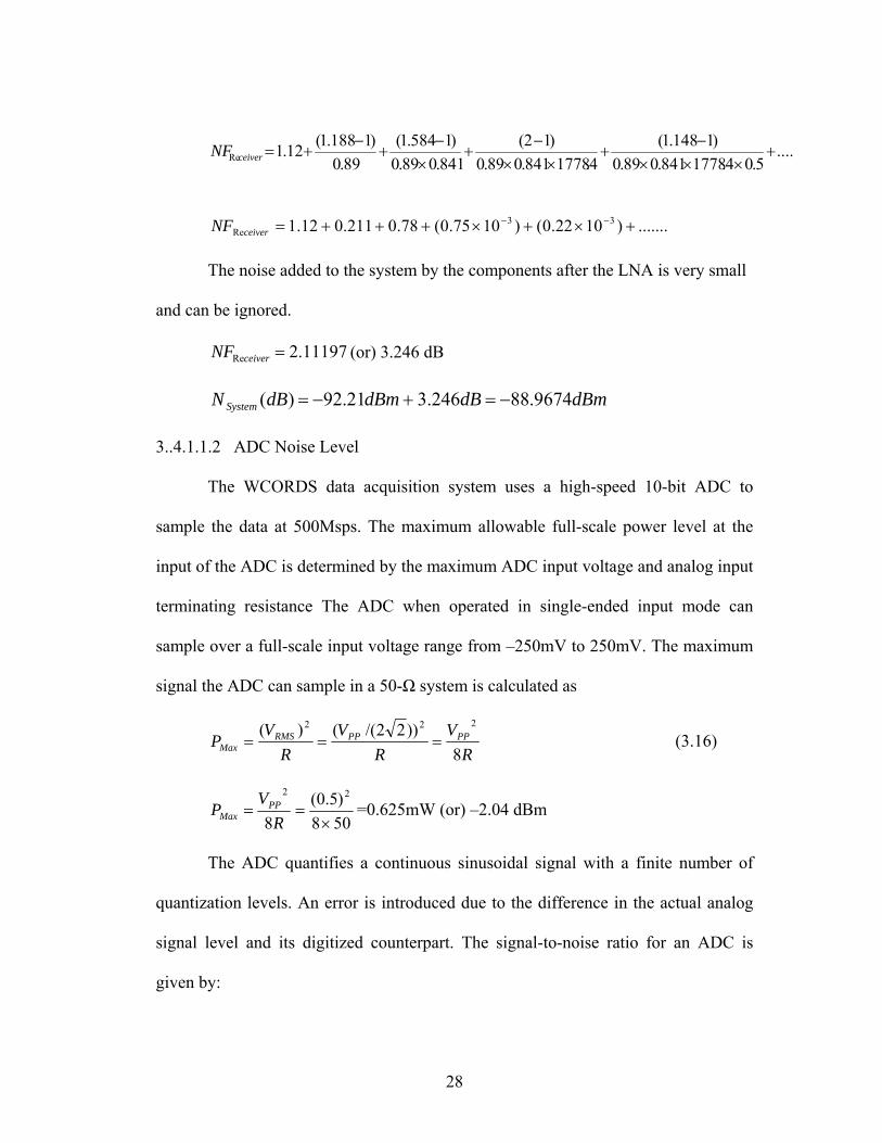
.......)1022.0()1075.0(78.0211.012.1 33Re +×+×+++= −−
ceiverNF
The noise added to the system by the components after the LNA is very small
and can be ignored.
11197.2Re =ceiverNF (or) 3.246 dB
dBmdBdBmdBN System 9674.88246.321.92)( −=+−=
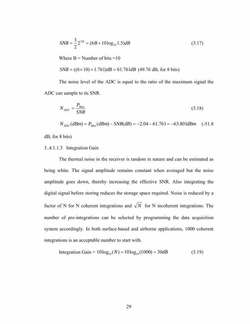
3..4.1.1.2 ADC Noise Level
The WCORDS data acquisition system uses a high-speed 10-bit ADC to
sample the data at 500Msps. The maximum allowable full-scale power level at the
input of the ADC is determined by the maximum ADC input voltage and analog input
terminating resistance The ADC when operated in single-ended input mode can
sample over a full-scale input voltage range from –250mV to 250mV. The maximum
signal the ADC can sample in a 50-Ω system is calculated as
RV
RV
RV
P PPPPRMSMax 8
))22/(()( 222
=== (3.16)
508)5.0(
8
22
×==
RVP PP
Max =0.625mW (or) –2.04 dBm
The ADC quantifies a continuous sinusoidal signal with a finite number of
quantization levels. An error is introduced due to the difference in the actual analog
signal level and its digitized counterpart. The signal-to-noise ratio for an ADC is
given by:
28
dBBSNR B )5.1log106(223
102 +== (3.17)
Where B = Number of bits =10
dBdBSNR 761.61)761.1)106(( =+×= (49.76 dB, for 8 bits)
The noise level of the ADC is equal to the ratio of the maximum signal the
ADC can sample to its SNR.
SNRP
N MaxADC = (3.18)
dBmdBSNRdBmPdBmN MaxADC 801.63761.6104.2)()()( −=−−=−= (-51.8
dB, for 8 bits)
3..4.1.1.3 Integration Gain
The thermal noise in the receiver is random in nature and can be estimated as
being white. The signal amplitude remains constant when averaged but the noise
amplitude goes down, thereby increasing the effective SNR. Also integrating the
digital signal before storing reduces the storage space required. Noise is reduced by a
factor of N for N coherent integrations and N for N incoherent integrations. The
number of pre-integrations can be selected by programming the data acquisition
system accordingly. In both surface-based and airborne applications, 1000 coherent
integrations is an acceptable number to start with.
Integration Gain = dBN 30)1000(log10)(log10 1010 == (3.19)
29
3..4.1.1.4 Pulse Compression Gain
Digital pulse compression using a match-filtering technique provides
compression gain in post processing. The compression gain is equal to the product of
the bandwidth and the transmit pulse width.
BTPCG = (3.20)
)(log10)( 10 BTdBPCG = (3.21)
Where B =Bandwidth =150 MHz
T = Transmit pulse width
For a 1usec pulse width, compression gain of 21.761 dB is obtained
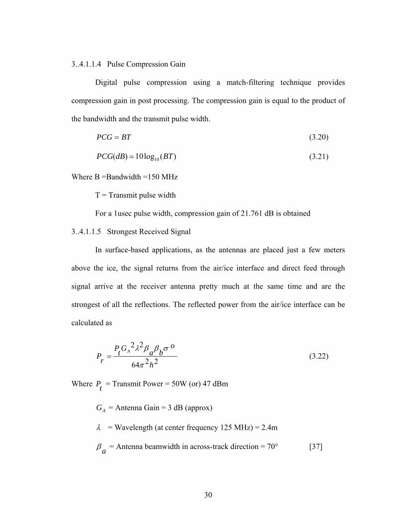
3..4.1.1.5 Strongest Received Signal
In surface-based applications, as the antennas are placed just a few meters
above the ice, the signal returns from the air/ice interface and direct feed through
signal arrive at the receiver antenna pretty much at the same time and are the
strongest of all the reflections. The reflected power from the air/ice interface can be
calculated as
2264
22
h
obaGtP
rPA
π
σββλ= (3.22)
Where = Transmit Power = 50W (or) 47 dBm tP
AG = Antenna Gain = 3 dB (approx)
λ = Wavelength (at center frequency 125 MHz) = 2.4m
aβ = Antenna beamwidth in across-track direction = 70° [37]
30
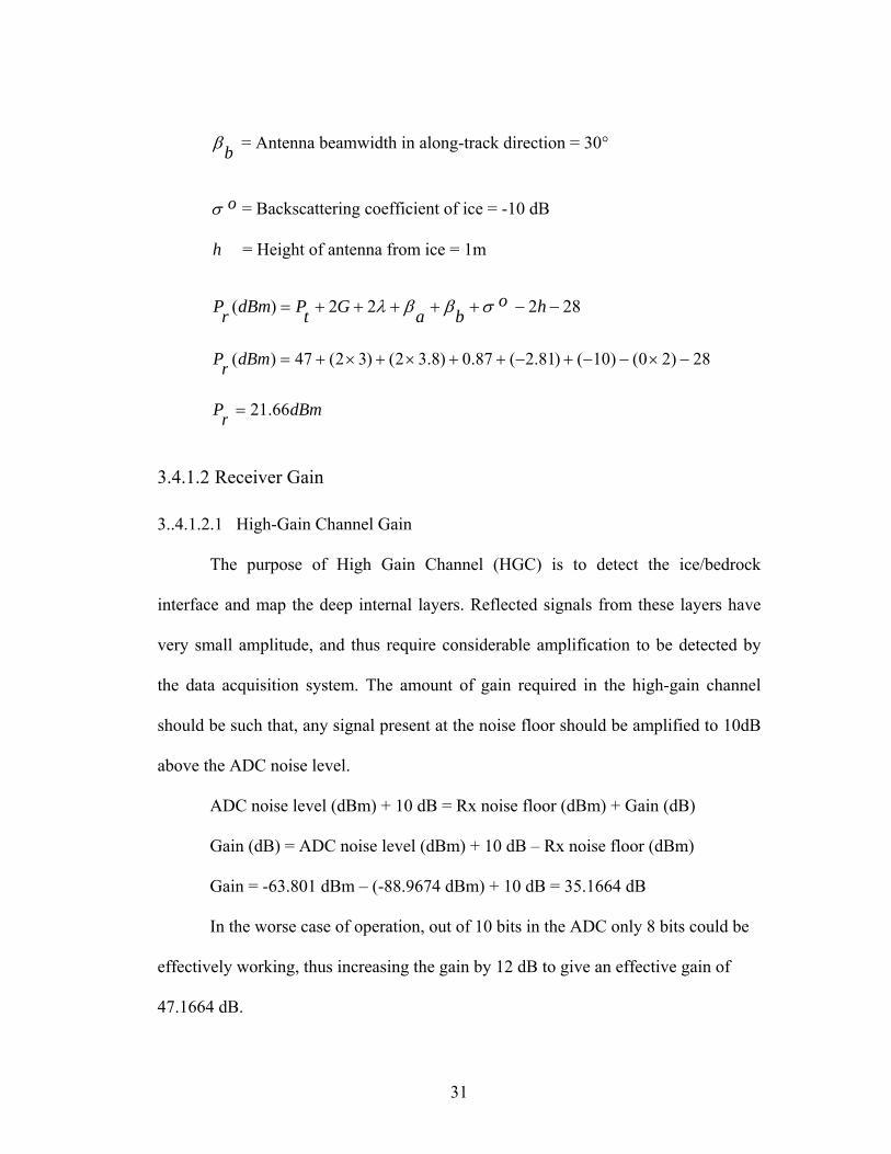
bβ = Antenna beamwidth in along-track direction = 30°
oσ = Backscattering coefficient of ice = -10 dB
h = Height of antenna from ice = 1m
28222)( −−+++++= hobaGtPdBmrP σββλ
28)20()10()81.2(87.0)8.32()32(47)( −×−−+−++×+×+=dBmrP
dBmrP 66.21=
3.4.1.2 Receiver Gain
3..4.1.2.1 High-Gain Channel Gain
The purpose of High Gain Channel (HGC) is to detect the ice/bedrock
interface and map the deep internal layers. Reflected signals from these layers have
very small amplitude, and thus require considerable amplification to be detected by
the data acquisition system. The amount of gain required in the high-gain channel
should be such that, any signal present at the noise floor should be amplified to 10dB
above the ADC noise level.
ADC noise level (dBm) + 10 dB = Rx noise floor (dBm) + Gain (dB)
Gain (dB) = ADC noise level (dBm) + 10 dB – Rx noise floor (dBm)
Gain = -63.801 dBm – (-88.9674 dBm) + 10 dB = 35.1664 dB
In the worse case of operation, out of 10 bits in the ADC only 8 bits could be
effectively working, thus increasing the gain by 12 dB to give an effective gain of
47.1664 dB.
31
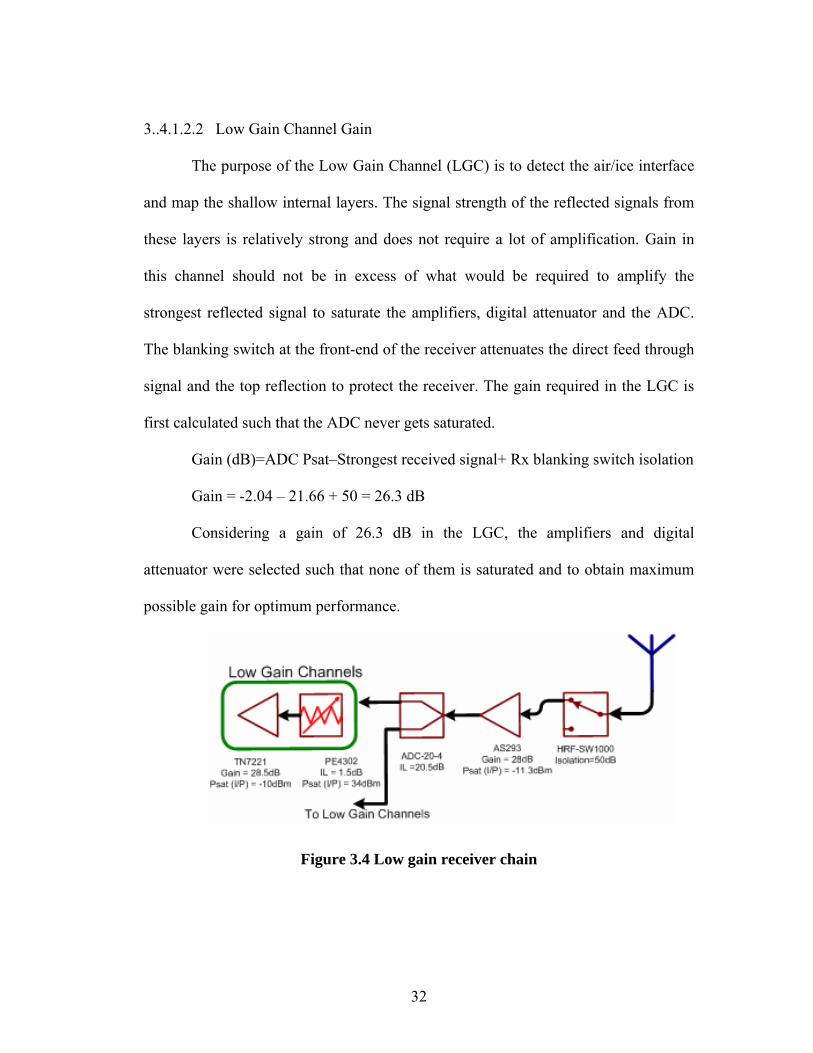
3..4.1.2.2 Low Gain Channel Gain
The purpose of the Low Gain Channel (LGC) is to detect the air/ice interface
and map the shallow internal layers. The signal strength of the reflected signals from
these layers is relatively strong and does not require a lot of amplification. Gain in
this channel should not be in excess of what would be required to amplify the
strongest reflected signal to saturate the amplifiers, digital attenuator and the ADC.
The blanking switch at the front-end of the receiver attenuates the direct feed through
signal and the top reflection to protect the receiver. The gain required in the LGC is
first calculated such that the ADC never gets saturated.
Gain (dB)=ADC Psat–Strongest received signal+ Rx blanking switch isolation
Gain = -2.04 – 21.66 + 50 = 26.3 dB
Considering a gain of 26.3 dB in the LGC, the amplifiers and digital
attenuator were selected such that none of them is saturated and to obtain maximum
possible gain for optimum performance.
Figure 3.4 Low gain receiver chain
32
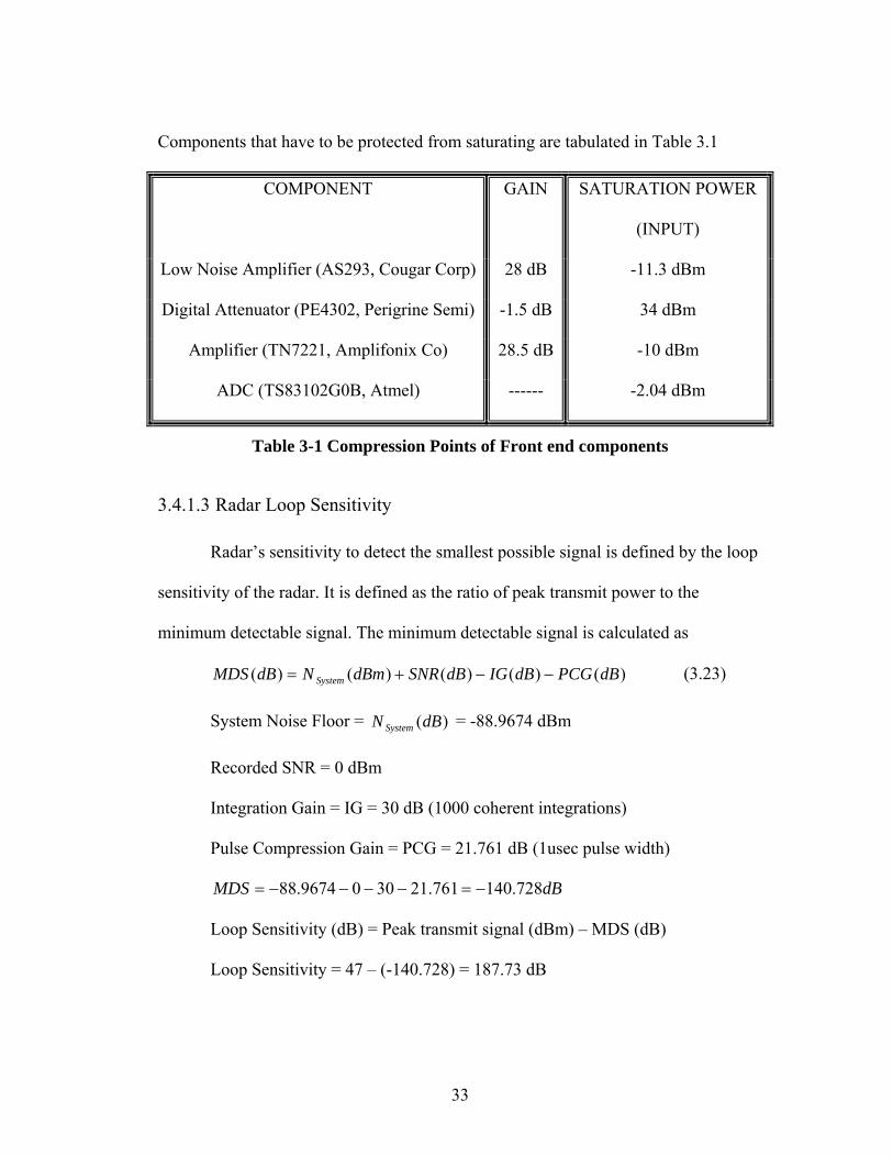
Components that have to be protected from saturating are tabulated in Table 3.1
COMPONENT GAIN SATURATION POWER
(INPUT)
Low Noise Amplifier (AS293, Cougar Corp) 28 dB -11.3 dBm
Digital Attenuator (PE4302, Perigrine Semi) -1.5 dB 34 dBm
Amplifier (TN7221, Amplifonix Co) 28.5 dB -10 dBm
ADC (TS83102G0B, Atmel) ------ -2.04 dBm
Table 3-1 Compression Points of Front end components
3.4.1.3 Radar Loop Sensitivity
Radar’s sensitivity to detect the smallest possible signal is defined by the loop
sensitivity of the radar. It is defined as the ratio of peak transmit power to the
minimum detectable signal. The minimum detectable signal is calculated as
)()()()()( dBPCGdBIGdBSNRdBmNdBMDS System −−+= (3.23)
System Noise Floor = = -88.9674 dBm )(dBN System
Recorded SNR = 0 dBm
Integration Gain = IG = 30 dB (1000 coherent integrations)
Pulse Compression Gain = PCG = 21.761 dB (1usec pulse width)
dBMDS 728.140761.213009674.88 −=−−−−=
Loop Sensitivity (dB) = Peak transmit signal (dBm) – MDS (dB)
Loop Sensitivity = 47 – (-140.728) = 187.73 dB
33

Chapter 4
Wideband Coherent Radar Depth Sounder
4.1 System overview and operation
WCORDS is a frequency chirped pulse radar operating in the VHF and UHF
bands to measure ice sheet thickness up to a depth of 4km and map deeper internal
layers with a fine resolution of 56 cm. Basal properties and scattering characteristics
can be obtained from the recorded data. The radar is designed to operate in both
surface-based and airborne applications. Capturing the data directly enables the radar
to be operated in chirp and step-frequency modes. A detailed block diagram of
WCORDS is shown in Figure (4.1); the un-shaded region in the block diagram is the
analog part of the radar.
4.1.1 Transmitter
A highly stable, 10-MHz Rubidium reference oscillator with very low phase
noise drives all the control and timing signals in the system. The transmit chirp signal
of 50-200 MHz is generated using an AWG with selectable pulse widths. The
frequency synthesizer provides a 500-MHz signal, which is phase locked to the 10-
MHz reference oscillator. The AWG uses the phase-locked 500-MHz synthesizer
signal as the clock signal to generate the 50-200-MHz chirp signal. Triggering and
34

control signals to determine the pulse repetition frequency (PRF), signal amplitude
and other AWG characteristics are generated by the control unit that runs off the 10-
MHz reference oscillator. The chirp signal is filtered for any unwanted noise signals
generated by the AWG and then amplified to the optimum signal level by the
transmitter module. The transmitter blanking switch provides better control over the
signal pulse width and filters out any unwanted signals generated outside the
transmitted pulse by the AWG. Combined reverse isolation of amplifiers and the
transmitter blanking switch protect the transmitter and AWG from any unexpected
high amplitude signals picked up by the transmitter antenna.
Figure 4.1 WCORDS Block diagram
35
4.1.2 Receiver
A high power receiver-blanking switch protects the receiver from the large
direct feed through signal and reflections from the top and near-surface internal
layers. The receiver consists of dual gain channels to obtain a high dynamic range.
The high-gain blanking switch protects the high-gain channel from saturation and
damaging while receiving large reflected signals. Digital attenuators provide gain
adjustment in the receiver to obtain optimum performance under various working
conditions. The digital system generates the control signals for all the blanking
switches and digital attenuators. High-speed, 10-bit ADC sample the analog signal at
500 MHz. A de-multiplexer after the ADC slows the data rate by 4 times to make it
easier to record and work with the data. The number of coherent and incoherent
integrations, switching timing controls and digital attenuator bit vales are selectable
and easily programmable. The high-speed data acquisitions system and digital control
unit were designed and developed by Mr. Torry Akins.
The radar can be operated in between the range or entirely over a wide
frequency band of 50 MHz to 200 MHz. In a noisy environment, the radar can be
operated in step-frequency mode or over a selective bandwidth by just including
external additional bandpass filters at the receiver input. The number of coherent and
incoherent averages practically possible depend on the operational PRF,
characteristics of ice (ice thickness, scattering characteristics, etc) in that region and
the velocity of the vehicle on which the radar is mounted. Important WCORDS
system parameters are tabulated in Table (4.1).
36
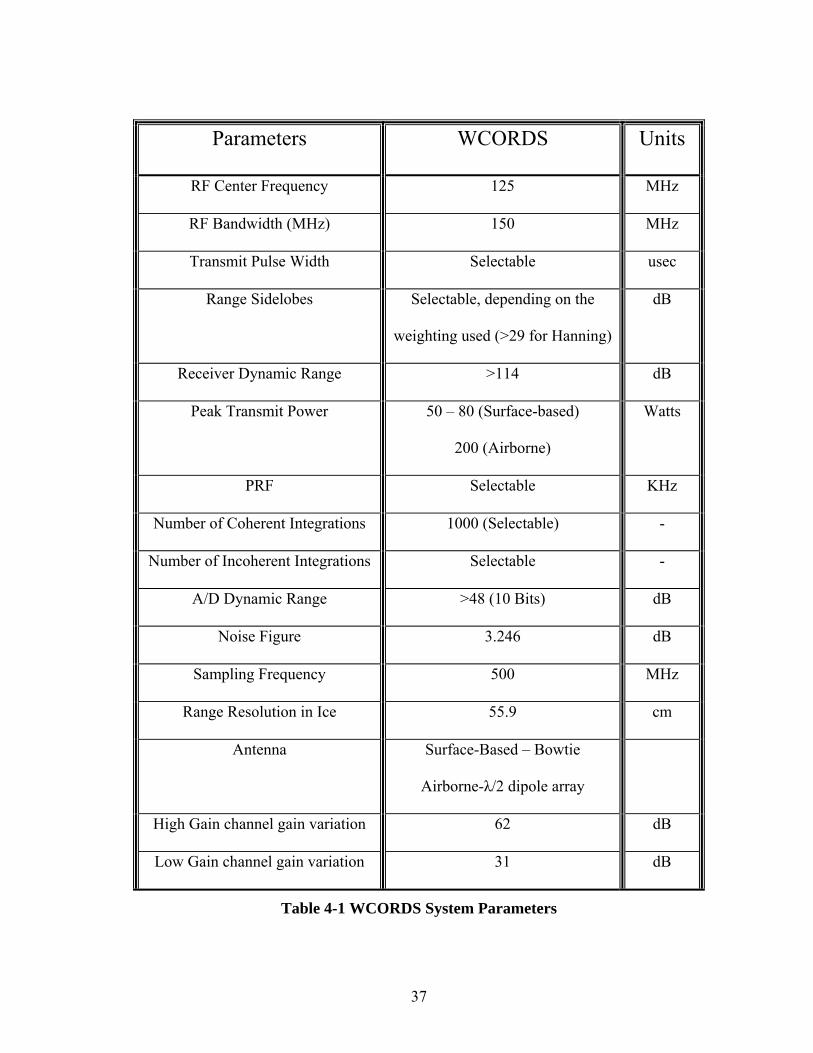
Parameters WCORDS Units
RF Center Frequency 125 MHz
RF Bandwidth (MHz) 150 MHz
Transmit Pulse Width Selectable usec
Range Sidelobes Selectable, depending on the
weighting used (>29 for Hanning)
dB
Receiver Dynamic Range >114 dB
Peak Transmit Power 50 – 80 (Surface-based)
200 (Airborne)
Watts
PRF Selectable KHz
Number of Coherent Integrations 1000 (Selectable) -
Number of Incoherent Integrations Selectable -
A/D Dynamic Range >48 (10 Bits) dB
Noise Figure 3.246 dB
Sampling Frequency 500 MHz
Range Resolution in Ice 55.9 cm
Antenna Surface-Based – Bowtie
Airborne-λ/2 dipole array
High Gain channel gain variation 62 dB
Low Gain channel gain variation 31 dB
Table 4-1 WCORDS System Parameters
37
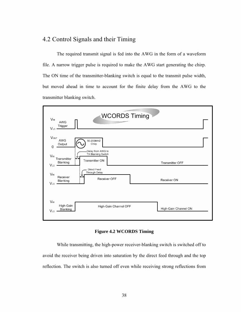
4.2 Control Signals and their Timing
The required transmit signal is fed into the AWG in the form of a waveform
file. A narrow trigger pulse is required to make the AWG start generating the chirp.
The ON time of the transmitter-blanking switch is equal to the transmit pulse width,
but moved ahead in time to account for the finite delay from the AWG to the
transmitter blanking switch.
Figure 4.2 WCORDS Timing
While transmitting, the high-power receiver-blanking switch is switched off to
avoid the receiver being driven into saturation by the direct feed through and the top
reflection. The switch is also turned off even while receiving strong reflections from
38
near-surface internal layers and it is switched on only when the received signal power
is just less that what would be required to saturate the LGC in the receiver. Similarly,
as long as the signal power is high enough to saturate the HGC, the High-Gain
blanking is switched off. As soon as the amplitude of the received signal level drops
to a point where it doesn’t saturate the HGC of the receiver any more, the High-Gain
blanking is switched on. Both the blanking switches used in the receiver are
absorptive and when switched off, they are terminated to ground through a 50-Ω
impedance to minimize the reflected signal power.
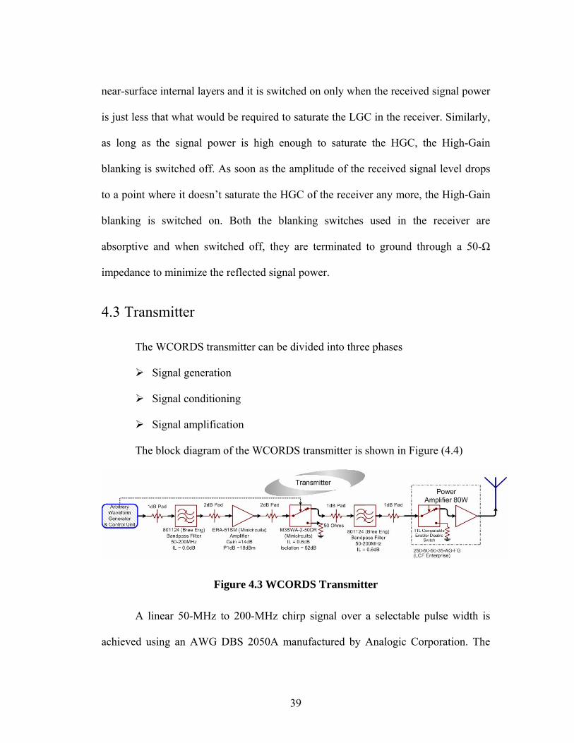
4.3 Transmitter
The WCORDS transmitter can be divided into three phases
Signal generation
Signal conditioning
Signal amplification
The block diagram of the WCORDS transmitter is shown in Figure (4.4)
Figure 4.3 WCORDS Transmitter
A linear 50-MHz to 200-MHz chirp signal over a selectable pulse width is
achieved using an AWG DBS 2050A manufactured by Analogic Corporation. The
39
required chirp waveform sampled at 500 MHz is generated using MATLAB and fed
into the AWG in the form of a waveform file. A compact waveform generator using a
Direct Digital Synthesizer (DDS) is being developed by Mr. Torry Akins to replace
the AWG. The AWG is immediately followed by a bandpass filter to remove any
unwanted out-of-band image frequencies, harmonics and other spurious signals that
might interfere with other communication and radar systems operating in the radar’s
close vicinity. After passing through the filter, the signal is pre-amplified with a low
power amplifier (Minicircuits ERA-51SM). The preamplifier was selected such that
the gain and output saturation point of the amplifier were sufficient to drive the power
amplifier to its maximum power. The preamplifier is followed by a single-pole-
double-throw (SPDT) switch (Minicircuits M3SWA-2-50DR) with high isolation to
reduce leakage signal. Even a small in-band signal generated by the waveform
generator lying outside the pulse will get amplified to a considerable power level
before being transmitted. Reflected signals from this transmitted leakage can be
mistaken for low power signal reflections of actual signal from deep internal layers.
The control signals for the high-isolation switch were setup such that the switch
would be ON during the transmit pulse duration and OFF during the rest of the time
period. Being an active component, the pre-amplifier and the switch would generate
harmonics and other spurious signals like inter-modulation products and switching
transients. A bandpass filter precedes the switch and preamplifier to remove any
spurious signals generated by them. After going through the conditioning phase and
pre-amplification, the signal is amplified to 50W (47 dBm) by a power amplifier
40
(LCF Enterprise 250-50-50-35-AG-FG). The power amplifier can be switched OFF
when not transmitting thus blocking any unwanted signals outside the pulse duration.
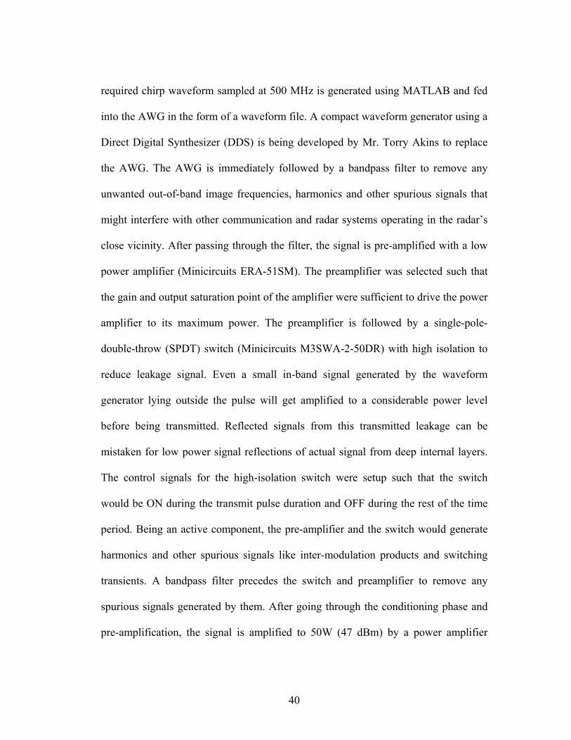
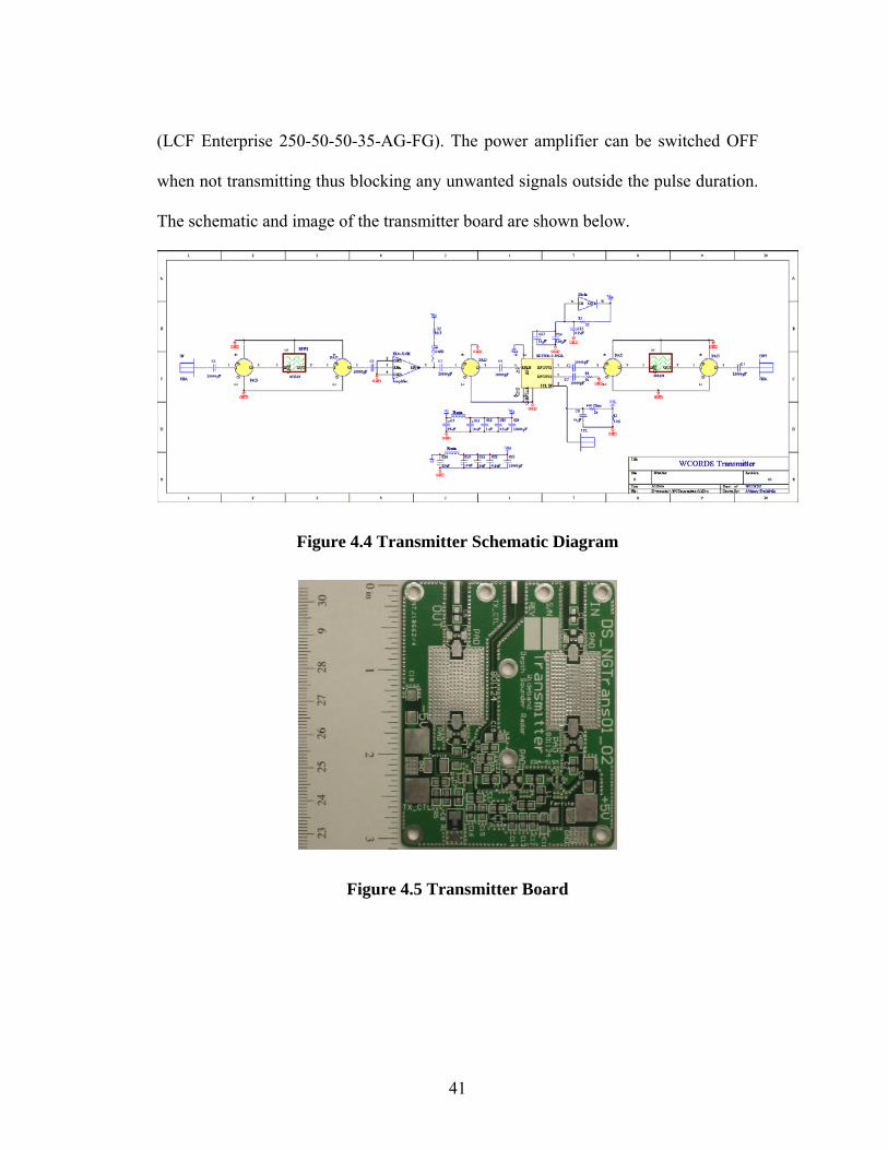
The schematic and image of the transmitter board are shown below.
Figure 4.4 Transmitter Schematic Diagram
Figure 4.5 Transmitter Board
41

4.4 Receiver
The design of the WCORDS receiver was based on the gain calculations
presented in Chapter 3, and given below is a summary of all the requirements that had
to be satisfied.
High dynamic range to detect both deep internal layers and bedrock
clearly
Effective gain in the HGC to be more than 48 dB
Effective gain in the LGC to be more than 32 dB
Minimum possible noise figure with optimum performance
Ability to vary the gain of the receiver over a wide range
Flat amplitude response and linear phase response over the entire band
Front-end of the receiver should have high input return loss, thus
minimizing the amplitude of signal reflected back through the transmitter
antenna to generate a multiple
Small and compact to fit into a single aluminum compact PCI card
Providing ease of control
The WCORDS receiver was divided into three modules to provide good
isolation and make the boards easy to design and debug for errors
Front-end module
Low Gain Channel
High Gain Channel
42
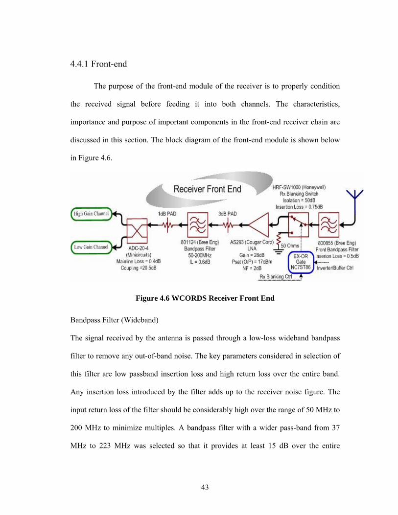
4.4.1 Front-end
The purpose of the front-end module of the receiver is to properly condition
the received signal before feeding it into both channels. The characteristics,
importance and purpose of important components in the front-end receiver chain are
discussed in this section. The block diagram of the front-end module is shown below
in Figure 4.6.
Figure 4.6 WCORDS Receiver Front End
Bandpass Filter (Wideband)
The signal received by the antenna is passed through a low-loss wideband bandpass
filter to remove any out-of-band noise. The key parameters considered in selection of
this filter are low passband insertion loss and high return loss over the entire band.
Any insertion loss introduced by the filter adds up to the receiver noise figure. The
input return loss of the filter should be considerably high over the range of 50 MHz to
200 MHz to minimize multiples. A bandpass filter with a wider pass-band from 37
MHz to 223 MHz was selected so that it provides at least 15 dB over the entire
43
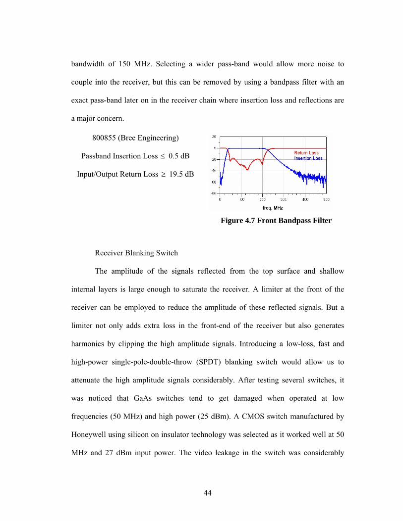
bandwidth of 150 MHz. Selecting a wider pass-band would allow more noise to
couple into the receiver, but this can be removed by using a bandpass filter with an
exact pass-band later on in the receiver chain where insertion loss and reflections are
a major concern.
800855 (Bree Engineering)
Passband Insertion Loss 0.5 dB ≤
Input/Output Return Loss ≥ 19.5 dB
Figure 4.7 Front Bandpass Filter
Receiver Blanking Switch
The amplitude of the signals reflected from the top surface and shallow
internal layers is large enough to saturate the receiver. A limiter at the front of the
receiver can be employed to reduce the amplitude of these reflected signals. But a
limiter not only adds extra loss in the front-end of the receiver but also generates
harmonics by clipping the high amplitude signals. Introducing a low-loss, fast and
high-power single-pole-double-throw (SPDT) blanking switch would allow us to
attenuate the high amplitude signals considerably. After testing several switches, it
was noticed that GaAs switches tend to get damaged when operated at low
frequencies (50 MHz) and high power (25 dBm). A CMOS switch manufactured by
Honeywell using silicon on insulator technology was selected as it worked well at 50
MHz and 27 dBm input power. The video leakage in the switch was considerably
44
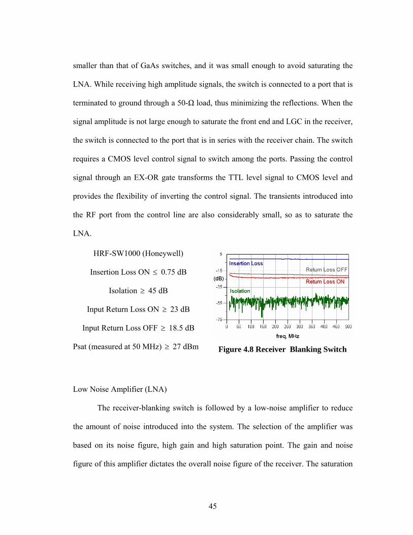
smaller than that of GaAs switches, and it was small enough to avoid saturating the
LNA. While receiving high amplitude signals, the switch is connected to a port that is
terminated to ground through a 50-Ω load, thus minimizing the reflections. When the
signal amplitude is not large enough to saturate the front end and LGC in the receiver,
the switch is connected to the port that is in series with the receiver chain. The switch
requires a CMOS level control signal to switch among the ports. Passing the control
signal through an EX-OR gate transforms the TTL level signal to CMOS level and
provides the flexibility of inverting the control signal. The transients introduced into
the RF port from the control line are also considerably small, so as to saturate the
LNA.
HRF-SW1000 (Honeywell)
Insertion Loss ON 0.75 dB ≤
Isolation ≥ 45 dB
Input Return Loss ON 23 dB ≥
Input Return Loss OFF 18.5 dB ≥
Psat (measured at 50 MHz) 27 dBm ≥
Figure 4.8 Receiver Blanking Switch
Low Noise Amplifier (LNA)
The receiver-blanking switch is followed by a low-noise amplifier to reduce
the amount of noise introduced into the system. The selection of the amplifier was
based on its noise figure, high gain and high saturation point. The gain and noise
figure of this amplifier dictates the overall noise figure of the receiver. The saturation
45
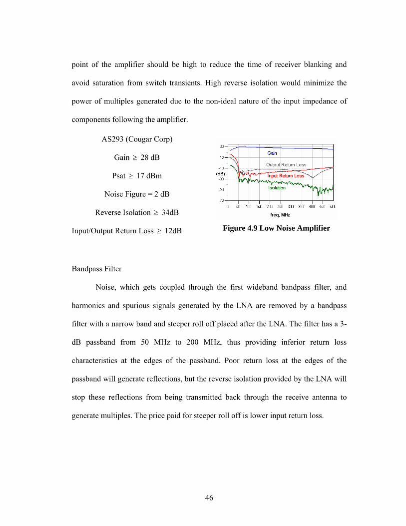
point of the amplifier should be high to reduce the time of receiver blanking and
avoid saturation from switch transients. High reverse isolation would minimize the
power of multiples generated due to the non-ideal nature of the input impedance of
components following the amplifier.
AS293 (Cougar Corp)
Gain ≥ 28 dB
Psat 17 dBm ≥
Noise Figure = 2 dB
Reverse Isolation 34dB ≥
Input/Output Return Loss 12dB ≥
Figure 4.9 Low Noise Amplifier
Bandpass Filter
Noise, which gets coupled through the first wideband bandpass filter, and
harmonics and spurious signals generated by the LNA are removed by a bandpass
filter with a narrow band and steeper roll off placed after the LNA. The filter has a 3-
dB passband from 50 MHz to 200 MHz, thus providing inferior return loss
characteristics at the edges of the passband. Poor return loss at the edges of the
passband will generate reflections, but the reverse isolation provided by the LNA will
stop these reflections from being transmitted back through the receive antenna to
generate multiples. The price paid for steeper roll off is lower input return loss.
46
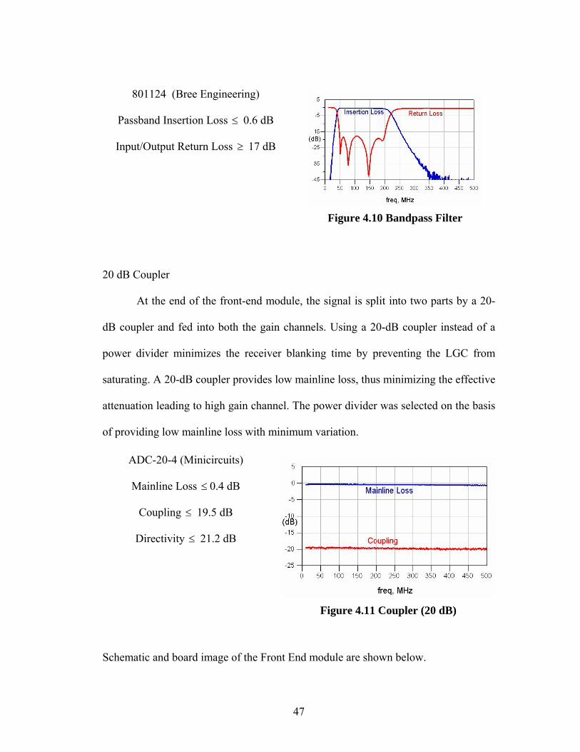
801124 (Bree Engineering)
Passband Insertion Loss ≤ 0.6 dB
Input/Output Return Loss ≥ 17 dB
Figure 4.10 Bandpass Filter
20 dB Coupler
At the end of the front-end module, the signal is split into two parts by a 20-
dB coupler and fed into both the gain channels. Using a 20-dB coupler instead of a
power divider minimizes the receiver blanking time by preventing the LGC from
saturating. A 20-dB coupler provides low mainline loss, thus minimizing the effective
attenuation leading to high gain channel. The power divider was selected on the basis
of providing low mainline loss with minimum variation.
ADC-20-4 (Minicircuits)
Mainline Loss 0.4 dB ≤
Coupling 19.5 dB ≤
Directivity 21.2 dB ≤
Figure 4.11 Coupler (20 dB)
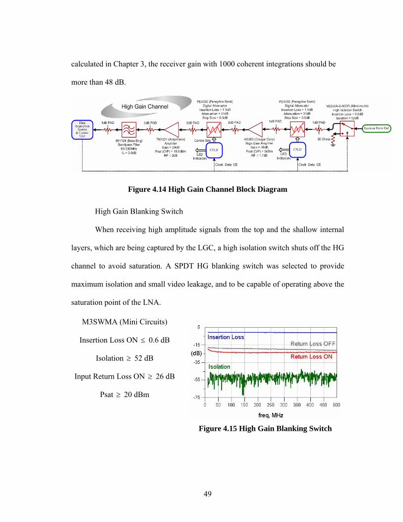
Schematic and board image of the Front End module are shown below.
47
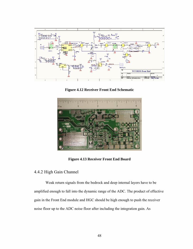
Figure 4.12 Receiver Front End Schematic
Figure 4.13 Receiver Front End Board
4.4.2 High Gain Channel
Weak return signals from the bedrock and deep internal layers have to be
amplified enough to fall into the dynamic range of the ADC. The product of effective
gain in the Front End module and HGC should be high enough to push the receiver
noise floor up to the ADC noise floor after including the integration gain. As
48
calculated in Chapter 3, the receiver gain with 1000 coherent integrations should be
more than 48 dB.
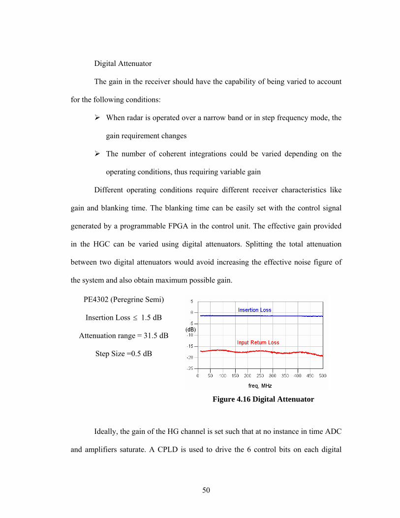
Figure 4.14 High Gain Channel Block Diagram
High Gain Blanking Switch
When receiving high amplitude signals from the top and the shallow internal
layers, which are being captured by the LGC, a high isolation switch shuts off the HG
channel to avoid saturation. A SPDT HG blanking switch was selected to provide
maximum isolation and small video leakage, and to be capable of operating above the
saturation point of the LNA.
M3SWMA (Mini Circuits)
Insertion Loss ON ≤ 0.6 dB
Isolation 52 dB ≥
Input Return Loss ON 26 dB ≥
Psat 20 dBm ≥
Figure 4.15 High Gain Blanking Switch
49
Digital Attenuator
The gain in the receiver should have the capability of being varied to account
for the following conditions:
When radar is operated over a narrow band or in step frequency mode, the
gain requirement changes
The number of coherent integrations could be varied depending on the
operating conditions, thus requiring variable gain
Different operating conditions require different receiver characteristics like
gain and blanking time. The blanking time can be easily set with the control signal
generated by a programmable FPGA in the control unit. The effective gain provided
in the HGC can be varied using digital attenuators. Splitting the total attenuation
between two digital attenuators would avoid increasing the effective noise figure of
the system and also obtain maximum possible gain.
PE4302 (Peregrine Semi)
Insertion Loss ≤ 1.5 dB
Attenuation range = 31.5 dB
Step Size =0.5 dB
Figure 4.16 Digital Attenuator
Ideally, the gain of the HG channel is set such that at no instance in time ADC
and amplifiers saturate. A CPLD is used to drive the 6 control bits on each digital
50
attenuator to set the required attenuation. The CPLD transforms the serial data from
the control unit into parallel data to set the attenuation on the digital attenuator and
provide control signals for the bi-level LEDs.
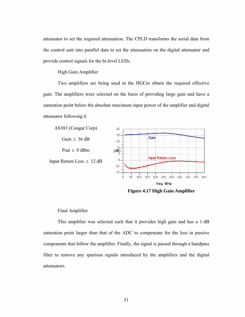
High Gain Amplifier
Two amplifiers are being used in the HGCto obtain the required effective
gain. The amplifiers were selected on the basis of providing large gain and have a
saturation point below the absolute maximum input power of the amplifier and digital
attenuator following it
AS383 (Cougar Corp)
Gain 36 dB ≥
Psat 0 dBm ≥
Input Return Loss 12 dB ≥
Figure 4.17 High Gain Amplifier
Final Amplifier
This amplifier was selected such that it provides high gain and has a 1-dB
saturation point larger than that of the ADC to compensate for the loss in passive
components that follow the amplifier. Finally, the signal is passed through a bandpass
filter to remove any spurious signals introduced by the amplifiers and the digital
attenuators.
51
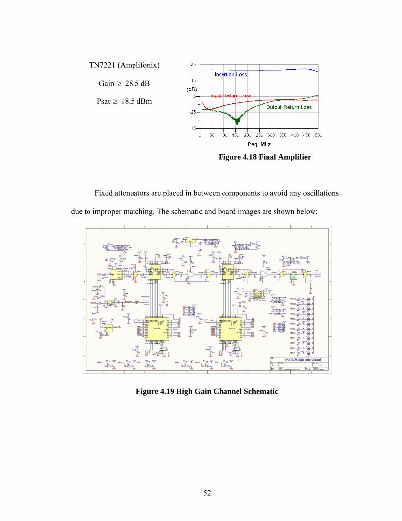
TN7221 (Amplifonix)
Gain 28.5 dB ≥
Psat 18.5 dBm ≥
Figure 4.18 Final Amplifier
Fixed attenuators are placed in between components to avoid any oscillations
due to improper matching. The schematic and board images are shown below:
Figure 4.19 High Gain Channel Schematic
52
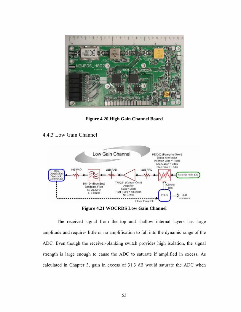
Figure 4.20 High Gain Channel Board
4.4.3 Low Gain Channel
Figure 4.21 WOCRDS Low Gain Channel
The received signal from the top and shallow internal layers has large
amplitude and requires little or no amplification to fall into the dynamic range of the
ADC. Even though the receiver-blanking switch provides high isolation, the signal
strength is large enough to cause the ADC to saturate if amplified in excess. As
calculated in Chapter 3, gain in excess of 31.3 dB would saturate the ADC when
53
receiving the reflection from the top surface. The amplification provided by the LNA
in the front-end module is almost nullified by the losses in the 20-dB coupler and
other passive components in the front-end module. Any amplification required,
should be provided in the LGC. Ability to vary the amplification in the receiver
would allow the radar to operate in different operating conditions. The LGC block
diagram, schematic and image of the board are given below.
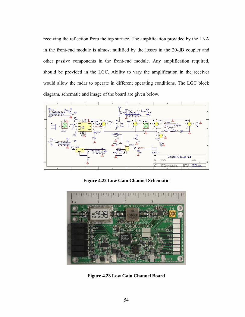
Figure 4.22 Low Gain Channel Schematic
Figure 4.23 Low Gain Channel Board
54
The design of the LGC is similar to that of the HGC except for the exclusion
of the blanking switch, high gain amplifier and a digital attenuator
4.5 Frequency Synthesizer (10 MHz to 500 MHz)
According to the Nyquist theorem, the sampling rate must be at least twice the
highest frequency component of the signal. Thus, generating or capturing a 200 MHz
analog signal would require a sampling rate higher than 400 MHz to satisfy the
Nyquist theorem. Sampling at 500 MHz would provide a guard band of 50 MHz thus
minimizing the amount of noise being coupled back into the passband due to aliasing.
The 500-MHz clock has to be phase locked to a 10-MHz stable reference clock to
simplify the synchronization requirements with other radars and communication
systems that are being operated simultaneously.
The Phase Lock Loop (PLL) chip (LMX 2326, National Semiconductors)
divides both the10-MHz reference clock and the signal from a Voltage-Controlled
Oscillator (VCO) to a small reference frequency and passes them through a phase
comparator. Depending on the phase difference between the two clocks, the phase
comparator accordingly tunes the VCO output to the required 500-MHz clock and
keeps it locked to that frequency. The PLL chip is designed by the manufacturer to
operate over a wide frequency range, so the chip needs to be programmed for it to
operate with selective frequencies. The data in the three volatile memory registers on
the PLL chip define the reference comparison frequency and functionality of the chip.
As the memory on the PLL chip is volatile, every time power is applied to the chip, it
55
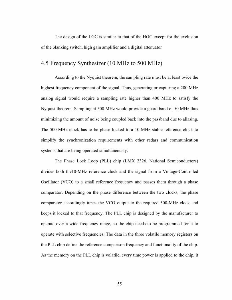
needs to be programmed. A small CPLD with non-volatile memory is being used to
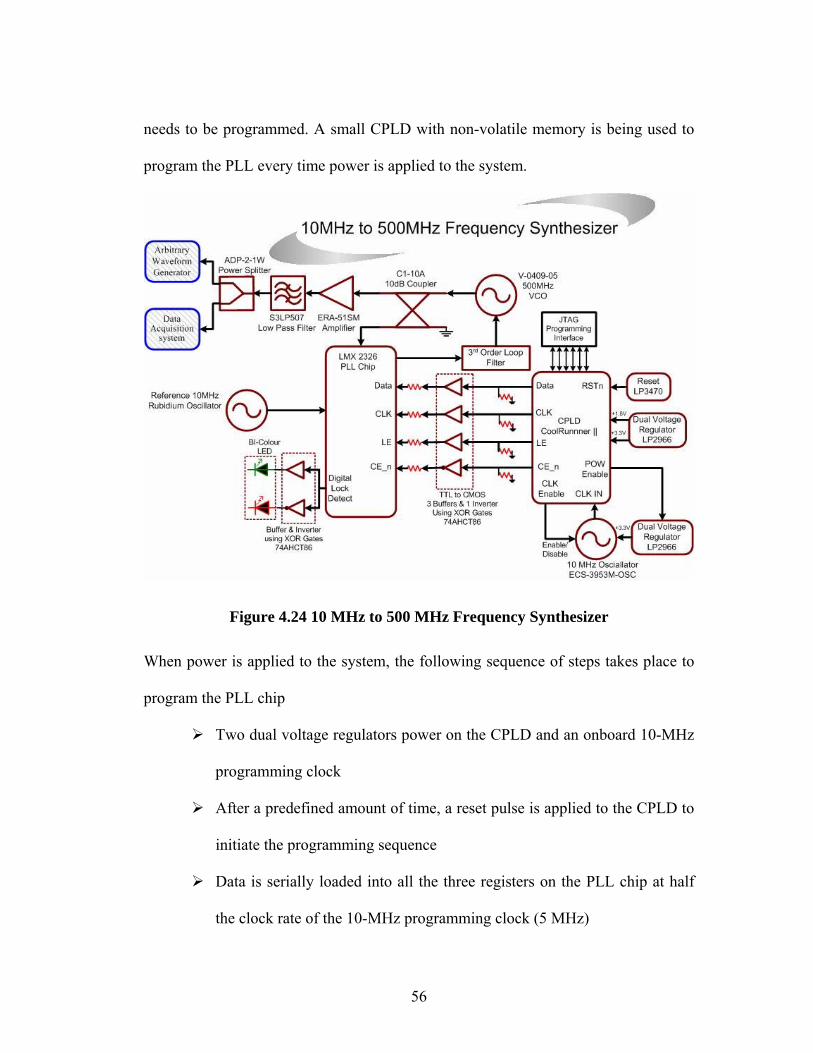
program the PLL every time power is applied to the system.
Figure 4.24 10 MHz to 500 MHz Frequency Synthesizer
When power is applied to the system, the following sequence of steps takes place to
program the PLL chip
Two dual voltage regulators power on the CPLD and an onboard 10-MHz
programming clock
After a predefined amount of time, a reset pulse is applied to the CPLD to
initiate the programming sequence
Data is serially loaded into all the three registers on the PLL chip at half
the clock rate of the 10-MHz programming clock (5 MHz)
56
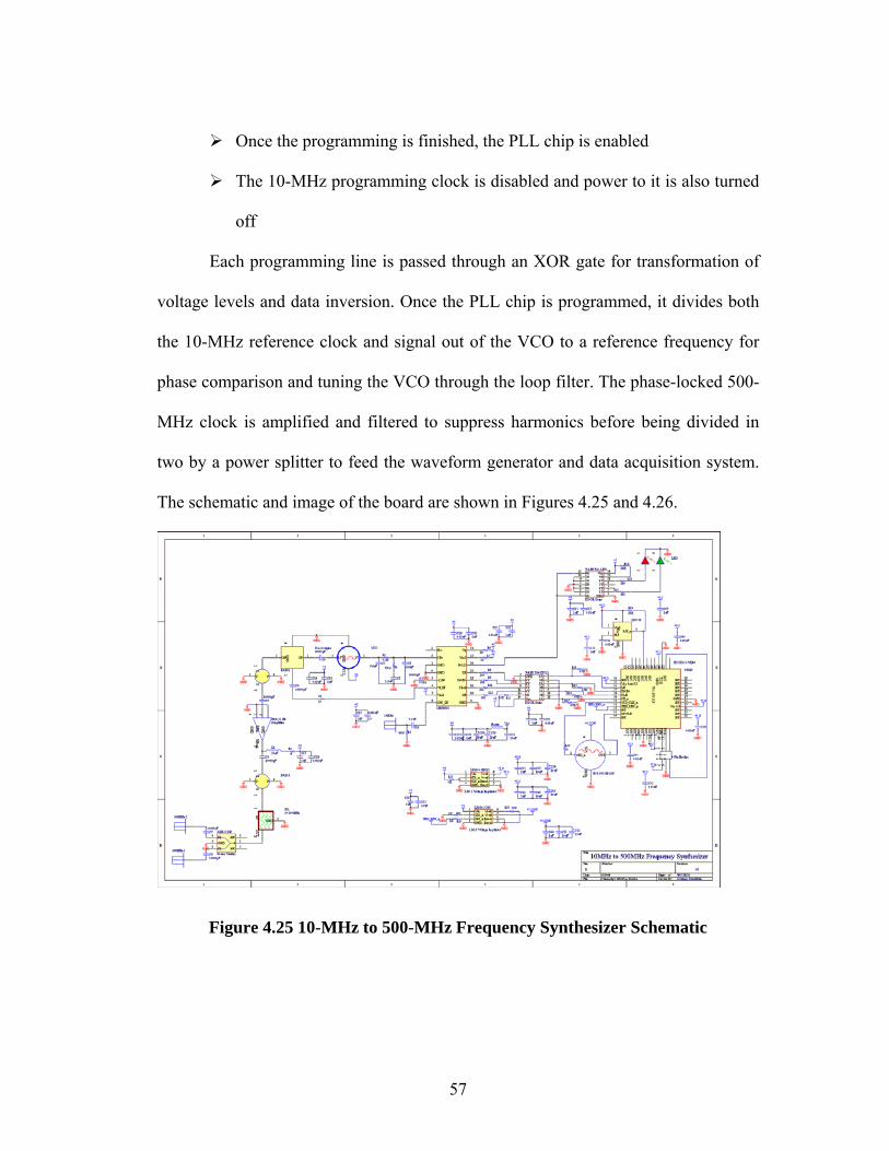
Once the programming is finished, the PLL chip is enabled
The 10-MHz programming clock is disabled and power to it is also turned
off
Each programming line is passed through an XOR gate for transformation of
voltage levels and data inversion. Once the PLL chip is programmed, it divides both
the 10-MHz reference clock and signal out of the VCO to a reference frequency for
phase comparison and tuning the VCO through the loop filter. The phase-locked 500-
MHz clock is amplified and filtered to suppress harmonics before being divided in
two by a power splitter to feed the waveform generator and data acquisition system.
The schematic and image of the board are shown in Figures 4.25 and 4.26.
Figure 4.25 10-MHz to 500-MHz Frequency Synthesizer Schematic
57
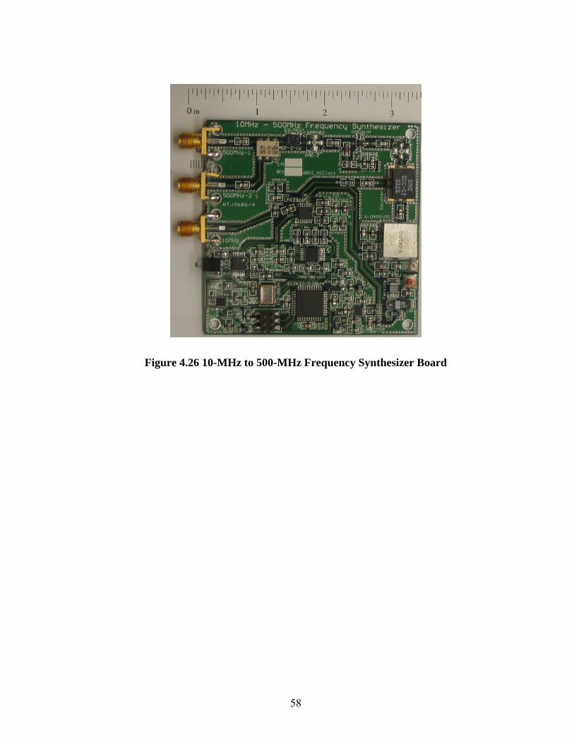
Figure 4.26 10-MHz to 500-MHz Frequency Synthesizer Board
58
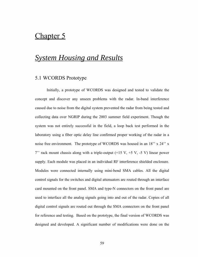
Chapter 5
System Housing and Results
5.1 WCORDS Prototype
Initially, a prototype of WCORDS was designed and tested to validate the
concept and discover any unseen problems with the radar. In-band interference
caused due to noise from the digital system prevented the radar from being tested and
collecting data over NGRIP during the 2003 summer field experiment. Though the
system was not entirely successful in the field, a loop back test performed in the
laboratory using a fiber optic delay line confirmed proper working of the radar in a
noise free environment. The prototype of WCORDS was housed in an 18’’ x 24’’ x
7’’ rack mount chassis along with a triple-output (+15 V, +5 V, -5 V) linear power
supply. Each module was placed in an individual RF interference shielded enclosure.
Modules were connected internally using mini-bend SMA cables. All the digital
control signals for the switches and digital attenuators are routed through an interface
card mounted on the front panel. SMA and type-N connectors on the front panel are
used to interface all the analog signals going into and out of the radar. Copies of all
digital control signals are routed out through the SMA connectors on the front panel
for reference and testing. Based on the prototype, the final version of WCORDS was
designed and developed. A significant number of modifications were done on the
59
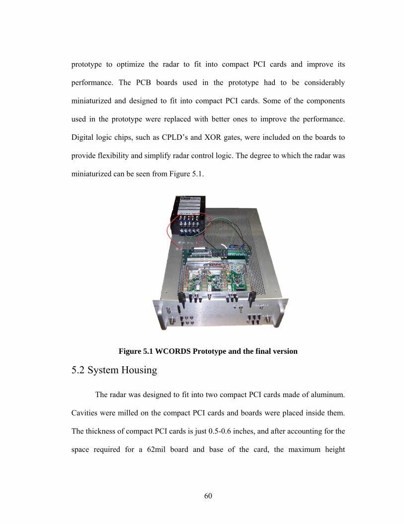
prototype to optimize the radar to fit into compact PCI cards and improve its
performance. The PCB boards used in the prototype had to be considerably
miniaturized and designed to fit into compact PCI cards. Some of the components
used in the prototype were replaced with better ones to improve the performance.
Digital logic chips, such as CPLD’s and XOR gates, were included on the boards to
provide flexibility and simplify radar control logic. The degree to which the radar was
miniaturized can be seen from Figure 5.1.
Figure 5.1 WCORDS Prototype and the final version
5.2 System Housing
The radar was designed to fit into two compact PCI cards made of aluminum.
Cavities were milled on the compact PCI cards and boards were placed inside them.
The thickness of compact PCI cards is just 0.5-0.6 inches, and after accounting for the
space required for a 62mil board and base of the card, the maximum height
60

requirement for any component was restricted to just 0.45-5 inches. While selecting
components for the radar, height limitation was also considered. The solid aluminum
base to which the modules are attached provides good grounding among modules and
acts as an excellent heat sink. Based on an approximate estimate of the size of each
board, it was decided that two compact PCI cards were required to fit all the boards.
The following issues were addressed while designing the boards
Provide the power input close to the end of the board to ease the routing
architecture on the compact PCI card
Provide good exposed ground plane on the back side of the board for
proper grounding and good heat dissipation
Appropriately place the analog inputs and outputs on the receiver boards
to provide easy and small route for the SMA cables on the compact PCI
card
Provide good power filtering on the board to reduce the amount of
switching noise coupling into analog signal
Carefully select the dimensions of the boards for optimum fit
Channels were drilled on the compact PCI cards to allow power lines and analog
SMA cables to pass through. The transmitter and the clock boards were placed on the
first card and the second card carried the receiver boards. Bulkhead SMA connectors
were used to route all the analog signal ports (Tx IN, Tx OUT, 10MHz IN, 500MHz
OUT Tx, 500MHz OUT Rx, Rx IN, HGRx OUT and LGRx OUT) going into and out
of compact PCI cards. Apart from analog signals, copies of the digital control signals
61
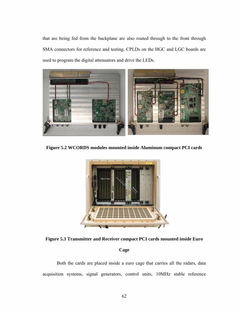
that are being fed from the backplane are also routed through to the front through
SMA connectors for reference and testing. CPLDs on the HGC and LGC boards are
used to program the digital attenuators and drive the LEDs.
Figure 5.2 WCORDS modules mounted inside Aluminum compact PCI cards
Figure 5.3 Transmitter and Receiver compact PCI cards mounted inside Euro
Cage
Both the cards are placed inside a euro cage that carries all the radars, data
acquisition systems, signal generators, control units, 10MHz stable reference
62
oscillator and power supply. Power and control signals to the radar are fed through a
backplane of the euro cage.
5.3 Results
5.3.1 Transmitter and Receiver amplitude response For each RF component used in the radar, an evaluation board was designed
and S-parameters were recorded using a network analyzer. Advance Design System
(ADS) can be used to simulate the real time performance of the radar using the S-
parameter files of each individual component. Using S-parameter files, amplitude
variation and phase nonlinearities produced by each individual component can be
removed in post processing or compensated in the transmit waveform. S-parameters
files of each component will be helpful in debugging errors during testing of the radar
and they also provide a good estimate of padding required between two components.
The simulated and measured response of each individual module will be discussed in
the following subsection.
5.3.1.1 Transmitter
The S-parameters of the transmitter were recorded with the transmitter-
blanking switch in ON and OFF positions. A close match between the measured and
simulated amplitude response of the transmitter wes obtained. Simulated and
measured amplitude response of the transmitter module is shown in Figure 5.4.
63
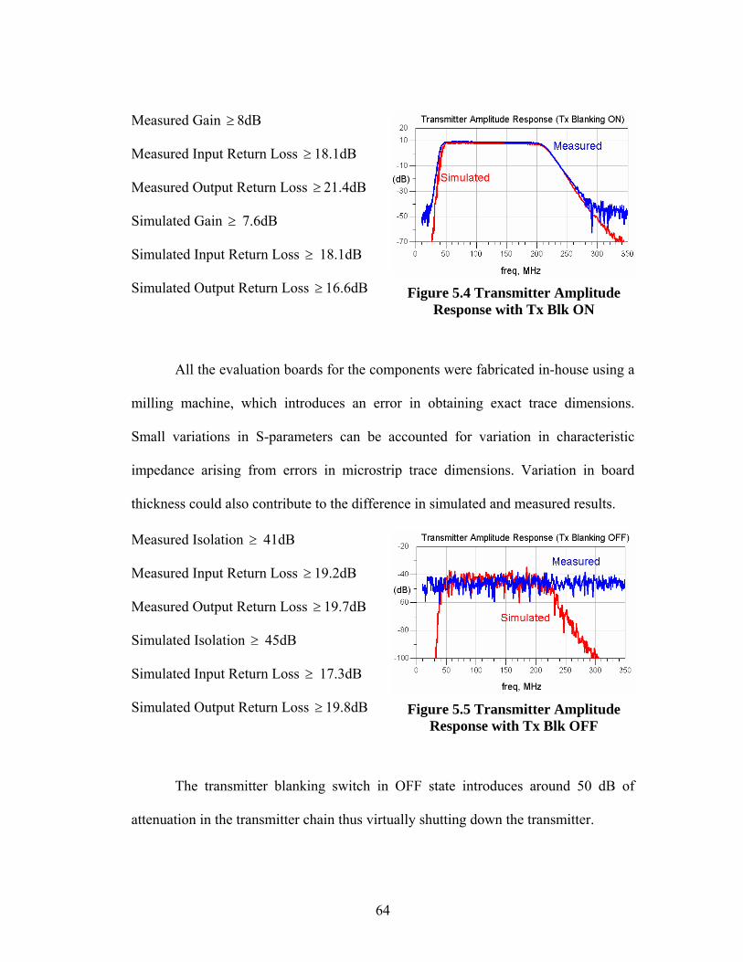
Measured Gain 8dB ≥
Measured Input Return Loss 18.1dB ≥
Measured Output Return Loss 21.4dB ≥
Simulated Gain ≥ 7.6dB
Simulated Input Return Loss 18.1dB ≥
Simulated Output Return Loss ≥ 16.6dB
Figure 5.4 Transmitter Amplitude Response with Tx Blk ON
All the evaluation boards for the components were fabricated in-house using a
milling machine, which introduces an error in obtaining exact trace dimensions.
Small variations in S-parameters can be accounted for variation in characteristic
impedance arising from errors in microstrip trace dimensions. Variation in board
thickness could also contribute to the difference in simulated and measured results.
Measured Isolation ≥ 41dB
Measured Input Return Loss 19.2dB ≥
Measured Output Return Loss 19.7dB ≥
Simulated Isolation 45dB ≥
Simulated Input Return Loss 17.3dB ≥
Simulated Output Return Loss ≥ 19.8dB
Figure 5.5 Transmitter Amplitude Response with Tx Blk OFF
The transmitter blanking switch in OFF state introduces around 50 dB of
attenuation in the transmitter chain thus virtually shutting down the transmitter.
64
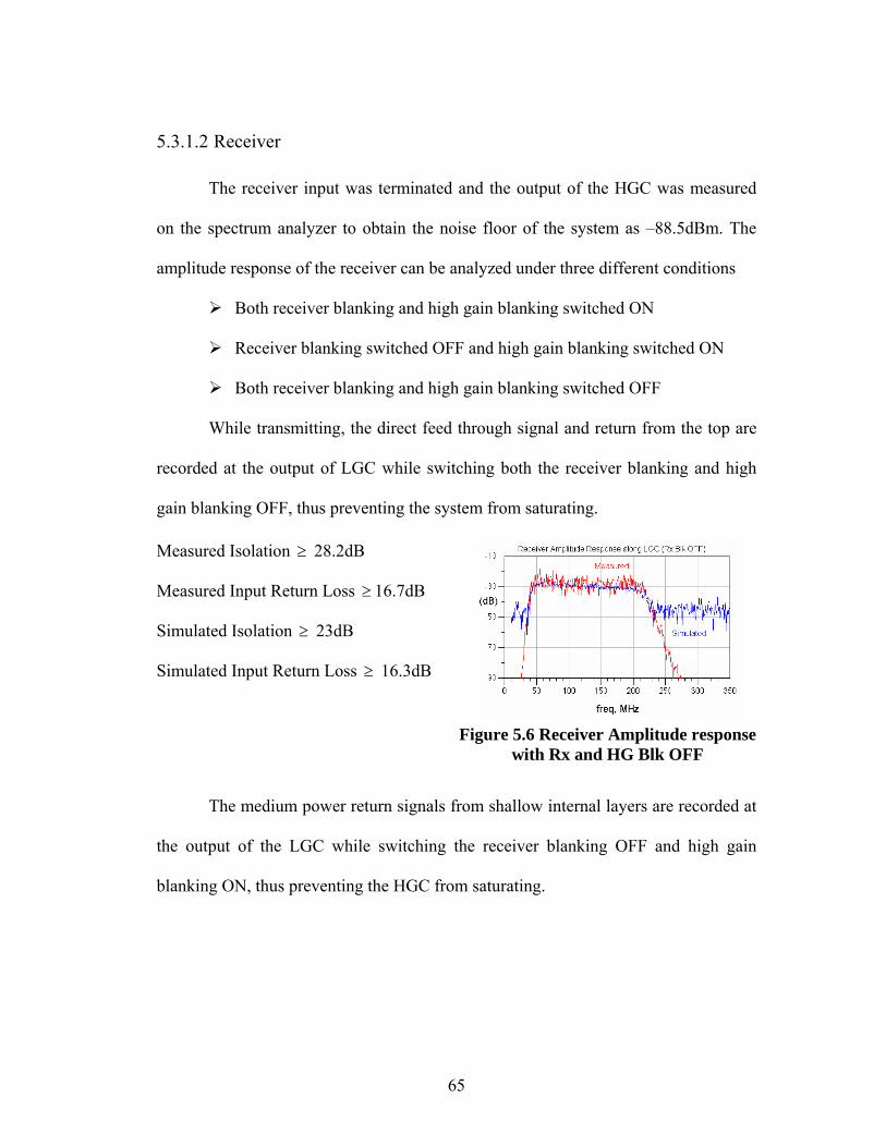
5.3.1.2 Receiver
The receiver input was terminated and the output of the HGC was measured
on the spectrum analyzer to obtain the noise floor of the system as –88.5dBm. The
amplitude response of the receiver can be analyzed under three different conditions
Both receiver blanking and high gain blanking switched ON
Receiver blanking switched OFF and high gain blanking switched ON
Both receiver blanking and high gain blanking switched OFF
While transmitting, the direct feed through signal and return from the top are
recorded at the output of LGC while switching both the receiver blanking and high
gain blanking OFF, thus preventing the system from saturating.
Measured Isolation ≥ 28.2dB
Measured Input Return Loss 16.7dB ≥
Simulated Isolation 23dB ≥
Simulated Input Return Loss 16.3dB ≥
Figure 5.6 Receiver Amplitude response
with Rx and HG Blk OFF
The medium power return signals from shallow internal layers are recorded at
the output of the LGC while switching the receiver blanking OFF and high gain
blanking ON, thus preventing the HGC from saturating.
65
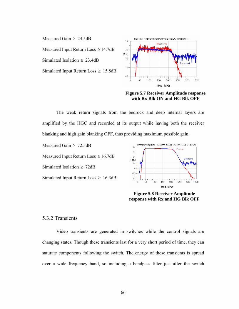
Measured Gain 24.5dB ≥
Measured Input Return Loss 14.7dB ≥
Simulated Isolation 23.4dB ≥
Simulated Input Return Loss 15.8dB ≥
Figure 5.7 Receiver Amplitude response with Rx Blk ON and HG Blk OFF
The weak return signals from the bedrock and deep internal layers are
amplified by the HGC and recorded at its output while having both the receiver
blanking and high gain blanking OFF, thus providing maximum possible gain.
Measured Gain 72.5dB ≥
Measured Input Return Loss 16.7dB ≥
Simulated Isolation 72dB ≥
Simulated Input Return Loss 16.3dB ≥
Figure 5.8 Receiver Amplitude
response with Rx and HG Blk OFF
5.3.2 Transients
Video transients are generated in switches while the control signals are
changing states. Though these transients last for a very short period of time, they can
saturate components following the switch. The energy of these transients is spread
over a wide frequency band, so including a bandpass filter just after the switch
66
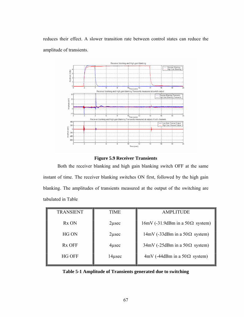
reduces their effect. A slower transition rate between control states can reduce the
amplitude of transients.
Figure 5.9 Receiver Transients
Both the receiver blanking and high gain blanking switch OFF at the same
instant of time. The receiver blanking switches ON first, followed by the high gain
blanking. The amplitudes of transients measured at the output of the switching are
tabulated in Table
TRANSIENT TIME AMPLITUDE
Rx ON 2µsec 16mV (-31.9dBm in a 50 system) Ω
HG ON 2µsec 14mV (-33dBm in a 50 system) Ω
Rx OFF 4µsec 34mV (-25dBm in a 50 system) Ω
HG OFF 14µsec 4mV (-44dBm in a 50 system) Ω
Table 5-1 Amplitude of Transients generated due to switching
67

None of the transients is big enough to saturate amplifiers that immediately
follow the switches. But, the transient noise generated when the receiver blanking
switches OFF gets amplified along the HGC to saturate the A/D in the data
acquisition system. This is caused because the high gain blanking switch takes more
time to turn OFF than the receiver blanking switch. This problem can be easily
resolved by switching OFF the high gain blanking a few clock cycles ahead of the
receiver blanking.
5.3.3 Radar Pulse Compression
A loopback test was performed on the WCORDS to analyze the radar
performance and correct the amplitude and phase nonlinearities introduced by radar.
The AWG was programmed to generate a 50-MHz to 200-MHz linear chirp over a 1-
µsec period. The chirp was first passed through the transmitter module and then
through the LCF power amplifier to be amplified to a peak power of 50W. The output
of the power amplifier was connected to high power fixed attenuators to decrease the
signal amplitude by 40dB. The signal is further attenuated by 70dB before feeding
into the receiver. The signal at the output of both the gain channels is digitized and
recorded on an oscilloscope at 2Gsps. Transmit chirp at the output of the AWG and
receive chirp at the output of HGC are shown in Figure 5.10 and Figure 5.11. The
output of LGC looks pretty same as the HGC output but at lower amplitude, so it is
not being included.
68
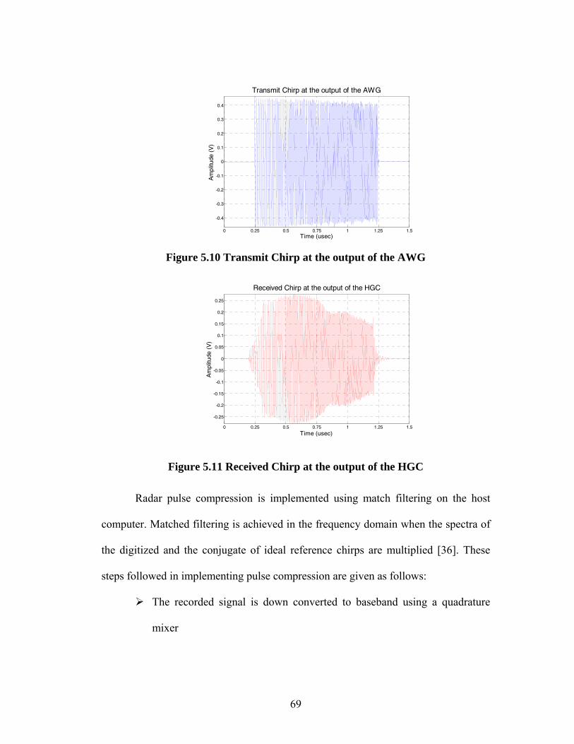
0 0.25 0.5 0.75 1 1.25 1.5
-0.4
-0.3
-0.2
-0.1
0
0.1
0.2
0.3
0.4
Time (usec)
Am
plitu
de (
V)
Transmit Chirp at the output of the AWG
Figure 5.10 Transmit Chirp at the output of the AWG
0 0.25 0.5 0.75 1 1.25 1.5
-0.25
-0.2
-0.15
-0.1
-0.05
0
0.05
0.1
0.15
0.2
0.25
Time (usec)
Am
plitu
de (
V)
Received Chirp at the output of the HGC
Figure 5.11 Received Chirp at the output of the HGC
Radar pulse compression is implemented using match filtering on the host
computer. Matched filtering is achieved in the frequency domain when the spectra of
the digitized and the conjugate of ideal reference chirps are multiplied [36]. These
steps followed in implementing pulse compression are given as follows:
The recorded signal is down converted to baseband using a quadrature
mixer
69
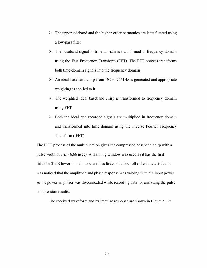
The upper sideband and the higher-order harmonics are later filtered using
a low-pass filter
The baseband signal in time domain is transformed to frequency domain
using the Fast Frequency Transform (FFT). The FFT process transforms
both time-domain signals into the frequency domain
An ideal baseband chirp from DC to 75MHz is generated and appropriate
weighting is applied to it
The weighted ideal baseband chirp is transformed to frequency domain
using FFT
Both the ideal and recorded signals are multiplied in frequency domain
and transformed into time domain using the Inverse Fourier Frequency
Transform (IFFT)
The IFFT process of the multiplication gives the compressed baseband chirp with a
pulse width of 1/B (6.66 nsec). A Hanning window was used as it has the first
sidelobe 31dB lower to main lobe and has faster sidelobe roll off characteristics. It
was noticed that the amplitude and phase response was varying with the input power,
so the power amplifier was disconnected while recording data for analyzing the pulse
compression results.
The received waveform and its impulse response are shown in Figure 5.12:
70
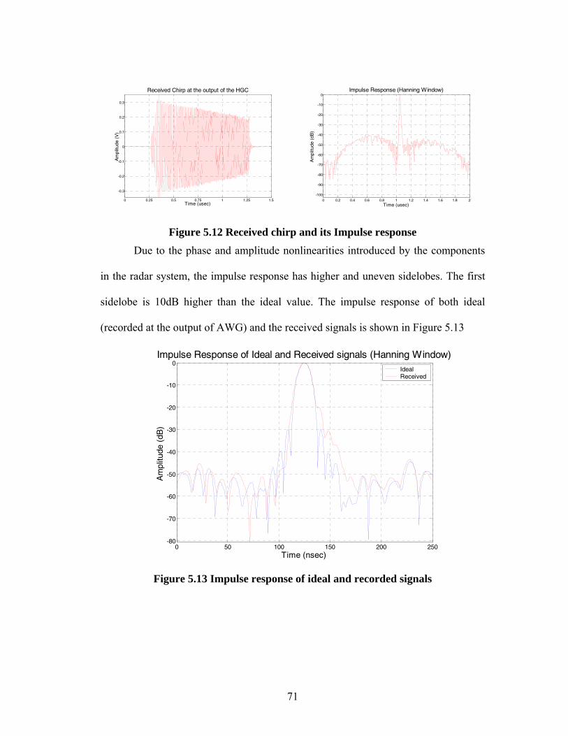
0 0.25 0.5 0.75 1 1.25 1.5
-0.3
-0.2
-0.1
0
0.1
0.2
0.3
Time (usec)
Am
plitu
de (
V)
Received Chirp at the output of the HGC
0 0.2 0.4 0.6 0.8 1 1.2 1.4 1.6 1.8 2
-100
-90
-80
-70
-60
-50
-40
-30
-20
-10
0
Time (usec)
Am
plitu
de (
dB)
Impulse Response (Hanning Window)
Figure 5.12 Received chirp and its Impulse response
Due to the phase and amplitude nonlinearities introduced by the components
in the radar system, the impulse response has higher and uneven sidelobes. The first
sidelobe is 10dB higher than the ideal value. The impulse response of both ideal
(recorded at the output of AWG) and the received signals is shown in Figure 5.13
0 50 100 150 200 250-80
-70
-60
-50
-40
-30
-20
-10
0
Time (nsec)
Am
plitu
de (
dB)
Impulse Response of Ideal and Received signals (Hanning Window)IdealReceived
Figure 5.13 Impulse response of ideal and recorded signals
71
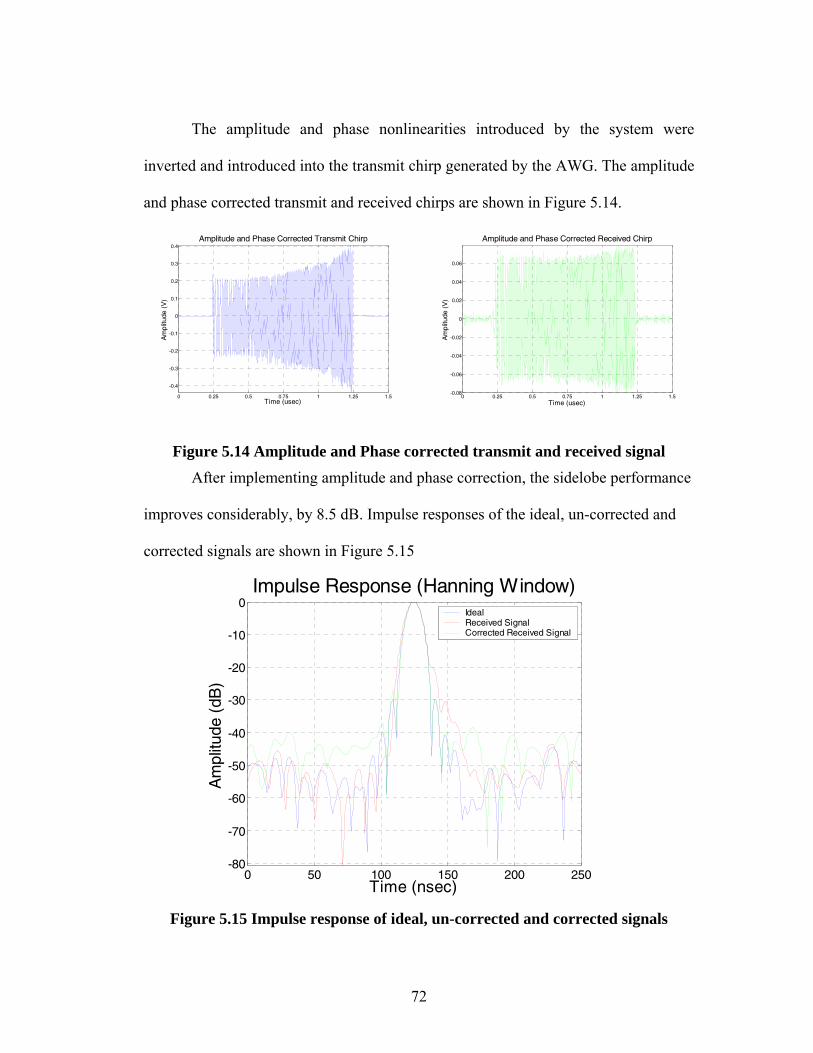
The amplitude and phase nonlinearities introduced by the system were
inverted and introduced into the transmit chirp generated by the AWG. The amplitude
and phase corrected transmit and received chirps are shown in Figure 5.14.
0 0.25 0.5 0.75 1 1.25 1.5
-0.4
-0.3
-0.2
-0.1
0
0.1
0.2
0.3
0.4
Time (usec)
Am
plitu
de (
V)
Amplitude and Phase Corrected Transmit Chirp
0 0.25 0.5 0.75 1 1.25 1.5-0.08
-0.06
-0.04
-0.02
0
0.02
0.04
0.06
Time (usec)
Am
plitu
de (
V)
Amplitude and Phase Corrected Received Chirp
Figure 5.14 Amplitude and Phase corrected transmit and received signal
After implementing amplitude and phase correction, the sidelobe performance
improves considerably, by 8.5 dB. Impulse responses of the ideal, un-corrected and
corrected signals are shown in Figure 5.15
0 50 100 150 200 250-80
-70
-60
-50
-40
-30
-20
-10
0
Time (nsec)
Am
plitu
de (
dB)
Impulse Response (Hanning Window)IdealReceived SignalCorrected Received Signal
Figure 5.15 Impulse response of ideal, un-corrected and corrected signals
72
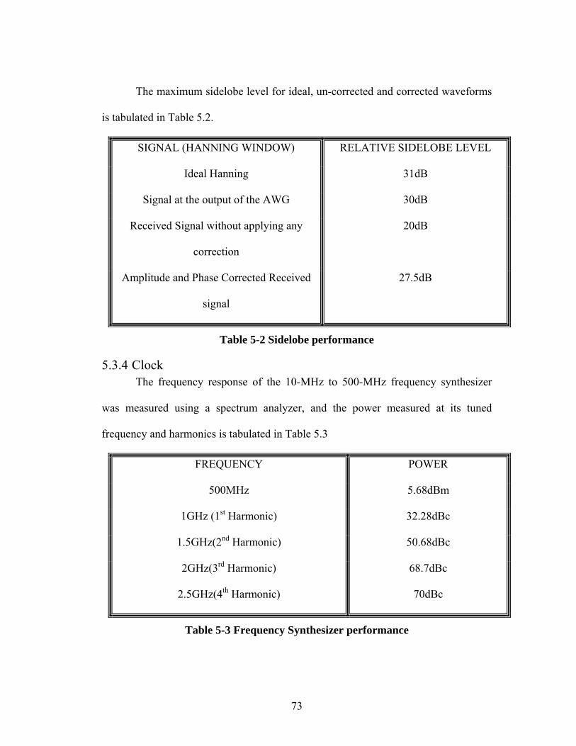
The maximum sidelobe level for ideal, un-corrected and corrected waveforms
is tabulated in Table 5.2.
SIGNAL (HANNING WINDOW) RELATIVE SIDELOBE LEVEL
Ideal Hanning 31dB
Signal at the output of the AWG 30dB
Received Signal without applying any
correction
20dB
Amplitude and Phase Corrected Received
signal
27.5dB
Table 5-2 Sidelobe performance
5.3.4 Clock The frequency response of the 10-MHz to 500-MHz frequency synthesizer
was measured using a spectrum analyzer, and the power measured at its tuned
frequency and harmonics is tabulated in Table 5.3
FREQUENCY POWER
500MHz 5.68dBm
1GHz (1st Harmonic) 32.28dBc
1.5GHz(2nd Harmonic) 50.68dBc
2GHz(3rd Harmonic) 68.7dBc
2.5GHz(4th Harmonic) 70dBc
Table 5-3 Frequency Synthesizer performance
73
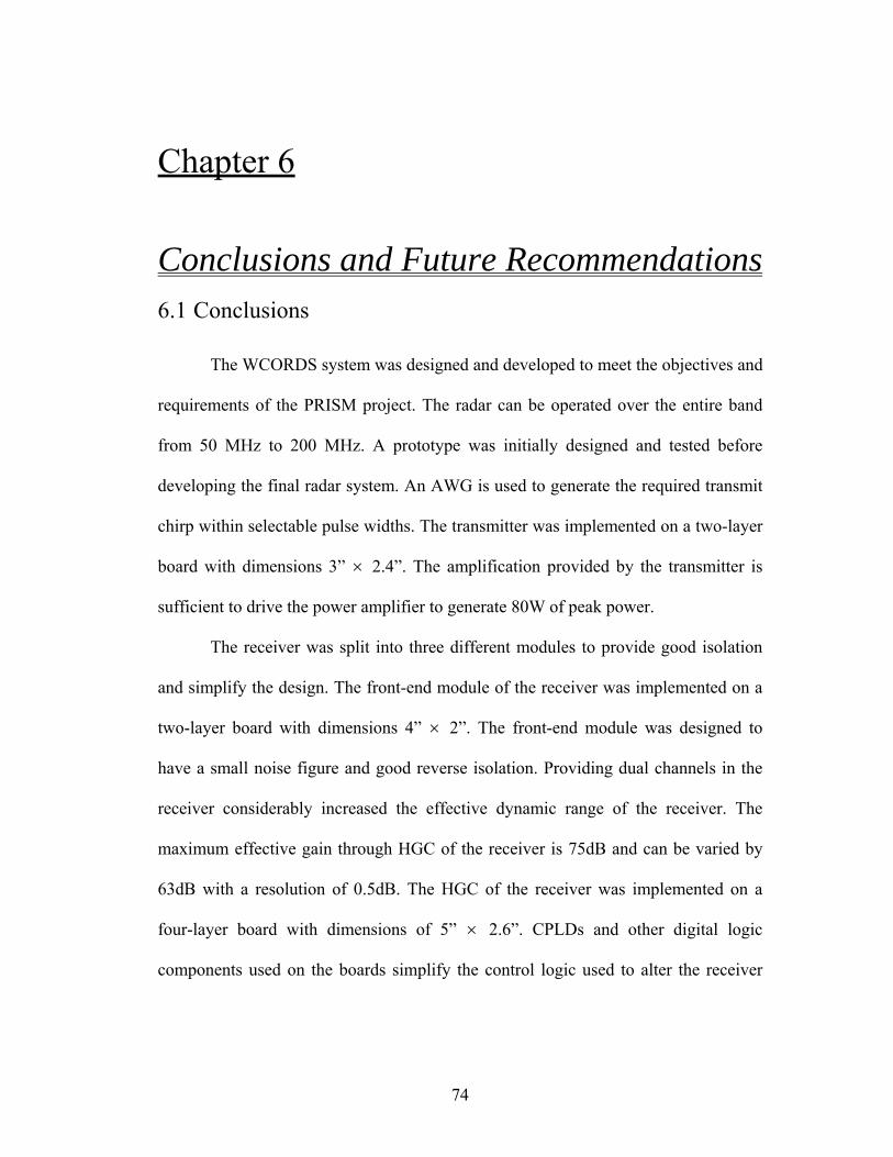
Chapter 6
Conclusions and Future Recommendations 6.1 Conclusions
The WCORDS system was designed and developed to meet the objectives and
requirements of the PRISM project. The radar can be operated over the entire band
from 50 MHz to 200 MHz. A prototype was initially designed and tested before
developing the final radar system. An AWG is used to generate the required transmit
chirp within selectable pulse widths. The transmitter was implemented on a two-layer
board with dimensions 3” × 2.4”. The amplification provided by the transmitter is
sufficient to drive the power amplifier to generate 80W of peak power.
The receiver was split into three different modules to provide good isolation
and simplify the design. The front-end module of the receiver was implemented on a
two-layer board with dimensions 4” × 2”. The front-end module was designed to
have a small noise figure and good reverse isolation. Providing dual channels in the
receiver considerably increased the effective dynamic range of the receiver. The
maximum effective gain through HGC of the receiver is 75dB and can be varied by
63dB with a resolution of 0.5dB. The HGC of the receiver was implemented on a
four-layer board with dimensions of 5” × 2.6”. CPLDs and other digital logic
components used on the boards simplify the control logic used to alter the receiver
74
parameters. The LGC was implemented on a four-layer board with dimensions of
3.9” × 1.9”.
The 10Mhz to 500MHz frequency synthesizer provides a clean and stable
clock to the waveform generator and the data acquisition system. The clock system
was implemented on a 3” × 3” four-layer board. Considerable improvement in the
sidelobe levels was noticed after including the phase and amplitude nonlinearities in
the transmit pulse. Summarized below are some important characteristics of the radar
Ability to detect ice thickness up to 4km
Map deep internal layers with a resolution of 56cm
Obtain important information about ice sheet basal properties and
scattering characteristics over a wide frequency range
Small and compact
The WCORDS system will be mounted inside an automated rover and tested
in Greenland during the 2004 field season.
6.2 Future Recommendations
Power amplifiers for the land based (50W) and airborne (200W) operation are
mounted inside rack mount chassis, which makes the entire system big, heavy and
unwieldy. Highly efficient and linear class E power amplifiers can be designed to
output 200W and fit on a single compact PCI card. Another possible solution that can
be adopted is to divide the transmit signal into multiple channels and amplify the
signal in each channel using small and readily available power amplifiers. The output
75
of each power amplifier can be fed into single or multiple elements of an antenna
array.
Better resolution can be obtained if the radar is operated over a wider band.
With the advent of recently developed wideband antennas and with few modifications
to the radar and the data acquisition system, the radar can be operated up to 400 MHz.
And as calculated in chapter 3, the loss through ice is pretty much constant over the
frequency band 50 MHz to 400 MHz.
As the radar hasn’t been tested in the field, at this point in time, not many
improvements regarding system operation can be suggested.
76

References
[1] Gogineni, S., PRISM proposal report (unpublished), 2000-2002
[2] James, G.T. and Vijay Narayanan. “The Probability of Sea level rise,” Library
of U.S. Global Change Research Information Center, September 1995.
[3] Hollin, J.T. and R.G.Barry, “Empirical and Theoretical Evidence Concerning
the Response of the Earth’s Ice and Snow Cover to a Global Temperature
Increase,” Environmental International vol. 2, pp 437-44, 1979.
[4] Goodwin, I., and C.Bentley, “ISMASS,” U.S. Geological Survey ISMASS 2255
N. Gemini Dr., Flagstaff, AZ (www.antcrc.utas.edu.au/scar/ismass.html).
[5] Chuah, T.S., “Design and Development of a Coherent Radar Depth Sounder for
Measurement of Greenland Ice Sheet Thickness,” RSL Technical. Report
10470-5, January 1997.
[6] Saikiran, P.V.Namburi, “Design and Development of an Advanced Coherent
Radar Depth Sounder,” RSL Technical Report, 2003.
[7] Gogineni, S., T.S. Chuah, C. Allen, K. Jezek, and R.K. Moore, “An improved
coherent radar dept sounder,” Journal of Glaciology, vol. 44, no. 148, pp. 659-
669, 1998.
[8] Waite, A.H. and S.J Schmidt, “Gross errors in height indication from pulsed
radar altimeter operating over thick ice or snow,” Institute of Radio Engineers
International Conventional Record, no 5, pp. 38-53.
77
[9] Robin, G. de Q., “Polar ice sheets: a review,” Polar Rec, vol. 16, no. 100, pp. 5-
22.
[10] Drewry, D.J., “Comparison of electromagnetic and seismic-fravity ice thickness
measurements in East Antarctica,” J.Glaciol, vol. 15, no. 73, pp. 137-150, 1975.
[11] Raju, G, “Coherent Antarctic Radar Depth Sounder (CARDS): Design,
Development and Results,” PhD Dissertation, University of Kansas, School of
Engineering, 1989.
[12] Sinsheimer, R.L. “Altitude determination,” in Hall, J.S., ed., Radar aids to
navigation, New York, McGraw-Hill, pp. 131-142, 1947.
[13] Walfol, M.E.R., “Radio echo sounding through ice shelf,” Nature, vol. 204, no.
4956, pp. 317-319, 1964.
[14] Fedorov, B.A., “Primeneniye aktivnoy radiolokatsii dly izucheniya
antarkticheskikh lednikov [Radar sounding of Antarctica ice],” Inf. Byull. Sov.
Antarkt. Eksped, vol. 62, pp. 19-24, 1967.
[15] Rinker, J.N., and S.J. Mock, “Radar ice thickness profiles – northwest
Greenland,” CRREL Spec Rep 103, 1967.
[16] Evans, S., “Progress report on radio echo sounding,” Polar Rec., vol. 13, no. 85,
pp. 413-420, 1967.
[17] Evans, S., ed., “Review of radio echo system performance in Gudmandsen,
P.E.,” Proceedings of the International Meeting on Radioglaciology, Lyngby,
Denmark, pp. 100-102, 1970.
78
[18] Evans, S., and B.M.E. Smith, “A radio echo equipment for depth sounding in
polar ice sheets,” Journal of Physics. E, Ser.2, vol. 2, pp.131-136, 1969.
[19] Jazek, K., “Radar measurement of borehole geometry on the Greenland and
Antarctica ice sheets,” Geophysics, vol. 50, no. 2, pp. 242-251, 1985.
[20] Bjornsson, H., R.L. Ferrari, K.J. Miller and G. Owen, “A 1976 radio echo
sounding expedition to the Vatnajokull ice cap, Iceland,” Polar Rec, vol. 18, no.
15, pp. 375-377, 1977.
[21] Sverrisson, M., E. Johannesson and H. Bjornsson, “Radio-echo equipment for
depth sounding of temperate glaciers,” Journal of Glaciol, vol. 25, no. 93, pp.
477-486, 1980.
[22] Allen, C., “Parameters of Time-Domain Radio Depth Sounder Systems reported
in the literature,” University of Kansas, unpublished, 1996.
[23] Fujita, S.; Matsuoka, T.; Ishida, T.; Matsuoka, K.; and Mae, S., “A summary of
complex dielectric permittivity of ice in the megahertz range and its applications
for radar sounding of polar ice sheets,” International Symposium on Physics of
Ice Core Records, Shikotsukohan, Japan, Sept. 14-17, pp. 185-212, 1998.
[24] Demarest, K.R., “Engineering Electromagnetics,” Prentice Hall, Inc., New
Jersey, ISBN: 0023285214, 1998.
[25] Matzler, C. and U.J. Wegmuller, “Dielectric properties of freshwater ice at
microwave frequencies,” Applied Physics, vol. 20, no. 12, pp. 1623-1630, 1987.
79
[26] Matsuoka, T., S. Fujita, and S. Mae, “Effect of temperature on dielectric
properties of ice in the range 5-39 GHz,” Journal of Applied Physics, vol 80, no
10, pp. 5884-5890, Nov. 15, 1996.
[27] Ulaby, F.T., R.K. Moore, and A.K Fung, Microwave Remote Sensing vol. III,
Artech House, Norwood, MA, 1986.
[28] Robin, G. de Q. S. Evans and J.T Bailey, “Interpretation of radio echo sounding
in polar ice sheets,” Philosophical Transactions of Royal Society, London, vol.
A256, no. 1166, pp. 437-505, 1969.
[29] Tiuri, M.E., A.H. Sihvol.a, E.G Nyfors and M.T. Hallikainen, “The complex
dielectric constant of snow at microwave frequencies,” IEEE Journal of Oceanic
Engineering, oe-9, pp. 377-382, 1984.
[30] Glen, J.W. and J.G. Paren, “The electrical properties of snow and ice,” Journal
of Glaciol, vol.15, no. 73, pp. 15-38, 1975.
[31] Paden, J., C.T. Allen, S.P. Gogineni, D. Dahl-Jensen, L.B. Larsen, and K.C.
Jezek, “Wideband Measurements of Basal Scattering and Ice Sheet
Attenuation,” (submitted), TGARS 2003-2004.
[32] Wolff, E.W., “Nitrate in polar ice,” Journal of Geophysics Res. 100, pp. 16249-
16264, 1995.
[33] Ewen B.M. Smith and S. Evans, “Radio echo sounding: Absorbtion and
Scattering by Water inclusion and Ice Lenses,” Journal of Glaciol, vol. 11, no
61, pp. 133-147, 1972.
80
[34] Stratton, J.A., Electromagnetic Theory, McGraw-Hill Book Co, ASIN:
0070621500, 1941.
[35] Matzler, C. and U.J. Wegmuller, Applied Physics, vol 20, pp 1623-1630, 1987.
[36] Wehner, D.R., High-resolution radar, second ed., Artech House, Inc., Norwood,
Massachusetts, 1995
[37] Henslee, J., “Antenna Design for polar ice radars,” RSL Technical Report,
2003.
81