about+the+helm+project+ -...

Production of this 2015 edition, containing corrections and minor revisions of the 2008 edition, was funded by the sigma Network.

About the HELM Project HELM (Helping Engineers Learn Mathematics) materials were the outcome of a three-‐year curriculum development project undertaken by a consortium of five English universities led by Loughborough University, funded by the Higher Education Funding Council for England under the Fund for the Development of Teaching and Learning for the period October 2002 – September 2005, with additional transferability funding October 2005 – September 2006. HELM aims to enhance the mathematical education of engineering undergraduates through flexible learning resources, mainly these Workbooks. HELM learning resources were produced primarily by teams of writers at six universities: Hull, Loughborough, Manchester, Newcastle, Reading, Sunderland. HELM gratefully acknowledges the valuable support of colleagues at the following universities and colleges involved in the critical reading, trialling, enhancement and revision of the learning materials: Aston, Bournemouth & Poole College, Cambridge, City, Glamorgan, Glasgow, Glasgow Caledonian, Glenrothes Institute of Applied Technology, Harper Adams, Hertfordshire, Leicester, Liverpool, London Metropolitan, Moray College, Northumbria, Nottingham, Nottingham Trent, Oxford Brookes, Plymouth, Portsmouth, Queens Belfast, Robert Gordon, Royal Forest of Dean College, Salford, Sligo Institute of Technology, Southampton, Southampton Institute, Surrey, Teesside, Ulster, University of Wales Institute Cardiff, West Kingsway College (London), West Notts College.

HELM Contacts: Post: HELM, Mathematics Education Centre, Loughborough University, Loughborough, LE11 3TU. Email: [email protected] Web: http://helm.lboro.ac.uk

HELM Workbooks List 1 Basic Algebra 26 Functions of a Complex Variable 2 Basic Functions 27 Multiple Integration 3 Equations, Inequalities & Partial Fractions 28 Differential Vector Calculus 4 Trigonometry 29 Integral Vector Calculus 5 Functions and Modelling 30 Introduction to Numerical Methods 6 Exponential and Logarithmic Functions 31 Numerical Methods of Approximation 7 Matrices 32 Numerical Initial Value Problems 8 Matrix Solution of Equations 33 Numerical Boundary Value Problems 9 Vectors 34 Modelling Motion 10 Complex Numbers 35 Sets and Probability 11 Differentiation 36 Descriptive Statistics 12 Applications of Differentiation 37 Discrete Probability Distributions 13 Integration 38 Continuous Probability Distributions 14 Applications of Integration 1 39 The Normal Distribution 15 Applications of Integration 2 40 Sampling Distributions and Estimation 16 Sequences and Series 41 Hypothesis Testing 17 Conics and Polar Coordinates 42 Goodness of Fit and Contingency Tables 18 Functions of Several Variables 43 Regression and Correlation 19 Differential Equations 44 Analysis of Variance 20 Laplace Transforms 45 Non-‐parametric Statistics 21 z-‐Transforms 46 Reliability and Quality Control 22 Eigenvalues and Eigenvectors 47 Mathematics and Physics Miscellany 23 Fourier Series 48 Engineering Case Study 24 Fourier Transforms 49 Student’s Guide 25 Partial Differential Equations 50 Tutor’s Guide

© Copyright Loughborough University, 2015

ContentsContents 4646

Quality Control Reliability and

46.1 Reliability 2

46.2 Quality Control 21

Learning

You will first learn about the importance of the concept of reliability applied to systems and products. The second Section introduces you to the very important topic of quality control in production processes. In both cases you will learn how to perform the basic calculations necessary to use each topic in practice.

outcomes

Reliability��

��46.1

IntroductionMuch of the theory of reliability was developed initially for use in the electronics industry wherecomponents often fail with little if any prior warning. In such cases the hazard function or conditionalfailure rate function is constant and any functioning component or system is taken to be ‘as new’.There are other cases where the conditional failure rate function is time dependent, often proportionalto the time that the system or component has been in use. The function may be an increasing functionof time (as with random vibrations for example) or decreasing with time (as with concrete whosestrength, up to a point, increases with time). If we can develop a lifetime model, we can use it toplan such things as maintenance and part replacement schedules, whole system replacements andreliability testing schedules.

#

"

!Prerequisites

Before starting this Section you should . . .

• be familiar with the results and concepts metin the study of probability

• understand and be able to use continuousprobability distributions'

&

$

%

Learning OutcomesOn completion you should be able to . . .

• appreciate the importance of lifetimedistributions

• complete reliability calculations for simplesystems

• state the relationship between the Weibulldistribution and the exponential distribution

2 HELM (2015):Workbook 46: Reliability and Quality Control

®

1. Reliability

Lifetime distributionsFrom an engineering point of view, the ability to predict the lifetime of a whole system or a systemcomponent is very important. Such lifetimes can be predicted using a statistical approach usingappropriate distributions. Common examples of structures whose lifetimes we need to know areairframes, bridges, oil rigs and at a simpler, less catastrophic level, system components such as cyclechains, engine timing belts and components of electronic systems such as televisions and computers.If we can develop a lifetime model, we can use it to plan such things as maintenance and partreplacement schedules, whole system replacements and reliability testing schedules.

We start by looking at the length of use of a system or component prior to failure (the age prior tofailure) and from this develop a definition of reliability. Lifetime distributions are functions of timeand may be expressed as probability density functions and so we may write

F (t) =

∫ t

0

f(t) dt

This represents the probability that the system or component fails anywhere between 0 and t.

Key Point 1

The probability that a system or component will fail only after time t may be written as

R(t) = 1− F (t)

The function R(t) is usually called the reliability function.

In practice engineers (and others!) are often interested in the so-called hazard function or conditionalfailure rate function which gives the probability that a system or component fails after it has been inuse for a given time. This function may be defined as

H(t) = lim∆t→o

(P(failure in the interval (t, t+ ∆t))/∆t

P(survival up to time t)

)=

1

R(t)lim

∆t→o

(F (t+ ∆t)− F (t)

∆t

)=

1

R(t)

d

dtF (t)

=f(t)

R(t)

HELM (2015):Section 46.1: Reliability

3

This gives the conditional failure rate function as

H(t) = lim∆t→o

∫ t+∆t

t

f(t) dt/(∆t)

R(t)

=

f(t)

R(t)

Essentially we are describing the rate of failure per unit time for (say) mechanical or electricalcomponents which have already been in service for a given time. A graph of H(t) often shows a highinitial failure rate followed by a period of relative reliability followed by a period of increasingly highfailure rates as a system or component ages. A typical graph (sometimes called a bathtub graph) isshown below.

H(t)

0 t

Early life andrandom failure Useful life and random failure

End of life andrandom failure

Figure 1

Note that ‘early life and random failure’ includes failure due to defects being present and that ‘endof life and random failure’ includes failure due to ageing.

The reliability of a system or component may be defined as the probability that the system orcomponent functions for a given time, that is, the probability that it will fail only after the giventime. Put another way, R(t) is the probability that the system or component is still functioning attime t.

The exponential distributionWe have already met the exponential distribution in the form

f(t) = λe−λt, t ≥ 0

However, one of the simplest distributions describing failure is the exponential distribution

f(t) =1

µe−t/µ, t ≥ 0

where, in this case, µ is the mean time to failure. One property of this distribution is that the hazardfunction is a constant independent of time - the ‘good as new’ syndrome mentioned above. To showthat the probability of failure is independent of age consider the following.

F (t) =

∫ t

0

1

µe−t/µ dt =

1

µ

[− µe−t/µ

]t0

= 1− e−t/µ


®

Hence the reliability (given that the total area under the curve F (t) = 1− e−t/µ is unity) is

R(t) = 1− F (t) = e−t/µ

Hence, the hazard function or conditional failure rate function H(t) is given by

H(t) =F (t)

R(t)=

1µ

e−t/µ

e−t/µ=

1

µ

which is a constant independent of time.

Another way of looking at this is to consider the probability that failure occurs in the interval (τ, τ+t)given that the system is functioning at time τ . This probability is

F (τ + t)− F (τ)

R(t)=

(1− e−(τ+t)/µ)− (1− e−τ/µ)

e−τ/µ

= 1− e−t/µ

This is just the probability that failure occurs in the interval (0, t) and implies that ageing has noeffect on failure. This is sometimes referred to as the ‘good as new syndrome.’

It is worth noting that in the modelling of many complex systems it is assumed that only randomcomponent failures are important. This enables us to assume the use of the exponential distributionsince initial failures are removed by a ‘running-in’ process and the time to ultimate failure is usuallylong.

Example 1The lifetime of a modern low-wattage electronic light bulb is known to be expo-nentially distributed with a mean of 8000 hours.

Find the proportion of bulbs that may be expected to fail before 7000 hours use.

Solution

We know that µ = 8000 and so

F (t) =

∫ t

0

1

8000e−t/8000 dt

=1

8000

[− 8000e−t/8000

]t0

= 1− e−t/8000

Hence F (7000) = 1 − e−7000/8000 = 1 − e−0.675 = 0.4908 and we expect that about 49% of thebulbs will fail before 7000 hours of use.


5

TaskA particular electronic device will only function correctly if two essential compo-nents both function correctly. The lifetime of the first component is known to beexponentially distributed with a mean of 6000 hours and the lifetime of the secondcomponent is known to be exponentially distributed with a mean of 7000 hours.Find the proportion of devices that may be expected to fail before 8000 hours use.State clearly any assumptions you make.

Your solution

AnswerThe assumption made is that the components operate independently.

For the first component F (t) = 1−e−t/6000 so that F (8000) = 1−e−8000/6000 = 1−e−4/3 = 0.7364

For the second component F (t) = 1− e−t/7000 so that F (8000) = 1− e−8000/7000 = 0.6811

The probability that the device will continue to function after 8000 hours use is given by an expressionof the form P(A ∪B) = P(A) + P(B)− P(A ∩B)

Hence the probability that the device will continue to function after 8000 hour use is

0.7364 + 0.6811− 0.7364× 0.6811 = 0.916

and we expect just under 92% of the devices to fail before 8000 hours use.

An alternative answer may be obtained more directly by using the reliability function R(t):

The assumption made is that the components operate independently.

For the first component R(t) = e−t/6000 so that R(8000) = e−8000/6000 = e−4/3 = 0.2636

For the second component R(t) = e−t/7000 so that R(8000) = e−8000/7000 = 0.3189

The probability that the device will continue to function after 8000 hour use is given by

0.2636× 0.3189 = 0.0841

Hence the probability that the device will fail before 8000 hours use is 1− 0.0841 = 0.916

and we expect just under 92% of the devices to fail before 8000 hours use.


®

2. System reliabilityIt is reasonable to ask whether, in designing a system, an engineer should design a system usingcomponents in series or in parallel. The engineer may not have a choice of course! We may representa system consisting of n components say C1, C2 . . . , Cn with reliabilities (these are just probabilityvalues) R1, R2 . . . , Rn respectively as series and parallel systems as shown below.

C1

C1 C2 Cn

C2

Cn

Series Design Parallel DesignFigure 2

With a series design, the system will fail if any component fails. With a parallel design, the systemwill work as long as any component works.

Assuming that the components are independent, we can express the reliability of the series design as

RSeries = R1 ×R2 × · · · ×Rn

simply by multiplying the probabilities.

Since each reliability value is less than one, we may conclude that a series design is less reliable thanits least reliable component.

Similarly (although by no means as clearly!), we can express the reliability of the parallel design as

RParallel = 1− (1−R1)(1−R2) . . . (1−Rn)

The derivation of this result is illustrated in Example 3 below for the case n = 3 . In this case,the algebra involved in fairly straightforward. We can conclude that the parallel design is at least asreliable as the most reliable component.

Engineers will sometimes include ‘redundant’components in parallel to improve reliability. The sparewheel of a car is a well known example.


7

Example 2Series design

Consider the three components C1, C2 and C3 with reliabilities R1, R2 and R3

connected in series as shown below

C1 C2 C!

Find the reliability of the system where R1 = 0.2, R2 = 0.3 and R3 = 0.4.

Solution

Since the components are assumed to act independently, we may clearly write

RSeries = R1 ×R2 ×R3

Taking R1 = 0.2, R2 = 0.3 and R3 = 0.4 we obtain the value RSeries = 0.2× 0.3× 0.4 = 0.024

Example 3Parallel design

Consider the three components C1, C2 and C3 with reliabilities R1, R2 and R3

connected in parallel as shown below

C1

C2

C!

Find the reliability of the system where R1 = 0.2, R2 = 0.3 and R3 = 0.4.

Solution

Observing that Fi = 1−Ri, where Fi represents the failure of the ith component and Ri representsthe reliability of the ith component we may write

FSystem = F1F2F3 → RSystem = 1− F1F2F3 = 1− (1−R1)(1−R2)(1−R3)

Again taking R1 = 0.2, R2 = 0.3 and R3 = 0.4 we obtain

FSystem = 1− (1− 0.2)(1− 0.3)(1− 0.4) = 1− 0.336 = 0.664


®

Hence series system reliability is less than any of the component reliabilities and parallel systemreliability is greater than any of the component reliabilities.

TaskConsider the two components C1 and C2 with reliabilities R1 and R2 connectedin series and in parallel as shown below. Assume that R1 = 0.3 and R2 = 0.4.

C1 C2

C1

C2

Series configuration Parallel configuration

Let RSeries be the reliability of the series configuration and RParallel be the reliabilityof the parallel configuration

(a) Why would you expect that RSeries < 0.3 and RParallel > 0.4?

(b) Calculate RSeries

(c) Calculate RParallel

Your solution

Answer

(a) You would expect RSeries < 0.3 and RParallel > 0.4 because RSeries is less than any of thecomponent reliabilities and RParallel is greater than any of the component reliabilities.

(b) RSeries = R1 ×R2 = 0.3× 0.4 = 0.12

(c) RParallel = R1 ×R2 −R1R2 = 0.3 + 0.4− 0.3× 0.4 = 0.58


9

3. The Weibull distributionThe Weibull distribution was first used to describe the behaviour of light bulbs as they undergo theageing process. Other applications are widespread and include the description of structural failure,ball-bearing failure and the failure of a variety of electronic components.

Key Point 2

If the random variable X is defined by a probability density function of the form

f(x) = αβ(αx)β−1e−(αx)β

then X is said to follow a Weibull distribution.

The hazard function or conditional failure rate function H(t), which gives the probability that asystem or component fails after it has been in use for a given time, is constant for the exponentialdistribution but for a Weibull distribution is proportional to xβ−1. This implies that β = 1 gives aconstant hazard, β < 1 gives a reducing hazard and β > 1 gives an increasing hazard. Note that αis simply a scale factor while the case β = 1 reduces the Weibull distribution to

f(x) = αe−αx

which you may recognize as one form of the exponential distribution.

Figure 3 below shows the Weibull distribution for various values of β. For simplicity, the graphsassume that α = 1. Essentially the plots are of the function f(x) = βxβ−1e−x

β

! = 1! = 2

! = 4

! = 8

1

2

3

0 1 2 3 4

4

The Weibull distribution with β = 1, 2, 4 and 8

Figure 3

In applications of the Weibull distribution, it is often useful to know the cumulative distributionfunction (cdf). Although it is not derived directly here, the cdf F (x) of the Weibull distribution,whose probability density function is f(x) = αβ(αx)β−1e−(αx)β , is given by the function


®

F (x) = 1− e−(αx)β

The relationship between f(x) and F (x) may be seen by remembering that

f(x) =d

dxF (x)

Differentiating the cdf F (x) = 1− e−(αx)β gives the result

f(x) =d

dxF (x) =

(αx)ββe−(αx)β

x= αββxβ−1e−(αx)β = αβ(αx)β−1e−(αx)β

Mean and variance of the Weibull distributionThe mean and variance of the Weibull distribution are quite complicated expressions and involve theuse of the Gamma function, Γ(x) . The outline explanations given below defines the Gamma functionand shows that basically in terms of the application here, the function can be expressed as a simplefactorial.

It can be shown that if the random variable X follows a Weibull distribution defined by the probabilitydensity function

f(x) = αβ(αx)β−1e−(αx)β

then the mean and variance of the distribution are given by the expressions

E(X) =1

αΓ(1 +

1

β) and V(X) =

(1

α

)2{

Γ(1 +2

β)−

(Γ(1 +

1

β)

)2}

where Γ(r) is the gamma function defined by

Γ(r) =

∫ ∞0

xr−1e−xdx

Using integration by parts gives a fairly straightforward identity satisfied by the gamma function is:

Γ(r) = (r − 1)Γ(r − 1)

Using this relationship tells us that

Γ(r) = (r − 1)(r − 2)(r − 3) . . .Γ(1) for integral r

but

Γ(1) =

∫ ∞0

x1−1e−xdx =

∫ ∞0

e−xdx =

[− e−x

]∞0

= 1

so that

Γ(r) = (r − 1)(r − 2)(r − 3) . . . (3)(2)(1) = (r − 1)! for integral r

Essentially, this means that when we calculate the mean and variance of the Weibull distributionusing the expressions

E(X) =1

αΓ(1 +

1

β) and V(X) =

(1

α

){Γ(1 +

2

β)−

(Γ(1 +

1

β)

)2}

we are evaluating factorials and the calculation is not as difficult as you might imagine at first sight.

Note that to apply the work as presented here, the expressions


11

(1 +1

β) and (1 +

2

β)

must both take positive integral values (i.e.1

βmust be an integer) in order for the factorial calculation

to make sense. If the above expressions do not assume positive integral values, you will need to knowmuch more about the values and behaviour of the Gamma function in order to do calculations. Inpractice, we would use a computer of course. As you might expect, the Gamma function is tabulatedto assist in such calculations but in the examples and exercises set in this Workbook, the values of1

βwill always be integral.

Example 4The main drive shaft of a pumping engine runs in two bearings whose lifetimefollows a Weibull distribution with random variable X and parameters α = 0.0002and β = 0.5.

(a) Find the expected time that a single bearing runs before failure.

(b) Find the probability that any one bearing lasts at least 8000 hours.

(c) Find the probability that both bearings last at least 6000 hours.

Solution

(a) We know that E(X) =1

αΓ(1 +

1

β) = 5000× Γ(1 + 2) = 5000× 2 = 10000 hours.

(b) We require P(X > 8000) , this is given by the calculation:

P(X > 8000) = 1− F (8000) = 1− (1− e−(0.0002×8000)0.5)

= e−(0.0002×8000)0.5 = e−1.265

= 0.282

(c) Assuming that the bearings wear independently, the probability that both bearings lastat least 6000 hours is given by {P(X > 6000)}2. But P(X > 6000) is given by thecalculation

P(X > 6000) = 1− F (6000) = 1− (1− e−(0.0002×6000)0.5) = 0.335

so that the probability that both bearings last at least 6000 hours is given by

{P(X > 6000)}2 = 0.3352 = 0.112


®

TaskA shaft runs in four roller bearings the lifetime of each of which follows a Weibulldistribution with parameters α = 0.0001 and β = 1/3.

(a) Find the mean life of a bearing.

(b) Find the variance of the life of a bearing.

(c) Find the probability that all four bearings last at least 50,000 hours.State clearly any assumptions you make when determining this proba-bility.

Your solution

Answer

(a) We know that E(X) =1

αΓ(1 +

1

β) = 10000× Γ(1 + 3) = 60000× 2 = 10000 hours.

(b) We know that V(X) =

(1

α

){Γ(1 +

2

β)−

(Γ(1 +

1

β

)2}

so that

V(X) = (10000)2{Γ(1 + 6)− (Γ(1 + 3)]2}= (10000)2{Γ(7)− (Γ(4))2}= (10000)2{6!− (3!)2} = 684(10000)2 = 6.84× 1010

(c) The probability that one bearing will last at least 50,000 hours is given by the calculation

P(X > 50000) = 1− F (50000)

= 1− (1− e−(0.0001×50000)0.5)

= e−50.5 = 0.107

Assuming that the four bearings have independent distributions, the probability that allfour bearings last at least 50,000 hours is (0.107)4 = 0.0001


13

Exercises

1. The lifetimes in hours of certain machines have Weibull distributions with probability densityfunction

f(t) =

{0 (t < 0)

αβ(αt)β−1 exp{−(αt)β} (t ≥ 0)

(a) Verify that

∫ t

0

αβ(αu)β−1 exp{−(αu)β}du = 1− exp{−(αt)β}.

(b) Write down the distribution function of the lifetime.

(c) Find the probability that a particular machine is still working after 500 hours of use ifα = 0.001 and β = 2.

(d) In a factory, n of these machines are installed and started together. Assuming thatfailures in the machines are independent, find the probability that all of the machines arestill working after t hours and hence find the probability density function of the time tillthe first failure among the machines.

2. If the lifetime distribution of a machine has hazard function h(t), then we can find the reliabilityfunction R(t) as follows. First we find the “cumulative hazard function” H(t) using

H(t) =

∫ t

0

h(t) dt then the reliability is R(t) = e−H(t).

(a) Starting with R(t) = exp{−H(t)}, work back to the hazard function and hence confirmthe method of finding the reliability from the hazard.

(b) A lifetime distribution has hazard function h(t) = θ0 + θ1t+ θ2t2. Find

(i) the reliability function.

(ii) the probability density function.

(c) A lifetime distribution has hazard function h(t) =1

t+ 1. Find

(i) the reliability function;

(ii) the probability density function;

(iii) the median.

What happens if you try to find the mean?

(d) A lifetime distribution has hazard function h(t) =ρθ

ρt+ 1, where ρ > 0 and θ > 1.

Find

(i) the reliability function.

(ii) the probability density function.

(iii) the median.

(iv) the mean.


®

Exercises continued

3. A machine has n components, the lifetimes of which are independent. However the wholemachine will fail if any component fails. The hazard functions for the components are

h1(t), . . . , hn(t). Show that the hazard function for the machine isn∑i=1

hi(t).

4. Suppose that the lifetime distributions of the components in Exercise 3 are Weibull distributionswith scale parameters ρ1, . . . , ρn and a common index (i.e. “shape parameter”) γ so that thehazard function for component i is γρi(ρit)

γ−1. Find the lifetime distribution for the machine.

5. (Difficult). Show that, if T is a Weibull random variable with hazard function γρ(ρt)γ−1,

(a) the median is M(T ) = ρ−1(ln 2)1/γ,

(b) the mean is E(T ) = ρ−1Γ(1 + γ−1)

(c) the variance is V(T ) = ρ−2{Γ(1 + 2γ−1)− [Γ(1 + γ−1)]2}.

Note that Γ(r) =

∫ ∞0

xr−1e−xdx. In the integrations it is helpful to use the substitution u = (ρt)γ.


15

Answers

1.

(a)d

du(− exp{−(αu)β})

so

∫ t

0

αβ(αu)β−1 exp{−(αu)β}du =

[− exp{−(αu)β}

]t0

= 1− exp{−(αt)β}.

(b) The distribution function is F (t) = 1− exp{−(αt)β}.(c) R(500) = exp{−(0.001× 500)2} = 0.7788

(d) The probability that all of the machines are still working after t hours is

Rn(t) = {R(t)}n = exp{−(αt)nβ}.

Hence the time to the first failure has a Weibull distribution with β replaced by nβ. Thepdf is

fn(t) =

{0 (t < 0)

αnβ(αt)nβ−1 exp{−(αt)nβ} (t ≥ 0)

2.

(a) The distribution function is

F (t) = 1−R(t) = 1− e−H(t) so the pdf is f(t) =d

dtF (t) = h(t)e−H(t).

Hence the hazard function is

h(t) =f(t)

R(t)=h(t)e−H(t)

e−H(t)= h(t).

(b) A lifetime distribution has hazard function h(t) = θ0 + θ1t+ θ2t2.

(i) Reliability R(t).

H(t) =

[θ0t+ θ1t

2/2 + θ2t3/3

]t0

= θ0t+ θ1t2/2 + θ2t

3/3

R(t) = exp{−(θ0t+ θ1t2/2 + θ2t

3/3)}.

(ii) Probability density function f(t).

F (t) = 1−R(t)

f(t) = (θ0 + θ1t+ θ2t2) exp{−(θ0t+ θ1t

2/2 + θ2t3/3)}.


®

Answers

(c) A lifetime distribution has hazard function h(t) =1

t+ 1.

(i) Reliability function R(t).

H(t) =

∫ t

0

1

u+ 1du =

[ln(u+ 1)

]t0

= ln(t+ 1)

R(t) = exp{−H(t)} =1

t+ 1

(ii) Probability density function f(t). F (t) = 1−R(t), f(t) =1

(t+ 1)2

(iii) Median M.1

M + 1=

1

2so M = 1.

To find the mean: E(T + 1) =

∫ ∞0

1

t+ 1dt which does not converge, so neither does E(T ).

(d) A lifetime distribution has hazard function

h(t) =ρθ

ρt+ 1, where ρ > 0 and θ > 1.

(i) Reliability function R(t).

H(t) =

∫ t

0

ρθ

ρt+ 1dt =

[θ ln(ρt+ 1)

]t0

= θ ln(ρt+ 1)

R(t) = exp{−θ ln(ρt+ 1)} = (ρt+ 1)−θ

(ii) Probability density function f(t).

F (t) = 1−R(t)

f(t) = θρ(ρt+ 1)−(1+θ)

(iii) Median M.

(ρM + 1)−θ = 2−1

ρM + 1 = 21/θ ∴ M = ρ−1(21/θ − 1)

(iv) Mean.

E(ρT + 1) = θρ

∫ ∞0

(ρt+ 1)−θ dt

=θ

θ − 1

[− (ρt+ 1)1−θ

]∞0

=θ

θ − 1

E(T ) = ρ−1

(θ

θ − 1− 1

)= ρ−1(θ − 1)−1


17

Answers

3. For each component

Hi(t) =

∫ t

0

hi(t) dt

Ri(t) = exp{−Hi(t)}

For machine

R(t) =n∏i=1

Ri(t) = exp{−n∑i=1

Hi(t)}

the probability that all components are still working.

F (t) = 1−R(t)

f(t) = exp{−n∑i=1

Hi(t)}n∑i=1

Hi(t)

h(t) = f(t)/R(t) =n∑i=1

hi(t).

4. For each component

hi(t) = γρi(ρit)γ−1

Hi(t) =

∫ t

0

γρi(ρit)γ−1 dt = (ρit)

γ

Hence, for the machine,

n∑i=1

Hi(t) = tγn∑i=1

ργi

R(t) = exp

(−tγ

n∑i=1

ργi

)F (t) = 1−R(t)

f(t) = γtγ−1

n∑i=1

ργi exp

(−tγ

n∑i=1

ργi

)h(t) = γρ(ρt)γ−1

so we have a Weibull distribution with index γ and scale parameter ρ such that

ργ =n∑i=1

ργi .


®

Answers

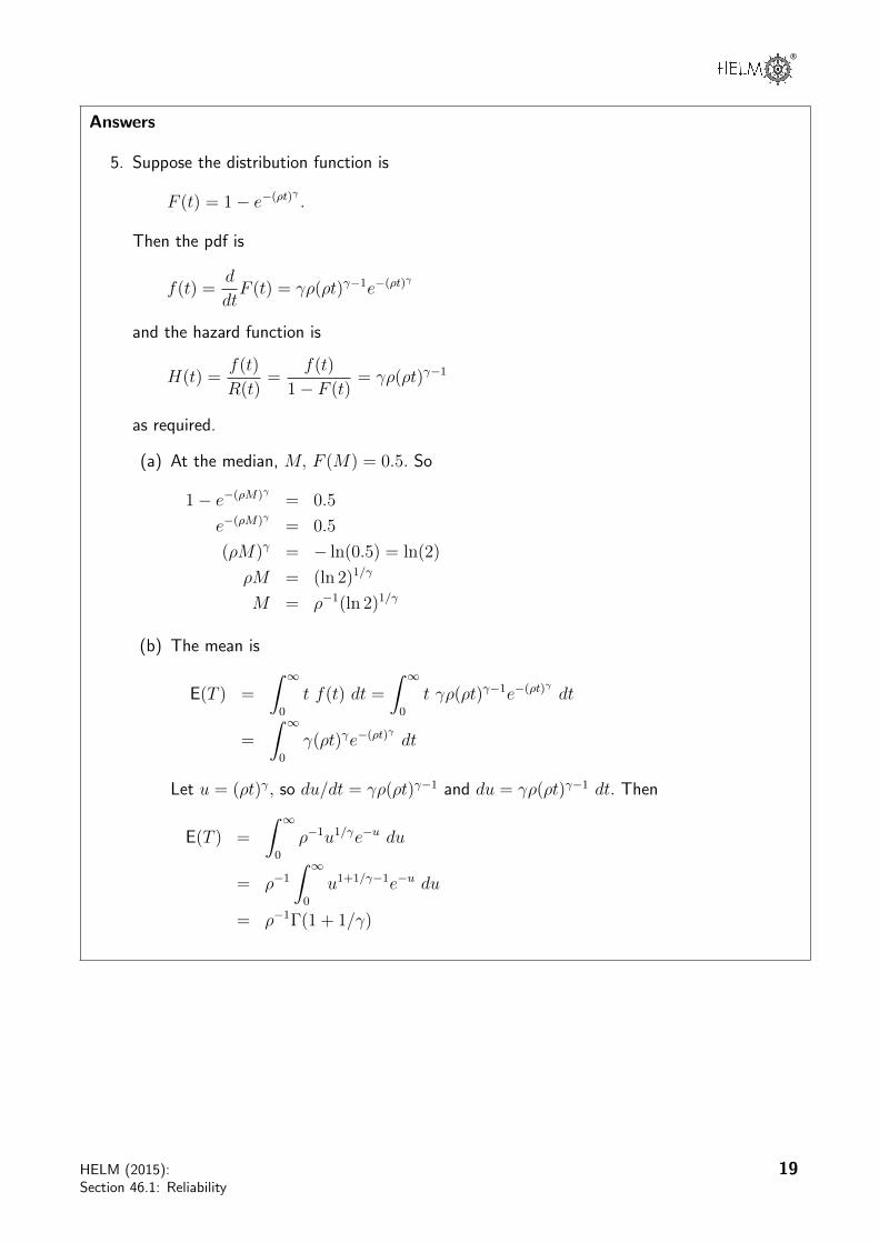
5. Suppose the distribution function is

F (t) = 1− e−(ρt)γ .

Then the pdf is

f(t) =d

dtF (t) = γρ(ρt)γ−1e−(ρt)γ

and the hazard function is

H(t) =f(t)

R(t)=

f(t)

1− F (t)= γρ(ρt)γ−1

as required.

(a) At the median, M, F (M) = 0.5. So

1− e−(ρM)γ = 0.5

e−(ρM)γ = 0.5

(ρM)γ = − ln(0.5) = ln(2)

ρM = (ln 2)1/γ

M = ρ−1(ln 2)1/γ

(b) The mean is

E(T ) =

∫ ∞0

t f(t) dt =

∫ ∞0

t γρ(ρt)γ−1e−(ρt)γ dt

=

∫ ∞0

γ(ρt)γe−(ρt)γ dt

Let u = (ρt)γ, so du/dt = γρ(ρt)γ−1 and du = γρ(ρt)γ−1 dt. Then

E(T ) =

∫ ∞0

ρ−1u1/γe−u du

= ρ−1

∫ ∞0

u1+1/γ−1e−u du

= ρ−1Γ(1 + 1/γ)


19

Answers

5. continued

(c) To find the variance we first find

E(T 2) =

∫ ∞0

t2 f(t) dt =

∫ ∞0

t2 γρ(ρt)γ−1e−(ρt)γ dt

=

∫ ∞0

γρ−1(ρt)γ+1e−(ρt)γ dt

Let u = (ρt)γ, so du/dt = γρ(ρt)γ−1 and du = γρ(ρt)γ−1 dt. Then

E(T 2) =

∫ ∞0

ρ−2u2/γe−u du

= ρ−2

∫ ∞0

u1+2/γ−1e−u du

= ρ−2Γ(1 + 2/γ)

So

V(T ) = E(T 2)− {E(T )}2

= ρ−2Γ(1 + 2/γ)− ρ−2{Γ(1 + 1/γ)}2

= ρ−2{Γ(1 + 2/γ)− {Γ(1 + 1/γ)}2}


®

Quality Control��

��46.2

IntroductionQuality control via the use of statistical methods is a very large area of study in its own right andis central to success in modern industry with its emphasis on reducing costs while at the sametime improving quality. In recent times, the Japanese have been extremely successful at applyingstatistical methods to industrial quality control and have gained a significant advantage over manyof their competitors. One need only think of the reputations enjoyed by Japanese motor, camera,TV, video, DVD and general electronics manufacturers to realize just how successful they havebecome. It is because of the global nature of modern industrial competition that quality control,or more precisely, statistical quality control has become an area of central importance to engineers.Manufacturing a product that the public wants to buy is no longer good enough. The productmust be of sufficiently high quality and sufficiently competitive price-wise that it is preferred to itscompetitors. Without statistical quality control methods it is extremely difficult, if not impossible,to either attain or maintain a truly competitive position.

#

"

!Prerequisites

Before starting this Section you should . . .

• be able to calculate means and standarddeviations from given data sets

• be able to estimate population means andstandard deviations from samples'

&

$

%

Learning OutcomesOn completion you should be able to . . .

• state what is meant by the term statisticalquality control.

• explain why different types of control chartsare necessary.

• construct and interpret a small variety ofcontrol charts, in particular those based onmeans and ranges.

• describe in outline the relationship betweenhypothesis testing and statistical qualitycontrol.

HELM (2015):Section 46.2: Quality Control

21

1. Quality controlBackgroundTechniques and methods for checking the quality of materials and the building of houses, temples,monuments and roads have been used over the centuries. For example, the ancient Egyptians hadto make and use precise measurements and adopt very high standards of work in order to build thePyramids. In the Middle Ages, the Guilds were established in Europe to ensure that new entrantsto the craft/trade maintained standards. The newcomer was required to serve a long period ofapprenticeship under the supervision of a master craftsman, and had to demonstrate his ability toproduce work of the appropriate quality and standard before becoming a recognized tradesman. Inmodern times the notion of quality has evolved through the stages outlined below.

Inspection

The Industrial Revolution introduced mass production techniques to the workplace. By the end of the19th century, production processes were becoming more complex and it was beyond the capabilitiesof a single individual to be responsible for all aspects of production. It is impossible to inspectquality into a product in the sense that a faulty product cannot be put right by means of inspectionalone. Statistical quality control can and does provide the environment within which the product ismanufactured correctly the first time. A process called acceptance sampling improves the averagequality of the items accepted by rejecting those items which are of unacceptable quality. In the1920s, mass production brought with it the production line and assembly line concepts. Henry Fordrevolutionised car production with the introduction of the mass production of the ‘Model T.’

Mass production resulted in greater output and lower prices, but the quality of manufactured outputbecame more variable and less reliable. There was a need to tackle the problem of the production ofgoods and parts of a fixed quality and standard. The solution was seen to be in the establishmentof inspection routines, under the supervision of a Quality Inspector. The first inspection proceduresrequired the testing of the entire production - a costly, time consuming and inefficient form of sortingout good and defective items.

Quality Control

The Second World War brought with it the need for defect-free products. Inspection departments nowcame to control the production process, and this resulted in the conformance to set specifications (thereduction of variability and the elimination of defects) being monitored and controlled throughoutproduction. Quality Control departments were separate from, and independent of, the manufacturingdepartments.

Quality Assurance

In turn, Quality Control evolved into Quality Assurance. The function of Quality Assurance is tofocus on assuring process and product quality through operational audits, the supplying of training,the carrying out of technical analysis, and the giving of advice on quality improvement. The roleof Quality Assurance is to consult with the departments (design and production for example) whereresponsibility for quality actually rests.

Total Quality Management

Quality Assurance has given way to Company Wide Quality Management or Total Quality Manage-ment. As the names imply, quality is no longer seen to be the responsibility of a single department,but has become the responsibility and concern of each individual within an organisation. A smallexecutive group sets the policy which results in targets for the various sections within the company.


®

For example, line management sets ‘do-able’ objectives; engineers to design attractive, reliable, andfunctional products; operators to produce defect-free products and staff in contact with customersto be prompt and attentive. Total Quality Management aims to measure, detect, reduce, eliminate,and prevent quality lapses, it should include not only products but also services, and address issueslike poor standards of service and late deliveries.

Statistical Quality Control

As a response to the impracticality of inspecting every production item, methods involving samplingtechniques were suggested. The behaviour of samples as an indicator of the behaviour of the entirepopulation has a strong statistical body of theory to support it.

A landmark in the development of statistical quality control came in 1924 as a result of the work ofDr. Walter Shewhart during his employment at Bell Telephone Laboratories. He recognised that ina manufacturing process there will always be variation in the resulting products. He also recognizedthat this variation can be understood, monitored, and controlled by statistical procedures. Shewhartdeveloped a simple graphical technique - the control chart - for determining if product variation iswithin acceptable limits. In this case the production process is said to be ‘in control’ and controlcharts can indicate when to leave things alone or when to adjust or change a production process.In the latter cases the production process is said to be ‘out of control.’ Control charts can be used(importantly) at different points within the production process.

Other leading pioneers in the field of quality control were Dr. H. Dodge and Dr. H. Romig. Shewhart,Dodge and Romig were responsible for much of the development of quality control based on samplingtechniques. These techniques formed what has become known as ‘acceptance sampling.’

Although the techniques of acceptance sampling and control charts were not widely adopted initiallyoutside Bell, during the 1920s many companies had established inspection departments as a meansof ensuring quality.

During the Second World War, the need for mass produced products came to the fore and in theUnited States in particular, statistical sampling and inspection methods became widespread. After theSecond World War, the Japanese in particular became very successful in the application of statisticaltechniques to quality control and in the United States, Dr. W.E. Deming and Dr. J.M. Duran spreadthe use of such techniques further into U.S. industry.

Statistical Process Control

The aim of statistical process control is to ensure that a given manufacturing process is as stable (incontrol) as possible and that the process operates around stated values for the product with as littlevariability as possible. In short, the aim is the reduction of variability to ensure that each product isof a high a quality as possible. Statistical process control is usually thought of as a toolbox whosecontents may be applied to solve production-related quality control problems. Essentially the toolboxcontains the major tools called:

• the Histogram; • scatter diagrams;• the Pareto chart; • check sheets;• cause-and-effect digrams; • control charts;• defect-concentration diagrams; • experimental design methods;• sampling inspection.

Note that some authors argue that experimental design methods should not be regarded as a statisticalprocess control tool since experimental design is an active process involving the deliberate change of


23

variables to determine their effect, while the other methods are based purely on the observation ofan existing process.

Control charts are a very powerful tool in the field of statistical process control. Before looking insome detail at control charts in general we will look at the relationship between specification limitsand tolerance limits since this can and does influence the number of defective items produced by amanufacturing process. It is this quantity that control charts seek to minimize.

Tolerance Limits and Specifications

An example of a specification for the manufacture of a short cylindrical spacer might be:

diameter: 1± 0.003 cm; length: 2± 0.001 cm.

Even though the ± differences here are the same (±0.003 in the case of the diameters and ±0.002in the case of the lengths), there is no reason why this should always be so. These limits are calledthe specification limits. During manufacture, some variation in dimensions will occur by chance.These variations can be measured by using the standard deviation of the distribution followed by thedimensions produced by the manufacturing process. Figure 1 below shows two normal distributionseach with so-called natural tolerance limits of 3σ either side of the mean.

Taking these limits implies that virtually all of the manufactured articles will fall within the naturaltolerance limits. Notice that in the top part of the figure the specification limits are rather widerthan the natural tolerance limits and that little if any wastage will be produced. One could arguethat in this case the manufacturing process is actually better than it needs to be and that this maycarry unnecessary costs. In the lower part of the figure the specification limits are narrower than thenatural tolerance limits and wastage will occur In general, a production process should aim to equatethe two types of limits to minimize both costs and wastage.

Control Charts

Any production process is subject to variability. Essentially, this variability falls into two categoriescalled chance causes and assignable causes. A production process exhibiting only chance causesis usually described as being ‘in control’ or ‘in statistical control’ whereas a production processexhibiting assignable causes is described as being ‘out of control.’ The basic aim of control chartsis the improvement of production processes via the detection of variability due to assignable causes.It is then up to people such as process operators or managers to find the underlying cause of thevariation and take action to correct the process. Figure 4 below illustrates the point.


®

Specification Limits

Idea

lV

alue

Tolerance Limits

Wastage

Production Line

ApplyCorrectiveAction

IdentifyBasicCause

VerifyActionandFollow-up

DetectAssignableProblem

Statistical Quality Control

Diagram 1 - Specification and Tolerance Limits

Diagram 2 - Correcting Assignable Variation

Idea

lV

alueWastage

3! 3!

3! 3!Tolerance Limits

Figure 4

A control chart basically consists of a display of ‘quality characteristics’ which are found from samplestaken from production at regular intervals. Typically the mean, together with a measure of thevariability (the range or the standard deviation) of measurements taken from the items being producedmay be the variables under consideration. The appearance of a typical control chart is shown belowin Figure 5.

The centre line on Figure 5 represents the ideal value of the characteristic being measured. Ideally,the points on the figure should hover around this value in a random manner indicating that onlychance variation is present in the production process. The upper and lower limits are chosen in sucha way that so long as the process is in statistical control, virtually all of the points plotted will fallbetween these two lines. Note that the points are joined up so that it is easier to detect any trendspresent in the data. At this stage, a note of caution is necessary. The fact that a particular control


25

chart shows all of its points lying between the upper and lower limits does not necessarily imply thatthe production process is in control. We will look at this aspect of control charts in some depth laterin this booklet. For now simply note that even points lying within the upper and lower limits thatdo not exhibit random behaviour can indicate that a process is either out of control or going out ofcontrol.

Sam

ple

Char

acte

rist

ic

Upper Limit

Ideal Value

Lower Limit

Sample Number

Figure 5: A typical control chart

It is also worth noting at this stage that there is a close connection between control charts andhypothesis testing. If we formulate the hypotheses:

H0 : the process is in control

H1 : the process is not in control

then a point lying with the upper and lower limits is telling us that we do not have the evidence toreject the null hypothesis and a point lying outside the upper and lower limits is telling us to rejectthe null hypothesis. From previous comments made you will realize that these statements are not anabsolute truth but that they are an indicative truth.

Control charts are very popular in industry. Before looking at particular types of control charts, thefollowing reasons are given for their popularity.

(a) They are simple to use. Production process operators do not need to be fluent in statisticalmethods to be able to use control charts.

(b) They are effective. Control charts help to keep a production process in control. Thisavoids wastage and hence unnecessary costs.

(c) They are diagnostic in the sense that as well as indicating when adjustments need to bemade to a process, they also indicate when adjustments do not need to be made.

(d) They are well-proven. Control charts have a long and successful history. They wereintroduced in the 1920s and have proved themselves over the years.


®

(e) They provide information about the stability of a production process over time. Thisinformation is of interest to production engineers for example. A very stable process mayenable fewer measurements to be taken - this has cost implications of course.

Control chart construction

In order to understand how control charts are constructed, consider the following scenario.

Part of a production line used by a manufacturer of instant coffee involves the use of a machine whichfills empty packets with coffee. The filler is set to fill each empty packet with 200 grams of coffee. Asthis is an electro-mechanical process, repeated over a long period of time, it is inevitable that therewill be some degree of variation in the amounts of coffee dispensed. The question that productionengineers will need to answer is “Is the variation sufficient to result in a significant ‘underfilling’, or‘overfilling’, of the packets?”

The following data (which represent the weights of a sample of 50 packets of 200 grams of coffee)are obtained from the production line:

200.0 197.8 200.1 200.6 198.7198.7 203.4 201.3 199.8 200.6202.2 196.4 199.2 199.9 200.3198.2 201.4 202.8 201.3 203.6201.9 199.7 198.5 199.8 202.4201.3 201.2 198.5 196.4 199.2202.4 202.4 197.9 201.3 200.8197.8 202.0 200.7 201.1 199.7201.3 197.6 200.9 201.6 196.2199.7 203.1 203.1 200.9 199.2

In this example, the data should be read from top left to bottom right, down the columns, that isfrom 200.0, 198.7, 202.2 and so on to 199.2.

Using Microsoft Excel, the data give the following numerical summaries:

x̄ = 200.298 ≈ 200.30 grams,

s = 1.842 ≈ 1.84 grams

Note that the summaries refer to a sample but, as the sample size is large (n = 50 ), these valuesmay be taken as estimates for the population parameters and we shall take their values as:

µ = 200.30 grams,

σ = 1.84 grams

A plot of the data from Excel is shown in Figure 5, known as an x̄̄x̄x-chart.


27

210

205

200

195

1 10 20 30 40 50

Wei

ght

(gm

)

Coffee packet number

Figure 6: Data plot chart

To the plotted series of data are added:

(a) a horizontal line representing the process mean of 200.30 grams

(b) two further horizontal lines representing the upper and lower control limits. The valuesof these limits are given by x̄± 3σ and are calculated as 205.8 and 194.8

These lines are called the Upper Control Limit (UCL) and the Lower Control Limit (LCL).

This process results in the x̄-chart Figure 7 below.

210

205

200

195

190

1 10 20 30 40 50

Wei

ght

(gm

)

Upper Control Limit

MeanValue

Lower Control Limit

Coffee packet number

Figure 7: Control chart with centre line and limits


®

In a production process, samples are taken at regular intervals, say every 10 mins., 15 mins., 30 mins,and so on, so that at least 25 samples (say) are taken. At this stage, we will be able to detect trends- looked at later in this workbook - in the data. This can be very important to production engineerswho are expected to take corrective action to prevent a production process going out of control. Thesize of the sample can vary, but in general n ≥ 4. Do not confuse the number of samples taken,with the sample size n.

The centre line, denoted by ¯̄x is given by the mean of the sample means

¯̄x =x̄1 + x̄2 + . . .+ x̄k

k

where k is the number of samples. ¯̄x is used as an estimator for the population mean µ.

Given that the sample size is n the upper and lower control limits are calculated as

UCL = ¯̄x+3s√n

LCL = ¯̄x− 3s√n

These limits are also known as action limits; if any sample mean falls outside these limits, actionhas to be taken. This may involve stopping the production line and checking and/or re-seting theproduction parameters.

In the initial example, a single sample of size n = 50 was used. In reality, with samples being takenat short time intervals, e.g. every 10 min., there is not sufficient time to weigh this many packages.Hence, it is common to use a much smaller sample size, e.g. n = 4 or 5.

Under these circumstances, it is not sensible (very small sample size may give inaccurate results) touse s as an estimate for σ the standard deviation of the population. In a real manufacturing process,the value of σ is almost always unknown and must be estimated.

Estimating the population standard deviation.

It is worth noting that there is, in practice, a distinction between the initial setting up of a control chartand its routine use after that. Initially, we need a sufficiently large sample to facilitate the accurateestimation of the population standard deviation σ. Three possible methods used to estimate are:

(a) Calculate the standard deviations of several samples, and use the mean of these values asan estimate for σ.

(b) Take a single, large size sample from the process when it is believed to be in control.Use the standard deviation s of this sample as an estimate for σ. Note that this was themethod adopted in the initial example.

(c) In industry, a widely used method for obtaining an unbiased estimate for σ uses thecalculation of the average range R̄ of the sample results. The estimate for σ is then givenby the formula:

σ̂ =R̄

d2

where d2 is a constant that depends on the sample size. For example, the Table given at the end ofthis Workbook, show that for n = 5, d2 = 2.326.

The control limits can now be expressed in the form:

¯̄x± 3R̄

d2√n


29

and, by a further simplification as:

¯̄x± A2R̄

A table for the constant A2 are given at the end of this Workbook (Table 1).

Example 5The following table shows the data obtained from 30 samples, each of size n = 4,taken from the ’instant coffee’ production line considered above. The table hasbeen extended to show the mean x̄ and the range R̄ of each sample. Find thegrand mean ¯̄x, the upper and lower control limits and plot the control chart. Youare advised that all of the necessary calculations have been done in Excel andthat you should replicate them for practice. You can, of course, use a dedicatedstatistics package such as MINITAB if you wish.

Sample Weight Weight Weight Weight Mean Range Sample Weight Weight Weight Weight Mean Range1 202.3 199.8 201.4 200.3 200.95 2.5 16 195.5 202.0 199.2 202.3 199.75 6.82 198.6 201.3 199.7 201.8 200.35 3.2 17 199.0 200.7 200.1 199.3 199.78 1.73 197.9 199.8 200.1 189.8 196.90 10.3 18 197.6 188.9 201.1 200.3 196.98 12.24 202.4 205.1 199.6 189.2 199.08 15.9 19 200.6 199.4 201.8 202.0 200.95 2.65 194.7 201.2 197.5 201.1 198.63 6.5 20 199.4 201.0 200.8 197.6 199.70 3.46 200.8 199.8 200.3 196.2 199.28 4.6 21 197.8 205.1 203.6 204.3 202.70 7.37 198.5 201.4 200.6 199.2 199.93 2.9 22 201.3 196.8 197.6 199.6 198.83 4.58 202.3 204.1 199.2 201.3 201.73 4.9 23 200.6 199.4 200.4 201.8 200.55 2.49 205.4 198.3 194.9 198.5 199.28 10.5 24 198.9 204.2 202.0 201.1 201.55 5.310 199.0 202.2 197.1 202.8 200.28 5.7 25 203.0 201.6 201.4 200.8 201.70 2.211 189.7 200.1 202.6 201.9 198.58 12.9 26 200.1 194.8 201.7 198.3 198.73 6.912 203.6 197.5 204.5 196.4 200.50 8.1 27 198.2 201.4 197.6 201.1 199.58 3.813 198.6 197.8 199.7 200.4 199.13 2.6 28 200.6 202.8 210.0 202.8 201.80 2.214 202.6 199.2 199.0 199.2 200.00 3.6 29 200.3 201.3 201.6 201.3 201.13 1.315 203.3 203.1 200.8 201.7 202.23 2.5 30 195.9 203.3 196.3 203.4 199.73 7.5

Solution

Using Excel, the following results are obtained:

¯̄x = 200.01 and R̄ = 5.56

Using these values, the control limits are defined as:

UCL = ¯̄x+ A2R̄ = 200.01 + 0.729× 5.56 = 204.06

and

LCL = ¯̄x− A2R̄ = 200.01− 0.729× 5.56 = 195.96


®

Solution (contd.)

UCL = 204.06

¯̄x = 200.1

LCL = 195.96

205.00

203.00

201.00

199.00

197.00

195.0010 20 30

Wei

ght

(gm

)

Sample number

Figure 8

Note that if the process is in control, the probability that a sample mean will fall outside the controllimits is very small. From the central limit theorem we know that the sample means follow (or at leastapproximately follow) a normal distribution and from tables it is easy to show that the probability ofa sample mean falling outside the region defined by the 3σ control limits is about 0.3%. Hence, if asample mean falls outside the control limits, there is an indication that there could be problems withthe production process. As noted before the process is then said to be out of control and processengineers will have to locate the cause of the unusual value of the sample mean.

Warning limits

In order to help in the monitoring of the process, it is common to find additional warning limitswhich are included on the control chart. The settings for these warning limits can vary but a commonpractice involves settings based upon two standard deviations. We may define warning limits as:

¯̄x± 2σ√n

Using the constant d2 defined earlier, these limits may be written as

¯̄x± 2R̄

d2√n


31

Example 6Using the data from Example 5, find the 2σ warning limits and revise the controlchart accordingly.

Solution

We know that ¯̄x = 200.01, R̄ = 5.56, and that the sample size n is 4. Hence:

¯̄x± 2R̄

d2√n

= 200.01± 2× 5.56

2.059×√

4= 200.01± 2.70

The warning limits clearly occur at 202.71 and 197.31. The control chart now appears as shownbelow. Note that the warning limits in this case have been shown as dotted lines.

UCL = 204.06

¯̄x = 200.1

LCL = 195.96

205.00

203.00

201.00

199.00

197.00

195.0010 20 30

Wei

ght

(gm

)

Sample number

Figure 9

Detecting trends

Control charts can also be used to detect trends in the production process. Even when all of thesample means fall within the control limits, the existence of a trend can show the presence of one,or more, assignable causes of variation which can then be identified and brought under control. Forexample, due to wear in a machine, the process mean may have shifted slightly.

Trends are detected by considering runs of points above, or below, the centre line. A run is definedas a sequence of consecutive points, all of which are on the same side of the centre line.

Using a plus (+) sign to indicate a point above, and a minus (−) sign to indicate a point below,the centre line, the 30 sample means used as the worked examples above would show the followingsequence of runs:

+ +−−−−−+−+−+−+ +−−−+−+−+ + + +−−+ +−


®

Considerable attention has been paid to the study of runs and theory has been developed. Simplerules and guidelines, based on the longest run in a chart have been formulated.

Listed below are eight tests that can be carried out on the chart. Each test detects a specific patternin the data plotted on the chart. Remember that a process can only be considered to be in control ifthe occurrence of points above and below the chart mean is random and within the control limits. Theoccurrence of a pattern indicates a special cause for the variation, one that needs to be investigated.

The eight tests

• One point more than 3 sigmas from the centre line.

• Two out of three points in a row more than two sigmas from the centre line (same side)

• Four out of five points in a row more than 1 sigma from centre line (same side)

• Eight points in a row on the same side of the centre line.

• Eight points in a row more than 1 sigma either side of the centre line.

• Six points in a row, all increasing or all decreasing.

• Fourteen points in a row, alternating up and down.

• Fifteen points in a row within 1 sigma of centre line (either side)

The first four of these tests are sometimes referred as the Western Electric Rules. They were firstpublished in the Western Electric Handbook issued to employees in 1956.

The RRR-Chart

The control chart based upon the sample means is only one of a number of charts used in qualitycontrol. In particular, to measure the variability in a production process, the chart is used. In thischart, the range of a sample is considered to be a random variable. The range has its own mean andstandard deviation. The average range R̄ provides an estimate of this mean, while an estimate ofthe standard deviation is given by the formula:

σ̂R = d3 ×R̄

d2

where d2 and d3 are constants that depend on sample size. The control limits for the R-chart aredefined as:

R̄± 3σ̂R = R̄± 3d3 ×R̄

d2

By the use of further constants, these control limits can be simplified to:

UCL = R̄×D4 and LCL = R̄×D3

Values for D3 and D4 are given in the table at the end of this workbook. For values of n ≤ 6 thevalue of D3 is zero.

Note that if the R-chart indicates that the process is not in control, then there is no point in tryingto interpret the x̄-chart.

Returning to the data we have used so far, the control limits for the chart will be given by:


33

UCL = R̄×D4 = 5.56× 2.282 ' 12.69

LCL = R̄×D3 = 0

since the sample size is only 4. Effectively, the LCL is represented by the horizontal axis in thefollowing chart.

10 20 300.00

2.00

4.00

6.00

8.00

10.00

12.00

14.00

16.00

UCL = 12.69

R̄ = 5.56

Sample Number

Sam

ple

Ran

ge(g

m)

Figure 10: Control Chart

Note that although the x̄-chart indicated that the process was in control, the R̄-chart shows thatin two samples, the ranges exceed the UCL. Hence, no attempt should be made to interpret thex̄-chart. Since the limits used in the x̄-chart are based upon the value of R̄, these limits will havelittle meaning unless the process variability is in control. It is often recommended that the R-chart beconstructed first and if this indicates that the process is in control then the x̄-chart be constructed.However you should note that in reality, both charts are used simultaneously.

Further control charts

The x̄-charts and the R-charts considered above are only two of the many charts which are used inquality control. If the sample is of size n > 10 then it may be better to use a chart based on thestandard deviation, the s-chart, for monitoring process variability. In practice, there is often little tochoose between the s-chart and the R-chart for samples of size n < 10 although it is worth notingthat the R-chart is easier to formulate thanks to the easier calculations.

Many control charts have a common appearance with a central line indicating a mean, a fixed setting,or perhaps a percentage of defective items, when the process is in control. In addition, the chartsinclude control limits that indicate the bounds within which the process is deemed to be in control.A notable exception to this is the CUSUM chart. This chart is not considered here, but see, forexample, Applied Statistics and Probability for Engineers, Montgomery and Runger, Wiley, 2002.


®

Pareto charts

A Pareto diagram or Pareto chart is a special type of graph which is a combination line graph andbar graph. It provides a visual method for identifying significant problems. These are arranged in abar graph by their relative importance. Associated with the work of Pareto is the work of JosephJuran who put forward the view that the solution of the ‘vital few’ problems are more important thansolving the ‘trivial many’ . This is often stated as the ‘80 20 rule’ ; i.e. 20% of the problems (thevital few) result in 80% of the failures to reach the set standards.

In general terms the Pareto chart is not a problem-solving tool, but it is a tool for analysis. Itsfunction is to determine which problems to solve, and in what order. It aims to identify and eliminatemajor problems, leading to cost savings.

Pareto charts are a type of bar chart in which the horizontal axis represents categories of interest,rather than a continuous scale. The categories are often types of defects. By ordering the bars fromlargest to smallest, a Pareto chart can help to determine which of the defects comprise the vital fewand which are the trivial many. A cumulative percentage line helps judge the added contribution ofeach category. Pareto charts can help to focus improvement efforts on areas where the largest gainscan be made.

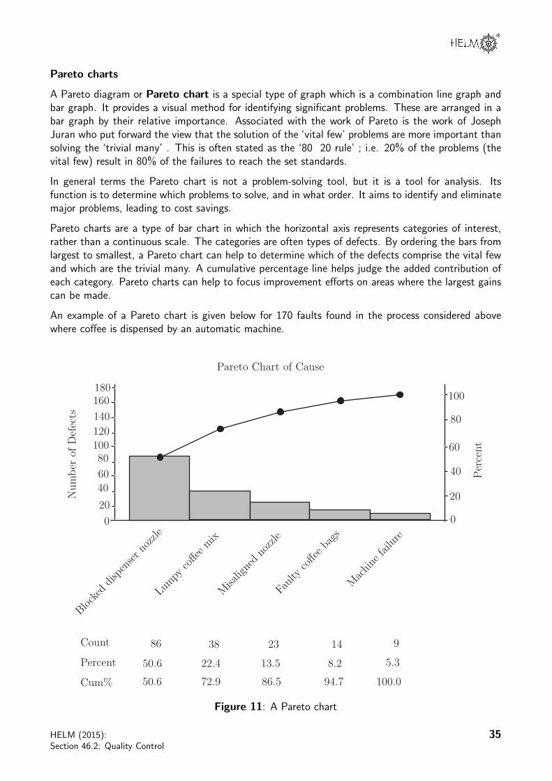
An example of a Pareto chart is given below for 170 faults found in the process considered abovewhere coffee is dispensed by an automatic machine.

Num

ber

ofD

efec

ts

Blocked

disp

enser no

zzle

Lumpy

co!e

emix

Misa

ligne

dno

zzle

Faulty

co!e

eba

gs

Machine

failu

re

Pareto Chart of Cause

0

20

4060

80100120

140

160

0

20

40

60

80

100180

Count 86 38 23 14 9

Percent 50.6 22.4 13.5 8.2 5.3

Cum% 50.6 72.9 86.5 94.7 100.0

Per

cent

Figure 11: A Pareto chart


35

TaskThe following table shows the data obtained from 30 samples, each of size n = 4,taken from a production line whose output is nominally 200 gram packets of tacks.Extend the table to show the mean x̄ and the range R̄ of each sample. Find thegrand mean ¯̄x, the upper and lower control limits and plot the x̄- and R̄-controlcharts. Discuss briefly whether you agree that the production process is in control.Give reasons for your answer. You are advised to do all of the calculations in Excelor use a suitable statistics package.

Sample Weight Weight Weight Weight Sample Weight Weight Weight Weight1 201.3 199.8 201.4 200.3 16 196.5 202.0 199.2 202.32 198.6 201.3 199.7 201.8 17 199.0 200.7 200.1 199.33 198.9 199.8 200.1 199.8 18 196.6 198.9 201.1 200.34 202.4 203.1 199.6 199.2 19 200.6 199.4 201.8 201.05 194.7 201.2 197.5 201.1 20 199.4 201.0 200.8 197.66 200.8 199.8 200.3 196.2 21 199.8 203.1 201.6 204.37 199.5 201.4 200.6 199.2 22 201.3 196.8 197.6 199.68 202.3 203.1 199.2 201.3 23 200.6 199.4 200.4 200.89 205.4 198.3 197.9 198.5 24 197.9 202.2 201.0 200.1

10 199.0 202.2 197.1 202.8 25 203.0 201.6 201.4 200.811 189.7 200.1 202.6 201.9 26 200.1 199.8 201.7 199.312 201.6 197.5 204.5 196.4 27 198.2 201.4 198.6 201.113 198.6 198.8 199.7 200.4 28 200.6 202.8 210.0 202.814 202.6 199.2 199.0 199.2 29 200.3 201.3 201.6 201.315 203.3 203.1 200.8 201.7 30 197.9 201.3 198.3 201.4

Your solution


®

Answer

The solution is given in two parts, first the x̄-control chart and secondly the R̄-control chart.

Part (i)

Using Excel, the following results are obtained: ¯̄x = 200.24 and R̄ = 3.88

Using these values, the control limits are defined as:

UCL = ¯̄x+ A2R̄ = 200.24 + 0.729× 3.88 = 203.07

and

LCL = ¯̄x− A2R̄ = 200.04− 0.729× 3.88 = 197.41

The x̄-chart is shown below.

10 20 30

205.00

203.00

201.00

199.00

197.00

195.00

UCL = 203.07

¯̄x = 200.24

LCL= 197.41

wei

ght

(gm

)

Sample number

Sam

ple

mea

n


37

Answer

Part (ii)

The control limits for the chart are given by:

UCL = R̄×D4 = 3.88× 2.282 = 8.85

LCL = R̄× F3 = 0

since the sample size is 4, so that the LCL is represented by the horizontal axis in the followingR-chart.

10 20 30Sample Number

Sam

ple

Ran

ge(g

m)

0.00

2.00

4.00

6.00

8.00

10.00

12.00

14.00

UCL = 8.85

R̄ = 3.88

Since one member of the R-chart exceeds the UCL we cannot say that the process is in control andconclude that the source of the error should be investigated and corrected.

Table 1: Some constants used in the construction of control limits

Sample d2 A2 D3 D4

Size (n)

2 1.128 1.880 0 3.2673 1.693 1.023 0 2.5744 2.059 0.729 0 2.2825 2.326 0.577 0 2.1146 2.543 0.483 0 2.0047 2.704 0.419 0.076 1.9248 2.847 0.373 0.136 1.8649 2.970 0.337 0.184 1.816

10 3.078 0.308 0.223 1.77715 3.472 0.223 0.347 1.65320 3.735 0.180 0.415 1.58525 3.931 0.153 0.459 1.541


Index for Workbook 46

Action limits 29

Conditional failure rate functionsee Hazard function

Control charts 24-38Control chart construction 27Control limit constants table 38

Eight tests 33Electronic component lifetime 6Estimating standard deviation 29Exponential distribution 4, 10

Gamma function 11

Hazard function 3,5,10

Instant coffee production 27, 30, 32

Lifetime distributions 3Light bulb lifetime 5Lower control limit (LCL) 28

Parallel design of components 7-9Pareto charts 35

Probability of failure 3Production line data 27, 30, 32, 35, 36Pumping engine bearing lifetime 12-13

Quality assurance 22Quality control 21-38

R-chart 33Reliability 2-20Reliability function 3Runs 32

Series design of components 7-9Standard deviation estimation 29Statistical process control 23Statistical quality control 23System reliability 7-9

Tolerance limits 24Total quality management 22Trend detection 32

Upper control limit (UCL) 28

Warning limits 31Weibull distribution 10

- cdf 10- mean 11- variance 11

x-chart 27, 32

Pattern detection tests 33

s-chart 34

EXERCISES14

about+the+helm+project+ -...

Documents